electron mean free path in a spherical shell geometry · electron mean free path in a spherical...

Electron Mean Free Path in a Spherical Shell Geometry

Alexander Moroz*WaVe-scattering.com

ReceiVed: February 2, 2008; ReVised Manuscript ReceiVed: March 25, 2008

Mean free path is calculated for the shell geometry under the assumptions of (i) diffusive, (ii) isotropic, and(iii) billiard, or Lambertian, scattering. Whereas in a homogeneous sphere case the difference between differentmodels of surface scattering is reflected merely by a different slope of the linear dependence of a mean freepath Leff on the sphere radius R, qualitatively different nonlinear dependencies on the inner and outer shellradii result for different model cases in the shell geometry. A linear behavior of Leff on the shell thickness (D)can only be established for the billiard model in the thin shell limit, in which case Leff ≈ 2D, whereas, in thesame limit, Leff ≈ (D/2)ln(2R/D) in the diffusive case and Leff ≈ 14(2RD)1/2/[3ln(2R/D)] in the isotropic case.The shell geometry turns out a very sensitive setup to distinguish between the different models of electronscattering, which could be performed in future experiments on single and well-controlled dielectric core-metal shell nanoparticles. This would enable one to more precisely assess the contribution of other mechanisms,such as chemical interface damping, to overall plasmon resonance damping. Preliminary experimental resultsare compatible with the billiard, or Lambertian, scattering model and appear to rule out both the Euler diffusivescattering and the isotropic scattering.

1. Introduction

Recently, a novel class of metallo-dielectric particles com-posed of a dielectric core and a metal shell, also callednanoshells, has gained a strong interest. These structures havethe unique property that their surface plasmon frequency isextremely sensitive to the thickness of the metal shell.1–5

Nanoshells offer significant advantages over conventionalimaging probes, including continuous and broad wavelengthtunability, far greater scattering and absorption coefficients,increased chemical stability, and improved biocompatibility.Becaus of their unique properties, the functionalized nanoshellshave been proposed as photothermal converters in a range ofapplications including photothermal cancer therapy and photo-thermally triggered drug release.6 Further applications involvethe use of gold nanoshell bioconjugates for molecular imagingin living cells,7 to improve single nanoparticle molecular sensorssensitivity8 and as molecular imaging multilabels.9

However, a practical realization of the applications that makesuse of the plasmon resonance, such as photothermal applica-tions,6 sensing,8 and multilabel applications,9 is strongly influ-enced by the line shape broadening.10 As well-known from thecase of homogeneous metallic particles,11–18 the line shape ofthe plasmon resonance in small metallic particles is significantlyaffected by its size. Assuming quasicontinuous energy bandsof electrons, that is, that the discrete quantum energy levelsbroadening exceeds the mean spacing between the levels, it isbelieved to be justified to apply a purely classical reasoningthat the line shape broadening effect is essentially geometric inits origin.11–14,17 The standard classical approach for describingthe size dependence of the dielectric function assumes that if aparticle size is comparable to or smaller than the mean free pathof conduction electrons in the bulk material (l∞),12,13,19 then thescattering of the conduction electrons from the particle surfaceresults in a reduced effective mean free path (Leff), and anincreased homogeneous line width—the full width at half-

maximum (fwhm)—of the dipole plasmon polariton (Γ), throughthe Mathiessen’s rule11–17

Γ)Γ0 +υF

Leff(1)

Here υF is the Fermi velocity of conduction electrons, and Γ0

) υF/l∞ describes the intrinsic bulk width of the dipole plasmonpolariton. The ratio υF/Leff may be classically interpreted as theeffective rate of scattering of the conduction electrons off theparticle surface. The line width Γ directly determines thedephasing time T2 ) 2p/Γ, where p is Planck’s constant, thequality factor (Q) of the resonance at an energy Eres via theformula Q ) Eres/Γ, and the local field enhancement factor |f|20

(in a harmonic model |f| ) Q).21

Surprisingly enough, and in striking contrast to the obviouspractical importance of the nanoshell case, there is no agreementregarding the relevant Leff in the spherical shell case. Contraryto a homogeneous sphere case (Appendix B), different ap-proximate formulas are abundant in the literature for Leff in thenanoshell case, often ad-hoc and not supported by any underly-ing model of surface scattering. In the case of thin shells, themost popular choice by far is to simply set Leff equal to theshell thickness (D).2–5,8 The usual reasoning is that, from theviewpoint of an electron, a thin shell is more comparable to athin film than to a solid nanosphere. Yet, it is not difficult toshow that the classical mean free path for a thin film diverges.Upon integrating the chord length L(θ) ) D/cos θ over θ ∈(0, π/2 - δ) (Figure 1)* E-mail: [email protected].

Figure 1. Definition of the parameters in a slab geometry. The chordlength is L(θ) ) D/cos θ, where D is the slab thickness.

J. Phys. Chem. C 2008, 112, 10641–10652 10641

10.1021/jp8010074 CCC: $40.75 2008 American Chemical SocietyPublished on Web 06/27/2008

D∫0

π⁄2-δ sin θ dθcos θ

)D∫δ

1 dxx

)Dln x|δ1

)D ln(1 ⁄ δ)f∞ (δf 0) (2)

To support the classical arguments leading to the mean freepath,

Lc )D (3)

one is thus forced to bail out by recalling seminal quantum-mechanical result for thin films. In the limit of pω , EF, withEF and ω being the Fermi energy and frequency, respectively,the result is22,23

LQM ≈ 23

D (4)

Another popular choice is the Granqvist and Hunderiresult.24,25 Let r1 and r2 be the radii of the inner and outersurfaces of the shell, respectively. Then, when eq 6 of ref 24 isrewritten in terms of the radii, the Granqvist and Hunderieffective mean free path reads

LGH ) [(r2 - r1)(r22 - r1

2)]1⁄3 )D[2(r2 ⁄ D)- 1]1⁄3 (5)

Equation 5 is sometime misquoted with a 1/2 prefactor,26,27 and,in order to fit better experimental results, is additionally scaledby yet another 1/2 factor.26,27 However, the Granqvist andHunderi result (eq 5) is rather a rough estimate of the meanfree path. To understand this expression, imagine a tangent tothe inner sphere; the length along the tangent between the twospheres is, upon applying the Pythagorean theorem, t ) �(r2

2

- r12). The formula is then equivalent to the cubic root of a

believed to be characteristic volume element Dt2, that is, LGH

) (Dt2)1/3.Xu28 took into account that there are electron trajectories

within a shell that (i) connect the inner and the outer surface ofthe shell and that (ii) connect two points on the outer surfacewithout cutting the inner shell surface. Let θ be the anglebetween the electron trajectory and the radius at the cross pointon the outer shell surface (Figure 2). Then, the first set oftrajectories occurs when sin θ e r1/r2, whereas the second setof trajectories takes place when sin θ > r1/r2. The separationpoint between the two different sets of trajectories is given by

sin θc ) r1 ⁄ r2 (6)

The corresponding lengths of the two set of trajectories as afunction of θ are then

L(θ)) {r2cos θ- √r12 - r2

2 sin2 θ, θe θc

2r2 cos θ, θ > θc

(7)

The resulting mean free path is then given by

LXu )∫0

π⁄2L(θ) sin θ dθ (8)

However, the expression is largely incomplete, because thecontribution of the points on the inner shell boundary to themean free path has been entirely neglected.

Kachan and Ponyavina 31,32 suggested the following formulafor the electron mean free path in a shell geometry:

LKP )R[ 1

1+ q2- q

2- 1

4(1- q2)

(1+ q2)(1- q) ln

(1- q)(1+ q)] (9)

where R ) r2 and q ) r1/r2. The formula has been employedby, for example, Boris and Nikolai Khlebtsov10 and others.21

However, the Kachan and Ponyavina result for mean free pathis again unsatisfactory, because it does not correspond to anycustomary model assumptions about the surface scattering.

Eventually, in a seemingly unrelated field of billiards, aremarkably simple formula has been derived, which yields themean free path entirely in terms of the geometrical parametersof a bounded and connected domain Q under consideration29,30

LB )|Q| · |Sd-1|

|∂Q| · |Bd-1|(10)

Here, |Q| is the volume of Q, |∂Q| is the area of the surface ∂Qof Q, |Sd-1| is the surface of a unit sphere in Rd, and |Bd-1| )|Sd-2|/(d - 1) is the volume of a unit ball in Rd-1. One has thefollowing relations

S1 ) 2π, S2 ) 4π, B1 ) 2, B2 )π (11)

In particular, for planar billiards (d ) 2)

LB )π|Q||∂Q|

(12)

whereas for three-dimensional billiards (d ) 3)

LB )4|Q||∂Q|

(13)

Thus, in the present case of a spherical shell geometry,

LB )4(r2

3 - r13)

3(r22 + r1

2)) 4R

31- q3

1+ q2(14)

In the following, the mean free path for shell geometry willbe calculated (i) on assuming Euler diffusive surface scattering11

and (ii) under the assumption of a homogeneous and isotropicelectron distribution within a shell. Further, the billiard formula(eq 14) in the nanoshell case will be confirmed by an explicitaveraging procedure. It will be demonstrated that the very sameresult also follows upon assuming that the electron scatteringevents on the domain surface ∂Q conspire to produce a“Lambertian” surface (see Section 2.1). It will be shown thatpreliminary experimental results,3–5,8,36 which were performedexclusively within the range D/R j 0.25, are compatible withthe billiard, or Lambertian, scattering model and rule out boththe Euler diffusive scattering and the isotropic scattering. Thesuccess of the Euler diffusive scattering in the homogeneoussphere case11–14 seems to be purely accidental, since all thescattering models yield a linear dependence of the mean freepath on the sphere radius with minor differences in the slope(see Appendix B). Contrary to the homogeneous sphere case,

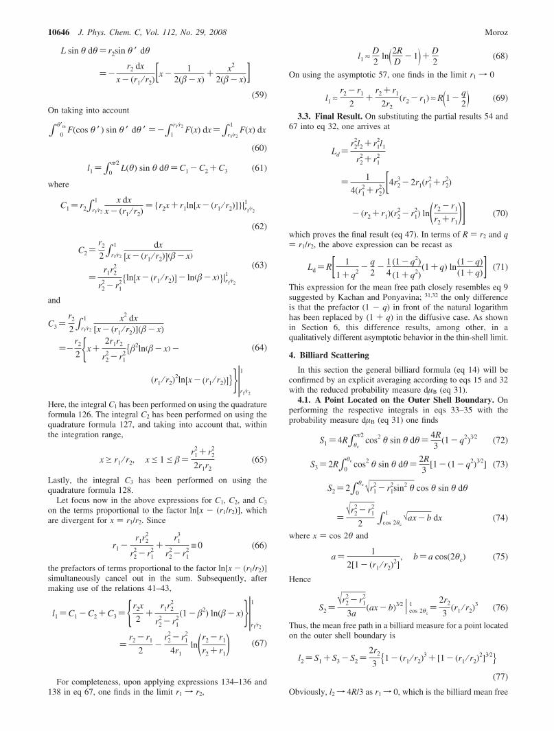
Figure 2. Spherical shell geometry and the definition of parametersfor a point on the outer shell boundary. The chord length L(θ) is givenby eq 7. Typical triangles used to calculate L(θ) are shown by dashedlines.

10642 J. Phys. Chem. C, Vol. 112, No. 29, 2008 Moroz

the mean free path in the shell geometry turns out to be muchmore sensitive to underlying model assumptions of electronsurface scattering. Consequently, future experiments on singleand well-controlled dielectric core-metal shell nanoparticles canmuch easier differentiate between competing models of surfacescattering. The outline of the article is as follows. In Section 2we review different models of surface scattering, summarizenotation, and give some basic definitions. Section 3 deals withthe mean free path for a diffusive scattering. The resulting meanfree path is given by eq 47, or, in terms of R and q, by eq 71.As a byproduct, an explicit expression for LXu is obtained byperforming the integral in eq 8 (see eqs 54 and 55). The billiardformula (eq 14) in the spherical shell case is confirmed inSection 4. The mean free path for an isotropic scattering isdetermined by eq 85 and is derived in Section 5. Section 6summarizes asymptotic behavior for different models, both inthe thin shell and in the vanishing core limits. In Section 7, themain properties of the billiard model are singled out. Compari-son with experimental data is reviewed in Section 7.1. Theoreti-cal and practical implications are summarized in Section 7.2.We then conclude by Section 8. Intermediary calculational stepstogether with the wording of the Birkhoff-Khinchin theoremand a derivation of the billiard formula in its general form (eq10) are supplied as Supporting Information.

2. Notation and Definitions

At any point P of the boundary surface ∂Q of Q let us introducethe spherical coordinates with the origin at P and with the z-axisalong the inward normal. Let L(θ, �) be the length of the straightline PP′ connecting the point P with an opposite boundary pointP′ at an angles (θ, �) to the inward normal at P. The averagingover different chord lengths L(θ, �) emanating from P will involvean integration over the solid angle of 2π-steradians above thetangent plane at the point P, that is, with the integration range θ ∈(0, π/2), � ∈ (0, 2π), with a measure dµ(θ, �),

lP )∫ L(θ, �) dµ(θ, �) (15)

The resulting mean free path is then defined by

Leff )∫

∂QlP dS

|∂Q|(16)

2.1. Surface Scattering Models. Euler Model. Out of thevarious surface scattering models the Euler diffusive surfacescattering model11 is the oldest one. The model is concernedwith the trajectories immediately after individual scattering

events. The electron reflection on the boundary surface is takento be fully isotropic, meaning there is equal probability forelectrons to be scattered at any angle with respect to the surfacenormal. For that reason, the model is sometime referred to asthe isotropic scattering model.14–16 The resulting probabilitymeasure in the spherical coordinates with the origin at a givensurface point is then

dµd ) cdsin θ dθ d� (17)

where the normalization factor

cd-1 )∫0

π⁄2sin θ dθ ∫0

2πd�) 2π (18)

Isotropic Model. In contrast to the Euler model,11 an isotropicscattering is concerned with the trajectories immediately beforescattering events. No explicit assumption is made aboutindividual scattering events at the enclosure boundary exceptthat the scattering events conspire to maintain a homogeneousand isotropic particle distribution in the enclosure Q.13 To findthe corresponding measure for the chord lengths, the followinggedanken experiment is performed. Assume that the enclosureboundary has been switch on instantaneously from its imperme-able state to a fully permeable state. Let us now consider theamount of particles that will be detected by a detector locatedat a given enclosure boundary point P at a particular angle withrespect to the inward normal to the enclosure boundary.Obviously, the number of detected particles will be proportionalto L(θ, �). Each particle arriving at an angle (θ, �) to thedetector then transversed the length L(θ, �) from the latestcollision at the boundary surface. This results in the followingmeasure in the spherical coordinates,

dµi ) ciL(θ, �) sin θ dθ d� (19)

with the normalization factor

ci-1 )∫0

π⁄2sin θ dθ ∫0

2πL(θ, �) d� (20)

Billiard Scattering Model. The billiard scattering modelpresumes a specular reflection at the enclosure boundary, thatis, the angle of incidence equals the angle of reflection. Thisallows one to unambiguously follow any given electron trajec-tory. In contrast to previous models, further considerations inthe billiard case follow in the phase space. The latter is M ) Qj× Sd-1, where Qj is the closure of the domain Q, and Sd-1 is the(d - 1)-dimensional unit sphere of all velocity vectors. Whatis eventually of the main importance is actually the “boundary”subspace M of the phase space M, defined as

M : ) {x) (s, v) ∈ M : s ∈ ∂Q, v · n(s)g 0} (21)

Obviously, the configuration subspace of M is the boundary ∂Qof Q and velocity vectors V ∈ M are all possible outgoing unitvelocity vectors (note that the scalar product v ·n of v with theinward normal n at s ∈ ∂Q is required to be positive) resultingfrom reflections at ∂Q. In brief, the subset M consists of all thepoints of the phase space M immediately after reflections at∂Q.

Select a set of electrons immediately after their reflections at∂Q. By the above definition, such a set forms a subset, call itA, of M. The electrons of the initial set A will continue theiruniform straightforward motion, or a flow, until they reflect at∂Q again, in which case the set A ⊂ M will transform into a setTA ⊂ M, etc. These repeating transformations of the initial setA define a map, T : Af TA, which is usually called the billiardmap. After subsequent reflections at ∂Q, the initial set A is thusmapped into sets TA, T2A, etc, and undergoes continuous

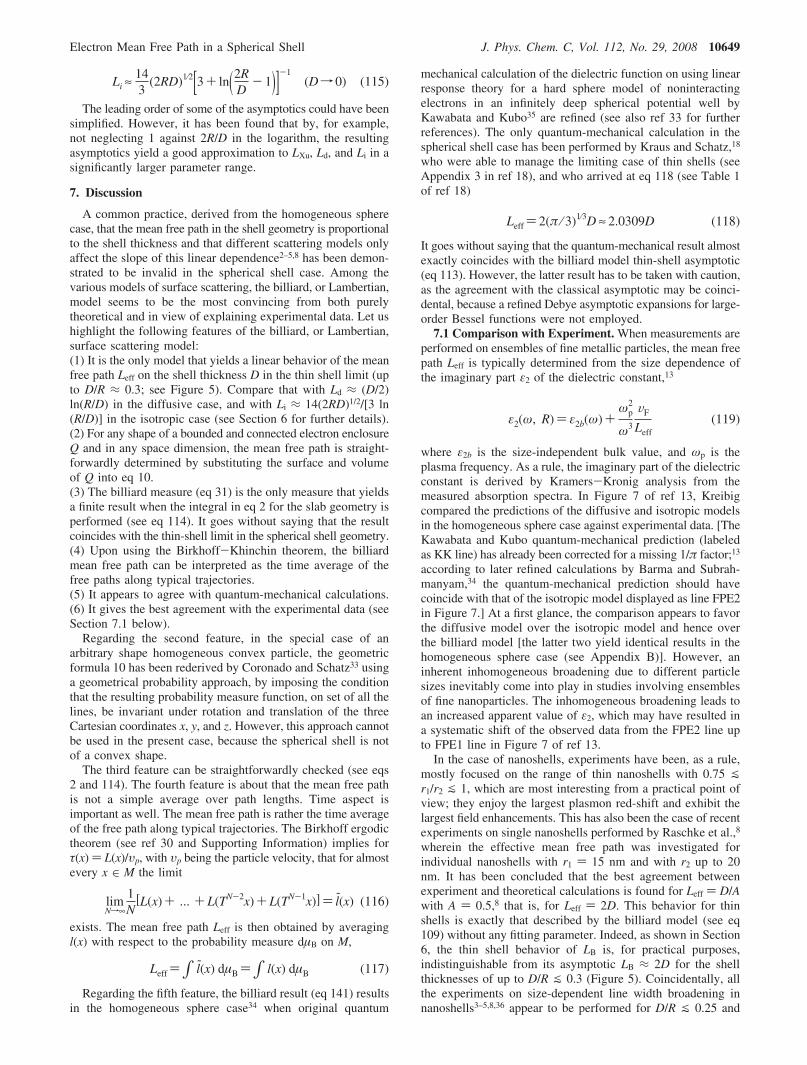
Figure 3. The mean free path in the spherical shell case for differentsurface scattering models as a function of the ratio D/R, where D isthe shell thickness and R is the shell outer radius.

Electron Mean Free Path in a Spherical Shell J. Phys. Chem. C, Vol. 112, No. 29, 2008 10643

changes in its underlying configuration and velocity subsets,which will spread or shrink depending on the geometry of ∂Q.Obviously, when focusing on either the configuration or velocitysubset of A, the corresponding Lebesgue measure of such asubset will change after each collision. The billiard measure isthe measure that is invariant under subsequent reflections ofthe initial set A ⊂ M of electrons and yields the very samemeasure of the initial set A after any reflection. In other words,

µB(A)) µB(TA)) µB(T2A)) ... ) µB(TnA) (22)

The resulting invariant measure in the spherical coordinatesis29,30

dµB ) cB(v · n) sin θ dθ d�) cBcos θ sin θ dθ d� (23)

with the normalization factor

cB-1 )∫0

π⁄2cos θ sin θ dθ∫0

2πd�) |B2|)π (24)

Note the extra “cos θ” factor in the billiard measure17 withregard to the Euler measure.17 The “cos θ” factor is tocompensate against the Jacobian of the transformation T :AfTA. Indeed, one finds

|det DT(x)|) cos θcos θ1

(25)

where the θ and θ1 are the angles of the unit velocity vectorsof the phase space points x and Tx, respectively, with regard tothe inward normal at the projections of x and Tx onto ∂Q (seepp 110-112, 116-118, and Figure IV.2 of ref 30). Hence, whenthe measure of TA is calculated by the substitution of variableswith regard to the map T : A f TA,

µB(TA)) 2∫TAcos θ1 ds1 dv1 ) 2∫A

cos θ1|det DT(x)| ds dv

) 2∫Acos θ1

cos θcos θ1

ds dv) µB(A)

(26)

where dv ) sin θ dθ d� is the Lebesgue measure on Sd-1 ford ) 3, and ds is the Lebesgue measure on ∂Q. Physically, theextra “cos θ” factor in the billiard measure17 with regard to theEuler measure17 can be interpreted as that the electron enclosuresurface is a “Lambertian” surface. The latter is distinguishedby a fact that the radiant intensity observed from it is directlyproportional to the cosine of the angle θ between the observer’sline of sight and the surface normal; hence, when an areaelement on the surface is viewed from any angle, it has the

same radiance. (An example a perfect Lambertian radiator is ablackbody, and, to a large extent, the Sun in the visiblespectrum.) Consequently, the billiard measure17 can be inter-preted as that the electron scattering events on the domainsurface ∂Q conspire to produce a diffusive “Lambertian” surface.The condition of specular reflections can then be abandoned.

2.2. Shell Geometry—Summary of Basic Formulas. Shellgeometry brings about several simplifications to the abovegeneral considerations. First, in virtue of the axial symmetryalong the inward normal, the chord length L(θ, �) emanatingfrom any fixed P does not depend on �, and the integration ineq 15 over � is trivial. Therefore, one can replace eq 15 by

lP )∫ L(θ) dµ(θ) (27)

with the following reduced probability measures

dµd(θ)) sin θ dθ (28)

dµi(θ)) ciL(θ) sin θ dθ (29)

with the normalization factor ci being the inverse of lP in thediffusive case, wherein the normalization factor ci is

ci-1 )∫0

π⁄2L(θ) sin θ dθ) lP;d (30)

and

dµB(θ)) 2cos θ sin θ dθ (31)

Second, because of the spherical symmetry, for all the pointson the shell-ambient interface the very same average chordlength lP ) l2 is obtained after performing the integral in eq27. Similarly, all the points on the shell-core interface areequivalent when the value of the integral in eq 27 is concerned;in this case the average chord length is denoted by l1.Consequently, the surface integral in eq 16 is replaced by asimple algebraic relation. The formula for the resulting meanfree path then simplifies from eq 16 to

Leff )r2

2l2 + r12l1

r22 + r1

2(32)

For a point on the outer shell boundary (Figure 2), that is,on the shell-ambient interface, the chord length L(θ) is givenby eq 7. Upon substituting eq 7 into the integral in eq 27, threedifferent integrals result,

S1 ) 2R∫θc

πcos θ dµ(θ) (33)

S2 )∫0

θc √r12 - r2

2sin2 θ dµ(θ) (34)

S3 )R∫0

θc cos θ dµ(θ) (35)

where, as usual, R ) r2 and the limit point θc in the aboveintegrals is defined by eq 6.

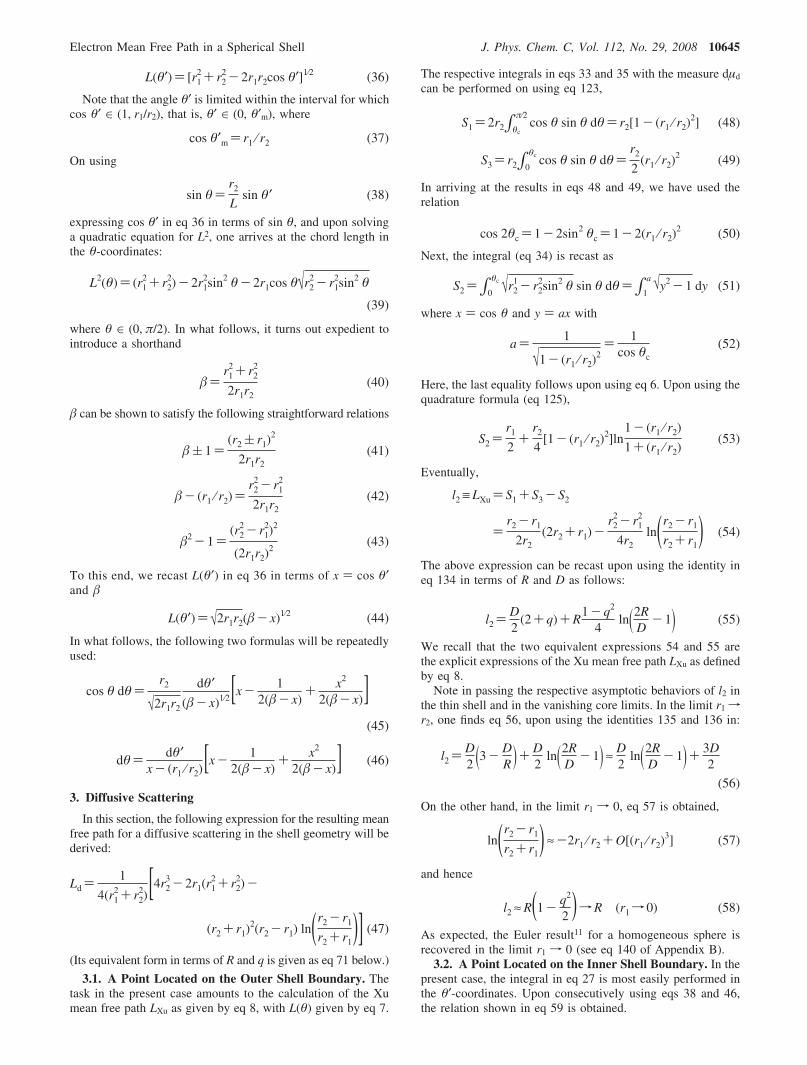
For points on the inner shell boundary, or, on the shell-coreinterface, it turns out that the integral in eq 27 with the diffusiveand billiard measures can be more easily performed in thespherical coordinates with the origin coinciding with the centersof the two concentric spheres forming the shell boundaries andwith the z-axis oriented along the segment connecting the originwith the point P. In what follows, the spherical coordinates atthe point P will be referred to as the θ-coordinates, and thelatter coordinates as the θ′-coordinates. (See Figure 4 for θ andθ′ definitions.) The chord length can be most easily found inthe θ′-coordinates. Indeed, on applying the law of cosines (eq122),

Figure 4. Spherical shell geometry and the definition of parametersfor a point on the inner shell boundary. The chord length L inθ-coordinates is given by eq 36, and that in θ′-coordinates is given byeq 39. A triangle used to calculate the highlighted chord length L bythe cosine formula (eq 122) in θ′-coordinates is shown by dashed lines.


L(θ′)) [r12 + r2

2 - 2r1r2cos θ′]1⁄2 (36)

Note that the angle θ′ is limited within the interval for whichcos θ′ ∈ (1, r1/r2), that is, θ′ ∈ (0, θ′m), where

cos θ′m ) r1 ⁄ r2 (37)

On using

sin θ)r2

Lsin θ′ (38)

expressing cos θ′ in eq 36 in terms of sin θ, and upon solvinga quadratic equation for L2, one arrives at the chord length inthe θ-coordinates:

L2(θ)) (r12 + r2

2)- 2r12sin2 θ- 2r1cos θ√r2

2 - r12sin2 θ

(39)

where θ ∈ (0, π/2). In what follows, it turns out expedient tointroduce a shorthand

�)r1

2 + r22

2r1r2(40)

� can be shown to satisfy the following straightforward relations

�( 1)(r2 ( r1)

2

2r1r2(41)

�- (r1 ⁄ r2))r2

2 - r12

2r1r2(42)

�2 - 1)(r2

2 - r12)2

(2r1r2)2

(43)

To this end, we recast L(θ′) in eq 36 in terms of x ) cos θ′and �

L(θ′)) √2r1r2(�- x)1⁄2 (44)

In what follows, the following two formulas will be repeatedlyused:

cos θ dθ)r2

√2r1r2

dθ′(�- x)1⁄2[x- 1

2(�- x)+ x2

2(�- x)](45)

dθ) dθ′x- (r1 ⁄ r2)

[x- 12(�- x)

+ x2

2(�- x)] (46)

3. Diffusive Scattering

In this section, the following expression for the resulting meanfree path for a diffusive scattering in the shell geometry will bederived:

Ld )1

4(r12 + r2

2)[4r23 - 2r1(r1

2 + r22)-

(r2 + r1)2(r2 - r1) ln(r2 - r1

r2 + r1)] (47)

(Its equivalent form in terms of R and q is given as eq 71 below.)

3.1. A Point Located on the Outer Shell Boundary. Thetask in the present case amounts to the calculation of the Xumean free path LXu as given by eq 8, with L(θ) given by eq 7.

The respective integrals in eqs 33 and 35 with the measure dµd

can be performed on using eq 123,

S1 ) 2r2∫θc

π⁄2cos θ sin θ dθ) r2[1- (r1 ⁄ r2)

2] (48)

S3 ) r2∫0

θc cos θ sin θ dθ)r2

2(r1 ⁄ r2)

2 (49)

In arriving at the results in eqs 48 and 49, we have used therelation

cos 2θc ) 1- 2sin2 θc ) 1- 2(r1 ⁄ r2)2 (50)

Next, the integral (eq 34) is recast as

S2 )∫0

θc √r21 - r2

2sin2 θ sin θ dθ)∫1

a √y2 - 1 dy (51)

where x ) cos θ and y ) ax with

a) 1

√1- (r1 ⁄ r2)2) 1

cos θc(52)

Here, the last equality follows upon using eq 6. Upon using thequadrature formula (eq 125),

S2 )r1

2+

r2

4[1- (r1 ⁄ r2)

2]ln1- (r1 ⁄ r2)

1+ (r1 ⁄ r2)(53)

Eventually,

l2 ≡ LXu ) S1 + S3 - S2

)r2 - r1

2r2(2r2 + r1)-

r22 - r1

2

4r2ln(r2 - r1

r2 + r1) (54)

The above expression can be recast upon using the identity ineq 134 in terms of R and D as follows:

l2 )D2

(2+ q)+R1- q2

4ln(2R

D- 1) (55)

We recall that the two equivalent expressions 54 and 55 arethe explicit expressions of the Xu mean free path LXu as definedby eq 8.

Note in passing the respective asymptotic behaviors of l2 inthe thin shell and in the vanishing core limits. In the limit r1fr2, one finds eq 56, upon using the identities 135 and 136 in:

l2 )D2 (3- D

R )+ D2

ln(2RD

- 1) ≈ D2

ln(2RD

- 1)+ 3D2

(56)

On the other hand, in the limit r1 f 0, eq 57 is obtained,

ln(r2 - r1

r2 + r1) ≈-2r1 ⁄ r2 +O[(r1 ⁄ r2)

3] (57)

and hence

l2 ≈ R(1- q2

2 )fR (r1f 0) (58)

As expected, the Euler result11 for a homogeneous sphere isrecovered in the limit r1 f 0 (see eq 140 of Appendix B).

3.2. A Point Located on the Inner Shell Boundary. In thepresent case, the integral in eq 27 is most easily performed inthe θ′-coordinates. Upon consecutively using eqs 38 and 46,the relation shown in eq 59 is obtained.


L sin θ dθ) r2sin θ ′ dθ

)-r2 dx

x- (r1 ⁄ r2)[x- 1

2(�- x)+ x2

2(�- x)](59)

On taking into account

∫ 0

θ′m F(cos θ ′ ) sin θ ′ dθ ′ )-∫1

r1⁄r2 F(x) dx)∫r1⁄r2

1F(x) dx

(60)

l1 )∫0

π⁄2L(θ) sin θ dθ)C1 -C2 +C3 (61)

where

C1 ) r2∫r1⁄r2

1 x dxx- (r1 ⁄ r2)

) {r2x+ r1ln[x- (r1 ⁄ r2)]}|r1⁄r2

1

(62)

C2 )r2

2∫r1⁄r2

1 dx[x- (r1 ⁄ r2)](�- x)

)r1r2

2

r22 - r1

2{ln[x- (r1 ⁄ r2)]- ln(�- x)}|r1⁄r2

1(63)

and

C3 )r2

2∫r1⁄r2

1 x2 dx[x- (r1 ⁄ r2)](�- x)

)-r2

2 {x+2r1r2

r22 - r1

2{�2ln(�- x)-

(r1 ⁄ r2)2ln[x- (r1 ⁄ r2)]}}|r1⁄r2

1

(64)

Here, the integral C1 has been performed on using the quadratureformula 126. The integral C2 has been performed on using thequadrature formula 127, and taking into account that, withinthe integration range,

xg r1 ⁄ r2, xe 1e �)r1

2 + r22

2r1r2(65)

Lastly, the integral C3 has been performed on using thequadrature formula 128.

Let focus now in the above expressions for C1, C2, and C3

on the terms proportional to the factor ln[x - (r1/r2)], whichare divergent for x ) r1/r2. Since

r1 -r1r2

2

r22 - r1

2+

r13

r22 - r1

2≡ 0 (66)

the prefactors of terms proportional to the factor ln[x - (r1/r2)]simultaneously cancel out in the sum. Subsequently, aftermaking use of the relations 41–43,

l1 )C1 -C2 +C3 ) {r2x

2+

r1r22

r22 - r1

2(1- �2) ln(�- x)}|r1⁄r2

1

)r2 - r1

2-

r22 - r1

2

4r1ln(r2 - r1

r2 + r1) (67)

For completeness, upon applying expressions 134–136 and138 in eq 67, one finds in the limit r1 f r2,

l1 ≈ D2

ln(2RD

- 1)+ D2

(68)

On using the asymptotic 57, one finds in the limit r1 f 0

l1 ≈r2 - r1

2+

r2 + r1

2r2(r2 - r1) ≈ R(1- q

2) (69)

3.3. Final Result. On substituting the partial results 54 and67 into eq 32, one arrives at

Ld )r2

2l2 + r12l1

r22 + r1

2

) 1

4(r12 + r2

2)[4r23 - 2r1(r1

2 + r22)

- (r2 + r1)(r22 - r1

2) ln(r2 - r1

r2 + r1)] (70)

which proves the final result (eq 47). In terms of R ) r2 and q) r1/r2, the above expression can be recast as

Ld )R[ 1

1+ q2- q

2- 1

4(1- q2)

(1+ q2)(1+ q) ln

(1- q)(1+ q)] (71)

This expression for the mean free path closely resembles eq 9suggested by Kachan and Ponyavina; 31,32 the only differenceis that the prefactor (1 - q) in front of the natural logarithmhas been replaced by (1 + q) in the diffusive case. As shownin Section 6, this difference results, among other, in aqualitatively different asymptotic behavior in the thin-shell limit.

4. Billiard Scattering

In this section the general billiard formula (eq 14) will beconfirmed by an explicit averaging according to eqs 15 and 32with the reduced probability measure dµB (eq 31).

4.1. A Point Located on the Outer Shell Boundary. Onperforming the respective integrals in eqs 33–35 with theprobability measure dµB (eq 31) one finds

S1 ) 4R∫θc

π⁄2cos2 θ sin θ dθ) 4R

3(1- q2)3⁄2 (72)

S3 ) 2R∫0

θc cos2 θ sin θ dθ) 2R3

[1- (1- q2)3⁄2] (73)

S2 ) 2∫0

θc √r12 - r1

2sin2 θ cos θ sin θ dθ

)√r2

2 - r12

2 ∫cos 2θc

1 √ax- b dx (74)

where x ) cos 2θ and

a) 1

2[1- (r1 ⁄ r2)2]

, b) a cos(2θc) (75)

Hence

S2 )√r2

2 - r12

3a(ax- b)3⁄2 | cos 2θc

1 )2r2

3(r1 ⁄ r2)

3 (76)

Thus, the mean free path in a billiard measure for a point locatedon the outer shell boundary is

l2 ) S1 + S3 - S2 )2r2

3 {1- (r1 ⁄ r2)3 + [1- (r1 ⁄ r2)

2]3⁄2}(77)

Obviously, l2f 4R/3 as r1f 0, which is the billiard mean free


path for a homogeneous sphere (see eq 141 of Appendix B).4.2. A Point Located on the Inner Shell Boundary. Upon

consecutively using eqs 38 and 45,

2L cos θ sin θ dθ) 2r2cos θ sin θ′ dθ

) -2r2

2

√2r1r2

dx

(�- x)1⁄2[x- 12(�- x)

+ x2

2(�- x)] (78)

On taking into account eq 60,

l1 ) 2∫0

π⁄2L(θ) cos θ sin θ dθ)C1 -C2 +C3 (79)

where

C1 )2r2

2

√2r1r2

∫r1⁄r2

1 x dx

(�- x)1⁄2

) -4r2

2

3√2r1r2

(2�+ x)(�- x)1⁄2 | r1⁄r2

1

(80)

C2 )r2

2

√2r1r2

∫r1⁄r2

1 dx

(�- x)3⁄2)

2r22

√2r1r2

1

(�- x)1⁄2 |r1⁄r2

1 (81)

and

C3 )r2

2

√2r1r2

∫r1⁄r2

1 x2dx

(�- x)3⁄2

)2r2

2

√2r1r2

-13

(�- x)3⁄2 + 2�(�- x)1⁄2 + �2

(�- x)1⁄2 |r1⁄r2

1

(82)

Here, the integral C1 has been performed on using the quadratureformula 129. The integral C2 has been performed upon usingthe quadrature formula 130, and taking into account that theinequalities of eq 65 hold within the integration range. Lastly,the integral C3 has been performed on using the quadratureformula 131.

Upon combining partial results 80–82 and upon using eqs41–43, one finds

l1 )C1 +C2 +C3

)r2

2

√2r1r2

1

√�- x

(�- x)2

3+ �2 - 1 |r1⁄r2

1

)2r2

2

3r12{1- (r1 ⁄ r2)

3 - [1- (r1 ⁄ r2)2]3⁄2}

(83)

Note that l1 f R as r1 f 0.

4.3. Final Result. Upon combining eqs 77 and 83,

r22l2 + r1

2l1 )4r2

3

3[1- (r1 ⁄ r2)

3]) 43

(r23 - r1

3) (84)

The billiard formula (eq 14) for the resulting mean free pathLB is now straightforwardly recovered upon substituting thepartial result (eq 84) into the averaging formula (eq 32).

5. Isotropic Scattering

The resulting mean free path in the isotropic case is rathercumbersome and, in line with eq 32, it will be written merelyas

Li )r2

2l2 + r12l1

r22 + r1

2(85)

where l2 and l1 are given by eqs 94 and 103, respectively,derived herein below.

5.1. A Point Located on the Outer Shell Boundary. For apoint located on the outer shell boundary, the chord length isgiven by eq 7. The latter implies for θ e θc

L2(θ)) 2r22cos2 θ- (r2

2 - r12)- 2r2cos θ√r2

2cos2 θ- (r22 - r1

2)

(86)

and

L2(θ)) 4r22cos2 θ (87)

for θ > θc. Now, let

I)∫0

π⁄2L2(θ) sin θ dθ) I1 + I2 + I3 + I4 (88)

where, upon using eq 124,

I1 ) 4r22∫θc

π⁄2cos2 θ sin θ dθ)

4r22

3[1- (r1 ⁄ r2)

2]3⁄2 (89)

I2 ) 2r22∫0

θc cos2 θ sin θ dθ)2r2

2

3 {1- [1- (r1 ⁄ r2)2]3⁄2}

(90)

I3 )-(r22 - r1

2)∫0

θc sin θ dθ

)-(r22 - r1

2){1- [1- (r1 ⁄ r2)2]1⁄2} (91)

and, upon the substitution y ) cos2 θ,

I4 ) - 2r2∫0

θc dθ sin θ cos θ√r22cos2 θ- (r2

2 - r12)

) - r2∫cos2 θc

1dy√r2

2y- (r22 - r1

2))-2r1

3

3r2

(92)

Thus

I) I1 + I2 + I3 + I4

)5r2

2

3[1- (r1 ⁄ r2)

2]3⁄2 -2r1 + r2

3r2(r2 - r1)

2 (93)

The resulting l2 is then recovered as the ratio

l2 )I

l2;d(94)

where l2; d is the diffusive l2 given by eq 54.Regarding behavior in the r1 f r2 limit, the expression 93

can be recast upon writing r1 ) R - D and upon using eqs 135and 136 as

I) 5R2

3(1- q2)3⁄2 - 1+ 2q

3D2

) 103

(2R)1⁄2D3⁄2 -D2 +O(D5⁄2) (95)

Hence, upon combining the above asymptotic with eq 56 [cf.,an equivalent form, eq 109 below] in the diffusive case,

l2 ∼ 203

(2RD)1⁄2[3+ ln(2RD

- 1)]-1(96)

5.2. A Point Located on the Inner Shell Boundary. First,eq 39 is recast as


L2(θ)) (r12 + r2

2)- 2r12(1- cos2 θ)-

2r1cos θ√r22 - r1

2 + r12cos2 θ (97)

On performing the integral

I)∫0

π⁄2L2sin θ dθ (98)

the three terms on the right-hand side of expression 97 giverise to three different integrals that will be separately treated.Thus I ) I1+I2+I3, where

I1 ) (r12 + r2

2)∫0

π⁄2sin θ dθ) r1

2 + r22 (99)

I2 )-2r12∫0

π⁄2(1- cos2 θ) sin θ dθ)-

4r12

3(100)

and, upon the substitution y ) cos2 θ,

I3 ) - 2r1∫0

π⁄2 √r22 - r1

2 + r12cos2 θ cos θ sin θ dθ

) - r1∫0

1dy√r2

2 - r12 + r1

2y)-2r2

3

3r1{1- [1-(r1⁄r2)

2]3⁄2}

(101)

On combining the partial results together,

I) I1 + I2 + I3 )2r2

3

3r1[1- (r1 ⁄ r2)

2]3⁄2 -2r2 + r1

3r1(r2 - r1)

2

(102)

The resulting l1 is then recovered as the ratio

l1 )I

l1;d(103)

where l1; d is the diffusive l1 given by eq 67.Regarding behavior in the r1f r2 limit, eq 102 can be recast

upon using the identities 136 and 138 as

I ≈ 43

(2R)1⁄2D3⁄2 - 23

D2 (104)

Upon combining the above leading term of the asymptotic withthat of eq 68,

l1 ≈ 83

(2RD)1⁄2[1+ ln(2RD

- 1)]-1(Df 0) (105)

Regarding behavior in the r1 f 0 limit,

I ≈2r2

3

3r1{[1- (r1 ⁄ r2)

2]3⁄2 - [1- (r1 ⁄ r2)]2}-

r22

3[1-(r1⁄r2)]

2

≈ R2(43- 1

3)+ 13

R2q(-5+ 2) ≈ R2(1- q)

(106)

Eventually, upon combining the above asymptotic with that ofeq 69,

l1 ≈ R(1- q)(1- q2)-1

≈ R- Rq2

(r1f 0) (107)

6. Asymptotic Behavior

In the vanishing core limit r1 f 0 one recovers thehomogeneous sphere case results of Appendix B. In the limitr1 f 0, each of LGH, LKP, LXu, and Ld tends to R, whereas bothLB and Li tend to 4R/3.

Regarding asymptotic behavior in the thin shell limit, in amarked contrast to eq 3, the asymptotic of LGH is no longerlinear in the shell thickness D. Starting from eq 5 and uponusing eq 134 one finds

LGH ) (2R-D)1⁄3D2⁄3 ≈ (2R)1⁄3D2⁄3 (Df 0) (108)

The asymptotic of LXu is that of l2 as given by eq 56,

LXu ≈ D2

ln(2RD

- 1)+ 3D2

(Df 0) (109)

The asymptotic of LKP turns out to be linear in the shell thicknessD. Indeed, upon employing eqs 135–137 in eq 9, one arrives at

LKP ≈ D+ D2

4Rln(2R

D- 1) (Df 0) (110)

Upon applying identities 135–137 in eq 71, one finds in thediffusive case:

Ld ≈ D2

ln(2RD

- 1)+D (Df 0) (111)

On using eqs 135 and 137 in eq 14

LB )4R3

1- q3

1+ q2(112)

one finds

LB ≈ 4R3

3D2R (1- D

R+ D2

3R2)(1+ DR+ D2

2R2)≈ 2D- D3

3R2(Df 0) (113)

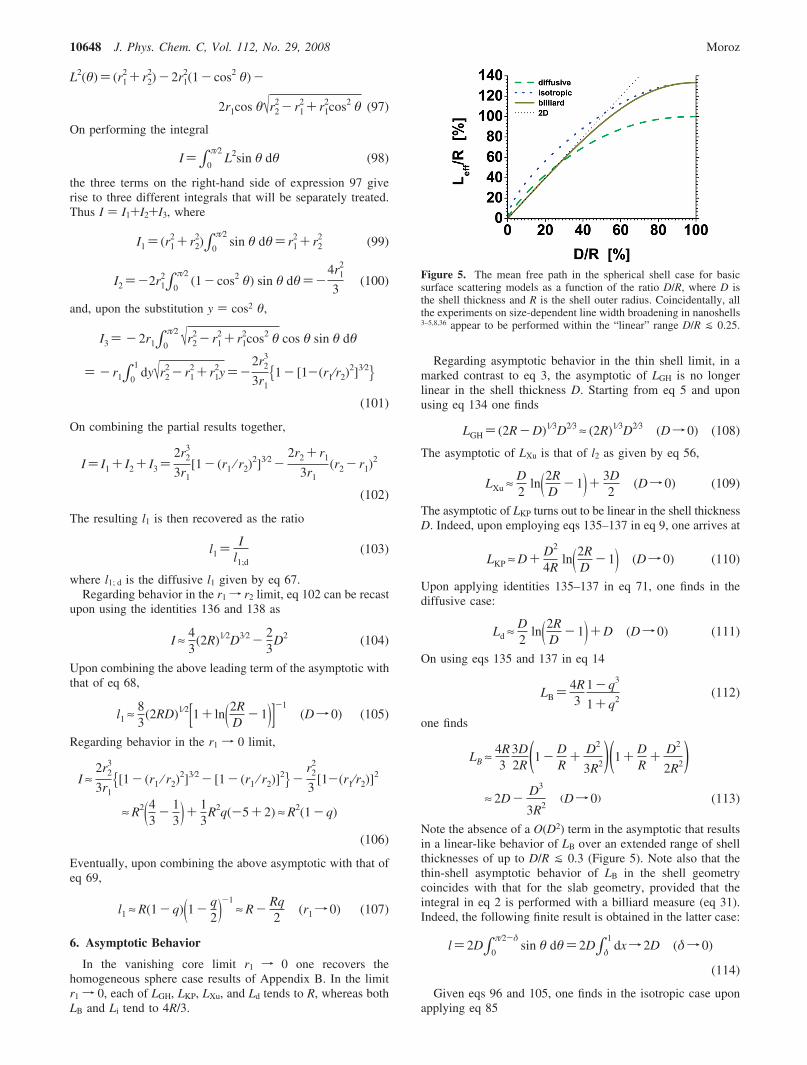
Note the absence of a O(D2) term in the asymptotic that resultsin a linear-like behavior of LB over an extended range of shellthicknesses of up to D/R j 0.3 (Figure 5). Note also that thethin-shell asymptotic behavior of LB in the shell geometrycoincides with that for the slab geometry, provided that theintegral in eq 2 is performed with a billiard measure (eq 31).Indeed, the following finite result is obtained in the latter case:

l) 2D∫0

π⁄2-δsin θ dθ) 2D∫δ

1dxf 2D (δf 0)

(114)

Given eqs 96 and 105, one finds in the isotropic case uponapplying eq 85

Figure 5. The mean free path in the spherical shell case for basicsurface scattering models as a function of the ratio D/R, where D isthe shell thickness and R is the shell outer radius. Coincidentally, allthe experiments on size-dependent line width broadening in nanoshells3–5,8,36 appear to be performed within the “linear” range D/R j 0.25.


Li ≈ 143

(2RD)1⁄2[3+ ln(2RD

- 1)]-1(Df 0) (115)

The leading order of some of the asymptotics could have beensimplified. However, it has been found that by, for example,not neglecting 1 against 2R/D in the logarithm, the resultingasymptotics yield a good approximation to LXu, Ld, and Li in asignificantly larger parameter range.

7. Discussion

A common practice, derived from the homogeneous spherecase, that the mean free path in the shell geometry is proportionalto the shell thickness and that different scattering models onlyaffect the slope of this linear dependence2–5,8 has been demon-strated to be invalid in the spherical shell case. Among thevarious models of surface scattering, the billiard, or Lambertian,model seems to be the most convincing from both purelytheoretical and in view of explaining experimental data. Let ushighlight the following features of the billiard, or Lambertian,surface scattering model:(1) It is the only model that yields a linear behavior of the meanfree path Leff on the shell thickness D in the thin shell limit (upto D/R ≈ 0.3; see Figure 5). Compare that with Ld ≈ (D/2)ln(R/D) in the diffusive case, and with Li ≈ 14(2RD)1/2/[3 ln(R/D)] in the isotropic case (see Section 6 for further details).(2) For any shape of a bounded and connected electron enclosureQ and in any space dimension, the mean free path is straight-forwardly determined by substituting the surface and volumeof Q into eq 10.(3) The billiard measure (eq 31) is the only measure that yieldsa finite result when the integral in eq 2 for the slab geometry isperformed (see eq 114). It goes without saying that the resultcoincides with the thin-shell limit in the spherical shell geometry.(4) Upon using the Birkhoff-Khinchin theorem, the billiardmean free path can be interpreted as the time average of thefree paths along typical trajectories.(5) It appears to agree with quantum-mechanical calculations.(6) It gives the best agreement with the experimental data (seeSection 7.1 below).

Regarding the second feature, in the special case of anarbitrary shape homogeneous convex particle, the geometricformula 10 has been rederived by Coronado and Schatz33 usinga geometrical probability approach, by imposing the conditionthat the resulting probability measure function, on set of all thelines, be invariant under rotation and translation of the threeCartesian coordinates x, y, and z. However, this approach cannotbe used in the present case, because the spherical shell is notof a convex shape.

The third feature can be straightforwardly checked (see eqs2 and 114). The fourth feature is about that the mean free pathis not a simple average over path lengths. Time aspect isimportant as well. The mean free path is rather the time averageof the free path along typical trajectories. The Birkhoff ergodictheorem (see ref 30 and Supporting Information) implies forτ(x) ) L(x)/υp, with υp being the particle velocity, that for almostevery x ∈ M the limit

limNf∞

1N

[L(x)+ ... + L(TN-2x)+ L(TN-1x)]) l(x) (116)

exists. The mean free path Leff is then obtained by averagingl(x) with respect to the probability measure dµB on M,

Leff )∫ l(x) dµB )∫ l(x) dµB (117)

Regarding the fifth feature, the billiard result (eq 141) resultsin the homogeneous sphere case34 when original quantum

mechanical calculation of the dielectric function on using linearresponse theory for a hard sphere model of noninteractingelectrons in an infinitely deep spherical potential well byKawabata and Kubo35 are refined (see also ref 33 for furtherreferences). The only quantum-mechanical calculation in thespherical shell case has been performed by Kraus and Schatz,18

who were able to manage the limiting case of thin shells (seeAppendix 3 in ref 18), and who arrived at eq 118 (see Table 1of ref 18)

Leff ) 2(π ⁄ 3)1⁄3D ≈ 2.0309D (118)

It goes without saying that the quantum-mechanical result almostexactly coincides with the billiard model thin-shell asymptotic(eq 113). However, the latter result has to be taken with caution,as the agreement with the classical asymptotic may be coinci-dental, because a refined Debye asymptotic expansions for large-order Bessel functions were not employed.

7.1 Comparison with Experiment. When measurements areperformed on ensembles of fine metallic particles, the mean freepath Leff is typically determined from the size dependence ofthe imaginary part ε2 of the dielectric constant,13

ε2(ω, R)) ε2b(ω)+ωp

2

ω3

VF

Leff(119)

where ε2b is the size-independent bulk value, and ωp is theplasma frequency. As a rule, the imaginary part of the dielectricconstant is derived by Kramers-Kronig analysis from themeasured absorption spectra. In Figure 7 of ref 13, Kreibigcompared the predictions of the diffusive and isotropic modelsin the homogeneous sphere case against experimental data. [TheKawabata and Kubo quantum-mechanical prediction (labeledas KK line) has already been corrected for a missing 1/π factor;13

according to later refined calculations by Barma and Subrah-manyam,34 the quantum-mechanical prediction should havecoincide with that of the isotropic model displayed as line FPE2in Figure 7.] At a first glance, the comparison appears to favorthe diffusive model over the isotropic model and hence overthe billiard model [the latter two yield identical results in thehomogeneous sphere case (see Appendix B)]. However, aninherent inhomogeneous broadening due to different particlesizes inevitably come into play in studies involving ensemblesof fine nanoparticles. The inhomogeneous broadening leads toan increased apparent value of ε2, which may have resulted ina systematic shift of the observed data from the FPE2 line upto FPE1 line in Figure 7 of ref 13.

In the case of nanoshells, experiments have been, as a rule,mostly focused on the range of thin nanoshells with 0.75 jr1/r2 j 1, which are most interesting from a practical point ofview; they enjoy the largest plasmon red-shift and exhibit thelargest field enhancements. This has also been the case of recentexperiments on single nanoshells performed by Raschke et al.,8

wherein the effective mean free path was investigated forindividual nanoshells with r1 ) 15 nm and with r2 up to 20nm. It has been concluded that the best agreement betweenexperiment and theoretical calculations is found for Leff ) D/Awith A ) 0.5,8 that is, for Leff ) 2D. This behavior for thinshells is exactly that described by the billiard model (see eq109) without any fitting parameter. Indeed, as shown in Section6, the thin shell behavior of LB is, for practical purposes,indistinguishable from its asymptotic LB ≈ 2D for the shellthicknesses of up to D/R j 0.3 (Figure 5). Coincidentally, allthe experiments on size-dependent line width broadening innanoshells3–5,8,36 appear to be performed for D/R j 0.25 and


hence are within the “linear” range. Note that the billiard, orLambertian, scattering model appears to be already singled outby the very linear dependence of Leff on D in the thin shelllimit, because Leff ≈ (D/2) ln(2R/D) in the diffusive case andLeff ≈ 14(2RD)1/2/[3 ln(2R/D)] in the isotropic case (Figure 5).Indeed, all experimental data appear to single out a lineardependence Leff ) D/A.3,4,8

One can probably explain the previously reported values ofA ) 13 and A ) 2 - 34 by a fact that they were found bymeasurements carried out on nanoshell ensembles, and thus inthe presence of an inevitable inhomogeneous broadening.Neglected inhomogeneous distributions of the core/shell ratiomay have led to an overestimation of the surface scattering.Later single particle dark field spectroscopy study of larger goldnanoshells with r1 ≈ 60 nm and r2 ≈ 80 nm by Nehl et al.36

confirmed that ensemble nanoshell extinction spectra are indeedsignificantly broadened by particle size and shape inhomoge-neity. Furthermore, large A parameters may be caused by roughand incomplete gold shells where electrons may additionallyscatter at domain boundaries. Here it is emphasized that,according to the billiard mean free path formula (eq 10), anincrease of the enclosure surface at a constant volume naturallyleads to a decrease in Leff, that is, a larger effective A. Further,roughness and incompleteness of gold shells may also lead toa lift of the energetic degeneracy of orthogonal plasmonpolarizations. This gives rise to an additional contribution toan inhomogeneous broadening of the line width exceeding theinhomogeneity estimated from TEM measurements alone.8

For the nanoshells of ref 36, surface scattering correctionsshould still be feasible (cf eq 1), since the expected mean freepath Leff ≈ 2D ) 40 nm is comparable to l∞ ) 42 nm for gold.13

In spite of that, it has been claimed36 that for some nanoshellsthe line width is even narrower than that obtained with the Mietheory calculation without any account of surface scatteringcorrections. The cause of the narrowing beyond the Mie theorycalculation is currently under investigation, but most probablysome other effects has become important, such as the segregationof impurities close to the surface,16 adsorption substrate matrixeffects,16 or faceting of the nanoshell surfaces.37 Such anarrowing had been reported earlier.37 In the latter case, thenarrowing might be an artifact of the fact that the line widthwas determined from the scattering cross section and not, asusual, from the absorption cross section.16 Contrary to somespeculations,16 the electrical charging of metal nanoparticles onlyshifts the peak position and does not appear to directly influence(only indirectly, via chemisorption)25 the line width of eitherspherical particles25,38 or spheroids.39 Unless nanoshell can beviewed as a porous aggregation of fine metallic clusters, onecan also rule out a structural phase transition, as indicated inthe transition from icosehedral to face-centered cubic (fcc)structure in Au clusters.40 Note additionally that, within theexperimentally tested range of D/R j 0.25, one has Li > Ld >LB (Figure 5). Therefore, the choice of LB as the mean free pathis, even by ignoring its linear asymptotic behavior, still theclosest to the reported experimental data (which occasionallyindicate an apparent mean free path even smaller than LB) andrequires taking into account the minimum of other possibleadditional broadening mechanisms to fully match experimentaldata.

7.2 Theoretical and Practical Implications. The mostpopular choice by far has been, so far, to simply set Leff equalto the shell thickness D.2–5,8 This choice is expected to yieldunrealistically broad homogeneous linewidths. The use of

Kachan and Ponyavina31,32 mean free path LKP (eq 9) does notbring much difference since, for thin shells with r1/r2 ∈ [0.75, 1),one has

0.5LBe LKPj 0.6LB (120)

This is to be expected, because, according to asymptotic (110),LKP ≈ D in the thin shell limit. Therefore, it should only be anegligible difference between using Leff ) Lc ) D and Leff )LKP for thin shells with r1/r2 ∈ [0.75, 1). For the entire range ofshell parameters, one has LB g (4/3)LKP, and the ratio LB/LKP

monotonically increases from 4/3 for q ) r1/r2 ) 0 up to 2 forq ) 1. Therefore, the normalized total decay rates of thefundamental dipole void-like and sphere-like modes of a goldnanoshell are expected to be significantly less affected by surfacescattering than shown in Figure 7 of ref 21. Similarly, thelimitations of ref 10 regarding the experimental feasibility ofproposed multilabel applications of nanoshells by Chen et al.,9

which were established on the basis of Leff ) LKP, are expectedto become much weaker when Leff ) LB is to be used.

On comparing the respective asymptotics of LGH and LB (seeeqs 108 and 113) one finds that, approximately (see also Figure3),

LB < LGH for D ⁄ Rj 1 ⁄ 4LB > LGH for D ⁄ RJ 1 ⁄ 4

(121)

(An exact crossover point is somewhat smaller, namely at 0.23).Consequently, theoretical predictions based on Leff ) LGH willyield unrealistically narrow line width and the quality factor ofthe resonance, Q ) Eres/Γ, for thin shells with D/R j 1/4. Thishas been observed in experiments by Mulvaney and is reportedin Section 9 of ref 25.

Schelm and Smith26,27 took Leff ) LGH/4 as the electroneffective mean free path. Because LGH/4 < LB over allexperimentally feasible range of nanoshell parameters, the limitsof Schelm and Smith27 on resonance tunability in metallicnanoshells can be probably somewhat relaxed, since they wereestablished on assuming too large line width broadening. Forthe same reasons, actual internal electric field densities in andaround metal nanoshells are expected to be somewhat largerthan predicted.26

8. Conclusions

The widely adopted practice that the electron effective meanfree path Leff for thin shells is, irrespective of the underlyingsurface scattering model, proportional to the shell thicknessD,2–5,8 has to be abandoned. Qualitatively different nonlineardependences on the inner and outer shell radii result for differentmodel cases in the shell geometry. This has been confirmed bycalculating the mean free path for the shell geometry under theassumptions of (i) diffusive, (ii) isotropic, and (iii) billiard, orLambertian, scattering.

A comparison with preliminary experimental results onindividual core-shell particles appears to indicate that only thebilliard, or Lambertian, scattering model is compatible with boththe homogeneous sphere and spherical shell case. (The modelpredictions are also compatible with recent experiments onhomogeneous gold nanorods.41) The success of the Eulerdiffusive scattering in the homogeneous sphere case11–14 seemsto be purely accidental, because all the scattering models yielda linear dependence of the mean free path on the sphere radiuswith minor differences in the proportionality factor. A fact thatthe mean free path in the shell geometry is much more sensitiveto underlying model assumptions of electron surface scatteringcan be used in future experiments on single and well-controlled


dielectric core-metal shell nanoparticles (preferably with aconstant total radius R and variable D) in order to test theoreticalpredictions for the full range of nanoparticle parameters, andin particular for D/R j 0.3, that is, outside the “linear” range,in which case deviations from the linear behavior Leff ) 2Dshould become transparent (Figure 5) and thereby discriminatebetween different surface scattering models. This would enableone to more precisely assess the contribution of other mecha-nisms, such as chemical interface damping, to overall plasmonresonance damping. It would be also interesting to performquantum-mechanical calculations in the shell geometry for thefull range of shell parameters. This will be dealt with elsewhere.

Appendix

A

Summary of Elementary Formulas

The law of cosines (also known as the cosine formula or cosinerule),

c2 ) a2 + b2 - 2ab cos θ (122)

where θ is the angle between the sides a and b of a triangleand c is the remaining side opposing the angle.

∫a

bcos θ sin θ dθ)∫cos b

cos ax dx) cos2 a- cos2 b

2(123)

∫a

bcos2 θ sin θ dθ)∫cos b

cos ax2 dx) cos3 a- cos3 b

3(124)

∫ √y2 - 1 dy) 12

(y√y2 - 1- ln|y+ √y2 - 1|) (125)

∫ x dxx- a

) x+ a ln|x- a| (126)

∫ dx(x- a)(b- x)

) 1b- a

ln|x- ab- x | (127)

∫ x2 dx(x- a)(b- x)

) - x- 1b- a

[b2 ln|b- x|-a2 ln|x- a|]

(128)

∫ x dx

√b- x) - 2

3(2b+ x)√b- x (129)

∫ dx

(b- x)3⁄2) 2

√b- x(130)

x2 dx

(b- x)3⁄2) [- (b- x)2

3+ 2b(b- x)+ b2] 2

√b- x

) - 23

(b-x)3⁄2 + 4b√b- x+ 2b2

√b- x

(131)

Here eq 126 is given as eq 1.2.4.13 by ref 42 and can also beeasily verified by differentiation. The identity 127 is given aseq 1.2.7.7 by ref 42 and results from the elementary identity

1(x+ a)(x+ b)

) 1b- a( 1

x+ b- 1

x+ a) (132)

The identity 128 is given as eq 1.2.7.9 by ref 42 and resultsfrom the elementary identity

1(x+ a)(x+ b)

) 1+ 1a- b( b2

x+ b- a2

x+ a) (133)

The identities 129–131 can be derived using eqs 1.2.18.6,1.2.18.9, and 1.2.18.11 of ref 42.

Regarding the thin-shell limit r1 f r2, the following expres-sions have been repeatedly used:

r1 + r2 ) 2R-D (134)

q) 1- DR

(135)

q2 ) (R-D)2

R2) 1- 2D

R+ D2

R2(136)

1

1+ q2≈ 1

2(1+ DR+ D2

2R2) (137)

1r1) 1

R-D≈ 1

R(1+ DR ) (138)

which follow upon writing r1 ) R - D.

B

Homogeneous Sphere

Upon applying the law of cosines (eq 122), one finds for thesphere chord length (cf eq 87)

L(θ)) 2R cos θ (139)

Upon integrating L(θ) with the respective probability measures,eqs 28, 29, and 31, the following mean free paths in the case ofa homogeneous sphere with radius R are obtained:

•In the diffusive case,

Ld )R (140)

i.e., the effective mean free path of the conduction electrons isequal to the homogeneous sphere radius.11

•In the isotropic and billiard cases,13,29

Li ) LB ) 4R ⁄ 3 (141)

The result for Ld follows upon using eq 123, whereas that forLi and LB follows on using eq 124. Note in passing that theequality Li ) LB in the homogeneous sphere case follows fromthe equality dµi ) dµB, which in turn follows upon substitutingeq 139 into eq 29 together with ci ) 1/Ld ) 1/R.

Thus, as established earlier,11–14 the mean free-path in thehomogeneous sphere case is always linearly proportional tothe sphere radius R, irrespective of the assumptions regardingthe electron surface scattering.

Acknowledgment. I thank Professors Chernov, Klar, andMulvaney for discussion.

Supporting Information Available: Intermediary calcula-tion steps are supplied together with the wording of the Birkhoff-Khinchin theorem and an amenable derivation of the billiardformula in its general form (eq 10). This material is availablefree of charge via the Internet at http://pubs.acs.org.

References and Notes

(1) Neeves, A. E.; Birnboim, M. H. J. Opt. Soc. Am. B 1989, 6, 787.(2) Zhou, H. S.; Honma, I.; Komiyama, H.; Haus, J. W. Phys. ReV. B

1994, 50, 12052.(3) Averitt, R. D.; Sarkar, D.; Halas, N. J. Phys. ReV. Lett. 1997, 78,

4217.(4) Westcott, S. L.; Jackson, J. B.; Radloff, C.; Halas, N. J. Phys. ReV.

B 2002, 66, 155431.(5) Grady, N. K.; Halas, N. J.; Nordlander, P. Chem. Phys. Lett. 2004,

399, 167.(6) Hirsch, L. R.; Stafford, R. J.; Bankson, J. A.; Sershen, S. R.; Rivera,

B.; Price, R. E.; Hazle, J. D.; Halas, N. J.; West, J. L. Proc. Natl. Acad.Sci. U.S.A. 2003, 100, 13549.


(7) Loo, C.; Hirsch, L.; Lee, Min-Ho.; Chang, E.; West, J.; Halas, N. J.;Drezek, R. Opt. Lett. 2005, 30, 1012.

(8) Raschke, G.; Brogl, S.; Susha, A. S.; Rogach, A. L.; Klar, T. A.;Feldmann, J.; Fieres, B.; Petkov, N.; Bein, T.; Nichtl, A.; Kurzinger, K.Nano Lett. 2004, 4, 1853.

(9) Chen, K.; Liu, Y.; Ameer, G.; Backman, V. J. Biomed. Opt. 2005,10, 024005.

(10) Khlebtsov, B.; Khlebtsov, N. J. Biomed. Opt. 2006, 11, 044002.(11) Euler, J. Z. Phys. 1954, 137, 318.(12) Kreibig, U.; Fragstein, C. V. Z. Phys. A 1969, 224, 307.(13) Kreibig, U. J. Phys. F: Met. Phys. 1974, 4, 999.(14) Kreibig, U.; Genzel, L. Surf. Sci. 1985, 156, 678.(15) Hovel, H.; Fritz, S.; Hilger, A.; Kreibig, U.; Vollmer, M. Phys.

ReV. B 1993, 48, 18178.(16) Kreibig, U.; Vollmer, M. Optical Properties of Metal Clusters,

Springer Series in Materials Science; Springer: Berlin, 1995.(17) Bohren C. F.; Huffman, D. R. Absorption and Scattering of Light

by Small Particles; John Wiley & Sons: New York, 1998.(18) Kraus, W. A.; Schatz, G. C. J. Chem. Phys. 1983, 79, 6130.(19) Reynolds, F. W.; Stilwell, G. R. Phys. ReV. 1952, 88, 418.(20) Klar, T.; Perner, M.; Grosse, S.; von Plessen, G.; Spirkl, W.;

Feldmann, J. Phys. ReV. Lett. 1998, 80, 4249.(21) Teperik, T. V.; Popov, V. V.; Garcıa, de.; Abajo, F. J. Phys. ReV.

B 2004, 69, 155402.(22) Sander, L. J. Phys. Chem. Solids 1968, 29, 291. As noticed by

Ruppin and Yatom,23 eq 19 should be corrected by a factor of 1/2.(23) Ruppin, R.; Yatom, H. Phys. Status Solidi B 1976, 74, 647.(24) Granqvist, C. G.; Hunderi, O. Z. Phys. B 1978, 30, 47.(25) Mulvaney, P. Langmuir 1996, 12, 788.(26) Schelm, S.; Smith, G. B. J. Phys. Chem. B 2005, 109, 1689.(27) Schelm, S.; Smith, G. B. J. Opt. Soc. Am. A 2005, 22, 1288.

(28) Xu, Hongxing. Phys. ReV. B 2005, 72, 073405.(29) Chernov, N. J. Stat. Phys. 1997, 88, 1.(30) Chernov, N.; Markarian, R. Introduction to the Ergodic Theory of

Chaotic Billiards; http://www.math.uab.edu/chernov/papers/rbook.pdf.(31) Kachan, S. M.; Ponyavina, A. N. Physics, Chemistry and Applica-

tion of Nanostructures: ReViews and Short Notes to Nanomeeting 1999,Minsk, Belarus, May 17-21, 1999; World Scientific: Singapore, 1999; p.103.

(32) Kachan, S. M.; Ponyavina, A. N. J. Mol. Struct. 2001, 563-564,267.

(33) Coronado, E. A.; Schatz, G. C. J. Chem. Phys. 2003, 119, 3926.(34) Barma, M.; Subrahmanyam, V. J. Phys.: Condens. Matter 1989,

1, 7681.(35) Kawabata, A.; Kubo, R. J. Phys. Soc. Japan 1966, 21, 1765. There

should be a factor of 1/π3 in the resulting expressions (4.12) for ε2(ω); cf.eq 10 of ref 13.

(36) Nehl, C. L.; Grady, N. K.; Goodrich, G. P.; Tam, F.; Halas, N. J.;Hafner, J. H. Nano Lett. 2004, 4, 2355.

(37) Sonnichsen, C.; Franzl, T.; Wilk, T.; von Plessen, G.; Feldmann,J. New J. Phys. 2002, 4, 93–1.

(38) Rostalski, J.; Quinten, M. Colloid Polym. Sci. 1996, 274, 648.(39) Mulvaney, P.; Perez-Juste, J.; Giersig, M.; Liz-Marzan, L. M.;

Pecharroman, C. Plasmonics 2006, 1, 61.(40) Kreibig, U. Solid State Commun. 1978, 28, 767.(41) Novo, C.; Gomez, D.; Perez-Juste, J.; Zhang, Z.; Petrova, H.;

Reismann, M.; Mulvaney, P.; Hartland, G. V. Phys. Chem. Chem. Phys.2006, 8, 3540.

(42) Prudnikov, A. P.; Brychkov, Yu. A. Marichev, O. I. Integrals andSeries, 2nd ed; Gordon and Breach: London, 1988.

JP8010074


electron mean free path in a spherical shell geometry · electron mean free path in a spherical...

Documents