electron density functional theory · linear functionals ... g. orbital functionals and optimized...
TRANSCRIPT
Electron Density Functional Theory Page 1
© Roi Baer
Electron Density
Functional Theory
Lecture notes (rough draft)
October 2009
Roi Baer
Institute of Chemistry,
The Fritz Haber Center for Molecular Dynamics
The Hebrew University of Jerusalem,
Jerusalem, 91904 Israel
© Roi Baer
Electron Density Functional Theory Page 2
© Roi Baer
Contents
I. INTRODUCTORY BACKGROUND TOPICS ............................................................. 7
A. THE SCHRÖDINGER EQUATION ....................................................................................... 7
B. BOSONS AND FERMIONS ................................................................................................... 7
I. GROUND-STATE WAVE FUNCTION OF BOSONS .................................................................... 7
II. GROUND-STATE WAVE FUNCTION OF FERMIONS ............................................................. 10
C. WHY ELECTRONIC STRUCTURE IS AN IMPORTANT DIFFICULT PROBLEM .................. 10
D. THE BORN-OPPENHEIMER THEORY ............................................................................. 12
I. THE ADIABATIC THEOREM ................................................................................................. 12
II. MOTIVATION FOR THE BORN-OPPENHEIMER APPROXIMATION: CLASSICAL NUCLEI ....... 16
III. THE BORN-OPPENHEIMER APPROXIMATION IN QUANTUM NUCLEAR CASE .................... 18
E. ELECTRON CORRELATION ............................................................................................. 21
I. THE ELECTRONIC WAVE FUNCTION OF TWO NON-INTERACTING ELECTRONS ................... 21
II. CORRELATION IN ACTION: A WAVE FUNCTION OF 2 INTERACTING PARTICLES IN AN
HARMONIC TRAP ..................................................................................................................... 24
F. THE ELECTRON DENSITY IS A MUCH SIMPLER OBJECT THAN THE WAVE FUNCTION . 31
G. THE VARIATIONAL PRINCIPLE ...................................................................................... 34
H. DILATION RELATIONS .................................................................................................... 36
I. THE CONCEPT OF THE VIRIAL IN CLASSICAL MECHANICS .................................................. 37
II. THE VIRIAL THEOREM IN QUANTUM MECHANICS ............................................................ 39
III. SLATER’S THEORY OF THE CHEMICAL BOND USING THE VIRAL THEOREM ..................... 40
IV. OTHER DILATION FACTS ................................................................................................. 47
I. INTRODUCTION TO FUNCTIONALS ................................................................................. 48
I. DEFINITION OF A FUNCTIONAL AND SOME EXAMPLES ...................................................... 48
II. LINEAR FUNCTIONALS ...................................................................................................... 49
III. FUNCTIONAL DERIVATIVES ............................................................................................. 50
IV. INVERTIBLE FUNCTION FUNCTIONALS AND THEIR FUNCTIONAL DERIVATIVES .............. 53
V. CONVEX FUNCTIONALS ................................................................................................... 54
J. MINIMIZING FUNCTIONALS IS AN IMPORTANT PART OF DEVELOPING A DFT ............ 58
I. MINIMIZATION OF FUNCTIONS ........................................................................................... 58
II. CONSTRAINED MINIMIZATION: LAGRANGE MULTIPLIERS ................................................ 60
III. MINIMIZATION OF FUNCTIONALS .................................................................................... 64
Electron Density Functional Theory Page 3
© Roi Baer
II. MY FIRST DENSITY FUNCTIONAL: THOMAS-FERMI THEORY .................. 68
A. BASIC CONCEPTS IN THE ELECTRON GAS AND THE THOMAS-FERMI THEORY .......... 68
B. MINIMIZATION OF THE THOMAS-FERMI ENERGY ....................................................... 73
C. THOMAS-FERMI DOES NOT ACCOUNT FOR MOLECULES ............................................. 75
D. THOMAS-FERMI SCREENING ......................................................................................... 76
E. VON WEIZSÄCKER KINETIC ENERGY ............................................................................ 80
III. MANY-ELECTRON WAVE FUNCTIONS ............................................................. 81
A. THE ELECTRON SPIN ...................................................................................................... 81
B. THE PAULI PRINCIPLE .................................................................................................... 82
C. THE EXCITED STATES OF THE HELIUM ATOM ............................................................. 83
D. THE SLATER WAVE FUNCTION IS THE BASIC ANTI-SYMMETRIC FUNCTION
DESCRIBING N ELECTRONS IN N ORBITALS .......................................................................... 83
E. WITHOUT LOSS OF GENERALITY, WE MAY ASSUME THE ORBITALS OF A SLATER
WAVE FUNCTION ARE ORTHOGONAL .................................................................................... 84
F. ANY ANTISYMMETRIC FUNCTION CAN BE EXPANDED AS A SUM OF BASIC SLATER
(DETERMINANTAL) FUNCTIONS ............................................................................................. 85
G. DETERMINANT EXPECTATION VALUES ......................................................................... 87
I. ONE-BODY OPERATORS ..................................................................................................... 87
II. TWO-BODY OPERATORS ................................................................................................... 88
IV. THE HARTREE-FOCK THEORY ........................................................................... 89
A. THE HARTREE-FOCK ENERGY AND EQUATIONS ......................................................... 89
B. RESTRICTED CLOSED-SHELL HARTREE-FOCK ............................................................ 95
C. ATOMIC ORBITALS AND GAUSSIAN BASIS SETS ........................................................... 98
D. VARIATIONAL-ALGEBRAIC APPROACH HARTREE-FOCK ........................................... 99
E. THE ALGEBRAIC DENSITY MATRIX AND CHARGE ANALYSIS................................... 105
F. SOLVING THE HARTREE-FOCK EQUATIONS ............................................................... 107
I. DIRECT INVERSION IN ITERATIVE SPACE (DIIS) .............................................................. 107
II. DIRECT MINIMIZATION .................................................................................................. 108
G. PERFORMANCE OF THE HARTREE-FOCK APPROXIMATION ..................................... 109
Electron Density Functional Theory Page 4
© Roi Baer
H. BEYOND HARTREE-FOCK ............................................................................................ 110
V. ADVANCED TOPICS IN HARTREE-FOCK THEORY ....................................... 112
A. LOW-LYING EXCITATIONS AND THE STABILITY OF THE HARTREE-FOCK GROUND
STATE .................................................................................................................................... 112
I. CI-SINGLES AND BRILLOUIN’S THEOREM ....................................................................... 112
II. HARTREE-FOCK STABILITY ............................................................................................ 114
B. KOOPMANS’ THEOREM ................................................................................................ 116
C. FRACTIONAL OCCUPATION NUMBERS, THE HF ORBITAL FUNCTIONAL AND THE
GENERALIZED KOOPMANS’ THEOREM ............................................................................... 119
D. HARTREE-FOCK FOR THE HOMOGENEOUS ELECTRON GAS ...................................... 121
I. HARTREE-FOCK ORBITALS AND ORBITAL ENERGIES OF HEG ......................................... 121
II. THE DENSITY OF STATES OF THE HEG ........................................................................... 127
III. STABILITY OF THE HEG IN HARTREE-FOCK THEORY ................................................... 129
VI. THE HOHENBERG-KOHN DENSITY THEORY ............................................... 131
A. THE FIRST HK THEOREM ............................................................................................ 131
B. THE HK FUNCTIONAL .................................................................................................. 133
C. MINIMUM PRINCIPLE FOR DENSITY FUNCTIONAL THEORY ...................................... 135
D. AN INTERESTING OBSERVATION ON THE VARIATIONAL PRINCIPLE OF NON-
INTERACTING ELECTRONS ................................................................................................... 137
E. THE SET OF V-REPRESENTABILE DENSITIES ............................................................... 138
I. V-REP DENSITIES CORRESPOND TO GROUND STATES WAVE FUNCTION OF SOME POTENTIAL
WELL ...................................................................................................................................... 138
II. SOME NON-V-REPRESENTABILIT ISSUES ......................................................................... 139
III. THE SET OF V-REP DENSITIES OF A GIVEN ELECTRON NUMBER IS NOT CONVEX ........... 140
F. LEVY-LIEB GENERALIZATION OF THE HK FUNCTIONAL .......................................... 143
G. THE DILATION INEQUALITY FOR THE HK FUNCTIONAL ........................................... 148
VII. THE KOHN-SHAM METHOD .............................................................................. 149
A. NON-INTERACTING ELECTRONS .................................................................................. 149
Electron Density Functional Theory Page 5
© Roi Baer
B. ORBITALS FOR THE NON-INTERACTING ELECTRONS ................................................. 153
C. THE CORRELATION ENERGY FUNCTIONAL: DEFINITION AND SOME FORMAL
PROPERTIES .......................................................................................................................... 154
D. THE KOHN SHAM EQUATIONS ..................................................................................... 157
I. THE KOHN-SHAM EQUATION FROM A SYSTEM OF NON-INTERACTING PROBLEM ........... 157
II. SYSTEMS WITH PARTIALLY OCCUPIED ORBITALS ........................................................... 159
III. IS THE GROUND STATE WAVE FUNCTION OF NON-INTERACTING PARTICLES ALWAYS A
SLATER WAVE FUNCTION ...................................................................................................... 161
IV. JANAK’S THEOREM ....................................................................................................... 163
E. “VIRIAL THEOREM” RELATED IDENTITIES IN DFT ................................................... 164
F. GALILEAN INVARIANCE................................................................................................ 168
G. HOLES AND THE ADIABATIC CONNECTION ................................................................. 170
I. THE EXCHANGE AND CORRELATION HOLES .................................................................... 170
II. THE FERMI-COULOMB HOLE FOR HARMONIC ELECTRONS ............................................. 175
III. THE FERMI HOLE IN THE NON-INTERACTING SYSTEM ................................................... 178
IV. THE ADIABATIC CONNECTION ...................................................................................... 181
H. DERIVATIVE DISCONTINUITY IN THE EXCHANGE CORRELATION POTENTIAL
FUNCTIONAL ......................................................................................................................... 184
VIII. APPROXIMATE CORRELATION ENERGY FUNCTIONALS ..................... 185
A. THE LOCAL DENSITY APPROXIMATION (LDA) ........................................................... 185
I. THE EXCHANGE ENERGY PER ELECTRON IN THE HEG .................................................... 186
II. CORRELATION ENERGY OF THE HEG: THE HIGH DENSITY LIMIT ................................... 187
III. CORRELATION ENERGY OF THE HEG: THE LOW DENSITY LIMIT AND THE WIGNER
CRYSTAL ................................................................................................................................ 189
IV. MONTE-CARLO DETERMINATION OF THE CORRELATION ENERGY FOR THE HEG ........ 192
V. THE POLARIZED HEG; LOCAL SPIN-DENSITY APPROXIMATION (LSDA) ....................... 192
VI. SUCCESSES AND FAILURES OF LSDA ............................................................................ 193
VII. PLAUSIBLE REASONS FOR THE SUCCESS OF LSDA ...................................................... 193
B. SEMILOCAL FUNCTIONALS AND THE GENERALIZED GRADIENT APPROXIMATION .. 196
IX. GENERALIZED KOHN-SHAM APPROACHES ................................................. 196

Electron Density Functional Theory Page 6
© Roi Baer
A. THE GENERALIZED KOHN-SHAM FRAMEWORK ........................................................ 196
B. KOHN-SHAM FROM GENERALIZED KS ....................................................................... 199
C. THE HYBRID FUNCTIONAL OF BECKE ........................................................................ 199
D. ........................................................................................................................................... 200
E. LONG-RANGE SELF-REPULSION AND LACK OF DERIVATIVE DISCONTINUITY .......... 200
F. RANGE SEPARATED HYBRIDS ....................................................................................... 200
G. ORBITAL FUNCTIONALS AND OPTIMIZED EFFECTIVE POTENTIALS .......................... 200
H. APPROXIMATE CORRELATION FUNCTIONALS AND THE BORN-OPPENHEIMER FORCE
ON NUCLEI............................................................................................................................. 200
X. MORE ON THE DFT CORRELATION ENERGY ................................................ 203
A. APPROXIMATIONS TO EX ARE APPROXIMATION TO EC ............................................. 203
B. THE NECESSITY OF LONG-RANGE PARAMETER TUNING ............................................ 209
I. THE SYMMETRIC RADICAL CATION ................................................................................. 209
II. AROMATIC DONOR -TCNE ACCEPTOR CHARGE TRANSFER EXCITATION ....................... 211
XI. TDDFT ........................................................................................................................ 214
A. TIME-DEPENDENT LINEAR RESPONSE THEORY ......................................................... 214
B. ALGEBRAIC APPROACH TO LINEAR RESPONSE .......................................................... 216
C. FREQUENCY-DOMAIN RESPONSE ................................................................................. 219
D. EXCITATION ENERGIES FROM THE ALGEBRAIC TREATMENT ................................... 220

Electron Density Functional Theory Page 7
© Roi Baer
I. Introductory background topics
A. The Schrödinger equation
XXX
B. Bosons and Fermions
i. Ground-state wave function of Bosons
Consider a one dimensional Schrödinger equation for the ground state, which
may be taken real. We will ask: is this wave function of the same sign
everywhere? What we mean is: is it all non‐negative or all non positive? Of
course, if it is all non‐positive then we can multiply it by ‐1 and ask again: is it
all non‐negative? Saying it is of a constant sign is the same as saying it has no
nodes, i.e. it does not go through the x‐ axis anywhere.
Exercise: Prove the following theorem:
Theorem: The ground‐state wave function of a 1D wave non‐degenerate
Schrödinger equation has no nodes.
Proof. Let us assume is the (real) normalized ground state. Then it is the
wavefunction minimizes the functional:
(1.1.1)
A robust expression for the kinetic energy expectation value
The kinetic energy is usually defined as . Let us
call this . For continuous and twice differentiable functions that go to zero at
∞ an equivalent definition, is | | . Let us call this
Electron Density Functional Theory Page 8
© Roi Baer
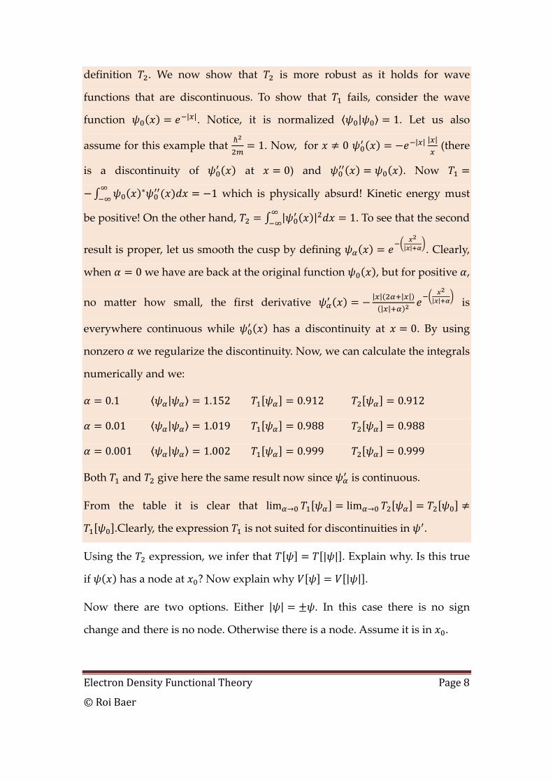
definition . We now show that is more robust as it holds for wave
functions that are discontinuous. To show that fails, consider the wave
function | |. Notice, it is normalized | 1. Let us also
assume for this example that 1. Now, for 0 | | | | (there
is a discontinuity of at 0) and . Now
1 which is physically absurd! Kinetic energy must
be positive! On the other hand, | | 1. To see that the second
result is proper, let us smooth the cusp by defining | | . Clearly,
when 0 we have are back at the original function , but for positive ,
no matter how small, the first derivative | | | || |
| | is
everywhere continuous while has a discontinuity at 0. By using
nonzero we regularize the discontinuity. Now, we can calculate the integrals
numerically and we:
0.1 | 1.152 0.912 0.912
0.01 | 1.019 0.988 0.988
0.001 | 1.002 0.999 0.999
Both and give here the same result now since is continuous.
From the table it is clear that lim lim
.Clearly, the expression is not suited for discontinuities in .
Using the expression, we infer that | | . Explain why. Is this true
if has a node at ? Now explain why | | .
Now there are two options. Either | | . In this case there is no sign
change and there is no node. Otherwise there is a node. Assume it is in .

Electron Density Functional Theory Page 9
© Roi Baer
Let us compute the energy change when one makes a small perturbation to
| |:
| | | | 2 | | | | | | (1.1.2)
Verify this and show we explicitly assumed that the norm of is 1.
Assume the node is at 0 so the wave function changes sign there.
Figure I‐1: The absolute value of the wave function and the parabola in it.
We plot in Figure I‐1 a typical situation. We determine a large enough
parameter and the parabola:
12
which has the properties that it is tangent at some and to | | (and
where ). Then one defines a new wave function:
| | (1.1.3)
By increasing the parabola becomes narrow; adjusting accordingly we
can cause and to uniformly approach 0 as close as needed. Under these
conditions, it is possible to show that
X1 X2
|ψ|
g(x)
Electron Density Functional Theory Page 10
© Roi Baer
| 0 |
12 | 0 |
Now, . One power of comes from integration over the
interval of length where the two functions differ. The second power
comes from the difference . The kinetic energy
difference is negative: . As ∞ the total change in
energy is dominated by the change in the kinetic energy and is thus negative,
showing that | | . This is a contradiction, since is assumed
the ground state. ♦
The proof can be extended to any number of dimensions. It can be used to
prove that the ground state of a many‐boson wave function has no nodes.
Prove an important immediate corollary from this theorem: the ground state
of boson systems is non‐degenerate.
ii. Ground-state wave function of Fermions
XXX
C. Why electronic structure is an important
difficult problem
In this course, we will study methods to treat electronic structure. This
problem is often considerably more complicated than nuclear dynamics of
molecules. The most obvious reason is that usually there are many more
electrons than nuclei in a molecule. However, there are more reasons:
electrons in molecules have extreme ʺquantum mechanicalʺ character, while
nuclei are more ʺclassicalʺ. This last statement requires probably some
Electron Density Functional Theory Page 11
© Roi Baer
explanation. We will discuss in this course ways of mapping the electrons in a
molecule onto a system of non‐interacting particles. In such a picture, each
electron ʺhasʺ its own orbital or wave‐function. Generally, the orbitals of
different electrons in molecules strongly overlap. Furthermore, most of the
valence orbitals are widely spread over space, encapsulating many molecular
nuclei. Nuclei on the other hand, are massive, so their wave functions are
strongly localized and hardly overlap once again, they behave much more
like classical particles.
Describing electronic structure is therefore a quantum mechanical problem.
Now, the electrons interact, via the attractive Coulomb force, not only with
the stationary nuclei but also with each other: each electron repels each other
electron via the repulsive Coulomb force. This makes the electronic structure
problem a many‐body problem.
Quantum many‐body problems are very difficult to track down, much more
difficult than classical mechanical ones. The reason is that for eN electrons
the many‐body wave function is then a function of 3 eN variables, ( )1... eNψ r r ,
where ir (i=1… eN ) is 3 dimensional the position vector. Highly accurate
numerical representation of such functions is next to impossible for 1eN > .
Thus, electronic structure methods invariably include approximate methods.
Typically, the wave function encapsulates much more information than we
care to know about. For example, ( )23 3
1 1,...,e eN Nd r d rψ r r gives the
probability for finding an electron at 1r and an electron at 2r and an electron at
3r etc. Indeed, the total probability is 1:
, … , … 1 (1.3.1)
Electron Density Functional Theory Page 12
© Roi Baer
D. The Born-Oppenheimer theory
i. The adiabatic theorem
Suppose a Hamiltonian is dependent parameterically on , , … . We
write this as . Denote the eigenstates of this Hamiltonian by
(1.4.1)
Now, suppose we change with time, so that we have a trajectory, . The
Hamiltonian will become time dependent: . Suppose the
system is placed in its ground state at time 0, 0 0 . It will
evolve according to the TDSE:
(1.4.2)
Now, the adiabatic theorem says that if changes very slowly then:
(1.4.3)
Namely, except for a purely TD phase, the evolving state stays the
instantaneous ground state of the Hamiltian .
To show this, we use the instantaneous eigenstates to expand :
(1.4.4)
We want to plug this expansion into the SE. So let us calculate:
(1.4.5)
And:
Electron Density Functional Theory Page 13
© Roi Baer
(1.4.6)
Equating the two expressions gives:]
0 (1.4.7)
Now let us multiply by and integrate (remember that | ):
0 (1.4.8)
Now, we have:
0 | (1.4.9)
And since , we find:
(1.4.10)
The matrix is the matrix of “time‐dependent non‐adiabatic
couplings (TDNACs)” and it is an anti‐Hermitean matrix. Furthermore, for
0 (1.4.11)
Thus:
(1.4.12)
We see creates the non‐adiabatic transitions, i.e. the transitions out of the
groud state.
Let us play a bit with . Take the time derivative of the TISE:
Electron Density Functional Theory Page 14
© Roi Baer
(1.4.13)
Multiply by | and get:
| | . (1.4.14)
Since: | we have:
| . (1.4.15)
If then:
. (1.4.16)
This is called the Hellmann‐Feynman theorem, showing that the power is the
expectation value of the rate of change of the Hamiltonian. If :
. (1.4.17)
This is called Epstein’s theorem, giving an expression for the TDNACs.
Remember that depends on through the positions of the nuclei.
Thus:
∂∂RN
(1.4.18)
Thus:
RN (1.4.19)
where:
RN (1.4.20)
Electron Density Functional Theory Page 15
© Roi Baer
We see that the TDNACs depend on the velocity of the nuclei. When nuclei
are small the couplings out of the ground state are small. The are called
the “non‐adiabatic couplings (NACs)”. We find that as long as are not
zero on the trajectory, one can always find small enough that makes the
TDNACs as small as we wish. All we need for states and to stay
decoupled is for the following conditions to be met:
| | 1 (1.4.21)
Thus we can make the NACs small. So all that is left in Eq. (1.4.12) is
. Define the non‐dynamical phase as: (note
is real) and then:
. (1.4.22)
The total state is
(1.4.23)
where is called the dynamic phase. It is easy to prove
that if traverses a closed loop, the non‐dynamical phase depends only on
that loop and not on the way it is traversed. For example, if we traverse the
same loop using different velocities, the dynamic phase may change but the
geometric phase will not. The closed loop geometric angle is called the Berry
phase. The independence of path is a result of the fact that the non‐dynamical
phase is a line integral, and can be made with no reference to time:
Electron Density Functional Theory Page 16
© Roi Baer
(1.4.24)
The dynamical phase for example is not a line integral and its value depends
not only on the path itself but also on the velocity taken along the way. This
observation makes the non‐dynamical phase a special quantity. Berry has
shown that this quantity can give us information on the way the Hamiltonian
is dependent on its parameters. For a real Hamiltonian, for example
around a closed path always equals either 1 or ‐1. If there is an even number
of degeneracies enclosed by the path it is 1 and if an odd number – it is ‐1.
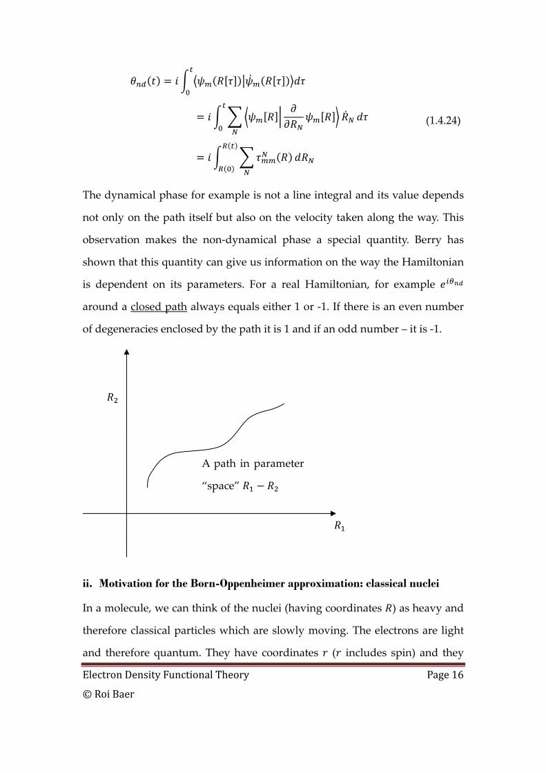
ii. Motivation for the Born-Oppenheimer approximation: classical nuclei
In a molecule, we can think of the nuclei (having coordinates ) as heavy and
therefore classical particles which are slowly moving. The electrons are light
and therefore quantum. They have coordinates ( includes spin) and they
A path in parameter
“space”
Electron Density Functional Theory Page 17
© Roi Baer
feel the effect of slowly moving nuclei. The electron dynamics is controlled by
the Hamiltonian:
, . (1.4.25)
The potential , describes the Coulombic interactions between electrons
and nuclei (in atomic units):
,,
12
1 12 . (1.4.26)
In general, one wants to assume that the total energy of the molecule in this
classical approximation is:
(1.4.27)
Where is the ground state of the electrons at nuclear configuration .
The adiabatic theorem states that this is reasonable as long as nuclei move
slowly. Thus, the adiabatic theorem allows us to write:
(1.4.28)
where is the ground state energy of the electrons at nuclear
configuration . This energy is a usual classical mechanical energy and the
Newton equations of motion apply:
(1.4.29)
We see, that the adiabatic theorem allows us to consider the nuclei as moving
in a potential well which is essentially the eigensvalue of the electrons. This in
essence is the BO approximation when the nuclei are classical.
Electron Density Functional Theory Page 18
© Roi Baer
iii. The Born-Oppenheimer approximation in quantum nuclear case
The classical approach motivates a quantum treatment. We are expecting that
nuclei will not excite electrons very efficiently. That is the motivation for the
BO approximation.
The Born and Oppenheimer development is similar to that of the adiabatic
theorem, although there are no “external” fields. Suppose we have a system of
fast particles, with coordinates , , … and slow particles, with
coordinates , , … . The Hamiltonian can be written as:
, (1.4.30)
The Schrödinger equation is:
, , (1.4.31)
Note that we can assume these wave functions are orthogonal:
| , , (1.4.32)
Now, to proceed, let us first consider the fast r‐Hamitonian
, (1.4.33)
In this “fast Hamiltonian” , the slow variables are simply parameters (it
contains no derivatives with respect to ). Thus, it depends on
parametrically. The fast eigenavalue problem is:
; ; (1.4.34)
The eigenvalues are functions of the parameters . They are called the
adiabatic (or Born‐Oppenheimer) surfaces. The notation with the semicolon
between and is designed to emphasize that are wave functions in but
they depend only parametrically on . This means, for example that the
Electron Density Functional Theory Page 19
© Roi Baer
overlap of the fast eigenstates (called adiabatic states) involves integration
only over , the dynamical coordinates, while is held fixed, since it is only a
parameter:
; ; (1.4.35)
We cannot in fact say anything really meaningful about when
(except when is infinitesimal, but we will not go into this issue
here). Now, we can expand the “real” wave‐function as a linear combination
of the adiabatic functions:
, ; Φ (1.4.36)
We can do this because for any give ; span the space of wave
functions dependent on . In fact, the expansion coefficients, Φ are given
by:
Φ ; , (1.4.37)
Now, let us plug Eq. (1.4.36) into the SE (1.4.31):
, ,
; Φ ; Φ (1.4.38)
Note that, since ∑ where: . We have:
; Φ
Φ ;1
; Φ
; Φ
(1.4.39)
Electron Density Functional Theory Page 20
© Roi Baer
Multiplying Eq. (1.4.38) by ; and integrating over gives:
A Φ Φ Φ (1.4.40)
Where:
A ; ;
; ;
(1.4.41)
The matrices are the non‐adiabatic couplings in the “fast”
system. These are exactly the non‐adiabatic coefficients in the adiabatic theory
(Eq. (1.4.20)).
It is possible to show that:
A Φ Φ
2 Φ (1.4.42)
Thus Eq. (1.4.40) becomes:
2 Φ Φ Φ (1.4.43)
This is a Schrödinger –like equation which determines the coefficients Φ .
These are called the “slow eigenfunctions”. Once they are computed one has
an exact solution to the Schrödinger equation. However, we do not really
want to solve this infinite set of coupled differential equations. Thus we
assume that the quantities for can be neglected. Note that here there
Electron Density Functional Theory Page 21
© Roi Baer
is no which can be taken as small as needed to make the effect of as
minute as we need. Still we can jope that the fact that we chose to be slow
degrees of freedom allow us to make just this approximation! This was the
idea of Born and Oppenheimer who neglected :
2 Φ Φ Φ (1.4.44)
The resulting equation is a Schrödinger equation for the slow degrees of
freedom, which move under the force of electrons derived from a potential
. When applied to molecules the slow degrees of freedom are usually
the nuclei and the fast ‐ the electrons. . There is a problem with neglecting
because of their non‐dynamical effect. Taking them into account results in
treating them as a magnetic field:
2 Φ Φ Φ (1.4.45)
The BO approximation breaks the molecular SE into two consecutive tasks.
First, the electronic SE Eq. (1.4.34) must be solved for any relevant clamped
position of nuclei . Then, the nuclear equation (1.4.26).
Further reading on this subject: M. Baer, Beyond Born‐Oppenheimer:
electronic non‐adiabatic coupling terms and conical intersections (Wiley,
Hoboken, N.J., 2006).
E. Electron correlation
i. The electronic wave function of two non-interacting electrons
In order to appreciate the complexity of the electronic wave function, let us
first study a simple system, of two non‐interacting electrons in a 1D ʺatomicʺ
Electron Density Functional Theory Page 22
© Roi Baer
well. We consider an atomic well given by the potential and we place
in it an electron. The Hamiltonian is:
2 (1.5.1)
Now consider a 2‐electron problem. Assume we have two electrons,
Fermions, which are non‐interacting in the well. The Hamiltonian is
1 2 (1.5.2)
The notation means the Hamiltonian of Eq. (1.5.1) with the coordinate of
the i‐th electron.
What are the eigenstates in this case? First, since each electron can have a
spin, we must decide on the spin of the state. For now, let us assume the state
is spin‐polarized, i.e. that the total spine is 1, both electrons are in spin‐up
orbitals. We try the following form as a wave function:
Ψ ,1√2
1 2 (1.5.3)
Notice that the spatial part is anti‐symmetric while the spin part is symmetric.
This renders the entire wave‐function anti‐symmetric, in accordance with the
Pauli principle. The notation 1 2 means both electrons have spin
projection up . We do not yet know if and under what conditions this wave
function can actually describe eigenstates of the two electrons the
Hamiltonian (1.5.2). We assume that and are orthonormal. This
makes the state normalized, since:
Electron Density Functional Theory Page 23
© Roi Baer
Ψ ,12
12
2
(1.5.4)
The first and second terms are both equal to:
1 1
1 (1.5.5)
The third term in (1.5.4) is:
0 0 0 (1.5.6)
Indeed the entire wave function is orthonormal (thanks to the factor 1/√2 in
(1.5.3)).
Now, let us see under what condition the wave function in Eq. (1.5.3) is an
eigenstate of the Hamiltonian in (1.5.2)
Ψ , 1 2 Ψ ,
1√2
1 2
1√2
1 2
(1.5.7)
This should be equated to:
Ψ ,1√2
(1.5.8)
If we choose the orbitals and to be eigenstates of h (which are
orthogonal so that is compatible with our previous assumption):
Electron Density Functional Theory Page 24
© Roi Baer
, 0,1, … (1.5.9)
Thus:
Ψ ,1√2
1√2
Ψ ,
(1.5.10)
And we see that indeed Ψ , is an eigenstate with energy
.
ii. Correlation in action: a wave function of 2 interacting particles in an
Harmonic trap
We now build a simple electronic structure model that will allow us to study
in some detail the most basic concepts. For this, we suppose that the electrons
are in a harmonic atom, that is the potential well:
12 (1.6.1)
The two lowest eigenstates of a Harmonic oscillator are:
(1.6.2)
The normalization constants are:
/,
4 /
(1.6.3)
And the eigenvalues are:
12 , 0,1, … (1.6.4)
Electron Density Functional Theory Page 25
© Roi Baer
The groundstate energy of the 2‐electron system in the triplet state will be
placing one electron in and another in :
2 (1.6.5)
As discussed above singlet and triplet two‐electron ground state wave
functions composed of two orbitals must be space‐symmetric or
antisymmetric, respectively. We consider below 3 wave functions. The first
Ψ , is the ground state singlet where both electrons are in . The second
and third are a singlet and a triplet made from one electron in and the
other in :
ΨS, ,
ΨS, ,1√2
ΨT, ,1√2
(1.6.6)
The normalization factors are:
1√2
(1.6.7)
Eq. (1.6.6) describes the distribution of positions of both electrons in their
corresponding states. We now want to ask, how much are the electrons in this
state aware of each other? Do they correlate their motion in some way? One
way to measure correlation is to consider the quantity . If
electrons are completely unaware of each other, this quantity, called the
position‐autocorrelation function is zero because then the average of the
product of their position must decompose to the product of the average. Any

Electron Density Functional Theory Page 26
© Roi Baer
deviance from zero indicates some degree of correlation. For the triplet wave
function in Eq. (1.6.6) we find:
Ψ , | |Ψ ,12
| |
12
| | | | | |
| | | | | |12
| | | | 0
(1.6.8)
Of‐course, the same result would be obtained if we calculate because the
electrons are equivalent. Furthermore:
Ψ , | |Ψ ,12
| |
12
| | | | | | | |
| | | | | | | |
| | | |12
(1.6.9)
This negative quantity is there because the Pauli principle pushes the
electrons to opposite sides (when one electron has positive x coordinate the
other has negative and vice versa). Let’s see what happens in the singlet wave
function Ψ , . Here too 0. Then:
Ψ , | |Ψ , | |
| | | | 0 (1.6.10)
Thus, the singlet ground state shows no correlation. However, this does not
mean that all singlet wave functions of 2 electrons have no correlation.
Indeed, let us study the situation in Ψ , . The development is very similar to
Eq. (1.6.9), except that the minus sign is now a plus sign so:
Electron Density Functional Theory Page 27
© Roi Baer
Ψ , | |Ψ ,12
| |
| | | |12
(1.6.11)
Here we find positive autocorrelation, indicative of the fact that spin‐opposite
non‐interacting pairs of electrons want to stick together (when one has
positive x the other wants to have as well and when one has negative the
other one wants negative as well) like non‐interacting bosons.
Since there is no interaction between the electrons, the correlation in these
wave functions arises only from the Pauli principle, i.e. because we impose
the fact that electrons are Fermions. This is called Fermi correlation. Our
lesson is this:
1) Wavefunctions that are mere products of singe‐particle orbitals have no correlation. 2) If the products are symmetrized like in the case of the excited singlet the correlation
is positive indicating that the particles “like to be together” i.e. both on the right or both on the left of the origin.
3) If the products are anti‐symmetrized like in the case of the triplet the correlation is negative indicating that the particles “like to be seperated”.
Up to now, we assumed no e‐e interaction. So now let’s include it and add to
the Hamiltonian an interaction term:
1 2 , (1.6.12)
Let us take one case of coupling which is simple enough to yield to analytical
analysis:
, (1.6.13)
With . This interaction seems strange at first site because it does not
depend on the distance between the particles, as we are used to from
electrostatics, yet, it does describe a repulsion: since if and are both large
and of the same sign this is energy‐costly; if they are both large and of
opposite sign that lowers energy. In this case, the Hamiltonian is:
Electron Density Functional Theory Page 28
© Roi Baer
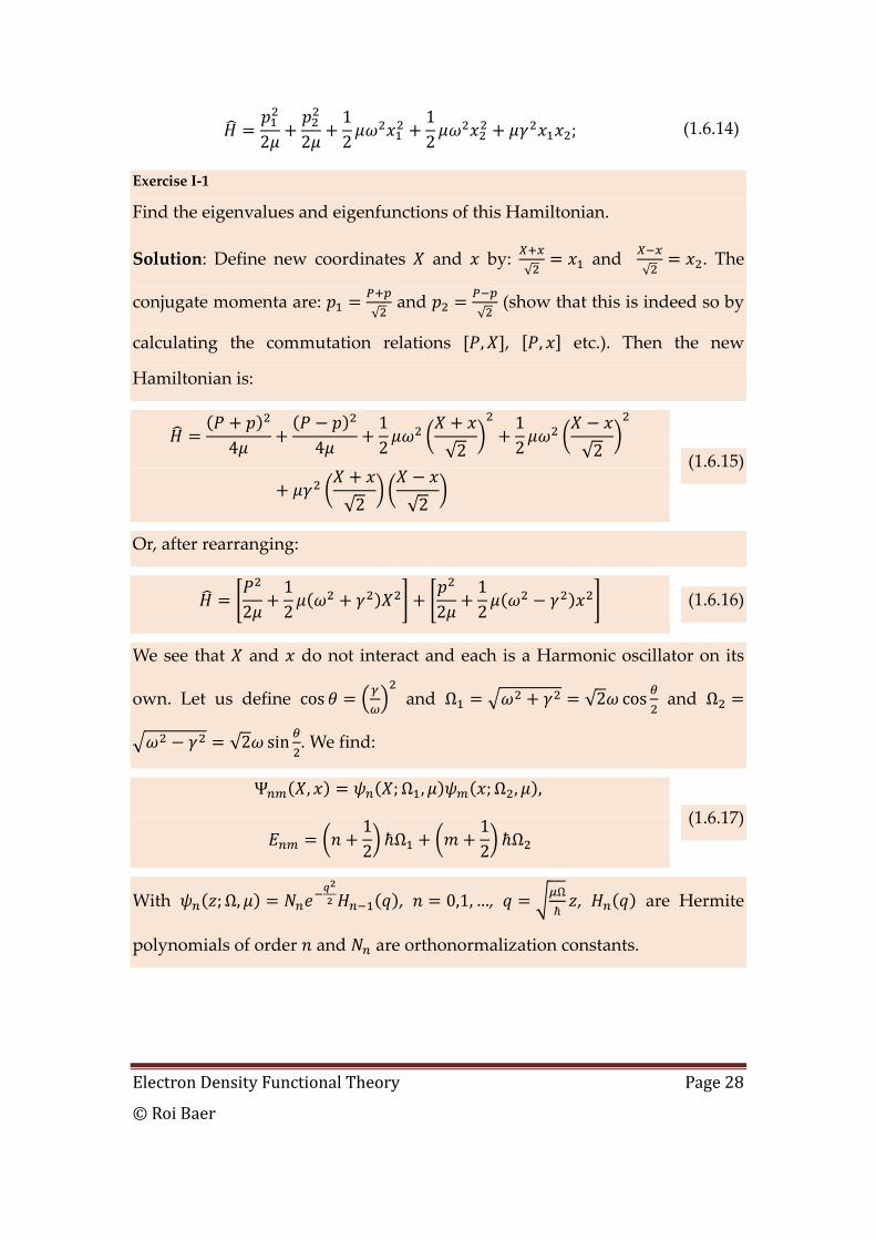
2 212
12 ; (1.6.14)
Exercise I‐1
Find the eigenvalues and eigenfunctions of this Hamiltonian.
Solution: Define new coordinates and by: √
and
√. The
conjugate momenta are: √ and
√ (show that this is indeed so by
calculating the commutation relations , , , etc.). Then the new
Hamiltonian is:
4 412 √2
12 √2
√2 √2
(1.6.15)
Or, after rearranging:
212 2
12 (1.6.16)
We see that and do not interact and each is a Harmonic oscillator on its
own. Let us define cos and Ω √2 cos and Ω
√2 sin . We find:
Ψ , ; Ω , ; Ω , ,
12 Ω
12 Ω
(1.6.17)
With ; Ω, , 0,1, …, Ω , are Hermite
polynomials of order and are orthonormalization constants.
Electron Density Functional Theory Page 29
© Roi Baer
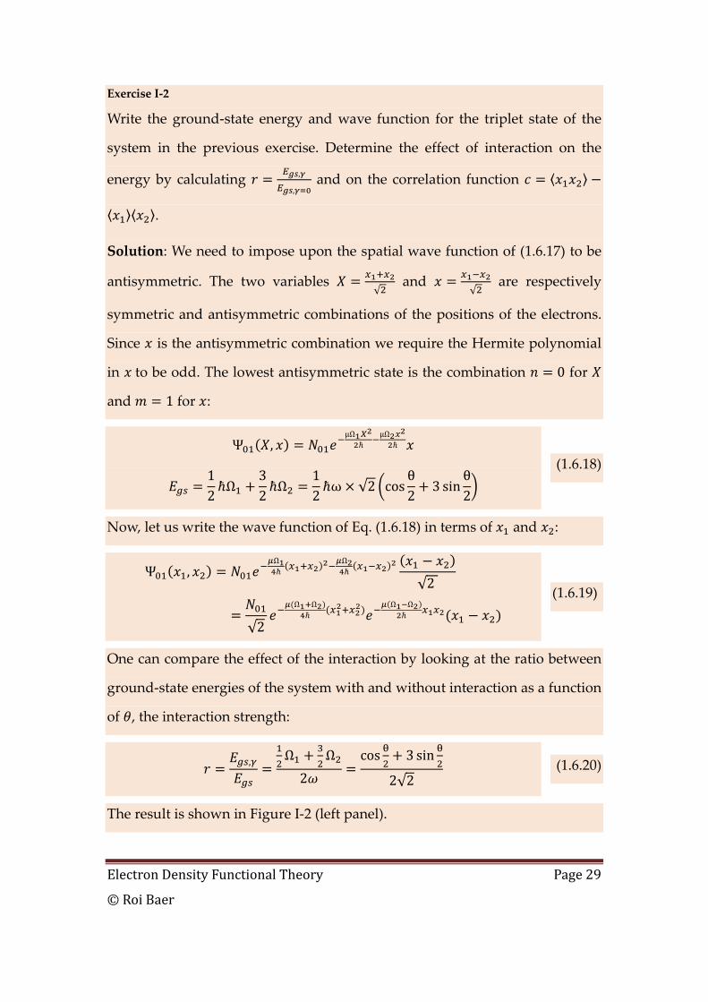
Exercise I‐2
Write the ground‐state energy and wave function for the triplet state of the
system in the previous exercise. Determine the effect of interaction on the
energy by calculating ,
, and on the correlation function
.
Solution: We need to impose upon the spatial wave function of (1.6.17) to be
antisymmetric. The two variables √ and
√ are respectively
symmetric and antisymmetric combinations of the positions of the electrons.
Since is the antisymmetric combination we require the Hermite polynomial
in to be odd. The lowest antisymmetric state is the combination 0 for
and 1 for :
Ψ ,µΩ µΩ
12 Ω
32 Ω
12 ω √2 cos
θ2 3 sin
θ2
(1.6.18)
Now, let us write the wave function of Eq. (1.6.18) in terms of and :
Ψ ,Ω Ω
√2
√2
Ω Ω Ω Ω
(1.6.19)
One can compare the effect of the interaction by looking at the ratio between
ground‐state energies of the system with and without interaction as a function
of , the interaction strength:
, Ω Ω2
cos 3 sin
2√2 (1.6.20)
The result is shown in Figure I‐2 (left panel).

Electron Density Functional Theory Page 30
© Roi Baer
Figure I‐2: (Left panel) The ratio , / ; (Right panel) the correlation ratio /
vs interaction strengths
The interaction lowers the energy, because now the wave function can acquire
a structure that promotes the electrons being away from each other. Thus one
is pushed towards the direction and the other towards that of and thus
they acquire a large negative value of . To see this note that the
expectation values of and are both zero and therefore and are
zero as well. Furthermore note that 2 and the auto‐correlation
is:
12 (1.6.21)
The expectation value of the square position in harmonic oscillator is easily
obtained using Hellman‐Feynman theorem (rederive Eq. (1.4.16) in terms of
any parameter‐dependent Hamiltonian, not necessarily the time ):
12
12 (1.6.22)
So: Ω and similarly
Ω. Thus:
0.0 0.1 0.2 0.3 0.4 0.50.0
0.2
0.4
0.6
0.8
1.0
q
p
r
0.0 0.1 0.2 0.3 0.4 0.50
5
10
15
q
p
c@qDêc
@pê2D
Electron Density Functional Theory Page 31
© Roi Baer
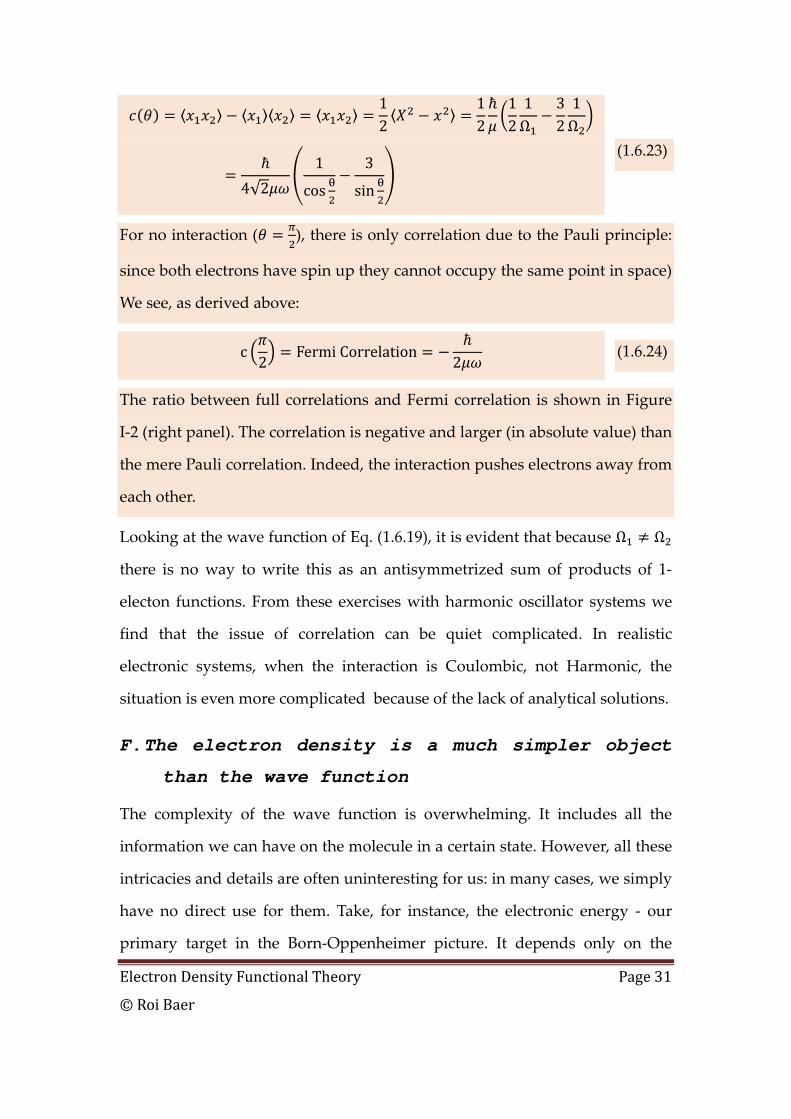
12
12
121Ω
321Ω
4√21
cos
3
sin
(1.6.23)
For no interaction ( ), there is only correlation due to the Pauli principle:
since both electrons have spin up they cannot occupy the same point in space)
We see, as derived above:
c 2 Fermi Correlation 2 (1.6.24)
The ratio between full correlations and Fermi correlation is shown in Figure
I‐2 (right panel). The correlation is negative and larger (in absolute value) than
the mere Pauli correlation. Indeed, the interaction pushes electrons away from
each other.
Looking at the wave function of Eq. (1.6.19), it is evident that because Ω Ω
there is no way to write this as an antisymmetrized sum of products of 1‐
electon functions. From these exercises with harmonic oscillator systems we
find that the issue of correlation can be quiet complicated. In realistic
electronic systems, when the interaction is Coulombic, not Harmonic, the
situation is even more complicated because of the lack of analytical solutions.
F. The electron density is a much simpler object than the wave function
The complexity of the wave function is overwhelming. It includes all the
information we can have on the molecule in a certain state. However, all these
intricacies and details are often uninteresting for us: in many cases, we simply
have no direct use for them. Take, for instance, the electronic energy ‐ our
primary target in the Born‐Oppenheimer picture. It depends only on the
Electron Density Functional Theory Page 32
© Roi Baer
relative distance of pairs of particles. This is because the electron‐electron
Coulomb repulsion is a pair‐wise interaction.
One interesting quantity, besides energy, that can be extracted from the
electronic wave function is the electron density ( )n r . This 3D function tells us
the expectation value of the density of electrons. That is ( ) 3n d rr is the
expectation value of the number of electrons at a small volume 3d r around
point r . Thus, we can write:
| | (1.7.1)
We use the notation:
| , , … , , , … , … (1.7.2)
Here is the operator corresponding to the electron number density. Since
electrons are point particles, and the position operator for the ith electron is
this operator is defined by:
(1.7.3)
We used the definition of a ‐function, according to which:
(1.7.4)
The ʺfunctionʺ is the density of electron at .
Exercise I‐3
Calculate the expectation value of the electron number density and show that:
, , … , , , … , … (1.7.5)
Solution: Plugging (1.7.3) into (1.7.1) gives:
Electron Density Functional Theory Page 33
© Roi Baer
, , … , , , … , …
, , … ,
, , … , …
, , … ,
, , … , …
(1.7.6)
The last step stems from the Pauli principle: all electrons are identical, so we
can replace electron by electron . The sum is now over identical numbers
so it becomes a mere multiplication as in Eq. (1.7.5).
Looking at Eq. (1.7.5), we see that involves integrating out a huge
amount of wave‐function details. It is as if only the data concerning the
density distribution of a single electron remains! This is multiplied by in
Eq. (1.7.5) so accounts for the combined density of all electrons. Indeed,
integrating over the entire space, one obtains from (1.7.5):
(1.7.7)
Expressing the fact that the total number of electrons is .
Exercise I‐4
Calculate the 1D electron density of the triplet ground state from Exercise I‐2.
Solution: If the wavefunction of Eq. (1.6.6) is taken then:
Electron Density Functional Theory Page 34
© Roi Baer
2
(1.7.8)
We choose to ensure that 2:
12
(1.7.9)
Defining the “average frequency”:
1Ω
12
1Ω
1Ω
1√2
cos sinsin (1.7.10)
We find the density of the state in Eq. (1.6.19) is:
Ω Ω
ΩΩ
Ω 1 2 2Ω Ω
(1.7.11)
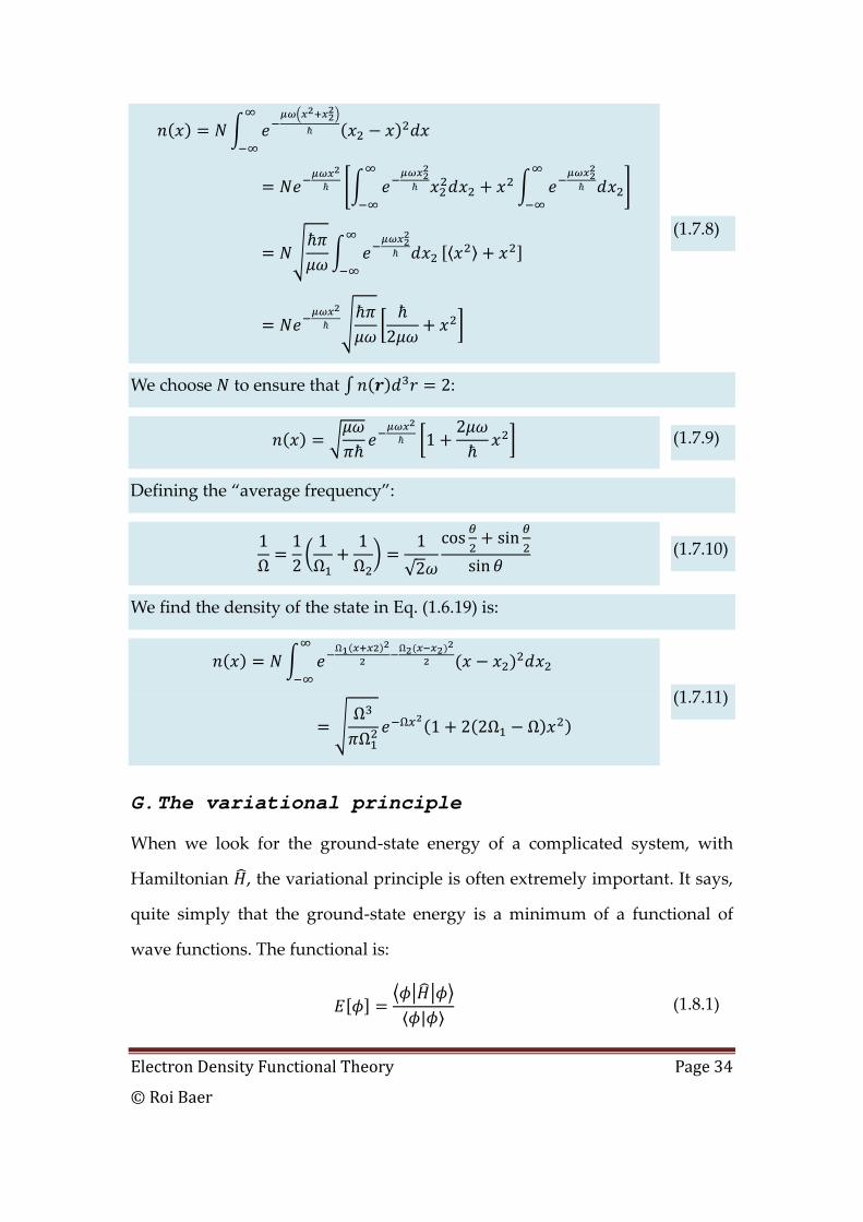
G. The variational principle
When we look for the ground‐state energy of a complicated system, with
Hamiltonian , the variational principle is often extremely important. It says,
quite simply that the ground‐state energy is a minimum of a functional of
wave functions. The functional is:
| (1.8.1)
Electron Density Functional Theory Page 35
© Roi Baer
And the variational principle states that:
(1.8.2)
For all . What this principle allows us is to determine which of the two wave
functions and gives an energy closer to , without knowing .
Simple the one with lower energy is closer.
We can build a parameterized family of functions and determine the
ʺoptimizedʺ parameter as the one that gives minimum to .
Exercise I‐5
Consider the quantum ground‐state problem for a particle in a well
. We consider the family of functions:
√2 (1.8.3)
Here σ is a positive parameter. What is the best function for representing the
ground state?
Solution: The functions are normalized. The energy is . We have:
834 (1.8.4)
Where we used the fact:
2 8 (1.8.5)
Thus the minimum energy is obtained from:
0 4 3 12
/
(1.8.6)
And so:
Electron Density Functional Theory Page 36
© Roi Baer
8/
34 12
/ 316
1 (1.8.7)
H. Dilation relations
Consider the normalized . From it, we can define a family of normalized
wavefunctions:
/ (1.9.1)
We can check that each member is indeed normalized:
| | | | (1.9.2)
This operation of ʺstretchingʺ the argument of a function is called dilation.
Dilation affects functionals. Consider the kinetic energy functional:
12 (1.9.3)
Exercise I‐6
Prove the dilation relation of and :
(1.9.4)
Solution: We show that this is a simple relation:
12
12
12
(1.9.5)
The potential between all particles is called “homogeneous of order ” if:
, … , , … , (1.9.6)
Electron Density Functional Theory Page 37
© Roi Baer
Examples are 2 is for Harmonic potential wells and harmonic interactions
and 1 is for the Coulomb potential wells and Coulombic interactions.
Exercise I‐7
Prove the dilation relation for homogeneous potentials of order :
(1.9.7)
Solution: For such a potential,
, … , , … , …
,… , , … , …
,… , , … , …
.
(1.9.8)
We combine the results from Eqs. (1.9.4) and (1.9.7) and obtain an interesting
property of the total energy for systems with homogeneous interactions:
(1.9.9)
For a molecule, the interaction between the particles (electrons and nuclei) is
the Coulomb potential ; , … , ; , … , which is
homogeneous of order 1 one finds the energy of a molecule obeys:
Coulomb (1.9.10)
i. The concept of the virial in classical mechanics
First, let us define the virial. For a system with coordinate collectively
denoted as the virial in classical mechanics is the time average of
where is the force vector:
1
Electron Density Functional Theory Page 38
© Roi Baer
It can be shown, that for bound systems:[5]
2
For conservative systems the force is a gradient of the potential, .
The viral relates to dilation of the coordinates through:
. (1.9.11)
For homogeneous potentials we have: , thus:
(1.9.12)
In particular, for 1:
(1.9.13)
We will especially be interested in Coulomb systems, where 1, then:
0 1 (1.9.14)
Exercise I‐8
Eq. (1.9.13) is known as Euler’s equation, after its discoverer. In
Thermodynamics it is extremely useful. Thermodynamics stipulates that if
you know the energy of a system , , as a function of its macroscopic
parameters , , then you have complete thermodynamics knowledge. The
first and second laws of thermodynamics state that:
, (1.9.15)
where , and are respectively the temperature, the pressure and the
chemical potentials. A second stipulation is that is a homogeneous function
of order 1.
From this, show that for all thermodynamical systems
1.
Electron Density Functional Theory Page 39
© Roi Baer
2. .
For homogeneous potentials the viral theorem becomes:
2 (1.9.16)
For Coulomb systems 1:
2 (1.9.17)
From which:
2 (1.9.18)
We now show that this relation holds also in quantum mechanics.
ii. The Virial Theorem in quantum mechanics
Now, if is the ground‐state energy then obtains the minimum and
therefore:
0 (1.9.19)
Plugging this into (1.9.10), one obtains:
0 2 (1.9.20)
Since we know that the optimal value of is 1, then (dropping the symbol
and remembering that all following quantities are ground state expectation
value:
2
12
2 1 (1.9.21)
These relations show that the virial theorem (Eq. (1.9.18) holds in quantum
mechanics provided is the full molecular eigenstate. For molecules 1:
and one has:
Electron Density Functional Theory Page 40
© Roi Baer
2 Coulomb
12
(1.9.22)
A subtle issue: all energies and potentials in the above expressions are
absolute. We usually give energy and potentials only to within an additive
constant. However, the fact that the potential is homogenous, it cannot
tolerate addition of a constant ( is homogeneous of order 2 but is
not).
iii. Slater’s theory of the chemical bond using the viral theorem
What happens when is the electronic eigenstate in the Born Oppenheimer
approximation? If we look only at the electronic wave function we do not
expect Eq. (1.9.21) to be valid. Indeed, using ; where
and ; | | (with obvious summation on nuclei and electrons)
(1.9.23)
Upon dilation / and note that is not dilated. Then
we have for the KE and potential:
1212
12
(1.9.24)
And we define:
Electron Density Functional Theory Page 41
© Roi Baer
, , ;
; ,
, ;
, ; ,
(1.9.25)
We have defined , a two quantity. Of course, the physical interaction
potential is , . The reason we defined this way is that we can
now write:
, (1.9.26)
Note that we inserted the subscript to the KE since now it is only the KE of
the electrons.
One still has the variational principle, i.e. / | 0 (Eq. (1.9.19)):
0 2 , , (1.9.27)
Here we used the fact that . Putting in the
solution 1 we find:
0 2 , (1.9.28)
From the Hellmann‐Feynman theorem (see section XXX) ,
. Adding to the electronic energy the nuclear potential energy
∑ gives the BO energy and since the nuclear
energy is homogeneous of order ‐1, we can use Eq. (1.9.14) and:
0 , (1.9.29)
Plugging all this into eq. (1.9.28) we find Slater’s formula[6]:
Electron Density Functional Theory Page 42
© Roi Baer
(1.9.30)
From this, using (where is the total PE of the
molecule we find also:
2 (1.9.31)
We point out an interesting property of Eq. (1.9.30) is that we can obtain
electronic properties such as kinetic energy or potential energy directly
from the potential surface . This will be important for analyzing properties
of DFT quantities. Note that at stationary points on the Born Oppenheimer
PES where =0 the usual virial relation eq. (1.9.21) holds (with neglect of
nuclear kinetic energies).
Slater derived Eq. (1.9.30) in a different manner, not from variational or
dilation considerations. He used it for analyzing the general nature of
chemical bonding of a diatomic molecule. We follow in his footspteps here.
Consider a diatomic molecule. Suppose the BO curve is give as a potential of
the following form, in terms of the inter‐nuclear distance :
(1.9.32)
Where and are positive constants and typically .For example, in the
case the PE curve is given by the Lennard‐Jones potential then 12 and
6. This potential describes long‐range attraction and short‐range
repulsion. It has a minimum at:
(1.9.33)
One then has:
Electron Density Functional Theory Page 43
© Roi Baer
1 1 (1.9.34)
When ∞ we have: . Let us consider what happens to
the KE as the distance is reduced. Clearly it initially descends, however, at
some distance it reaches a minimum, and below this distance it begins to
increase. Since:
1 1 (1.9.35)
We find the minimum kinetic energy is obtained at a distance somewhat
larger than :
11
11 (1.9.36)
For example, for 12, 6 we find: 1.14 . The sum of electronic
and nuclear potential energy is:
2 22 (1.9.37)
At large , actually increases as the atoms approach. The potential
energy does not rise indefinitely. At some inter‐nuclear distance, larger than
the distance at which the BO potential obtains its minimum, it reaches a
maximum and then starts decreasing. We have:
2 2
22
22
(1.9.38)
For the Lennard Jones potential we have: 1.16 . For we find
that the kinetic energy grows sharply as decreases, while the potential
Electron Density Functional Theory Page 44
© Roi Baer
energy decreases. This sharp behavior can be interpreted as a condensation of
the electron cloud around each nuclei as such a condensation causes increase
in kinetic energy and decrease in electronic potential energy . The total BO
energy continues to drop as long as and then starts rising.
As an application of this theory consider the … system where is a
neutral atom and a distant atomic ion (can also be a molecular ion). The
energy at large distance is that of Eq. (1.9.32) with 0 and where
is the polarizability of and 4. This form of the potential surface
results from a simple exercise in electrostatics. Quantum mechanics is needed
only for calculating the value of the polarizability of , . Slater’s analysis
states that:
32
2
(1.9.39)
So the force due to the total potential energy is repulsive while that due to the
KE is attractive. The KE attraction outweighs the PE repulsion by a factor of
three halves. Slater’s analysis shows that the interaction here is fundamentally
different from that of electrostatics, where the force attributed entirely to the
Coulombic attraction.
Another application is to the simplest chemical bond, that of the molecule.
The text‐book analysis of this molecule assumes that the molecular orbital is a
“bonding” linear combination of the two atomic orbitals (LCAO), both having
the 1s shape: , but each centered on its corresponding nucleus.
Quantitatively this picture is very inaccurate. While it does show binding, its
predicted a bond length is almost 1.4 (while the true bond length is 1.06 )
Electron Density Functional Theory Page 45
© Roi Baer
and its estimate of atomization energy is 1.7 eV while the experimental value
is close to 2.7eV. There are no electron correlation effects here, so the only
source of inaccuracy is the limited efficacy of the small basis.
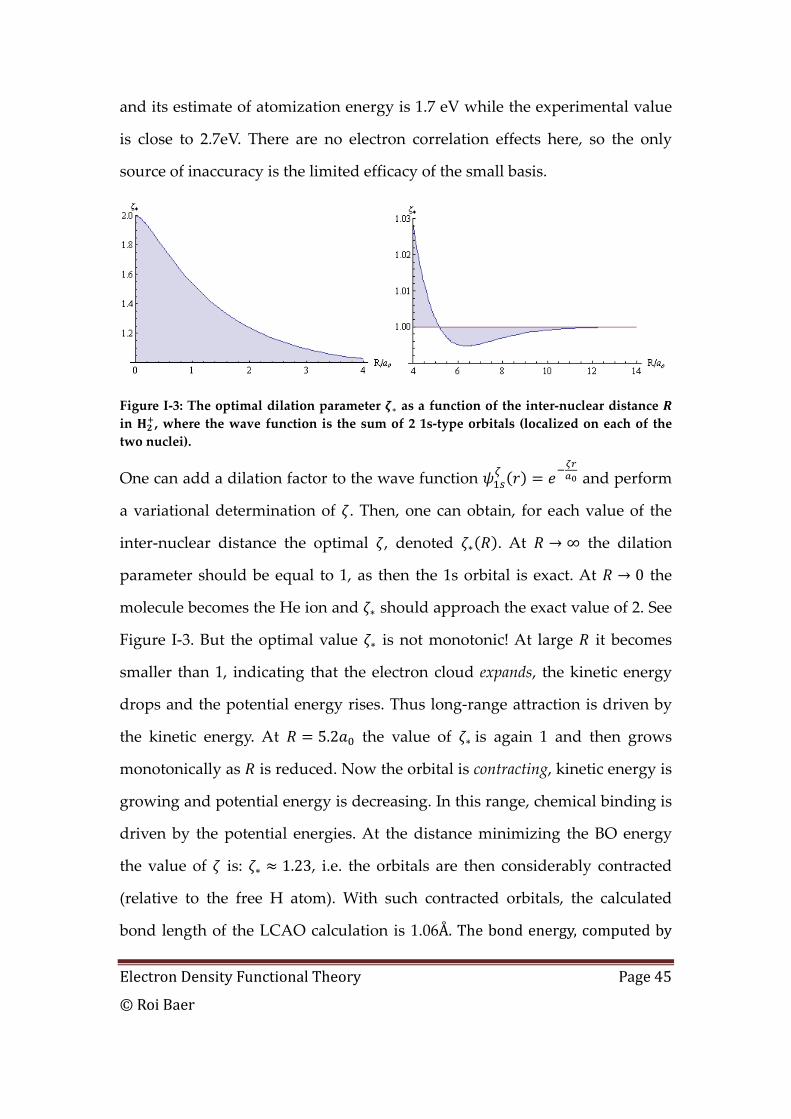
Figure I‐3: The optimal dilation parameter as a function of the inter‐nuclear distance in , where the wave function is the sum of 2 1s‐type orbitals (localized on each of the two nuclei).
One can add a dilation factor to the wave function and perform
a variational determination of . Then, one can obtain, for each value of the
inter‐nuclear distance the optimal , denoted . At ∞ the dilation
parameter should be equal to 1, as then the 1s orbital is exact. At 0 the
molecule becomes the He ion and should approach the exact value of 2. See
Figure I‐3. But the optimal value is not monotonic! At large it becomes
smaller than 1, indicating that the electron cloud expands, the kinetic energy
drops and the potential energy rises. Thus long‐range attraction is driven by
the kinetic energy. At 5.2 the value of is again 1 and then grows
monotonically as is reduced. Now the orbital is contracting, kinetic energy is
growing and potential energy is decreasing. In this range, chemical binding is
driven by the potential energies. At the distance minimizing the BO energy
the value of is: 1.23, i.e. the orbitals are then considerably contracted
(relative to the free H atom). With such contracted orbitals, the calculated
bond length of the LCAO calculation is 1.06 . The bond energy, computed by
Electron Density Functional Theory Page 46
© Roi Baer
subtracting the calculated H2 energy from that of the hydrogen atom gives the
bond energy of 2.35eV. The first to report this type of calculation is in ref [7], a
clear exposition of the calculation is given in refs [8]. These improved
theoretical estimates, with a two‐function basis, achieved with just a single
dilation parameter, show that orbital shapes are crucial for a good description
of chemical bonding.
This result contradicts our intuition regarding the behavior of electrons in a
covalent bond. It seems that a major source of the chemical bond energy in H
is not due to the electrostatic benefit resulting from the placement of electrons
in the middle region separating the two nuclei. Rather, it is due to the
contraction of the electron wave function near each of the nuclei induced by
change in Coulomb potential near that nucleus due to the presence of the
other nuclei. Around one nucleus of H the nuclear Coulombic potential
becomes deeper and distorted towards the second nucleus. As a result, a
contraction of the electron density around the nucleus is obtained, and the
charge placed between the atoms is not in the “midway” region of the bond: it
is between them alright but very close to each nucleus. Each nuclei seems to
share the electron not by placing it midway between them, but rather by
having the electrons much closer to each nucleus.
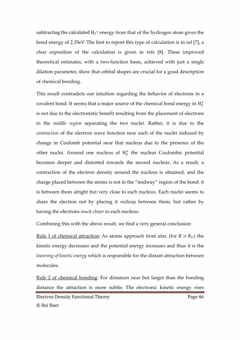
Combining this with the above result, we find a very general conclusion:
Rule 1 of chemical attraction: As atoms approach from afar, (for the
kinetic energy decreases and the potential energy increases and thus it is the
lowering of kinetic energy which is responsible for the distant attraction between
molecules.
Rule 2 of chemical bonding: For distances near but larger than the bonding
distance the attraction is more subtle. The electronic kinetic energy rises
Electron Density Functional Theory Page 47
© Roi Baer
sharply and the potential energy drops even more sharply. Thus, a major
source of energy is the contraction of orbitals around their respective nuclei,
inspired by the deepening of potential wells due to the presence of close‐by
nuclei. The electronic PE is thus the major glue when atoms are close to each
other: It has to offset the nuclear repulsion and the repulsion due to kinetic
energy of electrons.
iv. Other Dilation Facts
Consider the Schrödinger equation:
2 (1.9.40)
We now dilate: we assume is an eigenstate and find the
corresponding Hamiltonian. Note that thus:
2 (1.9.41)
We see that the required Hamiltonian involves a dilated potential and a scalled
mass by a factor .The energy is left intact. Alternatively, we can multiply
through by the square of the dilation factor and obtain:
2 (1.9.42)
Now the potential is dilated and scaled: when then the wave
function is dilated by and the total energy is also scaled by
. This is general for basically any Schrödinger equations and holds for
any number of spatial dimensions.
Now consider homogeneous potentials in 3D: . In this case the
potential transform is indeed a multiplicative scaling: . In
Electron Density Functional Theory Page 48
© Roi Baer
particular, in Coulomb systems, when 1, we find that the potential
scaling is simply by a factor . We can turn around the discussion and state:
If the Coulomb coupling constant is scaled by a factor then the total
energy is scaled by a factor and the wave function is dilated by a
factor . In particular, the density is dilated and scaled as
.
According to the virial theorem, the potential energy and the total energy are
related by , thus the expectation value of the potential and kinetic
energies is scaled by a factor as well.
Exercise I‐9
An application of the above discussion allows an interesting exact conclusion
concerning the ground‐state energy per particle of the homogeneous electron
gas of density (see section XXX for details). Denote this quantity, ,
and the Coulomb coupling constant /4 . Show that:
3 2 (1.9.43)
Hint: Start from , λ λ , . Then take the derivative with
respect to . Then set 1.
I. Introduction to Functionals
i. Definition of a functional and some examples
A formula that accepts a function and maps it to a number is called a
functional. We denote the number a functional maps to a function by
this by the symbol . Take for example the simplest functional: 0.
This functional maps any function to the number zero. A more
interesting functional is:
Electron Density Functional Theory Page 49
© Roi Baer
(1.10.1)
This functional maps to each function its value at a certain point .
Next, consider the functional
1, (1.10.2)
mapping each function its average value in a given volume .
Another familiar example is the kinetic energy functional for a particle of
mass in some wave function :
2 , (1.10.3)
Or the energy for a given potential :
, (1.10.4)
Where:
| | , (1.10.5)
ii. Linear functionals
A functional is called linear if for any two functions and one has:
and if for any
number . The functionals above and are examples of such
functionals, please check. Any linear functional can be written in the form:
. (1.10.6)
The function is called the linear response kernel of . For example, the
linear response kernel of is . And that of is .
Electron Density Functional Theory Page 50
© Roi Baer
iii. Functional Derivatives
Let us now introduce the concept of a ʺfunctional derivativeʺ. Consider the
functional of Eq. (1.10.1). A functional derivative, denoted
measures how changes when we make a small localized change of
at .
Let us give a more detailed definition. Suppose we change the argument
function in by making an arbitrarily small change in Φ .
We use an arbitrary function Φ multiplied by an infinitesimal number
(that is, a number we intend to make vanishingly small at a later statge). In
principle, for any finite the change in has a very complicated
dependence on . But, since is assumed small, we can Taylor expand with
respect to Φ and then “throw out” all terms beyond the term linear in Φ.
This makes sense since we assume that is a small as we want. Thus, the
linear part of is a functional of Φ and it is a linear functional. We denote
the linear response kernel of this functional by the symbol , called “the
functional derivative”. Therefore we can write:
Φ Φ (1.10.7)
Note, that this the linear response kernel is independent of Φ and .
One technique to obtain the kernel is taking Φ . To make
this notion precise, we define:
lim (1.10.8)
Where is a delta function, expressing the fact that we make a
localized change in at r .
Electron Density Functional Theory Page 51
© Roi Baer
Examples
Apply definition (1.10.8) to , and . Find the functional derivatives
and check that Eq. (1.10.7) holds.
Solution:
lim lim
(1.10.9)
The functional derivative comes out , meaning that any
change in made at will not affect , unless it is made at .
Indeed, if we make an arbitrary small change Φ, we have from (1.10.7):
(1.10.10)
And this is seen to be indeed the case directly from the definition of 0
F r in Eq.
(1.10.1).
As for :
lim
lim
(1.10.11)
Another Example
An important functional, we will use is the ʺHartree energyʺ, the classical
repulsion energy associated with a charge distribution :
12 | | (1.10.12)
Electron Density Functional Theory Page 52
© Roi Baer
Prove that the functional derivative of the Hartree Energy, called the Hartree
potential is the electrostatic potential of that density of electrons:
lim| | | |
lim | |
| |
(1.10.13)
Thus, we find as requested that is ineed the electrostatic potential of the
density .
Two shortcuts: when “functional integrating”, one can often use regular
differentiation rules. All one needs to remember is the following shortcuts:
(1.10.14)
And use them within “chain rules”: (where
). An example of the use of this rule is the previous exercise:
(1.10.15)
Another example is the following functional, related to the kinetic energy:
(1.10.16)
The functional derivative is:
Electron Density Functional Theory Page 53
© Roi Baer
2
2 2 (1.10.17)
Here we used the identity: and the shortcut
.
iv. Invertible function functionals and their functional derivatives
Consider a “continuous set of functionals” which is “indexed” by a
continuous variable in some domain . More precisely, assigns a
functional to each in . Let us suppose further that is a function of
defined on the same domain . An example is the relation between the
electrostatic potential and the charge density:
| | (1.10.18)
For any charge distribution the integral forms a the electrostatic
potential . The potential at a give point depends in principle on the
charge density at all points in space. This is a very non‐local dependence.
What about the functional derivative? If one makes a small change in the
function at the point , , how will that affect the functional at ? We
write this as a definition of the functional derivative:
(1.10.19)
In the example above, it is immediately noticeable that:
1| |
(1.10.20)
Electron Density Functional Theory Page 54
© Roi Baer
An interesting concept can arise when one knows in advance that the relation
is unique, i.e.
for all for all (1.10.21)
In this case one can also consider to be a functional of . Indeed:
(1.10.22)
Once can combine this equation with (1.10.20) and see that:
(1.10.23)
This shows that:
(1.10.24)
Thus, there is an inverse relation between the functional derivatives. This is
similar to what happens in usual derivatives with inverse functions. When a
function is invertible we can speak of . The change in due to a
change in is: . Similarly: . Therefore:
.
v. Convex functionals
A function is said to be convex if for any pair of abscisas and the
curve , described by in the interval is always below
the straight line connecting , and , . A more formal
definition is that for any 0 1 we have:
1 1 (1.10.25)
Electron Density Functional Theory Page 55
© Roi Baer
A useful interpretation of the above definition for convexity is in terms of
averages. We can view 1 as a weighted average of the two
points, with positive weights (such an average is usually called a convex
average). In this sense we have convexity obey:
(1.10.26)
This relation is much more general than just 2 points . We can easily show that
for convex functions it holds for any averaging procedure ∑ and
∑ with 0 and ∑ 1. Eq. (1.10.26) is sometimes called
Jensen’s inequality.
One of the important implications of a convex function is that it cannot have a
local minimum: either there is no minimum (for example ) or there
is just one global minimum. If a function is known to be convex and to have a
minimum then any “descent” algorithm is surely to find the (global)
minimum. This is useful.
We can Taylor expand 1 with respect to
, assuming now 1. Then:
1
(1.10.27)
After rearrangement and division by we set to zero and obtain:
(1.10.28)
This relation, if obeyed for all pairs of points, is equivalent to the convexity of
the function. By exchanging and we obtain also:
(1.10.29)
From (1.10.28) we further have, for 0:
Electron Density Functional Theory Page 56
© Roi Baer
12
| |
(1.10.30)
From this, after cancelling and dividing by we find 0 for
arbitrary which means the Hessian is positive definite: another
characteristic of convex functions
A similar definition of convexity can be applied to functionals
1 1 (1.10.31)
And they too have the equivalent differential property, which will be useful
below:
δ (1.10.32)
An example for a convex functional useful for density functional theory is the
so‐called Hartree energy functional:
12 | | (1.10.33)
The second functional derivative of this function is | | which is a
manifestly positive matrix (this is easily seen by Fourier transforming the
function , with result which is positive). Another example is
the von‐Weizsacker kinetic energy functional:
12 (1.10.34)
The physical meaning of this functional is that it gives times the kinetic
energy of a single‐particle with ground state wave function
Electron Density Functional Theory Page 57
© Roi Baer
where . Again, by showing the Hessian is positive definite we
can straightforwardly show this functional is convex First, rewrite it as:
12
18 (1.10.35)
We drop the explicit in the last expression, for brevity. Then, make an
arbitray but small perturbation Φ :
Φ18
ΦΦ (1.10.36)
And expand the denominator to second order in : Φ 1
. Expanding the numerator and performing the multiplication
order by order one can then read off the second order contribution and after
some manipulation bring it to the form:
Φ 8Φ Φ
Φ (1.10.37)
Clearly, this second order term is absolutely non‐negative for all perturbations
and at all physical densities. This shows that the underlying functional
derivative Hessian is positive definite and thus the functional is convex.
A similar condition exists for the second functional derivative. The Jensen
inequality holds here as well:
(1.10.38)
This relation, in combination with the fact that is convex is useful
for developing mean field approaches in Statistical mechanics. It was used by
Gibbs and later, in a quantum context by Peierls.[9]
Electron Density Functional Theory Page 58
© Roi Baer
J. Minimizing functionals is an important part of developing a DFT
Equation Section (Next)Minimization of functions
We start with the problem of minimization of a simple 1D function. Given a
function , we want to find a point such that the function is minimal. It
is clear that the slope of at must be zero. If the slope is positive
then we can go left (decrease ) and reduce . Same logic (but to right) if
it was negative. Thus, a necessary condition for a minimum is:
0 (1.11.1)
Let us expand in a Taylorʹs series the function around the point . Clearly, we
have:
12 (1.11.2)
However, taking Eq. (1.11.1) into account,
12 (1.11.3)
When is extremely close to we may neglect high order terms and then we
see that Eq. (1.11.3) is the equation of a parabola. In order that be a
minimum, we must have an ascent of when we move away from , no
matter which direction we take (left or right). For small displacements ,
we see from Eq. (1.11.3) that the change in is . Since
is always positive, no matter the direction we move, we must
demand that 0 as well. Thus, our necessary conditions for a
minimum are:
0 0 (1.11.4)
Electron Density Functional Theory Page 59
© Roi Baer
Now, let us consider the case of functions of two variables, where
. Notice that we use the ʺtransposeʺ symbol to turn a
column vector into a row vector. Let us Taylor expand around a point :
12
T
T 12
T (1.11.5)
Note that we use the notations:
(1.11.6)
The vector is called the gradient and the matrix the Hessian at .
Note that the Hessian is a symmetric matrix, since the order of differentiation
is immaterial. When is a minimum, moving infinitesimally away from it in
any direction will not change the function. Why? We can show this leads to a
contradiction. Let be an arbitrary direction. If the function decreases when
moving from in that direction, no matter how small the step size, then this
contradicts that is a minimum. Now, if, is an ascent direction, then
will be a descent direction ‐ again a contradiction to being a minimum.
Thus we conclude , that cannot change (to first order) or in other words, the
gradient of at must be zero. Then Eq. (1.11.5) becomes:
12 (1.11.7)
Electron Density Functional Theory Page 60
© Roi Baer
Continuing, in order for this function to have a minimum at the second
term on the right hand side must always be positive. Thus Hessian matrix
must be such that for any vector 0. A matrix having this property
is called ʺpositive definiteʺ (PD). When a PD matrix is symmetric, then its
eigenvalues must be strictly positive. We can summarize the necessary
conditions for a minimum at :
0 . . (1.11.8)
As an example, let us take the function . This function is always
non‐negative, so its minimum is at 0, where it obtains the value 0.
The gradient is indeed zero at , 0,0 :
∂ ,2 , 0
∂ ,2 , 0
(1.11.9)
And the Hessian is 2 where is the 2×2 identity matrix, thus it is trivially
PD.
ii. Constrained minimization: Lagrange multipliers
Next we discuss constrained minimization. Suppose we want to minimize
, , under a constraint that . This is “easy”, since it can be
transformed into an unconstrained minimization. All we have to do is
minimize , . This will give:
, , (1.11.10)
Electron Density Functional Theory Page 61
© Roi Baer
, 2
, ,
,
And we can then search for such that 0 and 0.
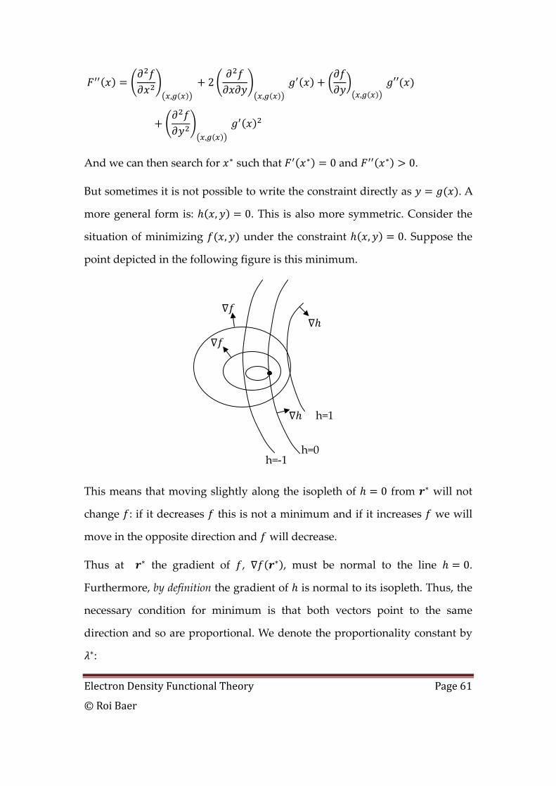
But sometimes it is not possible to write the constraint directly as . A
more general form is: , 0. This is also more symmetric. Consider the
situation of minimizing , under the constraint , 0. Suppose the
point depicted in the following figure is this minimum.
This means that moving slightly along the isopleth of 0 from will not
change : if it decreases this is not a minimum and if it increases we will
move in the opposite direction and will decrease.
Thus at the gradient of , , must be normal to the line 0.
Furthermore, by definition the gradient of is normal to its isopleth. Thus, the
necessary condition for minimum is that both vectors point to the same
direction and so are proportional. We denote the proportionality constant by
:
h=1
h=0h=‐1

Electron Density Functional Theory Page 62
© Roi Baer
0 (1.11.11)
Lagrange noticed that this relation and wrote a Lagrangian for the constrained
problem:
, (1.11.12)
The new variable is called a ʺLagrange multiplierʺ. The necessary conditions
for a minimum in Eq. (1.11.11) translate into the condition of finding a
stationary point of
, 0 (1.11.13)
Where , , , . The derivative with respect to gives us back the
constraint. As an example, consider minimizing , under the
constraint , 1 (i.e. find the point on the unit circle for which
is minimal). We have:
, 1 (1.11.14)
The necessary condition is:
1 2 , 1 2 , 1 0,0,0
12 , 2
12 1
(1.11.15)
The solution is thus:
1√2
1√2 (1.11.16)
Since these are necessary conditions, we need to consider them further (they
might correspond to a maximum). The minimum corresponds only to the
negative solution.

Electron Density Functional Theory Page 63
© Roi Baer
The method of Lagrange multipliers is often more convenient to work with
than direct replacement. The problem is thus that of finding a minimum of
, … , under the constraints , … , , or , … ,
1,… , is:
find such that: for which
for any such that: (1.11.17)
To facilitate such a search, we formulate the Lagrangian function:
, ; (1.11.18)
Our plan is to find the position of which minimes for any choice of and
then change until . At we have assuming a minimum at a point
. A necessary condition for the constrained minimum to be achieved at the
point and with the Lagrange multipliers is:
, ; 0
, ; 0 (1.11.19)
Note that is not necessarily a minimizer of . In fact the opposite is tue:
is a maximizer of and the search for constrained minimizations is a search
for saddle points (see ref. [10] for a method to solve such a problem on the
large scale).
It is interesting now to ask how changes if we change the value of the
constraint . Indeed, when the constraints are changed, the optimized point
and Lagrange multiplier can change, so the Lagrangian is changed:
, ; , ; , ; (1.11.20)
Now, because of Eq. (1.11.19) we find:

Electron Density Functional Theory Page 64
© Roi Baer
, ; , ; , ;
, ; , ; (1.11.21)
Thus:
, ; , ; (1.11.22)
Since , ; ; we find:
; ; (1.11.23)
This equation reveals the “meaning” of the Lagrange multipliers at the
optimal point: they are equal to the rate at which the optimal value of the
minimized function changes when , the value of the constraint, is
changed. This is an important result which we use below whenever we want
to give physical significance to Lagrange multipliers.
iii. Minimization of functionals
The same considerations for functions apply for functionals. Given a
functional ( )I f , a necessary condition for its minimum is:
0 (1.11.24)
For example, consider a 1D classical particle of mass m in a potential well
. The action is a functional of the trajectory of this particle:
12 (1.11.25)
For any trajectory between times and , returns a number.
Lagrange showed that finding the trajectory that makes stationary
Electron Density Functional Theory Page 65
© Roi Baer
(although, not necessarily minimal), under the condition that and
are given and thus not varied, is equivalent to solving Newtonʹs
equations under these same constraints. The functional differentiation of the
kinetic energy is performed with:
2 2
2 2 (1.11.26)
The condition for stationarity of the action under changes in the trajectory
which leave the edges intact give:
0 (1.11.27)
From which we obtain Newtonʹs equation . This equation
must be solved subject to the given constraints at the endpoints, i.e.
and .
Minimizing functionals with constraints can again be done using Lagrange
multipliers. Then one defines:
, (1.11.28)
And the necessary conditions are:
,0
,0 (1.11.29)
For example, let us solve the following problem. Find the shape in a plane of a
closed contour encircling maximal area under the constraint of a given
circumference . We need to find the contour given by with 2
which gives zero variation to
Electron Density Functional Theory Page 66
© Roi Baer
, (1.11.30)
Where is the area and is the circumference. We limit ourselves to curves
that can be uniquely defined. A point on the curve, is defined by the angle
and the distance from the origin . The vector to a point on the curve and
its derivatibe is:
cos , sin
cos , sin sin , cos . (1.11.31)
The area of a small arc from to is | |
| | . Notice that | | and so .
The square circumference is: . Thus
| | . Thus, the area is a functional is:
12
(1.11.32)
The functional derivative of S is easy:
(1.11.33)
The functional derivative of is computed by adding a “small” function :
( ) ( )2 2 2
02
2 2
0
22 2
2 20
2 2
2 21
l r r d l
r r r r d l
r rr r d l
r r
π
π
π
δ ε ε θ
ε ε θ
ε εθ
′ ′ ′= + + + −
′ ′ ′ ′= + + + −
′ ′+′ ′= + + −′+
∫∫
∫
(1.11.34)
Then, we can use ( )211 1
2Oη η η+ = + + so:

Electron Density Functional Theory Page 67
© Roi Baer
2
2 20
r rl d
r r
π ε εδ θ
′ ′+ ′=′+
∫ (1.11.35)
Integrating by parts the second term (remembering that the end terms drop
because 2 is the same point as 0:
√ √ (1.11.36)
We thus get:
√ √ (1.11.37)
We define the Lagrangian:
(1.11.38)
And get the maximum from:
0√ √
(1.11.39)
Clearly, a solution is , a constant, since then all derivatives are zero.
The curve is then circle of radius and given the circumference, we have:
/2 .
EXERCISES FOR CHAPTER 1
1) Consider a system of two particles in a harmonic well. Each particle repels the other.
The potential energy is , . We assume that
the system is bound (so 0 2 ). (a) Write down the exact Hamiltonian for this system, assuming the mass are and . (b) Make a transformation separating the Hamiltonian into two uncoupled particles: the center of mass
and the reduced mass . Write the Hamiltonian of each part and determine the mass of each particle. What are the masses when ? (c) Write down the energy levels of the system and the eigenfunctions. (d) Now make a Born‐Oppenheimer approximation. Assuming , determine the Born
Electron Density Functional Theory Page 68
© Roi Baer
Oppenheimer potential surface (obtained when is considered a parameter). Solution: The Hamiltonian is:
2 212
12
12
.
In the new coordinates:
, , , . If , is any function than we can define the “same” scalar function as
, , .
2) Calculate the correlation in the case of a singlet, where both electrons are in the ground state orbital and when one is in the ground state orbital and the other in the first excited orbital.
II. My first density functional: Thomas-Fermi Theory
A. Basic concepts in the electron gas and the
Thomas-Fermi Theory
Thomas and Fermi assumed that the energy of an atom or a molecule can be
written as a functional of the 1‐particle density as follows:
12 | | (2.1.1)
(Note, for use via the Born‐Oppenheimer approximation, to this energy we
need to add the nuclear‐nuclear repulsion energy.) They then assumed that
the density that characterizes the ground‐state minimizes this functional
under the constraint:
(2.1.2)
The first question, beyond the rigor of this approach is, what is the kinetic
energy functional? In order to take into account the Fermi nature and the

Electron Density Functional Theory Page 69
© Roi Baer
quantum nature of the electrons, this functional must include both these
considerations. The Thomas Fermi solution is to assume:
(2.1.3)
What shall we take for ? Consider first a simple case: a homogeneous gas
of density (i.e. is independent of ). Furthermore, let us assume that the
electrons are non‐interacting. This is a simple enough system to enable the
analytic calculation of the kinetic energy functional. From the form of (2.1.3)
we see that the total kinetic energy is the sum of contributions of various
infinitesimal cells in space. Each cell contains electrons and so, if we
interpret as the kinetic energy per electron of a homogeneous gas of non‐
interacting electrons then this sum is yields exactly the total kinetic energy for
this homogeneous gas. The Thomas‐Fermi approximation then uses this same
also for the inhomogeneous interacting case.
Let us now compute . Consider a homogeneous gas of N uncharged electrons.
They are non‐interacting. These electrons are put in a cubic cell of length . The
electron density is everywhere the same .
We assume the wave functions are periodic in the box. According to Fourier’s
theorem, we can write any periodic wave function as a linear combination of
plane‐waves, as follows:
√ (2.1.4)
Where:
, , . (2.1.5)
Electron Density Functional Theory Page 70
© Roi Baer
and / / are integers. Fourier’s theorem is based on the orthonormality of
the plane waves
|1
, (2.1.6)
Where we defined
√2
(2.1.7)
We imagine 3‐dimensional k‐space divided into an array of small
compartments, indexed by a set of integers , , or by the vector .
Each compartment is of k‐length Δ and its k‐volume is Δ . For
large r‐space boxes the k‐space compartment is extremely small since Δ is
proportional to the inverse box volume. Since we are interested eventually in
the limit ∞, we may assume approximate sums of any function over
the discrete values of by integrals:
2 V ∞ (2.1.8)
Let’s show that plane‐waves are eigenstates of kinetic energy operator :
1√ 2 (2.1.9)
Now, consider the wavefunction of the non‐interacting electrons in their
ground‐state. Since they are non‐interacting, this wave‐function is a product
of single‐electron wave‐functions:
Ψ / / (2.1.10)
Here is the state of a spin‐up electron with wave vector k. while is
the state of a spin down electron with wave vector k. Anticipating the
Electron Density Functional Theory Page 71
© Roi Baer
antisymmetry, we build this wave function by placing 2 electrons in the same
spatial orbital (once with spin up and the other with spin down). Since non‐
interacting electrons have only one type of energy, i.e. kinetic energy:
∑ , we can easily show that (2.1.10) is an eigenstate of the
Hamiltonian:
Ψ 2 / /
2k
2
/
/ /
2k
2
/Ψ
(2.1.11)
One sees that the energy is just the sum of kinetic energy ∑ 2/ in each
spin‐orbital of the product wave function. Let us now antisymmetrized this
product wave function. We do this by adding all products resulting from even
permutations of the electrons and subtracting all odd permutation products.
One convenient way to represent such a sum is using a determinant, called a
Slater wave function:
Ψ1√ !
det . (2.1.12)
For this wave function to be minimal energy must fill 2 electrons per level
starting from the lowest kinetic energy and going up until electrons are
exhausted. Denote the highest filled level by . Then:
2 . (2.1.13)
Electron Density Functional Theory Page 72
© Roi Baer
Where is 0 if is negative and 1 otherwise. This is called the Heaviside
function. We now perform the integral using spherical coordinates:
2 4 243 2 3 .
(2.1.14)
The number of filled orbitals is the product of the real‐sapce volum and the
k‐space occupied state volume, divided by 2 . Since 2 and the
density is we have:
23 . (2.1.15)
The electron density determined directly the highest filled momentum state:
2V2π 2 4
2V2π 4 2 5
22 2 5 .
(2.1.16)
The energy per particle is:
12 5
35 2
35 2 3 / , (2.1.17)
where:
35 2 3π
310 3π au 2.871 au . (2.1.18)
Plugging into Eq. (2.1.3), the Thomas‐Fermi kinetic energy functional is
obtained to be used in Eq. (2.1.1):
. (2.1.19)
============================================
Exercise: The Thomas Fermi functional for the hydrogen atom.
a. Repeat the calculation above but now for a “spin‐polarized HEG”. That is, do not assume that there are 2 electrons in each k‐state (the “spin‐unpolarized” case) but instead, that all spins are up and so there is only one electron per k‐state.
Electron Density Functional Theory Page 73
© Roi Baer
b. Since the electron in a hydrogen‐like atom is spin‐polarized, use the Thomas‐Fermi KE functional derived in (a) and compare its estimation of the kinetic energy of the electron in a hydrogen‐like atom to the exact value. Using the exact kinetic energy in the hydrogen atom (you can find it using the virial theorem), assess the quality of the result as a function of the nucleus charge Z.
============================================
B. Minimization of the Thomas-Fermi energy
Now, according to the TF theory, the true ground‐state electron density is the
one that minimizes . But the electron density must also account for the
required number of electrons of , so there is a constraint for the
minimization:
(2.1.20)
Thus, we must build a Lagrangian to be minimized as:
, (2.1.21)
Minimizing it gives the Thomas‐Fermi equation:
0 (2.1.22)
We see that the Lagrange constant is the chemical potential, since it is equal
to the change in energy when we perturb the density and this change is
everywhere constant. We must now compute the functional derivatives:
/ 53
/
12 | | | |
(2.1.23)
Plugging into Eq.(2.1.22), one obtains the Thomas‐Fermi equation for an atom:

Electron Density Functional Theory Page 74
© Roi Baer
53
/| | (2.1.24)
This is an integral equation for . It is called the integral Thomas‐Fermi
equation. The potential is due to the positive charge, hence we can write:
| | . Now we can define a total potential
| | , (2.1.25)
as the sum of the total electrostatic potential and the chemical potential. Since
4 , we have:
4 , (2.1.26)
leading to an equation for the total potential:
14
35
/
(2.1.27)
This is called the ʺdifferential Thomas Fermi equationʺ. The constant is
buried in but it did not disappear: it must be chosen so that Eq. (2.1.20) is
obeyed. Furthermore, it is clear that the potential is manifestly non‐
negative in TF theory (otherwise we could not take its square root).
As we showed (see Eq. (1.11.23)), can be shown to act as a chemical
potential, i.e. –. We will not solve this equation for atoms or
molecules. We just comment that it gives a smoothed value for the atomic
density, not showing the shell structure. We can see this in the following
figure, where we plot the radial density as computed by a relatively accurate
theory, such as Hartree‐Fock and the TFD (Thomas‐Fermi‐Dirac) theory.
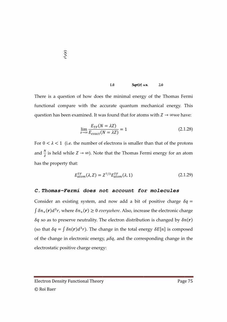
Elec
© R
The
fun
que
For
and
has
C.
Con
(so
of t
elec
ctron Dens
Roi Baer
ere is a qu
nctional co
estion has b
r 0 1
d is held
s the prope
Thomas-
nsider an
, w
so as to pr
that
the change
ctrostatic p
ity Functio
uestion of
ompare w
been exam
l
1 (i.e. the n
while
erty that:
-Fermi
existing s
where
reserve neu
e in electro
positive cha
onal Theory
how does
ith the ac
mined. It wa
im
number of
∞). Note
,
does no
system, an
0 ev
utrality. Th
. The ch
onic energy
arge energ
y
s the minim
ccurate qu
as found th
electrons
e that the T
/
ot acco
nd now ad
verywhere. A
he electron
hange in th
y, , and
gy:
mal energ
uantum m
hat for atom
1
is smaller
Thomas Fe
, 1
ount fo
dd a bit o
Also, incre
n distributi
he total ene
d the corre
gy of the T
mechanical
ms with
than that
ermi energ
or molec
of positive
ase the ele
ion is chan
ergy
esponding
Pag
Thomas Fe
energy. T
∞we ha
(2.1
of the prot
gy for an a
(2.1
cules
e charge
ctronic cha
nged by
is compo
change in
e 75
ermi
This
ave:
1.28)
tons
atom
1.29)
arge
osed
n the
Electron Density Functional Theory Page 76
© Roi Baer
| | (2.1.30)
Using the definition of the total potential in Eq. (2.1.25) we find:
(2.1.31)
Since everywhere we add positive charge, i.e. 0 and since is non‐
negative everywhere, this process increases the total energy! In TF theory
addition of infinitesimal positive charge followed by addition of a
compensating electronic charge causes an increase in total energy of the
system. In a more elaborate treatment Teller showed[11] that the total energy
of any diatomic molecule is higher than the sum of energy of its constituent
atoms, i.e. that TF theory cannot account for stable molecules! He concluded
that Thomas Fermi theory is not very useful for chemistry.
D. Thomas-Fermi Screening
When a point impurity is inserted into an electronic system, it pulls (Z
positive) or repels ( negative) electrons towards it. This has an effect that the
impurity is partially screened by opposite charge and so it has a smaller effect
on distant charges. Let us study this phenomenon in the electron gas, using
Thomas‐Fermi theory. The homogeneous gas of electrons is a model for ideal
metals, so the screening effect we address here is relevant for many metallic
systems. Macroscopically, the “free” metal electrons completely screen the
charged impurity. However microscopically, perfect screening is not possible
because electrons have kinetic energy – even at zero temperature – and a short
ranged electric field develops around the impurity. Thomas Fermi theory
Electron Density Functional Theory Page 77
© Roi Baer
takes kinetic energy effects into account and can be used to estimate the form
of the local electric field, specifically its size or length scale.
Let us study an unperturbed homogeneous electron gas using Thomas‐Fermi
theory. Such a “gas” has no structure and it is characterized by only one
parameter: its density . In order to neutralize it and support the electron
homogeneity, we add positive smeared homogeneous charge density .
All the Coulomb energies (e‐e, e‐N and N‐N) cancel exactly so the only energy
left is the electronic kinetic energy:
/ (2.2.1)
The constraint minimization of this functional yields the following condition,
relating the density to the chemical potential:
53
/ (2.2.2)
Comparing with Eq. (2.1.15), and using Eq. (2.1.18) we find for the chemical
potential:
53 3
/
2 (2.2.3)
Thus we see that indeed the electron density is constant and the chemical
potential is equal to the kinetic energy corresponding to the maximal
occupied momentum .
Now we introduce a positive charge . The density of electrons is changed:
(2.2.4)
It is physically clear that is localized around the impurity (assumed at
the origin). We therefore have for the total energy of the system in terms of :

Electron Density Functional Theory Page 78
© Roi Baer
/
2 | | (2.2.5)
The corresponding TF equation comes from minimizing:
53
/
| | (2.2.6)
We write: | | and so:
53
/ (2.2.7)
Upon linearizing, assuming :
53
/ 123 (2.2.8)
We can write: / and so:
109
/ (2.2.9)
Finally since 4 we have:
109 4
/ (2.2.10)
We have from Eq. (2.1.15) 3 and we use the definition of the
Bohr radius , defining the Thomas Fermi screening parameter :
109 4
/
41 (2.2.11)
With this we have the equation:
(2.2.12)

Electron Density Functional Theory Page 79
© Roi Baer
Passing to spherical coordinates we find:
1Δ . (2.2.13)
Defining we find:
Δ (2.2.14)
The homogeneous equation is which has the solution
. Clearly, for a localized potential solution we must take
0. To this we need add any solution of the inhomogeneous equation
which clearly is Δ . Thus:
Δ (2.2.15)
This leads to:
Δ (2.2.16)
In the limit that 0 we must have 0 since the electronic charge
has no cusps. Thus . The total electrostatic potential is
Δ (2.2.17)
Aside from the constant Δ , far from the impurity the surface integral of
evaluates to zero and by Gauss’s theorem a large sphere around the impurity
includes zero charge in it, meaning that the total amount of electronic charge
pulled into the sphere is exactly equal to that of the impurity ( ).
It is interesting that the screening length is proportional to / or to / .
The higher the density the smaller the length, i.e. the more efficient is the
screening, however, the dependence on is mild because of the small
exponent. It is also interesting to note that is independent of . However,
this latter results holds only in so far as our linearization is valid. For strong
Electron Density Functional Theory Page 80
© Roi Baer
impurities the non‐linear equation will give a different result and the
screening will depend on .
E. Von Weizsäcker kinetic energy
The Thomas Fermi kinetic energy density functional is exact in the limit of
non‐interacting homogeneous gas of electrons in an infinite box. We would
like to mention here another density functional which is exact in a certain
limit, i.e the limit of a single electron. In this case the kinetic energy is:
. For wave functions that decay to zero at
∞, one can integrate by parts and obtain , stressing the
absolute positivity of kinetic energy (it cannot be zero). Finally, if is a
non‐degenerate ground‐state it can be written as and so we
obtain the kinetic energy functional of von Weizsäcker:
2 (2.2.18)
Which can be written as follows, using local wave vector:
12 (2.2.19)
So:
2 (2.2.20)
This functional is now used for any density, even a many electron one. The
variation is:
8ΦΦ (2.2.21)

Electron Density Functional Theory Page 81
© Roi Baer
Working this out to linear terms in , using: Φ 1
Φ we obtain:
82 Φ Φ
(2.2.22)
Which after integration by parts of the first term finally gives:
8 2 Φ (2.2.23)
Thus the von‐Weizsäcker potential is:
8 2 (2.2.24)
Which can be written more compactly as:
2 (2.2.25)
Exercise: For 1‐electron system, discuss the claims: 1) The wave vector is
the gradient of the log of the of the wavefunction: log (2) the
von Weizsäcker potential is the potential for which is the ground state
density.
III. Many-electron wave functions
A. The electron spin
Zeeman has shown that a small magnetic field causes the splitting of energy
levels in atoms. Each atomic level is split into a doublet. The amount of
splitting is proportional to the field. At zero field these doublets are
degenerate. The conclusion is that the electron has an intrinsic magnetic
moment which can take two values. The states of the internal magnetic
Electron Density Functional Theory Page 82
© Roi Baer
moment of the electron are assumed to be proportional to an internal angular
momentum called “spin”. The spin of an electron can is assumed to have two
values . This is an additional “degree of freedom”. It is not continuous, but
is nevertheless it is degree of freedom. We denote a spin‐orbital
, where is a point in 3D space and is a “spin variable”, which allows
us to perform a inner product of spin as explained now. There are two
possible spin functions for an electron, denotes spin up and spin
down. These two states are complete and orthonormal:
| 1
| 0
| 0
| 1
The variable is just a mneumonic. With new notation, we have:
| , , (3.1.1)
B. The Pauli principle
The electronic wavefunctions are functions of electronic coordinates and
spins , … , . Here , . The Pauli principle states that this
wavefunction must be antisymmetric with respect to interchange of two
electrons:
… ,… , , … … ,… , , … (3.2.1)
Electron Density Functional Theory Page 83
© Roi Baer
This is a “boundary condition” we impose while solving for any electronic
wave function.
C. The Excited states of the Helium atom
How should we represent the, in an approximate form, the low lying excited
states of the Helium atom. He+ has two low lying orbitals 1s and 2s (the 2p
orbitals are degenerate with the 2s, but we will not consider them because in
the Helium atom they are of much higher energy. We can form a 2‐electron
wavefunction by: , .
The excited states will involve excitation of an electron to the 2s orbital. We
can then write:
,
,
,
,
(3.3.1)
The first 3 states form a triplet the total spin is 1. The last is again a singlet
(like the ground state).
D. The Slater wave function is the basic anti-
symmetric function describing N electrons in
N orbitals
The previous example is difficult to generalize. In order to develop a way to
easily represent antisymmetric functions of all types, we consider the
following 2‐electron function, composed of 2 1‐electron spin‐orbitals:
Electron Density Functional Theory Page 84
© Roi Baer
Ψ ,1√2
1√2
(3.4.1)
If we choose the orbitals to be orthonormal, then:
Ψ|Ψ Ψ , Ψ ,12122 1
(3.4.2)
E. Without loss of generality, we may assume the orbitals of a Slater wave function are
orthogonal
But what happens if the orbitals are not orthogonal? Suppose that the orbitals
were not orthonormal:
(3.5.1)
It is then possible to “orthonormalize” them. i.e define two linear
combinations which are orthonormal. Define:
(3.5.2)
and demand: . Then:
,
(3.5.3)
Thus: or . Note also that det det / .There are
many solutions to this equation. (For example, if is a solution then so is
where is any unitary matrix.) Each solution will give us a different set
Electron Density Functional Theory Page 85
© Roi Baer
of orthonormal orbitals. The Slater wave function made out from these new
orbitals is:
det det det det
1√det
det (3.5.4)
Thus, the new wavefunction is the same as the old one, up to multiplication
by constant! Yet, it is always more convenient to work with normalized
orbitals, so we can assume the orbitals are orthonormal without any loss of
generality. This development also shows that given any set of N orbitals from
which the Slater wave function has been constructed, we can take N linear
combinations of the orbitals to obtain new orbitals that give the same Slater
wave function up to a constant factor.
F. Any antisymmetric function can be expanded as a sum of basic Slater (determinantal) functions
For orthonormal orbitals, the normalization is easy to compute. We write
explicitly the determinant as:
det … ,… , …
…
(3.6.1)
Where . . is a permutation of the numbers 1… (there are ! such
permutations). Each permutation can be obtained from a series of pair
swapping operations. For example: 132 is obtained from 123 by switching
the pair of numbers in position 2 and 3. We write this as: 132 123 .
2413 is obtained from 1234 by three operations:
1234 2134 2143 2413 (3.6.2)
Electron Density Functional Theory Page 86
© Roi Baer
If the number of switches is odd the permutation is odd and … 1; if the
number of switches is even, the permutation is even and … 0. The
normalization of a determinantal wave function composed of orthonormal
orbitals is:
|det … ,… , | …
… … …… …
… …
… …
(3.6.3)
Because of orthonormality the orbital integral is zero unless k ki j= .
These integrals appear in products so the product is non‐zero only if k ki j=
for all 1… . The only conclusion is, that the two permutations must be
identical and:
|det … ,… , | … 1… …
! (3.6.4)
We conclude that the normalization factor of a determinantal wave function of
orthonormal orbitals is √ ! and write:
1√ !
det … | … (3.6.5)
Given a set of orthonormal single‐electron spin‐orbitals
, 1,2, … , , we can consider the space of all linear combinations of
all ‐particle determinants that can be made. There are !! !
ways
to select determinants so this is the dimension of the space. The dimension
grows factorially with . A typical antisymmetric wave function can e
approached by linear combinations of these determinants:
Electron Density Functional Theory Page 87
© Roi Baer
Ψ ,… ,1√ ! ,…,
,…,
det … (3.6.6)
The sum is over all selections of integers, where each selection is ordered so
that . If the orbitals are orthogonal, the constants ,…, are
obtained from:
,…,1√ !
det … Ψ ,… , … (3.6.7)
G. Determinant expectation values
In this section we discuss the calculation of expectation values of many‐
electron operators for electrons within a given Slater wave function
Ψ ,… ,√ !
det … . We assume the orbitals are
orthonormal: .
i. One-body operators
Consider an operator which operates on an electron with spin‐
coordinates . For electrons we define the sum of for each electron
N
, (3.6.8)
Examples: when electrons are in a potential well , the total potential
energy operator is ∑ ; the total kinetic energy is:
∑ ∑ .
When the system of electrons is in a given Slater wave function
Ψ ,… ,√ !
det … , then using the notation of (3.6.3),
we have:
Electron Density Functional Theory Page 88
© Roi Baer
Ψ Ψ
1! det … det … …
1!
| |……
(3.6.9)
Once again, a massive cancellation of terms happens in the first integral.
Inspection shows that both permutations, and , must be equal otherwise
there is always an orbital integral for which the integrals is zero.
When the permutations are identical we have:
Ψ Ψ1!
| |…
| | (3.6.10)
As an example, let us take the electron density ∑ . Thus:
| , | (3.6.11)
Conclusion: The matrix element of a 1‐particle operator is the sum of its
single‐electron matrix elements.
ii. Two-body operators
Consider an operator , which operates on two electrons with spin‐
coordinates and . For electrons we define the sum of on all pairs of
electrons
,N
12 ,
N
, (3.6.12)
Examples: The 2‐electron interaction potential is , | |. The total
interaction energy operator is: ∑ ∑ , .

Electron Density Functional Theory Page 89
© Roi Baer
We compute the expectation value
Ψ Ψ
1! det … det … …
1!12 | |
……
,
(3.6.13)
Where we used the notation:
| | , (3.6.14)
The following symmetry properties hold from the above definition:
| | | | | |
| | (3.6.15)
For a pair of permutations to contribute to the integral in Eq. (3.6.13), the
permutations must either be identical or involve the permutation of a single
pair of orbitals. Thus:
Ψ Ψ12 | | | |
, (3.6.16)
IV. The Hartree-Fock Theory
A. The Hartree-Fock Energy and Equations
The variational principle says that the lowest expectation value of the
electronic Hamiltonian attained by the ground‐state. This Hamiltonian, in the
non‐relativistic approximation, for electrons is given by:
Electron Density Functional Theory Page 90
© Roi Baer
21 (4.1.1)
Where the “one body” operator is
2 (4.1.2)
And the two‐body Coulomb repulsion operator is:
21
| | (4.1.3)
Given a family of wave functions we can choose the “best” of them by finding
that which minimizes the expectation value of . For the Slater wave
functions Ψ | … |, the energy to be minimized is:
Ψ | |Ψ … (4.1.4)
Because we want the orbitals to be orthonormal, we write a Lagrangian:
… …,
(4.1.5)
The minimum is attained by:
0… …
(4.1.6)
Let us try a solution with
12 (4.1.7)
i.e.:
… (4.1.8)
Electron Density Functional Theory Page 91
© Roi Baer
If we can solve this equation, and if the solutions are naturally orthogonal,
then we have obtained the necessary conditions for a minimum. Now, we
only need to estimate the left hand side of this equation. From the previous
work, we know:
HF … ΨS ΨS ΨS ΨS (4.1.9)
where
ΨS ΨS … (4.1.10)
Is the “one body energy” defined the as the sum of kinetic energy and
ʺexternalʺ energy (i.e. energy due to the frozen nuclei):
2 (4.1.11)
Furthermore, the 2‐electron energy can be written as:
ΨS ΨS 21 1
,
… …
(4.1.12)
Where the direct or Hartree energy is:
… 21
,
, (4.1.13)
and the energy exchange is
… 21
,
. (4.1.14)
Electron Density Functional Theory Page 92
© Roi Baer
The direct energy is numerically equal to the Hartree energy which is a
functional of the Slater wave function electron density Ψ | |Ψ
∑ | , | :
2 | | (4.1.15)
The exchange energy is numerically equal to the “exchange energy”
which is a functional of the density matrix defined by
, (4.1.16)
As:
2| , || | (4.1.17)
Notice that: , . The density matrix is idempotent:
, , , (4.1.18)
This result shows that the DM is a projection operator, projecting onto the
space of orbitals which defines the Slater wave function.
With the direct and exchange energies we also define their functional
derivatives:
Electron Density Functional Theory Page 93
© Roi Baer
12
,
2 | |,
2 2 | |,
2 | |
2 | | 2
2
(4.1.19)
Where in the last line we defined the Hartree potential:
| || | | | (4.1.20)
Then the direct energy can also be written as a functional of the orbitals:
…12 | |
12
12 Ψ Ψ (4.1.21)
where ∑ is the total Hartree potential. A similar treatment
exists for the exchange energy functional derivative:
21
,
2 2 | |,
2 | |
2 | | 2
(4.1.22)
Electron Density Functional Theory Page 94
© Roi Baer
Where the last equality is based on a definition of a one‐particle exchange
operator:
| |
,| |
(4.1.23)
Then the exchange energy is written as a functional of the orbitals:
…12
12 Ψ Ψ (4.1.24)
where ∑ is the total exchange operator. The other functional
derivatives needed are:
2 (4.1.25)
and
2 (4.1.26)
Thus:
2 (4.1.27)
Plugging all these terms into Eq. (4.1.7), we obtain the Hartree‐Fock
equations:
(4.1.28)
where:
(4.1.29)
Electron Density Functional Theory Page 95
© Roi Baer
Equations (4.1.28) seem very much like 1‐electron eigenvalue equations of the
Schrödinger equation, except that instead of a regular Hamiltonian, we have a
Fock operator including the non‐local exchange. We showed in the exercise
that is Hermitean and thus so is , i.e. . We can thus
choose the orbital solutions of the eigenvalue equation (4.1.28) orthonormal.
This shows that the choice Eq. (4.1.7) is indeed acceptable.
Because and themselves depend on , the Hartree‐Fock equations
are fundamentally different from the Schrödinger Equation: they are nonlinear
equations.
Now that the sum of orbital energies is:
| | | | | |
, … , 2 , … , 2 , … ,
(4.1.30)
This shows that the orbital sum is not equal to the energy of the wave
function, since it involves double counting of the direct and exchange
energies. The HF energy is thus:
, … , , … , , … , (4.1.31)
B. Restricted closed-shell Hartree-Fock
For molecules with even number of electrons in a spin‐singlet state, we can
impose the following structure on the Slater wave function. We can assume
that the 2 spin‐orbitals come in pairs: and
. Thus each orbital , 1,… , /2 is “doubly occupied” by
electrons of both spins. By imposing this constraint we obtain the “restricted”
Hartree‐Fock ground state. It will sometime be of higher energy than the fully
Electron Density Functional Theory Page 96
© Roi Baer
unrestricted case. However, the wave function has a well‐defined spin which
may be advantageous in some applications.
The Restricted Hartree‐Fock (RHF) energy in the closed shell case remain
essentially the same except for counting business. We can formulate all
expressions using only the spatial orbitals. Indeed, the RHF energy is given
by:
, … , /
2/
4 , … , / 2 , … , / (4.2.1)
Where , … , / and , … , / are the orbital functionals defined in
Eqs. (4.1.13) and (4.1.14) respectively. The reason for multiplying the one
body part by two is evident: each orbitals is double occupied so has double
contribution. The direct part is multiplied by 4 since the density is multiplied
by two and the direct part depends on the density multiplied by itself. Finally,
the exchange part is multiplied by 2 and not 4 since only and
contribute, while and do not (so only half the contribution of
direct).
The RHF equations are then:
2 (4.2.2)
Where:
2| || |
/
(4.2.3)
and
Electron Density Functional Theory Page 97
© Roi Baer
| |
/
(4.2.4)
Note that the Hartree interaction is between each electron and all other
electrons regardless of their spin while the exchange interaction involves each
electrons with all other electrons of the same spin.
Example: The H2 molecule
We apply the RHF theory for the H2, having a pair of electrons. The 2‐electron
wave function includes just one spatial orbital populated by spin‐paired
electrons:
Φ , 1 2 2 1 (4.2.5)
Since there is only one orbital the exchange K and direct J involve just one and
the same integral. Thus the RHF energy is in this case:
2 2 and the RHF equation is
212 (4.2.6)
where | | | | and 2 | || | . The effect of
exchange here is to annihilate the Coulomb repulsion of the ( electron
with itself, leaving only the interaction of the electrons.
This RHF approach works nicely for the case that the distance between the
nuclei | | is close to the typical bond length of H (which is close to
1.4 . The energy of the molecule at this configuration can be calculated
numerically and results in 1.134 . Compared to the energy of 2 H
atoms ( 1 this results indicates that the atomization energy of H is
0.134 3.65eV. The atomization energy based on expremintal results is

Electron Density Functional Theory Page 98
© Roi Baer
about 4.75eV. This shows that the RHF approximation does not give high
quality atomization energies, since a deficit of 1 eV is very substantial in
Chemical energy terms.
A more severe problem arises when we place the two nuclei far from each
other. We expect the resulting energy and wave function to resemble that of
two separated H atoms. I.e the exact wave‐function should approach
something like Ψ
|. This form however is not supported by the RHF ansatz of Eq. (4.2.5).
Indeed, if we think of the solution of the RHF equation as being
approximately given by , where ,
, , then the RHF wave function is:
Φ ,
(4.2.7)
The first term is an ionic term, where both electrons are on the same atom
(either A or B) while the second term places one electron on each atom –
“neutral” term. The problem of RHF theory is the ionic term. It may be
important when the atoms are close but it should go to zero when they are far.
C. Atomic Orbitals and Gaussian Basis sets
Where do we get ʺgoodʺ basis functions? What is ʺgoodʺ?
We want a small basis that can still describe the electrons. On natural source
are the atomic orbitals of the atoms. These are of the form resembling
exponentials time polynomials. Thus, one choice is:
(4.2.8)
Electron Density Functional Theory Page 99
© Roi Baer
Where:
, (4.2.9)
Where are the spherical harmonics. One can also take appropriate
combinations of these functions to make them all real. These functions have a
desired analytical property: their ’s derivative exhibits a cusp of the correct
order and structure at . There exist analytical formula for doing the
overlap and ʺone‐bodyʺ integrals. But there are no convenient formulae for
the 2‐body integrals, although some progress was made in recent years (see
articles by Handy).
A more convenient, although less natural choice (no cusp). Is the use of
Gaussian functions, for example:
, , (4.2.10)
Where , are called ʺcontraction coefficients. These are chosen so that
∑ , resembles . With Gaussian functions very effective and
rapid algorithms were published allowing extremely fast 2‐electron integrals.
D. Variational-Algebraic approach Hartree-Fock
We have seen that the Hartree‐Fock equations can be derived by searching for
that the most general Slater wave function that minimizes the Hartree‐Fock
functional. However implementing a solution to such equations is usually
very difficult, if not impossible in practice. A more practical approach, that
keeps the spirit of the Hartree_Fock approach was developed by Roothan and
Hall. In this approach we find the optimal Slater wave function of orbitals
constrained to lie in a finite dimensional vector space spanned by basis
Electron Density Functional Theory Page 100
© Roi Baer
functions , usually called atomic orbitals (although, up to a point, we need not
assume this) , 1,… , . Thus, a set of molecular orbitals
( 1,… ) in a determinant Ψ of this form must all be of the following
form:
(4.3.1)
The coeficients form an matrix, called the MO coefficient matrix
for the determinant. Note that for this to make sense we must demand .
The HF energy functional now becomes a function of these coefficients .
The constrained that the MO’s are orthonormal, | , becomes:
(4.3.2)
Where we use matrix algebra notation and the matrix is defined by:
| (4.3.3)
Thus, the orthonormality condition is:
(4.3.4)
Where is the unit matrix. Let us now derive an expression for the
expectation value of a one‐body operator in a Slater wave function of these
MO’s, by Eq. (3.6.10):
Ψ Ψ (4.3.5)
Where is the matrix in the AO basis:
| (4.3.6)
It is customary to define the density matrix:

Electron Density Functional Theory Page 101
© Roi Baer
(4.3.7)
And with it we can write:
Ψ Ψ (4.3.8)
In the last step we used the fact that the trace of the product of two matrices is
invariant to their order of multiplication:
(4.3.9)
Notice that the DM has the generalized idempotency property:
(4.3.10)
One can see that is a symmetric matrix. Furthermore, one can see that it is
positive semi‐definite, i.e. for any vector: 0.
Furthermore:
This last step is a result of Eq. (4.3.4). Finally, the 2‐body operator, by Eq.
(4.1.12), we need the direct and exchange. We use:
| |, , ,
, (4.3.11)
Then:
2 |
2 | ,
(4.3.12)
Electron Density Functional Theory Page 102
© Roi Baer
Where we use the convention that all repeated indices are summed over: latin
indices are summed between 1 and and greek indices between 1 and . The
summations on , can be done first and we obtain:
2 |
2 |
(4.3.13)
The last expression can be reindexed (assuming is a symmetric matrix) as:
2 | (4.3.14)
Thus:
2 | | (4.3.15)
Finally, defining:
, | | | | (4.3.16)
Using the double indexing and . Note that as
can be seen from:
, | | | |
(4.3.17)
We may thus write:
2 (4.3.18)
Where now, we consider not as a matrix, but as a column vector of
elements. is the corresponding row‐vector. Similarly, is not a
tensor but as matrix.
Electron Density Functional Theory Page 103
© Roi Baer
The HF energy is thus compactly written as:
12 (4.3.19)
Note, that our unknown variable is now the DM . We want to minimize
with respect to , however, we need to impose 2 types of constraints. First, we
need to specify thesubject to the constraints:
0 (4.3.20)
In order to minimize the energy we introduce the Lagrangian:
Λ (4.3.21)
The number and the matrix Λ are Lagrange multipliers. The
algebraic Hartree‐Fock equations are now 0. In order to obtain working
expressions we derive:
12 (4.3.22)
Where again, we use the convention that when a super index appears twice
we sum over it. This can be written more compactly as:
(4.3.23)
This gradient is what we call the “Fock matrix” . In our present notation is
a vector with index . But soon we will consider it as a matrix with two
indices . The constraints can easily be derived in a similar way, leading to
the following Lagrangian gradient:
Λ Λ Λ (4.3.24)
It is easy to convinve one’s self that is always a symmetric matrix, for any .
Electron Density Functional Theory Page 104
© Roi Baer
The condition for minimum is:
Λ Λ Λ 0 (4.3.25)
Multplying by from the left we find:
Λ 0 (4.3.26)
Multplying by from the right we find:
Λ 0 (4.3.27)
Subtracting, we obtain:
0 (4.3.28)
The set of equations that need to be solved simultaneously is:
0
(4.3.29)
One practical way of doing this is to go back to the matrix . In terms of these,
the equations become:
0 (4.3.30)
These equations can all be met if we demand that:
(4.3.31)
Where is a diagonal matrix. Indeed, from this equation we also have,
from the symmetry of and : . Left‐multiplying by we find
and using the first equation in (4.3.31) on the right hand
side we obtain the first equation in (4.3.30). Furthermore, multiplying the first
equation in (4.3.31) by we find: . On the left we replace
by and obtain:
, 0
Electron Density Functional Theory Page 105
© Roi Baer
We find that is commutative with a diagoinal matrix. If no two elements
on the diagonal of are equal then is diagonal. We know that the
diagonal entries must be positive since is positive definite. Furthermore, we
can choose the norm of the columns of so that all diagonal elements of
are equal to 1. In this case then . When there are several elements on
the diagonal of which are exactly equal, then one can take linear
combinations of the corresponding columns of the C‐matrix, without
disturbing their eigenstatishness. Once can then always create a situation
which again allows . We thus find that the procedure of finding the
generalized eigenstates and eigenvalues of is indeed a procedure for finding
the minimum.
Thus Eq. (4.3.31) is the algebraic Hartree Fock equation. In actual calculations,
it is very common that programs solve self consistently the algebraic HF
equation. This procedure is appropriate for small to medium sized systems.
But for larger system it may be beneficial to directly the minimize of the
Lagrangian, using the gradient in Eq. (4.3.24). Of course, iterations are still
needed because a search must be made for the Lagrange multiplier Λ.
E. The Algebraic Density Matrix and Charge
Analysis
We have seen that the density matrix is defined by the relation where
is the coefficient of the AO in the expansion of the MO . The
relation of the the real space density matrix defined in XXX is (we use the
convention that repeated roman indices are summed from 1 to and
repeated greek indices are summed from 1 to ):
,
Electron Density Functional Theory Page 106
© Roi Baer
Thus we see that determines . Hence the common name for these two
quantities. Note also that determines the density since that is easily
obtained by place in the DM and integrating over spin:
lim
Where:
Are the “atomic electron number densities” (each integrates to 1) and
Is the bond electron number density (again, integrating to 1, or zero). The
atomic charges are then and the bond charges are .
This form of charge analysis is very popular and allows to obtain”intuitive”
pictures for the charge distribution in the molecule. While useful to many, the
user should be warned that this analysis is “basis‐form” dependent. What we
mean by this is that if we take different linear combitaions of the same set of
basis functions (i.e. we stay in the same Hilbert space), our charge analysis
will yield totally different results. This is because when we take linear
combinations: then the density matrix changes by . Thus in
general the charges on each atom can change by this procedure.
Note that when one integrates over , on the left hand one gets . On the
right hand the first gives (assuming the basis functions are normalized
Electron Density Functional Theory Page 107
© Roi Baer
F. Solving the Hartree-Fock Equations
A plausible “algorithm” for solving the Hartree‐Fock equations is as follows:
1. Guess , 1,… , . 2. Build (Eq.(4.1.20)), (Eq.(4.1.23)) thus determining (eq.
(4.1.29)). 3. Solve the eigenvalue equations (Eq. (4.1.28) to get a new set of orbitals
corresponding to the lowest energy orbitals. 4. Redo from step 2 using the new orbitals, until you converge – i.e. until
the orbitals change no more. While this algorithm seems reasonable, in practice it rarely converges. There
are several ways to make an algorithm “practical”.
i. Direct inversion in iterative space (DIIS)
This method, devised by Pulay (P. Pulay, Chem. Phys. Lett. 73, 393 (1980)) is
designed to speed up the convergence. Suppose the iterative process has
produced iterants 1,… , (Fockians, density matrices or sets of
orbitals). We can define residuals by:
(4.4.1)
We want to produce a new iterant by interpolation:
(4.4.2)
where are the weights and they sum to unity:
1 (4.4.3)
These weights are obtained by minimizing the residual, assuming linearity:
(4.4.4)
Electron Density Functional Theory Page 108
© Roi Baer
The function to be minimized is:
12 1
12 ,
,
1
(4.4.5)
Where:
, (4.4.6)
Differentiating with respect to kw gives:
0 (4.4.7)
The solution of these equations, together with the constraints Eq. (4.4.3) gives:
11 12 1 1
221 22 2
1 2
1 0
01
01
11 1 1 0
M
M
MM M MM
B B B w
wB B B
wB B Bλ
⎛ ⎞− ⎛ ⎞⎛ ⎞⎟ ⎟⎜ ⎜⎟⎟⎜ ⎟⎜ ⎜⎟⎟ ⎟⎜⎜ ⎜⎟⎟ ⎟⎜−⎜ ⎜⎟⎟ ⎟⎜⎜ ⎟ ⎜⎟ ⎟⎜ ⎟⎜ ⎜⎟ ⎟⎜ ⎟⎜ ⎟ ⎜ ⎟⎜ ⎟⎟⎜ ⎟⎜=⎟⎜⎟ ⎟⎜ ⎜⎟⎟⎜ ⎟⎜ ⎜⎟⎟ ⎟⎜⎜ ⎜⎟⎟ ⎟⎜⎜ ⎜⎟− ⎟ ⎟⎜⎜ ⎟ ⎜⎟ ⎟⎜ ⎟⎜ ⎟ ⎜ ⎟⎜ ⎟⎟⎜ ⎟⎜⎟⎜⎟ ⎟ ⎟⎜ ⎜ ⎜⎝ ⎠ ⎟⎟ ⎜⎟⎜⎜ ⎟ ⎟⎜ ⎜⎝ ⎠⎝ ⎠ ⎟⎟ ⎟⎜ ⎜
(4.4.8)
The solution of this equation gives the desired weights. The use of this
algorithm can be done in the following way:
1. Get new as output from the iterative procedure. Add it to the list i.e. designate it as
2. Find weights from which get interpolant ∑ . 3. Use as input to the iterative procedure and redo from 1.
ii. Direct Minimization
Sometimes the DIIS procedure is not effective and other methods are tried.
One of the most useful methods is to use numerical minimization techniques,
such as the conjugate gradients algorithm to directly minimize the energy of
Electron Density Functional Theory Page 109
© Roi Baer
the Slater wave function under the constraints. This methods is especially
useful when the molecule being studied is very large. Special tricks are used
to formulate the minimization problem is an “unconstraint minimization”
(see for example, Nunes et al, Phys. Rev. B 17611, 50 (1994)).
G. Performance of the Hartree-Fock approximation
We examine the performance of Hartree‐Fock approximation on, for example
Formaldehyde. There are 2 sources of error. One is in the application, since we
use finite basis sets. Then there is the intrinsic error.
In the table below, we see the prediction of various properties of
formaldehyde, calculated with increasing quality of basis set and compared to
experiment.
Basis R(CO)Å R(CH)Å A(O-C-H) Energy(au)
sto-3g 1.2169 1.1014 122.73 -112.35435
3-21g 1.2071 1.0833 122.51 -113.22182
sto-6g 1.2163 1.0981 122.61 -113.44078
6-31g 1.2103 1.0816 121.69 -113.80837
D95 1.2170 1.0843 121.57 -113.83071
D95v* 1.1887 1.0935 121.96 -113.89173
6-311g** 1.1787 1.0949 122.09 -113.89915
6-311++g** 1.1797 1.0943 121.97 -113.90287
apvtz 1.1786 1.0927 121.94 -113.91534
experimental 1.210 1.1020 121.1
We see Hartree‐Fock converges when basis set quality increases. However the
converged quantity deviates somewhat from experimental values.
This deviance exists because Hartree‐Fock theory is only an approximation.
What it assumes is that the electrons act as if they are independent particles
(since it imposes a single determinant). The real ground‐state is composed
from a huge series of determinants. The ʺindependentʺ particles interact with
Electron Density Functional Theory Page 110
© Roi Baer
the mean field of all other particles, while in essence each electrons has to
interact with each other electron, trying as much as possible to avoid it,
without paying too much in kinetic or electron‐nuclear potential energy.
H. Beyond Hartree-Fock
The Hartree‐Fock method is very successful, since it typically accounts for
over 99% of the electronic energy of molecules. Yet it is not accurate enough
for most applications in chemistry. The reason is that most quantities of
chemical significance are energy differences ‐ not absolute energies. When
differences are considered the errors in the Hartree‐Fock approach are not
small.
One way to improve the situation is to approximate the groundstate wave
function by a series of determinants:
Ψ ,…, …,…,
(4.6.1)
where are an infinite orthonormal set of orbitals. Such an expansion can
always be made, with any such set. We can thus take the orbitals produced by
the Hartree‐Fock process. This has the added nicety that the first determinant
is already a good approximation to the ground‐state.
In this case we can classify the determinants in the following way. We divide
the orbitals into two sets: one is the set of eN HF orbitals, called the occupied
orbitals, the rest of orbitals named virtuals. We then classify the determinants
by the number of occupieds missing. Thus we speak of all single substitutions,
double substitutions etc.
Electron Density Functional Theory Page 111
© Roi Baer
A commonly employed method is the configuration‐interaction (CI) method.
In a CI one takes a number of determinants 1,… , and uses them to
minimize the energy:
,
(4.6.2)
under the constraint of normalization: ∑ |, 1. One common
way of choosing the determinants that go into this expansion is by collecting
all single, double, triple etc excitations. A determinant is singly excited if
when compared to the HF determinant it has one occupied molecular orbital
replaced by some virtual orbital. Virtual orbitals are excited eigenfunctions of
the Fock operator. One can show that the singles alone do not allow a
reduction of energy. However, singles and doubles give sometimes good
results. Such a method is called singles‐doubles CI (SDCI). One problem with
this theory is that it is not ʺsize consistentʺ. For example, calculating the
energy of 2 distant Helium atoms will not give the twice the energy of one
Helium atom under the same order of theory.
Another approach is many‐body perturbation theory, called Moller‐Plesser
theory. In this approach, one writes the many‐body Hamiltonian as:
(4.6.3)
Where ∑ is considered a ʺsmallʺ perturbation. This quantity is
not small enough and high order MP theory does not converge. However,
second order MP theory, called MP2, is sometimes a useful approach. It is size
consistent. However, it relies heavily on the quality of the Hartree‐Fock
Electron Density Functional Theory Page 112
© Roi Baer
solution: Hartree‐Fock must be a good reference n which to base a
perturbation theory.
All wave‐function methods beyond Hartree‐Fock theory become quickly very
expensive as system size grows. In fact, the numerical cost of good methods
typically scales as for the coupled cluster method, which is a size‐
consistent non‐variational method (variational methods are derived from the
variational theorem), not discussed above. Thus, every enlargement of
number of electrons by a factor of two makes the calculation a factor 100 more
expensive!
V. Advanced topics in Hartree-Fock theory
In this chapter we will continue our study of the Hartree‐Fock approximation,
and look into some of the formal issues, like stability, excitations and
ionization and generalizations like fractional occupations numbers. We will
then discuss the homogeneous electron gas in the Hartree‐Fock
approximation and show that it breaks down when treating this system.
A. Low-lying excitations and the stability of the Hartree-Fock ground state
i. CI-Singles and Brillouin’s theorem
For a given system, one can think of the simplest excited states as linear
combinations involving low lying energy determinants. For example, all
determinants where one occupied orbital in the HF determinant is replaced
by an orbitals which is a “virtual” eigenstate of the Fockian (we call those
eigenstates of the Fockian which are part of the HF determinant “occupied”
Electron Density Functional Theory Page 113
© Roi Baer
and those which are not we term “virtual”). In the algebraic form of HF
theory, if there are electrons and the size of the basis is then there are
ways to choose the occupied orbital to be replaced and ways to
choose the virtual orbital and so there are such “singly excited
determinant”. Together with the HF determinants we can form a
1 dimensional determinant space and diagonalize the exact Hamiltonian in it.
This will give an approximate description of the low lying excited states of the
system. In fact, there is no need to include the HF determinant itself in this
scheme since Brillouin showed that for an singly excited determinant Ψ (this
notation is for a determinant that is obtained from the HF determinant by
replacing the occupied orbital by the virtual orbital):
Ψ Ψ 0 (5.1.1)
Thus, the HF determinant is decoupled from the singly excited determinants
and one can just diagonalize the Hamiltonian in the singly excted space. This
approach is often called “configuration interaction – singles” (CIS) and it is a
standard method for calculating excitation energies in HF theory. In fact, one
cannot expect CIS to give a good approximation for the excite states, since the
“real” excited states are intricate linear combinations of determinants with
multi‐excited electrons. On the other hand, our approximate ground state
wave function is also just a single (Hartree‐Fock) determinant and it too
misses all this essential mixing with doubly and triply etc excitations. One can
hope however for a mutual cancellation of errors. Indeed, there are many
examples where the CIS method gives quite respectable excitation energies,
even when the wave functions are of questionable quality.
Electron Density Functional Theory Page 114
© Roi Baer
ii. Hartree-Fock Stability
We now consider the question of stability of the Hartree‐Fock solution.
Basically the issue is this: how do we know that we have produced the truly
lowest energy by occupying the orbitals with the lowest orbital energy?
Maybe if we used a different ansatz we could have produced a lower energy.
In other words, how do make sure that all singly excited determinants are
higher in energy than the HF determinant.
Suppose we have set up the Hartree‐Fock equations and solved them to
obtain a Fockian, a set of orbitals and orbital energies, out of which are
“occupied”. Suppose the Hartree‐Fock determinantal wave function is
Ψ | ,… , , … , |. Let us consider the determinantal wave function
Ψ | ,… , , … , | obtained from the Hartree‐Fock function by replacing
an occupied spin‐orbital by the unoccupied spin‐orbital . This can be
viewed as an electron excitation process: a hole is made in and an electron
is formed in . The excitation energy for this excited state is the difference
between the expectation values:
Ψ Ψ Ψ Ψ
1 | |
| |
(5.1.2)
Here, we introduced, for convenience the orbital occupation 1 for
and 0 otherwise. Rewriting:
Electron Density Functional Theory Page 115
© Roi Baer
| |
| |
| |
(5.1.3)
Using the definition of orbital energies in (4.1.30) we can thus write this
“electron hole” excitation energy as:
Δ (5.1.4)
where:
Δ | | . (5.1.5)
One way to understand Δ is as an over‐counting term. We thus see that
excitation energies as calculated as the difference between excited state
energies in Hartree‐Fock theory are not simply the differences of the Hartree‐
Fock orbital energies. They must actually be corrected for over‐counting by
subtracting a quantity Δ , which we show henceforth to be manifestly
positive. One conclusion is that orbital energy differences in Hartree‐Fock
form an upper‐bound to the excitation energies, as determined from the
Hartree‐Fock single excited determinants. We may think of Δ as the
Coulomb energy of attraction between the excited electron and the hole it leaves
behind. Indeed Δ is composed of the electrostatic interaction of the electron
and the hole , corrected by a corresponding exchange
term.
To prove Δ is positive, note that it is symmetrical: Δ Δ . Thus:
Electron Density Functional Theory Page 116
© Roi Baer
Δ12 Δ Δ
12
12
(5.1.6)
This shows that
Δ 21 2 2 1
| | 0 (5.1.7)
Stability is obtained when 0, or, in other words when Δ . Since
Δ 0, we find that a necessary condition for stability is:
0 (5.1.8)
Clearly this might not be sufficient, however, it is necessary. That is: for
stability to be possible, the orbital energy of all occupied orbitals must be
lower than that of all the unoccupied orbitals otherwise there will definitely
definitely be “singly excited determinants” with lower energy.
B. Koopmans’ Theorem
What is the physical meaning of the orbital energies in Eq. (4.1.28)? This
was first discussed by the Dutch‐American scientist Tjalling C. Koopmans
(Physica 1934, 1, 104.) in his PhD thesis. (After his Ph.D. with Hans Kramers,
Koopmans began a scientific career in economics. He was awarded the 1975
Nobel Prize in economics “for his contribution to the optimal allocation of
resources”).
Electron Density Functional Theory Page 117
© Roi Baer
Let us consider the ionization energy of a molecule in the Hartree‐Fock
approximation:
, … , , … , (5.2.1)
Note that we calculated the HF energy for two systems, the system
electrons and the ionized system of 1 electrons. HF approximation will in
general give different orbitals to the two systems, hence the notation: for the
electron system and for the ionized system. Now Koopmans assumed
that the two sets of orbitals are identical. Of course they are not, but it is
known that often they are similar so we neglect their difference. Actually,
when the system is very large and is homogeneous (repeats itself), like an
infinite crystalline solid, this assumption is expected to be exact because the
orbitals are spread out on the entire system and therefore removal of just one
out of an infinite number cannot make a difference. For molecules this
assumption is a severe approximation. Nevertheless, under this
approximation we see that all the one body terms cancel except the last and a
large cancelation of two body terms takes place as well. Only the terms which
involve the removed orbital stay, these include direct and exchange terms:
12 | |
12 | |
(5.2.2)
Woring out the expression gives:
| | (5.2.3)
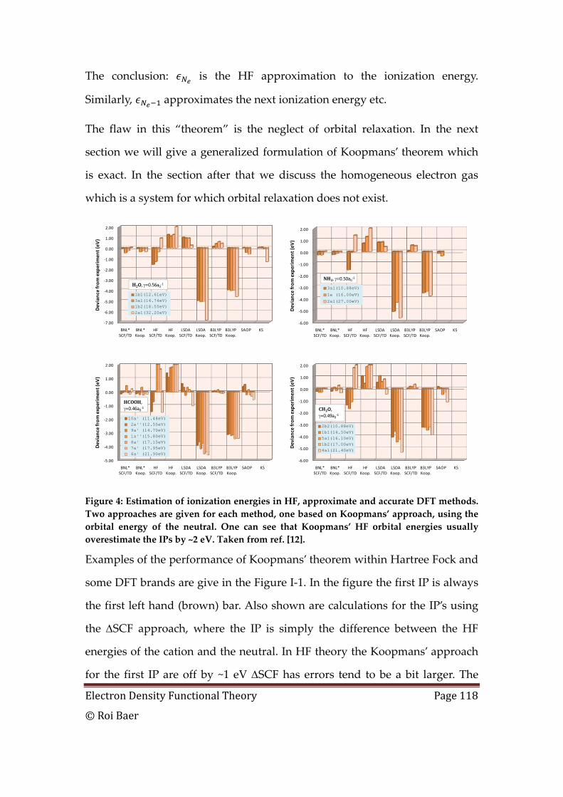
Electron Density Functional Theory Page 118
© Roi Baer
The conclusion: is the HF approximation to the ionization energy.
Similarly, approximates the next ionization energy etc.
The flaw in this “theorem” is the neglect of orbital relaxation. In the next
section we will give a generalized formulation of Koopmans’ theorem which
is exact. In the section after that we discuss the homogeneous electron gas
which is a system for which orbital relaxation does not exist.
Figure 4: Estimation of ionization energies in HF, approximate and accurate DFT methods. Two approaches are given for each method, one based on Koopmans’ approach, using the orbital energy of the neutral. One can see that Koopmans’ HF orbital energies usually overestimate the IPs by ~2 eV. Taken from ref. [12].
Examples of the performance of Koopmans’ theorem within Hartree Fock and
some DFT brands are give in the Figure I‐1. In the figure the first IP is always
the first left hand (brown) bar. Also shown are calculations for the IP’s using
the ΔSCF approach, where the IP is simply the difference between the HF
energies of the cation and the neutral. In HF theory the Koopmans’ approach
for the first IP are off by ~1 eV ΔSCF has errors tend to be a bit larger. The
‐7.00
‐6.00
‐5.00
‐4.00
‐3.00
‐2.00
‐1.00
0.00
1.00
2.00
BNL* SCF/TD
BNL* Koop.
HF SCF/TD
HF Koop.
LSDA SCF/TD
LSDA Koop.
B3LYP SCF/TD
B3LYP Koop.
SAOP KS
Deviance from
experim
ent (eV
)
1b1(12.61eV)3a1(14.74eV)1b2(18.55eV)2a1(32.20eV)
H2O, γ=0.56a0‐1
‐6.00
‐5.00
‐4.00
‐3.00
‐2.00
‐1.00
0.00
1.00
2.00
BNL* SCF/TD
BNL* Koop.
HF SCF/TD
HF Koop.
LSDA SCF/TD
LSDA Koop.
B3LYP SCF/TD
B3LYP Koop.
SAOP KS
Deviance from
experim
ent (eV
)3a1(10.88eV)
1e (16.00eV)
2a1(27.00eV)
NH3, γ=0.50a0‐1
‐5.00
‐4.00
‐3.00
‐2.00
‐1.00
0.00
1.00
2.00
BNL* SCF/TD
BNL* Koop.
HF SCF/TD
HF Koop.
LSDA SCF/TD
LSDA Koop.
B3LYP SCF/TD
B3LYP Koop.
SAOP KS
Deviance from
experim
ent (eV
)
10a' (11.48eV)2a''(12.55eV)9a' (14.70eV)1a''(15.80eV)8a' (17.15eV)7a' (17.95eV)6a' (21.90eV)
HCOOH, γ=0.46a0‐1
‐6.00
‐5.00
‐4.00
‐3.00
‐2.00
‐1.00
0.00
1.00
2.00
BNL* SCF/TD
BNL* Koop.
HF SCF/TD
HF Koop.
LSDA SCF/TD
LSDA Koop.
B3LYP SCF/TD
B3LYP Koop.
SAOP KS
Deviance from
experim
ent (eV
)
2b2(10.88eV)1b1(14.50eV)5a1(16.10eV)1b2(17.00eV)4a1(21.40eV)
CH2O, γ=0.49a0‐1

Electron Density Functional Theory Page 119
© Roi Baer
usual brands of DFT, such as LSDA, B3LYP have large Koopmans’ errors but
small ΔSCF errors. The brand called BNL has small errors in both respects.
C. Fractional occupation numbers, the HF orbital functional and the generalized Koopmans’
theorem
We now make a fundamental generalization of the Hartree‐Fock energy.
Instead of viewing it as an expectation value of a determinantal wave
function, we view it as a new fundamental concept: an orbital functional. We
take Eq. (4.1.9) and write it as a functional of “all” orbitals and occupation
numbers:
, , … ; , , …12 | |
(5.2.4)
Here the functional depends on an (in principle) infinite set of orthonormal
orbitals and their corresponding occupation numbers. Since electrons are
fermions each occupation number is limited to the unit interval, i.e. 0 1
(since you cannot have negative occupation and you cannot have more than 1
electron in a given orbital because of the Pauli principle). Let us minimize this
functional for electrons. What we mean by this is that we minimize this
energy with respect to the orbitals and the occupation numbers
under the constraints that the orbitals are orthonormal and the occupation
numbers are non‐negative, not greater than 1 and that they sum up to . Thus
the Lagrangian for this constraint minimization is
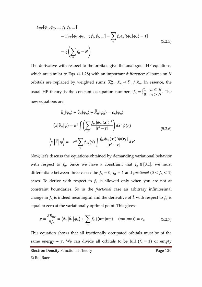
Electron Density Functional Theory Page 120
© Roi Baer
, , … ; , , …
, , … ; , , … | 1
(5.2.5)
The derivative with respect to the orbitals give the analogous HF equations,
which are similar to Eqs. (4.1.28) with an important difference: all sums on
orbitals are replaced by weighted sums: ∑ ∑ . In essence, the
usual HF theory is the constant occupation numbers 1 0 . The
new equations are:
| | | |
| || |
| |
(5.2.6)
Now, let’s discuss the equations obtained by demanding variational behavior
with respect to . Since we have a constraint that 0,1 , we must
differentiate between three cases: the 0, 1 and fractional (0 1)
cases. To derive with respect to is allowed only when you are not at
constraint boundaries. So in the fractional case an arbitrary infinitesimal
change in is indeed meaningful and the derivative of with respect to is
equal to zero at the variationally optimal point. This gives:
| | (5.2.7)
This equation shows that all fractionally occupated orbitals must be of the
same energy – . We can divide all orbitals to be full ( 1 or empty

Electron Density Functional Theory Page 121
© Roi Baer
( 0 and partially occupied but these latter orbitals all have the same
orbital energy. We have seen that for the Hartree‐Fock solution to be stable,
only the lowest orbitals can be occupied. Thus the picture that emerges is:
there are fully occupied orbitals. Then there can be several degenerate
orbitals with fractional occupation that adds up to (assuming is integer).
The rest of the orbitals are unoccied..
Eq. (5.2.7) is now an exact formulation of Koopmans’ theorem. Suppose we
have a system with slightly less than an integer number of electrons:
where is a small fraction. Then:
(5.2.8)
Where is the energy of the highest (can be partially) occupied orbital
for the ‐eletrons system. Thus we see that if we “slightly” ionize the system
Koopmans’ theorem holds exactly (in a sense, the change is so small that there
will be no orbital relxation). Of course, in real molecules there is no such
thing as a fractional electron. But still, in terms of the orbital HF theory there is.
This new concept of an orbital functional has allowed us to consider an exact
and generalized version of Koopmans’ theorem. We will see in later chapters
that orbital functionals play an important role in advanced approaches to
DFT.
D. Hartree-Fock for the homogeneous electron gas
i. Hartree-Fock orbitals and orbital energies of HEG
Let us now apply the Hartree‐Fock theory to an important system which is a
model for the valence electrons of a simple metal such as sodium. This is once
again the homogeneous electron, gas of electrons in a cubic box of volume
under periodic boundary conditions. Note that we are imposing on our
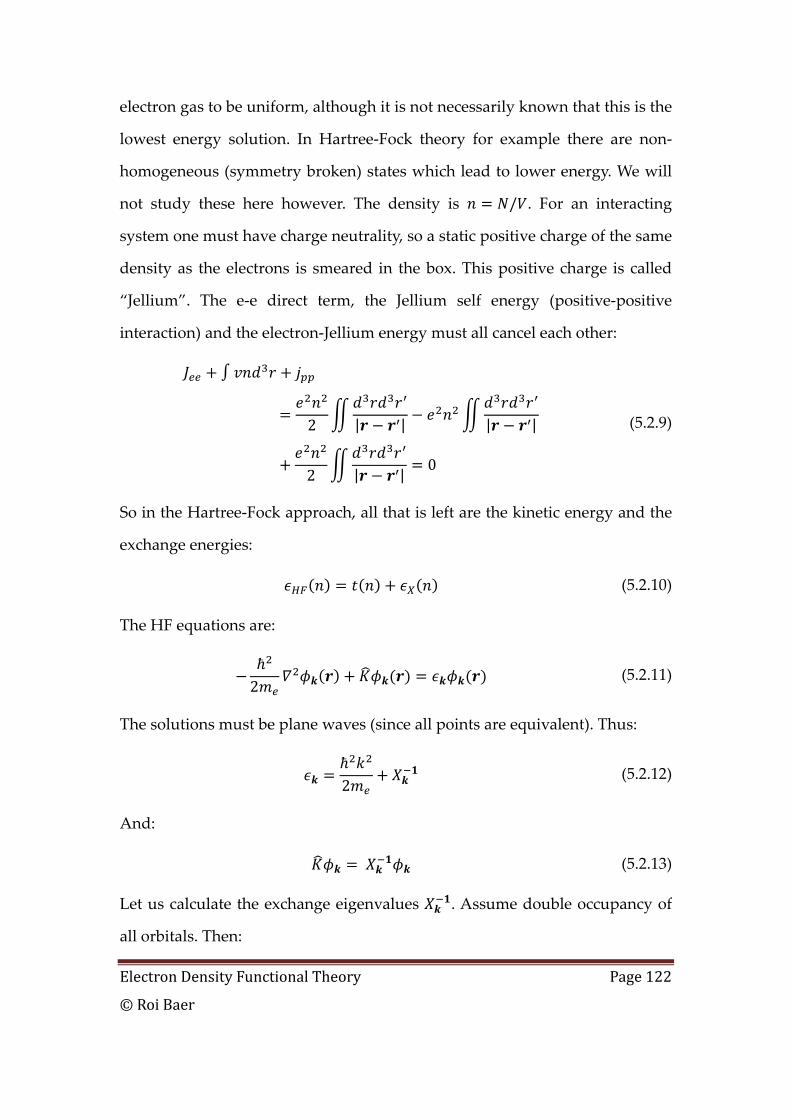
Electron Density Functional Theory Page 122
© Roi Baer
electron gas to be uniform, although it is not necessarily known that this is the
lowest energy solution. In Hartree‐Fock theory for example there are non‐
homogeneous (symmetry broken) states which lead to lower energy. We will
not study these here however. The density is / . For an interacting
system one must have charge neutrality, so a static positive charge of the same
density as the electrons is smeared in the box. This positive charge is called
“Jellium”. The e‐e direct term, the Jellium self energy (positive‐positive
interaction) and the electron‐Jellium energy must all cancel each other:
2 | | | |
2 | | 0
(5.2.9)
So in the Hartree‐Fock approach, all that is left are the kinetic energy and the
exchange energies:
(5.2.10)
The HF equations are:
2 (5.2.11)
The solutions must be plane waves (since all points are equivalent). Thus:
2 (5.2.12)
And:
(5.2.13)
Let us calculate the exchange eigenvalues . Assume double occupancy of
all orbitals. Then:
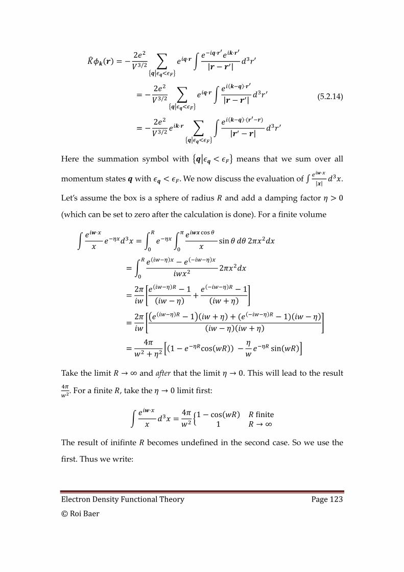
Electron Density Functional Theory Page 123
© Roi Baer
2/ | |
2/ | |
2/
| |
(5.2.14)
Here the summation symbol with means that we sum over all
momentum states with . We now discuss the evaluation of
| | .
Let’s assume the box is a sphere of radius and add a damping factor 0
(which can be set to zero after the calculation is done). For a finite volume
sin 2
2
2 1 1
2 1 1
41 cos sin
Take the limit ∞ and after that the limit 0. This will lead to the result
. For a finite , take the 0 limit first:
4 1 cos finite1 ∞
The result of inifinte becomes undefined in the second case. So we use the
first. Thus we write:
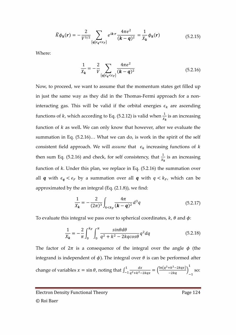
Electron Density Functional Theory Page 124
© Roi Baer
2/
4 1 (5.2.15)
Where:
1 2 4 (5.2.16)
Now, to proceed, we want to assume that the momentum states get filled up
in just the same way as they did in the Thomas‐Fermi approach for a non‐
interacting gas. This will be valid if the orbital energies are ascending
functions of , which according to Eq. (5.2.12) is valid when is an increasing
function of as well. We can only know that however, after we evaluate the
summation in Eq. (5.2.16)… What we can do, is work in the spirit of the self
consistent field approach. We will assume that increasing functions of
then sum Eq. (5.2.16) and check, for self consistency, that is an increasing
function of . Under this plan, we replace in Eq. (5.2.16) the summation over
all with by a summation over all with , which can be
approximated by the an integral (Eq. (2.1.8)), we find:
1 22
4 (5.2.17)
To evaluate this integral we pass over to spherical coordinates, , and :
1 22 (5.2.18)
The factor of 2 is a consequence of the integral over the angle (the
integrand is independent of . The integral over is can be performed after
change of variables sin , noting that so:
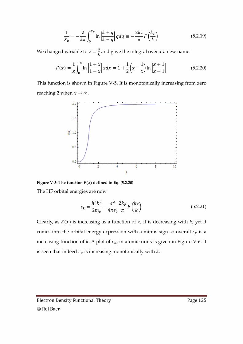
Electron Density Functional Theory Page 125
© Roi Baer
1 2ln
2 (5.2.19)
We changed variable to and gave the integral over a new name:
1ln
11 1
12
1ln
11
(5.2.20)
This function is shown in Figure V‐5. It is monotonically increasing from zero
reaching 2 when ∞.
Figure V‐5: The function defined in Eq. (5.2.20)
The HF orbital energies are now
2 42
(5.2.21)
Clearly, as is increasing as a function of , it is decreasing with , yet it
comes into the orbital energy expression with a minus sign so overall is a
increasing function of . A plot of , in atomic units is given in Figure V‐6. It
is seen that indeed is increasing monotonically with .

Electron Density Functional Theory Page 126
© Roi Baer
Figure V‐6: The Hartree‐Fock orbital energies for various values of (all in atomic units). For any given the function is increasing with .
Exercise: Determine the Hartree‐Fock density matrix of the HEG.
We have shown that the Hartree‐Fock orbitals are plane waves with wave
vectors less than . Thus:
,1
(5.2.22)
Denoting we find that depends only on and so:
212
22 2
22
4sin
12
8sin cos
sin cos
(5.2.23)
Since 3 we find:
3sin cos
(5.2.24)
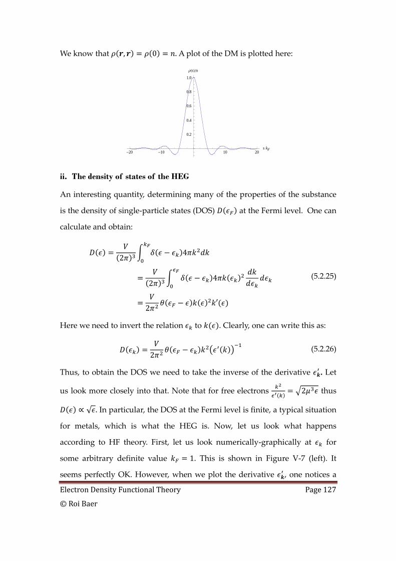
Electron Density Functional Theory Page 127
© Roi Baer
We know that , 0 . A plot of the DM is plotted here:
ii. The density of states of the HEG
An interesting quantity, determining many of the properties of the substance
is the density of single‐particle states (DOS) at the Fermi level. One can
calculate and obtain:
2 4
2 4
2
(5.2.25)
Here we need to invert the relation to . Clearly, one can write this as:
2 (5.2.26)
Thus, to obtain the DOS we need to take the inverse of the derivative . Let
us look more closely into that. Note that for free electrons 2 thus
√ . In particular, the DOS at the Fermi level is finite, a typical situation
for metals, which is what the HEG is. Now, let us look what happens
according to HF theory. First, let us look numerically‐graphically at for
some arbitrary definite value 1. This is shown in Figure V‐7 (left). It
seems perfectly OK. However, when we plot the derivative , one notices a
-20 -10 10 20s kF
0.2
0.4
0.6
0.8
1.0
rHsLên
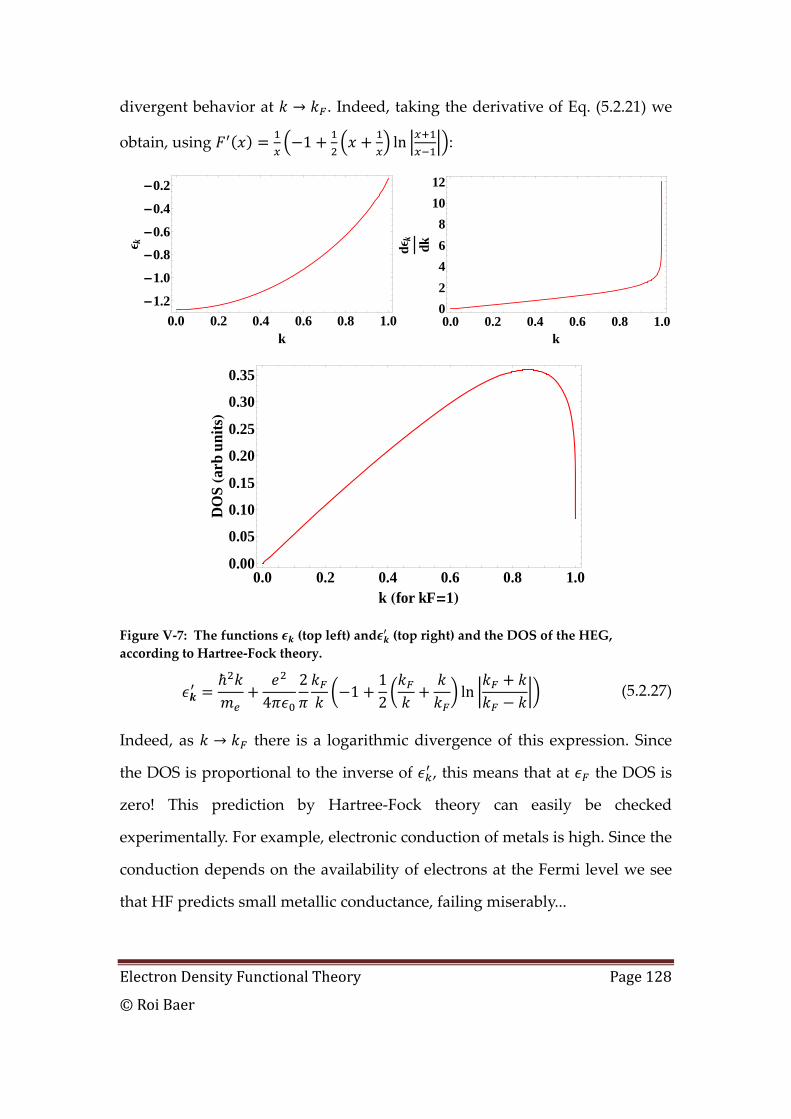
Electron Density Functional Theory Page 128
© Roi Baer
divergent behavior at . Indeed, taking the derivative of Eq. (5.2.21) we
obtain, using 1 ln :
Figure V‐7: The functions (top left) and (top right) and the DOS of the HEG, according to Hartree‐Fock theory.
42
112 ln (5.2.27)
Indeed, as there is a logarithmic divergence of this expression. Since
the DOS is proportional to the inverse of , this means that at the DOS is
zero! This prediction by Hartree‐Fock theory can easily be checked
experimentally. For example, electronic conduction of metals is high. Since the
conduction depends on the availability of electrons at the Fermi level we see
that HF predicts small metallic conductance, failing miserably...
0.0 0.2 0.4 0.6 0.8 1.0-1.2
-1.0
-0.8
-0.6
-0.4
-0.2
k
e k
0.0 0.2 0.4 0.6 0.8 1.002468
1012
k
dek
dk
0.0 0.2 0.4 0.6 0.8 1.00.00
0.05
0.10
0.15
0.20
0.25
0.30
0.35
k Hfor kF=1L
DO
SHa
rbun
itsL
Electron Density Functional Theory Page 129
© Roi Baer
iii. Stability of the HEG in Hartree-Fock theory
The density matrix assuming unpolarized gas (all electrons are spin‐paired) is
given by Eq. (5.2.24). Now, we can calculate the total exchange energy. From
Eq. (4.1.17):
14
,| |
4sin cos
4/
sin cos/
(5.2.28)
Notice that . Thus for
∞ which is the limit of large volume, we have:
sin cos 14
(5.2.29)
Thus for large volume:
4 (5.2.30)
From (2.1.15) so:
34 (5.2.31)
The exchange energy per particle is:
34
/ (5.2.32)
With /
0.73856. Let us recall the kinetic energy per particle for
the HEG (Eq. (2.1.18)):
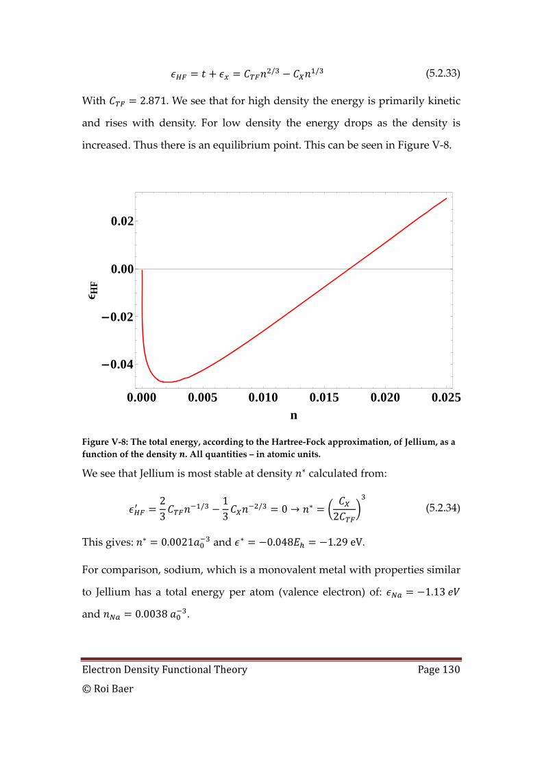
Electron Density Functional Theory Page 130
© Roi Baer
/ / (5.2.33)
With 2.871. We see that for high density the energy is primarily kinetic
and rises with density. For low density the energy drops as the density is
increased. Thus there is an equilibrium point. This can be seen in Figure V‐8.
Figure V‐8: The total energy, according to the Hartree‐Fock approximation, of Jellium, as a function of the density . All quantities – in atomic units.
We see that Jellium is most stable at density calculated from:
23
/ 13
/ 0 2 (5.2.34)
This gives: 0.0021 and 0.048 1.29 eV.
For comparison, sodium, which is a monovalent metal with properties similar
to Jellium has a total energy per atom (valence electron) of: 1.13
and 0.0038 .
0.000 0.005 0.010 0.015 0.020 0.025
-0.04
-0.02
0.00
0.02
n
e HF
Electron Density Functional Theory Page 131
© Roi Baer
VI. The Hohenberg-Kohn density theory
In view of the poor predictions of chemical bonds and molecular properties
afforded by HF approximation and the high numerical price of wave function
approaches, it is beneficial to seek out methods that circumvent the need to
represent the many‐body electronic wavefunction. We studied in detail two
theories. One was based on the density, but had no real rigorous basis. The
other was a method that assumed the electronic wave function is of the form
applicable only for non‐interacting electrons. We now want to describe a
rigorous method that combines ideas of this type in a new way which is both
rigorous and leads to very accurate approximations.
A. The first HK theorem
In electronic structure theory the Hamiltonian is given as:
(6.1.1)
Where all symbols have been defined in XXX. The identity of the molecular
system is captured in the external potential . The other terms are
“universal” i.e. the same for all molecules. In DFT they have a special symbol:
. (6.1.2)
Different Hamiltonians differ only by their external potential‐density term:
(6.1.3)
This observation has a fundamental implication. Suppose we have two
electronic wave functions Ψ and Ψ of electrons which have the same
density, i.e. for all :
Ψ | |Ψ Ψ | |Ψ . (6.1.4)
Now, if
Electron Density Functional Theory Page 132
© Roi Baer
Ψ Ψ Ψ Ψ (6.1.5)
Then:
Ψ Ψ Ψ Ψ (6.1.6)
Thus the inequality is independent of the position of the nuclei: only the wave
functions affect it through the universal operator . The external potential
term drops out because both wave functions have the same density.
An interesting natural conclusions is that if Eq. (6.1.5) holds for one
Hamiltonian the it holds for all Hamiltonians::
Ψ Ψ Ψ Ψ (6.1.7)
This fact will now be used to prove the first theorem of DFT, due to
Hohenberg and Kohn:
Theorem (Hohenberg‐Kohn): When two Hamiltonians differing only by a
single particle potential term have non
degenerate ground states which integrate to the same density then these
Hamiltonians are identical up to a constant (i.e. ).
Proof of the HK theorem: Assume otherwise: Ψ is the GS of and Ψ that of
, both wave functions assumed real and have the same expectation values
for the density at all points in space. The variational principle for Ψ dictates
Ψ Ψ Ψ Ψ which, as discussed in Eq. (6.1.7) means that Ψ Ψ
Ψ Ψ holds as well. But this latter inequality contradicts the variational
principle for Ψ as the ground state of , unless it differs from by at most a
constant.♦
This theorem allows one to think of the potential as a functional dependent on
the density. Thus, in addition to the “usual”
(6.1.8)
Electron Density Functional Theory Page 133
© Roi Baer
We now have:
(6.1.9)
Thus ʺeverythingʺ about the molecule (all its properties) is in the above sense
a functional of the ground‐state density.
A generalization of the theorem, giving an inequality is:
Theorem: If is the density of the non‐degenerate N‐particle groundstate
of , where 1,2. Then, denoting Δ , we
have:
Δ 0 Δ Δ 0 (6.1.10)
Proof: Suppose Δ 0. Then Ψ Ψ and because of non‐degeneracy the
following inequality is strict:
Ψ Ψ Ψ Ψ Ψ Ψ (6.1.11)
Denoting Ψ Ψ , we find:
Δ (6.1.12)
And exchanging the indices 1 2:
Δ (6.1.13)
Adding the two inequalities and cleaning up gives Eq. (6.1.10), QED♦
B. The HK functional
Since ʺeverythingʺ is a functional of the density, we can assert that the
ground‐state kinetic energy is a functional of the density and so is the
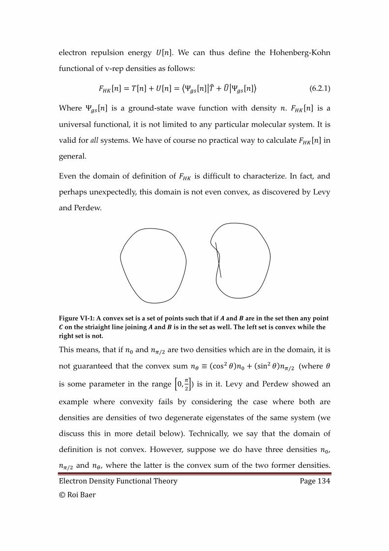
Electron Density Functional Theory Page 134
© Roi Baer
electron repulsion energy . We can thus define the Hohenberg‐Kohn
functional of v‐rep densities as follows:
Ψ Ψ (6.2.1)
Where Ψ is a ground‐state wave function with density . is a
universal functional, it is not limited to any particular molecular system. It is
valid for all systems. We have of course no practical way to calculate in
general.
Even the domain of definition of is difficult to characterize. In fact, and
perhaps unexpectedly, this domain is not even convex, as discovered by Levy
and Perdew.
Figure VI‐1: A convex set is a set of points such that if and are in the set then any point on the striaight line joining and is in the set as well. The left set is convex while the right set is not.
This means, that if and / are two densities which are in the domain, it is
not guaranteed that the convex sum cos sin / (where
is some parameter in the range 0, ) is in it. Levy and Perdew showed an
example where convexity fails by considering the case where both are
densities are densities of two degenerate eigenstates of the same system (we
discuss this in more detail below). Technically, we say that the domain of
definition is not convex. However, suppose we do have three densities ,
/ and , where the latter is the convex sum of the two former densities.
Electron Density Functional Theory Page 135
© Roi Baer
Suppose further that all three belong to the domain of definition of . Then
cos sin / , i.e. is a convex functional
of the density (we discussed this concept in Chapter XXX). This is seen as a
result of the variational theorem. Suppose Ψ is the ground‐state wave
function, the potential and the Hamiltonian
corresponding to then:
Ψ Ψ Ψ Ψ
Ψ Ψ Ψ / Ψ / (6.2.2)
From this we have:
Ψ Ψ
cos Ψ Ψ
sin Ψ / Ψ / /
cos sin /
(6.2.3)
We will see that the convextity property of has an important
implication for the variational property of density functional theory, that we
discuss in the next section.
C. Minimum principle for density functional theory
The second HK theorem establishes a minimum principle involving the
density, and it can be used to ʺfindʺ the density without direct reference to the
concept of a “wave function”.
Given a potential , consider the following functional for electrons:
(6.3.1)

Electron Density Functional Theory Page 136
© Roi Baer
The HK theorem II states that the density which is the ground‐state of
minimizes this functional. For we know of course that:
Ψ Ψ (6.3.2)
Where . HK theorem II states that for any other v‐rep density
of electrons:
(6.3.3)
The proof is an immediate consequence of tha quantum mechanical
variational principle:
Ψ Ψ Ψ Ψ (6.3.4)
This theorem allows one to speak of a ʺminimum‐principleʺ concerning the
density. If we have an approximate we can find an approximation to the
ground‐state density , simply by finding the minimum.
The fact that is convex (in the limited sense, since there is still the issue
of domain of definition discussed below), as proved in the previous section,
implies that is convex as well, since by adding a linear term to a
function one cannot change its convex/non‐convex character. The convexity is
desirable since it assures that the minimum is not only global, but that there
are no local minima as well, since a convex function (and functional) have no
truly local minima. There is still the problem of the convexity of the domain and
this spoils this useful conclusion. Below we show how to construct a
functional with a convex domain. But then, we lose the convex property of the
functional.
We now derive the basic equation of DFT (ignoring for the time being the
problem of convexity of the domain). We need to minimize under the
constraint that . Thus we need to minimize the Lagrangian:
Electron Density Functional Theory Page 137
© Roi Baer
, (6.3.5)
Where the value of is varied until the constraint is respected. The final
minimizing density obeys:
0 , (6.3.6)
This is the basic equation of DFT. It has no direct mention of the wave‐
function. Once we find an approximation for we can get an
approximation for from this equation.
The two theorems of HK put some rigor into the Thomas‐Fermi
approximation. In this KH theory is an approximation to and the
TF equations are an application of (6.3.5). Still, we know that TF theory is very
poor for chemistry. This means that despite the added rigor, the TF
approximation is too cumbersome for quantum chemistry.
D. An interesting observation on the variational principle of non-interacting electrons
Consider a system of non‐interacting particles in a potential . Usually
we may assume that the ground state of this system is a Slater wave function
Φ det … . The variational theorem states that their ground state
energy is given by minimizing:
| 1 (6.4.1)
Where , are Lagrange multipliers imposing the unit norm of
each orbital. Minimizing leads to the equations:
(6.4.2)
Electron Density Functional Theory Page 138
© Roi Baer
After solving for the lowest energy eigenstates the energy is ∑ ,
the kinetic energy is ∑ the density is
∑ | | .
Now consider a different problem. Suppose the density is given and one is
required to find the system with this density that has the minimum kinetic
energy . This leads to the Lagrangian:
| |
| 1
(6.4.3)
Now are Lagrange multipliers and must be searched for in order that the
constraint ∑ | | be fulfilled. After minimizing we obtain the
equations:
(6.4.4)
This equation rises from the attempt to compute and is the same as Eq.
(6.4.2) which rose as when was given and was calculated. This shows
that minimizing the kinetic energy under a given density invokes “the
same”equations as minimizing the energy when the potential is given. This
fact will be used in the Kohn‐Sham method.
E. The set of V-representabile densities
i. V-rep densities correspond to ground states wave function of some
potential well
The HK theorem shows that the ground state density of a system uniquely
determines the one body potential. This is a uniqueness statement: there is at
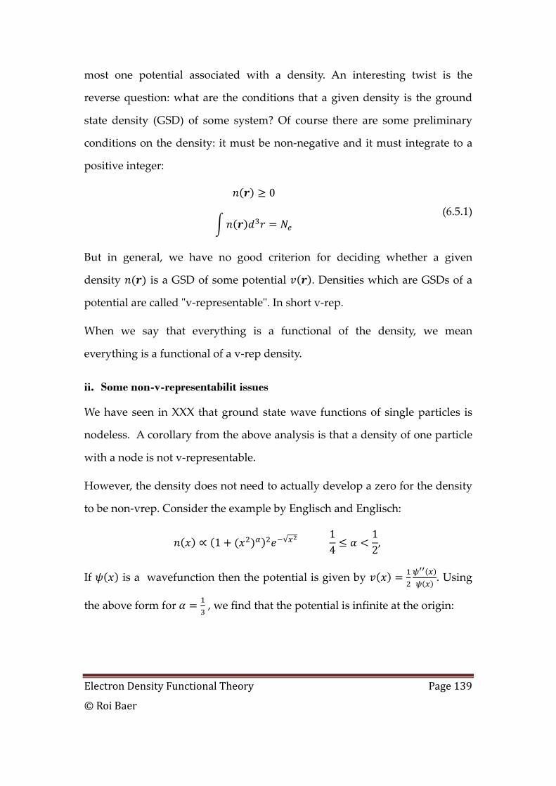
Electron Density Functional Theory Page 139
© Roi Baer
most one potential associated with a density. An interesting twist is the
reverse question: what are the conditions that a given density is the ground
state density (GSD) of some system? Of course there are some preliminary
conditions on the density: it must be non‐negative and it must integrate to a
positive integer:
0
(6.5.1)
But in general, we have no good criterion for deciding whether a given
density is a GSD of some potential . Densities which are GSDs of a
potential are called ʺv‐representableʺ. In short v‐rep.
When we say that everything is a functional of the density, we mean
everything is a functional of a v‐rep density.
ii. Some non-v-representabilit issues
We have seen in XXX that ground state wave functions of single particles is
nodeless. A corollary from the above analysis is that a density of one particle
with a node is not v‐representable.
However, the density does not need to actually develop a zero for the density
to be non‐vrep. Consider the example by Englisch and Englisch:
1 √ 14
12,
If is a wavefunction then the potential is given by . Using
the above form for , we find that the potential is infinite at the origin:
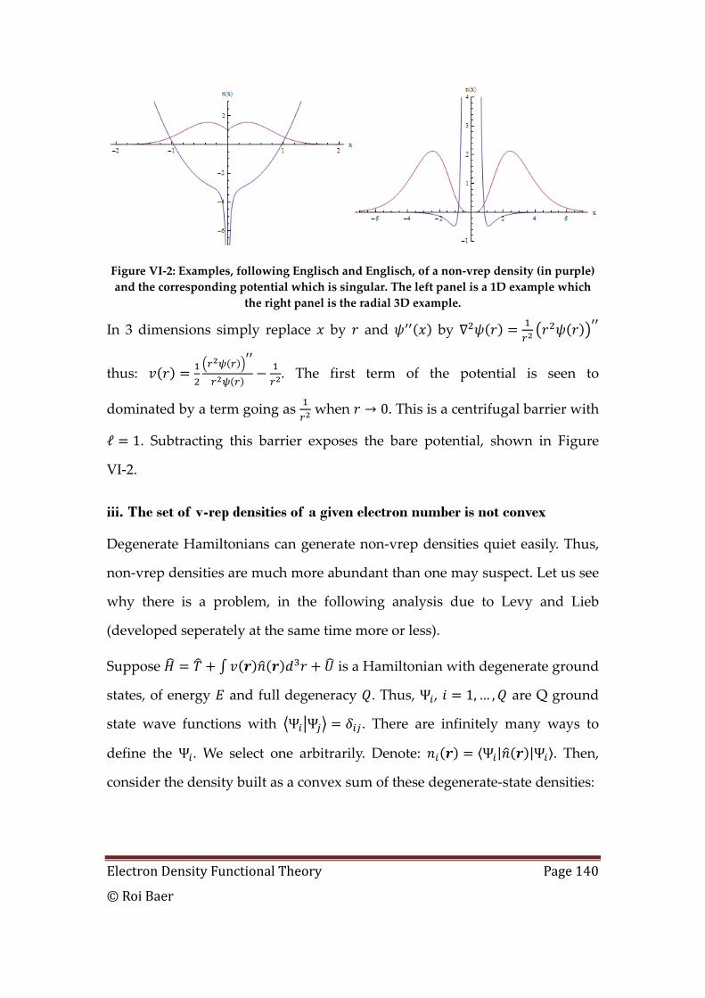
Electron Density Functional Theory Page 140
© Roi Baer
Figure VI‐2: Examples, following Englisch and Englisch, of a non‐vrep density (in purple) and the corresponding potential which is singular. The left panel is a 1D example which
the right panel is the radial 3D example.
In 3 dimensions simply replace by and by
thus: . The first term of the potential is seen to
dominated by a term going as when 0. This is a centrifugal barrier with
ℓ 1. Subtracting this barrier exposes the bare potential, shown in Figure
VI‐2.
iii. The set of v-rep densities of a given electron number is not convex
Degenerate Hamiltonians can generate non‐vrep densities quiet easily. Thus,
non‐vrep densities are much more abundant than one may suspect. Let us see
why there is a problem, in the following analysis due to Levy and Lieb
(developed seperately at the same time more or less).
Suppose is a Hamiltonian with degenerate ground
states, of energy and full degeneracy . Thus, Ψ , 1,… , are Q ground
state wave functions with Ψ Ψ . There are infinitely many ways to
define the Ψ . We select one arbitrarily. Denote: Ψ | |Ψ . Then,
consider the density built as a convex sum of these degenerate‐state densities:

Electron Density Functional Theory Page 141
© Roi Baer
0 1 (6.5.2)
We now show that this density it is usually non‐v‐representable. Of course, it
may happen (in rare cases) that a linear combination of the degenerate wave
functions Ψ ∑ Ψ yields Ψ| |Ψ . This case however is not
ordinary and we consider the cases where this does not happen. We thus
proceed to show that cannot be the groundstate density of any other
Hamiltonian as well. We do this by contradiction and assume existence of a
wavefunction Ψ which is the GS of some and such that Ψ | |Ψ
. The variational principle states Ψ Ψ Ψ Ψ for each .
Multiply by the positive (so the inequality is not spoiled) and sum over ,
using ∑ 1, and obtain ∑ Ψ Ψ Ψ Ψ . Now use the same
reasoning that led to Eq. (6.1.7) and replace by , obtaining:
∑ Ψ Ψ Ψ Ψ . However, Ψ Ψ and so this leads to
Ψ Ψ which condtradicts of the variational principle for Ψ . Hence,
Ψ cannot be the ground‐state of any Hamiltoian.
Example: The above theorem is general and holds for any system of particles. We consider non‐interacting electrons. Consider the density of non‐interacting electrons in the potential well created by a a Lithium nucleus. The ground state is 4‐fold degenerate Ψ |1 1 2 |, Ψ |1 1 2 |, Ψ 1 1 2 , Ψ |1 1 2 |
with √
, √
, √
, √
,
√. The 4 densities are: 2 , 2 , 2 , 2 . The average is given by:
14 2 128 2
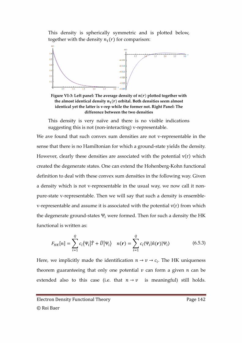
Electron Density Functional Theory Page 142
© Roi Baer
This density is spherically symmetric and is plotted below, together with the density for comparison:
Figure VI‐3: Left panel: The average density of plotted together with the almost identical density orbital. Both densities seem almost identical yet the latter is v‐rep while the former not. Right Panel: The
difference between the two densities
This density is very naïve and there is no visible indications suggesting this is not (non‐interacting) v‐representable.
We ave found that such convex sum densities are not v‐representable in the
sense that there is no Hamiltonian for which a ground‐state yields the density.
However, clearly these densities are associated with the potential v r which
created the degenerate states. One can extend the Hohenberg‐Kohn functional
definition to deal with these convex sum densities in the following way. Given
a density which is not v‐representable in the usual way, we now call it non‐
pure‐state v‐representable. Then we will say that such a density is ensemble‐
v‐representable and assume it is associated with the potential v r from which
the degenerate ground‐states Ψ were formed. Then for such a density the HK
functional is written as:
Ψ Ψ Ψ | |Ψ (6.5.3)
Here, we implicitly made the identification . The HK uniqueness
theorem guaranteeing that only one potential can form a given can be
extended also to this case (i.e. that is meaningful) still holds.
Electron Density Functional Theory Page 143
© Roi Baer
Furthermore, the minimum principle, i.e. that with the more general
obtains its minimum at the density corresponding to remains true.
F. Levy-Lieb generalization of the HK functional
The minimum principle of HK is of crucial importance for density functional
theory. Yet, the basic equation (Eq. (6.3.6)) which is the basis for development
of DFT into a practical approach is somewhat problematic from the
mathematical point of view. In order to define the functional derivative, one
must ensure that there is an “open” neighborhood of the ground state density
for which can be defined for any density. As we saw, there is a
fundamental problem is that of v‐representability. The ensemble v‐
representability solved one kind of problems but it is not clear if there may be
additional classes of non‐v‐representability. It is not possible to assume that
any density that is positive and integrates to an integer is a density of a
ground state wave function of a Hamiltonian. Furthermore, we cannot even
assume that around a v‐representable density there is an “open
neighborhood” of v‐representabile densities.
In general one cannot waive the possibility that there may be densities which
are not the ground state densities of any system and still are arbitrarily close
to any of interest. In such a case the functional derivative of is
formally undefined.
A way around these problems, developed separately by Levy and by Lieb is
to formulate a functional defined for any density on the one hand and
equal to for v‐representable densities on the other which still allows
for the same type of minimum principle as does the HK functional. We first
Electron Density Functional Theory Page 144
© Roi Baer
note an important property of . We say that the wave function Ψ
realizes the density (and symbolize this as Ψ ) if:
Ψ| |Ψ Ψ (6.5.4)
We will now show that for any wavefunction Ψ which realizes
Ψ Ψ Ψ (6.5.5)
This is a direct result of the variational principle:
Ψ Ψ Ψ Ψ Ψ Ψ .
From this development we see also that the wave‐function which realizes this
minimum is the ground‐state wave function and is denoted Ψ . One has
therefore:
min Ψ Ψ (6.5.6)
Levy and Lieb decided to use this relation, valid only for v‐rep densities as the
definition of their functional, valid for any density:
min Ψ Ψ (6.5.7)
Exercise: Show that for any density there is at least one wave function which realizes it
Solution: For a one‐electron case this is trivial, since the density is non‐negative we can take the wave function as Ψ . For electrons, just “slice” to non‐overlapping parts each: positive, integrating to 1: (1) ∑ , 2 0, (3) where , and (4)
1. This can be done in countless ways (with a good sharp knife). Then the determinant Ψ … , is a wavefunction which creates .
Electron Density Functional Theory Page 145
© Roi Baer
The above exercise shows, that the definition in Eq. (6.5.7) makes sense for
practically all densities. One can now use instead of in Eq. (6.3.1)
and convert the Hohenberg‐Kohn minimum principle to a variational‐
minimum principle. The search for the constrained minimum can be done
using a Lagrange multiplier approach. We formulate the Lagrangian:
Ψ, , Ψ Ψ Ψ| |Ψ (6.5.8)
Given , one now find suitable Lagrange multipliers such that when
minimizing with respect to an antisymmetric wave function Ψ leads to the
constraint Ψ| |Ψ at any . The search for a minimizing wave
function will cease when the gradient is zero, so a necessary condition is:
Ψ Ψ, , | LL, 0 ΨLL
ΨLL (6.5.9)
Thus, when is given, the Lagrange multiplier function that
imposes the condition defines a Hamiltonian .
Note that is determined by the procedure up to a constant. If is v‐
rep then necessarily, by Kohn’s theorem, and Ψ is the
groundstate wave function. However, we are not in general assured that ΨLL
is always the ground state, since is not necessarily v‐rep. Indeed, from
(6.5.9), all we can say is that ΨLL must be some eigenstate of .
Once the minimum is attained, one can take the functional derivative of by
. As with any constrained minimization, when the derivative of the
optimized solution is taken with respect to the constraints, one obtains the
Lagrange multiplied (see (1.11.23)):
Electron Density Functional Theory Page 146
© Roi Baer
Ψ, , (6.5.10)
Now, once the constrained minimum has been found, one can plug into
the HK scheme and consider the Lagrangian corresponding to
:
(6.5.11)
If now one searches for the density that minimes this functional one
immediately obtains:
0 (6.5.12)
Showing that the minimum of is obtained when the density found
admits, as Lagrange multiplier , the same potential as was give to start
with , up to a constant.
Even with the LL functional one problem is still not solved: convexity. While
the domain of definition is now finally convex, the functional has lost
convexity. A counterexample for convexity can be given, using the degenerate
system used above to prove that the domain of definition of the HK functional
is non‐convex. Indeed, for that system, which had a potential and
degenerate eigensstates Ψ ( 1, … , ) all of energy :
Electron Density Functional Theory Page 147
© Roi Baer
c
Ψ T U V Ψ
(6.5.13)
Showing that for these densities the functional is concave (while for the case
where and ∑ are all v‐rep the functional is convex). Therefore overall
the functional is not convex.
Once again, it is possible to circumvent this problem by extending the
definition to ensemble densities.
Exercise: Discuss the Levy approach for a given density of a system of non‐interacting electrons.
In this case the Hamiltonian is i.e. a 1‐body Hamiltonian. Suppose , 1,2, … are the 1‐particle states which are eigenstates of :
2
(6.5.14)
Let us suppose orbital energy ordering, so that … If the density is “non‐interacting v‐rep” then it must be due to the Slater wave function of the lowest energy orbitals. In this case, the kinetic energy is given by:
(6.5.15)
And the functional derivative is:
Electron Density Functional Theory Page 148
© Roi Baer
(6.5.16)
If we are given a non‐interacting non‐v‐rep density then we might find not a ground state but an excited determinant, for example: . This leads to “holes” in the non‐interacting system.
G. The dilation inequality for the HK functional
We have already seen the the HF functional is convex. More exact properties
are desirable, so that when one derives approximations to this functional, they
can perhaps be forced to obey the known exact relations. One approach is to
use dilation considerations. This will lead to an interesting inequlaity.
We will use the following symbol convention:
Ψ , … , / Ψ , … ,
(6.6.1)
It is quite straightforward to show the following relations:
Exercise
Derive the following relation
Ψ | |Ψ Ψ| |Ψ
Ψ Ψ Ψ Ψ
Ψ Ψ Ψ Ψ
(6.6.2)
From the first relation in this equation, one can deduce that if Ψ (i.e. Ψ
is a many‐electron wave function exhibiting the spatial density ) then:
Ψ | |Ψ Ψ| |Ψ (6.6.3)
One can now also use this relation to get a dilation inequality. Indeed, since
Ψ realizes the density (see the first of Eqs. (6.6.2)) we have
Electron Density Functional Theory Page 149
© Roi Baer
Ψ Ψ Ψ Ψ Ψ Ψ , thus we
find:
(6.6.4)
VII. The Kohn-Sham method
Kohn and Sham noticed that the HK theory is valid for both interacting and
non‐interacting electrons. Now, they ask, what happens if for any system of
interacting electrons, with density there is a non‐interacting system of the
same density? It is clear that if such two systems exist they are unique. The
non‐interacting system has one advantage over the interacting system: we can
find its ground‐state rather easily, since the many‐body wavefunction is a
Slater wave function. So, the problem is: how to perform such a mapping.
A. Non-interacting electrons
If non‐interacting electrons are tractable, let then study their density
functionals. First, if we are given we assume it is non‐interacting v‐
representable. That is we assume there exists a potentials such that the
ground‐state of the resulting non‐interacting Hamiltonian admits
a ground‐state having as density. We can later use the Levy‐Lieb
approach to patch up the v‐representability requirement.
Let us denote the ground‐state wave function of non‐interacting electrons that
have the density by Φ . The Hohenberg‐Kohn functional for non‐
interacting electrons is reduced to just the kinetic energy, i.e. we define:
Φ Φ (7.1.1)
Electron Density Functional Theory Page 150
© Roi Baer
An interesting question is – can we devise a method to compute . For
most densities, the non‐interacting wave function is simply a Slater wave
function. The minimum principle for (derived from Eq. (6.5.5)) is:
Ψ Ψ Ψ (7.1.2)
One should not treat this equation lightly and realize its non‐trivial
consequences: that the ground‐state wave function of non‐interacting particles
associated with minimizes the kinetic energy! Let us see some
consequence this minimum principle.
Let Φ be the ground state wave function of the system of non interacting
electrons realizing the density . From the first equation in Eq. (6.6.2) one
sees that Φ realizes , thus one can plug it into the right hand side
of Eq. (7.1.2), with plugged into :
Φ Φ Φ Φ (7.1.3)
Since now the right hand side is an expression of a scaled wave‐function, one
can use Eq. (6.6.2) and obtain:
Φ Φ Φ Φ (7.1.4)
And so . But we can also use this equation to scale back to
by dilating by 1/ , since: /
. Then, the same rule applies and we
get: , and so . We obtained two contradicting
equations which can agree only if both are reduced to equality. Thus:
. (7.1.5)
This should be compared with the analogous result of Eq. (6.6.4) which is an
inequality. The dilation effects for non‐interacting electrons is obviously much
simpler. One important corollary of (7.1.5) is that the non‐interacting wave
Electron Density Functional Theory Page 151
© Roi Baer
functions scale with the density. This can be seen if one remembers that
Φ minimizes the kinetic energy. Therefore any function Φ for which
Φ Φ equals must be the ground state of the non‐interacting
system with density . We saw that Φ gives the correct kinetic energy of
for the system with density , , and therefore, necessarily:
Φ Φ . (7.1.6)
Exercise
1) We can define a functional called the Hartree energy, which is the
classical electrostatic energy associated with the charge distribution
:
| | (7.1.7)
Prove the following dilation relation:
(7.1.8)
2) Now define the exchange energy functional (see also Eq. (4.1.17) for a
definition based on the orbitals):
Φ Φ (7.1.9)
Use (7.1.6). Prove:
(7.1.10)
What is the relation between the potential for which is a non‐
interacting ground state density and , for which is a non‐
interacting ground state? We can use the basic DFTequation to answer this.
From the basic definition of functional derivation:
Electron Density Functional Theory Page 152
© Roi Baer
µ , lim (7.1.11)
The 3D delta‐function has the density dilation structure:
, so:
µ , lim (7.1.12)
Then using Eq.:
µ , lim
(7.1.13)
By dilating in the reverse direction we can easily see that:
µ
, (7.1.14)
We could have obtained this result directly from the Schrödinger equation.
Suppose Ψ is a many‐body eigenfunction of Hamiltonian ,
i.e Ψ Ψ. Define a scaled wavefunction:
Ψ ,… , Ψ ,… , (7.1.15)
Then clearly:
Ψ Ψ Ψ (7.1.16)
And so Ψ obeys the S. E. Ψ Ψ with energy and potential given by:
(7.1.17)
Electron Density Functional Theory Page 153
© Roi Baer
For a ground state of non‐interacting the first equation means that ,
is the one‐particle potential for the scaled determinant, and thus for
the scaled density (since the scaled determinant realizes the scaled density).
B. Orbitals for the non-interacting electrons
Consider the ground state wave function for the non‐interacting electrons
Φ . Suppose the non‐interacting electrons reside in the potential (the
subscript is in honor of Slater) then Φ Φ . In most
cases this wave function is a normalized Slater wave function. The only
exception might be the existence of a degeneracy and then there may be
several independent Slater wave functions and Φ is a linear combination.
However, one can always assume that he is looking for one of the
determinants and not for a linear combination (this means that one must be
careful not to impose possible symmetries of the Hamiltonian). Once one
does that, we can introduce orthormal spin‐orbitals 1… , from
which Φ is built. These orbitals are excited states of the potential well in
which the non‐interacting electrons reside. Thus the orbitals must each obey
the single‐electron Schrödinger equation:
2 (7.1.18)
The orbitals correspond to the lowest eigenvalues . The fact that Φ
realizes the density is expressed as :
(7.1.19)
The non‐interacting kinetic energy is then:
Electron Density Functional Theory Page 154
© Roi Baer
2 (7.1.20)
When one wants to find the functional derivative of with respect to
one can turn to basic equation, Eq. (6.3.6) which in case of non‐interacting
electrons becomes:
(7.1.21)
We will see that this equation is important for the method known as the
Kohn‐Sham method.
Note that the discussion of dilation in the previous subsection can be carried
on to the orbitals. The only additional information to convey is that the
orbitals scale as the density and each of the orbital energies scale as the total
energy:
, (7.1.22)
C. The correlation energy functional: definition
and some formal properties
The ground state energy of the an system of electrons in density can be
written in terms of the non‐interacting (Slater wave function) wave function
Φ :
Φ Φ (7.2.1)
This equation is actually a definition of a new density functional, the
correlation energy functional . If we suppose for the time being that
is known, this expression can be used to define a working procedure
for DFT known as the Kohn‐Sham method. From our studies of the Hartree‐

Electron Density Functional Theory Page 155
© Roi Baer
Fock theory, we know that the expectation value of within a determinant
can be written as:
Φ Φ (7.2.2)
Where is the Hartree energy:
2 | | (7.2.3)
And is given in terms of the orbitals from which Φ is composed (Eq.
(4.1.17)):
2| , || | (7.2.4)
Based on this, we rewrite as:
Ψ Ψ Φ Φ (7.2.5)
This allows us to write Eq. (7.2.5) compactly as:
(7.2.6)
Clearly we have also the equivalent equation:
(7.2.7)
Physical intuition concerning molecules and solids tells us that is a
small quantity when compared to or . Thus, it is reasonable to look
for approximations to this quantity. Approximation to the correlation energy
functional is the most important issue in DFT. It is an open question, still
being worked upon.
We shall deal with approximations later. Meanwhile, let us ask what can be
safely said about the correlation functional. We prove here several important

Electron Density Functional Theory Page 156
© Roi Baer
inequalities. First, consider the difference , the correlation
kinetic energy.
Exercise
Show is a positive quantity. This is actually intuitively clear: the
interacting electrons must have much more complicated ʺpathsʺ in the
interacting case because they want to avoid ʺbumping intoʺ other electrons.
Anything with more swirls must have higher kinetic energy.
Solution
Using the variational theorem:
Φ Φ Ψ Ψ
(7.2.8)
Where Ψ is the interacting ground‐state wave function determined by .
Comparing the two sides we have:
(7.2.9)
Next, we can show that the exchange correlation energy is always negative.
This comes about from our experience with expectation values of
determinants:
Φ Φ (7.2.10)
Using Eq. (7.2.6) we find:
0 (7.2.11)
Furthermore is negative as can be seen from the fact that is negative and is positive:
0 (7.2.12)
An additional property is the dilating relations. We have proved that and , . Thus:
Electron Density Functional Theory Page 157
© Roi Baer
(7.2.13)
One way to proceed is to substitute with . The other is to substitute with . We obtain from each possibility:
1
1 (7.2.14)
And, since is always positive and negative, we find that:
1
1 (7.2.15)
Obviously, the second relation is contained in the first (since 0) and so only the first relation is important; it can be used to derive complementary inequalities. Indeed, applying them for we find:
/ 1 (7.2.16)
This holds for any , so we stick in (7.2.16) instead of and using the fact that
/ to obtain:
1 (7.2.17)
D. The Kohn Sham equations
i. The Kohn-Sham equation from a system of non-interacting problem
Let us now turn to the issue of determining , required for the mapping
between the interacting non‐interacting systems. Let us start form the basic
equation Eq. (6.3.6) which becomes, using Eq. (7.2.6):
(7.3.1)
Where:
(7.3.2)
Electron Density Functional Theory Page 158
© Roi Baer
is the Hartree‐Exchange potential. Notice that:
| | (7.3.3)
and:
(7.3.4)
Thus, from Eq. (7.1.21) and Eq. (7.3.1) (up to a constant):
(7.3.5)
This equation gives us the potential of the non‐interacting system. Thus, we
have made a definite connection between the interacting and non‐interacting
systems.
Now, an important observation allows us to set up a simple method for
obtaining the ground‐state of an interacting system of electrons. We need to
find a density that obeys two conditions:
a) It is the density of the non‐interacting electrons so it is the sum of square
orbitals (Eq. (7.1.19)) that obey the Schrödinger equations (7.1.18) with
potential .
b) The potential must be related to the interacting system by Eq. (7.3.5)
This leads to a simple SCF procedure, called ʺThe Kohn‐Sham methodʺ
reminiscent of the Hartree‐Fock algorithm:
1. Guess . 2. Build , from (Eq. (7.3.3) and (7.3.4)). 3. Obtain the orbitals from the lowest eigenvalues of Eq. (7.1.18). 4. Compute the density from Eq. (7.1.19) 5. Redo from step 2 using the new density until you converge – i.e. until
the density changes no more.
Electron Density Functional Theory Page 159
© Roi Baer
When the process convergence, we have the exact ground‐state density .
It can be used to compute the ground‐state energy by plugging it into the
energy functional of Eq. (6.3.1):
(7.3.6)
ii. Systems with partially occupied orbitals
Partially occupied orbitals arise in the realm of ensemble‐DFT, i.e. when the
density searched for is not “non‐interacting v‐representable”. We still assume
the density is a sum of orbital densities as follows:
, (7.3.7)
but unlike Eq. (7.1.19) we do not impose exactly orbitals. The orbitals are
almost completely unconstrained, except for the Fermionic condition, that
their norm must be not be great than 1:
1, (7.3.8)
but the total number of electrons is still :
(7.3.9)
And the kinetic energy is written similarly to Eq. (7.1.20):
2 (7.3.10)
We generalized Eqs. (7.1.19) and (7.1.20) any number of orbitals leading to the
following orbital Lagrangian:
Electron Density Functional Theory Page 160
© Roi Baer
,
(7.3.11)
1,2, … and are Lagrange multipliers assuring orbital normality and
total number of particles. We minimize the Lagrangian with respect to the
orbitals and the occupation numbers (constraint to be non‐negative and
not greater than 1). The constraint minimum procedure thus requires that:
0 0 (7.3.12)
The first equation leads to the KS equations:
2 (7.3.13)
For convenience, we order the indexing so that the series of orbital energies is
ascending: The orbitals are now eigenfunctions of a Hermitian
Hamiltonian, and so we can assume they are orthogonal:
, (7.3.14)
We define as a short‐hand notation (see Eq.
(7.3.5)). By multiplying Eq. (7.3.13) by integrating on and summing on
q we find:
(7.3.15)
The second condition for minimum of holds only in cases that the
minimum is attained with non‐integer electron number, 1. The cases
Electron Density Functional Theory Page 161
© Roi Baer
1 or 0 are the boundary of the constraints and the derivative need
not be zero there. From this second part of the equation, we have:
, 0 1 (7.3.16)
This shows that all incompletely occupied orbitals have the same orbital
energy equal to the chemical potential , the Lagrange multiplier imposing
the number of particle constraint of the Hohenberg‐Kohn theory (Eq. (6.3.6)).
Typically, all orbitals with are fully occupied ( 1 and those with
are fully unoccupied ( 0 . The interacting electron energy is
obtained using Eqs. (7.3.6) and (7.3.15) as
– (7.3.17)
We should note that the development here assumed non‐interacting v‐
representability. In cases where this is not valid other occupation rules may
apply.
iii. Is the ground state wave function of non-interacting particles always a
Slater wave function
The standard KS approach to the non‐interacting kinetic energy is by defining
the functional as a minimum principle on the manifold of single
determinants:
min Φ Φ (7.3.18)
Setting up a Lagrangian and searching for the constrained minimum yields
occupied orbitals. If the density is not v‐representable one or more of the low
energy orbitals may have 0 occupation numbers.
Electron Density Functional Theory Page 162
© Roi Baer
Another way to define a non‐interacting kinetic energy functional is by an
extended minimum search over more general wave functions:
min Ψ Ψ (7.3.19)
Usually this search ends with Ψ being a single Slater wave function and for
these case and given are the same. Yet, this may not always be the case.
Let us assume that we are searching through all Ψ cos Φ sin Φ
where Φ or Φ are Slater wave functions. In general, the kinetic energy is
then:
min ΦA ΦA cos sin 2 ΦA ΦB
ΦB ΦB sin (7.3.20)
Now, if Φ and Φ differ by only one orbital (say for 1,… , 1 )
then Ψ is actually a Slater wave function: its orbitals are the 1 ’s and
then a new orbital cos sin is added. Next, if Φ and Φ
differ by two (or more) orbitals the cross term in (7.3.20) is zero and the
kinetic energy is simply the sum of orbitals kinetic energies with occupation
numbers given by cos and sin . The orbitals shared by the two
determinants will have unity occupation number (since cos sin 1)
while orbitals in the determinant but not in the B determinant will have
occupation number cos and those in the determinant but not in the A
determinant will have occupation number sin . The orbitals coming out
from the minimization will all solve a Schrödinger equation with the same
potential. The 4 odd orbitals (2 from each determinant) will all have the same
orbital energy equal to . When there are more than 2 Slater wavefunctions a
similar treatment will result and even more orbitals will be degenerate at the
Electron Density Functional Theory Page 163
© Roi Baer
chemical potential. Even if is v‐representable this type of wave function can
arise.
A third way to define the kinetic energy is as an ensemble average. Instead of
a wave function, one uses a mixed density matrix ∑ |Φ Φ |. The
constants are positive and sum to 1. The density is the convex sum
∑ of densities from each participating determinant. A similar
expression will arise for the kinetic energy. This approach is designed to solve
the problems of non‐interacting v‐representability emanating from convex
sums of degenerate wave functions (see section XXX).
iv. Janak’s Theorem
A very general theorem was noted by Janak [13], based on earlier work of
Slater and Wood[14] concerning the meaning of orbital energies. Let us return
to the functional of Eq. (7.3.11) and assume now that the occupation numbers
are given and they are all non‐negative and not larger than 1 and that they
sum up to the number of electrons. Thus, for a given set of occupation
numbers we can search for the orbitals that minimize the following
functional:
(7.3.21)
The equations that the orbitals must obey are still derived from Eq. (7.3.12)
leading to the same equations as in (7.3.13), the KS equation. Now, let us ask:
what happens to the energy when we change the occupation number of one
of the orbitals by an infinitesimal amount ? When we do this the “total
number of electrons” changes by this amount as well. This is not a physical
change (since electrons cannot change by non‐intereger amounts) but still
Electron Density Functional Theory Page 164
© Roi Baer
mathematically speaking the change can be studied. Since are the
constraints and the Lagrange multipliers in a minimization problem we can
use the general result of Eq. (1.11.23) that the rate at which the minimized
function changes when the constraints change is equal to the Lagrange
multiplier:
(7.3.22)
This relation, giving some meaning to the orbital energies is called Janak’s
theorem. This theorem is quite general but relies on some analytical
assumptions of the energy functional. For example, when the occupation
number is 1 the change can only be by a negative amount and when it is zero
– only positive. For approximate functionals, that are analytical with respect
to any and this relation holds. Such is the case for the often used
local, semilocal and even most hybrid functionals, including Hartree‐Fock
theorem.
In the conext of Hartree‐Fock theory this result is a restatement of Koopmans’
theorem, by which – is the unrelaxed ionization energy from orbital . The
orbital relaxation is a second order effect and thus negligible when occupation
numbers change infinitesimally.
E. “Virial Theorem” related identities in DFT
The following development is inspired by the virial theorem treatment. It
continues to consider dilation relations. Taking the derivative of with
respect to , we have 3 and since,
3 , we find
Electron Density Functional Theory Page 165
© Roi Baer
(7.4.1)
For a general density functional, , we have, using the chain rule for
derivatives, / and Eq. (7.4.1)then:
From which a completely general virial‐dilation relation holds for any
functional:
0 (7.4.2)
We will be especially interested in the case of 1. Thus the basic relation:
0 (7.4.3)
We further find that
(7.4.4)
Let us apply this for the Hartree energy. From Eq. (7.1.8) we find the following
relation, valid for any : 0, so:
0 (7.4.5)
A similar relation, namely 0 hold also for the exchange
energy (see Eq. (7.1.10)), and so:
3 0 (7.4.6)
Where / is the exchange potential.

Electron Density Functional Theory Page 166
© Roi Baer
Now, what about the correlation energy? Let us consider the KS DFT
functional:
(7.4.7)
Suppose is the density minimizing minimizer of and now plug into
the latter the scaled density. This will give a dependent energy:
(7.4.8)
And clearly, the minimum is at 1 so:
1 0 (7.4.9)
Now, let us evaluate using Eq. (7.1.5):
2 , (7.4.10)
and plug in 1. We obtain:
2 . (7.4.11)
or, using Eq. (7.4.3):
2 (7.4.12)
The second term in the parenthesis can be related to the interacting system.
Indeed we have, using Eqs. (6.6.2):
Ψ Ψ Ψ
Ψ Ψ (7.4.13)
Taking the derivative with respect to , remembering that Ψ 0 we
find, for 1:

Electron Density Functional Theory Page 167
© Roi Baer
0 2 Ψ Ψ (7.4.14)
(As a sidenote, you can see that substituting this relation in Eq. (7.4.1) gives
after trivial manipulation the virial theorem 2 Ψ Ψ
). Continuing the above development, using Eqs. (7.4.11) and
(7.4.14) we finally find:
| 2 , (7.4.15)
which can be written equivalently as:
| , (7.4.16)
or, using Eq. (7.4.3):
3 0. (7.4.17)
The Hartree and exchange energies give zero while the correlation energy
gives a negative quantity equal exactly to .
This result shows that the correlation energy functional and the correlation
potential are enough for determining the correlation kinetic energy (and from
it, by ) the kinetic energy itself.
This latter result is related to the virial theorem of Slater, which shows that
one can derive the kinetic energy of the electrons from the Born‐Oppneheimer
potential surface itself (Eq. (1.9.30)). Since DFT gives, in principle the Born‐
Oppenheimer potential surface, one can access the kinetic energy (and the
potential energy) from the DFT calculation.
Electron Density Functional Theory Page 168
© Roi Baer
F. Galilean invariance
A basic property of the electron‐electron interaction is that if the coordinates
of all electrons are shifted by a constant :
(7.5.1)
the e‐e interaction enegy does not change
12
1| |
12
1| | (7.5.2)
This property is shows that the e‐e interaction is translationally invariant. This
property is also called Galilean invariance. The same property holds when the
coordinates of each electron are rotated around some axis. This roatation can
be described by a 3×3 orthogonal matrix , where :
(7.5.3)
The lengths of vectors are preserved under a rotation:
| | | | (7.5.4)
Thus the e‐e interaction enegy does not change
12
1| |
12
1| |
12
1| |
12
1| |
(7.5.5)
Thus the e‐e energy is rotational invariant.
These relations indeed hold for the density functional since it is a
reflection of the e‐e functional. Indeed, define the shifted density:
(7.5.6)
Then:
Electron Density Functional Theory Page 169
© Roi Baer
12 | |
12 | |
(7.5.7)
We now make a variable replacement: and obtain:
12 | |
12 | |
(7.5.8)
This condition, that is called Galilean invariance. It is easy to
show that functional is also rotational invariant.
The exchange energy is also Galilean invariant, since the translation of the
density will cause a translation of the density matrix:
, , (7.5.9)
It is easy based on this to show that .
Finally, the same will hold for the kinetic energies , . All this shows
that we must demand this invariance of the correlation energy:
(7.5.10)
One consequence is the property of Galilean covariance of the potentials for
each of the above energy functionals. For example, for the correlation energy
we have the following result. Suppose we shift the density by a small
displacement:
Thus:
Electron Density Functional Theory Page 170
© Roi Baer
(7.5.11)
Since we demand Galilean invariance we find:
0 (7.5.12)
Since and is arbitrary:
0 (7.5.13)
For finite systemswhere the density drops to zero at infinity we can move the
nabla sign to the potential:
0 (7.5.14)
is the force derived from the correlation potential. This shows that
the total correlation force is always zero. Another consequence from Galilean
invariance of the correlation energy is the Galilean covariance:
(7.5.15)
Similar conditions can be proved from rotational invariance. For example the
torque:
0 (7.5.16)
G. Holes and the adiabatic connection
i. The exchange and correlation holes
Let us now take a step back and return to wave function theory. We examine
the electron‐electron interaction energy
Electron Density Functional Theory Page 171
© Roi Baer
Ψ Ψ (7.6.1)
Which we write using the following operator:
21
2,
| | (7.6.2)
In the first term, we sum over the pairs of r‐vectors of each of the
coordiantes (indices and ). In the second term we use the definition:
, , (7.6.3)
which is the pair density operator. Note the relation between the one and two
densties:
,,
.
(7.6.4)
With ∑ . With this definition, we have:
, 1
, 1
(7.6.5)
The expectation value of , is the ʺtwo electron density functionʺ:
Γ , Ψ | , |Ψ (7.6.6)
With the two‐electron density function, the interaction energy is:
2Γ ,| | (7.6.7)
Electron Density Functional Theory Page 172
© Roi Baer
This pair density function has the symmetry, positivity and normalization
properties given by:
Γ , Γ ,
Γ , 0
Γ , 1
Γ , 1
Γ , 1
(7.6.8)
The normalization allows interpretation of . as the probability density to
find an electron at and another electron at . One property that is intuitively
expected of Γ , is as the limit | | ∞ is approached electrons will
gradually uncorrelate and Γ , collapse to the density product .
Indeed, this is insight bears out in most cases:
Γ , | | ∞, in most cases , (7.6.9)
but not always. For example, the ground state wavefunction of the Carbon
atom ΨC , , … (we are neglecting to write spin indices for sake of
notational simplicity) in the large limit: for minimal energy reasons the
remaining electrons will lower their energy to a maximal extent thus, the
wave function should obey: ΨC , , … ΨC , , … where
ΨC , , … is the ground state wave function of the cation and is
the root of the propability to find an electron far at . Note however that this
cation has a 3‐fold degeneracy in its groundstate energy and thus for any
finite , no matter how large, the ΨC , , … wave function is that
Electron Density Functional Theory Page 173
© Roi Baer
degenerate wave function distorts in a certain fashion in correlation with the
direction / (for more details see Phys. Rev. A 49, 809 (1994) or J. Chem.
Phys. 105, 2798 (1996)).
We can also look at the conditional probability density to find an electron at
given that there is one at (this latter probability is / ), given by
|Γ ,
1 (7.6.10)
Obviously, if one integrates on one gets unity. We can thus view:
| 1 |Γ ,
(7.6.11)
as a “conditional” density, the density at of 1 electrons: all “other”
electrons except that one electron is known to be at . Indeed, upon
integration over , we get, irrespective of :
| 1 (7.6.12)
Furthermore, we have for | | ∞:
| | | ∞, in most cases , (7.6.13)
This shows that the density far from the localized electron is unperturbed.
Now, let us subtract from this conditional density the total ‐electron density
and obtain the Fermi‐Coulomb hole function:
| | (7.6.14)
Since we localized an electron at the rest of the electrons will “rearrange” so
as to be repelled from the stationary source. This will give us a “missing
density” or “hole density”, i.e. the charge density at expelled by an electron

Electron Density Functional Theory Page 174
© Roi Baer
at . We expect the total charge of the hole is 1. Indeed plugging Eq. (7.6.14)
into (7.6.12) we find:
| 1. (7.6.15)
Furthermore far from the hole center we have from Eqs. (7.6.13) and (7.6.14) :
|0 | | ∞, in most cases , (7.6.16)
This shows that the FC hole decays faster than the density far from the
system: for localized systems it is, in most cases, a highly localized overall
singly charged distribution.
Now, because Γ , | | , the
Coulomb interaction energy can be written as:
2|
| | (7.6.17)
And in terms of the FC hole:
2|
| | (7.6.18)
Thus the part of the interaction energy beyond the Hartree energy is the sum
of all interaction energies | | between an electron at
and its Fermi‐Coulomb hole | . We will shortly see that the correlation
energy adimits a similar analysis only with slightly modified quantities.
By using non‐interacting electrons we can also pull out of the integral the
exchange energy and write:
2|
| | (7.6.19)
Electron Density Functional Theory Page 175
© Roi Baer
This leaves a Coulomb hole which is overall neutral. It too is localized. We
discuss this in the section after next.
ii. The Fermi-Coulomb hole for harmonic electrons
Let us calculate these quantities for our 2‐harmonic electrons in their ground
state triplet (so we have both exchange and correlation). The pair density and
density for the wave function in (1.6.18) is:
Γ ,2
Ω ΩΩ Ω
(7.6.20)
The density can be obtained by integrating:
8 Ω ΩΩ Ω /
Ω ΩΩ Ω Ω Ω 4 Ω _ (7.6.21)
The density is plotted for several values of the correlation constant ,
cos . This calculation is for 1:

Electron Density Functional Theory Page 176
© Roi Baer
Figure VII‐1: The 1‐particle density, for a system of two harmonic fermions placed in a harmonic well in their triplet ground state for various interaction strengths. When there is no interaction and the dip in is due to the “Pauli repulsion”. As interaction grows the dip becomes deeper and broader.
We plot the conditional probability | for this system in Figure VII‐2.
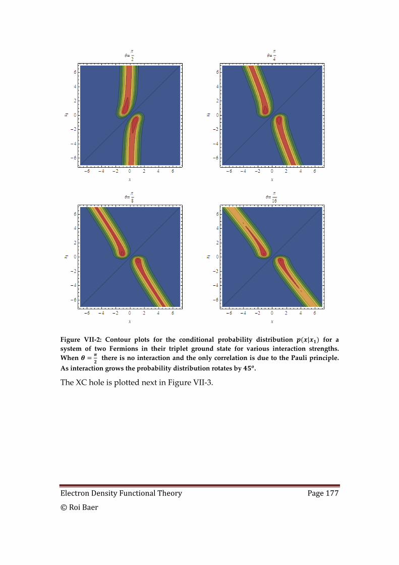
Electron Density Functional Theory Page 177
© Roi Baer
Figure VII‐2: Contour plots for the conditional probability distribution | for a system of two Fermions in their triplet ground state for various interaction strengths. When there is no interaction and the only correlation is due to the Pauli principle. As interaction grows the probability distribution rotates by .
The XC hole is plotted next in Figure VII‐3.
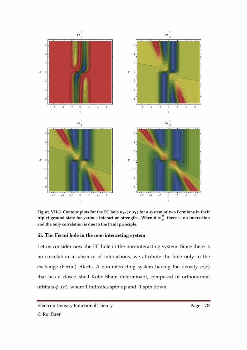
Electron Density Functional Theory Page 178
© Roi Baer
Figure VII‐3: Contour plots for the FC hole , for a system of two Fermions in their triplet ground state for various interaction strengths. When there is no interaction and the only correlation is due to the Pauli principle.
iii. The Fermi hole in the non-interacting system
Let us consider now the FC hole in the non‐interacting system. Since there is
no correlation in absence of interactions, we attribute the hole only to the
exchange (Fermi) effects. A non‐interacting system having the density
that has a closed shell Kohn‐Sham determinant, composed of orthonormal
orbitals , where 1 indicates spin up and ‐1 spin down.
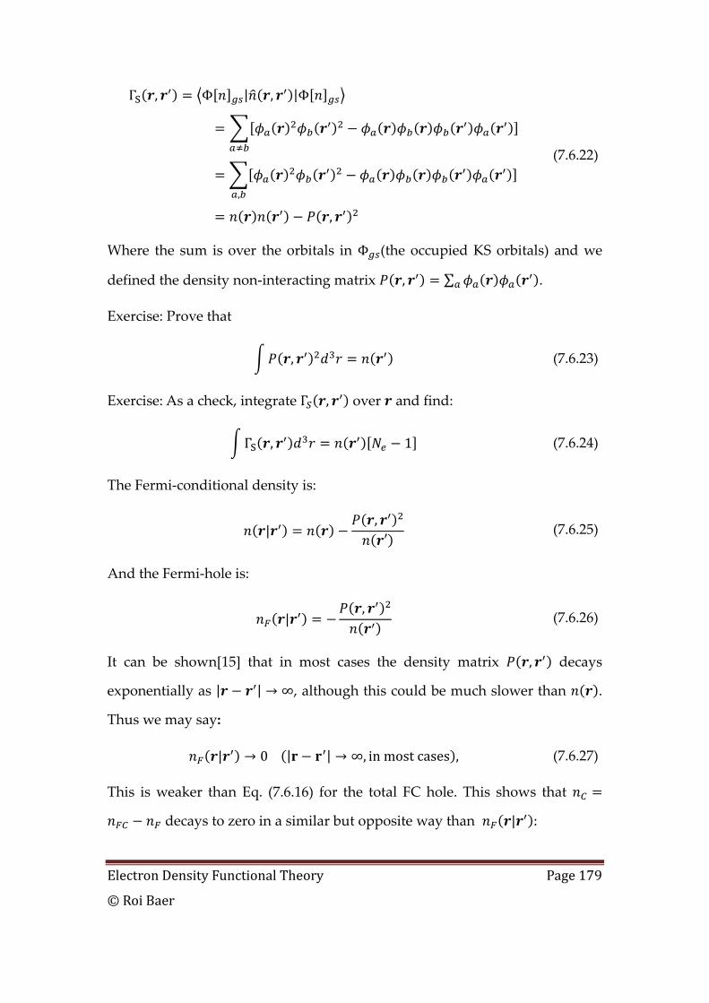
Electron Density Functional Theory Page 179
© Roi Baer
ΓS , Φ | , |Φ
,
,
(7.6.22)
Where the sum is over the orbitals in Φ (the occupied KS orbitals) and we
defined the density non‐interacting matrix , ∑ .
Exercise: Prove that
, (7.6.23)
Exercise: As a check, integrate Γ , over and find:
ΓS , 1 (7.6.24)
The Fermi‐conditional density is:
|,
(7.6.25)
And the Fermi‐hole is:
|,
(7.6.26)
It can be shown[15] that in most cases the density matrix , decays
exponentially as | | ∞, although this could be much slower than .
Thus we may say:
| 0 | | ∞, in most cases , (7.6.27)
This is weaker than Eq. (7.6.16) for the total FC hole. This shows that
decays to zero in a similar but opposite way than | :

Electron Density Functional Theory Page 180
© Roi Baer
| | | | ∞, in most cases , (7.6.28)
Based on Eq. (7.6.23) the Fermi hole carries all the charge of the FC hole:
| 1 (7.6.29)
This allows one to say that it is the Fermi or “exchange”‐hole in the non‐
interacting system that “carries the charge” of the exchange correlation‐hole
in the interacting system. Once the interacting system has been mapped onto
the non‐interacting system the Fermi‐hole is easily calculated. This can be
used to define the Coulomb hole by:
| | | (7.6.30)
It has no total charge:
| 0 (7.6.31)
The interaction energy can be written now as:
12
|| | (7.6.32)
Exercise: Compute the Fermi‐hole function of the homogeneous electron gas
Solution: We already determined the density matrix (see Eq. (5.2.24))
3 (7.6.33)
where | | and . The x‐hole is of course independent
of :
; 9 (7.6.34)
Plotting shows the form of the HEG x‐hole function:
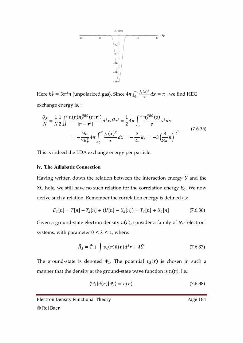
Electron Density Functional Theory Page 181
© Roi Baer
Here 3 (unpolarized gas). Since 4 , we find HEG
exchange energy is, :
1 12
;| |
12 4
92
432 3
38
/
(7.6.35)
This is indeed the LDA exchange energy per particle.
iv. The Adiabatic Connection
Having written down the relation between the interaction energy and the
XC hole, we still have no such relation for the correlation energy . We now
derive such a relation. Remember the correlation energy is defined as:
(7.6.36)
Given a ground‐state electron density , consider a family of ‐ʺelectronʺ
systems, with parameter 0 1, where:
(7.6.37)
The ground‐state is denoted Ψ . The potential is chosen in such a
manner that the density at the ground‐state wave function is , i.e.:
Ψ | |Ψ (7.6.38)
-20 -10 10 20s kF
-1.0
-0.8
-0.6
-0.4
-0.2
rX HsLên

Electron Density Functional Theory Page 182
© Roi Baer
This is a generalization of the idea by Kohn and Sham, that the interacting
electron system is mapped onto a non‐interacting electron system with the
same density. Except that now we map our system to a system of electrons
with interaction . When 0 we have the non‐interacting system and
is the Kohn‐Sham potential and we have:
(7.6.39)
where is the kinetic energy of non‐interacting electrons. When 1 we
have the fully interacting system and is the actual external
potential on the electron system and the energy is:
(7.6.40)
We can also define the obvious quantities:
(7.6.41)
From Eq. (7.6.36):
,
(7.6.42)
With:
, Ψ Ψ Ψ Ψ
Now, the ground‐state energy of the intermediately interacting electrons
obeys, by Hellmann‐Feynman’s theorem:
Ψ Ψ Ψ Ψ (7.6.43)
From the second equation then:

Electron Density Functional Theory Page 183
© Roi Baer
, Ψ Ψ , (7.6.44)
This expression is the differential form of the adiabatic connection. If we
integrate it with respect to from 0 to 1, we find:
Ψ Ψ . (7.6.45)
This formula is called the ʺadiabatic connectionʺ formula for the XC energy
[16]. We may write: , , , . Then , , ,
, and so
, , 0. (7.6.46)
We can rewrite , in terms of the correlation hole. Indeed, if | , is the
correlation hole for the system then using (7.6.32):
,12
|| | (7.6.47)
From which:
12
|| | (7.6.48)
And we see that the correlation energy can be obtained from the the ‐
averaged Coulomb hole, called the correlation hole (since it is associated with
the correlation energy):
| | (7.6.49)
Note that because , 0, we have also:
Electron Density Functional Theory Page 184
© Roi Baer
| 0 (7.6.50)
It is interesting that the correlation energy, like to Coulomb energy, can be
represented as a Coulomb interaction of the density and a hole as in Eq.
(7.6.48). Note however that the relevant hole as a coupling‐constant ( )
averaged correlation hole and not the Coulomb hole itself.
Let us discuss one of the important consequences of Eq. (7.6.50) i.e. that the
total charge of the correlation hole is zero for localized charge systems. If we
rewrite the correlation energy as:
12
|| | (7.6.51)
We see that the correlation energy can be written as
(7.6.52)
where:
2|
| | (7.6.53)
(Note that this is just a suggestion since adding to any function Δ
for which Δ 0 will give the same correlation energy).
Because for a fix | is an oveall neutral charge density in space its
“Coulombic potential” is expected to decay relatively fast for r’(faster
than 1/ ).
H. Derivative Discontinuity in the exchange
correlation potential functional
Electron Density Functional Theory Page 185
© Roi Baer
VIII. Approximate correlation energy
functionals
While the correlation energy in atoms and molecules is only a small fraction
of the total electronic energy, it is found that it is in fact a very large
percentage when one computes energy differences, such as energy of
atomization (i.e. the difference between the energy of the atomic constituents
to the energy of the molecule) or relative energies of different conformations,
as those determining the shape of the Born‐Oppenheimer potential surface. In
essence, the exchange correlation energy is the chemical bonding energy. It is
therefore crucial to model this energy accurately. We describe below some of
the basic approximations for density functional theory.
A. The local density approximation (LDA)
The mapping of the interacting electron system onto the non‐interacting
system, encapsulated in Eq. XX, is of formal interest only, unless we devise a
way to approximate the correlation potential. One way is to consider the
correlation energy per electron in the homogeneous electron gas of
density . This energy can be computed with relatively high precision using
Monte Carlo methods. Under this approximation we can write the correlation
energy as . However, this does not yield in practice good
enough results and is thus seldom used. A more successful ways was devised
by Kohn and Sham. They considered both the exchange and correlation per
an electron in the homogeneous gas, . In this case the correlation energy
comes out:
(8.1.1)
Electron Density Functional Theory Page 186
© Roi Baer
This approximation is called the local density approximation (LDA)[17]. The
functional . It leads to the following LDA approximation for the
energy functional:
(8.1.2)
The minimization of this functional, by the Kohn‐Sham approach leads to the
LDA approximation of DFT. This approach is highly successful and is
considered in DFT as the basis for most of the developments of other
functionals.
Note however that in LDA the correlation energy is extremely awkward
looking because of the term – . The presence of this term has detrimental
effects which harm some of the predictions of DFT.
i. The exchange energy per electron in the HEG
In section XXX we discussed in some detail the Hartree‐Fock theory of the
homogeneous electron gas. We defined a Jellium as a smeared positive
background of Volume at density together with electrons. We
showed that the Jellium self energy, the Jellium‐electron attraction energy and
the electron Hartree energy all cancel exactly in the HEG. Thus, the energy
per particle is given by:
(8.1.3)
We already calculate exchange energy, using a Hartree‐Fock treatment of the
HEG and we saw that / (see Eq. (5.2.32)) with /
.
In terms of the Wigner‐Sietz radius, which is a dimensionless quantity given
by:
Electron Density Functional Theory Page 187
© Roi Baer
34
/
(8.1.4)
is the radius of a Jellium sphere containing the charge of an electron. Thus:
243256
/ 0.45817 (8.1.5)
If we have a way of computing and , we can then find from
Eq. (8.1.3). We can then also compute from Eqs. (8.1.5).
ii. Correlation energy of the HEG: the high density limit
The calculation of can presently be done analytically in two limits. One is
the high density limit 0 where the kinetic energy dominates and the
Coulomb interaction can be treated as a perturbation. In this limit the kinetic
energy is that of non‐interacting particles. Thus in the perturbative approach
one can take ∑ . The unperturbed wave function is the Slater
wave functional wave function Ψ composed of the plane wave orbitals √
with taking the lowest momentum vectors . The energy of the
unperturbed state is ∑ . The first order contribution of the the e‐e
Coulomb repulsions is Ψ Ψ . This quantity is equal to the direct and
exchange contribution (see Eq. (4.1.12)). The direct part is nullified by the
other electrostatic interactions, so the 1st order contribution is essentially the
exchange energy of the HEG which we already included (see Eq. (8.1.3).
Thus to continue and determine the interaction energy beyond exchange, i.e.
the correlation energy, we must move to at least second order perturbation
theory. When one does this, one finds that the usual second order
perturbation theory yields infinite terms. These are associated with low wave
length excitations where a pair of electrons having the momentum statse|
Electron Density Functional Theory Page 188
© Roi Baer
and | , are excited by the Coulomb interaction 4 / to states |
and | (such that and ). One can show
that for small this process gives a term proportional to ln in the expression
for the 2nd order perturbation energy. This term is singular at low . A method
of performing perturbation theory which is non‐singular and goes beyond
second order, was devised in 1957[18]. This theory is essentially exact at the
high density limit and leads to the following relation:
ln (8.1.6)
Where is the Wigner‐Seitz radius, namely is the radius of a
sphere in the Jelium which scoops an amount of charge equal to 1 , where is
the elecmentary quantum of charge (the electron charge). 0.0311 and
0.048 0.001 . Later work refined these constants: 0.031091
and 0.046644 .
Exercise VIII‐1
Using Eq. (1.9.43) and the Hellman‐Feynman theorem prove that
3 4 3 4 (8.1.7)
Hints:
(a) Show that where and are, respectively, the total
electronic repulsion energy per electron and the Hartree energy per electron.
(b) From the the fact that / show that the last equality is correct.
Electron Density Functional Theory Page 189
© Roi Baer
iii. Correlation energy of the HEG: the low density limit and the Wigner
crystal
The second limit is that of low density, where the electrons form a crystal. We
give the development of this limit, originally proposed by Wigner[19] when
he devised a theory for the electron density in metallic sodium.
Wigner assumed that at low energy the homogeneous electron gas forms a
crystal. Now that may sound strange: how can the density be uniform and at
the same time the electrons form a crystal? Thanks to Quantum Mechanics
this is actually not a contradiction, as the following example shows.
Exercise: Show that for 2 particle in a 3D box of volume with periodic
boundary conditions, if the Hamiltonian is:
2 2 (8.1.8)
Then
1) The eigenstates have a homogeneous 1‐particle density
2) The pair correlation function has structure. ( , ||
,
In the low density regime the electron kinetic energy (per electron) can be
neglected since, as seen in XXX it is proportional to while the repulsion
energy between the electrons per electron is proportional to . At lkow
density the Pauli exclusion priniciple is non‐operative, since electrons do not
overlap. Thus the quantum nature of the electron is gone at this limit and we
can think of the electron as a classical particle that localizes. This is because
non‐localization of particles in quantum mechanics arises only from their
need to reduce kinetic energy. The electrons will arrange themselves in the
lowest energy state by forming a close packed crystal. Each electron is then as
far as possible from each other electron, while still filling 3D space with
Electron Density Functional Theory Page 190
© Roi Baer
average density n . Let us calculate the energy of such a crystal. Consider one
of the electrons in the crystal. We imagine it together with a cell containing 1
unit of positive charge. This cell shape depends on the crystal symmetry.
Following Wigner, we neglect the crystal structure and assume each electron
is surrounded by a sphere of positive charge completely neutralizing it. Our
approximation then neglects the volume of the space between the spheres.
The radius of the sphere is and it is filled with smeared positive charge and
with one negative charged point‐electron at its center. The spheres do not
interact since they are neutral and have no electric moments.
The total energy per electron is the energy to assemble the Jellium
sphere and the energy needed to bring the electron from infinity into
the center of the sphere.
Let be the energy to assemble a sphere of charge density and radius
. Suppose we now enlarge it by adding a shell of radius . The electric
potential at distance outside the sphere is / where is the
charge in the sphere. The charge in the shell is 4 and bringing it
from infinity, where the potential is zero to its place on top of the existing
sphere involves the energy . Thus, by integration
from 0 to , we find: . And so at :
351
(8.1.9)
Next, we want to calculate the energy to bring an electron from infinity to the
center of the sphere. This will be done in two stages, first bringing the electron
from infinity to the rim of the sphere, a distance from its center and then
from the rim to the center. Accordingly write . The first part
Electron Density Functional Theory Page 191
© Roi Baer
is easy since we already know the potential, and it is negative since energy is
released by this process, so:
1 (8.1.10)
Inside the sphere, at a distance from the center there exists an electric field
due to the Jellium, which according to Gauss’ is . This force
is a Harmonic force, with force constant . The work to move
an electron in this field to the center is: . The
energy for the second stage is therefore and the total energy per
electron in the crystal is:
910
1 (8.1.11)
This then is the exchange‐correlation energy for low density. We neglected the
volume between the spheres. The exchange energy we already know from
(8.1.5), is . . Thus, Wignerʹs approximation for the
correlation energy in the low density limit is:
0.44183, ∞ (8.1.12)
Wigner also considered the correction due to the finite kinetic energy when
is finite. Since we saw that the electron inside the spherical Jellium drop is a
Harmonic potential, one can reduce the correlation energy by the 3D
Harmonic zero‐point potential, / . The correlation energy is then:
0.44183 32 / , ∞ (8.1.13)

Electron Density Functional Theory Page 192
© Roi Baer
iv. Monte-Carlo determination of the correlation energy for the HEG
Between these high and low limits there is no analytical theory, in general and
a numerical computation can be made based on quantum Monte Carlo
methods. The results of the calculation are then fitted to an analytical form
which respects the limits
v. The polarized HEG; local spin-density approximation (LSDA)
Up to now we have assumed that the electron gas is unpolarized, i.e. the total
z component of spin Sz per electron is zero. However, Sz is a good quantum
number and it can vary continuously from to . The extreme case is the
fully polarized case. In general one may define the density of spin‐up electron
and that of spin down . Then:
(8.1.14)
For a fully polarized gas 1 and the difference is first of all in the Fermi
energy. For the HEG, since every momentum state can populate only one
electron, we find by a similar analysis as in the unpolarized case:
1 /
2 1 /
35
(8.1.15)
The total kinetic energy us the sum of up and down contributions:
, which is evaluated to be using the expressions for
we obtain
Electron Density Functional Theory Page 193
© Roi Baer
35
1 / 1 /
2 (8.1.16)
As for exchange energy, since exchange interaction occurs only between like
spins, we XXXXX
vi. Successes and failures of LSDA
vii. Plausible reasons for the success of LSDA
One of the uses of Eq. (7.6.48) expression is to explain the success of a simple
theory such as LDA[20]. TO see this, let us expand the XC hole in terms of
moments around :
, ; , (8.1.17)
where: sin cos , sin sin , cos and
; , , sin (8.1.18)
Then consider the XC energy, it can be written as:
12
,
12√4
,
(8.1.19)
Were:
, , (8.1.20)
And:
Electron Density Functional Theory Page 194
© Roi Baer
√4 , 1 (8.1.21)
Thus, only the 00 moment of the dependent XC holes enters the expression.
Therefore, in a sense the angular shape of the average XC hole gets averaged
over and only the radial dependence affects the XC energy. This is used to
explain some of the success of LDA.
We see that the XC anisotropy of the XC hole around r is averaged over. Only
this average enters the XC energy formula. In LDA we use the homogeneous
electron gas to compute the HEG. Of course this leads to an isotropic XC hole.
Yet, since only the spherical average of the hole enters into the XC energy, this
drastic approximation gives a reasonably good XC energy.
Exercise: Calculate the spherically averaged X‐hole for a 1‐electron system (H
atom for example)
Solution: The orbital is , the density is and the DM is
, thus:
; (8.1.22)
The hole is independent of the reference point .
One of the important results shown below is that only the spherically
averaged hole enters the XC energy. Thus we only need the spherically
averaged hole:
;14 ; Ω (8.1.23)
Which becomes:
, ;14 Ω (8.1.24)
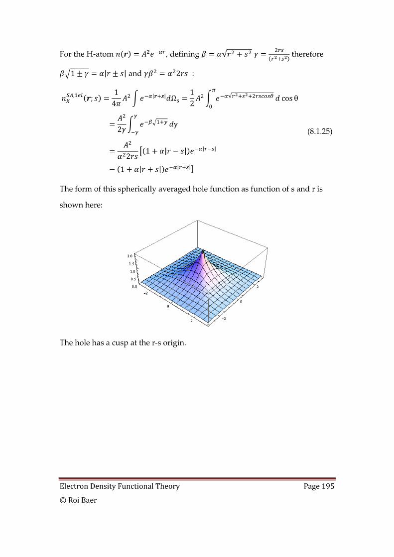
Electron Density Functional Theory Page 195
© Roi Baer
For the H‐atom , defining √ therefore
1 | | and 2 :
, ;14
| | Ω12
√ cos θ
2 y
2 1 | | | |
1 | | | |
(8.1.25)
The form of this spherically averaged hole function as function of s and r is
shown here:
The hole has a cusp at the r‐s origin.
Electron Density Functional Theory Page 196
© Roi Baer
B. Semilocal functionals and the generalized
gradient approximation
IX. Generalized Kohn-Sham approaches
A. The generalized Kohn-Sham framework
The Kohn‐Sham approach is based on pure density functionals for the
exchange correlation energy. This approach is based on the Hohenberg‐Kohn
universal density functional is written as:
(9.1.1)
We noted one problem with is that it is not defined for all densities. This
problem can be cured by the Levy‐Lieb procedure, where the is replaced
by a functional based on a constrained minimum principle:
min Ψ Ψ (9.1.2)
Similarly, for the non‐interacting system, one finds:
min Φ Φ min Φ (9.1.3)
Where here the search is over all determinants. Here we defined here a new
determinantal functional Φ] with the intent of generalizing the KS
approach, as we do now. Using the minimizing determinant Φ , the Kohn‐
Sham correlation energy:
(9.1.4)
Is written using ΦS ΦS and ΦS ΦS .
Since a Slater wave function is given in terms of orthonormal one‐electron
orbitals , it is best to view as a functional of the orbitals and we write
. We can now generalize and demand that not be just the kinetic

Electron Density Functional Theory Page 197
© Roi Baer
energy but a more general functional of the Slater wave function. We denote
the functional derivative of as follows:
Φ (9.1.5)
Where is some convenient operator.
We now define the energy functional for a given potential and
determinant Φ:
, Φ Φ Φ (9.1.6)
Where:
Φ Φ| |Φ (9.1.7)
We then minimize with respect to the orbitals of
Φ, keeping them normalized. This constrained minimization results in the
orbital equations:
. (9.1.8)
Furthermore, let us define the density functional resulting from
minimizing with constrained of a given density:
min Φ . (9.1.9)
From this we further define the density functional :
(9.1.10)
In actual implementations the functional must of course be approximated.
Now we put all ingredients together. The HK DFT energy is developed as a
train of equalities as follows:
Electron Density Functional Theory Page 198
© Roi Baer
min
min
min min Φ
min Φ Φ Φ
(9.1.11)
In the last step we changed the order of the minimum procedure, assuming
this is OK. Note that the final procedure is minimization with respect to
orbitals instead of to density. The minimization, under normality of the
orbitals from which the Slater wave function is built is gives the
generalized Kohn‐Sham equation:
(9.1.12)
Where:
(9.1.13)
If we write:
(9.1.14)
we find that the orbitals also obey equations (9.1.8). Thus, the density
obtained from the orbitals of the GKS procedure is the minimizing density of
the following density functional
min (9.1.15)
The strength of the GKS scheme is that it incorporates explicit orbital
functionals. This greatly enlarges the scope of approximations for DFT.
Electron Density Functional Theory Page 199
© Roi Baer
B. Kohn-Sham from generalized KS
By choosing: Φ Φ Φ one immediately obtained the usual KS
theory, with .
C. The Hybrid functional of Becke
Let us return to the adiabatic connection formula Eq. (7.6.45):
Ψ Ψ (9.2.1)
Becke [21], suggested the following trapezoidal approximation for the
integral:
Ψ Ψ Ψ Ψ Ψ Ψ
2 (9.2.2)
Leading to the Becke’s Half & Half approximation:
12
12
12
12 (9.2.3)
The function is next approximated as a local density functional:
(9.2.4)
Where . the interaction energy per electron in a
homogeneous electron gas is . This function can be computed using the
Quantum Monte‐Carlo results concerning the XC energy.
Becke showed that this half and half theory gives a big improvement over
LDA and in some cases also over GGA functionals. This is because he has
found a way to approximate Hartree‐Fock theory and LDA.
The Becke Half & Half orbital (BH&H) was the first example of a hybrid
theory, a theory which is a mixture of a Hartree‐Fock functional of orbitals
Electron Density Functional Theory Page 200
© Roi Baer
and a DFT functional of density. Becke eventually wrote down a functional
which contains 3 parameters [22]:
, … ,
XCLSDA
XLSDA
XB
XLSDA
CPW
CLSDA
(9.2.5)
We see that the B3LYP functional starts from a LSDA functional and adds to it
3 corrections. One is a fraction of the explicit orbital exchange correction
XLSDA then a correction X
BXLSDA to the LSDA exchange
given by a GGA type functional called Becke88 [23] and finally a GGA
correction for the correlation energy, given by the PW91 functional [24]. The
values of the 3 parameters 0.20, 0.72 and 0.81 were found by
optimizing the performance of the functional for 56 atomization energies, 42
ionization potentials (calculated by Δ method) and 8 proton affinities.
D.
E. Long-Range self-repulsion and lack of
derivative discontinuity
F. Range separated hybrids
G. Orbital functionals and optimized effective
potentials
H. Approximate correlation functionals and the
Born-Oppenheimer force on nuclei
The Kohn‐Sham density functional theory method (KS‐DFT), when applied
for electrons of molecules makes sense only for frozen nuclei, because the
external potential in DFT is assumed time‐independent. However, the nuclei
Electron Density Functional Theory Page 201
© Roi Baer
in molecules are not in general motionless. How do we KS‐DFT a useful
approach for molecules? Here we use the Born‐Oppneheimer approximation,
which allows us to divide the electron‐nuclear problem into 2 stages: first
computing the electronic energy for each nuclear configuration
and then combining it with the nuclear repulsion energy to
obtain an effective potential for the motion of the nuclei. The nuclear‐electron
potential is given by:
, | | (9.3.1)
In order to compute the electronic energy we first write down the functional:
, (9.3.2)
We then minimize it under the constraint for the number of electrons
. This gives a minimizing density and we have:
, (9.3.3)
Since in exact DFT is the exact electronic energy, we are assured that:
, (9.3.4)
Since this relation is true for the electronic Hamiltonian (as can be seen from
Hellman‐Feynamn theorem).
However, what happens when we use an approximation for , as done in
all applications of KSDFT? Does this relation still hold? We now show that
indeed it does.
The density is determined by:
Electron Density Functional Theory Page 202
© Roi Baer
(9.3.5)
The electronic force on the nuclei is given by:
,
(9.3.6)
The second integral is zero because:
0 (9.3.7)
Thus we find that the relation:
, (9.3.8)
still holds. Even if the approximate XC functional does not yield the exact
density, the formal relation between the force and the density is still valid.
Electron Density Functional Theory Page 203
© Roi Baer
X. More on the DFT correlation energy
A. Approximations to EX are approximation to EC
In Kohn‐Sham DFT the ground state energy of a system of electrons having
the particle‐density is written as a sum of density functionals[17]:
(10.1.1)
Here, is the kinetic energy of a system of non‐interacting fermions having
the same mass and ground‐state density as the electrons, the external
potential exerted on the electrons, | | is the so‐called
Hartree energy of the system and is the XC energy functional. The
explicit form of the latter functional is formally known but practically
inaccessible to computation. The basic challenge in DFT is to develop an
efficacious approximation to the XC energy functional.
The most widely used functionals of DFT fall into two broad categories.
Semilocal functionals which are based locally on the density the orbitals of the
non‐interacting system or on their derivatives, such as the local density
approximation (LDA), generalized gradients approximation (GGA) and Meta‐
GGAs [23, 25] The second category includes non‐local functionals such as the
widely used B3LYP[22]. Recently a new brand of hybrid functionals was
developed, designed to remove the long range self‐interaction in DFT[26‐28].
For a given density one can use the wave function Ψ of the non‐interacting
system and define the “exact exchange energy“ ΨS| |ΨS ,
where ∑ is the repulsion energy operator. The functional defined
by is called the correlation energy functional. Kohn
Electron Density Functional Theory Page 204
© Roi Baer
and Sham[17] recognized that in practical calculations it is beneficial to
approximate the exchange energy than to use its exact form. Indeed it was
found that the errors introduced into by using simple approximations to
are partially cancelled by the approximate treatment of the exchange
energy. This error cancellation is the one of the major reasons for success of
DFT. Since is actually known exactly and easy to calculate, it is evident that
using an approximate exchange functional in place of the exact is a
way to correct the approximate correlation energy. For example, the
correlation energy functional in the LDA is NOT the LDA of the correlation
energy , but instead:
(10.1.2)
This view emphasizes the fact that LDA of local exchange is a way of
correcting the correlation energy for inhomogeneous systems. Similar
expressions are to be used in more advanced functionals (GGA etc). Any
correction to for example, using a GGA type expression
, | | should be viewed as an essentially correlation
correction.
This way of thinking leads naturally to hybrid functionals. A hybrid
functional is a further improvement of LDA (or GGA) obtained simply by
multiplying the correction in (10.1.2) by a factor :
, (10.1.3)
Or, based on BLYP, one of the GGA functionals we can write:
, , | | , | | (10.1.4)
Electron Density Functional Theory Page 205
© Roi Baer
Becke [22] found by a series of calculations on many molecules that the
“natural” assumption 1 is not optimal and should be somewhat smaller,
around 0.8. This lead to development of the extremely successful B3LYP
functional. However, experience has shown that some systems require lower
values of while others strive for higher values. An example is reaction
barriers where lower values of (around 0.5‐0.7) were needed. There is
presently no general systematic way to set the value of .
The hybrid DFT approaches are well established electronic structure methods
however in the past few years it has become increasingly clear that several
types of calculations, for example, polarizability, electron transfer excitations,
Rydberg states and charge allocation in weakly coupled systems are often not
well described by the above DFT/TDDFT methods[29‐31]. This deficiency,
which is not cured by the Becke approach to hybrid functionals, was
attributed to spurious self interaction[32] and missing derivative
discontinuities[33] ‐ two pervasive problems in density functional theory
(DFT) that are intimately related.[34, 35]
One way to mitigate the spurious self interaction and to retain a good
treatment of correlation is to deploy a range‐separated hybrid functional[26‐
28, 34, 36] In this approach, the exchange term in the Kohn Sham energy
functional is split into long‐range and short‐range terms, e.g., via
c . The short‐range exchange is represented by a
local potential derived from a Semilocal functional. The long‐range part is
treated via an “explicit” or “exact” exchange term. If one assumes that an
appropriate choice for γ is system independent, its value can be optimized
using a molecular training set for optimizing its value. Such semi‐empirical
approaches, typically with γ in the range of 0.3‐0.5 a0‐1, were shown to
Electron Density Functional Theory Page 206
© Roi Baer
achieve impressive results for the ground state properties of some classes of
systems.[27, 37, 38] Furthermore, it was demonstrated on the benchmark
model of Dreuw and Head‐Gordon[39] ‐ the C2H4…C2F4 dimer at large
molecular distances ‐ that the range‐separated hybrid corrects the principal
deficiencies of the charge transfer excitation prediction of TDDFT.[38, 40]
One of the drawbacks of the semilocal DFT and Becke schemes is that the
correlation energy of Eqs. (10.1.3) ‐ (10.1.4) is much too nonlocal due to the
presence of the nonlocal exchange . This is unbalanced in view of the
presence of in the total energy. This is the root cause of long‐range “self
repulsion” which exists in all these functionals. A way to improve the
situation is to include in the exchange functional a non‐local long‐range
exchange, which leads to the following form for the correlation[26, 27, 41]:
, , | |
, | | , , | |
,
(10.1.5)
The functional , is the exchange energy of a system of particles at density
mutually interacting through the repulsive potential where is
a parameter:
,12
| , | . (10.1.6)
, is a semilocal density approximation to the complementary
interaction . The idea behind this appealing
approach is to eliminate in the correlation functional the long range
dependence on the density. is treated as a universal parameter determined
by fitting the DFT predictions based on Eq. (10.1.5) to a large database of
Electron Density Functional Theory Page 207
© Roi Baer
experimental data. This forms the basis of several recent semi‐empirical
approaches all of which use a universal long‐range parameter determined
by semiempirical fitting to known experimental and sometimes high quality
ab‐initio results [26‐28, 34, 36‐38]. These approaches have been quite
successful for a broad variety of molecules, sometimes beyond the types used
in the fitting procedures.
The approach of a universal exchange functional with complementary
semilocal functionals cannot however claim universality. In some systems the
exact value of is critical and no semilocal DFT method can correct for it. We
show examples below. An alternative view was developed in ref. [28], which
provides a theory for the long‐range parameter based on the adiabatic
connection theorem, from which the following exact expression for the
correlation energy can be deduced:
Ψ Ψ ΨS ΨS (10.1.7)
Where ∑ . In ref. [28] arguments were given for the
existence of a parameter for which Eq. (10.1.7) holds for practically all
densities. This equation describes the correlation energy as a difference
between potential energies of interaction in the interacting and in the non‐
interacting systems. Unlike the standard definition of correlation energy as
Ψ Ψ ΨS ΨS Ψ Ψ ΨS ΨS , the there are no
explicit contributions of kinetic energy differences in Eq. (10.1.7). These are
absorbed by the interaction screening parameter . In principle all quantities
in this equation, including , are density‐dependent. We stress that the
difference between this exact theory and the usual exposition of RSHs is that
the latter do not derive (or even strive to derive) an exact expression for the
correlation energy. Eq. (10.1.7) can be applied to the HEG and the exact value
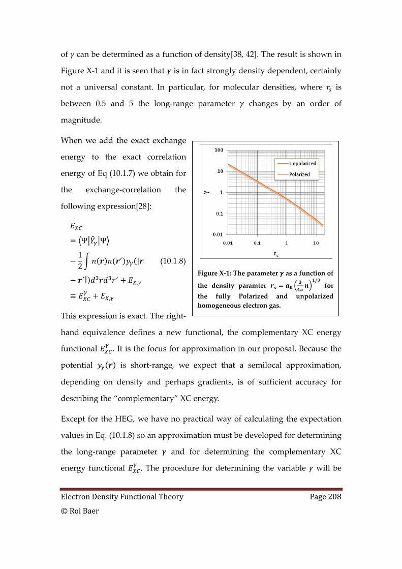
Electron Density Functional Theory Page 208
© Roi Baer
of can be determined as a function of density[38, 42]. The result is shown in
Figure X‐1 and it is seen that is in fact strongly density dependent, certainly
not a universal constant. In particular, for molecular densities, where is
between 0.5 and 5 the long‐range parameter changes by an order of
magnitude.
When we add the exact exchange
energy to the exact correlation
energy of Eq (10.1.7) we obtain for
the exchange‐correlation the
following expression[28]:
Ψ Ψ
12
|
| ,
,
(10.1.8)
This expression is exact. The right‐
hand equivalence defines a new functional, the complementary XC energy
functional . It is the focus for approximation in our proposal. Because the
potential is short‐range, we expect that a semilocal approximation,
depending on density and perhaps gradients, is of sufficient accuracy for
describing the “complementary” XC energy.
Except for the HEG, we have no practical way of calculating the expectation
values in Eq. (10.1.8) so an approximation must be developed for determining
the long‐range parameter and for determining the complementary XC
energy functional . The procedure for determining the variable will be
Figure X‐1: The parameter as a function of
the density paramter / for
the fully Polarized and unpolarized homogeneous electron gas.
Electron Density Functional Theory Page 209
© Roi Baer
called below “long‐range parameter tuning”. We now show some preliminary
results which demonstrate the fact that one cannot rely on a universal long‐
range parameter .
B. The necessity of long-range parameter tuning
The requirement for a system‐dependent parameter is not just a theory it
comes up in practical calculations. Here we give two examples of unpublished
results, one in DFT and one in TDDFT.
i. The symmetric radical cation
In DFT, a clear example of this issue is seen in the symmetric radical cation
systems of the type , where is any molecule or atom. Specific
examples are H,He and Ne. It is known that for these systems a semilocal
or even nonlocal (B3LYP) DFT gives qualitatively spurious potential surfaces
and the big issue is self‐repulsion[1, 43].Yet, even with a standard ‐functional
the results are not satisfactory. Take for example the bond dissociation energy
(BDE). This can be estimated in two ways. The first is the atomization energy.
The second is the depth of the molecular well relative to the asymptote of the
potential surface. From both numbers we subtract the zero‐point vibrational
energy to get the BDE. We can see in Table 1 that the BDE of R=He and Ne
based on atomization energy using a semi‐empirical 0.5 (denoted
BNL functional[38]) gives BDE around 1.5‐2 times the experimental value!
While in the asymptotic method the calculated BDE is too small by 15%. Such
discrepancies cannot be waived by a better semilocal functional. They reflect
an inherent imbalance between short and long range exchange inflected by a
wrong long‐range parameter . Indeed, by tuning the long‐range parameter in
the following way we obtain a value which is specific for each system. The
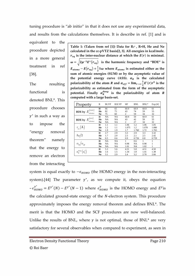
Electron Density Functional Theory Page 210
© Roi Baer
tuning procedure is “ab initio” in that it does not use any experimental data,
and results from the calculations themselves. It is describe in ref. [1] and is
equivalent to the
procedure depicted
in a more general
treatment in ref
[38].
The resulting
functional is
denoted BNL*. This
procedure chooses
in such a way as
to impose the
“energy removal
theorem” namely
that the energy to
remove an electron
from the interacting
system is equal exactly to (the HOMO energy in the non‐interacting
system).[44] The parameter , as we compute it, obeys the equation
– 1 where is the HOMO energy and is
the calculated ground‐state energy of the ‐electron system. This procedure
approximately imposes the energy removal theorem and defines BNL*. The
merit is that the HOMO and the SCF procedures are now well‐balanced.
Unlike the results of BNL, where is not optimal, those of BNL* are very
satisfactory for several observables when compared to experiment, as seen in
Table 1: (Taken from ref [1]) Data for R2+ , R=H, He and Ne calculated in the cc‐pVTZ basis[2, 3]. All energies in kcal/mole. is the inter‐nuclear distance at which the is minimal.
is the harmonic frequency and “BDE” is
where is estimated either as the sum of atomic energies (SUM) or by the asymptotic value of the potential energy curve (ASS). is the calculated polarizability of the atom and is the polarizability as estimated from the form of the asymptotic potential. Finally is the polarizability of atom computed with a large basis‐set.
Property R BLYP B3LYP HF BNL BNL* Exp.[4]
BDE by ( )sum
atomsE
H 66 65 60.9 60.9 60.9 61 He 82 75 43 74 59 55 Ne 75 60 2 59 34 32
BDE by ( )ass
atomsE
H NA NA 60.9 50 60.9 61 He NA NA 43 42 59 55 Ne NA NA 2 27 34 32
( )Åeqr
H 1.1 1.1 1.06 1.2 1.06 1.05 He 1.2 1.1 1.075 1.2 1.078 1.080 Ne 1.9 1.9 1.7 1.760 1.72 1.765
2ω H 2.7 2.9 3.3 2.9 3.3 3.32 He 1.7 2.0 2.5 2.1 2.5 2.42 Ne 0.5 0.6 0.9 0.726 0.8 0.729
R effα α
H NA NA 1 0.6 1 1 He NA NA 0.98 NA 0.98 1 Ne NA NA 1.01 NA 1.02 1
( )30daugRa a H 5.3 5.6 4.51 5.8 4.51 4.50
He 1.6 1.5 1.34 1.8 1.41 1.38 Ne 3.1 2.9 2.4 3.2 2.70 2.66
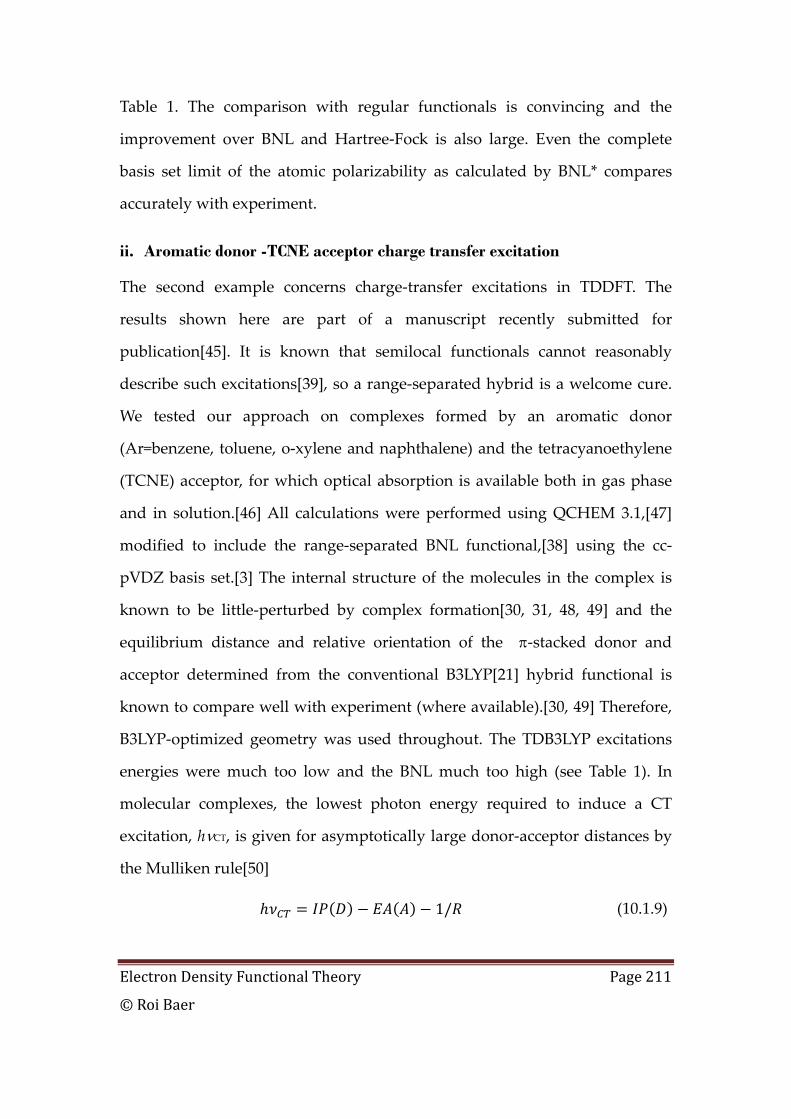
Electron Density Functional Theory Page 211
© Roi Baer
Table 1. The comparison with regular functionals is convincing and the
improvement over BNL and Hartree‐Fock is also large. Even the complete
basis set limit of the atomic polarizability as calculated by BNL* compares
accurately with experiment.
ii. Aromatic donor -TCNE acceptor charge transfer excitation
The second example concerns charge‐transfer excitations in TDDFT. The
results shown here are part of a manuscript recently submitted for
publication[45]. It is known that semilocal functionals cannot reasonably
describe such excitations[39], so a range‐separated hybrid is a welcome cure.
We tested our approach on complexes formed by an aromatic donor
(Ar=benzene, toluene, o‐xylene and naphthalene) and the tetracyanoethylene
(TCNE) acceptor, for which optical absorption is available both in gas phase
and in solution.[46] All calculations were performed using QCHEM 3.1,[47]
modified to include the range‐separated BNL functional,[38] using the cc‐
pVDZ basis set.[3] The internal structure of the molecules in the complex is
known to be little‐perturbed by complex formation[30, 31, 48, 49] and the
equilibrium distance and relative orientation of the π‐stacked donor and
acceptor determined from the conventional B3LYP[21] hybrid functional is
known to compare well with experiment (where available).[30, 49] Therefore,
B3LYP‐optimized geometry was used throughout. The TDB3LYP excitations
energies were much too low and the BNL much too high (see Table 1). In
molecular complexes, the lowest photon energy required to induce a CT
excitation, hνCT, is given for asymptotically large donor‐acceptor distances by
the Mulliken rule[50]
1/ (10.1.9)
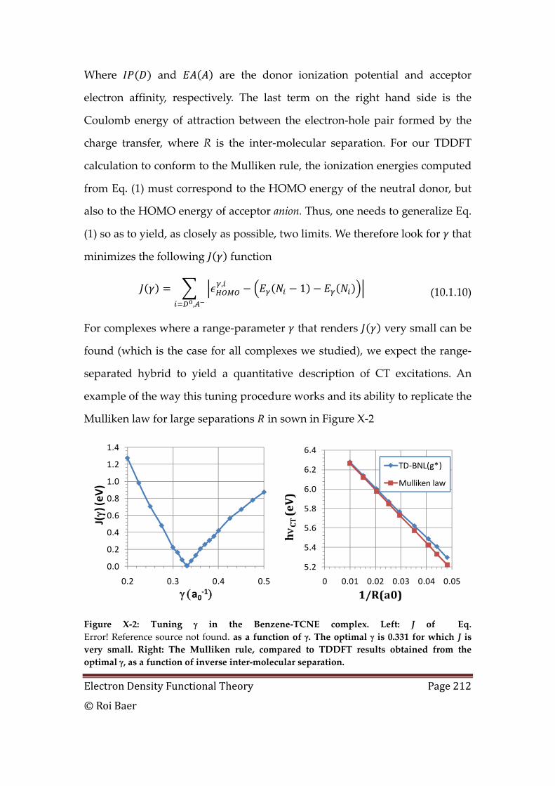
Electron Density Functional Theory Page 212
© Roi Baer
Where and are the donor ionization potential and acceptor
electron affinity, respectively. The last term on the right hand side is the
Coulomb energy of attraction between the electron‐hole pair formed by the
charge transfer, where R is the inter‐molecular separation. For our TDDFT
calculation to conform to the Mulliken rule, the ionization energies computed
from Eq. (1) must correspond to the HOMO energy of the neutral donor, but
also to the HOMO energy of acceptor anion. Thus, one needs to generalize Eq.
(1) so as to yield, as closely as possible, two limits. We therefore look for that
minimizes the following function
, 1,
(10.1.10)
For complexes where a range‐parameter that renders very small can be
found (which is the case for all complexes we studied), we expect the range‐
separated hybrid to yield a quantitative description of CT excitations. An
example of the way this tuning procedure works and its ability to replicate the
Mulliken law for large separations in sown in Figure X‐2
Figure X‐2: Tuning γ in the Benzene‐TCNE complex. Left: J of Eq. Error! Reference source not found. as a function of γ. The optimal γ is 0.331 for which J is very small. Right: The Mulliken rule, compared to TDDFT results obtained from the optimal γ, as a function of inverse inter‐molecular separation.
0.0
0.2
0.4
0.6
0.8
1.0
1.2
1.4
0.2 0.3 0.4 0.5
J(γ) (eV)
γ (a0‐1)
5.2
5.4
5.6
5.8
6.0
6.2
6.4
0 0.01 0.02 0.03 0.04 0.05
hνCT(eV)
1/R(a0)
TD‐BNL(g*)
Mulliken law
Electron Density Functional Theory Page 213
© Roi Baer
With the asymptotic behavior enforced, we expect proper balance between the
semilocal and non‐local exchange components. In Error! Reference source not
found. we compare the calculated and experimental gas‐phase results for
various Ar‐TCNE complexes. It is readily seen that the B3LYP results are
unacceptably low and predictive power is absent. Results of generalized‐
gradient (GGA) calculations (not shown) are even lower than the B3LYP ones.
With the range‐separated BNL functional,[38] excitation energies determined
with an ʺoff‐the‐shelfʺ γ value of 0.5 a0‐1 are much too high with respect to
experiment. But with γ* quantitative agreement is obtained to within ±0.2eV.
For benzene and toluene, the theoretical oscillator strengths are also in good
agreement with experiment, but are too weak for xylene and naphthalene.
This is likely a basis‐set issue, as oscillator strengths are much more sensitive
to the basis set than the excitation energies.
Electron Density Functional Theory Page 214
© Roi Baer
XI. TDDFT
A. Time-dependent Linear response theory
The linear response of
, , ,
, 0
(10.2.1)
Where the TD Hamiltonian, in the adiabatic TDDFT approximation, is:
(10.2.2)
And the TD density matrix is defined in terms of the TD orbitals:
, , , , (10.2.3)
The initial orbitals are assumed the lowest eigenstates of :
(10.2.4)
where:
, (10.2.5)
We assume that the perturbation , is weak and we will treat it as a first
order quantity. Before we do this however, let us prepare the equation for
linearization by defining:
, / , (10.2.6)
and:
Electron Density Functional Theory Page 215
© Roi Baer
, , , , ,
, , (10.2.7)
With these definitions we have:
/ ,
, / ,
(10.2.8)
From this we find:
, , , (10.2.9)
This equation is rigorously equivalent to the first equation. It is a non‐
homoegenous linear equation for the unknown .
We now make the linearization step. We neglect all quantities beyond first
order. As a first step we have:
, , , (10.2.10)
Here, the symbol “ ” means “equal to first order”. We use the definition:
(10.2.11)
An efficient method to obtain linear response of a perturbation is as follows.
Select a small parameter and solve the following time dependent equation
(using a standard propagator, such as Runge Kutta)[51]:
, ,
,
(10.2.12)
With:
Electron Density Functional Theory Page 216
© Roi Baer
, , , ,
, 2 ,
The size of must be so small that the orbital amplitudes are linear with .
The solution involves repeated applications of the Hamiltonian. This could be
considerably more efficient than the algebraic method described below,
requiring the computation of all the eigenvectors of the Hamiltonian. Of
course, for small systems with a small basis the algebraic approach may be
extremely effective thus we discuss it now.
B. Algebraic Approach to Linear response
In order to derive an algebraic approach, we need expressions for all the
linear quantities. For we find:
(10.3.1)
And:
,,
| |
, ,
, , | |
(10.3.2)
Plugging all this into Eq. (10.2.10):
Electron Density Functional Theory Page 217
© Roi Baer
,1
| | , ,
, , , | |
,
(10.3.3)
Plugging in the 1st order definitions of and we find:
, 2 , ,
, ,
,1
| | | |
,
(10.3.4)
We now take a crucial step to get rid of all the integrals and special
dependence by expanding in terms of the orthonormal complete
eigenfunction of the Hamiltonitan . Because the evolution according to
the Kohn‐Sham equation preserves orthonormality. Thus, the response
functions are orthogonal to all occupied MO’s. This allows us to write:
, (10.3.5)
We use the following index notations:
,
,
,
The operator can be turned into a 4‐index matrix:
Electron Density Functional Theory Page 218
© Roi Baer
, ,
1| | ,
| |
, ,
(10.3.6)
Using these expansions we find:
2 ,, ,
,
(10.3.7)
with: . Now multiply by and integrate over and obtain
a time‐dependent algebraic equation:
2 ,
(10.3.8)
Where:
, (10.3.9)
We can separate to two real equations by the real and imaginary parts:
Electron Density Functional Theory Page 219
© Roi Baer
2 ,
(10.3.10)
This equation can be used to get a time‐dependent response. It will be useful
for describing the response to a complicated weak pulse .
C. Frequency-domain response
Instead of viewing the response in time we can view it in frequency. This will
allow us to address questions of response to sinusoidal fields, such as laser
absorption. We Fourier‐transform the coefficients:
(10.3.11)
Note that 0 0 and so: .
Note further that and are not real anymore. In fact, because ’s are real
we now have: .
Applying a Fourier transform to the time‐dependent equations gives:
2 ,
(10.3.12)
Combining the equations we rid ourselves of and obtain an equation for
:
2 , , (10.3.13)
The number of these coupled algebraic equations is infinite. However, in any
practical application we use a finite number of states and so we have a finite
number of equations. If M is the total number of states used we then for any
Electron Density Functional Theory Page 220
© Roi Baer
given perturbation one can get an approximate response by solving one of
these two equations for . This involves solving a linear × set of
equations and obtain the response to the perturbation. We can write it in
matrix form:
. (10.3.14)
With:
2 , (10.3.15)
We now prove that as long as 0 for all possible and the matrix has
only real eigenvalues. In fact, is always positive unless there is a
degeneracy at the HOMO and the level is not full. The eigenvalue equation is:
2 , Ω (10.3.16)
where are the eigenvector components. Under the assumption we can
bring this equation to the following equivalent form:
2 , Ω (10.3.17)
Where . These new equations involve the eigenvalues of a
symmetric matrix. Thus, the eigenvalues Ω are all real. Eq. (10.3.17) is called
the Casida equations.
D. Excitation energies from the algebraic
treatment
The algebraic equation for linear response derived in Eq. (10.3.14) allows
calculation of a specific response problem. One incredible feature of this
equation is that the matrix on the left is independent of the perturbation .
We can thus analyze to get general response properties of the system,
Electron Density Functional Theory Page 221
© Roi Baer
without reference to any specific perturbation. We can define a “response
matrix”:
. (10.3.18)
Where is defined in (10.3.15)We can define right and left eigenvectors:
Ω , Ω (10.3.19)
It is easy to see from Eq. (10.3.16) that:
(10.3.20)
We choose the normalizations so that:
1 (10.3.21)
Collecting the vectors ina a matrix and the eigenvalues in a diagonal matrix
Ω we can write:
Ω (10.3.22)
And:
Ω (10.3.23)
We can now take near an eigenvalue Ω . This has an infinite response. Thus
we can then write:
Ω Ω (10.3.24)
A general technique to study the resonance is to insert an infinitesimal
imaginary part which we eventually take to zero: Ω . Then, after a
few algebraic manipulations (Ω Ω
Ω
ΩΩ
):
Electron Density Functional Theory Page 222
© Roi Baer
ΩΩ 2Ω
4Ω (10.3.25)
Thus:
lim Ω ∞
lim Ω1
4 Ω (10.3.26)
The imaginary part of the response is finite at resonances.

Electron Density Functional Theory Page 223
© Roi Baer
References
1 E. Livshits and R. Baer, J. Phys. Chem. A 112, 12789 (2008). 2 D. E. Woon and T. H. Dunning, J. Chem. Phys. 100, 2975 (1994); R. M.
Dreizler and E. K. U. Gross, Density Functional Theory: An Approach to the Quantum Many Body Problem (Springer, Berlin, 1990); R. G. Parr and W. Yang, Density Functional Theory of Atoms and Molecules (Oxford University Press, Oxford, 1989); W. Koch and M. C. Holthausen, A Chemistʹs Guide to Density Functional Theory (Wiley, Heidelberg, 2001); C. Fiolhais, F. Nogueira, and M. Marques, A primer in density functional theory (Springer, Berlin ; New York, 2003).
3 T. H. Dunning, J. Chem. Phys. 90, 1007 (1989). 4 K. P. Huber and G. Herzberg, Molecular Spectra and Molecular Structure,
Vol 4: Constants of Diatomic Molecules (Prentoce‐Hall, New York, 1979); A. Dalgarno, Adv. Phys. 11, 281 (1962); F. Furche and R. Ahlrichs, J. Chem. Phys. 117, 7433 (2002); F. Neese, Journal of Biological Inorganic Chemistry 11, 702 (2006); M. Marques, A. Rubio, C. A. Ullrich, et al., in Lecture notes in physics, 706 (Springer, Berlin, 2006).
5 H. Goldstein, C. P. Poole, and J. L. Safko, Classical mechanics (Addison Wesley, San Francisco, 2002).
6 J. C. Slater, J. Chem. Phys. 1, 687 (1933). 7 B. N. Finkelstein and G. E. Horowitz, Z. Phys. 48, 118 (1928). 8 I. N. Levine, Quantum chemistry (Prentice Hall, Upper Saddle River,
N.J., 2000); F. Rioux, The Chemical Educator 2, 1 (1997). 9 R. Peierls, Phys. Rev 54, 918 (1938). 10 R. Granot and R. Baer, J. Chem. Phys. 128, 184111 (2008). 11 E. Teller, Rev. Mod. Phys. 34, 627 (1962). 12 U. Salzner and R. Baer, J. Chem. Phys. in press (2010). 13 J. Janak, Phys. Rev. B 18, 7165 (1978). 14 J. C. Slater and J. H. Wood, Int. J. Quant. Chem. S‐4, 3 (1971). 15 R. Baer and M. Head‐Gordon, Phys. Rev. Lett. 79, 3962 (1997). 16 D. C. Langreth and J. P. Perdew, Sol. Stat. Comm. 17, 1425 (1975). 17 W. Kohn and L. J. Sham, Phys. Rev 140, A1133 (1965). 18 M. Gellmann and K. A. Brueckner, Phys. Rev 106, 364 (1957). 19 E. Wigner, Phys. Rev 46, 1002 (1934). 20 O. Gunnarsson and B. I. Lundqvist, Phys. Rev. B 13, 4274 (1976). 21 A. D. Becke, J. Chem. Phys. 98, 1372 (1993). 22 A. D. Becke, J. Chem. Phys. 98, 5648 (1993). 23 A. D. Becke, Phys. Rev. A 38, 3098 (1988).
Electron Density Functional Theory Page 224
© Roi Baer
24 J. P. Perdew, in Electronic structure of solids ʹ91 : proceedings of the 75. WE‐Heraeus‐Seminar and 21st Annual International Symposium on Electronic Structure of Solids held in Gaussig (Germany), March 11‐15, 1991, edited by P. Ziesche and H. Eschrig (Akademie Verlag, Berlin, 1991), Vol. 17, p. 11; J. P. Perdew, J. A. Chevary, S. H. Vosko, et al., Phys. Rev. B 48, 4978 (1993); J. P. Perdew, J. A. Chevary, S. H. Vosko, et al., Phys. Rev. B 46, 6671 (1992).
25 P. Hohenberg and W. Kohn, Phys. Rev 136, B864 (1964); S. H. Vosko and L. Wilk, J. Phys. B 16, 3687 (1983); J. P. Perdew and W. Yue, Phys. Rev. B 33, 8800 (1986); C. T. Lee, W. T. Yang, and R. G. Parr, Phys. Rev. B 37, 785 (1988); J. P. Perdew and Y. Wang, Phys. Rev. B 45, 13244 (1992); J. P. Perdew, K. Burke, and M. Ernzerhof, Phys. Rev. Lett. 77, 3865 (1996); J. P. Perdew, S. Kurth, A. Zupan, et al., Phys. Rev. Lett. 82, 2544 (1999); J. M. Tao, J. P. Perdew, V. N. Staroverov, et al., Phys. Rev. Lett. 91, 146401 (2003).
26 T. Leininger, H. Stoll, H.‐J. Werner, et al., Chem. Phys. Lett. 275, 151 (1997).
27 H. Iikura, T. Tsuneda, T. Yanai, et al., J. Chem. Phys. 115, 3540 (2001). 28 R. Baer and D. Neuhauser, Phys. Rev. Lett. 94, 043002 (2005). 29 D. J. Tozer, R. D. Amos, N. C. Handy, et al., Mol. Phys. 97, 859 (1999); J.
Fabian, Th. Chem. Acc. 106, 199 (2001). 30 M. S. Liao, Y. Lu, V. D. Parker, et al., J. Phys. Chem. A 107, 8939 (2003). 31 M. S. Liao, Y. Lu, and S. Scheiner, J. Comp. Chem. 24, 623 (2003). 32 A. Dreuw and M. Head‐Gordon, J. Am. Chem. Soc. 126, 4007 (2004). 33 D. J. Tozer, J. Chem. Phys. 119, 12697 (2003). 34 S. Kuemmel and L. Kronik, Rev. Mod. Phys. 80, 3 (2008). 35 A. J. Cohen, P. Mori‐Sanchez, and W. T. Yang, Science 321, 792 (2008); J.
P. Perdew, Adv. Chem. Phys. 21, 113 (1990). 36 T. Yanai, D. P. Tew, and N. C. Handy, Chem. Phys. Lett. 393, 51 (2004). 37 M. J. G. Peach, T. Helgaker, P. Salek, et al., Phys. Chem. Chem. Phys. 8,
558 (2005); O. A. Vydrov and G. E. Scuseria, J. Chem. Phys. 125, 234109 (2006); Y. Zhao and D. G. Truhlar, J. Phys. Chem. A 110, 13126 (2006); J. D. Chai and M. Head‐Gordon, J. Chem. Phys. 128, 084106 (2008).
38 E. Livshits and R. Baer, Phys. Chem. Chem. Phys. 9, 2932 (2007). 39 A. Dreuw, J. L. Weisman, and M. Head‐Gordon, J. Chem. Phys. 119,
2943 (2003). 40 Y. Tawada, T. Tsuneda, S. Yanagisawa, et al., J. Chem. Phys. 120, 8425
(2004). 41 A. Savin, in Recent Advances in Density Functional Methods Part I, edited
by D. P. Chong (World Scientific, Singapore, 1995), p. 129.
Electron Density Functional Theory Page 225
© Roi Baer
42 R. Baer, E. Livshits, and D. Neuhauser, Chem. Phys. 329, 266 (2006). 43 R. Merkle, A. Savin, and H. Preuss, J. Chem. Phys. 97, 9216 (1992); T.
Bally and G. N. Sastry, J. Phys. Chem. A 101, 7923 (1997); M. Lundberg and P. E. M. Siegbahn, J. Chem. Phys. 122 (2005); J. P. Perdew, A. Ruzsinszky, G. I. Csonka, et al., Phys. Rev. A 76, 040501 (2007); O. A. Vydrov, G. E. Scuseria, and J. P. Perdew, J. Chem. Phys. 126, 154109 (2007); A. Ruzsinszky, J. P. Perdew, G. I. Csonka, et al., J. Chem. Phys. 126, 104102 (2007); J. Grafenstein, E. Kraka, and D. Cremer, Phys. Chem. Chem. Phys. 6, 1096 (2004).
44 J. P. Perdew, R. G. Parr, M. Levy, et al., Phys. Rev. Lett. 49, 1691 (1982); C.‐O. Almbladh and U. von‐Barth, Phys. Rev. B 31, 3231 (1985).
45 T. Stein, R. Baer, and L. Kronik, submitted (2008). 46 I. Hanazaki, J. Phys. Chem. 76, 1982 (1972). 47 Y. Shao, L. F. Molnar, Y. Jung, et al., Phys. Chem. Chem. Phys. 8, 3172
(2006). 48 B. Uno, N. Okumura, and K. Seto, J. Phys. Chem. A 104, 3064 (2000). 49 K. E. Wise and R. A. Wheeler, J. Phys. Chem. A 103, 8279 (1999). 50 R. S. Mulliken, J. Am. Chem. Soc. 72, 600 (1950). 51 R. Baer and D. Neuhauser, J. Chem. Phys. 121, 9803 (2004); D.
Neuhauser and R. Baer, J. Chem. Phys. 123, 204105 (2005).