Electromagnetic Field Due to System of Conductors in Horizontally Stratified Multilayer Medium

Petar Sarajčev, Slavko Vujević, Dino Lovrić

University of Split, FESB, R. Boskovica 32, HR-21000 Split, Croatia. (petar.sarajcev@fesb.hr, slavko.vujevic@fesb.hr, dino.lovric@fesb.hr)

Abstract This paper presents a computational methodology, based on the finite element technique, for the analysis of electromagnetic field due to system of arbitrarily positioned current-carrying conductors in horizontally stratified multilayer medium, having arbitrary number of layers with different characteristics (including air). Each soil layer is horizontally unbounded, homogenous and isotropic, while conductors can penetrate different layers and extend into the air. The effect of the stratified multilayer medium is taken into account by using the fixed image method, based on the approximation of two kernel functions of the integral expression for the scalar electric potential distribution (of the harmonic current point source). Complete electromagnetic coupling between grounding system conductors (satisfying thin-wire approximation) is taken into account, while attenuation and phase shift effects are approximated. The electric and magnetic field in stratified multilayer medium are computed from the scalar electric and vector magnetic potentials, using the fixed image method and approximations to the attenuation and phase shift effects. Key words: electromagnetic field, grounding grid, stratified multilayer medium, finite element technique, image method, frequency domain analysis 1. Introduction High voltage air-insulated switchyards and transformer stations feature complex three-dimensional (3D) layout of metallic conductors. In case of, e.g., single-pole short circuit within switchyard, large currents are dissipated through its grounding grid, giving rise to the associated electromagnetic (EM) fields in the process. These low-frequency (50/60 Hz) EM fields could have adverse effects on the neighboring (low-voltage) equipment, in terms of electromagnetic compatibility. Hence, it is of interest to the practicing engineers to be able to asses these EM fields. There are other situations which also give rise to the EM fields of low-to-medium frequencies, such as for example the capacitor bank switching. On the other hand, high-frequency EM field phenomena, e.g., often associated with dissipation of lightning surge currents through grounding grids, are also of significant interest. This problem of numerically computing EM field and associated potential distributions, due to the system of energized conductors, have already been treated by a number of authors, e.g., [1-18]. Here, applied methodologies range from the method of moments (MoM), finite element method (FEM), boundary element method (BEM), finite-difference time-domain (FDTD) method, to name a few. A fairly comprehensive review of the various possible computational methods applicable for the analysis of grounding systems has been presented in [19], with extensive literature survey. The majority of the developed numerical codes account for the two-layer medium, i.e., air and homogenous soil, e.g., [2-10]. Some of them are able to account for the horizontally stratified multilayer medium, e.g., [11-13, 16-18], while fully heterogenous medium is scarcely been accounted for, with only a handful of noteworthy exemptions to this rule, e.g., see [19] for more information. Numerical models are generally seen as a means of numerically solving a set of

Maxwell equations in situations involving complex geometry, where various degrees of approximations are known to be introduced along the way. One could argue that prominent EM approaches include (but are not limited to) ones derived from solutions to the Helmholtz differential equation. Electromagnetic models could also be derived through the wire antenna theory, by e.g. the Poclington integro-differential equation formulation. Also, Hertz vector potential features prominently in formulating mathematical scaffolding of these methods, see [19] for more information. Generally speaking, the accuracy of the model for different frequencies depends on the inclusion of attenuation and phase shift effects of electromagnetic quantities in the model. These attenuation and phase shift effects can be [19]: a) disregarded, which makes the model quasistatic and valid only for low frequencies, b) taken fully into account, which makes the model a full electromagnetic model valid for all frequencies and c) approximated in some way. Furthermore, when dealing with multilayer soils one can rigorously treat conditions on the layer boundaries or, e.g., resort to using the image methods, where one can employ [19]: 1) exact image methods, 2) complex image methods or 3) fixed image methods. Depending on the above mentioned selections, one ends-up with EM models having varying degrees of accuracy as well as numerical efficiency.

The basic theoretical background and associated computational methodology, which forms a backbone for the analysis of EM fields presented hereafter (due to system of arbitrarily positioned conductors in horizontally stratified multilayer medium) has been published in [17, 18] and will not be repeated here. Having said that, it could be noted that the basis for the solution procedure provides an electromagnetic model, having integral problem formulation derived in the frequency domain, of the system of current-carrying arbitrarily positioned conductors in horizontally stratified multilayer medium, with arbitrary number of layers (including air), [17]. The effect of the horizontally stratified multilayer medium has been taken into account by imaging the current source using the so-called fixed image method, purposefully developed in [20] and extended to conductors in [17, 18]. This fixed image method is based on the approximation of two kernel functions of the integral expression for the scalar electric potential distribution of the harmonic current point source. Furthermore, complete electromagnetic coupling between grounding system conductors (satisfying thin-wire approximation) has been taken into account, while attenuation and phase shift effects have been approximated by the introduction of a complex attenuation-phase shift factor, see [17, 18, 20]. In such a way formation of Sommerfeld integrals, which are notoriously difficult to solve (not to mention time-consuming), has been circumvented in the associated expressions for longitudinal and transversal self and mutual impedances of grounding grid segments, making the computational approach numerically efficient. 2. Mathematical model In finite element technique (FET) terminology, the grounding grid system consists of only one finite element, initially having mutually coupled disconnected segments, with currents flowing along each of the segments axis having been decomposed into the longitudinal and transversal components. Longitudinal segment current is approximated by its average value while a transversal segment current leaks uniformly from the segments surface into the surrounding medium, [17]. The local systems of linear equations for longitudinal and transversal segment currents were obtained using the well-known Galerkin - Bubnov method. Disconnected segments are then joined in global nodes by means of the standard assembly procedure, thus, forming a global system of equations [17, 18]. The global nodal potentials are obtained by solving the so-called complete global system of complex linear algebraic equations. Then the local nodal potentials are obtained straightforwardly, through the application of the incidence vector used

previously in the assembly process. Now, the longitudinal and transversal nodal currents are easily computed, see [17, 18] for more information. Once the current distribution on the segments has been obtained, one can proceed with the computation of the scalar electric potential distribution within the multilayer medium, as described in detail in [17]. In fact, scalar electric and vector magnetic potentials, which need to be obtained in stratified multilayer medium, represent means by which the numerical computation of the associated electric and magnetic fields is carried-out here. Another approach would be to use the Hertz vector, which some authors prefer, e.g., [1]. 2.1. Computation of the Electric Field in Multilayer Medium Retarded scalar electric and vector magnetic potential (phasors) at the arbitrarily selected field point, positioned within the i-th layer of the horizontally stratified multilayer medium, could be obtained from their respective partial components, according to the following expressions, e.g., [17, 21]:

∑=

ϕ=ϕNs

ks

ksii

1

(1)

ks

Ns

ks

ksii AA 0

1

lrr

⋅= ∑=

(2)

where Ns is a total number of grounding grid segments. Here, ksiϕ and ks

iA are respective partial contributions of the arbitrary ks-the segment to the scalar electric and vector magnetic

potentials (phasor values) at the field point, while ks0lr

is a unit vector of the ks-th segment in

a 3D space. Numerical approximation of the electric field intensity (vector and phasor) at the field point, arbitrarily positioned within the i-th layer (including the layer boundary) of the multilayer medium, could be obtained from the following expression:

∑=

=⋅ω⋅−ϕ∇−==Ns

ks

ksiiiiziyixi EAjEEEE

1

, ,rr

(3)

thus, having following x-, y- and z-axis phasor components:

∑=

=Ns

ks

ksixix EE

1

(4)

∑=

=Ns

ks

ksiyiy EE

1

(5)

∑=

=Ns

ks

ksiziz EE

1

(6)

According to (3), expressions (4) to (6) yield:

ksksi

ksiks

ix aAjx

E ⋅⋅ω⋅−∂ϕ∂−= (7)

ksksi

ksiks

iy bAjy

E ⋅⋅ω⋅−∂ϕ∂−= (8)

ksksi

ksiks

iz cAjz

E ⋅⋅ω⋅−∂ϕ∂−= (9)

where aks, bks and cks respectively denote partial components of the ks-th segment unit vector

ks0lr

projected along x- y- and z-axis, while ω is a circular frequency ( f⋅= πω 2 ).

Partial contribution of the ks-th segment to the formation of the vector magnetic potential at the field point, positioned within the i-th layer (including the layer boundary) of the multilayer medium, is determined from the following expression [21]:

∫Γ

⋅⋅⋅⋅

=ks

R

dIfA ks

ksksks

i

ll π

µ4

0 (10)

with attenuation and phase shift factor given by [17, 20]:

∑ ⋅−==

el

bljjjks dexpf γ (11)

where: bl = mini, sand el = maxi, s, with s being the ordinal number of the medium layer where the ks-th segment is positioned; jγ - complex wave propagation constant of the j-th

medium model layer; dj – length of the j-th segment of the straight line connecting (in 3D

space) the center of the ks-th segment and field point in the i-th layer; l

ksI - longitudinal

current of the ks-th segment; R – distance between the field point and source point. Integration denoted in (10) is carried out, along the path Γks positioned on the surface of the ks-th segment of the length ksl (in local coordinate system of that segment), [16-18, 21, 22].

It ought to be mentioned here that, as far as the vector magnetic potential is concerned, there is no need for the application of the imaging method to the grounding grid segments, in accordance with the procedure for the derivation of the longitudinal segment currents, which in-turn feature prominently in forming the vector magnetic potential. In other words, from the perspective of the vector magnetic potential, stratified multilayer medium (where all the layers have relative permeability equal to one) is in fact homogenous and unbounded. On the other hand, partial contribution of the ks-th segment to the formation of the scalar electric potential at the field point within the i-th layer is influenced by the relative position of that segment (i.e., source point) to the field point at hand. Furthermore, in line with the theory of the electromagnetic model (of grounding system in horizontally stratified multilayer medium) presented in [17], mentioned contribution is dependent on the position of the segment relative to the earth’s surface. In that regard, two different positions need be examined: a) horizontal segments and b) general non-horizontal segments (including vertical ones). Horizontal segment in a multilayer medium is replaced by three exact segment images and thirty fixed segment images in homogeneous and unbounded medium, [17, 18]. On the other hand, non-horizontal segment in a multilayer medium is replaced by three exact segment images and 5×30 = 150 fixed images of five current point sources positioned along the segment axis. These five current point sources are positioned in Gauss–Legendre collocation points along the segment axis [16-18, 20-22]. The intensities of the current point sources are defined by Gauss–Legendre weights. In case of the ks-th segment being horizontal in relation to the earth’s surface, following expressions respectively hold for the x-, y- and z-axis component partial derivatives to the scalar electric potential at the field point, as introduced in (7) to (9), [21]:

∫∑Γ= ∂

∂⋅⋅⋅⋅⋅

+∂

∂⋅=

∂∂

jks

R

d

xC

If

x

f

x

jks

j

ksj

ks

tks

i

ksksksi

qks

i l

l

33

14 κπϕϕ

(12)

∫∑Γ= ∂

∂⋅⋅⋅⋅⋅

+∂

∂⋅=

∂∂

jks

R

d

yC

If

y

f

y

jks

j

ksj

ks

tks

i

ksksksi

qks

i l

l

33

14 κπϕϕ

(13)

∫∑Γ= ∂

∂⋅⋅⋅⋅⋅

+∂

∂⋅=

∂∂

jks

R

d

zC

If

z

f

z

jks

j

ksj

ks

tks

i

ksksksi

qks

i l

l

33

14 κπϕϕ

(14)

with a so-called quasistatic contribution to the scalar electric potential at the field point given

by [17]:

∑ ∫= Γ

⋅⋅⋅⋅⋅

=33

14

1

j

jksks

jks

tks

i

ksi

q

jks

R

dC

I l

lκπϕ (15)

where: iκ - complex electrical conductivity of the i-th medium layer; tksI - transversal current

of the ks-th segment; ksjC - coefficients derived by the fixed image method, denoting

complex transversal current intensities leaking from the images of the ks-th segment, see [17, 20] for more information. Integration denoted in (12) to (15) is now carried out along the path

jksΓ positioned on the surface of the j-th image of the ks-th segment, in accordance with the

fixed image method [16-18, 20-22]. In case of the ks-th segment being non-horizontal relative to the earth’s surface situation is somewhat more complicated, as far as the fixed image method application is concerned, [17, 20, 21]. According to the derivation carried-out in [21], following expressions respectively hold for the partial derivatives of the scalar electric potential along the x- and y-axis components introduced in (7) and (8):

( ) ( )∑ ∑

∑ ∫

= =

= Γ

−⋅+

−⋅⋅

⋅⋅⋅

−

∂∂⋅⋅⋅

⋅⋅+

∂∂

⋅=∂

∂

5

1

15

133

3

1

4

4

g kk

ksgks

k

k

ksgks

kgi

tksks

j

jksks

jks

tks

i

ksksksi

qks

i

g

g

g

g

jks

R

xx

R

xxG

If

R

d

xC

If

x

f

x

βαβα

κπ

κπϕϕ

l

l

(16)

( ) ( )∑ ∑

∑ ∫

= =

= Γ

−⋅+

−⋅⋅

⋅⋅⋅

−

∂∂⋅⋅⋅

⋅⋅+

∂∂

⋅=∂

∂

5

1

15

133

3

1

4

4

g kk

ksgks

k

k

ksgks

kgi

tksks

j

jksks

jks

tks

i

ksksksi

qks

i

g

g

g

g

jks

R

yy

R

yyG

If

R

d

yC

If

y

f

y

βαβα

κπ

κπϕϕ

l

l

(17)

Additionally, numerical computation of the partial derivative of the scalar electric potential along the z-axis component (in the field point due to the ks-th non-horizontal segment), as needed in (9), is obtained by the following expression [21]:

( ) ( )∑ ∑

∑ ∫

= =

−

= Γ

⋅−−⋅+

⋅+−⋅⋅

⋅⋅⋅

−

∂∂⋅⋅⋅

⋅⋅+

∂∂

⋅=∂

∂

5

1

15

133

1

3

1

4

4

g kk

kksgiks

k

k

kksgiks

kgi

tksks

j

jksks

jks

tks

i

ksksksi

qks

i

g

g

g

g

jks

R

Hz

R

HzG

If

R

d

zC

If

z

f

z

βα

ηχβ

ηϑα

κπ

κπϕϕ

l

l

(18)

The quasistatic contribution to the scalar electric potential at the field point, found in equations (16) to (18), is now provided by this expression [17]:

++⋅⋅⋅

⋅⋅= ∑ ∑ ∑∫

= = =Γ

3

1

5

1

15

1

1

4 j g k k

ksk

k

ksk

g

jksks

jksi

tksks

iq

g

g

g

g

jks

RRG

R

dC

Iαα

βακπ

ϕ l

l (19)

along with

21

22 )()()( −α −+η⋅ϑ+−+−= ik

ksg

ksg

ksgk HzyyxxR

g (20)

222 )()()( zHyyxxR ikksg

ksg

ksgkg

−+η⋅χ+−+−=β (21)

The newly introduced variables, in the above expressions (16) to (21), have following

meaning: (x, y, z) - global coordinates of the field point within the i-th layer; )z ,y ,x( ksm

ksm

ksm -

global coordinates of the middle point of the ks-th segment; Gg and ksgx - weight factors and

associated coordinate points for the Gauss–Legendre quadrature, [16-18, 20]; Hi-1, Hi – depths

(i.e., z-axis coordinates) of the i-th medium layer boundaries; ksgϑ , ks

gχ , kη - parameters of

the fixed image method described in detail in [20]; kskg

α , kskg

β - coefficients derived by the

fixed image method, denoting complex transversal current intensities leaking from the ks-th segment images defined by the Gauss–Legendre points and weights, again see [20] for more details. It might be interesting to note that integrals introduced in the above expressions have known analytical solutions, which facilitates straightforward analytical derivation of their appropriate partial derivatives, instead of using their numerical approximations. This feature, among others already mentioned (with fixed number of images in all possible multilayer medium cases being the most notable one), contributes to the significant speed-up of the numerical computation routine. The partial derivatives of the attenuation and phase shift factor found in the expressions (12) to (14) and (16) to (18) can be numerically approximated as follows, [21]:

222 )()()(

)(ksM

ksM

ksM

ksMkseks

zzyyxx

xxf

x

f

−+−+−

−⋅⋅−=

∂∂ γ

(22)

222 )()()(

)(ksM

ksM

ksM

ksMkseks

zzyyxx

yyf

y

f

−+−+−

−⋅⋅−=

∂∂ γ

(23)

222 )()()(

)(ksM

ksM

ksM

ksMkseks

zzyyxx

zzf

z

f

−+−+−

−⋅⋅−=

∂∂ γ

(24)

with equivalent complex wave propagation constant given by:

222 )()()( ks

MksM

ksM

el

bljjj

ezzyyxx

d

−+−+−

⋅=

∑=

γγ (25)

Finally, the effective value (i.e., phasor magnitude) of the electric field intensity at the field point within the i-th medium layer could be obtained from the modules of the partial component phasors along x-, y- and z-axis, as follows:

( ) ( ) ( )222iziyixi EEEE ++= (26)

2.2. Computation of the Magnetic field in Multilayer Medium In numerical computation of the magnetic field intensity at the arbitrarily selected field point, positioned within the i-th layer (including the layer boundary) of the multilayer medium, we start from the following definition of the expression for the (vector and phasor) of the magnetic field induction:

∑=

=×∇==Ns

ks

ksiiiziyixi BABBBB

1

, ,rrr

(27)

where:

( ) ksksi

ksi

ksiz

ksiy

ksix

ksi AABBBB 0 , , l

rrr×∇=×∇== (28)

Here, partial contributions to the magnetic field induction at the field point, due to the ks-th segment in stratified multilayer medium, with respect to the x-, y- and z-axis are denoted

respectively by ksiz

ksiy

ksix BBB ,, . They are formed by contributions from all Ns segments. With

the assumption of all medium model layers having relative permeability equal to one, x-, y- and z-axis components of the magnetic field intensity at the field point within the i-th medium layer could be simply obtained as follows:

ixix BH ⋅=0

1

µ (29)

iy0

iy B1

H ⋅µ

= (30)

iz0

iz B1

H ⋅µ

= (31)

The effective value (i.e., phasor magnitude) of the magnetic field intensity at the mentioned field point can again be obtained from the modules of the partial component phasors along x-, y- and z-axis, as follows:

( ) ( ) ( )222iziyixi HHHH ++= (32)

From the expression (28) it follows that:

z

Ab

y

AcB

ksi

ksiks

ix ∂∂⋅−

∂∂⋅= ksks (33)

x

Ac

z

AaB

ksi

ksiks

iy ∂∂⋅−

∂∂⋅= ksks (34)

y

Aa

x

AbB

ksi

ksiks

iz ∂∂⋅−

∂∂⋅= ksks (35)

With the introduction of (10), expressions (33) to (35) yield [21]:

lll

ksks

ksksks

ksi I

R

d

xf

x

f

R

d

x

A

ksks

⋅

∂∂⋅+

∂∂

⋅⋅⋅

=∂

∂∫∫

ΓΓπµ

40 (36)

lll

ksks

ksksks

ksi I

R

d

yf

y

f

R

d

y

A

ksks

⋅

∂∂⋅+

∂∂

⋅⋅⋅

=∂

∂∫∫

ΓΓπµ

40 (37)

lll

ksks

ksksks

ksi I

R

d

zf

z

f

R

d

z

A

ksks

⋅

∂∂⋅+

∂∂

⋅⋅⋅

=∂

∂∫∫

ΓΓπµ

40 (38)

All variables found in expressions (33) to (38) have been previously introduced and explained. By successively treating different field points one can observe the distribution of the electromagnetic fields along linear profiles and/or planar surfaces positioned within stratified multilayer medium. 3. Numerical example Numerical example is taken from [5, 6, 9] in order to compare numerically obtained results. It features a 60 m × 60 m square grounding grid (copper conductors with 5 mm radius) with 10

m × 10 m meshes buried horizontally at a depth of 0.5 m. Figure 1 graphically depicts the situation at hand. Originally, this grounding grid in [5, 6] is buried in homogenous soil with ρ = 1000 Ωm and εr = 9. Here it is buried in horizontally stratified multilayer soil with parameters provided in table 1. It can be seen from this table that this multilayer soil in fact simulates a homogenous soil from [5, 6]. In this way, although we are solving a problem in stratified multilayer soil (i.e., 5-layer medium), the obtained results should compare well with those obtained for the homogenous soil (i.e., 2-layer medium). Also, in figure 1 is depicted the shaded area, which represents an observational surface positioned at the ground level, with filed points spread at 1 m apart (6561 of them in total), at which the EM field quantities are to be computed. The grounding grid is energized with a 1000 + j0 A current in its center point (figure 1), according to [5, 6]. Frequency of the current equals 60 Hz.

Figure 1 - Layout of the grounding grid selected for the numerical example. Obtained numerical results are graphically interpreted using the well-known ParaView (www.paraview.org) open source software package, which is particularly well suited for exploring and visualizing large and complex scientific data sets. The EM field quantities of interest are graphically visualized as 3D surface plots with isolines provided on figures as well. Forward-most surface edge on each figure extends along the x-axis (ranging from -40 m to 40 m, left to right), while the left surface edge extends along the y-axis (ranging also from -40 m to 40 m, forward to back); observe also figure 1.

Table 1 - Parameters of the horizontally stratified multilayer soil. Multilayer soil

parameters Resistivity ρ (Ωm)

Relative permittivity (εr)

Relative permeability (µr)

Thickness h (m)

1. soil layer 1000 9 1 2 2. soil layer 1001 9 1 5 3. soil layer 999 9 1 7 Substratum 1000 9 1 inf.

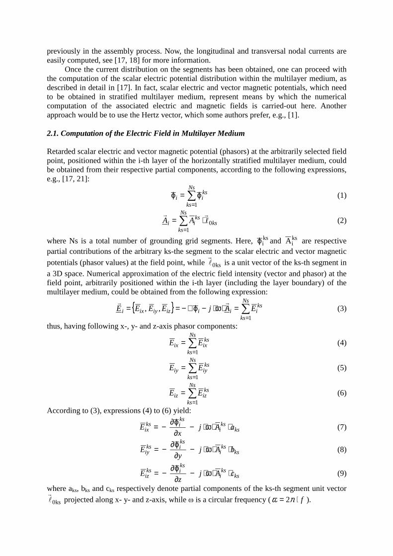
Hence, in accordance with the above stated facts, figure 2 displays a 3D surface plot of the x-component of the electric field (intensity magnitudes, i.e., effective values) at the field points forming the observational surface presented in the figure 1. At the same time, figure 3 graphically depicts a distribution of the effective values of the resultant / total electric field intensity along the same observational surface. Figures 2 and 3 should be compared with the appropriate figures published in [5, 6, 9], where a particularly good agreement could be observed -- both in terms of shape of the distribution and obtained numerical field values -- with results published in [5, 6]. In figure 3, we have obtained somewhat lover values of the electric field at the four field points of the observational surface directly above the grounding grid corners, compared to those of [5, 6]. However, when compared to the numerical results presented in [9], our agreement between figures 2 and 3 and those published in [5, 6] is better; the symmetry of the electric field distribution is particularly notable.

Figure 2 - Distribution of the x-component of the electric field magnitudes on the observational surface (60 Hz).

Figure 3 - Distribution of the resultant electric field magnitudes on the observational surface

(60 Hz). Figures 4 and 5 depict respectively x-component and resultant magnetic field intensity magnitudes (effective values) along the same observational surface at the ground level above the grounding grid at hand (see figure 1). Again, figures 4 and 5 should be compared with the appropriate figures published in [5, 6, 9]. Here, a particularly good agreement could be again observed -- both in terms of shape of the distribution and obtained numerical field values -- with results published in [5, 6]; the symmetry of the magnetic field distribution is particularly notable. The magnetic field in the field points directly above the current injection point is slightly higher in our case than found in [5, 6]. However, considering again the results published in [9], we have obtained better agreement with the results presented in [5, 6].

Figure 4 - Distribution of the x-component of the magnetic field magnitudes on the observational surface (60 Hz).

Figure 5 - Distribution of the resultant magnetic field magnitudes on the observational surface

(60 Hz). In order to asses the EM fields distribution in the higher frequency range, numerical

computation is repeated with the same input data, except for the frequency of the injected current which is now taken to be 500 kHz, again in accordance with treatment of [5, 6]. Consequently, figures 6 and 7 depict respectively resultant electric field intensity magnitudes and resultant magnetic field intensity magnitudes along the observational surface from figure 1 at this new frequency. It can be noted that these figures agree quite well with those published in [5, 6]. This in fact corroborates the applicability and validity of the presented numerical approach in computing the EM fields due to a system of conductors in horizontally stratified multilayer medium.

Figure 6 - Distribution of the resultant electric field magnitudes on the observational surface

(500 kHz).

Figure 7 - Distribution of the resultant magnetic field magnitudes on the observational surface

(500 kHz). Numerical computations were carried out on the following architecture: Intel Pentium D 3.0 GHz (3GB DDR2 RAM) on Ubuntu 10.04 OS (Linux kernel 2.6.32) with Intel Fortran Compiler for Linux 11.1 (-O2 optimization level). Average CPU time needed for the numerical solution of the treated problem is reported in the table 2. Table 2 – Average CPU time for the solution of the grounding grid treated in this example.

Numerical procedure CPU time (s) Data preparation, formation and solution of the global complex system of linear algebraic equations, determining current distribution on the grid segments

0.80

Computation of the resultant electric field intensity magnitudes in 6561 field points in multilayer medium

300

Computation of the resultant magnetic field intensity magnitudes in 6561 field points in multilayer medium

1.20

Total numerical solution 302 This CPU time could be further reduced (if needed) by interventions at the source code level, e.g., by implementing Intel MKL routines in place of the standard un-optimized LAPACK routines, as well as by adjusting the compiler switches for the targeted architecture. Further CPU time savings could be achieved by restructuring and fine-tuning the Fortran 95 source code of those routines for computing the electric field quantities, which has not been done at this stage. It ought to be mentioned here that in those cases of grounding grids where there is a large (i.e., predominant) number of non-horizontal conductors, CPU time could be significantly longer.

4. Conclusion This paper presented a numerical method for computing electromagnetic fields distribution in horizontally stratified multilayer medium, produced by the system of arbitrarily positioned harmonic current-carrying conductors. Presented numerical procedure forms an extension to the general electromagnetic model of the system of conductors in horizontally stratified multilayer medium, previously published by the authors, which has been able to compute scalar potential distributions in horizontally stratified multilayer medium. The model is based on the FET approach applied to the integral problem formulation in the frequency domain, with soil boundaries treated with a fixed image method and an approximation to the attenuation and phase shift effects. The validity of the method has been confirmed through the comparison of the numerically obtained results with those published by other authors (using different numerical approaches to the solution of this problem). It has been corroborated, as already indicated by other authors, that the distribution of the electric field intensity magnitude strongly depends on the frequency, while the magnetic field intensity magnitude is almost frequency independent. This electromagnetic model is general enough, in terms of the number of soil layers and position of conductors (which could penetrate the earth surface and extend into the air), to allow further scrutiny of the behavior of the EM fields above the transformer stations grounding grid, during, e.g., single-pole short circuit events (including complicated 3D geometry of the metallic structures represented by thin wires). Furthermore, analysis of the EM fields in the higher frequency range is also possible using the here presented numerical method. References [1] Dawalibi, F. P., Selby, A., “Electromagnetic Fields of Energized Conductors”, IEEE

Transactions on Power Delivery, Vol. 8, No.3, 1275-1284, 1993. [2] Dawalibi, F., “Electromagnetic Fields Generated by Overhead and Buried Short

Conductors, Part I – Single Conductor”, IEEE Transactions on Power Delivery, Vol. PWRD-1, No. 4, 105-111, 1986.

[3] Dawalibi, F., “Electromagnetic Fields Generated by Overhead and Buried Short Conductors, Part II – Ground Networks”, IEEE Transactions on Power Delivery, Vol. PWRD-1, No. 4, 112-119, 1986.

[4] Takasima, T., Nakae, T. S., Ishibashi, R., “High Frequency Characteristics of Impedances to Ground and Field Distributions of Ground Electrodes”, IEEE Transactions on Power Apparatus and Systems, Vol. PAS-100, No. 4, 1893-1900, 1981.

[5] Xiong, W., Dawalibi, F. P., “Transient Performance of Substation Grounding Systems Subjected to Lightning and Similar Surge Currents”, IEEE Transactions on Power Delivery, Vol. 9, No. 3, 1412-1420, 1994.

[6] Dawalibi, F. P., Xiong, W., Ma, J., “Transient Performance of Substation Structures and Associated Grounding Systems”, IEEE Transactions on Industry Applications, Vol. 31, No. 3, 520-527, 1995.

[7] Grcev, L., Dawalibi, F., “An Electromagnetic Model for Transients in Grounding Systems”, IEEE Transactions on Power Delivery, Vol. 5, No. 4, 1773-1781, 1990.

[8] Otero, A. F., Cidras, J., del Alamo, J. L., “Frequency-Dependent Grounding System Calculation by Means of a Conventional Nodal Analysis Technique”, IEEE Transactions on Power Delivery, Vol. 14, No. 3, 873-878, 1999.

[9] Nekhoul, B., et.al., “A Finite Element Method for Calculating the Electromagnetic Fields Generated by Substation Grounding Systems”, IEEE Transactions on Magnetics, Vol. 31, No. 3, 2150-2153, 1995.

[10] Selby, A., Dawalibi, F., “Determination of Current Distribution in Energized Conductors for the Computation of Electromagnetic Fields”, IEEE Transaction on Power Delivery, Vol. 9, No. 2, 1069-1078, 1994.

[11] Andolfato, R., Bernardi, L., Fellin, L., “Overhead and Buried Conductor System”, Proceedings of the 8th International Conference on Harmonics and Quality of Power, 14-18 October 1998, 1064-1070.

[12] Andolfato, R., Bernardi, L., Fellin, L., “Aerial and Grounding System Analysis by the Shifting Complex Images Method”, IEEE Transactions on Power Delivery, Vol. 15, No. 3, 1001-1009, 2000.

[13] Li, Z., Chen, W., Fan, J., Lu, J., “A Novel Mathematical Modeling of Grounding System Buried in Multilayer Earth”, IEEE Transactions on Power Delivery, Vol. 21, No. 3, 1267-1272, 2006.

[14] Zhang, B., et.al., “An Electromagnetic Approach to Analyze the Performance of the Substation’s Grounding Grid in High Frequency Domain”, COMPEL: The International Journal for Computation and Mathematics in Electrical and Electronic Engineering, Vol. 22, No. 3, 756-769, 2003.

[15] Baba, Y., Nagaoka, N., Ametani, A., “Modeling of Thin Wires in a Lossy Medium for FDTD Simulations”, IEEE Transactions on Electromagnetic Compatibility, Vol. 47, No. 1, 54-60, 2005.

[16] Vujević, S., Kurtović, M., “Numerical analysis of earthing grids buried in horizontally stratified multilayer earth”, International Journal for Numerical Methods in Engineering, Vol. 41, 1297–1319, 1998.

[17] Vujević, S., Sarajčev, P., Lovrić, D., “Time-harmonic analysis of grounding system in horizontally stratified multilayer medium”, Electric Power Systems Research, Vol. 83, 28-34, 2012.

[18] Sarajčev, P., Vujević, S., Lovrić, D., “Time-harmonic current distribution on conductor grid in horizontally stratified multilayer medium”, Progress in Electromagnetics Research B (PIER B), Vol. 31, 67-87, 2011.

[19] Sarajčev, P., Vujević, S., “Grounding Grid Analysis: Historical Background and Classification of Methods”, International Review of Electrical Engineering (IREE), Vol. 4, 670-683, 2009.

[20] Vujević, S., Sarajčev, P., “Potential distribution for a harmonic current point source in horizontally stratified multilayer medium”, COMPEL: The international journal for computation and mathematics in electrical and electronic engineering, Vol. 27, 624-637, 2008.

[21] Sarajčev, P., Electromagnetic model of the system of conductors in multilayer medium, PhD Dissertation, University of Split, Split, 2008 (in Croatian).

[22] Vujević, S., Sarajčev, P., Lucić, R., “Computing the mutual impedances between segments of earthing system conductors”, in Computational Methods and Experimental Measuremens XII, 641-650, WIT Press, Southampton, UK, 2005.