List of Papers

This thesis is based on the following papers, which are referred to in the textby their Roman numerals.

I Ranlöf, M., Perers R. and Lundin U., “On Permeance Modeling ofLarge Hydrogenerators With Application to Voltage Harmonics Predic-tion”, IEEE Trans. on Energy Conversion, vol. 25, pp. 1179-1186, Dec.2010.

II Ranlöf, M. and Lundin U., “The Rotating Field Method Applied toDamper Loss Calculation in Large Hydrogenerators”, Proceedings ofthe XIX Int. Conf. on Electrical Machines (ICEM 2010), Rome, Italy,6-8 Sept. 2010.

III Wallin M., Ranlöf, M. and Lundin U., “Reduction of unbalanced mag-netic pull in synchronous machines due to parallel circuits”, submittedto IEEE Trans. on Magnetics, March 2011.

IV Ranlöf, M., Wolfbrandt, A., Lidenholm, J. and Lundin U., “Core LossPrediction in Large Hydropower Generators: Influence of RotationalFields”, IEEE Trans. on Magnetics, vol. 45, pp. 3200-3206, Aug. 2009.

V Ranlöf, M. and Lundin U., “Form Factors and Harmonic Imprint ofSalient Pole Shoes in Large Synchronous Machines”, accepted for pub-lication in Electric Power Components and Systems, Dec. 2010.

VI Ranlöf, M. and Lundin U., “Finite Element Analysis of a PermanentMagnet Machine with Two Contra-rotating Rotors”, Electric PowerComponents and Systems, vol. 37, pp. 1334-1347, Dec. 2009.

VII Ranlöf, M. and Lundin U., “Use of a Finite Element Model for theDetermination of Damping and Synchronizing Torques of Hydroelec-tric Generators”, submitted to The Int. Journal of Electrical Power andEnergy Systems, May 2010.

VIII Ranlöf, M., Wallin M. , Bladh J. and Lundin U., “Experimental Studyof the Effect of Damper Windings on Synchronous Generator Hunting”,submitted to Electric Power Components and Systems, February 2011.

IX Lidenholm J., Ranlöf, M. and Lundin U., “Comparison of field andcircuit generator models in single machine infinite bus system simula-tions”, Proceedings of the XIX Int. Conf. on Electrical Machines (ICEM2010), Rome, Italy, 6-8 Sept. 2010.

v

X Wallin M., Ranlöf, M. and Lundin U., “Design and construction of asynchronous generator test setup”, Proceedings of the XIX Int. Conf. onElectrical Machines (ICEM 2010), Rome, Italy, 6-8 Sept. 2010.

Reprints were made with permission from the publishers.

vi

Contents

1 Introduction . . . . . . . . . . . . . . . . . . . . . . . . . . . . . . . . . . . . . . . . . . 11.1 Background . . . . . . . . . . . . . . . . . . . . . . . . . . . . . . . . . . . . . . . 11.2 Applications of Permeance Models of Salient-pole Generators . 21.3 Core Loss Prediction in Large Hydropower Generators . . . . . . 31.4 Form Factors of Salient Pole Shoes . . . . . . . . . . . . . . . . . . . . . 31.5 Analysis of a PM Generator with Two Contra-rotating Rotors . 41.6 Electromechanical Transients - Simulation and Experiments . . 41.7 Outline of the Thesis . . . . . . . . . . . . . . . . . . . . . . . . . . . . . . . . 5

2 Theory . . . . . . . . . . . . . . . . . . . . . . . . . . . . . . . . . . . . . . . . . . . . . . 72.1 Salient-pole Synchronous Generators . . . . . . . . . . . . . . . . . . . . 7

2.1.1 Main Construction Elements . . . . . . . . . . . . . . . . . . . . . . 72.1.2 Grid-connected Operation . . . . . . . . . . . . . . . . . . . . . . . . 9

2.2 Equivalent Circuit Generator Model . . . . . . . . . . . . . . . . . . . . . 102.2.1 P.U. Electrical Equations . . . . . . . . . . . . . . . . . . . . . . . . . 11

2.3 Finite Element Generator Model . . . . . . . . . . . . . . . . . . . . . . . 132.3.1 Calculation Geometry and Material Property Assignment . 132.3.2 Field Equation Formulation . . . . . . . . . . . . . . . . . . . . . . . 142.3.3 Finite Element Discretization . . . . . . . . . . . . . . . . . . . . . . 162.3.4 Boundary Conditions . . . . . . . . . . . . . . . . . . . . . . . . . . . . 172.3.5 Calculation of Air-gap Torque and Induced EMF . . . . . . . 18

2.4 Coupled Field-circuit Models . . . . . . . . . . . . . . . . . . . . . . . . . . 192.4.1 Coupling Equations for Circuit-connected Conductors . . . 192.4.2 Rated Voltage No-load Operation Model . . . . . . . . . . . . . 202.4.3 Balanced and Unbalanced Load Models . . . . . . . . . . . . . . 232.4.4 Grid-connected FE Model with Mechanical Equation . . . . 25

3 Applications of Permeance Models of Salient-pole Generators . . . . 273.1 Previous Work . . . . . . . . . . . . . . . . . . . . . . . . . . . . . . . . . . . . . 273.2 Permeance Model Implementation . . . . . . . . . . . . . . . . . . . . . . 28

3.2.1 Coordinate System . . . . . . . . . . . . . . . . . . . . . . . . . . . . . . 283.2.2 Field and Armature MMF Functions . . . . . . . . . . . . . . . . 293.2.3 Pole Shape Permeance Function . . . . . . . . . . . . . . . . . . . . 313.2.4 Saturation and Stator Slot Permeance Functions . . . . . . . . 31

3.3 Damper Winding MMF and Circuit Equations . . . . . . . . . . . . . 333.3.1 Flux Density Harmonics . . . . . . . . . . . . . . . . . . . . . . . . . 343.3.2 Unitary Damper Loop MMF Functions . . . . . . . . . . . . . . 363.3.3 Calculation of Damper Loop Currents . . . . . . . . . . . . . . . 37

vii

3.3.4 Resultant Damper MMF . . . . . . . . . . . . . . . . . . . . . . . . . 403.4 Selected Results . . . . . . . . . . . . . . . . . . . . . . . . . . . . . . . . . . . 41

3.4.1 THD of the Open-circuit Armature Voltage Waveform . . . 413.4.2 Damper Bar Currents at Rated Load Operation . . . . . . . . . 423.4.3 Reduction of the UMP by Parallel Armature Circuits . . . . 43

4 Core Loss Prediction in Large Hydroelectric Generators . . . . . . . . . 454.1 Previous Work . . . . . . . . . . . . . . . . . . . . . . . . . . . . . . . . . . . . . 454.2 Iron Loss Estimation . . . . . . . . . . . . . . . . . . . . . . . . . . . . . . . . 45

4.2.1 Loss Separation . . . . . . . . . . . . . . . . . . . . . . . . . . . . . . . . 454.2.2 Rotational Losses . . . . . . . . . . . . . . . . . . . . . . . . . . . . . . . 46

4.3 Study Summary . . . . . . . . . . . . . . . . . . . . . . . . . . . . . . . . . . . . 484.4 Selected Results . . . . . . . . . . . . . . . . . . . . . . . . . . . . . . . . . . . 50

5 Form Factors of Salient Pole Shoes . . . . . . . . . . . . . . . . . . . . . . . . 535.1 Background . . . . . . . . . . . . . . . . . . . . . . . . . . . . . . . . . . . . . . . 535.2 Pole Shoe Form Factors . . . . . . . . . . . . . . . . . . . . . . . . . . . . . . 545.3 Study Summary . . . . . . . . . . . . . . . . . . . . . . . . . . . . . . . . . . . . 55

5.3.1 Pole Face Contours . . . . . . . . . . . . . . . . . . . . . . . . . . . . . 565.3.2 Pole Shoe Variables . . . . . . . . . . . . . . . . . . . . . . . . . . . . . 57

5.4 Selected Results . . . . . . . . . . . . . . . . . . . . . . . . . . . . . . . . . . . 585.4.1 Effect of Pole Face Contour . . . . . . . . . . . . . . . . . . . . . . . 585.4.2 Linear Models with Saturation Considered . . . . . . . . . . . . 595.4.3 Perspectives on Pole Shoe Shape Selection . . . . . . . . . . . . 60

6 Analysis of a PM Generator with Two Contra-rotating Rotors . . . . . 616.1 Previous Work . . . . . . . . . . . . . . . . . . . . . . . . . . . . . . . . . . . . . 616.2 Generator Topology . . . . . . . . . . . . . . . . . . . . . . . . . . . . . . . . . 61

6.2.1 Dual Contra-rotating Rotor Topology . . . . . . . . . . . . . . . . 616.2.2 Reference Machine Topologies . . . . . . . . . . . . . . . . . . . . 62

6.3 Selected Results . . . . . . . . . . . . . . . . . . . . . . . . . . . . . . . . . . . 636.3.1 Characterization of the Inter-rotor Cross Coupling . . . . . . 636.3.2 Synchronized Contra-rotating Load Operation . . . . . . . . . 66

7 Electromechanical Transients - Simulation and Experiments . . . . . . 697.1 Previous Work . . . . . . . . . . . . . . . . . . . . . . . . . . . . . . . . . . . . . 697.2 Rotor Angle Oscillations . . . . . . . . . . . . . . . . . . . . . . . . . . . . . 69

7.2.1 The Swing Equation . . . . . . . . . . . . . . . . . . . . . . . . . . . . 707.2.2 Damping and Synchronizing Torques . . . . . . . . . . . . . . . . 71

7.3 Study Summary . . . . . . . . . . . . . . . . . . . . . . . . . . . . . . . . . . . . 737.3.1 Torque Coefficient Determination from a Field Model . . . 737.3.2 Experimental Study . . . . . . . . . . . . . . . . . . . . . . . . . . . . . 73

7.4 Selected Results . . . . . . . . . . . . . . . . . . . . . . . . . . . . . . . . . . . 747.4.1 Comparison of Field and Circuit Model Responses . . . . . . 747.4.2 Experimental Study . . . . . . . . . . . . . . . . . . . . . . . . . . . . . 76

8 Conclusions . . . . . . . . . . . . . . . . . . . . . . . . . . . . . . . . . . . . . . . . . . 819 Suggested Future Work . . . . . . . . . . . . . . . . . . . . . . . . . . . . . . . . . 8310 Summary of Papers . . . . . . . . . . . . . . . . . . . . . . . . . . . . . . . . . . . . 87

viii

11 Summary in Swedish . . . . . . . . . . . . . . . . . . . . . . . . . . . . . . . . . . . 93Acknowledgment . . . . . . . . . . . . . . . . . . . . . . . . . . . . . . . . . . . . . . . . . 95References . . . . . . . . . . . . . . . . . . . . . . . . . . . . . . . . . . . . . . . . . . . . . . 97

ix

List of Symbols and Abbreviations

Fields

Symbol Unit Definition

A Tm Magnetic vector potential

B T Magnetic flux density / induction

H A/m Magnetic field

J A/m2 Current density

Scalars

Symbol Unit DefinitionAz Tm Z-component of magnetic vector potentialbp m Pole body widthBgm T Peak value of air-gap flux density waveBmax T Peak flux densityΔBr T Radial flux density distortionei V Induced EMF in armature phase i (i =

a,b,c) (field model)ed p.u. Direct-axis armature voltage (equivalent

circuit model)e f d p.u. Field voltage (equivalent circuit model)eq p.u. Quadrature-axis armature voltage (equi-

valent circuit model)E V or p.u. Internal EMFf Hz Electrical frequencyfa - Pole taperf0 Hz Hunting frequencyhpp m Pole shoe heightH s Inertia constant

xi

Scalars (continued)

Symbol Unit Definition

i j A Current in armature phase j ( j = a,b,c)

id p.u. Direct-axis armature current

i f d p.u. Field winding current (equivalent circuitmodel)

iq p.u. Quadrature-axis armature current

i1d p.u. Direct-axis damper current

i1q p.u. Quadrature-axis damper current

I f A Field current

J kgm2 Moment of inertia

kc Sm4/kg Classical loss coefficient

kd - Direct-axis armature pole shoe form factor

kE Am3V−0.5kg−1 Excess loss coefficient

k f - Field winding pole shoe form factor

kH Am4(V s kg )−1 Hysteresis loss coefficient

kq - Quadrature-axis armature pole shoe formfactor

Kd p.u. torque /(rad/s)

Damping torque coefficient

Ks p.u. torque / rad Synchronizing torque coefficient

le m Effective machine length

Lad p.u. Direct-axis mutual inductance

Laq p.u. Quadrature-axis mutual inductance

Le H Armature end-winding leakage inductance

Lfd p.u. Field leakage inductance

Ll p.u. Armature leakage inductance

L1d p.u. Direct-axis damper winding leakage in-ductance

L1q p.u. Quadrature-axis damper winding leakageinductance

Ma A·turns Armature winding MMF

MD A·turns Damper winding MMF

Mf A·turns Field winding MMF

xii

Symbol Unit Definition

n rpm Rotational speed

Nd - Number of damper bars per pole

Nf - Number of field winding turns per pole

Np - Pole pair number

q1 - Number of stator slots per pole and phase

ptot W/kg Total specific iron loss

Padd−dyn % Fractional loss increase due to rotationaland harmonic fields

Padd−rot % Fractional loss increase due to rotationalfields

Ra p.u. Armature phase resistance

Rc Ω Inter-pole end-ring resistance

Re Ω Armature end-winding resistance

Rfd p.u. Field winding resistance

R1d p.u. Direct-axis damper winding resistance

R1q p.u. Quadrature-axis damper winding resis-tance

S m2 Conductor area

Te Nm or p.u. Electrical torque

ΔTe p.u. Change in electrical torque

Un V or p.u. Rated terminal voltage (RMS, line-to-line)

V V Electric potential / applied voltage (fieldmodel)

Xd Ω or p.u. Direct-axis synchronous reactance

Xq Ω or p.u. Quadrature-axis synchronous reactance

Zb Ω Damper bar impedance

Γ - Degree of rotation

δ Elect. rad. Rotor (load) angle (Chapters 2 and 7)

δ m Air-gap length (Chapter 5)

Δδ Elect. rad. Rotor angle deviation

θ Elect. rad. Electrical angular coordinate

θm Mech. rad. Mechanical angular coordinate

Λ Vs/(Am2) Air-gap permeance function

Λecc - Eccentricity permeance function

xiii

Scalars (continued)

Symbol Unit Definition

ΛP m−1 Pole-shape permeance function

Λsat - Saturation permeance function

ΛSslot - Stator slot permeance function

μr - Relative magnetic permeability

μ0 Vs/(Am) Permeability of free space

ν m/H Magnetic reluctivity

σ S/m Electric conductivity

τD s Damping time constant

τds - Damper slot pitch

τp m Pole pitch

τpc m / - Concentric pole shoe width

τpp m / - Pole shoe width

τs m Stator slot pitch

φ Elect. rad. Power factor angle

Ψ Wb turns / p.u. Flux linkage

Ψad p.u. Direct-axis mutual (air-gap) flux linkage

Ψaq p.u. Quadrature-axis mutual (air-gap) flux link-age

Ψd p.u. Direct-axis armature winding flux linkage

Ψ f d p.u. Field winding flux linkage

Ψq p.u. Quadrature-axis armature winding fluxlinkage

Ψ1d p.u. Direct-axis damper winding flux linkage

Ψ1q p.u. Quadrature-axis damper winding flux link-age

ω Elect. rad/s Electrical angular frequency

ωm Mech. rad/s Mechanical angular frequency

ωms Mech. rad/s Synchronous angular frequency

ωs Elect. rad/s Synchronous angular frequency

ω0 Mech. rad/s Hunting angular frequency

Δω p.u. Angular frequency (speed) deviation

xiv

Abbreviations

AC Alternating Current

DC Direct Current

EC Equivalent Circuit

EMF Electromotive Force

FE Finite Element

FEA Finite Element Analysis

FEM Finite Element Method

MMF Magnetomotive Force

PM Permanent Magnet

p.u. Per Unit

SiFe Silicon-Iron alloy

SMIB Single Machine Infinite Bus

THD Total Harmonic Distortion

UMP Unbalanced Magnetic Pull

xv

1. Introduction

1.1 BackgroundLarge-scale exploitation of hydropower resources in Sweden started in the firstdecades of the 20th century. The clean and controllable supply of power fromhydropower plants was vital for the electrification of the society and the de-velopment of the Swedish industry throughout the century. Today, hydropowerstill remains an essential ingredient in the national energy mix, and accountsfor 46%1 of the country’s annual electricity production of 145 TWh [1]. Reli-able and efficient operation of the hydropower plants is crucial, and this callsfor safe and professionally designed plant components.

The generator is one of the key components of a hydropower plant, sinceit constitutes the site for the conversion between mechanical and electricalenergy. The work presented in this doctoral thesis is a part of a researchprogram devoted to hydropower generator technology at Uppsala University,initiated by The Swedish Hydropower Centre (Svenskt Vattenkraftcentrum,SVC). SVC is a national collaboration platform for power suppliers, manu-facturers of hydropower equipment, consulting agencies, The Swedish EnergyAgency, The Swedish National Grid Agency and five technical universities.SVC’s vision is to promote the provision of qualified human resources to allbranches of the national hydropower industry in order to secure an efficientand safe production of hydro electricity in the future, and to secure a main-tained dam safety2.

The scientific aim of the doctoral project was to address subjects associ-ated with electromagnetic analysis of synchronous machines with a particularemphasis on grid-connected operation of hydroelectric generators. Because ofthe general formulation of scope of the project, the work comprises a set ofdiversified studies.

The field of synchronous machine analysis encompasses both electric, mag-netic, thermal and mechanical aspects. As the title of the thesis indicates, thework presented here is largely limited to electric and magnetic phenomena.Electromagnetic analysis is here defined as the study of electric currents, mag-netic fields, electric voltages and power flows in an apparatus during steady-state and transient operating conditions. The scope of the work is somewhat

1Calculated average between the years 2000-2008.2www.svc.nu. Accessed on January 12 2011.

1

extended with a simple model of electromechanical interaction in studies onsynchronous machine hunting (see Chap. 7).

The studies that are presented in this comprehensive summary can be di-vided into five main subjects. The ten papers, which constitute the founda-tion of the thesis, are in turn subordinate to either of these five subjects. Thefirst main subject will be referred to as applications of permeance models ofsalient-pole generators. A series of papers (I, II, and III) fall under this subject.The second subject is core loss prediction. A single publication (Paper IV) be-longs to this category. The third subject is entitled form factors of salient poleshoes, and is represented by Paper V. The fourth main subject concerns anon-conventional permanent magnet (PM) generator topology and is labeledanalysis of a PM generator with two contra-rotating rotors. Paper VI em-bodies this subject. The final subject is electromechanical transients. Variousaspects of this topic are discussed in Papers VII, VIII, and IX. The last paper,Paper X, deals with design considerations for an experimental generator setupand is the only publication not to fall under any of the main subjects.

In spite of the diversity of the addressed problems, some studies that be-long to different main subjects share common denominators. For instance, thedamper winding end-ring connection is discussed both in terms of its impacton the armature voltage waveform distortion (Papers I and X) as well as itsmitigating effects on rotor angle oscillations (Papers VII and VIII). Moreover,all studies but one (Paper VI), are concerned with the conventional vertical-axis machine topologies that are typically encountered in large hydropowerplants.

In the following sections, the five main subjects are briefly introduced andthe objectives of the individual studies are stated. The chapter is concludedwith a presentation of the outline of the thesis.

1.2 Applications of Permeance Models of Salient-poleGeneratorsThe rotating field method determines the air-gap flux density in an electricalmachine as the product of a magnetomotive force (MMF) and a permeancefunction. A calculation scheme that uses this approach to derive the air-gapflux density is referred to as a permeance model. In combination with circuitequations that represent the damper winding, it is possible to determine ap-proximately the full air-gap flux density waveform, including the harmoniccontribution of the damper reaction [2]. Different applications of the perme-ance modeling technique for synchronous generators with salient, laminatedpoles are explored in Papers I, II, and III.

The aim of the study presented in Paper I was to develop a permeance modelsuitable for the calculation of open-circuit armature voltage harmonics. In thestudy summarized in Paper II, the objective was to explore the applicability

2

of the model in studies of steady balanced and unbalanced load operation.Finally, in Paper III, the objective was to assess the usefulness of the perme-ance model in predicting the effects of parallel armature circuits on a steadyunbalanced magnetic pull (UMP).

1.3 Core Loss Prediction in Large HydropowerGeneratorsIn the conversion between mechanical and electrical energy that takes placein a generator, a certain amount of power is continuously converted to heatthrough various dissipation mechanisms. This is the loss of the conversionscheme. The term core loss refers to the power loss that is developed in theiron core of the stator. Core losses are fundamentally attributable to the eddycurrents that arise in the stator laminations upon exposure of a time-varyingmagnetic flux. Besides the macroscopic eddy current loss, the internal mag-netic domain structure of the soft ferromagnetic steel used in stator lamina-tions gives rise to additional loss components - hysteresis and excess losses -that also add to the core loss.

As high machine efficiency is a prioritized objective, iron loss studies con-tinuously generates many scientific papers. Recently addressed problems inthis field include improved material modeling [3, 4], the influence of bidirec-tional magnetic fields (“rotational losses”) [5–8], time-saving analytical losscalculations [9–11], and loss predictions from 3-D magnetic field computa-tions [12].

The goal of the project that resulted in Paper IV was to evaluate the corelosses in twelve large hydroelectric generator topologies, using iron loss pre-diction models of varying complexity. An equally important goal was to as-sess the importance of the additional loss introduced by bidirectional magneticfields in these machines.

1.4 Form Factors of Salient Pole ShoesHydroelectric generators are typically equipped with salient rotor poles, andthe shape of the pole shoe directly affects the appearance of the air-gap fluxdensity waveform. In order to determine the inductances of fundamental waveequivalent circuit representations of synchronous machines, the correlationbetween the fundamental wave amplitude and the maximum wave amplitudeis required. To this end, pole shoe form factors are introduced in the math-ematical expressions of the different machine inductances. Form factors aredefined for three reference cases of magnetic excitation and can be said tocharacterize the pole shoe shape.

3

In the technical literature, many studies on salient pole shoe design andform factors date from the first part of the 20th century [13, 14]. These earlystudies are founded on analysis techniques that neglect iron saturation andhigher order harmonics of the impressed MMF waveforms. The validity ofthe results for all the practical pole face contour designs that are in use isalso unclear. Even so, the results of these studies are usually cited in moderntextbooks of synchronous machine design [15].

The primary objective of the work presented in Paper V was to study theeffect of iron saturation on pole shoe form factors. The study was howeverextended to embrace a more general comparison of different pole face con-tour designs from a form factor perspective. Moreover, the harmonic imprintof different salient pole shoes on the air-gap flux density waveform was con-sidered.

1.5 Analysis of a PM Generator with TwoContra-rotating RotorsHydraulic turbine concepts with two contra-rotating impellers have been pre-sented both for use in small-scale hydropower plants [16] and in tidal energyconversion schemes [17]. The benefits of employing a turbine with two contra-rotating stages include a near-zero reaction torque on the support structure,near-zero swirl in the wake and high relative rotational speeds. For a com-plete energy conversion system employing such a turbine, a generator withtwo contra-rotating rotors and one single stator winding is an interesting, butunexplored machine concept. Caricchi et al. performed one of the rare studieson this particular type of machine topology [18]. Their communication reportsof an axial flux motor with two contra-rotating rotors designed to operate in aship propulsion drive.

Motivated by the possible applicability in small-scale hydro schemes aswell as the relative sparsity of available information on electrical machineswith contra-rotating rotors, a research project aimed at exploring further theoperating characteristics of this machine topology was initiated. A selectionof findings are reported in Paper VI.

1.6 Electromechanical Transients - Simulation andExperimentsDuring perfect steady-state operation of a grid-connected synchronous gener-ator, the speed of the rotor is identical to the synchronous speed dictated bythe mains frequency. The term electromechanical transient will be used here

4

to denote temporary rotor speed excursions around the synchronous speed,and the associated fluctuations in electrical torque.

From a physical perspective, the grid-connected generator is in close anal-ogy with a mechanical arrangement consisting of a discrete mass attachedto a wall through a spring and a damper. Electric spring and damper actionduring rotor swings results from the interaction between the rotor and sta-tor circuits, and is described in terms of synchronizing and damping torques.Because of their importance for stable operation of inter-connected power sys-tems, damping and synchronizing torques of synchronous machines have beenextensively studied in the past [19–23].

While previous studies have addressed damping and synchronizing torquecalculation with analytical formulae, the objective of the study presented herewas to determine these machine properties from numerical field simulations.To this end, a coupled field-circuit model of the classical single machineinfinite bus (SMIB) system was developed. Papers VII and IX describe theoutcome of the numerical experiments performed with this model, whilePaper VIII is concerned with the experimental determination of the naturaldamping properties of a laboratory generator. Particular attention is devotedto the effect of different damper winding configurations.

1.7 Outline of the ThesisDue to the diversity of the research studies, the author has preferred to devoteone chapter to each main subject. Each subject chapter contains a descriptionof the method of analysis and a few, selected results. This unconventionaloutline was deliberately chosen to facilitate for readers who take interest inone particular subject.

The first part of Chapter 2 contains a short introduction on the function andthe main construction elements of salient-pole synchronous generators. Thesecond part of Chapter 2 discusses equivalent circuit (EC) and finite element(FE) models of synchronous electric machines. The chapter is then concludedwith a presentation of the coupled field-circuit models that were used in thedifferent studies. Next, Chapters 3-7 are devoted to the respective main sub-jects. Permeance model applications are treated in Chapter 3, core losses inChapter 4, and pole shoe form factors in Chapter 5. Chapter 6 and Chapter 7are devoted to analysis of a PM generator with two contra-rotating rotors andelectromechanical transients respectively. Conclusions are presented in Chap-ter 8 and suggestions for future studies are given Chapter 9.

5

2. Theory

This chapter is intended to serve two purposes. The first purpose is to providenon-expert readers with some useful notions which will assist digestion of thecontents of Chapters 3-7. The second purpose is to provide professional read-ers with comprehensive mathematical descriptions of the EC and FE modelsof synchronous generators that have been used in the different studies. In aspirit of compromise between these aims, some general information on ECand FE models of synchronous generators, which the author deemed manda-tory, is also provided.

Section 2.1 describes the main construction elements of hydroelectric gen-erators. In Section 2.2, EC models of synchronous generators are briefly dis-cussed. Furthermore, the EC model structure used in Papers VII, VIII andIX is presented. Next, Section 2.3 provides an introduction to FE generatormodels. Section 2.4 finally presents the mathematical structure of the coupledfield-circuit models that have been used in the different studies.

2.1 Salient-pole Synchronous Generators2.1.1 Main Construction ElementsThe purpose of a generator is to convert mechanical energy, supplied from aprime mover via a rotating shaft, to electric energy, which is typically fed intothe power grid. This electromechanical energy conversion is realized with themagnetic field inside the generator acting as an intermediate coupling.

Most generators in large hydropower plants are synchronous generatorswith salient rotor poles. The word “large” here denotes a generator in the MWrange. In the past, horizontal-axis units were common, but today, the majorityof the hydro generating units are built as vertical-axis machines.

The two main parts of a conventional hydroelectric generator are the statorand the rotor. The stator consists of a circular magnetic iron core, constructedfrom thin silicon steel sheets and supported by a steel frame. The inner sta-tor periphery holds uniformly stamped slots, where a three-phase winding isinserted. This is the armature or stator winding. The winding is typically com-posed of form-wound copper coils insulated with a high voltage mica-basedinsulation system.

The rotor, or pole wheel, is attached to the rotating shaft. It consists of aframe, an iron ring made from stacked steel sheets, and rotor poles. The rotor

7

Figure 2.1: (a) Axial cross-section of a salient-pole synchronous machine with fourpoles. 1. Pole body. 2. Pole shoe. 3. Field coils. 4. Stator winding coils. 5. Damperwinding.

is separated from the stationary stator by an air-gap. The rotor poles, alsoconstructed from laminated steel sheets, hold the field winding, that providesthe fundamental magnetic field excitation.

Fig. 2.1 shows the axial cross-section of a four-pole synchronous machinewith salient poles. The part of the pole which is closest to the air-gap is re-ferred to as the pole shoe. The pole shoes of large synchronous machines typ-ically hold copper or brass bars. This is the amortisseur or damper winding.The bars in adjacent poles can be connected via a short-circuit ring in bothmachine ends. This configuration is referred to as a complete or a continuousdamper winding.1 A damper winding that lacks the inter-pole connection like-wise has many designations in the technical literature. Any of the terms open,incomplete, non-continuous, or grill damper winding can be used to denotethis damper winding configuration.

To deal with the asymmetric air-gap produced by the pole saliency, it isconvenient to introduce two sets of rotor-fixed reference axes - the direct (d)and quadrature (q) axes (see Fig. 2.1). A d-axis is aligned with the center axis

1Some prefer to refer to this configuration simply as a squirrel cage winding.

8

of a north pole. The q-axes go through inter-polar gaps adjacent to and leadingthe d-axes.

2.1.2 Grid-connected OperationMost of the global electric energy generation is performed throughsynchronous generators connected to three-phase alternating current (AC)power grids. The rotational speed, n, of a grid-connected synchronousgenerator is given by

n = 60 · fNp

[rpm], (2.1)

where f is the grid frequency and Np denotes the number of pole pairs in thegenerator. n is referred to as the synchronous or rated speed of the unit.

During normal load operation, balanced three-phase currents in the arma-ture winding phases produce a magnetic field that rotates at synchronousspeed. This field is called the armature reaction. The fundamental waves ofthe armature reaction and the rotor excitation field have the same number ofpoles and are at standstill with respect to each other. Through the interactionbetween these fields, a non-zero synchronous torque is produced which tendto align the fields with each other. During balanced load operation, the anglebetween the rotor and the armature fields is more or less constant, and the syn-chronous torque production is manifested as a continuous transfer of power tothe AC grid.

The steady active and reactive power productions, Pg and Qg, from a syn-chronous generator are approximately given by

Pg =3EUXd

sinδ +32U2

(1Xq− 1

Xd

)sin2δ

Qg =3EUXd

cosδ −3U2(

cos2δXd

+sin2δXq

).

(2.2)

In the above expressions, the resistive losses in the stator winding are ne-glected. E is the so called internal EMF (here, an RMS phase quantity inVolts), U is the terminal voltage (RMS phase quantity in Volts), and Xd (Ω)and Xq (Ω) denote the synchronous reactances in the direct- and quadratureaxes respectively. δ is the load angle (or rotor angle), and corresponds to thephase angle between the voltages E and U . The function Pg(δ ) is called theactive power - load angle characteristics of the synchronous generator and isschematically illustrated in Fig. 2.2.

During normal operation, the synchronous generator operates at a load an-gle that is considerably smaller than the critical load angle, δC. The angle δC

corresponds to the maximal active power delivery at a given level of excita-

9

Figure 2.2: Active power versus load angle (synchronous generator).

tion. The generator is considered to be stable with respect to slow shaft torqueor load variations as long as the load angle does not exceed δC

2 [24].

2.2 Equivalent Circuit Generator ModelIn studies of the electromagnetic interaction between synchronous generatorsand other electrical equipment, the generators are frequently represented bya set of electrical circuit equations. A long tradition of elaborate refinementand adaptation of such circuit representations to fit almost any problem ofinterest, makes this the most established and accessible form of generatoranalysis. A number of factors determine the nature of a generator EC model.Some of the most important factors are briefly discussed in the following.

Nominal or P.U. Representation of Model VariablesModel quantities can be represented with physical units (V, A, W e.t.c) or,

alternatively, units are eliminated from the calculations by expressing allquantities in terms of fractions of specified base values. The latter approachis called per unit (p.u.) representation. The p.u. representation is convenientin power systems with many different voltage levels, and also facilitates thecomparison of electrical arrangements with dissimilar power ratings.

Winding RepresentationThe armature can be modeled by its three physical stationary armature

phases A, B, and C or, alternatively, by means of fictitious rotor-fixed wind-ings. A stator-fixed representation is usually referred to as a phase domainmodel, while the rotor-fixed representation is called a dq0 or two-axis model.

2This is the static stability of the generator, and is defined as the ability of the generator toremain in synchronism with the power grid when subjected to slow shaft power or load varia-tions.

10

Two-reaction theory, which forms the basis of two-axis representations of syn-chronous machines, was originally worked out by Blondel [25].

The dq0-representation brings about numerous modeling advantages, suchas time-independent circuit inductances and decoupling of the d- and q-axiscircuits if iron saturation is neglected. The approach involves the applicationof the Park transformation to all stator quantities [26].

In power system analysis software, the internal electrical representationsof synchronous machines are almost exclusively in dq0-coordinates. Applica-tions of physical armature phase representation in EC models however do ex-ist. A prominent example is the analysis of internal short-circuit faults [27,28].

The representation of the rotor windings primarily concerns the structureof the equivalent damper winding circuits [29, 30]. The level of modelingdetail should be adjusted to the problem at hand and the required accuracy ofthe results.

Consideration of Non-Linear and Harmonic EffectsMost dq0-models are fundamental wave models, that is, they only consider

the dominating space fundamentals of the magnetic flux density waves insidethe generator. Linear EC models either neglect iron saturation or representthe effect by parameter values appropriate at the studied point of operation(“saturated parameters”). Iron saturation can alternatively be accounted forwith refined iterative methods [31]. It is also possible to account for someharmonic effects on generator performance [32].

Choice of Independent State VariablesThe selection of independent state variables depends on the circuit repre-

sentation [33]. For fundamental parameter circuit representations, windingflux linkages and currents are preferably used. In some applications, a mixedor “hybrid” choice of independent variables may be the best choice [34].

2.2.1 P.U. Electrical EquationsEC generator models were used in the studies presented in Papers VII, VIIIand IX. The employed circuit model was a dq0-model with one damper circuitin each axis, which is customary for rotor angle stability studies of hydroelec-tric generating units. The model was represented in the conventional Lad-basereciprocal p.u. system. In Paper IX, the circuit parameters were derived fromFE simulations of standard parameter determination tests [35]. In Papers VIIand VIII, the parameters were calculated from generator design data. The em-ployed analytic parameter calculation formulae were taken from [15] and [36].

The p.u. electrical equations of the EC model are listed below. All variables,including time, are given in p.u. Zero-sequence equations are omitted, sinceonly balanced generator operation was considered in the studies where a cir-cuit model was used. The system of differential-algebraic equations used to

11

Figure 2.3: Circuit representation of voltage and flux linkage equations. Top: d-axiscircuit. Bottom: q-axis circuit.

simulate the SMIB systems of Papers VII and IX, can be derived from the ex-pressions below, except for the two equations that describe the grid coupling.These equations are summarized in Paper IX.

The listed equations can be represented with the equivalent d- and q-axiscircuits shown in Fig. 2.3. The notation follows that used in IEEE Std. 1110-2002 [29], but for completeness all symbols are also described in the List ofSymbols.

Stator voltage equations

ed =dΨd

dt−Ψqω−Raid (2.3)

eq =dΨq

dt+Ψdω−Raiq (2.4)

Rotor voltage equations

e f d =dΨ f d

dt+Rfdi f d (2.5)

0 =dΨ1d

dt+R1di1d (2.6)

0 =dΨ1q

dt+R1qi1q (2.7)

Stator flux linkage equations

Ψd = −(Lad +Ll)id +Ladi f d +Ladi1d (2.8)

Ψq = −(Laq +Ll)iq +Laqi1q (2.9)

12

Rotor flux linkage equations

Ψ f d = −Ladid +(Lad +Lfd)i f d +Ladi1d (2.10)

Ψ1d = −Ladid +Ladi f d +(Lad +L1d)i1d (2.11)

Ψ1q = −Laqiq +(Laq +L1q)i1q (2.12)

Air-gap torqueTe = Ψadiq−Ψaqid (2.13)

2.3 Finite Element Generator ModelIn equivalent circuit models, the inherently distributed nature of the electro-magnetic interaction inside the generator is “lumped” into a fairly limited setof equations. We here define a field generator model as a model that deter-mines the electrical performance directly from the magnetic field distributionin the active parts (stator, air-gap, rotor) of the generator.

The magnetic field distribution is determined from Ampères law, whichneeds to be appropriately formulated for the application at hand. The prob-lem of solving the field equations by means of digital computing can then betackled with a variety of numerical methods. For electromagnetic analysis ofelectrical machines, the Finite Element Method (FEM) has emerged as themost widely applied numerical method. Its popularity is linked to its ability tohandle the complicated calculation geometries presented by rotating machin-ery [37].

FEM was originally used to study problems in structural mechanics. Itsemployment for the solution of the electromagnetic vector field problems pre-sented by electric machinery became widely diffused in the 1980’s [38, 39].Today, FE analysis is more or less a standard tool in electrical machine de-sign, and the method can be used to study problems of both electromagnetic,thermal, mechanical and coupled (“multiphysics”) nature. There exists a num-ber of commercial FE software packages specifically designed for analysis ofelectromagnetic field problems3.

2.3.1 Calculation Geometry and Material Property AssignmentThe problems addressed in this thesis have been analyzed with a two-dimensional field model. The magnetic field was determined with FEM, andtherefore the terms field model and FE model will be used interchangeablyto denote this generator modeling approach. The two-dimensionality of the

3http://www.ansys.com/Products/Simulation+Technology/Electromagnetics (accessed on Jan-uary 19 2011)http://www.cedrat.com/en/software-solutions/flux.html (accessed on January 19 2011)http://www.comsol.com/products/acdc/ (accessed on January 19 2011)

13

Iron

Conductor

Air

Figure 2.4: Calculation geometry example (one pole pitch of a hydroelectric genera-tor).

model means that it is assumed that the magnetic field in the generator isperfectly parallel to the axial cross-section of the generator.

For most problems, symmetry conditions allow for a radical reduction ofthe region where the magnetic field needs to be evaluated. Fig. 2.4 shows anexample of such a reduced calculation geometry, corresponding to one polepitch of a hydroelectric generator.

Lines demarcate different subdomains of the calculation geometry. Theseregions represent the physical parts of the generator, such as rotor iron core,field winding conductors, stator teeth and stator winding conductors. Thesubdomains are allocated material properties relevant for the electromagneticfield problem, such as electric conductivity, σ , and relative magnetic perme-ability, μr. Non-linear ferromagnetic material properties are represented bysingle-valued B(H)-curves.

2.3.2 Field Equation FormulationThe FE code used in the thesis solves Ampère’s law for the magnetic vec-tor potential, A. In the 2-D formulation of the problem, A has only an axialcomponent, denoted Az. Az is related to the Cartesian components of the fluxdensity B according to

Bx =∂Az

∂y(2.14)

By = −∂Az

∂x(2.15)

Bz = 0. (2.16)

Hence, there is no axial component of flux density, as dictated by the 2-Dnature of the field problem formulation. The magnetic vector potential inside

14

the cross-section of the generator is assumed to be governed by the followingpartial differential equation4:

In conductor subdomains:

∂∂x

(ν

∂Az(x,y,t)∂x

)+

∂∂y

(ν

∂Az(x,y,t)∂y

)= σ

∂Az(x,y,t)∂ t

+σ∂V (x,y,t)

∂ z

Elsewhere:

∂∂x

(ν

∂Az(x,y,t)∂x

)+

∂∂y

(ν

∂Az(x,y,t)∂y

)= 0

(2.17)

Here,

ν =1

μrμ0, (2.18)

denotes the reluctivity, μ0 is the permeability of free space andV is the electricpotential. The right-hand side of (2.17) is the total current density. As seenin the equation, only subdomains that correspond to conductors are allowedto have a non-zero current density. The conductor subdomains are thereforereferred to as the sources of the field problem.

The total current density typically depends on the nature of the conductorsubdomain and the circuit to which it is connected. Additional couplingequations are typically required to completely specify the field problem in aconductor.

Equation (2.17) warrants the following supplementary remarks:

1. The term σ ∂V (x,y,t)∂ z denotes the applied current density while the term

σ ∂Az(x,y,t)∂ t denotes the induced current density.

2. The applied current density plays a key role when one or several conductorsare connected in series. In such a situation, the induced current density maynot be equal in the different conductors, but the net current must be thesame in all conductors. The electric charge distribution introduced by theapplied current density term then ensures that this condition is met [41].The quantity V , which is referred to as the applied voltage, is constant overthe conductor subdomain area, and is directly proportional to the potentialdifference between the (fictitious) ends of the conductor.

3. If the dynamic interaction between the magnetic field and the conduc-tors is to be disregarded, the conductor currents may be specified by pre-determined functional expressions. This is equivalent to connecting theconductors to ideal current sources.

4For a full derivation of this equation see [40] or any textbook on finite element analysis ofelectrical machines.

15

4. The term ∂Az(x,y,t)∂ t only appears explicitly in conductor subdomains treated

as solid conductors [42], where eddy currents provoke a non-uniform spa-tial current distribution in the conductor cross-section.

5. In the FE models used to study the subjects of this thesis, all conductor sub-domains have been treated as filamentary conductors. That is, the currentcalculated in a given time step is assumed to be uniformly distributed acrossthe subdomain. In the coupled field-circuit models to be described subse-quently, the induced current density is nevertheless considered on averageterms in additional coupling equations.

2.3.3 Finite Element DiscretizationThere exist different techniques to solve (2.17). The starting point for mostFE solvers is to reformulate the problem on a variational form. In essence,this means that the problem of finding a function Az(x,y,t) that satisfies (2.17)is transformed into the problem of finding a function Az(x,y,t) which is a sta-tionary point to some functional, F . For the problem at hand, F is typicallyset to the electromagnetic energy of the system:

F =∫∫S

(∫ B

0H ·dB−JA

)dS. (2.19)

Here,H denotes the magnetic field, J is the current density, and S refers to thearea of the calculation geometry. The search for a solution is carried out withtrial functions A∗z ,

Az(x,y,t)∗ =N

∑j=1

Ajϑ j(x,y,t), (2.20)

where Aj are unknown coefficients and ϑ j are called base functions.The fundamental principle of the finite element method is to subdivide the

calculation geometry into many small, non-intersecting elements and makeuse of base functions that are non-zero only within a single element. If the el-ements are sufficiently small, the base functions of (2.20) can be very simple,without much loss of computational accuracy. Typically, base functions thatare linear or quadratic functions of the spatial coordinates x and y are used.

The elements in 2-D FEM are usually shaped as triangles and the verticesof these triangles are referred to as nodes. The complete body of elements iscalled a mesh. A mesh of triangular elements is illustrated in Fig. 2.5.

In the FE formulation of the variational problem, the coefficients A j denotethe magnetic vector potentials in the nodes of the mesh. With a trial solutionon the form presented in (2.20), it can be shown that the variational problemtransforms into a system of ordinary differential-algebraic equations, with thenode potentials as the unknown variables. Accordingly, an appropriate numer-

16

Figure 2.5: Triangular mesh in a part of the calculation geometry.

Figure 2.6: Boundary conditions for the example calculation geometry.

ical integration method can provide a solution to the original field problem in(2.17). If the calculation geometry contains domains with non-linear magneticproperties, the field solution in every time step is computed through an itera-tive procedure that determines the element reluctivities.

2.3.4 Boundary ConditionsFor the field problem to be completely specified, the outer borders of the cal-culation geometry need to be assigned with appropriate boundary conditions.Fig. 2.6 exemplifies two boundary conditions that are frequent in finite ele-ment analysis (FEA) of electrical machines - the Dirichlet and the periodicboundary condition.

A homogeneous Dirichlet boundary condition sets Az to 0. This is equi-valent to consider the material external to the boundary to have zero relative

17

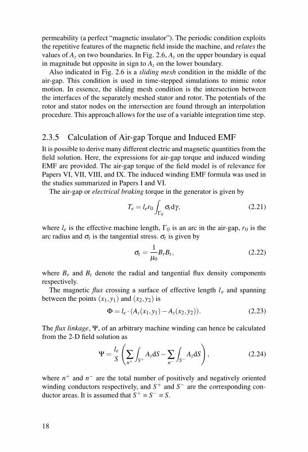
permeability (a perfect “magnetic insulator”). The periodic condition exploitsthe repetitive features of the magnetic field inside the machine, and relates thevalues of Az on two boundaries. In Fig. 2.6, Az on the upper boundary is equalin magnitude but opposite in sign to Az on the lower boundary.

Also indicated in Fig. 2.6 is a sliding mesh condition in the middle of theair-gap. This condition is used in time-stepped simulations to mimic rotormotion. In essence, the sliding mesh condition is the intersection betweenthe interfaces of the separately meshed stator and rotor. The potentials of therotor and stator nodes on the intersection are found through an interpolationprocedure. This approach allows for the use of a variable integration time step.

2.3.5 Calculation of Air-gap Torque and Induced EMFIt is possible to derive many different electric and magnetic quantities from thefield solution. Here, the expressions for air-gap torque and induced windingEMF are provided. The air-gap torque of the field model is of relevance forPapers VI, VII, VIII, and IX. The induced winding EMF formula was used inthe studies summarized in Papers I and VI.

The air-gap or electrical braking torque in the generator is given by

Te = ler0

∫Γ0

σtdγ , (2.21)

where le is the effective machine length, Γ0 is an arc in the air-gap, r0 is thearc radius and σt is the tangential stress. σt is given by

σt =1μ0

BrBt , (2.22)

where Br and Bt denote the radial and tangential flux density componentsrespectively.

The magnetic flux crossing a surface of effective length le and spanningbetween the points (x1,y1) and (x2,y2) is

Φ = le · (Az(x1,y1)−Az(x2,y2)). (2.23)

The flux linkage, Ψ, of an arbitrary machine winding can hence be calculatedfrom the 2-D field solution as

Ψ =leS

(∑n+

∫S+

AzdS−∑n−

∫S−

AzdS

), (2.24)

where n+ and n− are the total number of positively and negatively orientedwinding conductors respectively, and S+ and S− are the corresponding con-ductor areas. It is assumed that S+ = S− = S.

18

The induced winding EMF is derived from the flux linkage as

ew =−dΨdt

. (2.25)

2.4 Coupled Field-circuit ModelsThe conductors in a generator field model are inter-connected to form com-plete windings. The terminals of the field and armature windings are addition-ally connected to external circuits. As the inclusion of conductor subdomainsin windings and circuits affects the conductor currents, additional couplingand circuit equations are required for the field problem to be completely spec-ified in these subdomains.

A model where field and circuit equations are solved simultaneously to pre-dict the behavior of an electric apparatus is usually referred to as a coupledfield-circuit model. This section provides the circuit equations for the coupledfield-circuit models used in the different studies of the thesis. The couplingequations needed to associate a set of conductor subdomains to a winding arealso given.

2.4.1 Coupling Equations for Circuit-connected ConductorsFor a conductor subdomain that is a part of an electric circuit, the field equa-tion (2.17) in that subdomain is supplemented with the following couplingequations

σ∫

Sc

dAz

dtdS−σψc = 0 (2.26)

σψc +Scσ∂Vc

∂ z+ I = 0, (2.27)

where Sc denotes the conductor area,Vc the applied conductor voltage, and I isthe current in the conductor. ψc is the induced conductor EMF integrated overthe conductor surface. The variables I and Vc needs to be determined fromadditional circuit equations, to be presented subsequently.

The structure of (2.26) and (2.27) is the same for all conductor subdomainsthat are connected to circuits, regardless if the conductor is a part of the field,damper or armature winding. The exact formulation of the additional circuitequations for the field, damper and armature windings depends on the studiedproblem, as discussed in the following.

Before the circuit equations are introduced, we state the expression for thetotal electric potential difference across a winding of series-connected con-

19

ductors:

Vw = le

(∑

c∈C +Vc − ∑

c∈C−Vc

). (2.28)

C + here denotes the set of positively oriented conductors, and C − is the setof negatively oriented conductors in the winding.

2.4.2 Rated Voltage No-load Operation ModelRated voltage no-load operation was studied in Papers I, IV and X. Simulationof rated voltage operation at no-load implies consideration of the requirement√

e2a + e2

b + e2c

2= Un, (2.29)

where ea, eb, and ec denote the induced armature phase EMFs and Un is therated line-to-line voltage of the generator. The field voltage is adjusted suchthat (2.29) is met. A short numerical transient is to be expected before theproblem converges.

Field Circuit EquationThe additional circuit equations that complete the problem specification in

field conductor subdomains at rated voltage no-load operation are

u f d0−Vfd = 0 (2.30)

i f+− i f− = 0. (2.31)

u f d0 is the field voltage at no-load operation at rated armature voltage andspeed and Vfd is the potential drop across the entire field winding. Vfdeffectively provides the coupling to (2.17) and (2.26) - (2.27) through (2.28).i f+ and i f− denote the currents in conductor subdomains on opposite sides ofthe pole body. The effects of end winding leakage flux are neglected.

Damper Circuit EquationsThe damper circuit equations are based on a work by Shen and Meunier

[43]. Definitions of relevant quantities are shown in Fig. 2.7. To state the cir-cuit equations on a compact form, the following column vectors are intro-duced:

�i = [i1 i2 ... in]T (2.32)�j = [ j1 j2 ... jn]T (2.33)

�Vb = [Vb1 Vb2 ... Vbn]T (2.34)

�ve = [ve1 ve2 ... ven]T . (2.35)

20

(a)

(b)

Figure 2.7: Damper winding equations in the field model. (a) Definition of bar andend-ring currents. (b) Definition of bar potentials and end-ring voltage drops.

21

Here, the integer n denotes the number of damper bars considered in the cal-culation geometry. For generators with integral slot armature windings,

n =

{2Nd (continuous damper winding)

Nd (non-continuous damper winding),(2.36)

where Nd denotes the number of damper bars per pole.From Fig. 2.7, the following relations can be established between the bar cur-rent vector�i, the end-ring current vector �j, the bar potential vector �Vb and theend-ring voltage vector�ve:

�i = MT�j (2.37)

M�Vb = 2�ve (2.38)

�ve = Red�j. (2.39)

M denotes the (n×n) matrix

M =

⎡⎢⎢⎢⎢⎢⎢⎢⎢⎢⎣

1 −1 0 . . . . . . 0

0 1 −1 0 . . . 0

0 0 1 −1 0 . . ....

... 0 1. . . . . .

......

.... . . . . . . . .

−1 0 . . . . . . 0 1

⎤⎥⎥⎥⎥⎥⎥⎥⎥⎥⎦

(2.40)

and Red denotes the diagonal (n×n) matrix

Red =

⎡⎢⎢⎢⎢⎢⎢⎢⎣

Re1 0 . . . . . . . . .

0 Re2 0 0 . . .... 0

. . . . . . 0...

.... . . . . . 0

0 . . . . . . 0 Ren

⎤⎥⎥⎥⎥⎥⎥⎥⎦

. (2.41)

From (2.37), (2.38), and (2.39), the following relation between�i and �Vb canbe established:

�i =12

MT R−1ed M �Vb (2.42)

Equation (2.42) is the circuit equation that complete the field problem formu-lation in damper conductor subdomains. End-ring leakage flux is neglected.

22

Figure 2.8: Illustration of armature circuit equations during balanced load operation.

2.4.3 Balanced and Unbalanced Load ModelsField models of balanced and unbalanced load generator operation were usedin Paper II.

Field and Damper Circuit EquationsAt balanced and unbalanced load operation, the structure of the field cir-

cuit equation is identical to that of (2.30)-(2.31). In (2.30), the term u f d0 isreplaced by the field voltage required to produce rated armature voltage atthe prescribed load conditions. The field voltage is determined through an it-erative procedure. The initial guess is determined from a magnetostatic fieldsolution, as suggested in [44].

The damper circuit equations during balanced and unbalanced loadoperation are identical to those presented for rated armature voltage no-loadoperation.

Armature Circuit EquationsThe armature circuits at balanced load operation are shown in Fig. 2.8. In

the figure, subindices a, b and c are used to denote the three armature phases.Re and Le denote the end-winding resistance and inductance of an armaturephase, and RL, LL and CL denote resistance, inductance and capacitance of theload. The latter quantities are calculated from the desired active and reactivepower delivery at rated terminal voltage. Further, Rs denotes the resistanceof an armature phase and is implicitly modeled inside the field problem. Thequantities Va,FE , Vb,FE , and Vc,FE finally denote the electric potentials acrossthe armature phases, and are determined according to(2.28). Note that Va,FE ,Vb,FE , and Vc,FE are not the terminal voltages, since they exclude the volt-

23

Figure 2.9: Illustration of armature circuit equations during unbalanced load opera-tion.

age drop across the end-windings. The location of the generator terminals aremarked in the figure.

The circuit equations can be determined from Kirchoff´s circuit laws as:

Va,FE − Reia − Lediadt− RLia − LL

diadt− 1

CL

∫ia dt −

−Vb,FE + Reib + Ledibdt

+ RLib + LLdibdt

+1CL

∫ib dt = 0

(2.43)

Vb,FE − Reib − Ledibdt− RLib − LL

dibdt− 1

CL

∫ib dt−

−Vc,FE + Reic + Ledicdt

+ RLic + LLdicdt

+1

CL

∫ic dt = 0

(2.44)

ia + ib + ic = 0 (2.45)

For simulation of unbalanced load operation, a neutral return is introduced inthe circuit, as shown in Fig. 2.9. Equation (2.45) is then modified accordingto

ia + ib + ic = iN . (2.46)

24

Figure 2.10: Illustration of armature circuits when the generator terminals are con-nected to an infinite busbar.

Furthermore, the loop equation

Vc,FE − Reic − Ledicdt− RLcic − LLc

dicdt− 1

CLc

∫ic dt−

−RNiN − LNdiNdt− 1

CN

∫iN dt = 0

(2.47)

must be added for the problem to be completely specified. Refer to Fig. 2.9for the introduced notation.

2.4.4 Grid-connected FE Model with Mechanical EquationCoupled field-circuit models of grid-connected generators were used in thestudies presented in Papers VII and IX.

Field and Damper Circuit EquationsThe formulation of field and damper winding equations when the generator

is connected to an infinite busbar are identical to those outlined for balancedimpedance load operation.

Armature Circuit EquationsThe armature circuits at grid-connected operation are illustrated in

Fig. 2.10. The sinusoidal voltage sources uBk (k = a,b,c), represent theinfinite bus phase voltages. Transformer and tie-line impedance can beconsidered by introducing supplementary resistive and inductive voltagedrops between the generator terminals and the infinite bus voltage sources.The armature circuit equations with negligible tie-line and transformerimpedance are:

25

Va,FE − Reia − Lediadt−uBa−

−Vb,FE + Reib + Ledibdt

+uBb = 0(2.48)

Vb,FE − Reib − Ledibdt−uBb−

−Vc,FE + Reic + Ledicdt

+uBc = 0(2.49)

ia + ib + ic = 0 (2.50)

Mechanical EquationTo study rotor angle oscillations in a SMIB system, an equation that governs

rotor motion is needed. To this end, the equation

dωm

dt=

1J(Tm−Te), (2.51)

is added. In (2.51), ωm denotes mechanical angular speed, J the moment ofinertia of the rotor, and Tm is the mechanical (drive) torque. The electricaltorque is determined through (2.21).

Problem InitiationA number of different mathematical measures need to be taken in order

to initiate the grid-connected generator field model with a prescribed, steadypoint of operation. The most important actions are:1. The mechanical equation is “de-activated” during the initial numerical tran-

sient by setting J to a very large value. After the field solution has con-verged (typically after ~1-2 electrical periods), J is reset to its actual value.

2. The field current is initially regulated with a proportional controller toquickly obtain the desired power factor. After a few electrical periods, thecontroller is deactivated and the usual, uncontrolled field winding dynamicsis restored.

26

3. Applications of Permeance Modelsof Salient-pole Generators

This chapter reviews the work presented in Papers I, II and III. As statedearlier, the common denominator of these studies is the use of permeancemodels of salient-pole synchronous generators. The permeance model codeimplementation is here described in greater detail and a selection of resultsis discussed. In the review of results from Paper III, only work that entailedcontributions from the author is considered.

3.1 Previous WorkThe construction of the permeance model presented here was primarily in-spired by the works by Traxler-Samek et al. [2] and Knight et al. [45]. Traxler-Samek et al. developed a semi-analytic permeance model intended for use indesign calculations. Among the important features of this model is a statorslot permeance function derived from FE calculations, and the use of an air-gap transformation factor that considers the “bending” of flux tubes of higher-order flux density harmonics [46]. The model presented by Knight et al. alsorelies on permeance functions determined from FEA.

In Paper I, a permeance model is used to determine the effect of the damperwinding on the open-circuit armature voltage waveform of salient-pole syn-chronous generators. The literature holds many studies concerned with thisparticular subject. Walker [47] presented an elaborate theory on the origin andmitigation of problems with slot ripple harmonics. Rocha et al. [48] used ananalytical permeance model combined with damper circuit equations to de-termine the armature voltage harmonic distortion of a salient-pole generator.Keller et al. [49] used a coupled-circuit model derived from stationary FEcalculations to determine armature voltage harmonics of salient-pole gener-ators. In a recent paper, Hargreaves et al. [50] used a coupled-field circuitmodel to predict the effect of damper bar displacement and pole shoe widthon the armature voltage waveform distortion. In both [49] and [50], rotationalperiodicity was utilized to reduce the computation time.

In Paper II, the permeance model is used to predict additional damper wind-ing losses during balanced and unbalanced load operation. Pollard [51] de-rived an analytical expression for the no-load damper loss. Matsuki et al. [52]measured slot ripple frequency damper currents during steady load operation.

27

Knight et al. [53] studied the impact of axial skew and inter-bar contact resis-tance on the damper loss during short-circuit test conditions. Traxler-Sameket al. [46] determined the damper loss in a large hydroelectric generator atshort-circuit test conditions.

In Paper III, the permeance model is used to calculate the UMP in a salient-pole generator with two parallel armature circuits. The use of parallel armaturewinding paths as a means to reduce the resultant UMP in electrical machinesis a topic that has received much attention in the past. A full account of paperson this subject is not provided here. Dorell and Smith [54] used a confor-mal mapping technique to formulate circuit equations that were used to studythe effect of parallel phase bands and equalizer connections on the UMP inan induction motor. Oliveira et al. [55] studied the impact of equipotentialconnections (equalizers) between parallel stator circuits on the UMP in largehydroelectric generators.

3.2 Permeance Model ImplementationA permeance model is based on the underlying principle that the air-gap fluxdensity Bδ can be defined as

Bδ (θm,t) = Λ(θm,t) ·M(θm,t), (3.1)

where Λ denotes an air-gap permeance function and M is the air-gap MMFfunction. θm denotes the mechanical angular coordinate in a stator fixed refer-ence frame and t denotes the time. In the permeance model studied here, theair-gap permeance function is factorized according to

Λ = μ0ΛPΛsatΛSslot . (3.2)

ΛP here denotes the pole shape permeance function, Λsat the saturation per-meance function and ΛSslot the stator slot permeance function. The air-gapMMF function M is the sum of the field (f), the armature (a) and the damperwinding (D) MMF:

M = Mf +Ma +MD. (3.3)

During no-load generator operation, Ma equals zero.

3.2.1 Coordinate SystemThe rotor is assumed to move with the mechanical angular speed ωm in theclockwise direction. At t = 0, a rotor-fixed interpolar axis at the trailing endof a “north” field pole coincides with the stator-fixed coordinate reference.Fig. 3.1 illustrates the stator-fixed coordinate system.

28

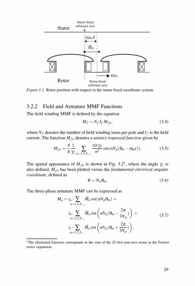
Figure 3.1: Rotor position with respect to the stator-fixed coordinate system.

3.2.2 Field and Armature MMF FunctionsThe field winding MMF is defined by the equation

Mf = Nf I f Mfn, (3.4)

where Nf denotes the number of field winding turns per pole and I f is the fieldcurrent. The function Mfn denotes a unitary trapezoid function given by

Mfn =4π

1γ f

∑n=1,3,5,...

sinγ f

n2 sin(nNp(θm−ωmt)). (3.5)

The spatial appearance of Mfn is shown in Fig. 3.21, where the angle γ f isalso defined. Mfn has been plotted versus the fundamental electrical angularcoordinate, defined as

θ = Npθm. (3.6)

The three-phase armature MMF can be expressed as

Ma = ia · ∑n=1,3,5,...

Mn sin(nNpθm) +

ib · ∑n=1,3,5,...

Mn sin

(nNp(θm− 2π

3Np))

+

ic · ∑n=1,3,5,...

Mn sin

(nNp(θm +

2π3Np

))

,

(3.7)

1The illustrated function corresponds to the sum of the 25 first non-zero terms in the Fourierseries expansion.

29

0 30 60 90 120 150 180 210 240 270 300 330 360−1.2

−1−0.8−0.6−0.4−0.2

00.20.40.60.8

11.2

Electrical angle, θ (°)

Uni

tary

fie

ld M

MF

func

tion

γf

Figure 3.2: Unitary trapezoid function (used to model the field winding MMF).

0 30 60 90 120 150 180 210 240 270 300 330 360−1.2

−1−0.8−0.6−0.4−0.2

00.20.40.60.8

11.2

Electrical angle, θ (°)

Uni

tary

arm

atur

e M

MF

func

tion

Figure 3.3: Unitary three-phase armature MMF function.

where ia, ib, and ic denote the currents in the winding phases A, B, and Crespectively. The coefficients Mn are given by

Mn =4π

Ns

2Np

1nkd(n)kp(n)ksl(n), (3.8)

where Ns denotes the total number of winding turns per phase circuit. Ex-pressions for the distribution, pitch and slot opening factors (symbols kd(n),kp(n), and ksl(n) respectively), can be found in [56]. Fig. 3.3 shows the spatialappearance of a normalized three-phase armature MMF function for balancedfundamental three-phase current supply.

30

0 30 60 90 120 150 180 210 240 270 300 330 3600

5

10

15

20

25

30

35

40

45

50

Electrical angle, θ (°)

Pole

sha

pe p

erm

eanc

e fu

nctio

n (m

−1 )

Figure 3.4: Pole shape permeance function of Generator I in Paper I.

3.2.3 Pole Shape Permeance FunctionThe pole shape permeance, ΛP, is determined from a stationary FEAaccording to the following procedure:

1. The geometry corresponding to one pole pitch of studied generator topol-ogy is created in the FE software.

2. Rotor and stator regions are assigned with linear magnetic properties andhigh relative permeability (μr = 10000).

3. Stator and damper slot regions are assigned with linear magnetic propertiesand high relative permeability (μr = 10000).

4. The air-gap flux density waveform resulting from field winding excitationis sampled along a line in the air-gap. This waveform is denoted Blinear .

5. ΛP is obtained by dividing Blinear with Mf . To avoid division with zero,the functional values of ΛP close to the inter-polar gaps are determinedthrough linear extrapolation.

Fig. 3.4 shows the pole shape permeance function of Generator I from Paper I.Notice the peculiar appearance near the pole shoe tips, located close to theangles 40◦, 140◦, 220◦ and 320◦.

3.2.4 Saturation and Stator Slot Permeance FunctionsThe determination of the saturation and slot permeance functions is a chal-lenging task. The saturation permeance is, in part, a result of the saturation inthe stator teeth. Hence, from a physical point of view, it is difficult to motivatea separation of the slot and saturation permeance functions.

31

In the mathematical description of the permeance model, the separation isnevertheless necessary. The reason for this is that the permeance variationsdue to stator slotting is a stator-fixed phenomenon, while the saturation “pro-file” should move along with the revolving fields. The mathematical treatmenttherefore becomes overly complicated unless a factorization according to (3.2)is carried out.

The author tested different methods to determine Λsat and ΛSslot . Thecomputational procedure presented next was found to give the best results.

Determination of Λsat

1. The generator geometry is created in a FE software.2. Rotor and stator regions are assigned with non-linear magnetic properties.3. The flux density waveform resulting from field excitation (no-load study)

or a combination of armature and field excitation (load study) is sampledalong a line in the air-gap. This waveform is denoted Breal .

4. The ratio Λcomb = Breal/Blinear is calculated. Blinear here denotes the fluxdensity wave used in the extraction of the pole shape permeance function.Λcomb can be regarded as a relative permeance function that holds the com-bined effects of saturation and stator slotting.

5. The discrete Fourier series expansion of the function 1/Λcomb is calculated.Contributions from space harmonics of orders 6nq1± 1 (n = 1,2 . . .) arethen subtracted from this function (q1 denotes the number of stator slotsper pole and phase). The result is re-inversed and is denoted Λ sat .

6. Linear extrapolation is used to smooth the function near the inter-polargaps.

Determination of ΛSslot1. One slot pitch of the function Λcomb close to the pole axis is extracted (see

Fig. 3.5).2. The discrete Fourier series expansion of the extracted portion of Λcomb is

used to build the function ΛSslot according to the structure of Eq. (6) inPaper I.

3. ΛSslot is finally normalized such that its maximum value equals one.Accordingly, Λsat must be multiplied with the same normalization factorin order to preserve the requirement that Λcomb = ΛsatΛSslot .

Figs. 3.6-3.7 illustrate the saturation and stator slot permeance functions ofGenerator I from Paper I, calculated for no-load operation at rated field cur-rent.

32

Figure 3.5: Combined saturation and stator slot permeance function of Generator I inPaper I at rated no-load operation. The permeance function is illustrated at t = 0.

0 30 60 90 120 150 180 210 240 270 300 330 3600

0.2

0.4

0.6

0.8

1

1.2

Electrical angle, θ (°)

Satu

ratio

n pe

rmea

nce

func

tion

Figure 3.6: Saturation permeance function of Generator I in Paper I at rated no-loadoperation. The permeance function is given at t = 0.

3.3 Damper Winding MMF and Circuit EquationsThe product of the air-gap permeance and the sum of the field and armatureMMFs typically result in waveform with a high harmonic contents. Accord-ing to Lenz’s law, any space harmonic that move with respect to the rotor willinduce EMFs in conductors installed on the rotor. If the conductors are partof closed circuits, a flow of electric current will result. These reaction cur-rents introduce an additional MMF component that must be considered in thecalculation of the air-gap flux density.

The permeance model presented here considers induced currents in thedamper winding, but not in the field winding. This simplification is motivated

33

0 30 60 90 120 150 180 210 240 270 300 330 3600

0.2

0.4

0.6

0.8

1

1.2

Electrical angle, θ (°)

Stat

or s

lot p

erm

eanc

e fu

nctio

n

Figure 3.7: Stator slot permeance function of Generator I in Paper I at rated no-loadoperation.

by the limited depth of penetration of air-gap flux density harmonics into thepole shoe. Since the damper winding is located closer to the air-gap than thefield winding, the damper reaction also has a decidedly greater impact on theair-gap flux density waveform.

The damper MMF is determined from the flux density waveform set up bythe sum of the field and armature MMFs. The damper MMF contribution isthen added to the original air-gap flux density wave. The saturation permeanceis assumed to be unaffected by the supplementary magnetic flux introduced bythe damper MMF.

3.3.1 Flux Density HarmonicsBelow, air-gap flux density harmonics that introduce damper windingcurrents and are considered in the permeance model are briefly described.

Slot Harmonic WavesThe interaction between the stator slot permeance function and the fun-

damental MMF wave gives rise to the following series of flux density wavepairs:

∑n=1,2,...

B+n cos((nQs +Np)βm +nQsωmt)−

∑n=1,2,...

B−n cos((nQs−Np)βm +nQsωmt).(3.9)

In (3.9),βm = θm−ωmt (3.10)

34

is a rotor-fixed angular coordinate, and Qs denotes the total number of statorslots. The waves of (3.9) travel with linear speeds

vn =− 6q1n6q1n±1

ωτp

π(3.11)

with respect to the rotor, and induce EMFs of angular frequencies

ωn = n6q1ω (n = 1,2, . . .) (3.12)

in the damper winding. Here, ω = Npωm denotes the fundamental electricalangular frequency, q1 is the number of stator slots per pole and phase and τ p

denotes the pole pitch.

Armature MMF Space HarmonicsIn addition to the fundamental wave, a balanced three-phase armature MMF

gives rise to the following series of space harmonics:

∑n=5,11,...

Bncos(nNp(θm +ωmtn

) +

∑n=7,13,...

Bncos(nNp(θm− ωmtn

).(3.13)

The waves travel with linear speeds

vn =−τp

πn±1

nω (3.14)

with respect to the rotor. The + sign refers to harmonic orders n = 5,11, . . .,while the − sign refers to harmonic orders n = 7,13, . . .. It can be shown thatthese waves induce EMFs of angular frequencies

ωn =

{(n+1)ω n = 5,11, . . .

(n−1)ω n = 7,13, . . .(3.15)

in the damper winding. Hence, the wave-pair n = 5,7 induce sinusoidalEMFs of frequency 6ω , the wave-pair n = 11,13 induce EMFs of frequency12ω , and so forth.

Fundamental Negative Sequence HarmonicUnbalanced steady load operation gives rise to a fundamental space har-

monic that rotates backwards. This wave travels with linear speed

v2 =−2τp

πω (3.16)

35

Figure 3.8: Definition of a damper loop and the corresponding loop current.

with respect to the rotor, and induces EMFs of frequency

ω2 = 2ω (3.17)

in the damper winding.

3.3.2 Unitary Damper Loop MMF FunctionsEach damper bar is considered to be a part of two adjacent damper loops, asillustrated in Fig. 3.8. When the current ik flows in loop k, its effect on theair-gap flux density is considered through a damper loop MMF

MDk(θ ,t) = ik(t)MDk0(θ ,t), (3.18)

where MDk0 denotes the unitary MMF function of loop k. When symmetryconditions allow for a reduction of the calculation geometry to two fundamen-tal pole pitches, the unitary loop MMF function is conventionally modeled asshown in Fig. 3.9. In the figure, the rising and falling flanks of the curve markthe positions of the loop conductors.

The unitary loop MMF function of Fig. 3.9 is a normalized square-functionwith a duty cycle determined by the ratio of the electrical damper loop spanand a full fundamental electrical period. The function is shifted upwards suchthat the condition ∫ 2π

0MDk0(θ )dθ = 0 (3.19)

is fulfilled. For a loop current ik �= 0, this conventional unitary loop MMFfunction predicts uniform air-gap flux density outside the angular span di-rectly in front of the loop. Physically, this is however unrealistic. The onlyflux lines that actually cross the air-gap, and therefore affects the air-gap fluxdensity waveform, are situated directly in front of the damper loop, as illus-trated in Fig. 3.10. Thus, as far as the flux crossing the air-gap radially isconcerned, a more appropriate unitary loop MMF function is the one illus-trated in Fig. 3.11. In this modified function, the MMF is effectively set to

36

0 30 60 90 120 150 180 210 240 270 300 330 360−0.2

0

0.2

0.4

0.6

0.8

1

Electrical angle, θ (°)

Cla

ssic

al u

nita

ry lo

op M

MF

func

tion

Figure 3.9: The classical unitary damper loop MMF function.

Figure 3.10: Flux line distribution upon excitation of a single damper loop.

zero outside the angular span of the damper loop, as this region does containvery few radial flux lines that cross the air-gap.

For reasons of symmetry, the currents in damper loops that are identicallypositioned on adjacent poles approximately become equal in magnitude and180◦ out of phase. Hence, it may be argued that the condition (3.19) is ap-proximately met even after the adoption of the modified unitary loop MMFdefinition, provided that the MMF contributions from these loops are consid-ered together.

The modified unitary damper loop MMF function was adopted in the stud-ies presented in this thesis.

3.3.3 Calculation of Damper Loop CurrentsThe damper loop currents are calculated from circuit equations derived fromKirchoff’s voltage law. One set of equations is formulated for every angular

37

0 30 60 90 120 150 180 210 240 270 300 330 360−0.2

0

0.2

0.4

0.6

0.8

1

Electrical angle, θ (°)

Mod

ifie

d un

itary

loop

MM

F fu

nctio

n

Figure 3.11: Modified unitary damper loop MMF function.

frequency that exist in the damper winding for a given case study (no-load,balanced load, or unbalanced load operation). The total loop currents are thenobtained through addition of the loop current harmonics.

For the frequency ωn, the circuit equations can be compactly written as

U= ZlIl + jωnMIl. (3.20)

U here denotes a column vector that holds the induced loop EMFs, Zl isthe loop impedance matrix, M is the mutual loop inductance matrix and Ilis a column vector whose elements correspond to the loop currents. Whengenerators with integral slot armature windings are analyzed, it is sufficient tostudy two pole pitches of the air-gap. In this case, U and Il become (2Nd×1)vectors and Zl andM become (2Nd×2Nd) matrices.

Induced Loop EMF VectorU contains the induced loop EMFs of frequency ωn. An induced loop EMF

is here defined as the sum of the EMFs that are induced in the damper barsthat constitute the loop, added with appropriate signs. Complex notation isintroduced to represent the loop EMFs according to

U=

⎛⎜⎜⎜⎜⎝

U1

U2...

UN

⎞⎟⎟⎟⎟⎠ =

⎛⎜⎜⎜⎜⎝

U1e jα1

U2e jα2

...

UNe jαN

⎞⎟⎟⎟⎟⎠ . (3.21)

N here denotes the total number of damper loops in the calculation geometry.The complex EMFs Uk (k = 1,2, . . . ,N) are composed of the vector sum of

38

all the EMFs induced by flux density space harmonics that contribute to therotor frequency ωn.

The amplitude of the bar EMF component introduced by the m-th flux den-sity space harmonic that contribute to the frequency ωn is determined throughthe flux cutting EMF equation as

Ubn,m = lb vn,m Bn,m. (3.22)

lb here denotes the length of the damper bar and vn,m is the linear speed of them-th space harmonic with respect to the rotor. The flux density amplitude Bn,m

is estimated from a Fourier series expansion of the flux density wave

Bδ (θm,t = 0) = Λ(θm,t = 0) · [Mf (θm,t = 0)+Ma(θm,t = 0)], (3.23)

and is subsequently modulated with a flux reduction coefficient that compen-sates for the decrement in radial harmonic flux from the middle of the air-gapto the damper cage, located below the pole face. The flux reduction coeffi-cients were determined from a series of magnetostatic FE calculations and,seemingly, serve the same purpose as the air-gap transformation factor pre-sented in [46].

Consideration of the location of the positive peaks of the exciting spaceharmonics with respect to the damper bar positions provide the appropriatephase shifts αk (k = 1,2, . . . ,N).

Loop Impedance MatrixThe matrix Zl is given by

Zl =

⎡⎢⎢⎢⎢⎢⎢⎢⎢⎢⎢⎢⎣

Z′1 −Zb 0 . . . 0 −Zb

−Zb Z′2 −Zb

. . . . . . 0

0. . . . . . . . . . . .

......

. . . −Zb Z′k −Zb

. . .

0. . . . . . . . . . . . . . .

−Zb 0. . . . . . −Zb Z

′N

⎤⎥⎥⎥⎥⎥⎥⎥⎥⎥⎥⎥⎦

. (3.24)

In the expression above, Zb denotes the bar impedance. Analytical expressionspresented in [57] were used to determine the AC resistances and leakage in-

ductances of the damper bars. The impedances on the main diagonal, Z′k , are

given by

Z′k = 2(Zb +Zek), (3.25)

39

where Zek denotes the end-ring impedance of the k-th damper loop. End-ringdamper impedances were estimated with expressions from [58].

Mutual Loop Inductance MatrixAs indicated in Fig. 3.10, the most important flux couplings occur between

the closest neighboring damper loops. These mutual flux paths are moreovercharacterized by the permeances normally associated with slot and tooth tipleakage flux. Based on these observations, it was decided that only the mutualcoupling between adjacent damper loops were to be considered in the model.Furthermore, the magnitude of the mutual inductance between two adjacentdamper loops was set to

MDD = Lso +Ltt , (3.26)

where Lso denotes the damper slot opening leakage inductance and Ltt denotesthe tooth tip leakage inductance. The self inductance of loop k was similarlydefined as

Lkk = 2 · (Lso +Ltt)+LmDk, (3.27)

where LmDk denotes the main loop inductance. LmDk was determined by aver-aging the air-gap permeance in front of the k-th damper loop.

With the introduced notation, the matrix M is formulated as

M=

⎡⎢⎢⎢⎢⎢⎢⎢⎢⎢⎢⎢⎣

L11 −MDD 0 . . . 0 −MDD

−MDD L22 −MDD. . . . . . 0

0. . . . . . . . . . . .

......

. . . −MDD Lkk −MDD. . .

0. . . . . . . . . . . . . . .

−MDD 0. . . . . . −MDD LNN

⎤⎥⎥⎥⎥⎥⎥⎥⎥⎥⎥⎥⎦

. (3.28)

3.3.4 Resultant Damper MMFAdopting a cosine reference, a complex damper loop current of frequencyωn and determined through (3.20) is transformed into a real-valued functionaccording to

Ik,n = Ikejϕk ⇒ ik,n(t) = Ikcos(ωnt +ϕk). (3.29)

The resultant damper winding MMF is then calculated as

MD =N

∑k=1

(∑n

ik,n(t))

MDk0(θ ,t). (3.30)

40

Figure 3.12: THD of the open-circuit armature voltage waveform of Generator I inPaper I. The damper winding is continuous with six damper bars per pole, and iscentered around the pole axis.

3.4 Selected Results3.4.1 THD of the Open-circuit Armature Voltage WaveformIn Paper I, the permeance model was used to determine the harmonic contentsin the open-circuit armature voltage waveform of large hydroelectric gener-ators. Particular attention was devoted to the impact of the damper windingreaction on the so called slot ripple harmonics. Slot ripple voltage harmonicsare produced by the damper MMF induced by the stator slot harmonic fluxdensity wave-pairs in (3.9). They correspond to the harmonic frequencies

ωslot = 6nq1±1 n = 1,2, . . . (3.31)

Fig. 3.12 shows the calculated Total Harmonic Distortion2 (THD) of the open-circuit armature voltage versus the damper slot pitch (τds) for one of the stud-ied generator topologies. The damper slot pitch is stated as a fraction of thestator slot pitch. In the figure, THD predictions obtained with the permeancemodel are compared to those obtained with a FE model. The damper windingin the studied unit is a continuous winding with six equidistant damper barsper pole, centered around the pole axis.

The THD essentially reflects the stator slot harmonic contents in the voltagewaveform, and is seen to be maximal for τds = 1. This is in line with the theorypresented in [59]. Moreover, it is observed that the THD predictions of the twomodels are very close.

Further numerical experiments with the permeance model revealed that theTHD vs. τds - profile typically is highly susceptible to the resistance of theelectrical connection between the damper cages on adjacent poles, Rc. This

2The THD is defined in (19) of Paper I.

41

Figure 3.13: THD versus damper slot pitch for different values of the inter-pole cou-pling resistance, Rc.

feature is illustrated in Fig. 3.13, where THD vs. τds - profiles are providedfor three different Rc-values. The basic damper winding configuration is thesame as that described in conjunction with Fig. 3.12 (six equidistant centeredbars).

A highly resistive inter-pole coupling corresponds to a grill winding, whilea low Rc-value corresponds to a complete squirrel-cage. Fig. 3.13 indicatesthat if the objective is to reduce the slot ripple voltage harmonic contents byan appropriate choice of damper slot pitch, the optimal choice will effectivelydepend on the basic damper winding configuration (grill or complete squirrel-cage).

3.4.2 Damper Bar Currents at Rated Load OperationFig. 3.14 shows the calculated first phase belt harmonic damper bar currents3

in a large hydroelectric generator at rated load operation. The studied damperwinding is continuous, with seven bars per pole. Bar 1 is located on the trailingside of the pole. In the figure, permeance model data is compared with theresults from FE calculations.

The bar current predictions are in fair, but not excellent agreement. Thelargest discrepancies are observed in the outermost bars.

3These current harmonics are introduced by MMF armature harmonics of orders 5 and 7.

42

Figure 3.14: Calculated RMS values of first phase belt frequency (360 Hz) damperbar currents in the test generator of Paper II.

3.4.3 Reduction of the UMP by Parallel Armature CircuitsIn permeance models, stationary off-centered rotor operation can be modeledby modulating the air-gap permeance with a function

Λecc =1

1− ε · cos(θm−α), (3.32)

where ε denotes the relative rotor eccentricity, and α is the position of theminimum air-gap length with respect to the angular coordinate origin. Theuneven air-gap length around the rotor periphery leads to increased flux den-sity levels where the air-gap is shorter, and decreased flux density levels on theside where the air-gap is longer. This uneven air-gap flux density profile givesrise to a magnetic force resultant termed unbalanced magnetic pull (UMP).

In synchronous generators with more than one circuit per armature phase,the asymmetric air-gap introduces currents that circulate between the parallelcircuits both during no-load and load operation. The MMF set up by these cur-rents counteracts the air-gap flux density wave modulation, and, accordingly,reduces the UMP.

In Paper III, a simple extension of the permeance model that allowed forthe consideration of currents circulating between parallel armature windingphases was examined. Fig. 3.15 illustrates the air-gap flux density profile in atwelve-pole synchronous machine operating at no-load, before and after addi-tion of the circulating armature current MMF.

As can be expected, the calculated armature MMF to some extent “evensout” the air-gap flux density waveform. Thus, the validity of the suggestedmodeling principle of this phenomenon is, at least qualitatively, confirmed.

43

Figure 3.15: No-load air-gap flux density waveforms in the test generator of Paper IIIwith 24% relative static eccentricity, calculated with the permeance model. The rotoris displaced toward the “middle point” of one phase circuit group and the applied fieldcurrent equals 30 A. The stator slot permeance was omitted from the analysis.

44

4. Core Loss Prediction in LargeHydroelectric Generators

This chapter reviews the work presented in Paper IV. A brief background onpractical iron loss estimation is also provided.

4.1 Previous WorkThe technical literature contains a vast amount of papers on the subject of ironlosses in electrical machines. Here, only a very limited number of works withemphasis on iron loss modeling and rotational core losses are mentioned.

Fiorillo and Novikov [60] derived formulae for the calculation of the aver-age iron loss in magnetic steel laminations, applicable for arbitrary periodicflux density waveforms. Moses [61] measured the locus of the magnetic fluxdensity vector in the core of rotating machines and identified regions wherebidirectional flux is prominent. Stranges and Findlay [6] tested different lossprediction schemes on the field solutions obtained from FEA of inductionmachines. Experimental loss curves for various axis ratios were used to ac-count for flux density bidirectionality. Bottauscio et al. [3] compared post-processing and vector hysteresis iron loss evaluation techniques on field so-lutions obtained from FEA. Díaz et al. [10] presented analytical formulae forrotational loss prediction in induction machines. The study concluded that itwas sufficient to consider rotational losses only in a region near the statortooth roots.

4.2 Iron Loss Estimation4.2.1 Loss SeparationThe total instantaneous specific power loss in steel laminations is usuallyconsidered to be constituted of three parts; the hysteresis loss (1), the clas-sical eddy current loss (2) and the excess loss (3). The decomposition of theloss into three distinct terms is called loss separation. Physically, this conceptemerges as a result of magnetization reversal processes that occur on differentspatial scales [62].

45

The time average of the total specific power loss in magnetic steel sheetsexposed to sinusoidal flux density of peak value Bmax and frequency f is con-ventionally modeled as

ptot = kH fB2max + kc f 2B2

max + kE f 1.5B1.5max. (4.1)

Here, the first term represents the hysteresis loss, the second term is the classi-cal loss, and the last term is the excess loss. The coefficient kc is the classicalloss coefficient

kc =π2σd2

6ρm, (4.2)

where σ denotes the electric conductivity, d the thickness, and ρm the massdensity of the steel laminate. The loss coefficients kH and kE are typicallydetermined through curve fitting of measured loss data.

Equation (4.1) corresponds to a frequency domain model, and rigorouslyonly applies for sinusoidal excitation. The model can be re-formulated as atime domain model according to

ptot = kH fB2max +

k′c

T

∫ T

0

∣∣∣∣dBdt

∣∣∣∣2

dt +k′E

T

∫ T

0

∣∣∣∣dBdt

∣∣∣∣1.5

dt, (4.3)

where B denotes the flux density vector and T = 1/ f is the excitation pe-riod. Equation (4.3) can be used to estimate the iron loss of any periodic fluxdensity waveform, provided its frequency is close to f . In some situations,empirical corrections for the loss associated with minor loop flux reversalscan be motivated [63].

The modified loss coefficients k′c and k

′E are equal to

k′c =

kc

2π2 , (4.4)

and

k′E =

kE√2π

∫ 2π0 |cosx|1.5 dx

, (4.5)

and are determined such that (4.3) yields the same result as (4.1) for the specialcase of sinusoidal excitation.

4.2.2 Rotational LossesThe loss separation formulae introduced in the previous section are valid ifthe time-varying flux density oscillates in one distinct direction. Such a fluxdensity vector is here referred to as an alternating quantity. In electrical ma-chines, the flux density in some regions of the stator core is however stronglybidirectional. That is, the locus traced by the tip of the flux density vector

46

Figure 4.1: Definition of Bmax and Bmin in the spatial locus of a time-periodic fluxdensity vector. xy is an arbitrary Cartesian coordinate system.

Figure 4.2: Measured ratio between the power loss at purely rotational conditionsand the power loss at purely alternating conditions. The curve was derived from datapresented in [6]. The test material was a 0.47 mm SiFe steel with 2.7% silicon content.

during a full electrical period resembles an ellipse rather than a straight line.Regions with bidirectional flux density are said to be exposed to rotationalflux.

The degree of rotation of the flux density waveform is determined by thefundamental axis ratio, Γ, of the locus traced by the tip of the flux densityvector during a complete excitation period. Here, the fundamental axis ratioof an arbitrary locus is approximated by

Γ =Bmin

Bmax, (4.6)

where the reader is referred to Fig. 4.1 for a definition of Bmin and Bmax.For identical excitation frequency and amplitude, the power loss associ-

ated with exposure to flux density of a non-zero degree of rotation typicallyis higher than the loss at purely alternating conditions. The ratio between thepower loss at purely rotating conditions (Γ = 1) and purely alternating condi-tions (Γ = 0) typically depends on Bmax, as illustrated in Fig. 4.2.

47

Iron loss prediction models may be adjusted for the influence of these “ro-tational losses” in various ways. The frequency domain model (4.1) may forinstance be modified according to

ptot = (1+δΓ) · (kHB2max f + kcB

2max f 2 + kEB1.5

max f 1.5), (4.7)

where the factor δ is a weighting factor that determines the specific loss in-crease attributable to flux rotation. Equation (4.7) effectively determines thespecific loss associated with an arbitrary elliptical flux density locus throughlinear interpolation between a purely alternating and a purely rotating loss.The modification was originally proposed by Ma et al. [5].

For the time-domain model (4.3), a detailed consideration of rotational ef-fects results in the following modified expression [64]

ptot = ((1−Γ)+Γ ·RH(Bmax))kHB2max f +

k′c

T

∫ T

0

∣∣∣∣dBdt

∣∣∣∣2

dt

+ ((1−Γ)+Γ ·RE(Bmax))k′E

T

∫ T

0

∣∣∣∣dBdt

∣∣∣∣1.5

dt. (4.8)

Again, a weighted interpolation technique between purely alternating andpurely rotating losses is adopted, but contrary to (4.7), the interpolation isperformed on the individual loss components. In (4.8), the function RH(Bmax)represents the ratio between the purely rotational and the purely alternatinghysteresis loss and RE(Bmax) is the ratio between the purely rotational and thepurely alternating excess loss. These functions can be obtained by applying athree-term loss decomposition scheme on measured specific loss data [64].

The functions RH(Bmax) and RE(Bmax) typically display strong qualitativeresemblance [60,64]. For instance, they both decrease monotonically and dropto zero at high flux density levels.

4.3 Study SummaryNo-load operation of twelve large hydropower generators denoted I - XII wassimulated with a 2-D time-stepped FE model. From the calculated magneticflux density distributions, the no-load core losses were estimated with threedifferent loss prediction models, denoted A, B and C. Information about thestudied units can be found in Table II, Paper IV.

Model AModel A, referred to as the alternating loss model, evaluated the specific coreloss with (4.1). The constant loss coefficients kH and kE were obtained frommultivariate curve fitting of the lamination manufacturer’s loss data recorded

48

Figure 4.3: Assumed ratio between the rotational and alternating hysteresis loss in thecore materials. The curve is derived from data presented by Bottauscio et al. [3].

at 50, 100 and 200 Hz.

Model BModel B assessed the specific core loss through (4.7). The weighting factorδ was set to the constant value 0.6. This implies that the model predicts aspecific loss density that is 60 % higher for Γ = 1 compared to when Γ = 0,independently of Bmax. This is a fair estimate for flux density levels on theorder of 1-1.6 Tesla, but will lead to an underestimation of the additionalrotational loss at low flux density levels [6]. The loss coefficients are thesame as those used in Model A.

Model CModel C assessed the specific core loss through (4.8). Because rotational lossdata were not available for the studied core materials, a rotational hystere-sis loss curve considered “typical” for non-oriented SiFe-laminations used inelectrical machines was used to model the function RH . RE was further as-sumed to be identical to RH . The employed curve was derived from [3] and isprovided in Fig. 4.3.

In order to assess the influence of flux bidirectionality on the calculated coreloss, the total core loss figures obtained with Models B and C were comparedwith the total core loss figure obtained with Model A. If the total core lossestimate obtained with Model A is termed PA

tot , and PBtot denotes the core loss

obtained with Model B, then the fractional core loss increase attributable torotational effects as predicted by Model B can be evaluated as

Padd−rot = 100 ·(

PBtot−PA

tot

PAtot

)[%]. (4.9)

49

Figure 4.4: Core losses predicted by Models A, B, and C. The loss figures are pre-sented in % of the measured electromagnetic no-load loss.

Similarly, the difference between the core loss calculated with Model C, PCtot ,

and the loss PAtot ,

Padd−dyn = 100 ·(

PCtot−PA

tot

PAtot

)[%], (4.10)

is a measure of the combined importance of harmonics and rotational effectson the total core loss estimate.

4.4 Selected ResultsThe calculated core losses for the twelve generators, as predicted by ModelsA, B, and C are shown in Fig. 4.4. Observe that the lines between the datapoints merely serve as “guides for the eye”. The loss figures are presented in% of the measured electromagnetic no-load loss.

Model A consistently yielded the smallest loss predictions, with an the av-erage of about 51% of the measured loss. Model C, that takes the influence ofharmonics and rotational effects into account, yielded the highest loss predic-tions, with an average of 65% of the measured loss. Hence, additional straylosses, model inaccuracies and measurement errors are indirectly predictedto account for 35% of the total electromagnetic no-load loss. The significantspread in the discrepancy between calculated and measured loss figures be-tween the different machines suggests that differences in machine design phi-losophy, which in turn determine the magnitude of the stray losses, have adecisive impact on this type of loss comparisons.

50

Figure 4.5: Degree of rotation in the core of Generator XII during no-load operation.Γ = 0 (blue) signifies purely alternating flux while Γ = 1 means purely rotational flux.

Figure 4.6: Padd−dyn = loss increase attributable to dynamic effects (flux rotation +harmonic distortion), as predicted by Model C. Padd−rot = loss increase attributable toflux rotation, as predicted by Model B.

Fig. 4.5 shows the calculated degree of rotation in the core of Generator XIIduring no-load operation. The highest degree of rotation is found in the statorteeth roots and typically amounted to about 0.7-0.8 in the studied generators.More than 50% of the yoke is exposed to fields with a degree of rotation higherthan 0.3. The flux in the teeth is nearly purely alternating.

The effect of harmonics and flux rotation on the calculated core losses isillustrated in Fig. 4.6. The rotational loss correction predicted by Model B(Padd−rot) varied between 10 and 18% for the studied generators, the averagebeing 13%. The fractional loss increase Padd−dyn, which takes both harmonicand rotational effects into account, varied between 11 and 50% and was 28%on the average. The major part of this loss increase is attributable to rotationaleffects.

51

The exceptionally high loss increase caused by dynamic effects in Gener-ator I is due to low flux density levels in the over-dimensioned stator core ofthis machine. At low flux density levels, the rotational loss correction is sub-stantial (see Fig 4.3), and hence the fractional loss increase Padd−dyn becomesvery pronounced.

52

5. Form Factors of Salient Pole Shoes

This chapter reviews the work presented in Paper V.

5.1 BackgroundThe study on salient pole shoes started in parallel with the author’s elaborationof a computer program for the analytic determination of the main inductancesof salient-pole synchronous machines. In analytic calculations, the direct (d),quadrature (q) and field ( f ) magnetizing inductances are determined as

Xjm ∝ k j Xm ( j = d,q, f ) , (5.1)

where Xm denotes the main armature inductance of a machine with constantair-gap length, and k j is the form factor for excitation type i1. The form factorsare scalars that take the combined effects of the air-gap permeance and MMFwaveforms into account.

To assist in the determination of pole shoe form factors, many textbookscite a classical paper by Wieseman [14]. In that study, a graphical method isused to characterize a large number of pole shoe shapes. Curves for the deter-mination of form factors of arbitrary pole shoe geometries are also presented.

In order to assess the accuracy of the curves presented in [14], we comparedthe output from Wieseman’s form factor formulae to data extracted from FEcalculations. It was deduced that for certain pole shoe geometries and excita-tion levels, Weiseman’s form factors deviated with about 10-20% from the FEdata.

The work presented in Paper V had two main objectives. The firstobjective was to derive accurate form factors for the salient-pole generatortopologies studied in Papers VII-VIII. The second objective was to conduct acomprehensive study on the subject of pole shoe form factors, as a modernreview of Wieseman’s work. The intention with the latter study was toprovide updated data that can assist machine designers in the selection of thepole shoe shape.

With Wieseman’s study as a point of departure, two aspects were given specialattention:

1Some authors also refer to these constants as flux distribution coefficients.

53

Figure 5.1: Air-gap flux density waveform, Bgd(θ), set up by armature excitationalong the pole (d-) axis. Bgd1(θ) is the fundamental wave.

1. The effect of iron saturation on the pole shoe form factors. Weiseman’sstudy is based on the assumption of infinite relative permeability in therotor and stator. The impact of saturation on the form factors is therefore ofinterest.

2. The extent to which the details of the pole face contour affect the formfactors. Weiseman’s form factors are determined through a very limited setof parameters that characterizes the geometry of the pole shoe.

5.2 Pole Shoe Form FactorsDirect Axis Armature Pole Shoe Form Factor

The direct axis armature pole shoe form factor kd is determined from theair-gap flux density waveform produced by a sinusoidal armature MMF actingdirectly in front of the pole axis. This excitation results in a slightly peakedwaveform, as shown in Fig. 5.1. kd is defined as

kd =Bgd1

Bgdm, (5.2)

where Bgd1 is the amplitude of the fundamental and Bgdm is the peak value ofthe flux density waveform.

Quadrature Axis Armature Pole Shoe Form FactorThe impression of sinusoidal armature MMF in front of the pole-gap

(quadrature) axis, produces an air-gap flux density wave whose qualitativeappearance is illustrated in Fig. 5.2. The quadrature axis armature pole shoe

54

Figure 5.2: Air-gap flux density waveform, Bgq(θ) set up by q-axis armature excita-tion. Bgq1(θ) is the fundamental wave.

form factor is here defined as2

kq =Bgq1

Bgd1, (5.3)

where Bgq1 denotes the amplitude of the fundamental of the waveform Bgq(θ )and Bgd1 is the fundamental of the waveform set up by excitation along thedirect axis. kq is a direct measure of the ratio Xqm/Xdm.

Field Winding Pole Shoe Form FactorField winding excitation results in a flat-topped air-gap flux density wave-

form, as illustrated in Fig. 5.3. In analogy with the previous definitions, thefield winding pole shoe form factor k f is defined as

k f =Bg f 1

Bg fm. (5.4)

Bg f 1 is the amplitude of the fundamental and Bg fm is the peak value of theresulting wave.

5.3 Study SummaryThe pole shoe form factors kd , kq, and k f of a large number of salient poleswere determined from air-gap flux density waves obtained in 2-D magneto-static FE calculations. Additionally, the THD of the air-gap flux density wavesproduced by field winding excitation was determined, since this is a traditionalmeasure of the harmonic “imprint” of the pole shoe.

2The definition is different from the one used in [14]. The employment of kq in inductancecalculations is therefore slightly modified.

55

Figure 5.3: Air-gap flux density waveform, Bg f (θ), produced by the field winding.Bg f 1(θ) denotes the fundamental wave.

Figure 5.4: Definition of geometrical pole shoe variables. A large stator diameter isassumed.

5.3.1 Pole Face ContoursA general salient pole shoe geometry is shown in Fig. 2.4 and definitions ofthe geometric variables pole pitch (τp), pole shoe width (τpp), pole width (bp),pole shoe length (hpp), minimum air-gap length (δmin), and maximum air-gaplength (δmax) are provided.

The study was limited to pole shoes belonging to any of the following threepole face contour categories:

1. Inverse Sine Pole ShoesThe inverse sine pole shoe is a classical pole face design based on the ideathat the air-gap length δ in front of the pole should vary as

δ =δ0

sinθ, (5.5)

56

where δ0 is the air-gap length directly in front of the pole, and θ denotesan electrical angle measured from the inter-pole axis. This pole shape isknown to give low harmonic contents in the air-gap flux density waveform.

2. Concentric / Tapered Pole ShoesThe faces of pole shoes in this category have of a central part that is concen-tric with the inner stator periphery. On the sides of the center arc, the poleface is cut such that a specified value of δmax is obtained at the pole tips. Thetwo off-centered cuts are sometimes slightly curved. Concentric/taperedpole shoes are “bulkier” than their inverse sine counterparts, and exhibit ahigher mean air-gap permeance. This results in higher fundamental air-gapflux, and, accordingly, higher form factors values.

3. Elliptic Pole ShoesFor pole shoes in this category, the curved path between the mid-pointof the pole face and the pole tip is shaped as one quadrant of an ellipse.The design is one of several possible polynomial pole face contours - thehigher the polynomial order, the bulkier the pole face. The elliptic poleshoe represents a “shape average” of the other two designs; it is bulkierthan the inverse sine pole shoe, and smoother than the concentric/taperedpole shoe. In contrast to the other two pole face contour categories, the el-liptic pole shoe is a theoretical reference case that is not used commercially.

5.3.2 Pole Shoe VariablesGiven a pole face contour category, a number of additional parameters need tobe assigned with values in order for the salient pole-shoe geometry to be com-pletely specified. To this end, the three ratios τpp/τp, δmin/τp, and δmax/δmin areintroduced. The ratio δmax/δmin, also referred to as the pole taper, is henceforthdenoted fa. The ratio τpp/τp will be denoted τpp for short. It is understood thatvariable τpp refers to the pole shoe width expressed as a fraction of the polewidth.

The pole taper fa is not needed to specify a pole shoe with an inverse sinepole face contour, since the air-gap length at the pole tips is given by (5.5).Moreover, it is necessary to introduce the additional variable τpc, which de-notes the width of the concentric part of the pole shoe, to fully specify thegeometry of pole shoes with concentric/tapered pole face contours.

In order to assess the effects of iron saturation on pole shoe form factors,different levels of excitation were tested. To this end, the excitation currentin the magnetostatic calculation was adjusted so that the peak value of theair-gap flux density met a pre-specified value Bgm.

Table 5.1 provides the range of pole shoe variable values that were exam-ined for each pole face contour category. The listed values are typical for largehydroelectric generators. The variable Bgm is treated like any other variable,and is here considered to be a measure of the level of saturation.

57

Table 5.1: Examined Pole Shoe Variable Values

Variable Values

τpp 0.6 - 0.75

δmin/τp 0.025 - 0.040

fa = δmax/δmin 1.5 - 2.5

τpc1 0.42 - 0.50

Bgm 0.8 - 1.0 T

1 This variable only applies for pole shoes with a concentric/tapered poleface.

Figure 5.5: Selected results from the analysis of the form factor k f . The presentedvalues correspond to the settings Bgm = 0.8 and δmin/τp = 0.030. The results arederived from non-linear FEAs (iron saturation considered). Concentric/tapered datacorresponds to calculations with τpc = 0.46.

5.4 Selected Results5.4.1 Effect of Pole Face ContourFig. 5.5 shows calculated values of k f for different pole face contour cate-gories at Bgm = 0.8 T and δmin/τp = 0.030. The abscissa of the plot holds thepole taper fa, and the pole shoe width τpp is a parameter in the curve families.k f -values for two pole shoes with inverse sine pole face contours are indicatedwith straight lines. k f -data for concentric/tapered pole shoes corresponds topole face contours with τpc = 0.46.

Fig. 5.5 indicates that two pole shoes with identical values of the parame-ters τpp and fa, but manufactured with different pole face contours, may ex-

58

Table 5.2: Linear Model Coefficients

kd kd0 β1 β2 β3 β4 β5 R2

Inv. Sine 0.708 0.147 0.0437 0.055 - - 0.93

Elliptic 0.693 0.137 0.424 -0.522 -0.088 - 0.99

Conc./Tap. 0.632 0.124 0.211 0.197 -0.032 0.24 0.96

kq kq0 β1 β2 β3 β4 β5 R2

Inv. Sine 0.051 0.108 0.486 1.826 - - 0.97

Elliptic -0.142 0.1125 1.052 1.444 -0.074 - 0.98

Conc./Tap. -0.158 0.126 0.880 0.197 1.529 -0.071 0.97

k f k f 0 β1 β2 β3 β4 β5 R2

Inv. Sine 0.771 0.110 0.165 0.427 - - 0.92

Elliptic 0.715 0.083 0.735 -0.159 -0.117 - 0.99

Conc./Tap. 0.646 0.0052 0.521 0.570 -0.062 0.38 0.96

hibit quite diverse k f -values. Thus, a direct employment of Wieseman’s formfactor formulae, regardless of the details of the pole face contour, clearly can-not be recommended.

The slim design of inverse sine pole shoes leads to comparably low k f -values, while the bulky design of concentric/tapered pole shoes eases thetransmission of more fundamental flux across the air-gap. Accordingly, k f -values are generally quite high for this pole face contour category. Pole shoeswith elliptic pole faces are seen to be very susceptible to both variations in faand τpp, and is therefore a rather flexible design.

5.4.2 Linear Models with Saturation ConsideredAs indicated in Fig. 5.5, the form factor variations for pole shoe geometriesthat are considered in practice are both predictable and fairly limited. It wastherefore possible to establish linear models on the form

k j = k j0 +β1Bgm +β2τpp +β3δmin

τp+β4 fa +β5τpc ( j = d,q, f ), (5.6)

for the evaluation of form factors of pole shoes that belong to a given poleface category. The model coefficients k j0 ( j = d,q, f ) and βi (i = 1, . . . ,5)were derived from a linear regression scheme applied to the calculated FEdata. The coefficients are compiled in Table 5.2.

It should be noted that the high values of the coefficients of determination(R2) seen in Table 5.2 are a direct result of the inclusion of the explanatoryvariable Bgm, which considers form factor variations introduced by saturation.

59

Figure 5.6: kf vs. THD for the complete set of tested pole shoes.

In absolute terms, the effect of saturation is however quite small (see Figs. 7and 9 in Paper V).

5.4.3 Perspectives on Pole Shoe Shape SelectionFig. 5.6 shows a concentrated overview of the harmonic imprint and magneticperformance in terms of k f for all the examined pole shoes. Every data pointrepresents a unique pole shoe defined by its pole face contour, pole shoe widthand pole taper. The abscissa and ordinate of Fig. 5.6 hold k f and the THD ofthe air-gap flux density waveform produced by field excitation respectively.The plotted data correspond to calculations with δmin/τp = 0.030.

The excellent performance of inverse-sine pole shoes in terms of THD isclearly seen. The low harmonic contents however comes to the price of fairlylow k f -values. This implies that a higher magnetization current is needed toobtain a specified voltage level.

In essence, the selection of pole shoe shape typically is a compromise be-tween the contradictory requirements of low harmonic imprint and high meanair-gap permeance. The former requirement is given priority if low surfaceharmonic losses and a high-quality armature voltage shape are considered tobe essential design features. Similarly, a high mean air-gap permeance is givenpriority if it is desirable to minimize the magnetization losses.

60

6. Analysis of a PM Generator withTwo Contra-rotating Rotors

This chapter reviews the work presented in Paper VI.

6.1 Previous WorkCaricchi et al. [18] described and studied a dual-rotor axial-flux machinetopology, characterized by synchronous counter-rotation of the two rotors.Clarke et al. [65] demonstrated the operation of an axial-flux machine withtwo contra-rotating stators in a tidal energy conversion scheme. Yeh et al. [66]demonstrated asynchronous rotor operation of a dual-rotor radial-flux motor.Danilevic et al. [67] calculated the performance of a slotless dual-rotor radial-flux PM motor.

6.2 Generator Topology6.2.1 Dual Contra-rotating Rotor TopologyFig. 6.1 provides an exploded-view drawing of the active parts of the stud-ied dual-rotor generator topology. The central features are the two concentriccontra-rotating rotors that operate on opposite sides of a central stator core.Each rotor is equipped with surface-mounted NdFeB-magnets with a rema-nent polarization level of 1.2 T. Stationary coils are positioned both along theinner and outer stator peripheries. Coils placed along the outer core periphery,facing the outer rotor, constitute an outer stator winding section. Similarly,coils positioned along the inner core periphery constitute an inner stator wind-ing section. The stator coils can be connected into winding phases accordingto the three-phase winding arrangement shown in Fig. 6.2.

The inner and outer winding sections can be connected in series, or, alter-natively, each of the winding sections can be connected to a separate voltagesupply. When the winding sections are connected in series and supplied by athree-phase voltage source, the two air-gap MMFs will rotate in opposite di-rections. Accordingly, the outer winding section becomes a negative sequencearrangement (A-C-B) relative to the direction of inner rotor movement. Simi-

61

ωo

ωi

12

34

5

67

Figure 6.1: Exploded-view drawing of the contra-rotating generator topology (onlyactive materials - iron, copper and PMs - are shown). 1. Outer rotor. 2. Outer rotorPMs. 3. Outer winding section. 4. Stator core. 5. Inner winding section. 6. Inner rotor.7. Inner rotor PMs.

A C’ B CA’ B’

ABC A’B’ C’

τp

Innerair gap

Outerair gap

Direction of rotation, inner rotor

Direction of rotation, outer rotor

Figure 6.2: Three-phase winding arrangement for the contra-rotating generator. Thethree phases are designated A, B, and C. Primed letters indicate negative conductororientation. τp = pole pitch.

larly, the inner winding section is a negative sequence arrangement in relationto the direction for outer rotor movement.

6.2.2 Reference Machine TopologiesA laboratory-sized 50 Hz dual-rotor generator geometry with dimensionsspecified in Paper VI was created in a FE software. In order to assess thenature and magnitude of cross-coupling phenomena between the rotors,two reference machine geometries were also implemented. The referencegeometries, correspond to the “inner” and “outer” machines of the fullcontra-rotating generator topology, and are shown in Fig. 6.3. The magneticaxes of the inner (a, b, c) and outer (A, B, C) winding sections are alsomarked in the figure.

62

ωi

c

ba

ωo

A

B

C

a) b)

rir

ror

g

dstα

dPM

c)

Figure 6.3: a) Inner reference machine geometry (outer rotor removed). a, b, and cdenote the magnetic axes of the inner winding section. b) Outer reference machinegeometry (inner rotor removed). A, B, and B denote the magnetic axes of the outerwinding section. c) Full dual-rotor contra-rotating generator topology.

6.3 Selected ResultsThe time-resolved performance of the dual contra-rotating rotor generatortopology was assessed via a sequence of stationary 2-D FE calculations. Be-fore each new calculation, the rotors were redrawn in new positions to simu-late rotor motion. Time-stepped FEA could not be employed since the used FEsoftware only allowed for the use of a single sliding mesh boundary condition.

6.3.1 Characterization of the Inter-rotor Cross CouplingThe contra-rotating movements of the magnetized rotors were found to giverise to a periodic cross-coupling distortion. The space phasor diagram shownin Fig. 6.4 provides a basis for the understanding of the nature of this distor-tion. The figure applies to synchronized contra-rotating operation of the rotorsand zero armature current. Hence, the angular velocity of the inner rotor, ω i,is equal, but opposite in sign, to the angular velocity of the outer rotor, ωo.mi

and mo denote the inner and outer rotor MMFs respectively.If the initial position of the inner rotor with respect to the inner winding

(a, b, c) is identical with the position of the outer rotor with respect to theouter winding (A, B, C), then the rotor magnets will always align along thesame spatial directions. These spatial directions are here denotedN and P andcorrespond to the rotor configurations shown in Fig. 6.5.

A cross-coupling distortion comes about as a result of the interaction be-tween the two contra-rotating field waves. Since the sum of two waves thattravel in opposite direction is a standing wave, it may be postulated that thisis what the nature of the fundamental cross-coupling distortion should be.Furthermore, the nodes and antinodes of the standing wave are likely locatedalong the P-axes and N-axes, as indicated in Fig. 6.6.

63

a

b

c

P

P

N

N mo

mi

ωo

ωi60º60º

A

B

C

Figure 6.4: Orientation of antinode-axes N and node-axes P with respect to the mag-netic phase axes. mi and mo are the inner and outer rotor MMFs respectively. a, b,and c are the magnetic axes of the inner winding section.A, B, andC are the magneticaxes of the outer winding section.

(a) (b)

PN

NP

Figure 6.5: Field lines in the dual-rotor generator when the magnets on the innerand outer rotors are radially aligned. The stator winding is open-circuited. a) PMs ofthe same polarity face each other (coupling distortion equals zero). If the rotors areoperated at the same speed and electrically in phase, this alignment always occursalong the stationary axis P. b) PMs of different polarity face each other (maximumcoupling distortion). The alignment occurs along the axis N.

In order to confirm the existence of a standing wave distortion along anarbitrary direction θ in the air-gap, the radial flux distortion

ΔBr(θ ) = Br(θ )−Br,0(θ ) , (6.1)

64

P a N b P c/N PMagnetic direction along the inner air−gap

Stat

iona

ry s

tand

ing

wav

e di

stor

tion

Figure 6.6: Position of the standing wave disturbance caused by the rotor cross-coupling relative to the magnetic axes of the inner winding section.

was determined. Br here represents the radial air-gap flux density in one of theair-gaps of the dual-rotor generator and Br,0 is the radial air-gap flux densityin the corresponding reference machine.

Fig. 6.7 shows the quantity ΔBr versus time in the inner air-gap of a dual-rotor generator topology for three different stator arrangements. Fig. 6.7a cor-responds to a topology with an air-cored stator, and Fig. 6.7b-c to machineswith iron cores. ΔBr was calculated along the axes a, b, and c and the corre-sponding signals are denoted ΔBra, ΔBrb, and ΔBrc.

In Fig. 6.7a, it can be observed that the peak flux distortion is greater alongthe axis c than along the axes a and b. Moreover, the distortions along a andb are in phase and their peak values are about cos60◦ ≈ 0.5 times the peakdistortion along the c-axis. These observations are in agreement with the pos-tulated spatial position of the standing wave distortion in Fig. 6.6.

The introduction of an iron core between the rotors leads to an efficient de-coupling of the rotors, and, hence, a decreased standing wave distortion. InFig. 6.7b, a 20mm iron core has been introduced between the rotors. It is seenthat the peak flux distortion is reduced from 30 mT in the case of an air-coredstator, to about 60 μT. Moreover, the phase-shifts between the signals ΔBra,ΔBrb, and ΔBrc are modified.

In Fig. 6.7c, a 30mm central iron core is used. The radial flux peak distor-tions are reduced even further and the standing wave distortion caused by therotor coupling is now effectively eliminated. The successful reduction of thestanding wave reveals a weak background negative sequence flux distortion.

65

Figure 6.7: Radial flux density distortion, ΔBr, vs. time in the inner air gap of thedual-rotor generator for different core layouts. a) Air core, 2 mm thick. b) Iron core,20 mm thick. c) Iron core, 30 mm thick. No-load operation is assumed. ΔBr is plottedalong axes a (ΔBra), b (ΔBrb), and c (ΔBrc). The nominal flux density level is 0.4 T.

6.3.2 Synchronized Contra-rotating Load OperationFig. 6.8 shows calculated air gap torques at 2.5 A load current for synchro-nized operation of the two rotors. The distinct 6th harmonic torque pulsationsresult from poorly suppressed 5th and 7th armature space harmonics and are

66

Figure 6.8: Calculated air gap torques in the generator during synchronized contra-rotating load operation at different power factors. a) Outer air gap. b) Inner air gap.

not caused by disturbances owing to magnetic coupling between the rotors.The results suggest that acceptable machine performance could be achievedin this operational mode.

67

7. Electromechanical Transients -Simulation and Experiments

This chapter reviews the work presented in Papers VII, VIII and IX.

7.1 Previous WorkElectromechanical transients and rotor angle stability are important subjectsboth in power systems engineering and in electrical machine engineering.Consequently, the topics are frequently addressed both in the specializedpower systems literature as well as in works devoted to synchronous machineanalysis. The work presented in this thesis is intended to address the topicfrom a generator perspective. The list of cited works, which is not intended tobe comprehensive, should reflect this perspective.

Park [26] derived an analytical expression for the electrical torque in syn-chronous machines during small rotor oscillations. Concordia [21] used Park’sequation to study the effects of tie-line impedance, armature resistance anddamper winding parameters on the damping and synchronizing torques ofa generator connected to an infinite bus. Simplified analytical expressionsfor the damping and synchronizing torque contributions from individual ro-tor windings were derived by Shepherd [22]. Schleif et al. [68] demonstratedtransmission line stabilization by means of additional damping torque produc-tion in a hydro generating unit. DeMello and Concordia [69] analyzed the sta-bilizing actions of excitation systems and voltage regulators with a block dia-gram model. Alden and Shaltout [70] presented a method to estimate dampingand synchronizing torques from transient response signals. Escalera et al. [71]presented a coupled field-circuit model of a generator connected to an infinitebusbar.

7.2 Rotor Angle OscillationsIn Chapter 1, the term electromechanical transient was defined as a rotorspeed excursion around the synchronous speed and the associated fluctuationsin electrical torque. Electromechanical oscillations here refer to transients ofoscillatory nature which, in the presence of net positive damping, diminish in

69

amplitude. In the literature, the terms rotor angle oscillations and hunting arealso used to denote the same phenomenon.

7.2.1 The Swing EquationRotor angle oscillations governed by (2.51), which is repeated here for conve-nience

dωm

dt=

1J(Tm−Te). (7.1)

In (7.1), the rotating assembly (shaft, rotor and prime mover) is modeled asa single mass. If torsional modes are to be considered, additional mechanicalequations need to be added [72].

In p.u. EC models, (7.1) is usually reformulated as [73]

dΔωm

dt=

12H

(Tm−Te). (7.2)

In (7.2), the mechanical and electrical torques, Tm and Te, are expressed inp.u., and

Δωm =ωm−ωms

ωms. (7.3)

ωms here denotes synchronous mechanical speed. The inertia constant H in(7.3) is given by

H =12

Jω2ms

Sbase, (7.4)

where Sbase denotes the MVA base of the studied system.The rotor angle dynamics in the p.u. model discussed in Section 2.2 is gov-

erned by the equationdδdt

= ωs Δωm, (7.5)

where ωs is the synchronous electrical angular velocity. The two first orderdifferential equations (7.1) and (7.5) are together referred to as the SwingEquation.

In a coupled field-circuit model, the rotor angle is not a natural state vari-able. The load angle at time t can nevertheless be determined as

δ (t) = δ0 +ωs

∫ t

0Δωm dt, (7.6)

where δ0 denotes an initial rotor angle that can be estimated from a magneto-static field solution [44].

70

Figure 7.1: Stretched spring analogy of a generator connected to a strong grid (cour-tesy of Mr. J. Bladh). The torque coefficients Ks and Kd are represented by a mechan-ical spring and a dashpot respectively.

7.2.2 Damping and Synchronizing TorquesRotor angle oscillations of grid-connected synchronous generators are asso-ciated with changes in electrical torque. For small oscillations, the associatedchange in electrical torque is traditionally assumed to consist of one part intime phase with the angular frequency deviation, Δω , and one part in timephase with the rotor angle deviation, Δδ . Mathematically, this is expressed as

ΔTe = KsΔδ +KdΔω . (7.7)

The coefficients Ks and Kd are referred to as the synchronizing and dampingtorque coefficients respectively. In p.u., the electrical angular frequency devi-ation Δω is numerically equal to the mechanical angular frequency deviation,Δωm. Ks and Kd can, in simple terms, be thought of as the “spring and damp-ing constants” of the rotor assembly in a synchronous reference frame. Therotor angle can in turn be regarded as a measure of the spring displacement.The analogy is illustrated in Fig. 7.1.

The stretched spring analogy is complicated by the fact that both Ks and Kddepend on the active and reactive load as well as on the electric parameters ofthe generator and the power system to which the unit is connected. For stableoperation, Ks and Kd both need to be positive.

The synchronizing and damping torque coefficients can be determined indifferent ways. Alden and Shaltout [70] presented a method to calculate Ks

and Kd from the time response signals ΔTe, Δδ and Δω following a minorsystem disturbance. The method is based on a least-square principle and leads

71

to the system of equations∫ nT

0ΔTe(t)Δδ (t)dt = Ks

∫ nT

0(Δδ (t))2dt

+Kd

∫ nT

0Δω(t)Δδ (t)dt

(7.8)

∫ nT

0ΔTe(t)Δω(t)dt = Ks

∫ nT

0Δδ (t)Δω(t)dt

+Kd

∫ nT

0(Δω(t))2dt,

(7.9)

where n is a positive integer and T denotes the oscillation period.If the time response signals are not available, it is also possible to esti-

mate Ks and Kd from analytical formulae, like Park’s electrical torque equa-tion [20]. This equation provides the ratio between change in electrical torqueand change in rotor angle of a synchronous machine connected to an infinitebus, and subject to rotor oscillations around an average rotor angle δ0. It canbe written on operational form as

ΔTe

Δδ(s) =

N1(s)N2(s)+N3(s)N4(s)D(s)

. (7.10)

Here,

N1(s) = Ψd0 + id0Xq(s) (7.11)

N2(s) = (Usinδ0 +Ψd0s)Zd(s)+(Ucosδ0 +Ψq0s)Xd(s) (7.12)

N3(s) = Ψq0 + iq0Xd(s) (7.13)

N4(s) = (Ucosδ0 +Ψq0s)Zq(s)− (Usinδ0 +Ψd0s)Xq(s) (7.14)

D(s) = Zd(s)Zq(s)+Xd(s)Xq(s). (7.15)

Ψd0, Ψq0, id0, iq0 here denote steady-state values of flux and current in thetwo axes, and s is the complex operator. Zd(s), Zq(s), Xd(s) and Xq(s) de-note operational impedances and reactances of the direct- and quadrature axisrespectively, and U is the terminal voltage.

For steady pulsations of frequency ω0 (p.u.), s can be replaced by jω0, andKs and Kd can be identified from the real and imaginary parts of the resultingexpression according to

ΔTe

Δδ( jω0) = Ks + jω0Kd . (7.16)

72

Figure 7.2: Schematic overview of the experimental setup.

7.3 Study Summary7.3.1 Torque Coefficient Determination from a Field ModelIn Papers VII and IX, the electromechanical properties of coupled field-circuitmodels of hydrogenerators connected to infinite busbars were analyzed. Toget a quantitative assessment of the model features, the torque coefficientsKs and Kd were derived from oscillatory responses initiated by small systemdisturbances. The results were compared to the torque coefficients derivedfrom two-axis model simulations of the same units. The electrical dynamicsof the employed two-axis model was governed by differential and algebraicequations that can be derived from (2.3)-(2.12). To this end, network tran-sient and stator transformer voltage terms were neglected according to therecommended practice [74]. The infinite busbar coupling was considered inthe additional equations

ed = UBd (7.17)

eq = UBq, (7.18)

where UBd and UBq denote the d- and q-axis components of the infinite busvoltage.

7.3.2 Experimental StudyIn Paper VIII, the effect of damper windings on the electromechanical damp-ing capability of a laboratory generator was assessed. The generator was in-stalled in the experimental setup illustrated in Fig. 7.2.

The central part of the installation is a vertical-axis three-phase salient-polesynchronous generator. Shaft torque is provided by a DTC induction motordrive through an intermediate gearbox. Ratings and dimensions of the testgenerator are given in Table 7.1.

The laminated pole shoes have three slots where it is possible to insertdamper bars. The center slot is located in the middle of the pole face and theouter slots are located a distance τs and 1.2τs from the center slot respectively(τs = stator slot pitch). The damper winding used in the experiments consistedof insulated copper bars. To form a closed squirrel cage, a copper end-ring

73

Table 7.1: Test Generator Data

Rated power (kVA) 75 Air-gap (mm) 8.3

Rated voltage (V) 156 Length (mm) 303

Frequency (Hz) 50 Rotor weight (kg) 900

Speed (rpm) 500 Inertia constant (s) 1.37

Inner stator diameter (mm) 725 Drive motor power (kW) 75

Outer stator diameter (mm) 872

Table 7.2: Torque Coefficients and Oscillation Frequency

FE Model Circuit Model

Kd (p.u torque/(rad/s)) 0.14 0.090

Ks (p.u torque/rad) 5.6 3.3

Frequency (Hz) 2.60 2.03

connection can be installed between the pole damper cages with bolted joints.Fig. 7.3 shows a collection of photos of the experimental setup.

A disturbance was initiated by a step change in the drive torque. The systemdamping for different damper winding configurations was quantified with adamping time constant, τD. The time constant was determined from the rateof decrement of the response in instantaneous power.

7.4 Selected Results7.4.1 Comparison of Field and Circuit Model ResponsesTable 7.2 shows the damping and synchronizing torque coefficients calculatedfor rated operation of Generator I in Paper VII. The calculated fundamentalmode oscillation frequency is also provided.

There is a striking discrepancy between the damping and synchronizingtorques extracted from the FE model and those obtained in the two-axis modelsimulations. The FE model is seen to be much stiffer (higher Ks) and alsoexhibits higher inherent damping. Further investigations revealed that the in-troduction of the inter-pole end-ring connection in the damper circuit equa-tions (2.42) accounted for an important part of the synchronizing and damp-ing torque production in the FE model. This fact is highlighted in Table 7.3,where Kd and Ks of the FE model are shown for both a continuous and non-continuous damper configuration. With the inter-pole connection removed,the stiffness of the FE model is reduced with almost 40 % and the inherentelectromagnetic damping is reduced to zero.

74

Figure 7.3: Photos of the experimental setup. (a) Stator frame. (b) Rotor poles, sliprings, brushes. (c) Synchronization equipment (left) and frequency converter (right).(d) Midway opening of an armature winding phase. This feature is introduced to op-erate the generator with two parallel circuits per armature phase. (e) Data acquisitionsystem. (f) Transformer.

The model discrepancies seen in Table 7.2 represent an extreme case. Nev-ertheless, the typical agreement between FE models and two-axis models withrespect to electromechanical transient performance was also found to be poor.One plausible reason for this could be that the employed two-axis model pa-rameter sets lacked sufficient accuracy for the investigation at hand. However,to produce the stiffness and damping levels seen in the FE models, severe mis-calculations of a number of key parameters are required. This is illustrated inFig. 7.4, where the dependency of Kd and Ks of Generator I in Paper VII onthe q-axis damper parameters L1q and R1q is shown. The uppermost curve in

75

Table 7.3: Torque Coefficient Dependency on Damper Winding Type

Damper winding Continuous Non-continuous No damper

Kd (p.u torque/(rad/s)) 0.14 0.004 0.0001

Ks (p.u torque/rad) 5.64 3.55 3.42

Frequency (Hz) 2.6 2.1 2.1

each subfigure illustrates a case with a very efficient damper in combinationwith an armature leakage inductance that is smaller than the one used in thesimulations. The curves were obtained using (7.10).

All the tested coupled field-circuit SMIB models were found to exhibit sig-nificantly higher stiffness and damping properties compared to their two-axismodel equivalents when a low-impedance inter-pole coupling was present inthe damper winding. Additional research is however needed to decide whetherthe predicted effect of the inter-pole coupling is accurate or if it is overesti-mated in the coupled field-circuit model.

7.4.2 Experimental StudyIn a first series of tests, the appearance of the instantaneous power deliveredby test generator to the grid was observed for different damper winding con-figurations. Typically, the instantaneous power of grid-connected generatorsconsists of a mean value, dictated by the prime mover, modulated by powerpulsations at the natural oscillation frequency of the system.

Fig. 7.5 shows the measured power pulsation amplitudes versus mean activepower output for different damper winding configurations. It is clearly seenthat the introduction of a continuous damper results in a more stable poweroutput (lower pulsation amplitude). The effect is most pronounced when themean power output is small. It is furthermore observed that the problem withpower pulsations is worse when a non-continuous damper winding is installedcompared to when the generator has no damper winding at all.

Figs. 7.6 and 7.7 show measured and simulated responses to a step changein the drive torque for the continuous and non-continuous damper configura-tions respectively. The figure captions state the damping time constant (τD),the oscillation frequency ( f0) and the %-overshoot of the respective signals.The simulated responses were obtained from a system model set up in theMATLAB SIMULINK simulation environment.

The measured damping time constant for the generator with a continuousdamper winding was 3.0 seconds. This was in good agreement with the sim-ulated response (τD = 3.1 s). The measured damping time constant for a non-continuous damper configuration was found to be 13.8 seconds. The corre-

76

Figure 7.4: Dependency of the damping and synchronizing torque coefficients on theparameters L1q and R1q. The employed base parameter set corresponds to Generator Iin Paper VII. (a) Synchronizing torque coefficient. (b) Damping torque coefficient.The normal settings are L1q = 0.066, R1q = 0.011, Ll = 0.15. Black crosses mark theposition of the corresponding values of Kd and Ks. These values are also presented inTable 7.2.

sponding simulation predicted weak negative damping (τD =-34 s) at the stud-ied point of operation.

77

0.05 0.1 0.15 0.2 0.25 0.3 0.35 0.4 0.450

0.05

0.1

0.15

0.2

0.25

Active Power Output (p.u.)

Su

stai

ned

Po

wer

Osc

illat

ion

A

mp

litu

de

(p.u

.)

Non−continuous damperNo damperContinuous damper

Figure 7.5: Sustained oscillation amplitude at different points of operation. The fieldcurrent equals 13 A.

0 1 2 3 4 5 60

0.10.20.30.40.50.60.70.8

Time (s)

Inst

anta

neo

us

po

wer

(p.u

.)

0 1 2 3 4 5 60

0.10.20.30.40.50.60.70.8

Time (s)

Inst

anta

neo

us

po

wer

(p.u

.)

(a)

(b)

Figure 7.6: Measured and simulated response in instantaneous power to a drivetorque step change 0→ 0.4 p.u (continuous damper winding). (a) Measured response.τD = 3.0 s, f0 = 2.42 Hz, %-overshoot = 48%. (b) Simulated response. τD = 3.1 s,f0 = 2.60 Hz, %-overshoot = 55%.

78

0 2 4 6 8 10−0.4−0.2

00.20.40.60.8

11.2

Time (s)

Inst

anta

neo

us

po

wer

(p.u

.)

0 1 2 3 4 5 6 7 8 9 10−0.4−0.2

00.20.40.60.8

11.2

Time (s)

Inst

anta

neo

us

po

wer

(p.u

.)

(a)

(b)

Figure 7.7: Measured and simulated response in instantaneous power to a drive torquestep change 0 → 0.4 p.u (non-continuous damper winding). (a) Measured response.τD = 13.8 s, f0 = 2.37 Hz. (b) Simulated response. τD = -34 s, f0 = 2.60 Hz.

79

8. Conclusions

Permeance Models of Salient-pole GeneratorsA permeance model of a salient-pole synchronous generator was developed.

During the process of model development, special attention was devoted tothe calculation of the damper reaction. This resulted both in a simplified treat-ment of the mutual damper loop coupling as well as the introduction of anew unitary damper loop MMF function. The permeance model was in goodagreement with a 2-D FE model in terms of armature voltage harmonics anddamper current distributions at open-circuit conditions. At rated load opera-tion, the agreement in terms of damper current distribution was still fair. Mea-surements are required to get a conclusive validation of the simplified damperreaction model.

An additional set of circuit equations were introduced in the permeancemodel to account for the effect of parallel armature circuit currents onthe UMP during steady eccentric conditions. The permeance modelcorrectly predicted a reduced force resultant when parallel armature circuitswere considered. It was furthermore found that model was incapable ofreproducing the details of the UMP, but that the agreement between themeasured and predicted average radial force resultants was acceptable.

Core Loss Prediction in Large Hydroelectric GeneratorsA three-term loss model corrected for rotational effects was found to typ-

ically yield core loss estimates on the order of 65% of the measured totalelectromagnetic loss. The spread in the ratio between calculated core lossand measured total electromagnetic loss was however substantial in the set oftwelve investigated generators. The discrepancies between the measured lossfigures and the calculated core losses are attributable to stray no-load lossesand modeling inaccuracies.

A time-domain iron loss model corrected for rotational effects on theaverage yielded a core loss estimate that was 28% higher than the loss figurepredicted by a classical frequency domain model. It was finally suggestedthat the average degree of flux rotation in the stator core, and hence theadditional rotational loss, is correlated to the stator teeth dimensions.

Form Factors of Salient Pole ShoesAir-gap flux density waveforms in salient-pole synchronous machines

with large air-gap diameters were characterized in terms of pole shoe form

81

factors and THD. The flux density waveforms were obtained with 2-DFEA, and hence the influence of high-order flux density harmonics and ironsaturation were appropriately considered. The design of the pole face contourwas found to have a significant impact on the form factors, and on the formfactors’ susceptibility to changes in basic geometrical parameters. Linearmodels for the calculation of form factors of arbitrary pole shoe geometrieswere derived. Models of high accuracy could only be established if the dis-tributed effect of iron saturation on the flux density waveform was considered.

Analysis of a PM Generator with Two Contra-rotating RotorsA finite element model of a radial flux PM generator topology with two

contra-rotating rotors was realized and studied. Synchronized speed operationwas found to give acceptable operational characteristics while asynchronousrotor speed operation resulted in significant torque pulsations. It is thereforeconcluded that the proposed generator is not a suitable choice in energy con-version schemes where the two stages of the contra-rotating prime mover op-erate at different speeds.

The nature and magnitude of the inter-rotor cross coupling disturbancein this type of electrical machines was also studied. At synchronized rotoroperation, a standing flux density wave that upsets the three-phase symmetrywas discovered. The introduction of a central iron core was found toeffectively eliminate the standing wave disturbance.

Electromechanical TransientsA coupled field-circuit model of a grid-connected hydroelectric generator

was realized and the damping and synchronizing torques generated duringrotor angle oscillations were studied. The introduction of a low-impedanceconnection between the pole damper cages (i.e. a short-circuit ring) was foundto have a very strong impact on the damping and synchronizing torques of thefield model.

For generators with continuous damper winding configurations, large de-viations between the electromechanical responses of the field and two-axismodels were typically observed. Further research and additional numericalcomparisons with two-axis models derived from a Standstill Frequency Re-sponse Test data are needed to confirm the findings.

The importance of the damper inter-pole coupling for the damping of rotorangle oscillations was also established experimentally.

82

9. Suggested Future Work

Permeance Models of Salient-pole GeneratorsThe validity of the presented semi-analytic permeance model needs to be

verified with experimental data. Preparations for this upcoming work are cur-rently in progress.

There is ample room both for improvements and simplifications of themodel. For instance, the process of determining the different permeance func-tions could be simplified in some cases. A pure analytical approach was tested,but was found not to yield sufficiently accurate results in the armature volt-age harmonics prediction application. It is nevertheless likely that permeancefunctions determined from analytical formulae would provide reasonable ac-curacy in other applications, such as UMP calculations. In conclusion, the de-gree of required modeling refinement should be anticipated to be application-dependent.

The author at present does not consider the “elimination” of the FE-stepfrom the program to be a prioritized concern, because of the relatively smallcomputational burden associated with 2-D magnetostatic field solutions.Furthermore, FE software is more and more becoming an integrated part ofthe modern machine designer’s toolbox.

Core Loss Prediction in Large Hydroelectric GeneratorsThe degree of model refinement should be increased to check how this af-

fects the results. A first step could be to introduce Bmax-dependent loss coeffi-cients to obtain better fits with measured loss data.

The results presented in this thesis have indicated that there is a correlationbetween the core loss attributable to flux rotation and the dimensions of thestator teeth. This trace could be followed a little further by systematicallyvarying the slot dimensions of a single test generator, and then examining thecorresponding variation of the additional rotational loss. Depending on theoutcome of such a study, a prediction model for the additional rotational losscould perhaps be worked out using standard regression methods.

Even though iron losses is an interesting subject, improved methods forstray loss prediction have, from a scientific point of view, better prospects ofgenerating relevant results. This topic is also in line with the present interestfrom the industry.

83

Form Factors of Salient Pole ShoesManufacturers of salient-pole synchronous machines usually employ

a number of standard pole shoe geometries with well-known magneticproperties. In the presented study, the author wished to provide a newperspective on pole shoe shape selection and explore the machine designer’spossibilities if the constraints in a new design (be they thermal or mechanical)do not allow for any of the standard pole shoes to be used. In such a situation,the linear prediction models can perhaps be useful.

In a future study on the shape of salient pole-shoes, the author wouldlike to see the subject of pole shoe shape selection for optimal operation atdifferent load conditions be addressed.

Analysis of a PM Generator with Two Contra-rotating RotorsThe practical interest in realizing a prototype radial flux generator with two

contra-rotating rotors is most likely small. The design implies numerous con-structional challenges, for instance the mounting of the central core and thestator winding. Moreover, the connection between the stator winding and sta-tionary external terminals would most likely be tedious to realize. Finally,maintenance operations are expected to be laborious, due to the “in-built” na-ture of the machine.

The findings related to the magnetic inter-rotor cross coupling are relevantalso to an axial flux machine topology, which is a superior design incontra-rotating applications. A foremost concern in subsequent studies isthe assessment of possible technological and economical benefits of usinga single contra-rotating electrical machine instead of two conventionalmachines in a contra-rotating drive train.

Electromechanical TransientsThe coupled field-circuit model of a grid-connected generator is not in-

tended for use in power system studies. However, the model might find appli-cations in detailed diagnosis of phenomena related to generator-grid interac-tion, since it provides the internal generator operating conditions. Additionalefforts must however be made to reduce the computational burden. Moreover,model validation with test data is crucial. In particular, a check of the correct-ness of the predicted effect of squirrel-cage damper windings is needed.

With today’s effective controlled damping through Power System Stabiliz-ers, the role of the damper winding during hunting is of somewhat secondaryimportance. The author therefore suggests that future studies related to damperwinding design should address the effectiveness of the winding’s supplemen-tary functions (field winding overvoltage protection, flux density harmonicreduction, subtransient saliency ratio and so forth).

Future experimental work concerned with grid-connected operation shouldbe devoted to studies which involve excitation control, since this is a morerealistic system configuration. The damper currents during various transients

84

should also be monitored. From a purely academic perspective, a projectionof the measured damper bar currents on the direct and quadrature equivalentdamper windings would provide for an interesting assessment of the ability ofdifferent two-axis model structures to correctly predict the damper reaction.

85

10. Summary of Papers

In this chapter, short summaries of the contents of the papers are presentedand the author’s contribution to each paper is specified.

Paper IOn Permeance Modeling of Large Hydrogenerators With Application toVoltage Harmonics PredictionA semi-analytical permeance model is used to calculate the THD of the ratedopen-circuit armature voltage waveform of hydroelectric generators with in-tegral slot windings. The appearance of the damper loop MMF waveform ismodified following observations of the radial flux distribution set up by a sin-gle damper loop current. A simplified method to handle mutual couplings inthe damper network equations is also introduced. Results from permeancemodel calculations are shown to be in fair agreement with results obtainedwith transient finite element analysis.

The author developed the semi-analytical computer model, analyzed calcu-lation data and is the main author of the paper.The paper is published in IEEE Transactions on Energy Conversion, vol. 25,pp. 1179-1186, Dec. 2010.

87

Paper IIThe Rotating Field Method Applied to Damper Loss Calculation inLarge HydrogeneratorsA permeance model is used to calculate damper bar currents and the associ-ated ohmic losses during balanced and unbalanced load operation of a largehydroelectric generator. The agreement between calculated damper bar cur-rents and bar currents obtained from coupled field-circuit simulations are infair agreement for balanced load operation, considering the simplicity of themodel. For unbalanced load operation, large deviations in the current mag-nitudes are however seen for the outermost bars. The advantages of perme-ance models in design studies, such as computational speed and model trans-parency, are emphasized.

The author extended the permeance model discussed in Paper I. He carriedout all calculations and the work associated with data analysis. He is the mainauthor of the paper.The paper was presented at the XIX Int. Conf. on Electrical Machines, Rome,Italy, Sept. 6-8 2010.

Paper IIIReduction of unbalanced magnetic pull in synchronous machines due toparallel circuitsThe impact of currents circulating between parallel armature circuits on theUMP in synchronous machines with off-centered rotors is assessed in a seriesof experiments. Two calculation schemes are also used to determine the UMP,a sophisticated transient finite element model and a simple linear permeancemodel. Both models were found to give accurate predictions of the radial UMPreduction. When switching from one to two parallel circuits per stator phase,the maximal reduction of the radial UMP was found to be on the order of 60%.

The author adapted the permeance model discussed in Paper I such that itcould be used study to the problem at hand. He wrote a section of the paper.The paper was submitted to IEEE Transactions on Magnetics for peer-reviewon March 14, 2011.

88

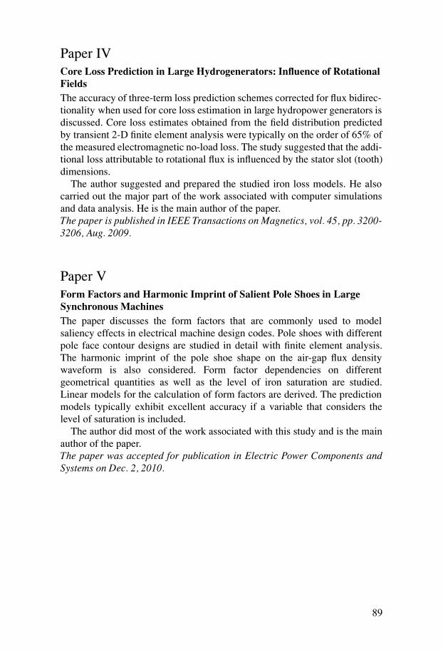
Paper IVCore Loss Prediction in Large Hydrogenerators: Influence of RotationalFieldsThe accuracy of three-term loss prediction schemes corrected for flux bidirec-tionality when used for core loss estimation in large hydropower generators isdiscussed. Core loss estimates obtained from the field distribution predictedby transient 2-D finite element analysis were typically on the order of 65% ofthe measured electromagnetic no-load loss. The study suggested that the addi-tional loss attributable to rotational flux is influenced by the stator slot (tooth)dimensions.

The author suggested and prepared the studied iron loss models. He alsocarried out the major part of the work associated with computer simulationsand data analysis. He is the main author of the paper.The paper is published in IEEE Transactions on Magnetics, vol. 45, pp. 3200-3206, Aug. 2009.

Paper VForm Factors and Harmonic Imprint of Salient Pole Shoes in LargeSynchronous MachinesThe paper discusses the form factors that are commonly used to modelsaliency effects in electrical machine design codes. Pole shoes with differentpole face contour designs are studied in detail with finite element analysis.The harmonic imprint of the pole shoe shape on the air-gap flux densitywaveform is also considered. Form factor dependencies on differentgeometrical quantities as well as the level of iron saturation are studied.Linear models for the calculation of form factors are derived. The predictionmodels typically exhibit excellent accuracy if a variable that considers thelevel of saturation is included.

The author did most of the work associated with this study and is the mainauthor of the paper.The paper was accepted for publication in Electric Power Components andSystems on Dec. 2, 2010.

89

Paper VIFinite Element Analysis of a Permanent Magnet Machine with TwoContra-rotating RotorsThe paper is concerned with basic no-load and load operational characteristicsof a PM generator with two contra-rotating rotors. Particular attention is de-voted to a pulsating inter-rotor flux distortion that is introduced via commoncore paths. It is shown that the distortion will be negligible if the stator coreis sufficiently wide. Load simulations of a slotless air-gap wound generatorappropriate for laboratory experiments indicated acceptable machine perfor-mance during identical speed rotor operation.

The author was responsible for computer simulations, data analysis, and isthe main author of the paper.The paper is published in Electric Power Components and Systems, vol. 37,pp. 1334-1347, Dec. 2009.

Paper VIIUse of a Finite Element Model for the Determination of Damping andSynchronizing Torques of Hydroelectric GeneratorsDamping and synchronizing torque coefficients are derived from time-steppedfinite element simulations of a hydroelectric generator connected to an infi-nite busbar. Torque coefficients are also derived from equivalent circuit sim-ulations, and a comparison between the results of the two methods is made.Particular attention is devoted to the impact of the damper winding type (conti-nuous or non-continuous) on the transient electromechanical response. Finiteelement models are found to exhibit both higher damping and higher syn-chronizing properties compared to equivalent circuit models of the studiedmachine type.

The author assisted in the development of the finite element model code,wrote the equivalent circuit simulation program and the parameter calculationscript, and carried out data analysis. He is the main author of the paper.The paper was submitted to The International Journal of Electrical Power andEnergy Systems for peer-review on May 11 2010.

90

Paper VIIIExperimental Study of the Effect of Damper Windings on SynchronousGenerator HuntingThe damping properties of a 75 kVA vertical-axis laboratory synchronous gen-erator with respect to electromechanical oscillations are determined experi-mentally. Damping time constants are derived from the oscillatory responsein electrical generator power initiated by step changes in the drive torque.The experimental responses are further compared with calculated responses,and the predictive precision of the used system model is assessed. The damp-ing in the tested unit is found to be highly susceptible to the impedance of theelectrical connection between the damper cages on adjacent poles. In two-axiscircuit terminology, this corresponds to the presence or absence of an effectiveq-axis damper.

The author installed the synchronization unit needed to achievegrid-connected generator operation, as well as voltage and current meteringdevices. He also assisted in the construction of the damper cage andperformed the experimental work and data analysis. He is the main author ofthe paper.The paper was submitted to Electric Power Components and Systems for peer-review on Feb. 3 2011.

Paper IXComparison of field and circuit generator models in single machineinfinite bus system simulationsThe paper compares the transient electromechanical response of a coupledfield-circuit model of a single machine infinite bus system to that of a modelwhere the generator is represented by equivalent circuits. The characteristicsof the two models are made equal as far as possible by using the finite elementmodel for the estimation of circuit parameters. The finite element model isfound to exhibit higher stiffness and higher damping. The differences in modelresponse are believed to be attributable to the diverse representations of therotor circuits.

The author wrote parts of the equivalent circuit simulation program andcontributed with ideas in the development process of the coupled field-circuitmodel. He also wrote a short section of the paper.The paper was presented at the XIX Int. Conf. on Electrical Machines, Rome,Italy, Sept. 6-8 2010.

91

Paper XDesign and construction of a synchronous generator test setupThe paper describes practical design considerations for a synchronous genera-tor test setup, to be used in studies of off-centered rotor operation. Advantagesand disadvantages of mechanical and instrumentation solutions are discussed.The slot harmonic amplitudes in the open-circuit armature voltage waveformfor two different damper winding configurations are provided as a first exam-ple of measurements.

The author contributed to the design, construction and installation of themagnetization equipment, the generator terminal enclosure and various mea-surement transducers. He performed the open-circuit voltage waveform anal-ysis and wrote a short section of the paper.The paper was presented at the XIX Int. Conf. on Electrical Machines, Rome,Italy, Sept. 6-8 2010.

92

11. Summary in Swedish

Elektromagnetisk analys av vattenkraftgeneratorerVattenkraften bibehåller sin position som världens viktigaste förnybaraenergislag. Tekniken är efter mer än hundra års utveckling både mogenoch tillförlitlig och verkningsgraden i storskaliga vattenkraftverk är myckethög. Medan vattenkraftsutbyggnaden ännu fortgår i Asien och Sydamerika,så genomgår de flesta europeiska länder med vattenkraftsresurseren fas av omfattande uppgradering och förnyelse av den befintligamaskinparken. I Sverige står vattenkraftindustrin inför utmaningar i formav kompetensöverföring till kommande generationer samt anpassning av deuppgraderade stationerna till förändrade driftförhållanden.

Datoriserade hjälpmedel har i grunden förändrat det ingenjörsmässigadesign- och analysarbete som är förknippat med konstruktionen av ettvattenkraftverk och dess huvudkomponenter. Den här doktorsavhandlingenbehandlar en av vattenkraftverkets nyckelkomponenter - generatorn -samt hur en rad designaspekter av elektromagnetisk natur kan hanterasmed moderna beräkningsmetoder. I synnerhet så demonstreras en radtillämpningar av finita elementmodeller samt roterande fältmodeller.

I en första studie presenteras en roterande fältmodell för noggrann beräkn-ing av den magnetiska luftgapsflödestäthetens vågform. En förenklad metodför att beräkna dämplindningens magnetiska reaktionsflöde förevisas också.Modellen har med framgång använts för att beräkna spårtoner i en genera-tors tomgångsspänningskurvform, samt strömmar i dämplindningen vid såvältomgång som vid last.

En annan studie har tillägnats de magnetiska rotationsförluster som upp-kommer till följd av bidirektionella magnetflöden i statorkärnan. I kombina-tion med vissa dynamiska effekter befanns rotationsförlusterna typiskt ökaden totala järnförlustskattningen med ca 28%. Beräkningsresultaten påvisadeäven en korrelation mellan rotationsförlusternas storlek och statorspårens di-mensioner.

Avhandlingen presenterar även linjära modeller för beräkning av formfak-torer för utpräglade polskor av godtycklig geometri och mättnadsgrad. Enöversikt av hur polplattan bör väljas att få önskad luftgapsflödestäthetsvåg-form ges.

Slutligen redovisas en numerisk studie av de elektromekaniskaegenskaperna hos finita elementmodeller av nätanslutna vattenkraftgenerator.Kortslutningsringens betydelse för modellens dämpande egenskaper vid

93

rotorvinkelpendlingar betonas särskilt. Slutsatserna från denna studieverifierades i en serie experiment, där rotorvinkelpendlingar initierades medkontrollerade momentstötar.

94

Acknowledgments

The research presented in this thesis was carried out as a part of TheSwedish Hydropower Centre (Svenskt Vattenkraftcentrum, SVC). SVC wasestablished by The Swedish Energy Agency, Elforsk, The Swedish NationalGrid Agency together with Luleå University of Technology, The RoyalInstitute of Technology, Chalmers University of Technology and UppsalaUniversity.

All members of the SVC steering committee for research in the field ofturbines and generators are acknowledged for guidance and advice.

Anders Hagnestål, Simon Tyrberg and Katarina Yuen-Lasson, UppsalaUniversity, are acknowledged for their help with proof-reading.

The author additionally would like to express gratitude to these persons:

Niklas Dahlbäck, Vattenfall Vattenkraft, Göran Franzén, BEVI AB, ThomasGötschl, Uppsala University, Gunnel Ivarsson, Uppsala University,Dr. Thommy Karlsson, Vattenfall Power Consultant, Peter Ljung, VattenfallVattenkraft, Gunilla Ries-Jende, Vattenfall Power Consultant, Ulf Ring,Uppsala University, Richard Perers, VG Power / Voith Siemens, Dr. AnnaWolfbrandt, E-ON ES, and Dr. Arne Wolfbrandt, Uppsala University.

Finally, a special thanks is addressed to the following persons:

My colleague Johan Bladh, Vattenfall Research and Development, forhis friendship, good advice and support during these four years of joint efforts.

My colleague Mattias Wallin, Uppsala University, for rewarding discussions.The author is also indebted to Mr. Wallin for his untiring efforts with the testgenerator.

My supervisor Dr. Urban Lundin, Uppsala University, for his guidance andsupport throughout the project.

95

My assistant supervisor Prof. Mats Leijon, Uppsala University, forinspiration and support.

96

References

[1] ET 2009:29. Energy in Sweden - Facts and Figures. Technical report, TheSwedish Energy Agency, 2009.

[2] G. Traxler-Samek, A. Schwery, and E. Schmidt. Analytic calculation of thevoltage shape of salient pole synchronous generators including damper windingand saturation effects. COMPEL, 22:1126–1141, 2003.

[3] O. Bottauscio, A. Canova, M. Chiampi, and M. Repetto. Iron losses in electricalmachines: Influence of different material models. IEEE Trans. Magn., 38:805–808, 2002.

[4] D.M. Ionel, M. Popescu, M. McGilp, T.J.E. Miller, S. Dellinger, and R.J. Hei-deman. Computation of Core Losses in Electrical Machines Using ImprovedModels for Laminated Steel. IEEE Trans. Magn., 43:1554–1564, 2007.

[5] L. Ma, M. Sanada, S. Morimoto, and Y. Takeda. Prediction of Iron Loss in Ro-tating Machines With Rotational Loss Included. IEEE Trans. Magn., 39:2036–2041, 2003.

[6] N. Stranges and R.D. Findlay. Methods for Predicting Rotational Iron Losses inThree Phase Induction Motor Stators. IEEE Trans. Magn., 36:3112–3114, 2000.

[7] J.G. Zhu and V.S. Ramsden. Improved formulations for Rotational Core Lossesin Rotating Electrical Machines. IEEE Trans. Magn., 34:2234–2242, 1998.

[8] R.D. Findlay, N. Stranges, and D.K. MacKay. Losses due to Rotational Flux inThree-Phase Induction Motors. IEEE Trans. Energy Convers., 9:543–549, 1994.

[9] A.R. Hagen, A. Binder, M. Aoulkadi, T. Knopik, and K. Bradley. Comparison ofmeasured and analytically calculated stray load losses in standard cage inductionmachines. In Proc. of the XVIII Int. Conf. on Electrical Machines (ICEM 2008),Vilamoura, Portugal, 2008.

[10] G. Díaz, C. González-Morán, P. Arboleya, and J. Gómez-Aleixandre. Analyt-ical Interpretation and Quantification of Rotational Losses in Stator Cores ofInduction Motors. IEEE Trans. Magn., 43:3861–3867, 2007.

[11] G. Traxler-Samek, A. Schwery, R. Zickermann, and C. Ramirez. Optimized Cal-culation of Losses in Large Hydropower Generators Using Statistical Methods.In Proc. of the XVI Int. Conf. on Electrical Machines (ICEM 2004), Cracow,Poland, 2004.

97

[12] A. Nakahara, K. Takahashi, K. Ide, J. Kaneda, K. Hattori, T. Watanabe, H. Mogi,C. Kaido, E. Minematsu, and K. Hanzawa. Core loss in turbine generators:Analysis of no-load core loss by 3D magnetic field calculation. In Proc. of theXVI Int. Conf. on Electrical Machines (ICEM 2004), Cracow, Poland, 2004.

[13] B. Hague. The shape of pole-shoe required to produce a sinusoidal distributionof air-gap flux density. Journal of the I.E.E., 62:921–929, 1924.

[14] R.H. Wieseman. Graphical Determination of Magnetic Fields. Practical Appli-cations to Salient-Pole Synchronous Machine Design. AIEE Trans., 46:141–154, 1927.

[15] T.A. Lipo. Introduction to AC Machine Design, chapter 8, pages 460–466. Wis-consin Power Electronics Research Center, University of Wisconsin, 2004.

[16] T. K. Nielsen, J. Røyrvik, J. Ramdal, and O. G. Dahlhaug. Propeller turbinewith two contra-rotating impellers and built-in generators. In Proc. of the 23rdInt. Association of Hydraulic Eng. and Research Symposium, Yokohama, Japan,Oct. 2006.

[17] J.A. Clarke, G. Connor, A.D. Grant, C.M. Johnstone, and D. Mackenzie. Devel-opment of a contra-rotating tidal current turbine and analysis of performance. InConf. proceedings EWTEC 2007 - 7th European Wave and Tidal Energy Con-ference, Porto, Portugal, Sept. 2007.

[18] F. Caricchi, F. Crescimbini, and E. Santini. Basic principle and design criteria ofaxial-flux PM machines having counterrotating rotors. IEEE Trans. Ind. Appl.,pages 1062–1068, 1995.

[19] R.E. Doherty and C.A. Nickle. Synchronous machines - III. AIEE Trans., 46:1–18, 1927.

[20] R.H. Park. Two-Reaction Theory of Synchronous Machines - II. AIEE Trans.,52:352–354, 1933.

[21] C. Concordia. Synchronous Machine Damping and Synchronizing Torques.AIEE Trans., 70:731–737, 1951.

[22] R.V. Shepherd. Synhronizing and Damping Torque Coefficients of SynchronousMachines. AIEE Trans., 80:180–189, 1961.

[23] A.A. Shaltout and M.A. Abdel-Halim. Damping and Synchronizing Torquesof Salient-Pole Generators with Accurate Representation of Saturation. IEEETrans. Energy Convers., 10:1–9, 1995.

[24] I. Boldea. Synchronous Generators, chapter 7, pages 4–42 – 4–43. CRC PressTaylor & Francis, 2006.

[25] A. Blondel. The Two-Reaction Method for Study of Oscillatory Phenomenain Coupled Alternators. Revue générale de l’électricité, 13:235–251, 515–531,February and March 1923.

98

[26] R.H. Park. Two-Reaction Theory of Synchronous Machines - GeneralizedMethod of Analysis, Part I. AIEE Trans., 48:716–727, 1929.

[27] A.I. Megahed and O.P. Malik. Simulation of Internal Faults in SynchronousGenerators. IEEE Trans. Energy Convers., 14:1306–1311, 1999.

[28] X. Wang, S. Shen, W. Wang, Y. Sun, and L. Xu. A study of Armature WindingInternal Faults for Turbogenerators. IEEE Trans. Ind. Appl., 38:625–631, 2002.

[29] IEEE Power Engineering Society. IEEE Std. 1110 Guide for Synchronous Gen-erator Modeling Practices and Applications in Power System Stability Analyses,2002.

[30] V. Atarod, P.L. Dandeno, and M.R. Iravani. Impact of Synchronous MachineConstants and Models on the Analysis of Torsional Dynamics. IEEE Trans.Power Syst., 7:1456–1463, 1992.

[31] M.A. Abdel-Halim and C.D. Manning. Modelling saturation of laminatedsalient-pole synchronous machines. IEE Proceedings pt. B, 134:215–223, 1987.

[32] M. Ladjavardi, M.A.S. Masoum, and S.M. Islam. Impact of SG Damper Wind-ings on Small-Signal Stability of a Distorted SMIB Including Time and SpaceHarmonics. In Proc. of the 40th North American Power Symposium, Calgary,Canada, 2008.

[33] P. Kundur. Power System Stability and Control, chapter 4, pages 139–159.McGraw-Hill, 1994.

[34] R. Wamkeue, I. Kamwa, F. Baetscher, and J. El Hayek. A New and EfficientApproach for Analysis of a Saturated Synchronous Generator Under the LoadRejection Test. Electric Power Components and Systems, 34:539–563, 2006.

[35] J. Lidenholm and U. Lundin. Estimation of Hydropower Generators ParametersThrough Field Simulations of Standard Tests. IEEE Trans. Energy Convers.,25:931–939, 2010.

[36] S. Lagerkvist. Kompendium i konstruktiv elektromaskinkära Del II - Synkron-maskinen, Appendix. Göteborg, 1963, in Swedish.

[37] N. Bianchi. Electrical Machine Analysis using Finite Elements, chapter 2, pages25–26. Taylor & Francis, Boca Raton, FL, 2005.

[38] P.J. Turner and D.C. MacDonald. Finite Element Prediction of Steady StateOperation of a Turbine-Generator Using Conductivity Matrices. IEEE Trans.Magn., 17:3262–3264, 1981.

[39] J.L. Coulomb. A methodology for the determination of global electromechanicalquantities from a finite element analysis and its application to the evaluation ofmagnetic forces, torques and stiffness. IEEE Trans. Magn., 19:2514– 2519,1983.

99

[40] M. Ranlöf. Core Loss Prediction in Hydroelectric Generators and Analysis of aContra-Rotating Machine Topology. Licentiate Thesis, 2009.

[41] A.B.J Reece and T.W. Preston. Finite Element Methods in Electrical PowerEngineering, chapter 3, pages 34–35. Oxford University Press, Oxford, UK,2000.

[42] I.A. Tsukerman, A. Konrad, G. Meunier, and J.C. Sabonnadière. Coupled field-circuit problems: Trends and accomplishments. IEEE Trans. Magn., 29:1701–04, 1993.

[43] D. Shen and G. Meunier. Modeling of Squirrel Cage Induction Machines by theFinite Elements Method Combined with the Circuit Equations. In Proc. of theInt. Conf. on Evolution and Aspects of Induction Machines, Turin, Italy, 1986.

[44] C.N. Ashtiani and D.A. Lowther. The Use of Finite Elements in the Simula-tion of the Steady State Operation of a Synchronous Generator with a KnownTerminal Loading. IEEE Trans. Magn., 19:2381–2384, 1983.

[45] A.M. Knight, H. Karmaker, and K. Weber. Use of a permeance model to pre-dict force harmonic components and damper winding effects in salient-pole syn-chronous machines. IEEE Trans. Energy Convers., 17:478–484, 2002.

[46] G. Traxler-Samek, T.Lugand, and A. Schwery. Additional Losses in the DamperWinding of Large Hydrogenerators at Open-Circuit and Load Conditions. IEEETrans. Ind. Electronics, 57:154–160, 2010.

[47] J.H. Walker. Slot ripples in alternator E.M.F. waves. Journal I.E.E., 96 PartII:81–92, 1949.

[48] E.J.J. Rocha, M.K. Uemori, and A. De Arruda Penteado Junior. The damperwinding influence upon salient pole synchronous generator electromotive force.In 1997 IEEE Int. Electric Machines and Drives Conference Record, Milwau-kee, WI, USA, May 1997.

[49] S. Keller, M.T. Xuan, and J-J. Simond. Computation of the No-Load VoltageWaveform of Laminated Salient-Pole Synchronous Generators. IEEE Trans.Ind. Appl., 42:681–687, 2006.

[50] P.A. Hargreaves, B.C. Mecrow, and R. Hall. Open Circuit Voltage Distortionin Salient Pole Synchronous Generators with Damper Windings. In Proc. ofthe 5th Int. Conf. on Power Electronics, Machines and Drives (PEMD 2010),Brighton, UK, 2010.

[51] E.I. Pollard. Calculation of No-Load Damper Winding Loss. AIEE Trans.,51:477–483, 1932.

[52] J. Matsuki, T. Katagi, and T. Okada. Slot Ripples in the Damper Windings of aSalient-Pole Synchronous Generator. IEEE Trans. Energy. Convers., 9:126–134,1994.

100

[53] A.M. Knight, S. Troitskaia, N. Stranges, and A. Merkhouf. Analysis of largesynchronous machines with axial skew, part 2: inter-bar resistance, skew andlosses. IET Electric Power Appl., 3:398–406, 2009.

[54] D.G. Dorell and A.C. Smith. Calculation of U.M.P in Induction Motors withSeries or Parallel Winding Connections. IEEE Trans. Energy Convers., 9:304–310, 1994.

[55] W. Oliveira, M. Uemori, J. Rocha, and R. Carlson. Reduction of unbalancedmagnetic pull (UMP) due to equipotential connections among parallel circuitsof the stator winding. In Proc. of the Int. Electric Machines and Drives Conf.(IEMDC), pages 771–777, May 2009.

[56] T.A. Lipo. Introduction to AC Machine Design, chapter 2, pages 64–82. Wis-consin Power Electronics Research Center, University of Wisconsin, 2004.

[57] H. Annell. The alternating current impedance of a solid conductor of circularcross section placed in a semi-closed circular slot. Trans. of the Royal Instituteof Technology Stockholm, 200:1–34, 1963.

[58] R.L. Stoll. The analysis of eddy currents, chapter 2, pages 23–26. ClarendonPress, 1974.

[59] J.H. Walker. Parasitic losses in synchronous-machine damper windings. JournalI.E.E., 94 Part II:13–25, 1947.

[60] F. Fiorillo and A. Novikov. An Improved Approach to Power Losses in MagneticLaminations under Nonsinusoidal Induction Waveform. IEEE Trans. Magn.,26:2904–2910, 1990.

[61] A.J. Moses. Importance of rotational losses in rotating machines and transform-ers. J. Materials Eng. and Performance, 1:235–244, 1992.

[62] G. Bertotti. General Properties of Power Losses in Soft Ferromagnetic Materi-als. IEEE Trans. Magn., 24:621–629, 1988.

[63] J.D. Lavers, P.P. Biringer, and H. Hollitscher. A Simple Method of Estimat-ing the Minor Loop Hysteresis Loss in Thin Laminations. IEEE Trans. Magn.,14:386–388, 1978.

[64] G. Bertotti, A. Canova, M. Chiampi, D. Chiarabaglio, F. Fiorillo, and A.M. Ri-etto. Core loss prediction combining physical models with numerical field anal-ysis. J. Magn. and Magn. Mat., 133:647–650, 1994.

[65] J. Clarke, G. Connor, A. Grant, C. Johnstone, and S. Ordonez-Sanchez. Contra-rotating Marine Current Turbines: Single Point Tethered Floating System - Sta-bility and Performance. In Proc. of the VIII European Wave and Tidal EnergyConf. (EWTEC 2009), Uppsala, Sweden, 2009.

[66] Y. Yeh, D.G. Dorrell, and M. Hsieh. Different Arrangements for Dual-Rotor Dual-Output Radial-Flux Motors. In Proc. of IEEE Energy ConversionCongress and Exposition (ECCE), Atlanta, GA, Sept. 2010.

101

[67] J.B. Danilevich, V.N. Antipov, I. Yu. Krushinina, Y.Ph. Khozikov, A.A. Pono-mareva, and L.Yu. Shtainle. Peculiar design of permanent magnet synchronousmotor. In Proc. XIX Int. Conf. on Electrical Machines, Rome, Italy, Sept. 2010.

[68] F.R. Schleif, G.E. Martin, and R.R. Angell. Damping of System Oscillationswith a Hydrogenerating Unit. IEEE Trans. Power App. Syst., 86:438–442, 1967.

[69] F.P. deMello and C. Concordia. Concepts of Synchronous Machine Stabilityas Affected by Excitation Control. IEEE Trans. Power App. Syst., 88:316–329,1969.

[70] R.T.H. Alden and A.A. Shaltout. Analysis of Damping and SynchronizingTorques, Part I - a General Calculation Method. IEEE Trans. Power App. Syst.,98:1696–1700, 1979.

[71] R. Escalera-Perez, M.A. Arjona-Lopez, E. Melgoza-Vasquez, E. Campero-Littlewood, and C. Aviles-Cruz. A comprehensive finite-element model of aturbine-generator infinite-busbar system. Finite Elements in Analysis and De-sign, 40:485–509, 2004.

[72] P. Kundur. Power System Stability and Control, chapter 15, pages 1026–1033.McGraw-Hill, 1994.

[73] P. Kundur. Power System Stability and Control, chapter 3, pages 128–135.McGraw-Hill, 1994.

[74] P. Kundur. Power System Stability and Control, chapter 3, pages 850–853.McGraw-Hill, 1994.

[75] C. Concordia. Steady-State Stability Analysis of Synchronous Machines as Af-fected by Voltage Regulator Characteristics. AIEE Trans., 63:215–220, 1944.

[76] R.E. Doherty and C.A. Nickle. Synchronous Machines - I, An Extension ofBlondel’s Two-Reaction Theory. AIEE Trans., 45:912–926, 1926.

[77] IEEE Power Engineering Society. IEEE Std. 421.5 Recommended Practice forExcitation System Models for Power System Stability Studies, 2005.

[78] G. Kron. Equivalent Circuits for the Hunting of Electric Machinery. AIEETrans., 61:290–296, 1942.

[79] M.M. Liwschitz-Garik. Starting Performance of Salient-Pole Synchronous Mo-tors. AIEE Trans., 59:913–919, 1940.

102