electrohydrodynamic stability

Electrohydrodynamic Stability

Chuan-Hua Chen∗

Department of Mechanical Engineering and Materials Science,Duke University, Durham, NC, USA

Abstract Stability of electrohydrodynamic flows is essential to avariety of applications ranging from electrokinetic assays to electro-spray ionization. In this series of lecture notes, a few basic conceptsof electrohydrodynamic stability are illustrated using two modelproblems, electrokinetic mixing flow and electrohydrodynamic cone-jet, respectively wall-bounded and free surface flow. After a reviewof the governing equations, spatiotemporal analysis of the two exam-ple problems is presented using linearized bulk- or surface-coupledmodels. The operating regimes for these flows are discussed withinthe framework of electrohydrodynamic stability.

1 Introduction

Electrohydrodynamic transport phenomena are fundamental to a varietyof engineering applications such as electrokinetic assays, electrospray ion-ization, electro-coalescence and mixing, electrostatic printing and spinning.Although unstable flow is desired in certain applications (e.g. in mixing),a stable flow is typically the preferred state (e.g. in assays and ionization).In either case, the demarcation between the stable and unstable states is ofpractical importance. The theme of these lecture notes is to develop a sys-tematic methodology in identifying such stability boundaries of electrohy-drodynamic flows. The topics have been selected mainly for their pedagog-ical value in illustrating the basic concepts in continuum electromechanicsand hydrodynamic stability, often motivated by practical applications andbacked by experimental observations. Although the governing equationsand analysis methodology should be of general applicability, no attempt

∗I am indebted to the organizer, Dr. A. Ramos, who graciously helped on delivering the

videotaped lectures as a result of visa complications that prevented me from traveling

to CISM. My Ph.D. adviser J. G. Santiago helped on the initial outline of the lecture

notes. Drs. M. P. Brenner and A. M. Ganan-Calvo provided helpful correspondence

about their research. This work was funded in part by an NSF CAREER Award.

A. Ramos (ed.), Electrokinetics and Electrohydrodynamics in Microsystems

© CISM, Udine 2011

C.H. Chen, "Electrohydrodynamic stability," in Electrokinetics and Electrohydrodynamics in Microsystems (Ed. A. Ramos), Springer, pp. 177-220 (2011).

178 Chuan-Hua Chen

has been made to comprehensively review the rapidly expanding field ofelectrohydrodynamic stability. Extensive coverage of electrohydrodynamicsand the associated flow stability can be found in Melcher and Taylor (1969);Melcher (1981); Saville (1997); Fernandez de la Mora (2007); Chang and Yeo(2010). In addition, an educational film developed by Melcher (1974) offersmany intuitive insights on electrohydrodynamics.

2 Basics of Electrohydrodynamics

Electrohydrodynamics deals with the interaction of electric and flow fieldswhere the Ohmic model is frequently an excellent approximation (Melcherand Taylor, 1969; Saville, 1997). In this section, we first present an intuitivederivation of the Ohmic model and clearly identify the assumptions behind.We then offer some physical insights on the Maxwell stress tensor whichplays the crucial role of coupling the electrostatics and hydrodynamics. Fi-nally, we discuss the governing equations for both surface- and bulk-coupledmodels. The surface-coupled model takes essentially the same form as inMelcher and Taylor (1969) and Saville (1997), while the bulk-coupled modeltakes roots in Levich (1962) and Melcher (1981).

2.1 Ohmic model

Electrohydrodynamic systems can usually be approximated as electro-quasistatic (Saville, 1997). In the absence of external magnetic fields, mag-netic effects can be ignored completely. The electrostatic field is solenoidal,

∇×E = 0. (1)

The electric field (E) obeys the Gauss’s law, which for electrically linearmedium reduces to,

∇ · εE = ρf , (2)

where ε is the permittivity, and ρf is the free charge density. The free chargedensity is related to the current (i) by the charge conservation equation,

∂ρf∂t

+∇ · i = 0. (3)

In the Ohmic model, or the so-called leaky dielectric model (Saville,1997), an Ohmic constitutive law of the conduction current is assumed(Melcher and Taylor, 1969),

i = iC + iO = ρfv + σE, (4)

Electrohydrodynamic Stability 179

where iC = ρfv is the convection current, iO = σE is the Ohmic current, vis the fluid velocity, and σ is the electrical conductivity. The Ohmic modelcan be derived from the electro-diffusive transport of individual chargedions (Melcher, 1981; Saville, 1997; Levich, 1962). We assume for algebraicsimplicity a monovalent binary electrolyte which is fully dissociated withconstant properties (Chen et al., 2005). For derivations involving multiva-lent electrolyte and chemical reaction, see Levich (1962) and Saville (1997),respectively. In the Ohmic model, bulk quantities of conductivity and chargedensity are tracked instead of individual ions. The charge density (ρf ) andelectric conductivity (σ) are related to the ionic concentrations through

ρf = F (c+ − c−), (5)

σ = F 2(c+m+ + c−m−), (6)

where F is the Faraday constant, c± is the cationic/anionic molar concen-tration, and m± is the ionic mobility (in molN−1 ms−1).

The key simplifying assumption in the derivation is electro-neutrality,which can be assumed in the limit of (Chen et al., 2005)

Θ1 =Fm+ρf

σ=

c+ − c−c+ + m−

m+c− 1, (7)

where Θ1 represents the ratio of cationic and anionic concentration differ-ence (which contributes to the charge density) to the total concentrationof ions (which contributes to the electrical conductivity). Applying theGauss’s law,

Θ1 =Fm+ρf

σ∼ Fm+∇ · εE

σ∼ ε/σ

Lr/m+FE∼ τe

τr, (8)

where τe = ε/σ is the charge relaxation time, m+FE is by definition theelectro-migration velocity of the cation, Lr is a reference length scale overwhich the electric field varies (typically the smallest length scale of the elec-trohydrodynamic system), and τr is the time scale to travel Lr by electro-migration. Therefore, electro-neutrality is an excellent approximation formost electrolyte solutions (typically with σ > 10−4 S/m) with fast chargerelaxation (typically with τe < 10 μs), because the charge relaxation time ismuch shorter than the electrohydrodynamic time scale of interest (typicallywith τr > 1 ms). When the electrolyte solution is approximately neutral,

c+ � c− = c; | c+ − c− | c, (9)

180 Chuan-Hua Chen

where c is the reduced ionic concentration (Levich, 1962). Under electro-neutrality, the conductivity is proportional to this reduced concentrationby

σ = F 2(m+ +m−)c. (10)

To derive the governing equation for conductivity, we start from theNernst-Planck equations for ionic species (Levich, 1962),

∂c+∂t

+∇ · c+v = D+∇2c+ −m+F∇ · c+E, (11)

∂c−∂t

+∇ · c−v = D−∇2c− +m−F∇ · c−E, (12)

where D± is the ionic diffusivity. The diffusivity and mobility is related byEinstein’s relation D± = RTm± where R is the universal gas constant andT is the absolute temperature. Subtracting Eqs. 11 and 12 and noting theelectro-neutrality condition,

(D+ +D−)F∇ · cE � RT (D+ −D−)∇2c, (13)

where the equality holds to the leading order of ionic concentrations. Sub-stituting Eq. 13 to Eq. 11 and noting Eq. 10, the electro-diffusion equationbecomes

∂σ

∂t+∇ · σv = Deff∇2σ, (14)

where Deff is an effective diffusivity,

Deff =2D+D−D+ +D−

. (15)

To derive the equation for charge density, we subtract Eqs. 11 and 12again in an exact manner,

∂(c+ − c−)∂t

+∇·(c+−c−)v = ∇2(D+c+−D−c−)−F∇·(m+c++m−c−)E,

(16)or in terms of bulk quantities,

∂ρf∂t

+∇ · (ρfv + iD + σE) = 0, (17)

where the diffusive current iD = −F∇(D+c+−D−c−) � −(D+−D−)F∇c(Levich, 1962). Eq. 17 reduces to the the charge conservation equation inthe Ohmic regime,

∂ρf∂t

+∇ · ρfv = −∇ · σE, (18)


when the diffusive current can be neglected, i.e.

Θ2 =

∣∣∣∣ iDiO∣∣∣∣ 1. (19)

In electrohydrodynamic systems, the diffusive current is usually much smallerthan the Ohmic conduction current. The ratio of the two currents scales as,

Θ2 =

∣∣∣∣ iDiO∣∣∣∣ ∼ (D+ −D−)F∇c

(m+ +m−)F 2cE∼ D+ −D−

D+ +D−RT

F

∇c

Ec∼ RT/F

ELr∼ ΦT

Φr,

(20)where ΦT = RT/F (25 mV at room temperature) is the thermal voltagedriving the diffusive current, and Φr is the reference voltage drop along aconcentration gradient. Since the applied electric field is typically high in anelectrohydrodynamic system, the diffusive current can be safely neglected(i.e. Eq. 19 is valid) for most practical cases. For example, with a field of105 V/m, Θ2 1 for a diffusive interface as thin as 1 μm.

The Ohmic model consists of the conservation equations for conductiv-ity (Eq. 14) and charge density (Eq. 18). Physically, the material derivativeof conductivity and charge density is balanced by the divergence of an ef-fective diffusive flux and Ohmic current flux, respectively. The underlyingassumptions in the Ohmic model are instantaneous charge relaxation (Eq. 7)and negligible diffusive current (Eq. 19).1 Both assumptions hold for mostpractical electrohydrodynamic systems driven by direct-current (DC) fields,where the time scale of interest is typically above 1 ms and the length scaleof interest is typically above 1 μm. With rapid charge relaxation, the elec-trolyte solution is approximately electro-neutral in the bulk and the cationsand anions are almost always paired together, as the difference in cationicand ionic concentrations is very small compared to the background con-centration of electrolytes. Consequently, conductivity becomes a conservedmaterial property with an effective diffusivity averaging the cationic andanionic properties. Note that the Ohmic model does not work inside elec-tric double layer, where the net charged layer has a typical thickness of wellbelow 1 μm.

2.2 Maxwell stress

The electrostatics and hydrodynamics are coupled together through theMaxwell stress tensor. In vacuum, the Coulombic force density exerted on

1Although we have assumed constant properties (D± and m±) in the derivation, the

Ohmic model consisting of Eqs. 14 and 18 are generally believed to hold for cases with

non-constant properties, e.g. due to temperature gradients.

182 Chuan-Hua Chen

free charges can be rearranged noting the solenoidal nature of the electro-static field (Panofsky and Phillips, 1962),

fe0 = ρfE = (∇ · ε0E)E

= ∇ ·(ε0EE− 1

2ε0E

2I

)= ∇ ·Te

0, (21)

where ε0 is the permittivity of vacuum, I is the identity matrix, and Te0 is

the Maxwell stress (or electric stress) tensor in vacuum.The derivation of Maxwell stress tensor for a dielectric medium is rather

complicated (Melcher, 1981; Panofsky and Phillips, 1962). Here, we sum-marize salient points of the Maxwell stress tensor and refer the readers toMelcher (1981) for details. The electrical force density can be derived us-ing either the Kelvin approach or the Korteweg-Helmholtz approach. TheKelvin force density is useful for appreciating the underlying microscopicelectromechanics, while the Korteweg-Helmholtz force density is more use-ful for predicting the consequences of electromechanical coupling (Melcher,1974). The Kelvin force density is the sum of the Coulombic force exertedon free charges and the polarization force exerted on the dipoles (Melcher,1981),

feK = ρfE+P · ∇E = (∇ · εE)E+ (ε− ε0)E · ∇E

= ∇ ·(εEE− 1

2ε0E

2I

)= ∇ ·Te

K , (22)

where P is the polarization density, and TeK is the Maxwell stress tensor

corresponding to the Kelvin force density. The key concept due to Kelvin isthat the polarization force is exerted on the dipoles (P), not on individualpolarization charges (−∇ ·P) (Melcher, 1981). The Korteweg-Helmholtzforce density stems from thermodynamic principles. For an electrically lin-ear medium with polarization dependent on mass density (ρ) and tempera-ture (T ) alone, the force density can be shown to be,

feKH = ρfE− 1

2E2∇ε+∇

[1

2ρ

(∂ε

∂ρ

)T

E2

]

= ∇ ·[εEE− 1

2εE2I+

1

2ρ

(∂ε

∂ρ

)T

E2I

]= ∇ ·Te

KH , (23)

where the last term is the electrostriction force density associated with vol-umetric change in the material; See Melcher (1981, Sec. 3.7) for a detailedderivation. The Kelvin and Korteweg-Helmholtz force densities are different


by the gradient of a scalar,

feK − feKH = ∇[1

2(ε− ε0)E

2 − 1

2ρ

(∂ε

∂ρ

)T

E2

], (24)

which can be absorbed into a lumped pressure. The difference representsthe interaction between dipoles, which is omitted in the Kelvin derivation.For incompressible flow, where pressure becomes a “left-over” variable, anytwo force densities differing by the gradient of a scalar pressure will give riseto the same incompressible deformation (Melcher, 1981). Both force den-sities, if used consistently, will yield the same answer as far as incompress-ible mechanical deformation is concerned. Because the actual electric forcedistributions of the two approaches are ususally very different, we stressthat the same force density should be used consistently; See an example inMelcher (1981, Sec. 8.3).

Hereon, we shall restrict our discussions to the practically importantcase of electrically linear, incompressible dielectric medium, and consistentlyadopt the Korteweg-Helmholtz force density,

fe = ρfE− 1

2E2∇ε

= ∇ ·(εEE− 1

2εE2I

)= ∇ ·Te. (25)

When the permittivity is that of vacuum, the Maxwell stress tensor Te inEq. 25 reduces to Te

0 in Eq. 21. This similarity enables us to take advantageof the “bisect rule” graphically shown in Figure 1 (Panofsky and Phillips,1962, Sec. 6-5). The bisect rule is useful in graphically identifying thedirection of electric stress when the field direction is known. A few exampleapplications of the bisect rule are shown in Figure 2.

From the Korteweg-Helmholtz force density in Eq. 25 and the corre-sponding bisect rule in Figure 2, it is apparent why a leaky dielectric isnecessary to support any tangential electric stress at electrostatic interfaces(Melcher and Taylor, 1969). For a perfect conductor such as the chargeddrop in (a), the Coulombic force is always along the electric field which isperpendicular to the interface. For a perfect dielectric such as a dielectricjet in (b), the polarization force is always along the permittivity gradientwhich is again perpendicular to the interface. For a leaky dielectric withfinite, non-zero conductivity and permittivity, a tangential shear stress candevelop such as in the electrified cone in (c), where the electric field at 45◦

to the surface normal gives rise to a shear force along the conical surface.

184 Chuan-Hua Chen

E

Fe

n

Figure 1. The bisect rule: the electric field (E) bisects the angel betweenthe normal to the surface (n) and the direction of the resultant force (Fe)acting on the surface (dS). In a dielectric medium with a local permittivityof ε, the magnitude of the electric force is F e = T edS = 1

2εE2dS. After

Panofsky and Phillips (1962).

+++

+

++

+

+

EFe n

(a) (b) (c)

Figure 2. Example applications of the bisect rule: (a) on a charged con-ducting drop, the surface normal is along the direction of the electric field,hence the Coulombic repulsion is also along the direction of the electricfield; (b) on a dielectric liquid jet, the surface normal is perpendicular tothe electric field, hence the polarization force is perpendicular to the elec-tric field and pointing outward; (c) on a leaky dielectric cone, the surfacenormal is at 45◦ to the electric field, hence the (total) electric force is alongthe tangential direction of the cone which is also at 45◦ to the electric field.


2.3 Governing equations

To summarize, the electrohydrodynamic leaky dielectric model consistsof the following equations:

∇×E = 0, (26a)

∇ · εE = ρf , (26b)

∂ρf∂t

+∇ · ρfv = −∇ · σE. (26c)

∇ · v = 0, (26d)

ρ∂v

∂t+ ρv · ∇v = −∇p+ μ∇2v + ρfE− 1

2E2∇ε, (26e)

where p is the pressure and μ is the dynamic viscosity. The electric bodyforces in the momentum equation (Eq. 26e) include both a Coulombic anda polarization component. These equations are valid for incompressible,electrically linear leaky dielectrics with rapid charge relaxation and negligi-ble diffusive current, for example, aqueous electrolyte solutions. The set ofgoverning equations (26) is closed if the distribution of material properties(ε, σ, μ) is either given or modeled with additional equations.

We have employed the electro-neutrality assumption in the derivation ofthe Ohmic model, but kept the charge density in the governing equations.Although the material derivative of ρf may often be neglected in the chargeconservation equation (Eq. 26c), it will not be appropriate to neglect theCoulombic body force term ρfE in the momentum equation (Eq. 26e) be-cause this force drives the electrohydrodynamic flow. Combining the chargeconservation equation (Eq. 26c) and the Gauss’s law (Eq. 26b) (Melcher,1974),

DρfDt

=ρfτe− σE ·

(∇σ

σ− ∇ε

ε

). (27)

In regions of uniform conductivity and permittivity, the net free chargedecays with the charge relaxation time for an observer following a particleof fixed identity (Melcher and Taylor, 1969):

ρf = ρf,0e−t/τe . (28)

Therefore, unless an element of material having uniform properties can betraced along a particle line to a source of net charge, it supports no netcharge (Melcher and Taylor, 1969). In inhomogeneous material, however,free charge density can be generated by an electric field component alongthe gradients of conductivity and/or permittivity.

186 Chuan-Hua Chen

Systems having nonuniform properties can be modeled either as a bulkregion with continuously varying properties or as adjoining regions withpiecewise uniform properties (Melcher, 1981; Hoburg and Melcher, 1976).Since interesting electrohydrodynamics often happen at material interfaces,we shall discuss two approaches to close the problem depending on theinterfacial sharpness (Hoburg and Melcher, 1976).

In the bulk-coupled model for a diffusive interface, additional equationsof the materials properties must be added. For example, in aqueous elec-trolytes the permittivity is essentially constant but the conductivity varia-tion can be significant; in this case, the “conservation” equation of conduc-tivity from the Ohmic model can be used,

∂σ

∂t+∇ · σv = Deff∇2σ. (29)

In the surface-coupled model for a sharp interface, the material proper-ties are usually piecewise constant on either side of the interface; However,jump conditions are needed to relate the interfacial and bulk properties.Except for the empirical no-slip condition (Eq. 30e), the following jumpconditions can be obtained by integrating the differential equations acrossthe interface (Melcher and Taylor, 1969; Melcher, 1981; Saville, 1997; Leal,2007),

n× ‖E‖ = 0, (30a)

n · ‖εE‖ = qs, (30b)

∂qs∂t

+∇s · (qsv) = −n · ‖σE‖, (30c)

n · ‖v‖ = 0, (30d)

n× ‖v‖ = 0, (30e)

n ‖p‖ = n · ‖Tm +Te‖+∇sγ − γn(∇s · n), (30f)

where ‖ . ‖ denotes the jump in a variable across the interface, n denotesthe outward normal vector, subscript s denotes surface quantities, qs is thesurface charge density, ∇s = (I−nn)·∇ is the surface gradient operator, andγ is the surface tension. In the stress balance (Eq. 30f), the surface gradientof surface tension gives rise to a tangential force while surface tension on acurved surface leads to a normal force (Leal, 2007, p. 78). The viscous andelectric stress tensors are

Tm = μ(∇v +∇vT ); Te = εEE− 1

2εE2I. (31)


On a surface with an outward normal n and orthogonal tangential vectorst1 and t2, the normal and tangential Maxwell stress components are

n · ‖Te · n‖ = 1

2‖ε(E · n)2 − ε(E · t1)2 − ε(E · t2)2‖, (32a)

ti · ‖Te · n‖ = ‖εE · n‖(E · ti). (32b)

From Eq. 32b, we note again that neither a perfect dielectric (qs = 0) nor aperfect conductor (Et = 0) can support a tangential Maxwell stress (Changand Yeo, 2010).

The above set of jump conditions (Eq. 30) implies that a sharp materialinterface can support a surface charge density, but not a surface mass density(Melcher, 1981, p. 7.8).2 The jump condition for surface charge density(Eq. 30c) can be further expanded as

∂qs∂t

+∇s · (qsvs) + qsn · v(∇s · n) = −n · ‖σE‖, (33)

where the surface velocity vs = (I− nn) · v, and the surface curvature κ =∇s · n = 1/R1 + 1/R2 where R1 and R2 are the principal radii of curvatureof the surface, e.g. κ = 2/R for a sphere and 1/R for a cylinder. The terminvolving the surface curvature accounts for the variation of qs due to thedilation of the surface (Leal, 2007, p. 93). Note that unlike the surface chargeconvection, the bulk charge convection does not enter into the balance ofsurface charge density because bulk free charges never reach the interface byconvection (Melcher, 1981, p. 2.18). The jump condition for surface chargedensity (Eq. 30c) assumes negligible surface diffusion current and surfaceOhmic current, in other words, the surface convection current is assumed todominate. Although the negligence of the surface diffusion current appearsto be consistent with negligible bulk diffusion current, the negligence of thesurface conduction current is not entirely justifiable from first principles.However, the simplified jump condition in the form of Eq. 30c is oftensufficient to model electrohydrodynamic phenomena, see for example theliterature reviewed in Saville (1997) and Zeng and Korsmeyer (2004).

2.4 Model problems of electrohydrodynamic stability

We shall now apply the governing equations of electrohydrodynamics totwo model problems, electrokinetic mixing flow and electrohydrodynamic

2Electrical double layer is not considered here because the Ohmic model does not apply

within the double layer. The inclusion of double layer may also disrupt the continuation

of tangential electric fields (Melcher, 1981, p. 2.16).

188 Chuan-Hua Chen

cone-jet (Figure 3). Both problems are motivated by a broad range of prac-tical applications, typically with a working fluid of relatively high conduc-tivity (� 10−4 S/m) where the Ohmic model holds. Since deionized waterhas a conductivity of approximately 10−4 S/m when equilibrated with car-bon dioxide in the atmosphere, the “high-conductivity” regime encompassesall practical aqueous solutions (see also discussions below around Eq. 49).

The model problems are chosen to represent two extreme scenarios. Inthe electrokinetic mixing flow discussed here, two miscible working fluids aredriven by an electric field approximately parallel to the material interface.In contrast, in the electrohydrodynamic cone-jet, two immiscible workingfluids are stressed by an electric field with a component perpendicular tothe interface. We will start with the mixing flow problem where the basestate is well defined, and then take on the more difficult case of cone-jetflow where a clear-cut description of the base state is a challenge in itself.

Because both model problems are open flow systems, it is useful to studythe instability in the spatial frame work in addition to the more conventionaltemporal frame work. A system that is unstable in a temporal frameworkcan be either convectively or absolutely unstable in the spatial framework(Huerre and Rossi, 1998; Schmid and Henningson, 2001). The onset condi-tion of convective instability is the same as that of a temporal instability inwhich a global disturbance grows in time (Schmid and Henningson, 2001).Consider a disturbance introduced at a localized point in space: if it growsonly downstream, the system is convectively unstable; if the disturbancegrows both downstream and upstream, the system is absolutely unstable.Physically, a convectively unstable system is a noise amplifier in which adisturbance at the origin is amplified downstream, while an absolutely un-stable system is an intrinsic oscillator in which the downstream propagatingwave oscillates simultaneously with an upstream propagating waves (Huerreand Rossi, 1998).

3 Electrokinetic Mixing Flow

Micro total analysis systems (μTAS) aim to integrate multiple assayingfunctions including sample pretreatment, mixing and separation on a mi-crofabricated chip (Manz et al., 1990; Stone et al., 2004). Electrokinetics isoften the method of choice for reagent transport and manipulation in μTAS(Stone et al., 2004; Chang and Yeo, 2010). As devices gain complexity, ro-bust control of electrokinetic processes with heterogeneous samples becomescritical. One important regime is on-chip biochemical assays with high con-ductivity gradients, which might occur intentionally as in sample stackingprocesses, or unavoidably as in multi-dimensional assays. Such conductivity


z

(a)

(b)

Figure 3. Model problems of electrohydrodynamic stability: (a) Electroki-netic mixing flow of two miscible streams at a T-junction. The two fluidshave the same properties except for different electrical conductivities. Al-though the conductivity gradient leads to instability at high electric fields,the base state is the well-known diffusive solution when the material in-terface is approximately parallel to the applied electric field. (b) Electro-hydrodynamic cone-jet with a liquid jet issued from the Taylor cone on anelectrified nozzle. The inner fluid and the surrounding air have dramaticallydifferent electrical properties, with the liquid modeled as a leaky dielectricwhile the air as an insulator. The base state is strongly dependent on theapplied electric field which has a significant component perpendicular tothe material interface. A complete mechanistic understanding of the basestate is not yet available. Figure (a) reprinted with permission from Chenet al. (2005), c© 2005 Cambridge University Press. Figure (b) reprintedwith permission from Hohman et al. (2001a,b), c© 2001 American Instituteof Physics.

190 Chuan-Hua Chen

gradients may lead to instabilities under high electric fields (Figure 4), withanecdotal evidences widespread in the μTAS literature (Chen et al., 2005).Although instability is undesirable for robust electrokinetic assay, it is use-ful for rapid mixing at low Reynolds number (Oddy et al., 2001). In eithercase, the instability mechanism must be understood before enhancement orsuppression can be engineered.

As shown below, these “electrokinetic instabilities” (Lin et al., 2004;Chen et al., 2005) are fundamentally electrohydrodynamic, in which elec-troosmotic flow mainly acts as a convecting medium (Chen et al., 2005). Theinstability waves in Figure 4 clearly originate at the liquid interface withgradients of material properties, not on charged solid walls. We will alsoshow that electroosmotic bulk flow in electrokinetic systems leads to convec-tive and absolute instability; see Figure 4a and Figure 4b, respectively. Theabsolute instability sets in when the internally generated electroviscous ve-locity disturbances are high enough to overcome electroosmotic convection.Both the electroviscous and electroosmotic velocities result from balancingelectric body forces and viscous stresses. However, the electroviscous ve-locity is due to the accumulated net charge density in the bulk (Melcher,1981), while the electroosmotic velocity is due to the net charge within theelectric double layer at the boundary (Chang and Yeo, 2010).

According to Eq. 27, electromechanical coupling may arise from a gra-dient of permittivity and/or conductivity along the electric field (Melcher,1974). However, permittivity gradient is negligible because a dilute solu-tion of electrolyte does not significantly alter the permittivity of pure water(Chen et al., 2005). As shown in a series of papers published by Melcher andcoworkers, a sharp interface separating regions of identical properties exceptdisparate conductivities is linearly stable (Melcher and Schwartz, 1968);however, a diffuse interface under the same condition gives rise to unsta-ble electromechanical coupling (Hoburg and Melcher, 1976). Compared tothe surface-coupled model where the electromechanical coupling is throughinterfacial stresses, the bulk-coupled model implies coupling through volu-metric forces distributed across the diffusive interface. The diffusive inter-face model is particularly relevant to microsystems with small length scales,e.g. a diffusion length comparable to the channel width is visible in the un-perturbed base state (Figure 3a). Consistent with the bulk-coupled model,the diffusive term should be kept in the conductivity conservation Eq. 29(Baygents and Baldessari, 1998). Without the diffusive term, the linearizedequations will be unconditionally unstable as in Hoburg and Melcher (1976),which contradicts with an experimentally measured threshold electric fieldbelow which the flow is stable (Chen et al., 2005).

The following discussions on electrokinetic mixing flow will closely follow


Figure 4. Instability in electrokinetic mixing flow of two miscible streamsof aqueous electrolytes: (a) convective instability at a nominal externalfield of 1.0 kV/cm; and (b) absolute instability at 2.0 kV/cm in (b). Thechannel has a width of 155 μm and a depth (into the paper) of 11 μm;the conductivity ratio is η = 10 with the dyed side having the higherconductivity of σ = 7.7 × 10−2 S/m; the permittivity of both streams isε=6.9× 10−10 C/V·m. Reprinted with permission from Chen et al. (2005),c© 2005 Cambridge University Press.

Chen et al. (2005). A review of recent development in the area of electroki-netic instability can be found in Lin (2009).

3.1 Linearized thin-layer equations

The governing equations for the bulk-coupled model (Chen et al., 2005)are essentially the same as Eqs. 26 and 29. Because of the rapid charge re-laxation in aqueous electrolytes, the charge conservation equations (Eq. 26c)is simplified to the continuity of Ohmic current,

∇ · σ∇φ = 0, (34)

where the quasi-electrostatic field is related the potential by E = −∇φ. Thepolarization term drops out of Eq. 26e because of negligible permittivitygradients.

With thin Debye length, the physics of the electric double layer is as-sumed to influence the instability dynamics only in that the double layerdetermines an electroosmotic velocity very close to the microchannel wall

(a) (b)

192 Chuan-Hua Chen

(Chen et al., 2005). The boundary conditions at the solid walls are therefore,

n · ∇σ = 0, (35a)

n · ∇φ = 0, (35b)

v = −εζ∇φ/μ, (35c)

where n denotes wall-normal direction, and ζ is the zeta potential of theelectrical double layer. Boundary conditions (35a) and (35b) are conse-quences of non-penetrating walls. The electroosmotic velocity at the wall isis given by the Smoluchowski equation (35c) (Chang and Yeo, 2010). Here,we assume constant zeta potential for simplicity. In reality, zeta potentialis related to ionic concentration and therefore changes with the electricalconductivity. However, the dependence of zeta potential on local conductiv-ity has been shown to be not essential to the instability mechanism (Chenet al., 2005).

The base state is assumed parallel, in particular, the conductivity dis-tribution assumes a diffusive profile with a constat diffusion length δ (Fig-ure 3a),

σ0 = σL +σH − σL

2erfc(yδ

), (36)

where σH and σL are respectively the high and low conductivities of thestreams prior to mixing. The base electroosmotic velocity profile is as-sumed uniform, Ueo = εζrEa/μ, where ζr is the reference zeta potential andEa is the applied electric field which is assumed uniform. By the parallelbase state assumption, the linear stability analysis is greatly simplified andno boundary conditions are needed in the streamwise (x-direction). Thevalidity of the parallel base state assumption is discussed in details in Chenet al. (2005).

As mentioned earlier, two velocity scales are necessary to properly scalethe governing equations in electrokinetic mixing flow. The electroosmoticvelocity (Ueo) is the imposed velocity scale due to the net charge in theelectric double layer (close to the wall), and is introduced as part of theboundary conditions. The electroviscous velocity (Uev) is the internal scalefor velocity disturbances due to net charge accumulation in the diffusiveconductivity interface (in the bulk).

Motivated by the high-aspect ratio experimental system, we shall focuson the asymptotic thin-layer limit where d/h 1, i.e. the channel depth(2d) is much thinner than the horizontal length scales which are all assumedto be on the same order of the channel width (2h). In the thin-layer limit,conductivity (σ) and potential (φ) are both independent of the z, but veloc-ity (v) has a z-dependence. The difference in z-dependence reflects the fact


that the walls at z = ±d prohibit mass or electric fluxes, but accommodatesmomentum fluxes. Therefore, the velocity profile takes the form of,

v = v0 + vH = v0 + vev(x, y, t)g(z) + veo(x, y, t), (37)

where the subscript 0 denotes the base state, the subscript H denotes thehorizontal direction, g(z) is a parabolic function g(z) = 3

2 (1 − z2/d2), vevand veo are the electroviscous and electroosmotic velocity perturbation withthe over bar denoting a depth-averaged quantity, and the electroosmoticvelocity perturbation is given by

veo = −Ueo(∂xφ

Eaex +

∂yφ

Eaey

). (38)

After depth averaging, the linearized conductivity conservation and momen-tum equations take the form of

∂σ

∂t+ v0 · ∇H σ + v · ∇Hσ0 = ∇H2σ, (39)

ρ∂v

∂t+ρ(v0 ·∇H)v+ρ(v·∇H)v0 = −∇H p+μ∇H2v− 3μ

d2(v−veo)+ρfE0, (40)

where E0 = Eaex. The form of mass continuity and current continuityequations remains essentially unchanged. See Chen et al. (2005) for anasymptotic derivation of the thin-layer equations.

Balancing the viscous and electric forces in the linearized momentumEq. 40, the electroviscous velocity can be shown to scale as (Chen et al.,2005),

Uev ∼ ρfEa

μ/d2∼ (η − 1)2

(η + 1)2d2

δ

εE2a

μ. (41)

Note δ is the diffusion half length across which conductivity varies, and istherefore the relevant length scale for charge density. However, d is the rel-evant length scale for wall-bounded viscous transport. The terms involvingη = σH/σL account for the conductivity gradient. This definition of Uevstrives to account for all the relevant physical parameters involved in theelectroviscous balance of the problem. Fundamentally, Eq. 41 is the same asthe simpler version in Hoburg and Melcher (1976) and Melcher (1981), bothcontaining the electroviscous time scale of μ/εE2

a. Note that Uev scales asE2

a while Ueo scales as Ea, because the electroviscous velocity results frominduced charge density which itself scales as Ea.

In modeling electrokinetic instabilities, it is important to note that Ueo isthe velocity scale for the base electroosmotic flow, while Uev is the internally

194 Chuan-Hua Chen

generated velocity scale to properly scale the perturbation velocity. Withproper nondimensionalization, two governing parameters naturally appearsin the conductivity conservation Eq. 39,

1

Rv

(∂T Σ + U0∂XΣ

)+ (∂Y Σ0)V =

1

Rae∇2

HΣ, (42)

where capital letters denote nondimensional variables (except E which doesnot appear in the nondimensional equations), i.e. a general field variable Λis decomposed in nondimensional form as Λ = Λ0 + Λ. The electroviscous-to-electroosmotic velocity ratio Rv is defined as

Rv =UevUeo

=(η − 1)2

(η + 1)2Ead

2

ζrδ. (43)

The electric Rayleigh number Rae is defined as

Rae =Uevh

Deff=

(η − 1)2

(η + 1)2h

δ

εE2ad

2

μDeff, (44)

which measures the relative importance of dynamic (electric body) forcesto dissipative forces by molecular and viscous diffusion.

3.2 Results of linear stability analysis

The instability mechanism is evident from the most unstable eigenmodesof a representative convective instability shown in Figure 5 (Hoburg andMelcher, 1976; Chen et al., 2005). Figure 5a: The eigenmode of conduc-tivity perturbation has a cellular pattern and alternates in sign in the x-direction. Figure 5b: Such conductivity perturbation will change the elec-tric potential distribution due to current continuity (see also Figure 5e).Figure 5c: The perturbed electric field will produce a charge density per-turbation by Gauss’s Law, and leads to electric body forces. Figure 5d: Theelectric body forces produce cellular fluid motion through the Navier-Stokesequations. This fluid motion further alters the conductivity field throughthe convection-diffusion equation of conductivity, and the positive feedbackleads to instability. The similarity of perturbation patterns of the streamfunction (Ψ) and y-direction gradient of electric potential (Φ), shown byFigure 5d and Figure 5e, confirms a useful relationship in the absence ofelectroosmotic flow (Chen et al., 2005),

Ψ ∝ ∂Y Φ. (45)

The analytical expression (Eq. 45) directly relates the electric and ve-locity fields, which enables us to explain the instability mechanism in a


1(a)

–1

0

1(b)

–1

0

Y

X0 1 2 3 4 50 1 2 3 4 5

X

1(d)

–1

0

1(e)

–1

0Y

Y

X0 1 2 3 4 50 1 2 3 4 5

X

1(c)

–1

0

0 1 2 3 4 5X

Figure 5. Electrokinetic instability mechanism shown by the most unsta-ble eigenmodes. Dark gray is negative and light gray is positive, contourplots are overlayed: (a) Σ, conductivity perturbation; (b) Φ, potential per-turbation; (c) ∇2

HΦ, which is proportional to negative charge density; (d)Ψ, streamfunction perturbation; (e) ∂Y Φ, electric field perturbation. Con-ductivity perturbation alternates electric potential distribution and inducesbulk charge accumulation, which in turn results in electric body forces andpromotes cellular fluid motion. The cellular flow further perturbs the con-ductivity field and this positive feedback leads to instability. Reprinted withpermission from Chen et al. (2005), c© 2005 Cambridge University Press.

196 Chuan-Hua Chen

more intuitive way (Figure 6) (Chen et al., 2005). When the initially flatinterface is perturbed, the perturbed conductivity field will alter the elec-tric field. The local electric field is strengthened where lower conductivityreplaces higher conductivity (region II), and vice versa (region I). The elec-tric field perturbation is strongest at the conductivity interface (dot-dashedline) and decays away from it. According to Eq. 45, the velocity perturba-tion further stretches the interface upward for regions I and downward forregions II. This tendency for the perturbed interface to be further stretchedis competing with molecular diffusion. When the electroviscous process isfaster than molecular diffusion, i.e.

h

Uev<

h2

Deff⇒ Rae > 1, (46)

the perturbation at interface will grow and lead to instability.In the presence of electroosmotic flow, the unstable perturbations grow

as they are convected downstream, which leads to convective instability ifthe disturbance is not too strong. In the regime of convective instability,growth rate is finite at any downstream location and the regions upstreamof the initial disturbance are largely unaffected. However, when the internalelectroviscous process is faster than the external electroosmotic convection,i.e.

h

Uev<

h

Ueo⇒ Rv > 1, (47)

the flow may become absolutely unstable because the electroosmotic flowcan not carry the disturbances downstream fast enough. Therefore, in theregime of absolute instability, the disturbance grows in time (t) at the originand the upstream flow is perturbed.

The above heuristic arguments are confirmed by the linear stability anal-ysis (Chen et al., 2005). All seven nondimensional parameters in the prob-lem are systematically varied, some over three orders of magnitude. Thecritical conditions for convective and absolute instabilities are plotted ona Rae − Rv phase diagram (Figure 7). It is obvious from the figure thatthe onset of convective instability collapses around Rae,cr � 10, while theonset of absolute instability collapses around Rv,cr � 4. When the systemproperties are fixed, the electric Rayleigh number and the electroviscous-to-electroosmotic velocity ratio vary along a fixed curve Rae ∝ R2

v. Aselectric field is increased, the system first become convectively unstablewhen Rayleigh number exceeds Rae,cr, and then absolutely unstable whenthe velocity ratio exceeds Rv,cr.

Despite the linearization with depth averaging and parallel base state,the above model agrees reasonably well with experiments (Chen et al., 2005).


X��

V 0�

Y XV 0� � � � �

L�

H�

II

I

X��

V 0�

Y XV 0� � � � �

L�

H�

II

IE

Figure 6. Schematic of electrohydrodynamic instability mechanism. Whenthe conductivity interface is perturbed, the electric field is perturbed dueto alternation of conductivity. The perturbed electric field is strongest atthe conductivity interface (dot-dashed line) and decays away from it, thisgradient in electric field results in vertical velocities which further stretchthe interface. Reprinted with permission from Chen et al. (2005), c© 2005Cambridge University Press.

The model captures trends of the instability as a function of increasing fieldstrength, and predicts the observable quantities such as spatial growth rateswithin a factor of three. Take the critical electric field for example, thenominal threshold for onset of (convective) instability was 0.5± 0.1 kV/cmin experiments, and is 0.14 kV/cm from the linear stability analysis; Theonset of absolute instability was about 1.5 kV/cm in experiments (Figure 4),and is 0.65 kV/cm from the analysis. With slight modifications, the modelalso predicts the onset of convective instability in a different geometry wherethree liquid streams mix at a cross-junction (Posner and Santiago, 2006).

The model presented here offers a useful framework to address the sta-bility issues of electrokinetic mixing flow. We emphasize again that the elec-trokinetic flow instability resulting from electrical conductivity gradients isessentially an electrohydrodynamic instability convected by the electroos-motic flow. To suppress instability in electrokinetic assays, one needs tominimize Rae, the ratio of dynamic electric body forces to dissipative forcesdue to molecular and viscous diffusion, which controls the onset of instabil-ity. To enhance instability for microfluidic mixing, one needs to maximizeRv, the ratio of internally generated electroviscous velocity to bulk elec-troosmotic velocity, which controls the absolute verses convective nature ofinstability.

198 Chuan-Hua Chen

1e+0

1e+1

1e+2

1e+3

1e+4

1e+5

1e-2 1e-1 1e+0 1e+1

Rv

Ra

e

Ea

Rv,cr

Rae,cr

Figure 7. Phase diagram for convective and absolute instability. The criti-cal conditions are plotted with circles representing onset of convective insta-bility and triangles absolute instability. At onset of convective instability,the critical Rayleigh number collapses around Rae,cr � 10. At onset ofabsolute instability, the critical velocity ratio collapses around Rv,cr � 4.Note that at a given condition, Rae/R

2v is a constant so Rae and Rv can

not be independently varied. Reprinted with permission from Chen et al.(2005), c© 2005 Cambridge University Press.

4 Electrohydrodynamic cone-jet

Electrohydrodynamic cone-jet transition is a unique phenomenon that per-mits the production of a tiny liquid jet from a much larger nozzle (Cloupeauand Prunet-Foch, 1989; Fernandez de la Mora, 2007). The large drawdownratio enables a variety of techniques including electrospraying, electrospin-ning and electrostatic printing (Figure 8). Electrospraying has a broadspectrum of applications, most notably crop and paint spraying and electro-spray ionization (Bailey, 1988; Kebarle and Verkerk, 2009). Electrospinningis mainly used in producing nanoscale fibers and miniaturized encapsula-tion (Reneker et al., 2007; Barrero and Loscertales, 2007). Electrostaticprinting is useful for high-resolution production of biomolecular microar-


rays and electronic circuits (Yogi et al., 2001; Park et al., 2007). The sta-bility of electrohydrodynamic cone-jet is of paramount importance to itspractical applications. Electrospraying and electrospinning hinges on thedownstream destabilization of a steady cone-jet to generate fine droplets orthin fibers (Fernandez de la Mora and Loscertales, 1994; Hohman et al.,2001a), while electroprinting relies on transient cone-jets to deploy dropson demand (Chen et al., 2006a,b).

(a)

(b)

(c)

Figure 8. Electrohydrodynamic cone-jets in the context of (a) electrospray-ing, (b) electrospinning, and (c) electrostatic explosion. Unlike the steadycone-jet in (a) and (b), the cone-jet in (c) is inherently transient, similar tothe transient jetting process in electrostatic printing. Figures (a) and (b)reprinted with permission from Barrero and Loscertales (2007), c© 2007 An-nual Reviews. Figure (c) reprinted with permission from Duft et al. (2003),c© 2003 Nature Publishing Group.

In contrast to its wide-ranging applications, a complete mechanistic un-derstanding of the cone-jet dynamics remains elusive. In addition to themathematical complexities in analyzing multi-physical free surface flow, ex-

200 Chuan-Hua Chen

perimental measurements are also difficult for the flow fields in a free jet,the diameter of which is often on the verge of optical resolution. For asummary of the state-of-the-art and a discussion of unresolved issues, seeFernandez de la Mora (2007); Barrero and Loscertales (2007); Ganan-Calvoand Montanero (2009). The incomplete understanding of the steady cone-jet significantly complicates the stability analysis which needs a base stateto start with.

In this section, we will first discuss the operating regime of a steady cone-jet, and then discuss a few selected papers on the cone-jet stability. Thedynamics of the electrified jet will be compared to its uncharged counterpart(Eggers and Villermaux, 2008). Because there is a well-defined interfacialboundary between the liquid jet and its immiscible surrounding fluid (e.g.air), a surface-coupled model will be adopted as in the study of conventionaluncharged jets.

4.1 Operating diagram of a steady cone-jet

Steady cone-jet is the most useful of the many possible functioning modesof an electrified meniscus (Cloupeau and Prunet-Foch, 1989; Fernandez dela Mora, 2007). For a given working fluid, the conditions leading to steadycone-jet are best summarized by the stability island in the E − Q oper-ating diagram (Figure 9), which is obtained by independently varying theexternally applied parameters of electric field (E) and flow rate (Q). Thedetailed shape of the stability island varies among different working fluidsand different electrode configuration. The stability boundary also exhibitsa fairly pronounced hysteresis (Cloupeau and Prunet-Foch, 1989; Fernan-dez de la Mora, 2007). Fortunately, the minimum flow rate (Qm) and theassociated electric field (Em) in Figure 9 can be rationalized as follows.

When a liquid meniscus is electrified, the Maxwell stress leads to inter-facial deformation. At a sufficiently high electric field, the meniscus takesthe shape of a Taylor cone (Taylor, 1964). Balancing the electric stressand surface tension, the critical electric field scales as (Taylor, 1964; Smith,1986)

Em ∼√

γ

ε0a, (48)

where a is a characteristic length scale such as the radius of the nozzle towhich the meniscus attaches.3 For a perfectly conducting liquid, the conesurface is equipotential with a theoretical half angle of 49.3◦ (Taylor, 1964).See Fernandez de la Mora (2007) for a discussion of other possible conicalconfigurations.

3Some operating diagrams use voltage as the control variable. For the commonly used


Steady cone-jet

Q

E

Qm

Em

Figure 9. Operating regime of steady cone-jet: At the minimum flow rateQm, the applied electric field should be Em to produce a stead cone-jet;Above Qm, a steady cone-jet can be produced in a limited range of electricfield around Em; Below Qm, a steady cone-jet is not possible but pulsatingcone-jet results around Em.

For a relatively conducting liquid, the minimum flow rate does not de-pend on viscosity (the jet has an approximately flat velocity profile); Ondimensional ground Qm scales as (Fernandez de la Mora and Loscertales,1994; Fernandez de la Mora, 1996),

Qm ∼ γε

ρσ. (49)

This scaling law is empirically known to work in the “high-conductivity”limit with σ � 10−4 S/m, but a rigorous theoretical justification is stillmissing (Fernandez de la Mora, 2007). Higher conductivities usually leadto finer sprays, but for conductivities higher than 1 S/m, direct ion evap-oration may be possible (Fernandez de la Mora, 2007). Many electrosprayworking fluids (including most aqueous solutions) are within this interme-diate conductivity regime between 10−4 and 1 S/m.

needle-to-plate configuration, the critical voltage can be approximated as

Φm ≈ Ema

√cos θ

2ln

(4l

a

),

where θ is the conical half angle. This expression is valid when the electrode separation

(l) is much larger than the needle radius (a) (Smith, 1986; Kebarle and Verkerk, 2009).

202 Chuan-Hua Chen

The dynamics outside of the steady cone-jet regime is very poorly un-derstood, see for example Cloupeau and Prunet-Foch (1994); Grace andMarijnissen (1994). With the caveats of being overly simplified and incom-plete, a sketch of the operating modes in the E − Q diagram is offered asfollows:• Q < Qm: If the flow rate is smaller than the theoretical minimum, a

stable jet is not possible and a variety of pulsating modes may result.

E � Em: Pulsating cone-jet, which results from the imbalance of sup-plied and jetted flow rates. Many electrostatic printing and “na-noelectrospray” (Wilm and Mann, 1994) systems fall in this pul-sating regime as a result of the increased drag in miniaturizednozzles. The pulsation mechanism will be discussed below.

• Q � Qm: If the flow rate is intermediate for which a steady cone-jet ispossible, the mode of operation depends strongly on the electric field:

E Em: Dripping, which is analogous to hydrodynamic dripping(Eggers and Villermaux, 2008).

E � Em: Pulsating cone-jet, which sometimes resembles the afore-mentioned case when Q � Qm, E � Em. This transition regionis very complex and can be subdivided further into bursting, pul-sating and astable modes, where the astable mode is not periodicat all (Marginean et al., 2007).

E � Em: Cone-jet, which is the most useful mode (Fernandez de laMora, 2007) and the benchmark that all other operating modesare compared against. Electrospraying and electrospinning sys-tems typically employ a stable cone-jet, which eventually desta-bilizes downstream in the varicose or kink (whipping) mode, re-spectively. The instability mechanism will be discussed below.

E � Em: Multi-jet, which occurs when the rapidly accumulated sur-face charges must be redistributed through multiple jets. Thereare many other possible modes in addition to the multi-jet one(Cloupeau and Prunet-Foch, 1994), but these highly unstablemodes are rarely used in practice.

• Q � Qm: If the flow rate is much larger than the theoretical mini-mum, a hydrodynamic jet results instead of a cone-jet; this hydrody-namic regime is usually not of practical interest (Grace and Marijnis-sen, 1994).

4.2 Long-wavelength model

Consistent with the surface-coupled model adopted below, the workingfluid is assumed to be a leaky dielectric such that (i) the liquid is sufficiently


conducting to carry electric charges only on its surface and any bulk chargewill instantaneously relax to the interface; (ii) the liquid is sufficiently di-electric to support a tangential electric field (Melcher and Taylor, 1969;Melcher and Warren, 1971; Ganan-Calvo, 1997a; Hohman et al., 2001a;Feng, 2002). Note that the assumption of instantaneous charge relaxationrefers to the local relaxation of bulk charge density (Ganan-Calvo, 1997a;Hohman et al., 2001a). The external fluid (air) is assumed to have no ef-fect on the jet except to provide a uniform external pressure. As we havestressed earlier, only a leaky dielectric can support tangential shear stress,which pulls charge and mass toward the conical tip and is the root causefor the eventual jet issuance (Hayati et al., 1986); cf. Figure 2c. We shallrestrict our discussions to Newtonian fluids; for non-Newtonian effects, seefor example Reneker et al. (2007); Feng (2002).

In the long-wavelength limit, the electrified jet is asymptotically gov-erned by a set of one-dimensional equations (Hohman et al., 2001a; Feng,2002). In the axisymmetric case,

∂t(πh2) + ∂z(πh

2v) = 0, (50a)

∂t(2πhqs) + ∂z(2πhqsv + πh2σE) = 0, (50b)

ρ(∂tv + v∂zv) = −∂zptot + ρg +2

hqsE +

3

h2μ∂z(h

2∂zv), (50c)

with

ptot = γκ− 1

2(ε− ε0)E

2 − q2s2ε0

,

and

E = E∞ + ln ξ

[1

ε0∂z(qsh)− ε− ε0

2ε0∂2z (Eh2)

], (50d)

where h(z) is the jet radius, v and E are the velocity and electric field inthe axial z-direction, E∞ is the external field in the absence of the jet, ξis the local aspect ratio assumed to be small; for the linearized system, ξis proportional to the wave number (Hohman et al., 2001a). Eq. 50a is theconservation of mass. Eq. 50b is the conservation of current, where thejet current consists of both surface convection and bulk conduction. Themomentum Eq. 50c incorporates the same hydrodynamic terms as nonelec-trical jets (Eggers and Villermaux, 2008) and a few additional electricalterms: the qsE term is related to the tangential electrical force (cf. Fig-ure 2c), (ε−ε0)E2/2 is the polarization force under an external field (cf. Fig-ure 2b), and q2s/2ε0 is the radial repulsion of surface charge (cf. Figure 2a).Eq. 50d approximates the electrostatic field inducted by the surface chargeby an effective line charge along the axis; for alternative approximations,

204 Chuan-Hua Chen

see e.g. Ganan-Calvo (1997a). The key notion is that the self-inducted fieldmodifies the imposed electric field, which complicates the coupled dynamicsbetween electric and flow fields. Note that Eq. 50 is asymptotically valid fora slender jet in the long-wavelength limit with an additional requirementunique to electrified jet: the tangential electric stress must be much smallerthan the radial viscous stress, qsE μv/h (Hohman et al., 2001a).

The long-wavelength limit represents a major simplification to the gov-erning equations while keeping the essential physics. The governing equa-tions suitable for a whipping jet with curved centerline have also been de-rived in Hohman et al. (2001a). Among other complications, the bendingintroduces nonaxisymmetric distortions which necessitates the introductionof dipole in addition to monopole charge density. In the interest of space, wewill base our discussions on the axisymmetric equations (Eq. 50), which con-tains the majority of the physics; however, we will cite results from the fullgoverning equations applicable to both varicose and whipping instabilities.

Before discussing the electrified jet, it is instructive to review the stabilityphysics of a purely mechanical jet. In a nonelectrical jet, surface tension isdestabilizing and drives the well-known varicose instability first analyzed byRayleigh (1879). The instability mechanism is that the perturbed jet givesrise to a lower overall surface energy when the wavelength is longer than theperimeter of the jet. All azimuthal modes are stable as surface corrugationalways carries a penalty in surface energy. Both longitudinal stretching andviscous stresses slow down the instability and increases the most amplifiedwavelength. More details on nonelectrical jet can be found in Eggers andVillermaux (2008).

In an electrified jet, three additional terms are in action at the inter-face:4 the normal polarization force due to the permittivity gradient at theliquid/air interface, the normal Coulombic force due to self -repulsion ofthe free surface charge, and the tangential electric stress on the free sur-face charge. Their roles in electrohydrodynamic stability are summarizedas follows:

• The polarization forces is stabilizing in a current-carrying jet. A localconstriction of the jet increases the electric field (by current conser-vation) which increases the outward polarization force to resist theconstriction (Melcher and Warren, 1971).

• The self repulsion of surface charges stabilizes the nonelectrical vari-cose mode by reducing the effective surface tension, but at the sametime promotes an electrical whipping mode by Coulombic repulsion

4The Korteweg-Helmholtz force concept is adopted, as usual, which nicely confines the

polarization forces on the interfaces where there is a nonzero ∇ε.


(Hohman et al., 2001a). Contrary to surface energy, electrostatic en-ergy shrinks with expanding surface area. Nonaxisymmetric surfacecorrugation is therefore energetically favorable as far as electrostaticenergy is concerned.

• The tangential electric stress provides a stabilizing longitudinal stretch-ing by accelerating the jet. However, the same tangential electric stresscan also destabilize the jet by promoting out-of-phase oscillation be-tween surface charge rearrangement and the fluid response (Hohmanet al., 2001a); see also discussions of Figure 12 below.

Both tangential shear stress and self repulsion can be important in promot-ing instability, depending on the relative magnitude of the imposed tangen-tial electric field and the normal field induced by surface charge (Hohmanet al., 2001a); see also discussions around Eq. 56 below.

The linear stability analysis by Hohman et al. (2001a) showed threeinstability modes: the axisymmetric Raleigh mode (the conventional vari-cose instability modified by the electric field), the axisymmetric conductingmode (caused by the redistribution of surface charges under an externalfield), and the whipping conducting mode (cf. Figure 8b). The latter twoare called “conducting modes” because they only exist with a finite conduc-tivity. The demarcation between the varicose and kink modes follows thefollowing scaling,

qs,cr ∼√

2ε0γ

h, (51)

where the critical surface charge density (qs,cr) is typically an order of mag-nitude smaller than the Rayleigh limit for electrostatic explosion (Rayleigh,1882). The Rayleigh limit (

√2ε0γ/h for a jet with a radius of h) represents

the competition between electrostatic repulsion and surface tension.To quantitative compare the simplified 1D model with experimental re-

sults, the axial distribution of the jet diameter and surface charge densitywere calculated by fitting the experimentally measured profile of a stablecone-jet as it thins down from the nozzle (Hohman et al., 2001b); for al-ternatively approaches, see the discussions in Feng (2002). The operatingdiagram of an electrified jet of aqueous polymer is shown in Figure 10. Re-markably, the experimentally measured operating diagram of steady cone-jet is qualitatively reproduced by the stability analysis. The lower stabilityboundary demarcates the varicose instability and the steady jet, and the up-per one demarcates the steady jet and the whipping instability. The linearstability analysis showed that both viscosity and surface charge are impor-tant to capture the long-wavelength and whipping features of the instability,respectively (Hohman et al., 2001a). These observations are consistent withthe role of viscosity in mechanical jet instability and the fact that self-

206 Chuan-Hua Chen

repulsive surface charge tends to maximize surface area. The model alsocaptured scaling trends predicted by Eq. 49, with a higher conductivityleading to lower minimum flow rate (Hohman et al., 2001b). However, itshould be noted that the theoretically predicted minimum flow rate basedon the linear stability analysis seems to be a few orders of magnitude higherthan the experimentally measured one (Figure 10).

Steady cone-jet

Whipping instability

Varicose instability

Q (ml/min)

E (k

V/cm

)

Figure 10. Prediction of varicose and whipping instabilities of an electro-hydrodynamic jet using the one-dimensional model. Experimental measure-ments denoted by dots are overlayed on the numerical prediction with thewhite region denoting stable jet, light gray varicose instability, and dark graywhipping instability. The working fluid is aqueous solution of polyethyleneoxide (assumed Newtonian), with σ=1.2×10−2 S/m, ε=3.8×10−10 C/V·m,μ = 1.7 Pa·s, ρ = 1.2 × 103 kg/m3, and γ = 6.4 × 10−2 N/m. Reprintedwith permission from Hohman et al. (2001b), c© 2001 American Instituteof Physics.


4.3 Convective and absolute instability

The convective and absolute instability transition in a charge liquid jetis studied by Lopez-Herrera et al. (2010) using a two-dimensional modelof leaky dielectric jets assuming axisymmetric perturbations and negligiblegravity and tangential electric field.5 The assumption of negligible tangen-tial electric field is relevant on a developed electrohydrodynamic jet wherethe electric current is dominated by surface convection instead of bulk con-duction, and the tangential field is (typically) much smaller than the radialone induced by the free surface charge (Ganan-Calvo, 1997a,b). In thislimit, the governing electrical parameters are the relative permittivity β,the relaxation parameter α, and the charge parameter χ,

β =ε

ε0, α =

√ρh3σ2

γε2, χ =

hq2sγε0

, (52)

where α compares the capillary-inertial time with the charge relaxation timeand χ compares the electrostatic pressure to capillary pressure. Close to theonset conditions for a stable cone-jet, calculations in Lopez-Herrera et al.(2010) showed that most cone-jet systems are moderately charged with acharge parameter χ below 1 (χ = 2 at the Rayleigh limit given by Eq. 51).

For cone-jets with moderate charge parameter (χ), the absolute to con-vective instability (dripping to jetting) transition is found to be insensitiveto electrical parameters; Instead, the transition on moderately charged jetsis mainly governed by the mechanical parameters (Lopez-Herrera et al.,2010). The Weber number (We) is related to the Reynolds (Re) and Cap-illary (Ca) numbers by

We =ρU2h

γ=

ρUh

μ

μU

γ= Re · Ca, (53)

The Weber number be viewed as the ratio of the imposed flow velocity (U)to the intrinsic capillary-inertial velocity (

√γ/ρh), similar to 1/Rv which

is equal to the imposed electroosmotic flow to the intrinsic electroviscousvelocity. Note that the Reynolds and Capillary numbers are related by the

5Within the limit of negligible tangential electric field, Lopez-Herrera et al. (2005)

compared the more general two-dimensional model against the one-dimensional long-

wavelength description, and showed that the long-wavelength limit breaks down for low-

viscosity, low-conductivity/permittivity liquid. However, the long-wavelength model is

usually valid for aqueous solutions due to their large conductivity and permittivity.

See Lopez-Herrera et al. (2005) for details.

208 Chuan-Hua Chen

Ohnesorge number,

Oh =μ√ργh

=

√Ca

Re, (54)

which is not a function of velocity. Heuristically, with increasing convectionvelocity U , the flow transits from absolute to convective instability as theexternal convection process outcompetes the intrinsic capillary waves, i.e.

h

U<

h√γ/ρh

⇒ We > 1. (55)

The heuristical argument of the critical Weber number is confirmed bythe spatiotemporal analysis in Figure 11, where the theoretical results areplotted along with experimental values of Reynolds and Capillary numbersfor dozens of stable cone-jet configurations in the context of both electro-spraying and electrospinning. The experimental conditions for stable cone-jets more or less follow a line of constant Weber number. Note that thishydrodynamically dominated criterion of stability transition breaks down inthe limit of low Reynolds number, where the stability behavior is stronglysensitive to the electrical parameters (Lopez-Herrera et al., 2010).

The assumption of negligible tangential electric field is invalid close tothe “neck” region of the cone-jet, where the dominant charge transportmechanism transits from bulk conduction to surface convection (Ganan-Calvo, 1997b; Lopez-Herrera et al., 2010). In the neck region, the tangentialelectrical stress is crucial to the dynamics of the cone-jet.

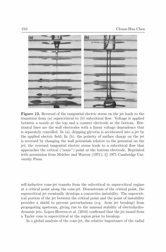
The essential role of tangential electric stress is illustrated by Figure 12(Melcher and Warren, 1971); see also the film by Melcher (1974). The po-larity of the free charge on the jet surface is controlled by a stack of wallelectrodes (horizontal lines in the figure). The induced surface charge takespositive or negative polarity, depending on the relative potential betweenthe wall electrodes and their corresponding location on the jet. The re-sulting tangential electric stress is either along (Figure 12a) or oppositeto (12b) the jet flow direction, leading to “supercritical” and “subcritical”flow, respectively. The 1D model employed by Melcher (1974) is essentiallythe same as Eq. 50, with the viscous stresses and surface charge convectionneglected and Eq. 50d replaced by a much simpler induction relationship.The neglection of viscous stresses reduces the system into a set of first orderwave equations with upstream and downstream wave velocities a− and a+in the convective frame traveling with the jet. In a supercritical flow rep-resented by Figure 12a, the jet velocity exceeds the upstream wave velocity(v > a−) so that downstream disturbances can not propagate upstream;In a subcritical flow (v < a−) represented by Figure 12b, disturbances can


ConvectiveAbsolute

Re

Ca

Figure 11. Absolute to convective instability transition for cone-jets. Solidcurves correspond to the theoretical predictions of the critical condition asa function of the charge parameter χ (Eq. 52), while discrete data pointsare the Reynolds and Capillary numbers estimated from cone-jets reportedin both electrospraying and electrospinning literature. Reprinted with per-mission from Lopez-Herrera et al. (2010), c© 2010 American Institute ofPhysics.

propagate in both directions so the flow is dependent on both upstreamand downstream conditions (Melcher and Warren, 1971). In this sense, thesubcritical/supercritical jet flow is analogous to subsonic/supersonic flow ofcompressible gas.

The supercritical concept was originally developed to explain the un-usually stable electrohydrodynamic jets with much longer breakup lengthcompared to their nonelectrical counterparts (Melcher and Warren, 1971).Ganan-Calvo (1997a) extended this line of work to include the convection ofsurface charge and more importantly, self-induction of electric fields from thefree surface charges (using a approach different from Eq. 50d). In Melcher(1974), the entire jet is either subcritical or supercritical when the surfacecharge is induced by wall electrodes. Ganan-Calvo (1997a) showed that a

210 Chuan-Hua Chen

(a) (b)

Figure 12. Reversal of the tangential electric stress on the jet leads to thetransition from (a) supercritical to (b) subcritical flow. Voltage is appliedbetween a nozzle at the top and a counter electrode at the bottom. Hor-izontal lines are the wall electrodes with a linear voltage dependence thatis separately conrolled. In (a), dripping glycerin is accelerated into a jet bythe applied electric field; In (b), the polarity of surface charge on the jetis reversed by changing the wall potentials relative to the potential on thejet; the reversed tangential electric stress leads to a subcritical flow thatapproaches the critical (“sonic”) point at the bottom electrode. Reprintedwith permission from Melcher and Warren (1971), c© 1971 Cambridge Uni-versity Press.

self-inductive cone-jet transits from the subcritical to supercritical regimeat a critical point along the cone-jet. Downstream of the critical point, thesupercritical jet eventually develops a convective instability. The supercrit-ical portion of the jet between the critical point and the point of instabilityprovides a shield to prevent perturbations (e.g. from jet breakup) frompropagating upstream, giving rise to the unusual stability of electrohydro-dynamic jets. Lopez-Herrera et al. (2010) confirmed that the jet issued froma Taylor cone is supercritical at the region prior to breakup.

In a global analysis of the cone-jet, the relative importance of the radial


to tangential electric stress,

ϑ =T err

T erz

∼ q2s/ε0qsE∞

=qs/ε0E∞

, (56)

is a function of location along the developing cone-jet. Close to the cone,tangential electric field dominates with a small surface charge density (ϑ1); Along the jet, radial electric field eventually dominates with increasingsurface charge density downstream (ϑ � 1). The surface charge density isdependent on the detailed cone-jet dynamics. In the form of Eq. 50 withnegligible gravity, qs is governed by the imposed electric field and flow rate(E∞Em

, QQm

) and the associated geometrical ( za , ξ), mechanical (We, Oh), and

electrical (α, β, χ) parameters. Because of the complex, global nature of theproblem, no controlling parameters (like Rae in Eq. 44) have emerged withappropriate scaling of the surface charge density in a developing cone-jet.

One possibility to reduce the complexity is to operate exactly at theminimum flow rate Q = Qm; accordingly, it is necessary for E = Em toobtain a steady cone-jet. Unfortunately, except for the empirical scalingEq. 49, the mechanism determining Qm is still unknown (Fernandez de laMora, 2007).

4.4 Pulsating cone-jet

The crucial role of the minimum flow rate (Qm) is apparent on theoperating diagram of steady cone-jets (Figure 9). In the previous section,we showed that a minimum flow rate (a critical Weber number) is necessaryfor the dripping to jetting transition (Eq. 55) if the electrohydrodynamicjet behaves analogously to its hydrodynamic counterpart. However, whenQ < Qm but E � Em, pulsating cone-jet sets in from a supported meniscuswhich does not have a clear hydrodynamic analogue.

Pulsating cone-jets are also observed on charged drops (e.g. Figure 8c);see Fernandez de la Mora (2007) for a comprehensive review. For an inviscidcharged drop in air, the lowest frequency of free drop oscillation (fd) is givenby Rayleigh (1882)

fd =4

π

√γ

ρd3

(1− q2

q2R

)∝ fc, (57)

where d is the diameter of the drop, q is the total charge on the surface,and

qR = π√8ε0γd3, (58)

is the Rayleigh limit for the maximum electrostatic charge allowed on astatic drop. Without any surface charge (q = 0), the frequency is simply

212 Chuan-Hua Chen

governed by the capillary-inertial process with a characteristic frequency offc =

√γ/ρd3. At the Rayleigh limit, electrostatic repulsion reduces the

effective surface tension to zero, leading to electrostatic fission of the drop.The electrostatic explosion can proceed through a fine fission mode via acone-jet (Figure 8c and Figure 13b), or a rough fission mode into a fewdrops of comparable size (Fernandez de la Mora, 2007).

(a) (b)

dd

dn

E

Ln

Figure 13. Analogy between pulsating cone-jets from a supported meniscusand an isolated drop: (a) The cone-jet transition under an external electricfield between a nozzle and a plate; (b) The cone-jet transition when a dropletexperiences electrostatic fission.

Fernandez de la Mora (1996) argued that the cone-jet pulsation on asupported meniscus is analogous to that on an isolated drop, as both re-sult from the redistribution of the excessive electrostatic charge to a largersurface area (Figure 13).6 When the time scale for cone-jet formation isshort compared to the duration of the cone-jet, which is the case for highconductivity liquid with rapid charge relaxation, the transient cone-jet isquasi-steady and is assumed to behave similarly to a steady cone-jet on asupported meniscus (Fernandez de la Mora, 1996). Since pulsation takesplace when the supply rate of liquid to the cone is less than the loss ratethrough the jet (Juraschek and Rollgen, 1998), a pulsating cone-jet will

6There are also many differences between steady and transient cone-jets, especially for

liquids with high viscosity and low conductivity; see Fernandez de la Mora (2007) for

details.


likely observe the minimum flow rate scaling (Fernandez de la Mora, 1996;Chen et al., 2006b). When the transient jet is on, the flow rate, jet diameterand electric current scale as (Fernandez de la Mora and Loscertales, 1994;Fernandez de la Mora, 1996; Barrero and Loscertales, 2007)

Qj ∼ γε

ρσ, (59a)

dj ∼(γε2

ρσ2

)1/3

, (59b)

ij ∼ g(ε)

(ε0γ

2

ρ

)1/2

, (59c)

where g(ε) accounts for the effects of liquid dielectric constant; For aqueoussolutions, g ≈ 18 (Fernandez de la Mora and Loscertales, 1994). The lifetimeof a transient cone-jet on an exploding drop can be obtained by integratingdt = −dq/i (Fernandez de la Mora, 1996),

Δtj ∼ Δq

ij∼ Δq

qR

qRij∼ 2

√2πΔq

g(ε)qR

√ρd3

γ∼√

ρd3

γ= τc, (60)

where Δtj is the time scale for a drop with surface charge approaching theRayleigh limit (qR) to emit enough charge (Δq) to reach a new electrostaticequilibrium. It is generally agreed that the mass loss due to electrostaticfission is negligible (order of 1%), but the charge loss is substantial (orderof 10%); see Fernandez de la Mora (1996). For water, the pre-factor inthe scaling of jet duration is close to 1 (Chen et al., 2006b). Interestingly,the jetting duration (Eq. 60) reduces to the capillary-inertial time scale(τc = 1/fc) which also sets the oscillation frequency of an uncharged drop(Eq. 57). If the pulsating cone-jet on a supported meniscus is analogous tothat on an exploding drop, the above scaling laws apply to both situationswith d taken as either the drop diameter (dd) or the anchoring diameter ofthe Taylor cone (e.g. the inner diameter of a non-wetting nozzle, dn).

We are now in a position to reconcile two different models for the pul-sating cone-jets by Marginean et al. (2006) and Chen et al. (2006b). At theonset of cone-jet pulsation, Marginean et al. (2006) observed that the pul-sation frequency on a support meniscus closely follows Eq. 57 with d equalto the anchoring diameter dn. However, the free oscillation frequency isindependent of the supplied flow rate Q, and this independence contradictswith the observations in Chen et al. (2006b) as well as empirical evidencesthat the emergence of cone-jet pulsation strongly depends on the flow rate(see Section 4.1).

214 Chuan-Hua Chen

Chen et al. (2006b) proposed a different model for the pulsation fre-quency, motivated by the hypothesis that cone-jet pulsations result when atransient jet discharges liquid mass at a rate (Qj) higher than the suppliedflow rate (Q). For each pulsation with a duration of Δtj , the volume ofliquid extracted scales as QjΔtj . By simple balance of mass flow suppliedto the cone and emitted by the jet, the pulsation frequency scales as (Chenet al., 2006b)

fj ∼ Q

QjΔtj∼ Q

Qmfc. (61)

In other words, cone-jet pulsations result when the mass flow is limited(“choked”) by upstream conditions. Note that for high conductivity fluid,the limiting factor leading to pulsation is the mass flow, not free charge,because surface charges can be generated at a rate governed the nearlyinstantaneous charge relaxation process. The pulsation model Eq. 61 hasbeen confirmed by Chen et al. (2006a,b) for cone-jet pulsations with a stableconical base (see insets in Figure 14).

Xu and Chen recently showed that both models are correct within theirapplicable regime (Xu, 2010). In Figure 14, both laws have been identifiedin the same system using flow rate as the only controlling parameter. Asthe flow rate increases, the frequency plateaus at relatively high flow rates.Microscopic imaging indicated that the oscillation modes at low and highflow rates are fundamentally different. At low flow rates, the Taylor coneonly deforms at the conical apex (“mass flow choking” regime); at highflow rates, the entire Taylor cone deforms significantly (“conical oscillation”regime). The demarcation between the two regimes is related to the mini-mum flow rate (Xu, 2010); For the conditions in Figure 14, Qm≈50 μL/haccording to Eq. 49.

• Q < Qm: The mass flow is choked upstream, and the pulsation fre-quency scales as f∼(Q/Qm)fc (Eq. 61). The linear dependence of thepulsation frequency on the flow rate is confirmed at small flow rates(Figure 14). The mass flow choking regime is unambiguously shownby cases with self-induced flow rate (Xu, 2010), which scales inverselywith the length of the slender nozzle (Chen et al., 2006b). The nozzlelength (Ln) is an upstream condition that will not change the conicaloscillation frequency (Eq. 57).

• Q � Qm: The conical base oscillates when ample liquid is supplied,and the frequency scales as f ∼ fc (Eq. 57). The fc∼ d−

32 scaling is

verified by Marginean et al. (2006) and confirmed by Xu (2010). Thediameter should be taken as that anchoring the conical base. For lowviscosity liquid, the anchoring diameter can become ambiguous and a


non-wettable nozzle (such as teflon) should be used to avoid excitingthe conical oscillation regime even at flow rates below Qm.

Note that the charge relaxation time (τe) is 3 μs in Figure 14, an orderof magnitude smaller than the 30 μs jetting duration (Δtj) predicted byEq. (60) and confirmed by experiments. Hence, the quasi-steady assumptionholds for the transient cone-jet discussed here.

Figure 14. Pulsation frequency as a function of the imposed (•) and in-duced (×) flow rate. The imposed flow rate is controlled by a syringe pump,while the electric-stress-induced flow rate is varied by the nozzle length.The glass nozzle has an inner diameter of 100 μm and an outer diameterof 160 μm; here the outer diameter is the anchoring diameter. Inset showsone duty cycle of pulsation for the imposed (top) and induced (bottom)flow rate. The applied voltage of 1.8 kV is slightly lower than the threshold(� 2.0 kV) for a steady cone-jet. The working fluid is doped ethylene glycolwith σ = 1.0 × 10−3 S/m, ε = 3.3 × 10−10 C/V·m, μ = 1.6 × 10−2 Pa·s,ρ=1.1× 103 kg/m3, and γ=4.5× 10−2 N/m.

The mechanistic understanding of pulsating cone-jets has practical im-plications for both electrohydrodynamic printing and miniaturized electro-spray. In both applications, slender nozzles with a diameter from 100 μmdown to 1 μm are routinely used. The viscous drag on the slender nozzlelimits the flow rate and leads to the regime of mass flow choking (Chenet al., 2006b). The intrinsic pulsations in the choking regime will influ-

216 Chuan-Hua Chen

ence the performance of both electroprinting and nanoelectrospray. Forexample, the highest speed of electrohydrodynamic printing is limited bythe intrinsic pulsation frequency (Chen et al., 2006a). The advantage ofnanoelectrospray over conventional electrospray diminishes with increasingflow rates (Schmidt et al., 2003); the critical flow rate is around the mini-mum flow rate (Eq. 49), suggesting a possible role of cone-jet pulsations innanoelectrospray.

5 Concluding Remarks

In this chapter, electrokinetic mixing flow and electrohydrodynamic cone-jet are reviewed as two model problems of electrohydrodynamic stability. Inboth cases, knowledge of the stability boundary is of practical interest foreither enhancing or suppressing the instability. Both problems are studiedusing the Ohmic model for leaky dielectrics with the assumptions of instan-taneous local charge relaxation and negligible diffusive current, which holdfor relatively conducting working fluids such as aqueous solutions.

The stability of electrokinetic mixing flow is relatively simple, owing inpart to the well-understood base state of a diffusive interface. Using thebulk-coupled model which accounts for the electric body forces induced byconductivity gradients, a large set of relevant experimental parameters canbe conveniently reduced to two controlling parameters: the electric Rayleighnumber relating the dynamic to dissipative processes which governs theonset of instability, and the electroviscous-to-electroosmotic velocity ratiowhich governs the onset of absolute instability.

The stability of electrohydrodynamic cone-jet is significantly more dif-ficult. Much of the difficulty is associated with the lack of a fundamentalunderstanding of the base state, i.e. the mechanisms leading to the formationof the Taylor cone-jet. Surface-coupled model is usually employed to relatethe electric and flow fields through the Maxwell stress, which now consistsof contributions from both free and bound charge due to conductivity andpermittivity gradients, respectively. Compared to its nonelectrical counter-part, the physics of electrohydrodynamic jets is enriched but complicatedby the electric field. The most useful guideline is still the electric field–flowrate operating diagram. Strategies to rationalize the operating diagram inthe framework of electrohydrodynamic stability have only been partiallysuccessful, e.g. within specific parametrical regimes of pulsating, spraying,or spinning cone-jets. Further research is required to understand key is-sues such as the origin of the minimum flow rate and the role of tangentialelectric stress before a unified theoretical picture is possible.


Bibliography

A. G. Bailey. Electrostatic Spraying of Liquids. Research Studies Press,1988.

A. Barrero and I. G. Loscertales. Micro- and nanoparticles via capillaryflows. Annu. Rev. Fluid Mech., 39:89–106, 2007.

J. C. Baygents and F. Baldessari. Electrohydrodynamic instability in athin fluid layer with an electrical conductivity gradient. Phys. Fluids,10:301–311, 1998.

H. C. Chang and L. Y. Yeo. Electrokinetically-Driven Microfluidics andNanofluidics. Cambridge University Press, 2010.

C. H. Chen, H. Lin, S. K. Lele, and J. G. Santiago. Convective and absoluteelectrokinetic instability with conductivity gradients. J. Fluid Mech.,524:263–303, 2005.

C. H. Chen, D. A. Saville, and I. A. Aksay. Electrohydrodynamic ‘drop-and-place’ particle deployment. Appl. Phys. Lett., 88:154104, 2006a.

C. H. Chen, D. A. Saville, and I. A. Aksay. Scaling laws for pulsed electro-hydrodynamic drop formation. Appl. Phys. Lett., 89:124103, 2006b.

M. Cloupeau and B. Prunet-Foch. Electrostatic spraying of liquids in cone-jet mode. J. Electrostat., 22:135–159, 1989.

M. Cloupeau and B. Prunet-Foch. Electrohydrodynamic spraying function-ing modes: a critical review. J. Aerosol Sci., 25:1021–1036, 1994.

D. Duft, T. Achtzehn, R. Muller, B. A. Huber, and T. Leisner. Coulombfission: Rayleigh jets from levitated microdroplets. Nature, 421:128,2003.

J. Eggers and E. Villermaux. Physics of liquid jets. Rep. Prog. Phys., 71:036601, 2008.

J. J. Feng. The stretching of an electrified non-Newtonian jet: a model forelectrospinning. Phys. Fluids, 14:3912–3926, 2002.

J. Fernandez de la Mora. On the outcome of the coulombic fission of acharged isolated drop. J. Colloid Interface Sci., 178:209–218, 1996.

J. Fernandez de la Mora. The fluid dynamics of Taylor cones. Annu. Rev.Fluid Mech., 39:217–243, 2007.

J. Fernandez de la Mora and I. G. Loscertales. The current emitted byhighly conducting Taylor cones. J. Fluid Mech., 260:155–184, 1994.

A. M. Ganan-Calvo. On the theory of electrohydrodynamically driven cap-illary jets. J. Fluid Mech., 335:165–188, 1997a.

A. M. Ganan-Calvo. Cone-jet analytical extension of Taylor’s electrostaticsolution and the asymptotic universal scaling laws in electrospraying.Phys. Rev. Lett., 79:217–220, 1997b.

A. M. Ganan-Calvo and J. M. Montanero. Revision of capillary cone-jetphysics: electrospray and flow focusing. Phys. Rev. E, 79:066305, 2009.

218 Chuan-Hua Chen

J. M. Grace and J. C. M. Marijnissen. A review of liquid atomization byelectrical means. J. Aerosol Sci., 25:1005–1019, 1994.

I. Hayati, A. I. Bailey, and Th. F. Tadros. Mechanism of stable jet formationin electrohydrodynamic atomization. Nature, 319:41–43, 1986.

J. F. Hoburg and J. R. Melcher. Internal electrohydrodynamic instabilityand mixing of fluids with orthogonal field and conductivity gradients. J.Fluid Mech., 73:333–351, 1976.

M. Hohman, M. Shin, G. C. Rutledge, and M. P. Brenner. Electrospinningand electrically forced jets. I. Stability theory. Phys. Fluids, 13:2201–2220, 2001a.

M. Hohman, M. Shin, G. C. Rutledge, and M. P. Brenner. Electrospinningand electrically forced jets. II. Applications. Phys. Fluids, 13:2221–2236,2001b.

P. Huerre and M. Rossi. Hydrodynamic instabilities in open flows. InC. Godreche and P. Manneville, editors, Hydrodynamics and NonlinearInstabilities. Cambridge University Press, 1998.

R. Juraschek and F. W. Rollgen. Pulsation phenomena during electrosprayionization. Int. J. Mass. Spectrom, 177:1–15, 1998.

P. Kebarle and U. H. Verkerk. Electrospray: from ions in solution to ionsin the gas phase, what we know now. Mass Spectrom. Rev., 28:898–917,2009.

L. G. Leal. Advanced Transport Phenomena. Cambridge University Press,2007.

W. G. Levich. Physicochemical Hydrodynamics. Prentice-Hall, 1962.H. Lin. Electrokinetic instability in microchannel flows: a review. Mech.

Res. Comm., 36:33–38, 2009.H. Lin, B. D. Storey, M. H. Oddy, C. H. Chen, and J.G. Santiago. Instability

of electrokinetic microchannel flows with conductivity gradients. Phys.Fluids, 16:1922–1935, 2004.

J. M. Lopez-Herrera, A. M. Ganan-Calvo, and M. A. Herrada. Linear sta-bility analysis of axisymmetric perturbations in imperfectly conductingliquid jets. Phys. Fluids, 17:034106, 2005.

J. M. Lopez-Herrera, P. Riesco-Chueca, and A. M. Ganan-Calvo. Absoluteto convective instability transition in charged liquid jets. Phys. Fluids,22:062002, 2010.

A. Manz, N. Graber, and H. M. Widmer. Miniaturized total chemical-analysis systems - a novel concept for chemical sensing. Sensors andActuators-B, 1:244–248, 1990.

I. Marginean, P. Nemes, L. Parvin, and A. Vertes. How much charge isthere on a pulsating Taylor cone? Appl. Phys. Lett., 89:064104, 2006.

I. Marginean, P. Nemes, and A. Vertes. Astable regime in electrosprays.Phys. Rev. E, 76:026320, 2007.


J. R. Melcher. Electric fields and moving media. IEEE Trans. Educ., E-17:100–110, 1974. This article describes the 16 mm film by J. R. Melcher,Electric Fields and Moving Media, produced by the Education Develop-ment Center, 39 Chapel Street, Newton, MA.

J. R. Melcher. Continuum Electromechanics. MIT Press, 1981.J. R. Melcher and W. J. Schwartz. Interfacial relaxation overstability in a

tangential electric field. Phys. Fluids, 11:2604–2616, 1968.J. R. Melcher and G. I. Taylor. Electrohydrodynamics: a review of the role

of interfacial shear stress. Annu. Rev. Fluid Mech., 1:111–146, 1969.J. R. Melcher and E. P. Warren. Electrohydrodynamics of a current-carrying

semi-insulating jet. J. Fluid Mech., 47:127–143, 1971.M. H. Oddy, J. G. Santiago, and J. C. Mikkelsen. Electrokinetic instability

micromixing. Anal. Chem., 73:5822–5832, 2001.W. K. H. Panofsky and M. Phillips. Classical Electricity and Magnetism.

Addison-Wesley, 2nd edition, 1962. Dover, 2005.J. U. Park, M. Hardy, S. J. Kang, K. Barton, K. Adair, D. K. Mukhopad-

hyay, C. Y. Lee, M. S. Strano, A. G. Alleyne, J. G. Georgiadis, P. M. Fer-reira, and J.A. Rogers. High-resolution electrohydrodynamic jet printing.Nat. Mater., 6:782–789, 2007.

J. D. Posner and J. G. Santiago. Convective instability of electrokineticflows in a cross-shaped microchannel. J. Fluid Mech., 555:1–42, 2006.

Lord Rayleigh. On the instability of jets. Proc. London Math. Soc., 10:4–13, 1879.

Lord Rayleigh. On the equilibrium of liquid conducting masses charged withelectricity. Philos. Mag., 14:184–186, 1882.

D. H. Reneker, A. L. Yarin, E. Zussman, and H. Xu. Electrospinning ofnanofibers from polymer solutions and melts. Adv. Appl. Mech., 41:43–195, 2007.

D. A. Saville. Electrohydrodynamics: the Taylor-Melcher leaky dielectricmodel. Annu. Rev. Fluid Mech., 29:27–64, 1997.

P. J. Schmid and D. S. Henningson. Stability and Transition in Shear Flows.Springer, 2001.

A. Schmidt, M. Karas, and T. Dulcks. Effect of different solution flow rateson analyte ion signals in nano-ESI MS, or: when does ESI turn intonano-ESI? J. Am. Soc. Mass Spectrom., 14:492–500, 2003.

D. P. H. Smith. The electrohydodynamic atomization of liquids. IEEETrans. Indus. Appl., IA-22:527–535, 1986.

H. A. Stone, A. D. Stroock, , and A. Ajdari. Engineering flows in smalldevices: microfluidics toward a lab-on-a-chip. Annu. Rev. Fluid Mech.,36:381–411, 2004.

G. I. Taylor. Disintegration of water drops in an electric field. Proc. R. Soc.London A, 280:383–397, 1964.

220 Chuan-Hua Chen

M. S. Wilm and M. Mann. Electrospray and Taylor-cone theory, Dole’sbeam of macromolecules at last? Int. J. Mass Spectrom., 136:167–180,1994.

S. Xu. Operating regimes of self-regulated electrohydrodynamic cone-jets.Master’s thesis, Duke University, 2010.

O. Yogi, T. Kawakami, M. Yamauchi, J.Y. Ye, and M. Ishikawa. On-demanddroplet spotter for preparing pico- to femtoliter droplets on surfaces.Anal. Chem., 73:1896–1902, 2001.

J. Zeng and T. Korsmeyer. Principles of droplet electrohydrodynamics forlab-on-a-chip. Lab Chip, 4:265–277, 2004.

electrohydrodynamic stability

Documents