electrical networks and algebraic graph theory: models...
TRANSCRIPT
1
Electrical Networks and Algebraic Graph Theory:Models, Properties, and Applications
Florian Dorfler, Member, IEEE, John W. Simpson-Porco, Member, IEEE, and Francesco Bullo, Fellow, IEEE
Abstract—Algebraic graph theory is a cornerstone in thestudy of electrical networks ranging from miniature integratedcircuits to continental-scale power systems. Conversely, manyfundamental results of algebraic graph theory were laid outby early electrical circuit analysts. In this paper we surveysome fundamental and historic as well as recent results onhow algebraic graph theory informs electrical network analysis,dynamics, and design. In particular, we review the algebraic andspectral properties of graph adjacency, Laplacian, incidence, andresistance matrices and how they relate to the analysis, network-reduction, and dynamics of certain classes of electrical networks.We study these relations for models of increasing complexityranging from static resistive DC circuits, over dynamic RLCcircuits, to nonlinear AC power flow. We conclude this paper bypresenting a set of fundamental open questions at the intersectionof algebraic graph theory and electrical networks.
I. INTRODUCTION
The study of electrical networks, the theory of graphs,and their associated matrices share a long and rich historyof synergy and joint development. Starting from the founda-tional classical work by Gustav Kirchhoff [87], modeling andanalysis of electric circuits has motivated the birth and thedevelopment of a broad range of graph-theoretical conceptsand certain classes of matrices. Vice-versa, algebraic graphtheory concepts and constructions have enabled fundamentaladvances in the theory of electrical networks. As is wellknown, it is in graph-theoretical language that Kirchhoff’s lawsare most succinctly and powerfully expressed, and it is viamatrix theory that the discrete nature of graphs is most pow-erfully analyzed. To this day, graph theory, matrix analysis,and electrical networks inspire and enrich one another.
In this paper we survey some fundamental and historicas well as recent results on how algebraic graph theoryinforms electrical network analysis, dynamics, and design. Inparticular, we review the algebraic and spectral properties ofgraph adjacency, Laplacian, Metzler, incidence, and effectiveresistance matrices; we review the basic notions from algebraicpotential theory, including cycle and cutset spaces.
F. Dorfler is with the Automatic Control Laboratory, ETH Zurich, 8092Zurich, Switzerland. Email: [email protected].
J. W. Simpson-Porco is with the Department of Electrical and ComputerEngineering, University of Waterloo, Waterloo, ON N2L 3G1, Canada. Email:[email protected].
F. Bullo is with the Center for Control, Dynamical Systems and Com-putation, University of California, Santa Barbara, CA 93106, USA. Email:[email protected].
This work was supported in part by the SNF AP Energy Grant #160573, theU.S. Department of Energy (DOE) Solar Energy Technologies Office underContract No. DE-EE0000-1583, by the National Science and EngineeringCouncil of Canada Discovery RGPIN-2017-04008, and by ETH Zurich funds.
We then study general models of electrical networks, start-ing from elementary models and building up to a prototypicalcircuit, with several instructive special cases. Our proposedprototypical circuit is a Π-line-coupled RC circuit with non-linear sources and loads. This prototypical nonlinear RLCcircuit has numerous interesting features. First, our prototypi-cal circuit generalizes the widely-studied resistive circuit andfeatures rich dynamical behaviors, including synchronizationand consensus behaviors. Second, power system network mod-elling is essentially based on this circuit (Π-line transmissionmodels, charging capacitors at the buses, and ZIP loads,including modern constant-power devices). Third and final, itshowcases popular energy-based, power-based, and compart-mental modeling approaches, and it is sufficiently general toadmit a variety of graph-theoretic analysis approaches.
Based on algebraic graph theory methods, we then study theanalysis, network-reduction, and dynamics of our prototypicalcircuit and its variations, in linear and nonlinear as well asstatic and dynamic settings. Thereby we consider models of in-creasing complexity ranging from static resistive circuits, overdynamic RLC networks, to nonlinear AC power flow models.We motivate our treatment with a few interesting examples,review a few fundamental and historic results in a tutorialexposition, and also showcase related recent developments.Our focus is on static and dynamic analysis of DC circuits,except for Section VI-B where we explicitly focus on steady-state analysis of AC circuits through the lens of graph theory.
It is important to clarify that this article does not aim to becomprehensive in its scope, nor does it present multiple view-points on the given material, as both algebraic graph theoryand electrical circuits are mature and broadly developed fields.In the context of algebraic graph theory, we refer interestedreaders to the textbooks [16], [19], [72] and, for example, thesurveys [102], [97], [17]. There are numerous complementaryviewpoints on electrical network modeling and analysis. Wemention the well-established linear network theory [6], [144],[101], [145]; classical network analysis in the nonlinear setting[37], [36], [124]; the signals, systems, and control view-point [4]; the behavioral approach [148] and its applicationto circuits [149]; energy-based Port-Hamiltonian approaches[135], [104], [133], [95]; and power-based Brayton-Moserapproaches [25], [26], [83], [85], [84] among others. Ourexposition and treatment highlights the algebraic graph theoryperspective on electrical networks, with examples colored byour own research interests and experiences.
The remainder of the paper is organized as follows. Webegin with a set of motivating examples in Section II thatoutline the themes of the paper. Section III briefly reviews
2
relevant results of algebraic theory. In Section IV we presentthe general modeling of electrical networks based on thelanguage of graph theory and also introduce a prototypicalnetwork model that we will frequently revisit in the courseof the paper. Section V showcases the tools of algebraicgraph theory to analyze the structure and dynamics of linearelectrical networks, and Section VI addresses the nonlinearcase. Finally, Section VII concludes the paper and outlines afew open and worthwhile research directions at the intersectionof electrical networks and algebraic graph theory.
II. MOTIVATING EXAMPLES
We begin by laying out a set of motivating examples withapparently complex behavior, whose analysis becomes crispand clear by using the tools of algebraic graph theory. Wewill revisit each of these examples in the course of the paper.
A. Synchronization of resonant LC tanks
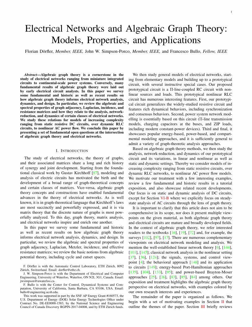
Consider the electrical network in Figure 1 consisting ofidentical resonant tank circuits interconnected through resistivebranches. Each tank circuit consists of a parallel connection ofan inductor and a capacitor with identical values of inductance` > 0 and capacitance c > 0.
r` c
rr
r
` c` c ` c
Fig. 1. Network of resistively interconnected `c-tanks; image courtesy of [27].
As known from undergraduate engineering education, eachtank circuit in isolation exhibits harmonic oscillations withnatural frequency ω0 = 1/
√`c and phase and amplitude de-
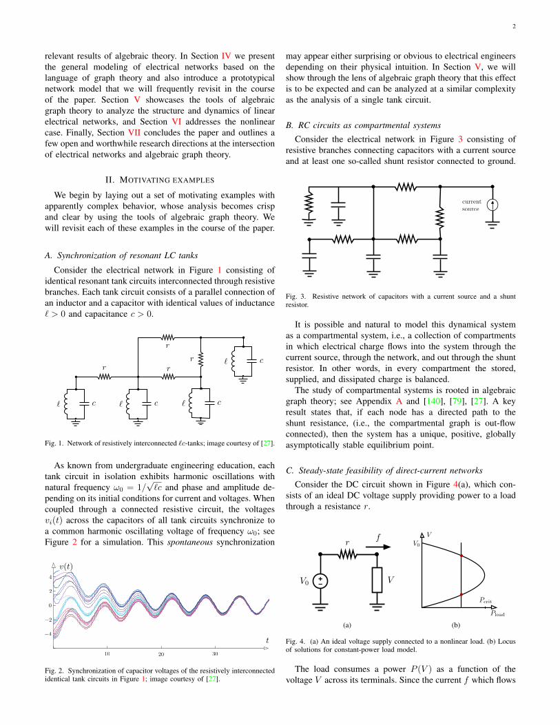
pending on its initial conditions for current and voltages. Whencoupled through a connected resistive circuit, the voltagesvi(t) across the capacitors of all tank circuits synchronize toa common harmonic oscillating voltage of frequency ω0; seeFigure 2 for a simulation. This spontaneous synchronization
t
v(t)
10 20 30
−4
−2
0
2
4
Fig. 2. Synchronization of capacitor voltages of the resistively interconnectedidentical tank circuits in Figure 1; image courtesy of [27].
may appear either surprising or obvious to electrical engineersdepending on their physical intuition. In Section V, we willshow through the lens of algebraic graph theory that this effectis to be expected and can be analyzed at a similar complexityas the analysis of a single tank circuit.
B. RC circuits as compartmental systems
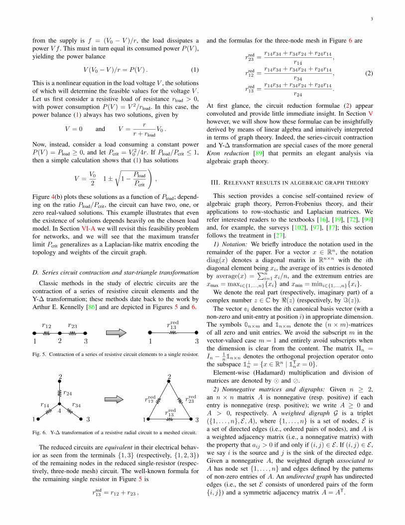
Consider the electrical network in Figure 3 consisting ofresistive branches connecting capacitors with a current sourceand at least one so-called shunt resistor connected to ground.
currentsource
Fig. 3. Resistive network of capacitors with a current source and a shuntresistor.
It is possible and natural to model this dynamical systemas a compartmental system, i.e., a collection of compartmentsin which electrical charge flows into the system through thecurrent source, through the network, and out through the shuntresistor. In other words, in every compartment the stored,supplied, and dissipated charge is balanced.
The study of compartmental systems is rooted in algebraicgraph theory; see Appendix A and [140], [79], [27]. A keyresult states that, if each node has a directed path to theshunt resistance, (i.e., the compartmental graph is out-flowconnected), then the system has a unique, positive, globallyasymptotically stable equilibrium point.
C. Steady-state feasibility of direct-current networks
Consider the DC circuit shown in Figure 4(a), which con-sists of an ideal DC voltage supply providing power to a loadthrough a resistance r.
V=+V0
rf
(a)
V
Pload
Pcrit
V0
(b)
Fig. 4. (a) An ideal voltage supply connected to a nonlinear load. (b) Locusof solutions for constant-power load model.
The load consumes a power P (V ) as a function of thevoltage V across its terminals. Since the current f which flows
3
from the supply is f = (V0 − V )/r, the load dissipates apower V f . This must in turn equal its consumed power P (V ),yielding the power balance
V (V0 − V )/r = P (V ) . (1)
This is a nonlinear equation in the load voltage V , the solutionsof which will determine the feasible values for the voltage V .Let us first consider a resistive load of resistance rload > 0,with power consumption P (V ) = V 2/rload. In this case, thepower balance (1) always has two solutions, given by
V = 0 and V =r
r + rloadV0 .
Now, instead, consider a load consuming a constant powerP (V ) = Pload ≥ 0, and let Pcrit = V 2
0 /4r. If Pload/Pcrit ≤ 1,then a simple calculation shows that (1) has solutions
V =V0
2
(1±
√1− Pload
Pcrit
),
Figure 4(b) plots these solutions as a function of Pload; depend-ing on the ratio Pload/Pcrit, the circuit can have two, one, orzero real-valued solutions. This example illustrates that eventhe existence of solutions depends heavily on the chosen loadmodel. In Section VI-A we will revisit this feasibility problemfor networks, and we will see that the maximum transferlimit Pcrit generalizes as a Laplacian-like matrix encoding thetopology and weights of the circuit graph.
D. Series circuit contraction and star-triangle transformation
Classic methods in the study of electric circuits are thecontraction of a series of resistive circuit elements and theY-∆ transformation; these methods date back to the work byArthur E. Kennelly [86] and are depicted in Figures 5 and 6.
308 8
8 8
1 13 32
r12 r23 rred13
Fig. 5. Contraction of a series of resistive circuit elements to a single resistor.
30
88
8
8
8
81 1
22
334
r14
r24
r34rred12 rred
23
rred13
Fig. 6. Y-∆ transformation of a resistive radial circuit to a meshed circuit.
The reduced circuits are equivalent in their electrical behav-ior as seen from the terminals {1, 3} (respectively, {1, 2, 3})of the remaining nodes in the reduced single-resistor (respec-tively, three-node mesh) circuit. The well-known formula forthe remaining single resistor in Figure 5 is
rred13 = r12 + r23 ,
and the formulas for the three-node mesh in Figure 6 are
rred23 =
r14r34 + r34r24 + r24r14
r14,
rred12 =
r14r34 + r34r24 + r24r14
r34,
rred13 =
r14r34 + r34r24 + r24r14
r24.
(2)
At first glance, the circuit reduction formulae (2) appearconvoluted and provide little immediate insight. In Section Vhowever, we will show how these formulae can be insightfullyderived by means of linear algebra and intuitively interpretedin terms of graph theory. Indeed, the series-circuit contractionand Y-∆ transformation are special cases of the more generalKron reduction [89] that permits an elegant analysis viaalgebraic graph theory.
III. RELEVANT RESULTS IN ALGEBRAIC GRAPH THEORY
This section provides a concise self-contained review ofalgebraic graph theory, Perron-Frobenius theory, and theirapplications to row-stochastic and Laplacian matrices. Werefer interested readers to the textbooks [16], [19], [72], [99]and, for example, the surveys [102], [97], [17]; this sectionfollows the treatment in [27].
1) Notation: We briefly introduce the notation used in theremainder of the paper. For a vector x ∈ Rn, the notationdiag(x) denotes a diagonal matrix in Rn×n with the ithdiagonal element being xi, the average of its entries is denotedby average(x) =
∑ni=1 xi/n, and the extremum entries are
xmax = maxi∈{1,...,n}{xi} and xmin = mini∈{1,...,n}{xi}.We denote the real part (respectively, imaginary part) of a
complex number z ∈ C by <(z) (respectively, by =(z)).The vector ei denotes the ith canonical basis vector (with a
non-zero and unit-entry at position i) in appropriate dimension.The symbols 0n×m and 1n×m denote the (n ×m)-matricesof all zero and unit entries. We avoid the subscript m in thevector-valued case m = 1 and entirely avoid subscripts whenthe dimension is clear from the content. The matrix Πn =In − 1
n1n×n denotes the orthogonal projection operator ontothe subspace 1⊥n = {x ∈ Rn | 1T
nx = 0}.Element-wise (Hadamard) multiplication and division of
matrices are denoted by � and �.2) Nonnegative matrices and digraphs: Given n ≥ 2,
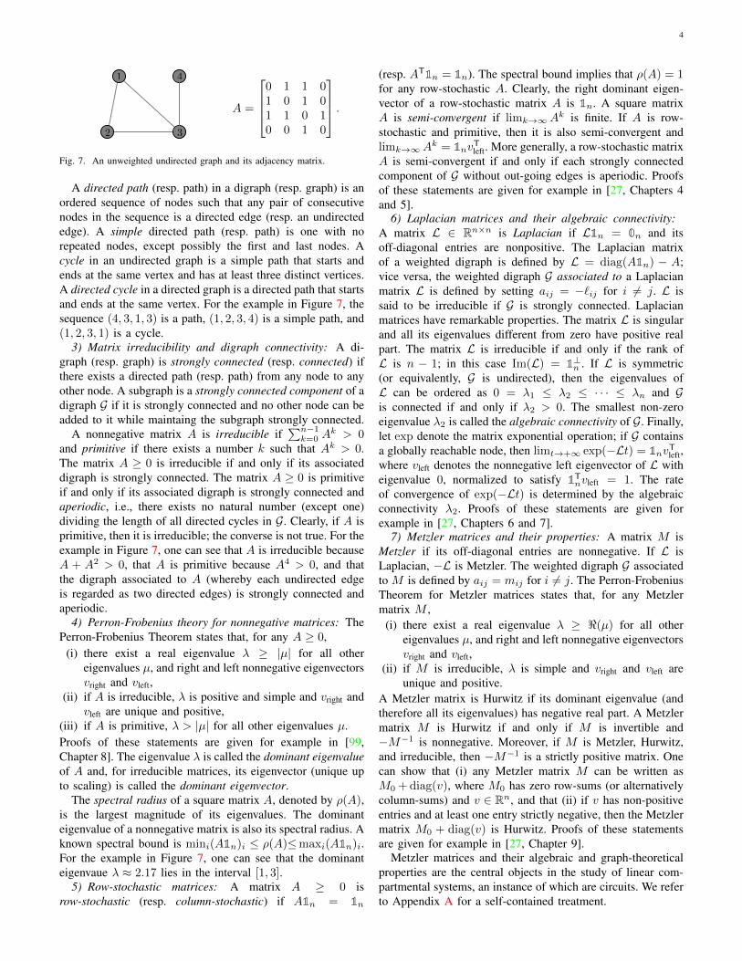
an n × n matrix A is nonnegative (resp. positive) if eachentry is nonnegative (resp. positive); we write A ≥ 0 andA > 0, respectively. A weighted digraph G is a triplet({1, . . . , n}, E , A), where {1, . . . , n} is a set of nodes, E isa set of directed edges (i.e., ordered pairs of nodes), and A isa weighted adjacency matrix (i.e., a nonnegative matrix) withthe property that aij > 0 if and only if (i, j) ∈ E . If (i, j) ∈ E ,we say i is the source and j is the sink of the directed edge.Given a nonnegative A, the weighted digraph associated toA has node set {1, . . . , n} and edges defined by the patternsof non-zero entries of A. An undirected graph has undirectededges (i.e., the set E consists of unordered pairs of the form{i, j}) and a symmetric adjacency matrix A = AT.
4
1
2 3
4
A =
0 1 1 01 0 1 01 1 0 10 0 1 0
.
Fig. 7. An unweighted undirected graph and its adjacency matrix.
A directed path (resp. path) in a digraph (resp. graph) is anordered sequence of nodes such that any pair of consecutivenodes in the sequence is a directed edge (resp. an undirectededge). A simple directed path (resp. path) is one with norepeated nodes, except possibly the first and last nodes. Acycle in an undirected graph is a simple path that starts andends at the same vertex and has at least three distinct vertices.A directed cycle in a directed graph is a directed path that startsand ends at the same vertex. For the example in Figure 7, thesequence (4, 3, 1, 3) is a path, (1, 2, 3, 4) is a simple path, and(1, 2, 3, 1) is a cycle.
3) Matrix irreducibility and digraph connectivity: A di-graph (resp. graph) is strongly connected (resp. connected) ifthere exists a directed path (resp. path) from any node to anyother node. A subgraph is a strongly connected component of adigraph G if it is strongly connected and no other node can beadded to it while maintaing the subgraph strongly connected.
A nonnegative matrix A is irreducible if∑n−1k=0 A
k > 0and primitive if there exists a number k such that Ak > 0.The matrix A ≥ 0 is irreducible if and only if its associateddigraph is strongly connected. The matrix A ≥ 0 is primitiveif and only if its associated digraph is strongly connected andaperiodic, i.e., there exists no natural number (except one)dividing the length of all directed cycles in G. Clearly, if A isprimitive, then it is irreducible; the converse is not true. For theexample in Figure 7, one can see that A is irreducible becauseA + A2 > 0, that A is primitive because A4 > 0, and thatthe digraph associated to A (whereby each undirected edgeis regarded as two directed edges) is strongly connected andaperiodic.
4) Perron-Frobenius theory for nonnegative matrices: ThePerron-Frobenius Theorem states that, for any A ≥ 0,
(i) there exist a real eigenvalue λ ≥ |µ| for all othereigenvalues µ, and right and left nonnegative eigenvectorsvright and vleft,
(ii) if A is irreducible, λ is positive and simple and vright andvleft are unique and positive,
(iii) if A is primitive, λ > |µ| for all other eigenvalues µ.Proofs of these statements are given for example in [99,Chapter 8]. The eigenvalue λ is called the dominant eigenvalueof A and, for irreducible matrices, its eigenvector (unique upto scaling) is called the dominant eigenvector.
The spectral radius of a square matrix A, denoted by ρ(A),is the largest magnitude of its eigenvalues. The dominanteigenvalue of a nonnegative matrix is also its spectral radius. Aknown spectral bound is mini(A1n)i ≤ ρ(A)≤maxi(A1n)i.For the example in Figure 7, one can see that the dominanteigenvaue λ ≈ 2.17 lies in the interval [1, 3].
5) Row-stochastic matrices: A matrix A ≥ 0 isrow-stochastic (resp. column-stochastic) if A1n = 1n
(resp. AT1n = 1n). The spectral bound implies that ρ(A) = 1for any row-stochastic A. Clearly, the right dominant eigen-vector of a row-stochastic matrix A is 1n. A square matrixA is semi-convergent if limk→∞Ak is finite. If A is row-stochastic and primitive, then it is also semi-convergent andlimk→∞Ak = 1nvTleft. More generally, a row-stochastic matrixA is semi-convergent if and only if each strongly connectedcomponent of G without out-going edges is aperiodic. Proofsof these statements are given for example in [27, Chapters 4and 5].
6) Laplacian matrices and their algebraic connectivity:A matrix L ∈ Rn×n is Laplacian if L1n = 0n and itsoff-diagonal entries are nonpositive. The Laplacian matrixof a weighted digraph is defined by L = diag(A1n) − A;vice versa, the weighted digraph G associated to a Laplacianmatrix L is defined by setting aij = −`ij for i 6= j. L issaid to be irreducible if G is strongly connected. Laplacianmatrices have remarkable properties. The matrix L is singularand all its eigenvalues different from zero have positive realpart. The matrix L is irreducible if and only if the rank ofL is n − 1; in this case Im(L) = 1⊥n . If L is symmetric(or equivalently, G is undirected), then the eigenvalues ofL can be ordered as 0 = λ1 ≤ λ2 ≤ · · · ≤ λn and Gis connected if and only if λ2 > 0. The smallest non-zeroeigenvalue λ2 is called the algebraic connectivity of G. Finally,let exp denote the matrix exponential operation; if G containsa globally reachable node, then limt→+∞ exp(−Lt) = 1nvTleft,where vleft denotes the nonnegative left eigenvector of L witheigenvalue 0, normalized to satisfy 1T
nvleft = 1. The rateof convergence of exp(−Lt) is determined by the algebraicconnectivity λ2. Proofs of these statements are given forexample in [27, Chapters 6 and 7].
7) Metzler matrices and their properties: A matrix M isMetzler if its off-diagonal entries are nonnegative. If L isLaplacian, −L is Metzler. The weighted digraph G associatedto M is defined by aij = mij for i 6= j. The Perron-FrobeniusTheorem for Metzler matrices states that, for any Metzlermatrix M ,
(i) there exist a real eigenvalue λ ≥ <(µ) for all othereigenvalues µ, and right and left nonnegative eigenvectorsvright and vleft,
(ii) if M is irreducible, λ is simple and vright and vleft areunique and positive.
A Metzler matrix is Hurwitz if its dominant eigenvalue (andtherefore all its eigenvalues) has negative real part. A Metzlermatrix M is Hurwitz if and only if M is invertible and−M−1 is nonnegative. Moreover, if M is Metzler, Hurwitz,and irreducible, then −M−1 is a strictly positive matrix. Onecan show that (i) any Metzler matrix M can be written asM0 + diag(v), where M0 has zero row-sums (or alternativelycolumn-sums) and v ∈ Rn, and that (ii) if v has non-positiveentries and at least one entry strictly negative, then the Metzlermatrix M0 + diag(v) is Hurwitz. Proofs of these statementsare given for example in [27, Chapter 9].
Metzler matrices and their algebraic and graph-theoreticalproperties are the central objects in the study of linear com-partmental systems, an instance of which are circuits. We referto Appendix A for a self-contained treatment.
5
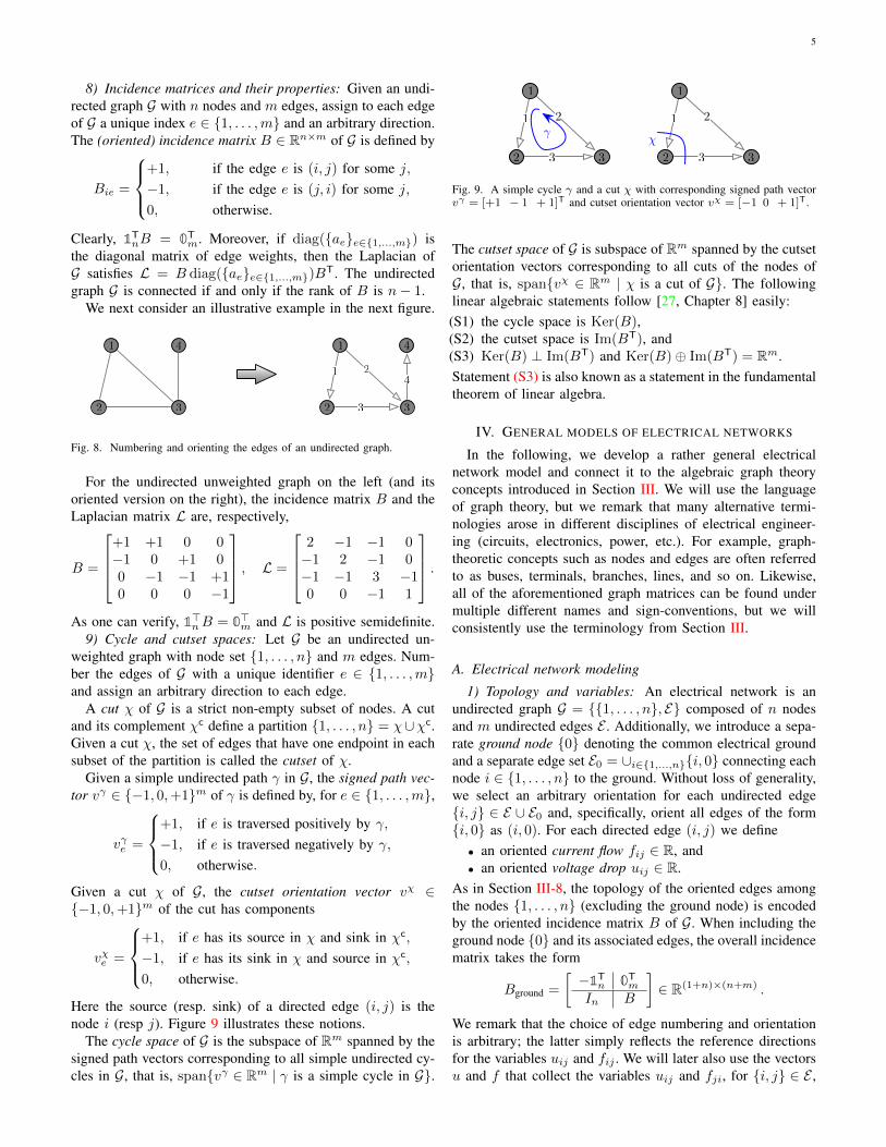
8) Incidence matrices and their properties: Given an undi-rected graph G with n nodes and m edges, assign to each edgeof G a unique index e ∈ {1, . . . ,m} and an arbitrary direction.The (oriented) incidence matrix B ∈ Rn×m of G is defined by
Bie =
+1, if the edge e is (i, j) for some j,−1, if the edge e is (j, i) for some j,0, otherwise.
Clearly, 1TnB = 0T
m. Moreover, if diag({ae}e∈{1,...,m}) isthe diagonal matrix of edge weights, then the Laplacian ofG satisfies L = B diag({ae}e∈{1,...,m})BT. The undirectedgraph G is connected if and only if the rank of B is n− 1.
We next consider an illustrative example in the next figure.
1
2 3
1
2 3
1 2
3
4 4
4
Fig. 8. Numbering and orienting the edges of an undirected graph.
For the undirected unweighted graph on the left (and itsoriented version on the right), the incidence matrix B and theLaplacian matrix L are, respectively,
B =
+1 +1 0 0−1 0 +1 00 −1 −1 +10 0 0 −1
, L =
2 −1 −1 0−1 2 −1 0−1 −1 3 −10 0 −1 1
.
As one can verify, 1>nB = 0>m and L is positive semidefinite.9) Cycle and cutset spaces: Let G be an undirected un-
weighted graph with node set {1, . . . , n} and m edges. Num-ber the edges of G with a unique identifier e ∈ {1, . . . ,m}and assign an arbitrary direction to each edge.
A cut χ of G is a strict non-empty subset of nodes. A cutand its complement χc define a partition {1, . . . , n} = χ∪χc.Given a cut χ, the set of edges that have one endpoint in eachsubset of the partition is called the cutset of χ.
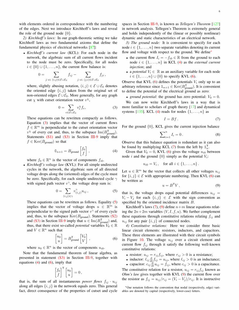
Given a simple undirected path γ in G, the signed path vec-tor vγ ∈ {−1, 0,+1}m of γ is defined by, for e ∈ {1, . . . ,m},
vγe =
+1, if e is traversed positively by γ,−1, if e is traversed negatively by γ,0, otherwise.
Given a cut χ of G, the cutset orientation vector vχ ∈{−1, 0,+1}m of the cut has components
vχe =
+1, if e has its source in χ and sink in χc,
−1, if e has its sink in χ and source in χc,
0, otherwise.
Here the source (resp. sink) of a directed edge (i, j) is thenode i (resp j). Figure 9 illustrates these notions.
The cycle space of G is the subspace of Rm spanned by thesigned path vectors corresponding to all simple undirected cy-cles in G, that is, span{vγ ∈ Rm | γ is a simple cycle in G}.
1
2 3
1 2
3
�
1
2 3
1 2
3
�
Fig. 9. A simple cycle γ and a cut χ with corresponding signed path vectorvγ = [+1 − 1 + 1]T and cutset orientation vector vχ = [−1 0 + 1]T.
The cutset space of G is subspace of Rm spanned by the cutsetorientation vectors corresponding to all cuts of the nodes ofG, that is, span{vχ ∈ Rm | χ is a cut of G}. The followinglinear algebraic statements follow [27, Chapter 8] easily:(S1) the cycle space is Ker(B),(S2) the cutset space is Im(BT), and(S3) Ker(B) ⊥ Im(BT) and Ker(B)⊕ Im(BT) = Rm.Statement (S3) is also known as a statement in the fundamentaltheorem of linear algebra.
IV. GENERAL MODELS OF ELECTRICAL NETWORKS
In the following, we develop a rather general electricalnetwork model and connect it to the algebraic graph theoryconcepts introduced in Section III. We will use the languageof graph theory, but we remark that many alternative termi-nologies arose in different disciplines of electrical engineer-ing (circuits, electronics, power, etc.). For example, graph-theoretic concepts such as nodes and edges are often referredto as buses, terminals, branches, lines, and so on. Likewise,all of the aforementioned graph matrices can be found undermultiple different names and sign-conventions, but we willconsistently use the terminology from Section III.
A. Electrical network modeling
1) Topology and variables: An electrical network is anundirected graph G = {{1, . . . , n}, E} composed of n nodesand m undirected edges E . Additionally, we introduce a sepa-rate ground node {0} denoting the common electrical groundand a separate edge set E0 = ∪i∈{1,...,n}{i, 0} connecting eachnode i ∈ {1, . . . , n} to the ground. Without loss of generality,we select an arbitrary orientation for each undirected edge{i, j} ∈ E ∪ E0 and, specifically, orient all edges of the form{i, 0} as (i, 0). For each directed edge (i, j) we define• an oriented current flow fij ∈ R, and• an oriented voltage drop uij ∈ R.
As in Section III-8, the topology of the oriented edges amongthe nodes {1, . . . , n} (excluding the ground node) is encodedby the oriented incidence matrix B of G. When including theground node {0} and its associated edges, the overall incidencematrix takes the form
Bground =
[−1T
n 0Tm
In B
]∈ R(1+n)×(n+m) .
We remark that the choice of edge numbering and orientationis arbitrary; the latter simply reflects the reference directionsfor the variables uij and fij . We will later also use the vectorsu and f that collect the variables uij and fji, for {i, j} ∈ E ,
6
with elements ordered in correspondence with the numberingof the edges. Next we introduce Kirchhoff’s laws and revealthe role of the ground node {0}.
2) Kirchhoff’s laws: In our graph-theoretic setting we takeKirchhoff laws as two fundamental axioms that define thefundamental physics of electrical networks [87]:• Kirchhoff’s current law (KCL): For each node in the
network, the algebraic sum of all current flows incidentto the node must be zero. Specifically, for all nodesi ∈ {0} ∪ {1, . . . , n}, the current flow balance is:
0 =∑
j s.t. (i,j)∈E∪E0fij −
∑
j s.t. (j,i)∈E∪E0fji ,
where, slightly abusing notation, (i, j) ∈ E ∪ E0 denotesthe oriented edge {i, j} taken from the original set ofnon-oriented edges E ∪E0. More generally, for any graphcut χ with cutset orientation vector vχ,
0 =∑
e∈E∪E0vχe fe, (3)
These equations can be rewritten compactly as follows.Equation (3) implies that the vector of current flowsf ∈ Rm is perpendicular to the cutset orientation vectorvχ of every cut and, thus, to the subspace Im(BT
ground).Statements (S1) and (S3) in Section III-9 imply thatf ∈ Ker(Bground) so that
0n+1 = Bground
[f0
f
], (4)
where f0 ∈ Rn is the vector of components fi0.• Kirchhoff’s voltage law (KVL): For all simple undirected
cycles in the network, the algebraic sum of all directedvoltage drops along the (oriented) edges of the cycle mustbe zero. Specifically, for each simple undirected cycle γwith signed path vector vγ , the voltage drop sum is:
0 =∑
(i,j)∈γvγ(i,j)uij , (5)
These equations can be rewritten as follows. Equality (5)implies that the vector of voltage drops u ∈ Rm isperpendicular to the signed path vector vγ of every cycleand, thus, to the subspace Ker(Bground). Statements (S2)and (S3) in Section III-9 imply that u ∈ Im(BT
ground) and,thus, that there exist so-called potential variables V0 ∈ Rand V ∈ Rn such that[
u0
u
]= BT
ground
[V0
V
], (6)
where u0 ∈ Rn is the vector of components ui0.Note that the fundamental theorem of linear algebra, as
presented in statement (S3) in Section III-9, together withequations (4) and (6), imply that
[f0
f
]T [u0
u
]= 0 ,
that is, the sum of all instantaneous power flows fij · uijalong all edges {i, j} in the network equals zero. This generalfact, direct consequence of the properties of cutset and cycle
spaces in Section III-9, is known as Tellegen’s Theorem [127]in network analysis. Tellegen’s Theorem is extremely generaland holds independently of the (linear or possibly nonlinear)dynamic and static characteristics of an electrical network.
3) The ground node: It is convenient to specify for eachnode i ∈ {1, . . . , n} two separate variables denoting its currentflow and voltage with respect to the ground. We define∗
• the current flow Ii = −fi0 ∈ R from the ground to eachnode i ∈ {1, . . . , n} in KCL (4) as the external currentinjection; and
• a potential Vi ∈ R as an auxiliary variable for each nodei ∈ {1, . . . , n} ∪ {0} to specify KVL (6).
Observe that KVL (6) defines the potentials Vi only up to anarbitrary reference since 1n+1 ∈ Ker(BT
ground). It is convenientto define the potential of the electrical ground as zero:• ground potential: the ground has zero potential: V0 = 0.We can now write Kirchhoff’s laws in a way that is
more familiar to scholars of graph theory [17] and dynamicalsystems [135]. KCL (4) reads for nodes {1, . . . , n} as
I = Bf . (7)
For the ground {0}, KCL gives the current injection balance∑n
i=1Ii = 0 . (8)
Observe that this balance equation is redundant as it can alsobe found by multiplying KCL (7) from the left by 1T
n.Given that V0 = 0, KVL (6) gives the voltage ui0 between
node i and the ground {0} simply as the potential Vi:
ui0 = Vi , for all i ∈ {1, . . . , n} .Let u ∈ Rm be the vector that collects all other voltages uijfor {i, j} ∈ E with appropriate numbering. Then KVL (6) canbe written as
u = BTV , (9)
that is, the voltage drops equal potential differences uij =Vi − Vj for each {i, j} ∈ E with the sign convention asspecified by the oriented incidence matrix B.
Kirchhoff’s laws (7), (9) define n+m linear equations relat-ing the 2n+2m variables (V, I, f, u). We further complementthese equations through constitutive relations relating fij anduij for any pair {i, j} of connected nodes.
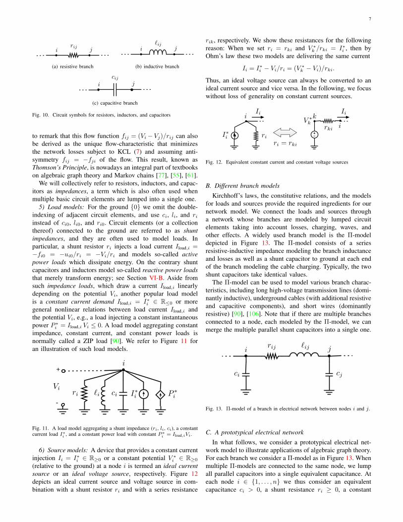
4) Constitutive relations: Here we consider three basiclinear circuit elements: resistors, inductors, and capacitors.These three elements are illustrated with their circuit symbolsin Figure 10. The voltage uij over a circuit element andcurrent flow fij through it satisfy the following well-knownconstitutive relations:• resistor: uij = rijfij , where rij > 0 is a resistance;• inductor: `ij d
dtfij = uij , where `ij > 0 is an inductance;• capacitor: cij d
dtuij = fij , where cij > 0 is a capacitance.The constitutive relation for a resistor, uij = rijfij known asOhm’s law gives together with KVL (9) the current flow overthe resistor as fij = uij/rij = (Vi − Vj)/rij . It is instructive
∗Our notation follows the convention that nodal (respectively, edge) vari-ables are denoted by capital (respectively, lower-case) letters.
7
i jrij
(a) resistive branch
i j`ij
(b) inductive branch
i jcij
(c) capacitive branch
Fig. 10. Circuit symbols for resistors, inductors, and capacitors
to remark that this flow function fij = (Vi−Vj)/rij can alsobe derived as the unique flow-characteristic that minimizesthe network losses subject to KCL (7) and assuming anti-symmetry fij = −fji of the flow. This result, known asThomson’s Principle, is nowadays an integral part of textbookson algebraic graph theory and Markov chains [77], [55], [61].
We will collectively refer to resistors, inductors, and capac-itors as impedances, a term which is also often used whenmultiple basic circuit elements are lumped into a single one.
5) Load models: For the ground {0} we omit the double-indexing of adjacent circuit elements, and use ci, li, and riinstead of ci0, li0, and ri0. Circuit elements (or a collectionthereof) connected to the ground are referred to as shuntimpedances, and they are often used to model loads. Inparticular, a shunt resistor ri injects a load current Iload,i =−fi0 = −ui0/ri = −Vi/ri and models so-called activepower loads which dissipate energy. On the contrary shuntcapacitors and inductors model so-called reactive power loadsthat merely transform energy; see Section VI-B. Aside fromsuch impedance loads, which draw a current Iload,i linearlydepending on the potential Vi, another popular load modelis a constant current demand Iload,i = I∗i ∈ R≤0 or moregeneral nonlinear relations between load current Iload,i andthe potential Vi, e.g., a load injecting a constant instantaneouspower P ∗i = Iload,i Vi ≤ 0. A load model aggregating constantimpedance, constant current, and constant power loads isnormally called a ZIP load [90]. We refer to Figure 11 foran illustration of such load models.
P ⇤i
i
I⇤iri `i ci
+
-
Vi
Fig. 11. A load model aggregating a shunt impedance (ri, li, ci), a constantcurrent load I∗i , and a constant power load with constant P ∗i = Iload,iVi.
6) Source models: A device that provides a constant currentinjection Ii = I∗i ∈ R≥0 or a constant potential V ∗i ∈ R≥0
(relative to the ground) at a node i is termed an ideal currentsource or an ideal voltage source, respectively. Figure 12depicts an ideal current source and voltage source in com-bination with a shunt resistor ri and with a series resistance
rik, respectively. We show these resistances for the followingreason: When we set ri = rki and V ∗k /rki = I∗i , then byOhm’s law these two models are delivering the same current
Ii = I∗i − Vi/ri = (V ∗k − Vi)/rki.Thus, an ideal voltage source can always be converted to anideal current source and vice versa. In the following, we focuswithout loss of generality on constant current sources.
i
riI⇤i
i=+
V ⇤k
rki
k
ri = rki
Ii Ii
Fig. 12. Equivalent constant current and constant voltage sources
B. Different branch models
Kirchhoff’s laws, the constitutive relations, and the modelsfor loads and sources provide the required ingredients for ournetwork model. We connect the loads and sources througha network whose branches are modeled by lumped circuitelements taking into account losses, charging, waves, andother effects. A widely used branch model is the Π-modeldepicted in Figure 13. The Π-model consists of a seriesresistive-inductive impedance modeling the branch inductanceand losses as well as a shunt capacitor to ground at each endof the branch modeling the cable charging. Typically, the twoshunt capacitors take identical values.
The Π-model can be used to model various branch charac-teristics, including long high-voltage transmission lines (domi-nantly inductive), underground cables (with additional resistiveand capacitive components), and short wires (dominantlyresistive) [90], [106]. Note that if there are multiple branchesconnected to a node, each modeled by the Π-model, we canmerge the multiple parallel shunt capacitors into a single one.
i jrij `ij
ci cj
Fig. 13. Π-model of a branch in electrical network between nodes i and j.
C. A prototypical electrical network
In what follows, we consider a prototypical electrical net-work model to illustrate applications of algebraic graph theory.For each branch we consider a Π-model as in Figure 13. Whenmultiple Π-models are connected to the same node, we lumpall parallel capacitors into a single equivalent capacitance. Ateach node i ∈ {1, . . . , n} we thus consider an equivalentcapacitance ci > 0, a shunt resistance ri ≥ 0, a constant
8
current injection I∗i ∈ R, and a constant power injectionP ∗i ∈ R modeling sources and loads as in Figures 11 and12. In this case, the network equations are
KCL: I = Bf , (10a)
KVL: u = BTV , (10b)
ground: I = Iload − CV , (10c)
branch: Lf = u−Rf , (10d)load: Iload = I∗ + P ∗ � V −GV , (10e)
where R,L,C,G are diagonal matrices of rij , `ij , ci, and thesymbol gi = 1/ri conventionally denotes the shunt conduc-tance (reciprocal of resistance). Finally, I∗ = (I∗1 , . . . , I
∗n) and
P ∗ are the vectors of constant current and power injections.It is convenient to reduce the network equations (10) to a
state-space model defined in terms of the variables V and fassociated with the capacitive and inductive storage elements.By inserting (10a), (10e) in (10c), respectively, (10b) in (10d),we obtain[C
L
] [V
f
]=
[−G −BBT −R
] [Vf
]+
[I∗ + P ∗ � V
0m
]. (11)
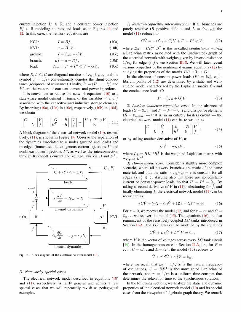
A block-diagram of the electrical network model (10), respec-tively, (11), is shown in Figure 14. Observe the separation ofthe dynamics associated to n nodes (ground and loads) andm edges (branches), the exogenous current injections I∗ andnonlinear power injections P ∗, as well as the interconnectionthrough Kirchhoff’s current and voltage laws via B and B>.
B BT
`ijdfij
dt= uij � rijfij
. . .
. . .
cidVi
dt= Iload � Ii
. . .
. . .
V
uf
_
ground dynamics
branch dynamics
I
KVLKCL
. . .
. . .I⇤i + P ⇤
i /Vi � giVi
loads
+Iload
I⇤i , P ⇤i
Fig. 14. Block-diagram of the electrical network model (10).
D. Noteworthy special cases
The electrical network model described in equations (10)and (11), respectively, is fairly general and admits a fewspecial cases that we will repeatedly revisit as pedagogicalexamples.
1) Resistive-capacitive interconnection: If all branches arepurely resistive (R positive definite and L = 0m×m), themodel (11) reduces to
CV = − (LR +G)V + I∗ + P ∗ � V , (12)
where LR = BR−1BT is the so-called conductance matrix,a Laplacian matrix associated with the (undirected) graph ofthe electrical network with weights given by inverse resistance1/rij for edge {i, j}; see Section III-8. We will later revealvarious properties of the nonlinear dynamic equations (12) bystudying the properties of the matrix BR−1BT +G.
In the absence of constant-power loads (P ∗ = 0n), equi-librium points of (12) are determined by a static and well-studied model characterized by the Laplacian matrix LR andthe conductance loads G:
I∗ = (LR +G)V . (13)
2) Lossless inductive-capacitive case: In the absence ofloads (G = 0n×n and I∗ = P ∗ = 0n) and dissipative elements(R = 0m×m) — that is, in an entirely lossless circuit — theelectrical network model (11) can be re-written as
[C
L
] [V
f
]=
[0 −BBT 0
] [Vf
], (14)
or by taking another derivative of V , as
CV = −LLV , (15)
where LL = BL−1BT is the weighted Laplacian matrix withweights L−1.
3) Homogeneous case: Consider a slightly more complexscenario, where all network branches are made of the samematerial, and thus the ratio of lij/rij = τ is constant for alledges {i, j} ∈ E . Assume also that there are no constant-current or constant-power loads, so that I∗ = P ∗ = 0n. Bytaking a second derivative of V in (11), substituting for f , andfinally eliminating f , the electrical network model (11) can bere-written as
τCV + (τG+ C)V + (LR +G)V = 0n . (16)
For τ = 0, we recover the model (12) and for τ =∞ and G =0n×n, we recover the model (15). The equations (16) are alsoreminiscent of the resistively coupled LC tanks introduced inSection II-A. The LC tanks can be modeled by the equations
CV + LRV + L−1V = 0n , (17)
where V is the vector of voltages across every LC tank circuit[49]. In the homogeneous case in Section II-A, i.e., for R =rIm, C = cIn, and L = `In, the model (17) reduces to
V + τ ′LV + ω20V = 0n ,
where we recall that ω0 = 1/√`c is the natural frequency
of oscillations, L = BBT is the unweighted Laplacian ofthe network, and τ ′ = 1/rc is a uniform time-constant thatdetermines the relaxation time to the synchronous solution.
In the following sections, we analyze the static and dynamicproperties of the electrical network model (10) and its specialcases from the viewpoint of algebraic graph theory. We remark
9
that most of the following approaches extend (either directlyor at least conceptually) to richer classes of electrical networkswith switching behavior as in power electronics [60], [162],multi-physical dynamics as in synchronous generators [63],[74], or nonlinear oscillators [152], [47], [39], among others.
V. STRUCTURE AND DYNAMICS OF LINEAR ELECTRICALNETWORKS
In what follows, we explain how the structure of an electri-cal network (in terms of its topology and impedances) revealsvarious insights about the associated electrical dynamics. Theinterplay of structure and dynamics is revealed through thealgebraic graph theory methods introduced in Section III.This section focuses on the case of linear electrical networks,described by special cases of the general model (11). The studyof nonlinear networks is deferred to Section VI.
A. Static resistive networks
We begin our analysis with the case of a static resistivenetwork with no constant power loads, as described by (13).For simplicity of notation, let us drop the super- and subscriptsin this section and simply rewrite (13) as
I = (L+G)V , (18)
where L = LT ∈ Rn×n is a symmetric and irreducibleLaplacian matrix, G ∈ Rn×n is a diagonal matrix withnonnegative diagonal entries, and I, V ∈ Rn are constantvectors. We remark that equation (18) is also of interestindependently of circuits, as linear diffusive equations withLaplacian matrices arise all throughout the sciences [138].
1) Characteristics of solutions and Laplacian inverses: Weexplore the solution space of the resistive circuit equation (18).We consider the singular and non-singular case separately.
Singular circuit equations: When G = 0n×n, we knowfrom Section III-6 that L is singular with Ker(L) = span(1n)and with Im(L) = 1⊥n . Hence, equation (18) admits a solutionif and only if I ∈ 1⊥n , that is, the current injections arebalanced: 1T
nI = 0. In this case, the solution is given by
V = Vhom + Vpart = α · 1n + L†I , (19)
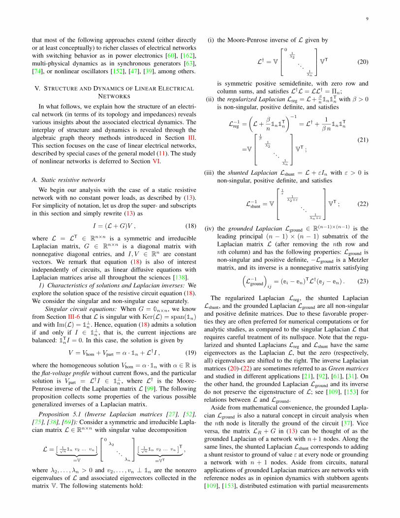
where the homogeneous solution Vhom = α ·1n with α ∈ R isthe flat-voltage profile without current flows, and the particularsolution is Vpart = L†I ∈ 1⊥n , where L† is the Moore-Penrose inverse of the Laplacian matrix L [99]. The followingproposition collects some properties of the various possiblegeneralized inverses of a Laplacian matrix.
Proposition 5.1 (Inverse Laplacian matrices [27], [52],[75], [38], [69]): Consider a symmetric and irreducible Lapla-cian matrix L ∈ Rn×n with singular value decomposition
L = [ 1√n
1n v2 ... vn ]︸ ︷︷ ︸=V
0λ2
. . .λn
[ 1√
n1n v2 ... vn ]
T
︸ ︷︷ ︸=VT
,
where λ2, . . . , λn > 0 and v2, . . . , vn ⊥ 1n are the nonzeroeigenvalues of L and associated eigenvectors collected in thematrix V. The following statements hold:
(i) the Moore-Penrose inverse of L given by
L† = V
01λ2
. . .1λn
VT (20)
is symmetric positive semidefinite, with zero row andcolumn sums, and satisfies L†L = LL† = Πn;
(ii) the regularized Laplacian Lreg = L+ βn1n1T
n with β > 0is non-singular, positive definite, and satisfies
L−1reg =
(L+
β
n1n1T
n
)−1
= L† +1
β n1n1T
n
=V
1β
1λ2
. . .1λn
VT ;
(21)
(iii) the shunted Laplacian Lshunt = L + εIn with ε > 0 isnon-singular, positive definite, and satisfies
L−1shunt = V
1ε
1λ2+ε
. . .1
λn+ε
VT ; (22)
(iv) the grounded Laplacian Lground ∈ R(n−1)×(n−1) is theleading principal (n − 1) × (n − 1) submatrix of theLaplacian matrix L (after removing the nth row andnth column) and has the following properties: Lground isnon-singular and positive definite, −Lground is a Metzlermatrix, and its inverse is a nonnegative matrix satisfying
(L−1
ground
)ij
= (ei − en)TL†(ej − en) . (23)
The regularized Laplacian Lreg, the shunted LaplacianLshunt, and the grounded Laplacian Lground are all non-singularand positive definite matrices. Due to these favorable proper-ties they are often preferred for numerical computations or foranalytic studies, as compared to the singular Laplacian L thatrequires careful treatment of its nullspace. Note that the regu-larized and shunted Laplacians Lreg and Lshunt have the sameeigenvectors as the Laplacian L, but the zero (respectively,all) eigenvalues are shifted to the right. The inverse Laplacianmatrices (20)-(22) are sometimes referred to as Green matricesand studied in different applications [21], [92], [61], [31]. Onthe other hand, the grounded Laplacian Lground and its inversedo not preserve the eigenstructure of L; see [109], [153] forrelations between L and Lground.
Aside from mathematical convenience, the grounded Lapla-cian Lground is also a natural concept in circuit analysis whenthe nth node is literally the ground of the circuit [37]. Viceversa, the matrix LR + G in (13) can be thought of as thegrounded Laplacian of a network with n+1 nodes. Along thesame lines, the shunted Laplacian Lshunt corresponds to addinga shunt resistor to ground of value ε at every node or groundinga network with n + 1 nodes. Aside from circuits, naturalapplications of grounded Laplacian matrices are networks withreference nodes as in opinion dynamics with stubborn agents[109], [153], distributed estimation with partial measurements
10
[10], or platooning of vehicles [76]. The grounded LaplacianLground is also an interesting algebraic graph and matrix theoryconcept in its own right and studied in [100], [69].
Non-singular circuit equations: In case that G has atleast one positive diagonal entry, then −(L+G) is a HurwitzMetzler matrix, as discussed in Section III-7 and Appendix A.The solution to (18) is therefore unique, and is given by
V = (L+G)−1I . (24)
The matrix L + G is sometimes called a loopy Laplacianmatrix since the non-zero diagonal entry represents a self-loopin the graph [52]. This matrix can also be thought of as thegrounded Laplacian matrix of an appropriate (n+1)×(n+1)-dimensional Laplacian matrix [52]. Since −(L+G) is Metzler,Hurwitz, and irreducible, then we know from Section III-7 that(L+G)−1 is a positive matrix. An important consequence isthat if the current injections I in (24) are nonnegative with atleast one strictly positive injection, then the unique voltagesolution V is a strictly positive vector; this is in contrastto the singular case (19). For example, this occurs if thecurrent injections I arise from converting voltage sources intocurrent sources (Section IV-A6). The matrices Lreg, Lground,Lshunt, and (L+G) are all positive definite, and their inversescan be further characterized in terms of their so-called decayproperties [46], [15], [100]. These decay properties reveal thatthe effect a current injection Ii at node i on the potential Vj ofanother node j diminishes according to the distance betweennodes i and j; we now explore this distance concept further.
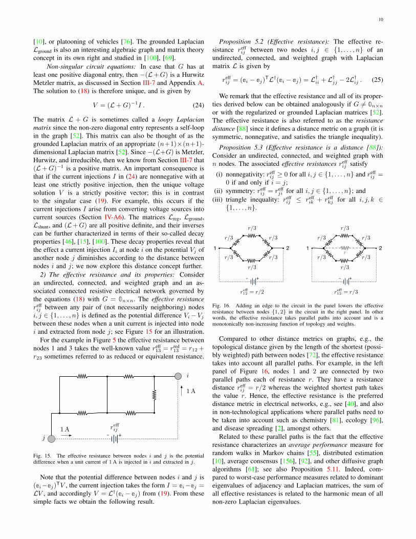
2) The effective resistance and its properties: Consideran undirected, connected, and weighted graph and an as-sociated connected resistive electrical network governed bythe equations (18) with G = 0n×n. The effective resistancereffij between any pair of (not necessarily neighboring) nodesi, j ∈ {1, . . . , n} is defined as the potential difference Vi−Vjbetween these nodes when a unit current is injected into nodei and extracted from node j; see Figure 15 for an illustration.
For the example in Figure 5 the effective resistance betweennodes 1 and 3 takes the well-known value reff
13 = rred13 = r12 +
r23 sometimes referred to as reduced or equivalent resistance.
+
i
j
re↵ij
1 A
1 A-
Fig. 15. The effective resistance between nodes i and j is the potentialdifference when a unit current of 1 A is injected in i and extracted in j.
Note that the potential difference between nodes i and j is(ei−ej)TV , the current injection takes the form I = ei−ej =LV , and accordingly V = L†(ei − ej) from (19). From thesesimple facts we obtain the following result.
Proposition 5.2 (Effective resistance): The effective re-sistance reff
ij between two nodes i, j ∈ {1, . . . , n} of anundirected, connected, and weighted graph with Laplacianmatrix L is given by
reffij = (ei − ej)
TL†(ei − ej) = L†ii + L†jj − 2L†ij . (25)
We remark that the effective resistance and all of its proper-ties derived below can be obtained analogously if G 6= 0n×nor with the regularized or grounded Laplacian matrices [52].The effective resistance is also referred to as the resistancedistance [88] since it defines a distance metric on a graph (it issymmetric, nonnegative, and satisfies the triangle inequality).
Proposition 5.3 (Effective resistance is a distance [88]):Consider an undirected, connected, and weighted graph withn nodes. The associated effective resistances reff
ij satisfy
(i) nonnegativity: reffij ≥ 0 for all i, j ∈ {1, . . . , n} and reff
ij =0 if and only if i = j;
(ii) symmetry: reffij = reff
ji for all i, j ∈ {1, . . . , n}; and(iii) triangle inequality: reff
ij ≤ reffik + reff
kj for all i, j, k ∈{1, . . . , n}.
r/3 r/3
r/3
r/3 r/3
r/3
1 2
+-
r/3 r/3
r/3
r/3 r/3
r/3
1 2
+
re↵12 = r/3
-
r
re↵12 = r/2
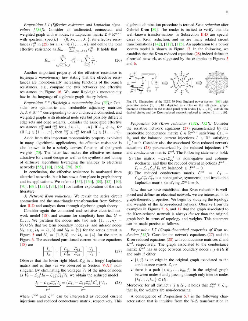
Fig. 16. Adding an edge to the circuit in the panel lowers the effectiveresistance between nodes {1, 2} in the circuit in the right panel. In otherwords, the effective resistance takes parallel paths into account and is amonotonically non-increasing function of topology and weights.
Compared to other distance metrics on graphs, e.g., thetopological distance given by the length of the shortest (possi-bly weighted) path between nodes [72], the effective resistancetakes into account all parallel paths. For example, in the leftpanel of Figure 16, nodes 1 and 2 are connected by twoparallel paths each of resistance r. They have a resistancedistance reff
ij = r/2 whereas the weighted shortest path takesthe value r. Hence, the effective resistance is the preferreddistance metric in electrical networks, e.g., see [40], and alsoin non-technological applications where parallel paths need tobe taken into account such as chemistry [81], ecology [96],and disease spreading [2], amongst others.
Related to these parallel paths is the fact that the effectiveresistance characterizes an average performance measure forrandom walks in Markov chains [55], distributed estimation[10], average consensus [156], [92], and other diffusive graphalgorithms [61]; see also Proposition 5.11. Indeed, com-pared to worst-case performance measures related to dominanteigenvalues of adjacency and Laplacian matrices, the sum ofall effective resistances is related to the harmonic mean of allnon-zero Laplacian eigenvalues.
11
Proposition 5.4 (Effective resistance and Laplacian eigen-values [154]): Consider an undirected, connected, andweighted graph with n nodes, its Laplacian matrix L ∈ Rn×nwith spectrum spec(L) = {0, λ2, . . . , λn}, its effective resis-tances reff
ij in (25) for all i, j ∈ {1, . . . , n}, and define the totaleffective resistance as Rtot =
∑ni,j=1,i<j r
effij . It holds that
Rtot =
n∑
i,j=1,i<j
reffij = n
n∑
i=2
1
λi. (26)
Another important property of the effective resistance isRayleigh’s monotonicity law stating that the effective resis-tances are monotonically increasing functions of the branchresistances, e.g., compare the two networks and effectiveresistances in Figure 16. We state Rayleigh’s monotonicitylaw in the language of algebraic graph theory below.
Proposition 5.5 (Rayleigh’s monotonicity law [55]): Con-sider two symmetric and irreducible adjacency matricesA, A ∈ Rn×n corresponding to two undirected, connected, andweighted graphs with identical node sets but possibly differentedge sets and edge weights. Consider the associated effectiveresistances reff
ij and reffij for i, j ∈ {1, . . . , n}. If Aij ≥ Aij for
all i, j ∈ {1, . . . , n}, then reffij ≤ reff
ij for all i, j ∈ {1, . . . , n}.Aside from this important monotonicity property exploited
in many algorithmic applications, the effective resistance isalso known to be a strictly convex function of the graphweights [70]. The latter fact makes the effective resistanceattractive for circuit design as well as the synthesis and tuningof diffusive algorithms leveraging the analogy to electricalnetworks [55], [10], [156], [70], [92].
In conclusion, the effective resistance is motivated fromelectrical networks, but it has now a firm place in graph theoryand its applications. We refer to [55], [154], [88], [52], [10],[70], [69], [157], [75], [61] for further exploration of the richliterature.
3) Network Kron reduction: We revisit the series circuitcontraction and the star-triangle transformation from Subsec-tion II-D and analyze them through algebraic graph theory.
Consider again the connected and resistive electrical net-work model (18), and assume for simplicity here that G =0n×n. We partition the nodes into two sets {1, . . . , n} =U1 ∪ U2 that we term boundary nodes U1 and interior nodesU2, e.g., U1 = {1, 3} and U2 = {2} for the series circuit inFigure 5 and U1 = {1, 2, 3} and U2 = {4} for the star inFigure 6. The associated partitioned current-balance equations(18) are [
I1I2
]=
[L11 L12
LT12 L22
] [V1
V2
]. (27)
Observe that the lower-right block L22 is a loopy Laplacianmatrix and is thus (as we observed in Section V-A1) non-singular. By eliminating the voltages V2 of the interior nodesas V2 = L−1
22 I2 − L−122 LT
12V1, we obtain the reduced model
I1 − L12L−122 I2︸ ︷︷ ︸
I red
=(L11 − L12L−1
22 LT12
)︸ ︷︷ ︸
Lred
V1 , (28)
where I red and Lred can be interpreted as reduced currentinjections and reduced conductance matrix, respectively. This
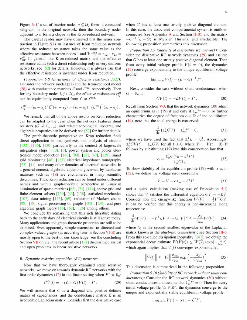
algebraic elimination procedure is termed Kron reduction afterGabriel Kron [89]. The reader is invited to verify that thewell-known transformations in Subsection II-D are specialcases of Kron reduction, and so are many related circuittransformations [142], [117], [115]. An application to a powersystem model is shown in Figure 17. In the following, weestablish that the Kron-reduced equations (28) indeed define anelectrical network, as suggested by the examples in Figures 5and 6.
2
10
30 25
8
37
29
9
38
23
7
36
22
635
19
4
3320
5
34
10
3
32
6
2
31
1
8
7
5
4
3
18
17
26
2728
24
21
16
1514
13
12
11
1
39
9
109
7
6
4
5
3
2
1
8
15
512
1110
7
8
9
4
3
1
2
17
18
14
16
19
20
21
24
26
27
28
31
32
34 33
36
38
39 22
35
6
13
30
37
25
29
23
1
10
8
2
3
6
9
4
7
5
F
Fig. 9. The New England test system [10], [11]. The system includes10 synchronous generators and 39 buses. Most of the buses have constantactive and reactive power loads. Coupled swing dynamics of 10 generatorsare studied in the case that a line-to-ground fault occurs at point F near bus16.
test system can be represented by
δi = ωi,Hi
πfsωi = −Diωi + Pmi − GiiE
2i −
10∑
j=1,j =i
EiEj ·
· {Gij cos(δi − δj) + Bij sin(δi − δj)},
⎫⎪⎪⎬⎪⎪⎭
(11)
where i = 2, . . . , 10. δi is the rotor angle of generator i withrespect to bus 1, and ωi the rotor speed deviation of generatori relative to system angular frequency (2πfs = 2π × 60Hz).δ1 is constant for the above assumption. The parametersfs, Hi, Pmi, Di, Ei, Gii, Gij , and Bij are in per unitsystem except for Hi and Di in second, and for fs in Helz.The mechanical input power Pmi to generator i and themagnitude Ei of internal voltage in generator i are assumedto be constant for transient stability studies [1], [2]. Hi isthe inertia constant of generator i, Di its damping coefficient,and they are constant. Gii is the internal conductance, andGij + jBij the transfer impedance between generators iand j; They are the parameters which change with networktopology changes. Note that electrical loads in the test systemare modeled as passive impedance [11].
B. Numerical Experiment
Coupled swing dynamics of 10 generators in thetest system are simulated. Ei and the initial condition(δi(0),ωi(0) = 0) for generator i are fixed through powerflow calculation. Hi is fixed at the original values in [11].Pmi and constant power loads are assumed to be 50% at theirratings [22]. The damping Di is 0.005 s for all generators.Gii, Gij , and Bij are also based on the original line datain [11] and the power flow calculation. It is assumed thatthe test system is in a steady operating condition at t = 0 s,that a line-to-ground fault occurs at point F near bus 16 att = 1 s−20/(60Hz), and that line 16–17 trips at t = 1 s. Thefault duration is 20 cycles of a 60-Hz sine wave. The faultis simulated by adding a small impedance (10−7j) betweenbus 16 and ground. Fig. 10 shows coupled swings of rotorangle δi in the test system. The figure indicates that all rotorangles start to grow coherently at about 8 s. The coherentgrowing is global instability.
C. Remarks
It was confirmed that the system (11) in the New Eng-land test system shows global instability. A few comments
0 2 4 6 8 10-5
0
5
10
15
δi /
ra
d
10
02
03
04
05
0 2 4 6 8 10-5
0
5
10
15
δi /
ra
d
TIME / s
06
07
08
09
Fig. 10. Coupled swing of phase angle δi in New England test system.The fault duration is 20 cycles of a 60-Hz sine wave. The result is obtainedby numerical integration of eqs. (11).
are provided to discuss whether the instability in Fig. 10occurs in the corresponding real power system. First, theclassical model with constant voltage behind impedance isused for first swing criterion of transient stability [1]. This isbecause second and multi swings may be affected by voltagefluctuations, damping effects, controllers such as AVR, PSS,and governor. Second, the fault durations, which we fixed at20 cycles, are normally less than 10 cycles. Last, the loadcondition used above is different from the original one in[11]. We cannot hence argue that global instability occurs inthe real system. Analysis, however, does show a possibilityof global instability in real power systems.
IV. TOWARDS A CONTROL FOR GLOBAL SWING
INSTABILITY
Global instability is related to the undesirable phenomenonthat should be avoided by control. We introduce a keymechanism for the control problem and discuss controlstrategies for preventing or avoiding the instability.
A. Internal Resonance as Another Mechanism
Inspired by [12], we here describe the global instabilitywith dynamical systems theory close to internal resonance[23], [24]. Consider collective dynamics in the system (5).For the system (5) with small parameters pm and b, the set{(δ,ω) ∈ S1 × R | ω = 0} of states in the phase plane iscalled resonant surface [23], and its neighborhood resonantband. The phase plane is decomposed into the two parts:resonant band and high-energy zone outside of it. Here theinitial conditions of local and mode disturbances in Sec. IIindeed exist inside the resonant band. The collective motionbefore the onset of coherent growing is trapped near theresonant band. On the other hand, after the coherent growing,it escapes from the resonant band as shown in Figs. 3(b),4(b), 5, and 8(b) and (c). The trapped motion is almostintegrable and is regarded as a captured state in resonance[23]. At a moment, the integrable motion may be interruptedby small kicks that happen during the resonant band. That is,the so-called release from resonance [23] happens, and thecollective motion crosses the homoclinic orbit in Figs. 3(b),4(b), 5, and 8(b) and (c), and hence it goes away fromthe resonant band. It is therefore said that global instability
!"#$%&'''%()(*%(+,-.,*%/012-3*%)0-4%5677*%899: !"#$%&'
(')$
Authorized licensed use limited to: Univ of Calif Santa Barbara. Downloaded on June 10, 2009 at 14:48 from IEEE Xplore. Restrictions apply.
Fig. 17. Illustration of the IEEE 39 New England power system [105] withgenerator nodes {1, . . . , 10} depicted as circles on the left panel; graph-theoretic abstraction in the middle panel with nodes {1, . . . , 10} outside thedashed circle; and the Kron-reduced network reduced to nodes {1, . . . , 10}.
Proposition 5.6 (Kron reduction [132], [52]): Considerthe resistive network equations (27) parameterized by theirreducible conductance matrix L ∈ Rn×n satisfying L1n =0n and the balanced current injections I ∈ Rn satisfying1TnI = 0. Consider also the associated Kron-reduced network
equations (28) parameterized by the reduced injections I red
and conductance matrix Lred. The following statements hold:(i) The matrix −L12L−1
22 is nonnegative and column-stochastic, and thus the reduced current injections I red =I1 − L12L−1
22 I2 are balanced: 1TI red = 0.(ii) The reduced conductance matrix Lred = L11 −L12L−1
22 LT12 is a nonnegative, symmetric, and irreducible
Laplacian matrix satisfying Lred1 = 0.
Now that we have established that Kron reduction is well-posed and defines an electrical network, we are interested in itsgraph-theoretic properties. We begin by studying the topologyand weights of the Kron-reduced network. Observe from theexamples in Figures 5, 6, and 17 that the graph associated tothe Kron-reduced network is always denser than the originalgraph both in terms of topology and weights. This statementcan be made precise as follows.
Proposition 5.7 (Graph-theoretical properties of Kron re-duction [52]): Consider the network equations (27) and theKron-reduced equations (28) with conductance matrices L andLred, respectively. The graph associated to the conductancematrix Lred has an edge between boundary nodes i, j ∈ U1 ifand only if either• {i, j} is an edge in the original graph associated to the
conductance matrix L, or• there is a path {i, k1, . . . , km, j} in the original graph
between nodes i and j passing through only interior nodes{k1, . . . , km} ⊂ U2.
Moreover, for all distinct i, j ∈ U1, it holds that Lredij ≤ Lij ,
that is, the weights are non-decreasing.
A consequence of Proposition 5.7 is the following char-acterization that is intuitive from the Y-∆ transformation in
12
Figure 6: if a set of interior nodes κ ⊆ U2 forms a connectedsubgraph in the original network, then the boundary nodesadjacent to κ form a clique in the Kron-reduced network.
The careful reader may have observed that the series con-traction in Figure 5 is an instance of Kron reduction networkwhere the reduced resistance takes the same value as theeffective resistance between nodes 1 and 3: rred
13 = r12 +r23 =reff13. In general, the Kron-reduced matrix and the effective
resistance admit such a direct relationship only in very uniformnetworks; see [52] for details. However, it is always true thatthe effective resistance is invariant under Kron reduction.
Proposition 5.8 (Invariance of effective resistance [52]):Consider the network model (27) and the Kron-reduced model(28) with conductance matrices L and Lred, respectively. Thenfor any boundary nodes i, j ∈ U1, the effective resistances reff
ij
can be equivalently computed from L or Lred:
reffij = (ei − ej)
TL†(ei − ej) = (ei − ej)T(Lred)† (ei − ej) .
We remark that all of the above results on Kron reductioncan be adapted to the case when the network features shuntresistors (G 6= 0n×n), and related topological, spectral, andalgebraic properties can be derived; see [52] for further details.
The graph-theoretic perspective on Kron reduction findsdirect application in the synthesis and analysis of circuits[132], [136], [150] particularly in the context of large-scaleintegration chips [113], [3], power system and power elec-tronics model reduction [143], [94], [28], [47], [129], smartgrid monitoring [48], [123], electrical impedance tomography[23], [41], and many other domains of electrical networks. Ina general context, algebraic equations governed by Laplacianmatrices such as (18) are encountered in many scientificdisciplines. Thus, Kron reduction can be found under differentnames and with a graph-theoretic perspective in Gaussianelimination of sparse matrices [65], [71], [114], sparse grid andfinite-element solvers [139], [43], [138], statistical mechanics[107], data mining [155], [69], reduction of Markov chains[98], [18], signal processing on graphs [108], [159], and purealgebraic graph theory [66], [62], [125] among others.
We conclude by remarking that this rich literature datingback to the early days of electrical circuits is still active today.Many applications and graph-theoretic properties are still to beexplored. Even apparently simple extensions to directed andcomplex-valued graphs (as occurring later in Section VI-B) aremostly open to the best of our knowledge; see the concludingSection VII or, e.g., the recent article [134] discussing classicaland open problems in linear resistive networks.
B. Dynamic resistive-capacitive (RC) networks
Now that we have thoroughly examined static resistivenetworks, we move on towards dynamic RC networks with thefirst-order dynamics (12) in the linear setting when P ∗ = 0n:
CV (t) = − (L+G)V (t) + I∗ . (29)
We will assume that C is a diagonal and positive definitematrix of capacitances, and the conductance matrix L is anirreducible Laplacian matrix. Consider first the dissipative case
when G has at least one strictly positive diagonal element.In this case, the associated compartmental system is outflow-connected (see Appendix A and Section II-B), and the matrix−C−1 (L+G) is Metzler, Hurwitz, and irreducible. Thefollowing proposition summarizes this discussion.
Proposition 5.9 (Stability of dissipative RC network): Con-sider the dissipative RC network dynamics (29) and assumethat G has at least one strictly positive diagonal element. Thenfrom every initial voltage profile V (t = 0), the dynamics(29) converge exponentially to the unique equilibrium voltageprofile
limt→∞ V (t) = (L+G)−1I∗ .
Next, consider the case without shunt conductances whenG = 0n×n:
CV (t) = −LV (t) + I∗ . (30)
Recall from Section V-A that the network dynamics (30) admitan equilibrium as in (19) if and only if 1T
nI∗ = 0. To further
characterize the degree of freedom α ∈ R of the equilibrium(19), note that the total charge is conserved:
d
dt
(1TnCV
)= 1T
nI∗ = 0 , (31)
where we have used the fact that 1TnL = 0T
n. Accordingly,1TnCV (t) = 1T
nCV0 for all t ≥ 0, where V0 = V (t = 0). Itfollows by substituting (19) into this conservation law that
α =1TnC(V0 − L†I∗)
1TnC1n
. (32)
To show stability of the equilibrium profile (19) with α as in(32), we define the voltage error coordinate
V = V − α1n − L†I∗ , (33)
and a quick calculation (making use of Proposition 5.1)shows that V satisfies the differential equation C ˙V = −LV .Consider now the energy-like function W (V ) = 1
2 VTCV .
It can be verified that this energy is non-increasing alongtrajectories:
d
dtW (V ) = −V TLV ≤ −λ2‖V ‖2 ≤ −
λ2
cmaxW (V ) , (34)
where λ2 is the second-smallest eigenvalue of the Laplacianmatrix known as the algebraic connectivity; see Section III-6.From this so-called dissipation inequality [147], we obtain theexponential decay estimate W (V (t)) ≤ W (V0) exp(− λ2
cmaxt),
which again implies that V (t) converges exponentially:∥∥∥V (t)
∥∥∥ ≤∥∥∥V0
∥∥∥ cmax
cminexp
(− λ2
2cmaxt
). (35)
This discussion is summarized in the following proposition.
Proposition 5.10 (Stability of RC network without shunt con-ductances): Consider the RC network dynamics (30) withoutshunt conductances and assume that 1T
nI∗ = 0. Then for every
initial voltage profile V0 ∈ Rn, the dynamics converge to theunique and exponentially stable equilibrium voltage profile
limt→∞ V (t) = α1n − L†I∗,
13
where α is given by (32). The convergence is exponential witha decay rate proportional to λ2 as in (35). Moreover, the totalcharge is conserved along solutions as in (31).
The following remarks are in order. In the absence ofexternal injections, I∗ = 0n, the voltages equalize to the flatprofile 1T
nCV0
1TnC1n
1n; this constant uniform voltage is a weightedaverage of the initial voltage values, with weights dependingon the capacitances. The features of the particular solutionL†I∗ have been discussed in detail in Section V-A. The voltageerror coordinate (33) is related to the disagreement vectorstudied in consensus problems [103], [33]. The exponentialdecay estimate λ2/cmax in (35) depends on the maximumcapacitance as well as on the algebraic connectivity λ2 ofthe network. The algebraic connectivity is a well-studiedquantity in algebraic graph theory dating back to the seminalwork by Fiedler [64]. For example, λ2 is a popular metricin graph partitioning and community detection [111], [67]as it quantifies the smallest bottleneck in the graph, where“smallest” is understood in our context as the minimal currentflow over any cut separating the nodes of an electrical network.
The exponential decay estimate (35) is achieved for a worst-case initial condition V0 aligned with the eigenvector v2 asso-ciated to the eigenvalue λ2. However, often one is interestedin an average integral-quadratic performance criterion
E[∫ ∞
0
V (t)TΠnV (t) dt
], (36)
where the expectation is with respect to a random initialerror voltage profile V0 with zero mean and E
[V0V
T0
]= Πn
(possibly due to a random realization of the current demandsI or initial voltages V0). The projector matrix Πn inducesthe global voltage error V TΠnV = ‖V − average(V )1n‖2,and discards values of V (t) and V0 aligned with 1n thatdo not affect the transient dynamics. The integral quadraticperformance metric criterion (36) is well-known in control andsignal processing under the name of an H2-norm of a system[161], and it is well-studied for the system (30) in the contextof consensus systems [29], [7], [156], power systems [126],[110], and random walks [55], [69], among others. In our caseand for identical capacitors C = In, the average performancecriterion (36) evaluates to an average of the inverse non-zeroLaplacian eigenvalues as in the total effective resistance (26).
Proposition 5.11 (Average performance of RC network[27]): Consider the RC network dynamics (30) with identicalcapacitors C = In, the voltage error coordinate (33), andthe average integral quadratic performance criterion (36) fora random initial condition V0 ∈ Rn with zero mean andE[V0V
T0
]= Πn. The performance criterion (36) evaluates to
E[∫ ∞
0
V (t)TΠnV (t) dt
]=
n∑
i=2
1
λi= Rtot/n , (37)
where Rtot is the total effective resistance (26).There are several equivalent interpretations of the H2-norm
(36) aside from characterizing the average convergence rate(37) [161]. For example, an equivalent interpretation is thesteady-state voltage variance when subjecting each node tonoisy current inputs or the transient energy dissipated by the
circuit after being subjected to impulsive current inputs arising,e.g., from line faults [38], [126]. While admittedly, the averageperformance index (36) is of minor importance to circuits,it plays a key role in the design of distributed algorithmswith diffusive dynamics [29], [7], [156], [55], [69], [92],[61], where the analogy to the effective resistance providesimportant intuition, and well-known concepts on the electricalside (such as Rayleigh’s monotonicity law) inspire and informthe design and analysis of algorithms. Finally, we remark thatthe above result can be extended to more general cost functionsthan (36), higher-order dynamics, and discrete-time settings[29], [7], [156], [110], [38], [130], [38], [130]. Extensions tononlinear circuits remain an open problem.
C. Dynamic resistive-inductive-capacitive (RLC) networks
In this section we analyze the full RLC network model (11)from Section IV-C, repeated here for convenience:[C
L
] [V
f
]=
[−G −BBT −R
] [Vf
]+
[I∗ + P ∗ � V
0m
].
Our approach will be to leverage the algebraic graph theorymethods introduced in Section III. We begin by highlightingthe energy conservation and dissipation properties of thenetwork system (11). Consider the electric and the magneticenergy associated to the network storage elements:
H(V, f) =1
2V TCV +
1
2fTLf . (38)
The time derivative of the energy (38) along trajectories of thenetwork dynamics (11) is given by the power balance
H(V, f) =
[Vf
]T [ −BBT
] [Vf
]
︸ ︷︷ ︸=0 (lossless power circulations)
−[Vf
]T [G
R
] [Vf
]
︸ ︷︷ ︸≤0 (power losses)
+V TI∗ + 1TnP∗
︸ ︷︷ ︸(external power supplied)
, (39)
where we used the identity V T(P ∗ � V ) = 1TnP∗. The last
term in the power balance equation (39) corresponds to theexternal power supplied to the network through the externalcurrent and power injections, the central term corresponds todissipation induced by shunt and branch resistances, and thefirst term evaluates to zero due to skew-symmetry of matrix inthe quadratic form. To further understand the role of the firstterm, consider the network (14) without branch dissipationR = 0 and without loads (G = 0, I∗ = P ∗ = 0n). In thiscase, the total energy is preserved H(V, f) = 0, and thusH(V (t), f(t)) = H(V0, f0) for all t ≥ 0, which says theellipsoidal level sets of the energy function (38) are invariant.In particular, since the system (14) is linear, these level sets arethe images of oscillating harmonic trajectories (V (t), f(t)).Thus, the dynamic behavior of the lossless network (14) andthe first term in the general power balance (39) correspond tolossless energy exchange (i.e., power circulations) between theinductive and capacitive storage elements. For identical timeconstants C = In, the dynamics (14) reduce to the Laplacianoscillator (15) and the solutions can be further characterized.
14
Proposition 5.12 (Circulations in lossless circuit [49]):Consider the lossless network model (14). The solution is asuperposition of n undamped harmonic signals. Moreover, ifC = In, then the frequencies† of these harmonic signals are√λi, i ∈ {1, . . . , n}, where λi are the eigenvalues of the L−1-
weighted Laplacian matrix LL = BL−1BT.
The power balance equation (39) is a special case of a so-called dissipation (in)equality (more specifically a passivityinequality) [147], [131], and the insights gained from it lay thefoundations for further analysis of general nonlinear electricalnetworks [95], [128] and other interconnected systems [133],[135], [104]. For example, another key insight is that, forpositive definite matrices G and R, the right-hand side of (39)is strictly negative for sufficiently large values of voltages Vand currents f . It follows that in this case, the trajectoriesof the nonlinear network dynamics (11) are always bounded.Notice also that the analysis of linear RC circuits, treatedpreviously in Subsection V-B, can be equivalently performedbased on matrix theory or dissipation inequalities such as (34).
We will defer a further nonlinear analysis to Section VI-Aand focus now on the linear and homogeneous case whenP ∗ = I∗ = 0n to showcase the tools of algebraic graph theoryfrom Section III. Consider the network dynamics
[C
L
] [V
f
]=
[−G −BBT −R
]
︸ ︷︷ ︸=A
[Vf
]. (40)
The network matrix A is related to so-called saddle or KKTmatrices [14] in quadratic optimization programs with linearequality constraints (where R = 0). We collect some proper-ties in the following proposition that is proved in Appendix B.
Proposition 5.13 (Spectrum of saddle matrices): Considerthe network matrix A in (40), where G and R are positivesemidefinite, and the graph associated to the incidence matrixB is connected. The matrix A has the following properties:
1) all eigenvalues are in the closed left half-plane:spec(A)⊂{λ ∈ C | <(λ) ≤ 0}. Moreover, all eigenvalueson the imaginary axis have equal algebraic and geometricmultiplicities;
2) if G and R are zero matrices, then all eigenvaluesof A are on the imaginary axis and spec(A) ={0, 0,±iλ2, . . . ,±iλn}, where {λ2, . . . , λn} are the non-zero eigenvalues of the unweighted Laplacian BBT;
3) if G and R are positive definite, then A is Hurwitz;4) if Ker(G) ∩ Im(B) = {0n}, then A has no eigenvalues
on the imaginary axis except for 0. Moreover, if G ispositive definite and B has full rank (i.e., the graph isacyclic), then A is Hurwitz; and
5) if Ker(R)∩ Im(BT) = {0n}, then A has no eigenvalueson the imaginary axis except for 0. Moreover, if R ispositive definite and Gii > 0 for at least one elementi ∈ {1, . . . , n}, then A is Hurwitz.
The above matrix spectrum results for A translate quicklyinto dynamic stability results for the system (40), since the
†Note that the 1st mode λ1 = 0 corresponding to average(V (t)) resultsin constant (0-frequency) average voltage since d
dtaverage(V (t)) = 0.
inductances and capacitances L and C do not change the sta-bility of A (which can be seen, e.g., by changing coordinatesto[C
12V L
12 f]). Property 1) guarantees that the dynamics
(40) are always marginally stable, possibly with sustainedoscillations or constant non-decaying modes. Whenever G(respectively, R) is positive definite, then property 4) (respec-tively, property 5)) guarantees that no sustained oscillationscan occur. However, in this case it is not true that all signalswill necessarily settle to zero. For example, assume that thatG is positive definite and R = 0; this satisfies the assumptionsof property 4). Then a possible equilibrium for (40) is
V ∗ = 0n , f∗ ∈ Ker(B) ,
that is, the equilibrium current flows f∗ live in the cycle spaceKer(B) of the graph; see Section III-9. Hence, any initialcurrent circulation f0 ∈ Ker(B) is persistent and does notdissipate. Of course, this is ruled out if either B has full rank(i.e., the graph is acyclic) or R is positive definite so thatdissipation forces all circulating flows vanish. Similarly, inthe scenario of property 5) with G = 0n×n and R positivedefinite, we observe that a possible equilibrium is
V ∗ ∈ Ker(BT) = span(1n) , f∗ = 0m ,
which allows for any uniform potential vector V ∗ analogousto the conservation of charge in (33). If at least one shuntresistance Gii > 0 is present, then dissipation forces V ∗ = 0n.
Several of the special cases we have considered thus farallow for a more detailed analysis of the linear networkdynamics (40). In particular, recall the Laplacian oscillatordynamics (15) analyzed in Proposition 5.12, the homogeneousnetwork dynamics (16), and the coupled `c-tanks (17) inFigure 2. These dynamics are all instances of the more generalsecond-order Laplacian flow
V + (kdIn + γdL)V + (kpIn + γpL)V = 0n, (41)
which can be written in state-space form as
d
dt
[V
V
]=
[0n×n In
−kpIn − γpL −kdIn − γdL
]
︸ ︷︷ ︸=Q
[V
V
], (42)
where L ∈ Rn×n is an irreducible and symmetric Laplacianmatrix, and kd, kp, γd, and γp are scalar and nonnegative gainsthat (if positive) induce a diffusive coupling or a resistivedissipation on the voltages V and their drifts V , respectively.
The dynamics (42) can be elegantly analyzed via a changeof coordinates V → VV , where V = [ 1√
n1n v2 ... vn ]
collects the eigenvectors of the Laplacian matrix L as inProposition 5.1. In these coordinates and after permuting theentries appropriately, the matrix Q governing the second-orderLaplacian flow (42) is similar to a block-diagonal matrix withn blocks, each of the form
[0 1
−kp − γpλi −kd − γdλi
], i ∈ {1, . . . , n} ,
where 0 = λ1 < λ2 ≤ · · · ≤ λn are the eigenvalues of theLaplacian matrix L. We can draw the following conclusions.
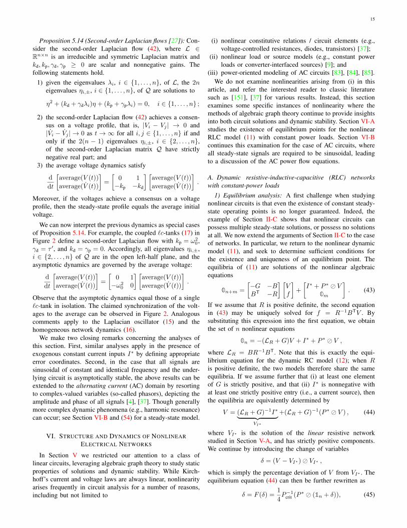
15
Proposition 5.14 (Second-order Laplacian flows [27]): Con-sider the second-order Laplacian flow (42), where L ∈Rn×n is an irreducible and symmetric Laplacian matrix andkd, kp, γd, γp ≥ 0 are scalar and nonnegative gains. Thefollowing statements hold.
1) given the eigenvalues λi, i ∈ {1, . . . , n}, of L, the 2neigenvalues ηi,±, i ∈ {1, . . . , n}, of Q are solutions to
η2 + (kd + γdλi)η + (kp + γpλi) = 0, i ∈ {1, . . . , n} ;
2) the second-order Laplacian flow (42) achieves a consen-sus on a voltage profile, that is, |Vi − Vj | → 0 and|Vi − Vj | → 0 as t→∞ for all i, j ∈ {1, . . . , n} if andonly if the 2(n − 1) eigenvalues ηi,±, i ∈ {2, . . . , n},of the second-order Laplacian matrix Q have strictlynegative real part; and
3) the average voltage dynamics satisfy
d
dt
[average(V (t))
average(V (t))
]=
[0 1−kp −kd
] [average(V (t))
average(V (t))
].
Moreover, if the voltages achieve a consensus on a voltageprofile, then the steady-state profile equals the average initialvoltage.
We can now interpret the previous dynamics as special casesof Proposition 5.14. For example, the coupled `c-tanks (17) inFigure 2 define a second-order Laplacian flow with kp = ω2
0 ,γd = τ ′, and kd = γp = 0. Accordingly, all eigenvalues ηi,±,i ∈ {2, . . . , n} of Q are in the open left-half plane, and theasymptotic dynamics are governed by the average voltage:
d
dt
[average(V (t))
average(V (t))
]=
[0 1−ω2
0 0
] [average(V (t))
average(V (t))
].
Observe that the asymptotic dynamics equal those of a single`c-tank in isolation. The claimed synchronization of the volt-ages to the average can be observed in Figure 2. Analogouscomments apply to the Laplacian oscillator (15) and thehomogeneous network dynamics (16).
We make two closing remarks concerning the analyses ofthis section. First, similar analyses apply in the presence ofexogenous constant current inputs I∗ by defining appropriateerror coordinates. Second, in the case that all signals aresinusoidal of constant and identical frequency and the under-lying circuit is asymptotically stable, the above results can beextended to the alternating current (AC) domain by resortingto complex-valued variables (so-called phasors), depicting theamplitude and phase of all signals [4], [37]. Though generallymore complex dynamic phenomena (e.g., harmonic resonance)can occur; see Section VI-B and (54) for a steady-state model.
VI. STRUCTURE AND DYNAMICS OF NONLINEARELECTRICAL NETWORKS
In Section V we restricted our attention to a class oflinear circuits, leveraging algebraic graph theory to study staticproperties of solutions and dynamic stability. While Kirch-hoff’s current and voltage laws are always linear, nonlinearityarises frequently in circuit analysis for a number of reasons,including but not limited to
(i) nonlinear constitutive relations / circuit elements (e.g.,voltage-controlled resistances, diodes, transistors) [37];
(ii) nonlinear load or source models (e.g., constant powerloads or converter-interfaced sources) [9]; and
(iii) power-oriented modeling of AC circuits [83], [84], [85].We do not examine nonlinearities arising from (i) in this
article, and refer the interested reader to classic literaturesuch as [151], [37] for various results. Instead, this sectionexamines some specific instances of nonlinearity where themethods of algebraic graph theory continue to provide insightsinto both circuit solutions and dynamic stability. Section VI-Astudies the existence of equilibrium points for the nonlinearRLC model (11) with constant power loads. Section VI-Bcontinues this examination for the case of AC circuits, whereall steady-state signals are required to be sinusoidal, leadingto a discussion of the AC power flow equations.
A. Dynamic resistive-inductive-capacitive (RLC) networkswith constant-power loads
1) Equilibrium analysis: A first challenge when studyingnonlinear circuits is that even the existence of constant steady-state operating points is no longer guaranteed. Indeed, theexample of Section II-C shows that nonlinear circuits canpossess multiple steady-state solutions, or possess no solutionsat all. We now extend the arguments of Section II-C to the caseof networks. In particular, we return to the nonlinear dynamicmodel (11), and seek to determine sufficient conditions forthe existence and uniqueness of an equilibrium point. Theequilibria of (11) are solutions of the nonlinear algebraicequations
0n+m =
[−G −BBT −R
] [Vf
]+
[I∗ + P ∗ � V
0m
]. (43)
If we assume that R is positive definite, the second equationin (43) may be uniquely solved for f = R−1BTV . Bysubstituting this expression into the first equation, we obtainthe set of n nonlinear equations
0n = −(LR +G)V + I∗ + P ∗ � V ,where LR = BR−1BT. Note that this is exactly the equi-librium equation for the dynamic RC model (12); when Ris positive definite, the two models therefore share the sameequilibria. If we assume further that (i) at least one elementof G is strictly positive, and that (ii) I∗ is nonnegative withat least one strictly positive entry (i.e., a current source), thenthe equilibria are equivalently determined by
V = (LR +G)−1I∗︸ ︷︷ ︸VI∗
+(LR +G)−1(P ∗ � V ) , (44)
where VI∗ is the solution of the linear resistive networkstudied in Section V-A, and has strictly positive components.We continue by introducing the change of variables
δ = (V − VI∗)� VI∗ ,which is simply the percentage deviation of V from VI∗ . Theequilibrium equation (44) can then be further rewritten as
δ = F (δ) =1
4P−1
crit (P ∗ � (1n + δ)), (45)
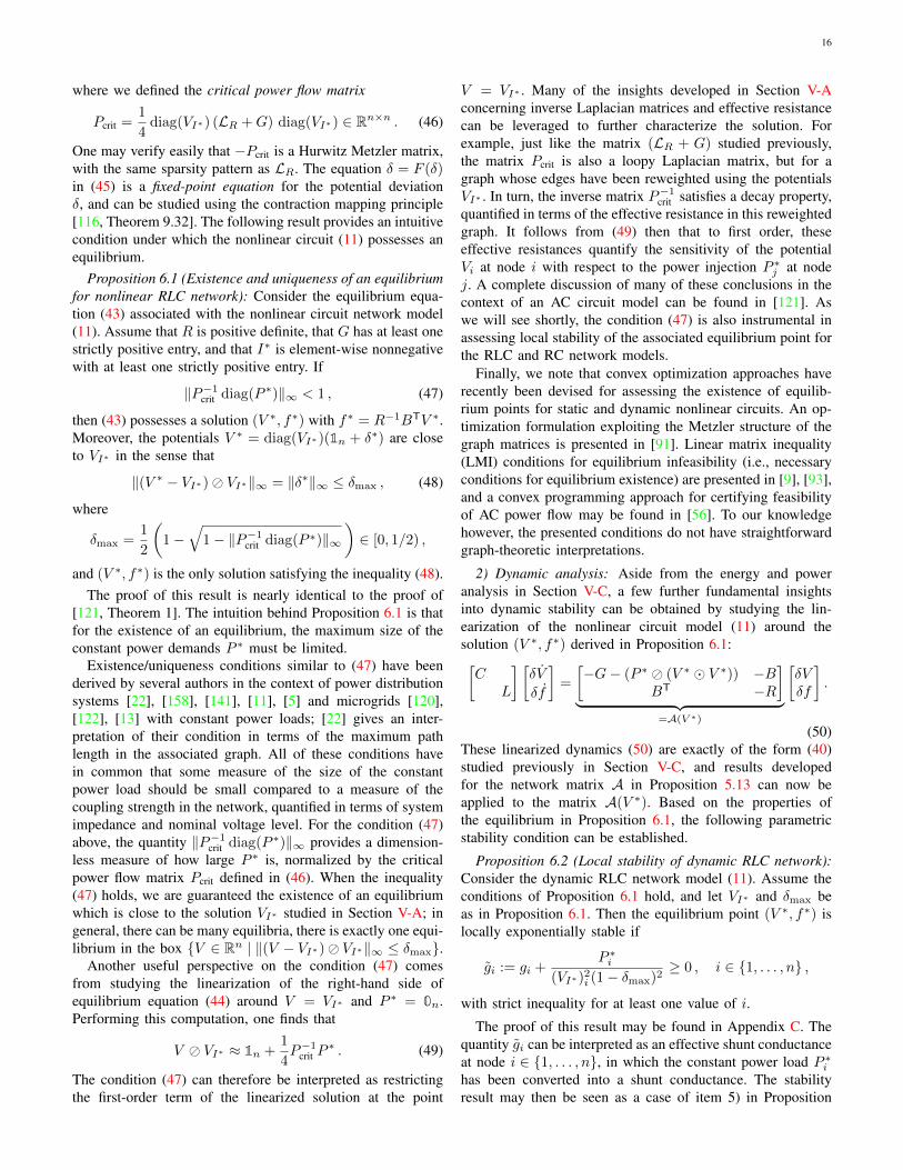
16
where we defined the critical power flow matrix
Pcrit =1
4diag(VI∗) (LR +G) diag(VI∗) ∈ Rn×n . (46)
One may verify easily that −Pcrit is a Hurwitz Metzler matrix,with the same sparsity pattern as LR. The equation δ = F (δ)in (45) is a fixed-point equation for the potential deviationδ, and can be studied using the contraction mapping principle[116, Theorem 9.32]. The following result provides an intuitivecondition under which the nonlinear circuit (11) possesses anequilibrium.
Proposition 6.1 (Existence and uniqueness of an equilibriumfor nonlinear RLC network): Consider the equilibrium equa-tion (43) associated with the nonlinear circuit network model(11). Assume that R is positive definite, that G has at least onestrictly positive entry, and that I∗ is element-wise nonnegativewith at least one strictly positive entry. If
‖P−1crit diag(P ∗)‖∞ < 1 , (47)
then (43) possesses a solution (V ∗, f∗) with f∗ = R−1BTV ∗.Moreover, the potentials V ∗ = diag(VI∗)(1n + δ∗) are closeto VI∗ in the sense that
‖(V ∗ − VI∗)� VI∗‖∞ = ‖δ∗‖∞ ≤ δmax , (48)
where
δmax =1
2
(1−
√1− ‖P−1
crit diag(P ∗)‖∞)∈ [0, 1/2) ,
and (V ∗, f∗) is the only solution satisfying the inequality (48).The proof of this result is nearly identical to the proof of
[121, Theorem 1]. The intuition behind Proposition 6.1 is thatfor the existence of an equilibrium, the maximum size of theconstant power demands P ∗ must be limited.
Existence/uniqueness conditions similar to (47) have beenderived by several authors in the context of power distributionsystems [22], [158], [141], [11], [5] and microgrids [120],[122], [13] with constant power loads; [22] gives an inter-pretation of their condition in terms of the maximum pathlength in the associated graph. All of these conditions havein common that some measure of the size of the constantpower load should be small compared to a measure of thecoupling strength in the network, quantified in terms of systemimpedance and nominal voltage level. For the condition (47)above, the quantity ‖P−1
crit diag(P ∗)‖∞ provides a dimension-less measure of how large P ∗ is, normalized by the criticalpower flow matrix Pcrit defined in (46). When the inequality(47) holds, we are guaranteed the existence of an equilibriumwhich is close to the solution VI∗ studied in Section V-A; ingeneral, there can be many equilibria, there is exactly one equi-librium in the box {V ∈ Rn | ‖(V − VI∗)� VI∗‖∞ ≤ δmax}.
Another useful perspective on the condition (47) comesfrom studying the linearization of the right-hand side ofequilibrium equation (44) around V = VI∗ and P ∗ = 0n.Performing this computation, one finds that
V � VI∗ ≈ 1n +1
4P−1
crit P∗ . (49)
The condition (47) can therefore be interpreted as restrictingthe first-order term of the linearized solution at the point
V = VI∗ . Many of the insights developed in Section V-Aconcerning inverse Laplacian matrices and effective resistancecan be leveraged to further characterize the solution. Forexample, just like the matrix (LR + G) studied previously,the matrix Pcrit is also a loopy Laplacian matrix, but for agraph whose edges have been reweighted using the potentialsVI∗ . In turn, the inverse matrix P−1
crit satisfies a decay property,quantified in terms of the effective resistance in this reweightedgraph. It follows from (49) then that to first order, theseeffective resistances quantify the sensitivity of the potentialVi at node i with respect to the power injection P ∗j at nodej. A complete discussion of many of these conclusions in thecontext of an AC circuit model can be found in [121]. Aswe will see shortly, the condition (47) is also instrumental inassessing local stability of the associated equilibrium point forthe RLC and RC network models.
Finally, we note that convex optimization approaches haverecently been devised for assessing the existence of equilib-rium points for static and dynamic nonlinear circuits. An op-timization formulation exploiting the Metzler structure of thegraph matrices is presented in [91]. Linear matrix inequality(LMI) conditions for equilibrium infeasibility (i.e., necessaryconditions for equilibrium existence) are presented in [9], [93],and a convex programming approach for certifying feasibilityof AC power flow may be found in [56]. To our knowledgehowever, the presented conditions do not have straightforwardgraph-theoretic interpretations.
2) Dynamic analysis: Aside from the energy and poweranalysis in Section V-C, a few further fundamental insightsinto dynamic stability can be obtained by studying the lin-earization of the nonlinear circuit model (11) around thesolution (V ∗, f∗) derived in Proposition 6.1:[C
L
] [δV
δf
]=
[−G− (P ∗ � (V ∗ � V ∗)) −B
BT −R
]
︸ ︷︷ ︸=A(V ∗)
[δVδf
].
(50)These linearized dynamics (50) are exactly of the form (40)studied previously in Section V-C, and results developedfor the network matrix A in Proposition 5.13 can now beapplied to the matrix A(V ∗). Based on the properties ofthe equilibrium in Proposition 6.1, the following parametricstability condition can be established.
Proposition 6.2 (Local stability of dynamic RLC network):Consider the dynamic RLC network model (11). Assume theconditions of Proposition 6.1 hold, and let VI∗ and δmax beas in Proposition 6.1. Then the equilibrium point (V ∗, f∗) islocally exponentially stable if
gi := gi +P ∗i
(VI∗)2i (1− δmax)2
≥ 0 , i ∈ {1, . . . , n} ,
with strict inequality for at least one value of i.
The proof of this result may be found in Appendix C. Thequantity gi can be interpreted as an effective shunt conductanceat node i ∈ {1, . . . , n}, in which the constant power load P ∗ihas been converted into a shunt conductance. The stabilityresult may then be seen as a case of item 5) in Proposition
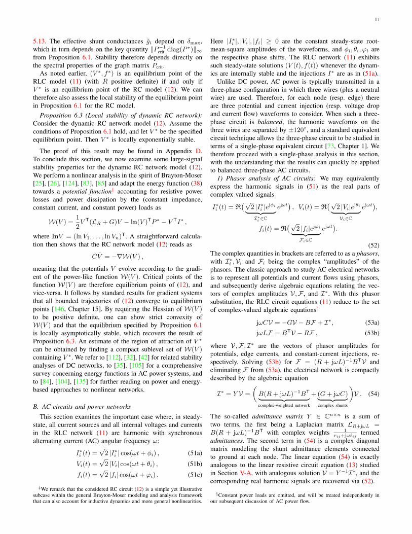
17
5.13. The effective shunt conductances gi depend on δmax,which in turn depends on the key quantity ‖P−1
crit diag(P ∗)‖∞from Proposition 6.1. Stability therefore depends directly onthe spectral properties of the graph matrix Pcrit.
As noted earlier, (V ∗, f∗) is an equilibrium point of theRLC model (11) (with R positive definite) if and only ifV ∗ is an equilibrium point of the RC model (12). We cantherefore also assess the local stability of the equilibrium pointin Proposition 6.1 for the RC model.
Proposition 6.3 (Local stability of dynamic RC network):Consider the dynamic RC network model (12). Assume theconditions of Proposition 6.1 hold, and let V ∗ be the specifiedequilibrium point. Then V ∗ is locally exponentially stable.
The proof of this result may be found in Appendix D.To conclude this section, we now examine some large-signalstability properties for the dynamic RC network model (12).We perform a nonlinear analysis in the spirit of Brayton-Moser[25], [26], [124], [83], [85] and adapt the energy function (38)towards a potential function‡ accounting for resistive powerlosses and power dissipation by the (constant impedance,constant current, and constant power) loads as
W(V ) =1
2V T(LR +G)V − ln(V )TP ∗ − V TI∗ ,
where lnV = (lnV1, . . . , lnVn)T. A straightforward calcula-tion then shows that the RC network model (12) reads as
CV = −∇W(V ) ,
meaning that the potentials V evolve according to the gradi-ent of the power-like function W(V ). Critical points of thefunction W(V ) are therefore equilibrium points of (12), andvice-versa. It follows by standard results for gradient systemsthat all bounded trajectories of (12) converge to equilibriumpoints [146, Chapter 15]. By requiring the Hessian of W(V )to be positive definite, one can show strict convexity ofW(V ) and that the equilibrium specified by Proposition 6.1is locally asymptotically stable, which recovers the result ofProposition 6.3. An estimate of the region of attraction of V ∗
can be obtained by finding a compact sublevel set of W(V )containing V ∗. We refer to [112], [32], [42] for related stabilityanalyses of DC networks, to [35], [105] for a comprehensivesurvey concerning energy functions in AC power systems, andto [84], [104], [135] for further reading on power and energy-based approaches to nonlinear networks.
B. AC circuits and power networks
This section examines the important case where, in steady-state, all current sources and all internal voltages and currentsin the RLC network (11) are harmonic with synchronousalternating current (AC) angular frequency ω:
I∗i (t) =√
2 |I∗i | cos(ωt+ φi) , (51a)
Vi(t) =√
2 |Vi| cos(ωt+ θi) , (51b)
fi(t) =√
2 |fi| cos(ωt+ ϕi) . (51c)
‡We remark that the considered RC circuit (12) is a simple yet illustrativesubcase within the general Brayton-Moser modeling and analysis frameworkthat can also account for inductive dynamics and more general nonlinearities.
Here |I∗i |, |Vi|, |fi| ≥ 0 are the constant steady-state root-mean-square amplitudes of the waveforms, and φi, θi, ϕi arethe respective phase shifts. The RLC network (11) exhibitssuch steady-state solutions (V (t), f(t)) whenever the dynam-ics are internally stable and the injections I∗ are as in (51a).
Unlike DC power, AC power is typically transmitted in athree-phase configuration in which three wires (plus a neutralwire) are used. Therefore, for each node (resp. edge) thereare three potential and current injection (resp. voltage dropand current flow) waveforms to consider. When such a three-phase circuit is balanced, the harmonic waveforms on thethree wires are separated by ±120◦, and a standard equivalentcircuit technique allows the three-phase circuit to be studied interms of a single-phase equivalent circuit [73, Chapter 1]. Wetherefore proceed with a single-phase analysis in this section,with the understanding that the results can quickly be appliedto balanced three-phase AC circuits.
1) Phasor analysis of AC circuits: We may equivalentlyexpress the harmonic signals in (51) as the real parts ofcomplex-valued signals
I∗i (t) = R(√
2 |I∗i |ejφi
︸ ︷︷ ︸I∗i ∈C
ejωt), Vi(t) = R
(√2 |Vi|ejθi
︸ ︷︷ ︸Vi∈C
ejωt),
fi(t) = R(√
2 |fi|ejϕi
︸ ︷︷ ︸Fi∈C
ejωt).
(52)The complex quantities in brackets are referred to as a phasors,with I∗i ,Vi and Fi being the complex “amplitudes” of thephasors. The classic approach to study AC electrical networksis to represent all potentials and current flows using phasors,and subsequently derive algebraic equations relating the vec-tors of complex amplitudes V,F , and I∗. With this phasorsubstitution, the RLC circuit equations (11) reduce to the setof complex-valued algebraic equations§
jωCV = −GV −BF + I∗, (53a)
jωLF = BTV −RF , (53b)
where V,F , I∗ are the vectors of phasor amplitudes forpotentials, edge currents, and constant-current injections, re-spectively. Solving (53b) for F = (R + jωL)−1BTV andeliminating F from (53a), the electrical network is compactlydescribed by the algebraic equation
I∗ = Y V =
(B(R+ jωL)−1BT
︸ ︷︷ ︸complex-weighted network
+ (G+ jωC)︸ ︷︷ ︸complex shunts
)V . (54)
The so-called admittance matrix Y ∈ Cn×n is a sum oftwo terms, the first being a Laplacian matrix LR+jωL =B(R + jωL)−1BT with complex weights 1
rij+jω`ijtermed
admittances. The second term in (54) is a complex diagonalmatrix modeling the shunt admittance elements connectedto ground at each node. The linear equation (54) is exactlyanalogous to the linear resistive circuit equation (13) studiedin Section V-A, with analogous solution V = Y −1I∗, and thecorresponding real harmonic signals are recovered via (52).
§Constant power loads are omitted, and will be treated independently inour subsequent discussion of AC power flow.
18
While the static resistive circuit solution of Section V-Ageneralizes to the present AC case (54), many questions con-cerning effective resistance and Kron reduction for complex-weighted graphs remain unresolved; see [52].
2) Instantaneous power, complex power, and power flowequations: Often in AC circuit analysis — and in particular,in the study of power systems — one is interested in specifyingthe sources and loads of a circuit in terms of power andvoltage, rather than current and voltage. For example, theenergy production of a synchronous generator is scheduled interms of power and not current, since power is more directlyrelated to engineering specifications and monetary cost. Tomove towards such a power-focused formulation of the circuitequations, define the instantaneous power pi(t) injected intonode i ∈ {1, . . . , n} as pi(t) = Vi(t)I
∗i (t). Using the harmonic
representations (51), some simple trigonometry shows that
pi(t) = |Vi||I∗i | cos(θi − φi)(1 + cos(2(ωt+ θi))
)
+ |Vi||I∗i | sin(θi − φi) sin(2(ωt+ θi)).
The instantaneous power consists of two oscillatory terms,only the first of which has non-zero mean. The average (alsocalled active or real) power injected into node i over one cycleis defined as this mean component of the first term:
Pi =1
T
∫ T
0
pi(t) dt = |Vi||I∗i | cos(θi − φi) ,
where T = 2π/ω. Note that the active power Pi is zero ifpotential and current waveforms are 90◦ out of phase: |θi −φi| = π/2. The second oscillatory term in pi(t) has zero mean,but its amplitude
Qi = |Vi||I∗i | sin(θi − φi)is commonly referred to as reactive (or imaginary) power[1]. Reactive power reflects the zero-average energy exchangebetween inductive or capacitive elements, with power flowinginto the element for half an AC cycle and out of the elementduring the remaining half (cf., the circulating power in (39)).¶
Again, it is most convenient to study power in AC circuitsusing phasors. To develop a phasor representation, define thecomplex power Si = Pi + jQi ∈ C injected at node i ∈{1, . . . , n} using the voltage and current phasors Vi and I∗i as
Si =1
2ViI∗i .
where I∗i is the complex conjugate of I∗i . We have throughsimple calculations then that
Si = |Vi||I∗i | cos(θi − φi)︸ ︷︷ ︸=Pi
+j |Vi||I∗i | sin(θi − φi)︸ ︷︷ ︸=Qi
.
The real part of Si is exactly the real power Pi, while theimaginary part Qi is the reactive power. In vector notation,the complex power is given by
S = P + jQ =1
2V � I∗ =
1
2V � (Y V),
¶We remark that when a circuit does not a reach a sinusoidal steady state,e.g., in presence of nonlinear elements, then the definition and interpretationof reactive power is still a controversial and contested subject [82].
where we have inserted (54) to eliminate I∗. Expanding theright-hand side and separating real and imaginary parts, wearrive at the AC power flow equations [90]
Pi =
n∑
j=1
|Vi||Vj | (R(Yij) cos(θi − θj) + I(Yij) sin(θi − θj)) ,
Qi =
n∑
j=1
|Vi||Vj | (R(Yij) sin(θi − θj)− I(Yij) cos(θi − θj)) ,
for i ∈ {1, . . . , n}. These nonlinear equations relate the activeand reactive power injections Pi and Qi at each node to thecomplex voltage variables |Vi|ejθi at the neighboring nodes.
The power flow equations are highly nonlinear; in SectionVI-B3 we examine this nonlinearity in some detail. Quickinsight however can be gained by studying their linearizationaround θ = 0n and |V | = 1n, which is given by [20]
[PQ
]≈[
I(Y ) −R(Y )−R(Y ) −I(Y )
] [θ|V |
]. (55)
Each subblock of the block matrix in (55) is a Laplacian (ornegative Laplacian) matrix, possibly with additional diagonalelements in each subblock. Note that R(Y ) arises from theresistive component of the interconnection between nodes,while I(Y ) arises from inductances. In other words, whenwritten in this form, a multigraph structure naturally appears.To our knowledge, the algebraic and spectral properties of thematrix in (55) are not well understood, and an analysis of (55)in the spirit of that from Section V-A remains open.
3) AC power flow problems: The AC power flow equationsare the heart of almost all power system analysis, operations,optimization, and control. The analytic study of these equa-tions dates back at least fifty years; we do not attempt topresent a comprehensive overview of the area, but will presenta selection of results based on the authors’ experiences. Werefer the reader to [118], [119] for a recent literature review.
In an AC power flow problem, a subset of the variables{|Vi|, θi, Pi, Qi} are specified at a subset of nodes, and theproblem is to solve the nonlinear AC power flow equations todetermine the remaining unspecified variables. This is directlyanalogous to the problem of solving a static resistive circuit asin Section V-A, or the problem of determining an equilibriumpoint for a nonlinear circuit as in Section VI-A. As a specificinstance of an AC power flow problem, we examine the caseof a purely inductive interconnection with L positive definiteand R = 0, with no shunt conductances G = 0 and noshunt capacitances C = 0. The important feature here is thelack of resistive elements; the network transfers power withoutresistive power losses. This instance is complex enough tohighlight the important role of algebraic graph theory concepts,but simple enough to actually permit some insightful analysis.
The formal modeling for a power flow problem proceeds asfollows. We begin with an undirected, connected and weightedgraph G. The nodes {1, . . . , n} of the graph are partitionedinto two subsets: a non-empty subset PV ⊆ {1, . . . , n} and adisjoint strict subset PQ ⊂ {1, . . . , n} such that {1, . . . , n} =PQ∪PV. At node i ∈ PV, the average power injection Piand the RMS potential |Vi| are specified; in power systems,
19
such a node corresponds to a generator with a scheduledpower production Pi and a voltage level |Vi| regulated bya local controller. At node i ∈ PQ, the real power Pi andreactive power Qi are specified; this corresponds to a con-stant power injection/demand, modeling a load or converter-interfaced renewable energy source. In networks with non-zero edge resistances or non-zero shunt conductances, onegenerally requires the presence of a third node type calleda slack node, where θi and |Vi| are specified with Pi andQi undetermined. The primary purpose of this node is tocompensate for the resistive power dissipation in the networkby supplying additional power. We will restrict our attentionto lossless systems and will therefore omit the slack bus.
Given the above specified quantities, the AC power flowproblem is to determine the phase angles θi for i ∈ PQ∪PVand the RMS potentials |Vi| for i ∈ PQ.
Under these modelling assumptions, the admittance ma-trix becomes purely imaginary and reduces to Y =−jB(ωL)−1BT = −jLωL. The power flow equations simplifyto
Pi =
n∑
j=1
|Vi||Vj |I(Yij) sin(θi − θj) , i ∈ PQ∪PV, (56a)
Qi = −n∑
j=1
|Vi||Vj |I(Yij) cos(θi − θj) , i ∈ PQ . (56b)
If the equations (56) can be solved for the PV/PQ node phaseangles θi and the PQ bus potentials |Vi|, the remaining un-specified reactive power injections Qi for i ∈ PV are uniquelydetermined by back substitution. An immediate insight isobtained from (56a) by summing over all i ∈ PQ∪PV andusing the fact that sin(·) is odd, from which we find that
∑n
i=1Pi = 0 ⇐⇒ P ∈ 1⊥n .
This simply says that in such a lossless network, the real powergeneration must always be balanced by the real power demand.
An analysis of the lossless power flow problem (56) ispossible, but becomes notationally quite involved and usessome additional graph-theoretic constructions that go beyondthe scope of this survey; we refer the reader to [118], [119]for a detailed analysis. To study a comparatively tractablescenario, consider the case where PQ = ∅; this specificmodel arises in the study of dynamic stability in a networkof synchronous generators [51]. In this case, the productskij = |Vi||Vj |I(Yij) are constants, and (56) simplifies to
Pi =∑n
j=1kij sin(θi − θj) , i ∈ {1, . . . , n} , (57)
or in vectorized notation
P = BK sin(BTθ) , (58)
where K = diag({ke}e∈{1,...,m}) and sin(x) =(sin(x1), . . . , sin(xn))T. The network topology clearlyaffects the solvability of (58) through the incidence matrixB. In fact, linearizing the equation (58) around θ = 0n, wefind that
P ≈ BKBTθ = LKθ, (59)
which is a linear Laplacian equation analogous to (13). Tofurther emphasize the role of the topology, we can rewrite(58) as the two coupled equations
P = BKψ , (60a)
ψ = sin(BTθ) , (60b)
where ψ ∈ Rm is an auxiliary vector of variables. Someimmediate insights can be gained by comparing (60) to theKCL and KVL equations (7) and (9) from Section IV-A. Thefirst equation (60a) corresponds to the KCL equation (7), withcurrent injections I = P and current flows f = Kψ. Acomparison of (60b) and (9) shows that (60b) is a type ofnonlinear KVL equation with potentials θ and voltage dropsψ. The combined equation (60) is directly analogous to theresistive network nodal current balance equation (18).
In practice we are interested in solutions of (60) for whichthe differences between phase angles of neighboring buses arerelatively small. To quantify this, for γ ∈ [0, π2 ), define
∆(γ) = {θ ∈ Tn | |θi − θj | ≤ γ for {i, j} ∈ E}as the subset of Tn (the n-torus) where phase angle differencesalong edges {i, j} ∈ E are less than γ.
Proposition 6.4 (PV node power flow problem [54], [80]):Consider the PV node power flow problem (57) with P ∈ 1⊥n ,and let γ ∈ [0, π/2). The following statements hold:
(i) Every solution of (60a) is of the form
ψgeneral = BTL†KP + ψhom , (61)
where LK = BKBT and Kψhom ∈ Ker(B);(ii) there exists a solution θ∗ ∈ ∆(γ) if and only if
there exists ψhom such that ‖ψgeneral‖∞ ≤ sin(γ) andarcsin(ψgeneral) ∈ Im(BT) (modulo 2π);
(iii) for graphs G containing no cycles, there exists a uniquesolution θ∗ ∈ ∆(γ) if and only if
‖BTL†KP‖∞ ≤ sin(γ) ; (62)
(iv) there exists a unique solution θ∗ ∈ ∆(γ) if
‖BTL†KP‖2 ≤ sin(γ) . (63)
Equation (61) shows that every solution of the KCL-likeequation (60a) can be decomposed into two terms: a par-ticular solution belonging to the cutset space Im(BT), anda homogeneous component belonging to the weighted cyclespace K−1 Ker(B). In fact, the particular solution BTL†KP isexactly the edge-wise phase differences one would calculateby solving the linearized equation (59). Item (ii) of Proposition6.4 connects this linear solution to the full nonlinear equation(58) by requiring that ψgeneral satisfies a boundedness condi-tion ‖ψgeneral‖∞ ≤ sin(γ) along with the cycle constraintsarcsin(ψgeneral) ∈ Im(BT) (modulo 2π); the latter ensuresthat phase angle differences add up to a multiple of 2πaround any undirected cycle of the graph (cf. KVL (5)). Ingraphs without cycles (item (iii)) the cycle constraints canbe discarded, and the existence of a solution is equivalentto satisfaction of the boundedness condition. The analysis of(60) becomes considerably more challenging in networks with
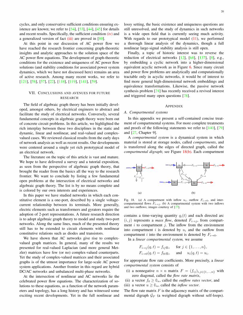
20
cycles, and only conservative sufficient conditions ensuring ex-istence are known; we refer to [54], [53], [44], [45] for detailsand recent results. Specifically, the sufficient condition (iv) anda generalized version of fact (iii) are proved in [80].
At this point in our discussion of AC power flow wehave reached the research frontier concerning graph-theoreticinsights and analytic approaches to the solution space of theAC power flow equations. The development of graph-theoreticconditions for the existence and uniqueness of AC power flowsolutions (and stability conditions for associated power systemdynamics, which we have not discussed here) remains an areaof active research. Among many recent works, we refer to[121], [58], [57], [22], [118], [119], [141], [59].
VII. CONCLUSIONS AND AVENUES FOR FUTURERESEARCH
The field of algebraic graph theory has been initially devel-oped, amongst others, by electrical engineers to abstract andfacilitate the study of electrical networks. Conversely, severalfundamental concepts in algebraic graph theory were born outof concrete circuit problems. In this article, we highlighted therich interplay between these two disciplines in the static anddynamic, linear and nonlinear, and real-valued and complex-valued cases. We reviewed classical results from the early daysof network analysis as well as recent results. Our developmentswere centered around a single yet rich prototypical model ofan electrical network.
The literature on the topic of this article is vast and mature.We hope to have delivered a survey and a tutorial exposition,as seen from the perspective of algebraic graph theory, thatbrought the reader from the basics all the way to the researchfrontier. We want to conclude by listing a few fundamentalopen problems at the intersection of electrical networks andalgebraic graph theory. The list is by no means complete andis colored by our own interests and experiences.
In this paper we have studied networks in which each con-stitutive element is a one-port, described by a single voltage-current relationship between its terminals. More generally,electric elements such as transformers and gyrators require theadoption of 2-port representations. A future research directionis to adopt algebraic graph theory to model and study two-portnetworks. Along the same lines, much of the presented theorystill has to be extended to circuit elements with nonlinearconstitutive relations such as diodes and transistors.
We have shown that AC networks give rise to complex-valued graph matrices. In general, many of the results wepresented for real-valued Laplacian (and more general Met-zler) matrices have few (or no) complex-valued counterparts.Yet the study of complex-valued matrices and their associatedgraphs is of the utmost importance for large-scale AC powersystem applications. Another frontier in this regard are hybridDC/AC networks and unbalanced multi-phase networks.
At the intersection of nonlinear and AC networks lie thecelebrated power flow equations. The characterization of so-lutions to these equations, as a function of the network param-eters and topology, has a long history and has witnessed someexciting recent developments. Yet in the full nonlinear and
lossy setting, the basic existence and uniqueness questions arestill unresolved, and the study of dynamics in such networksis a wide open field that is currently seeing much activity.With regards to our prototypical model (11), we performeda thorough linear analysis of the dynamics, though a fullnonlinear large-signal stability analysis is still open.
Finally, a topic of historic interest was to reverse thereduction of electrical networks [12], [68], [137], [8], e.g.,by embedding a cyclic network into a higher-dimensionalequivalent acyclic network as in Figure 6. Since many circuitand power flow problems are analytically and computationallytractable only in acyclic networks, it would be of interest tofind more general high-dimensional network embeddings andequivalence transformations. Likewise, the passive networksynthesis problem [24] has recently received a revived interestand triggered many open questions [78].
APPENDIX
A. Compartmental systems
In this appendix we present a self-contained concise treat-ment of compartmental systems. For more complete treatmentsand proofs of the following statements we refer to [140], [79]and [27, Chapter 9].
A compartmental system is a dynamical system in whichmaterial is stored at storage nodes, called compartments, andis transferred along the edges of directed graph, called thecompartmental digraph; see Figure 18(b). Each compartment
Fj!iFi!j
ui Fi!0qi
(a)
F1!2
F2!4F3!2
F4!3
F2!3
u1
u3
F2!0
F4!0
q1
q3
q2
q4
(b)
Fig. 18. (a) A compartment with inflow ui, outflow Fi→0, and inter-compartmental flows Fi→j . (b) A compartmental system with two inflowsand two outflows; images courtesy of [27].
contains a time-varying quantity qi(t) and each directed arc(i, j) represents a mass flow, denoted Fi→j , from compart-ment i to compartment j. The inflow from the environmentinto compartment i is denoted by ui and the outflow fromcompartment i into the environment is denoted by Fi→0.
In a linear compartmental system, we assume
Fi→j(q, t) = fijqi, for j ∈ {1, . . . , n},Fi→0(q, t) = f0iqi, and ui(q, t) = ui.
for appropriate flow rate coefficients. More precisely, a linearcompartmental system consists of
(i) a nonnegative n × n matrix F = (fij)i,j∈{1,...,n} withzero diagonal, called the flow rate matrix,
(ii) a vector f0 ≥ 0n, called the outflow rates vector, and(iii) a vector u ≥ 0n, called the inflow vector.The flow rate matrix F is the adjacency matrix of the compart-mental digraph GF (a weighted digraph without self-loops).
21
The instantaneous flow balance provides the affine dynamicsof the system:
qi(t) = −(f0i +
n∑
j=1,j 6=ifij
)qi(t) +
n∑
j=1,j 6=ifjiqj(t) + ui.
The compartmental matrix C = (cij)i,j∈{1,...,n} of a linearcompartmental system is a Metzler matrix defined by
cij =
{fji, if i 6= j,
−f0i −∑nh=1,h6=i fih, if i = j.
Equivalently, C = F>−diag(F1n+f0) and q(t) = Cq(t)+u.In the compartmental digraph, a set of compartments S is
outflow-connected if there exists a directed path from everycompartment in S to the environment, that is, to a compart-ment j with a positive flow rate constant f0j > 0. Moreovera set of compartments S is inflow-connected if there exists adirected path from the environment to every compartment inS, that is, from a compartment i with a positive inflow ui > 0.
Recall that, given a digraph G, its condensation is a digraphwhose nodes are the strongly connected components of G andwhose edges are defined by corresponding edges in G.
With these definitions, the following graph-theoretical andalgebraic statements are known to be equivalent:
(i) the system is outflow-connected,(ii) each sink (node without outgoing edges) of the conden-
sation of GF is outflow-connected, and(iii) the compartmental matrix C is Hurwitz.
Theorem A.1 (Asymptotic behavior of compartmental sys-tems): Consider a linear compartmental system (F, f0, u) withcompartmental matrix C and compartmental digraph GF . If thesystem is outflow-connected, then
(i) the compartmental matrix C is invertible,(ii) every solution tends exponentially to the unique equilib-
rium q∗ = −C−1u ≥ 0n, and(iii) in the ith compartment q∗i > 0 if and only if the ith
compartment is inflow-connected to a positive inflow.
B. Proof of Lemma 5.13: Spectrum of the saddle matrix
The following proof adopts elements from [34], [50], [49].Regarding the first statement 1), we resort to a Lyapunov-
based proof. Consider the auxiliary linear dynamical system[x1
x2
]=
[−G −BB> −R
] [x1
x2
]= A
[x1
x2
], (64)
and the Lyapunov function V(x1, x2) = 12‖x1‖2 + 1
2‖x2‖2.The derivative of V(x, y) is given by
V(x1, x2) = −x>1 Gx1 − x>2 Rx2 ≤ 0 .
It follows that the state (x1, x2) is bounded. Thus, the matrixA admits only eigenvalues with strictly negative real part oreigenvalues on the imaginary axis with equal algebraic andgeometric multiplicity.
Statement 2) is a corollary of Proposition 5.12.If G and R are positive definite, then V(x1, x2) is negative
definite. It follows that the dynamics (64) are asymptoticallystable and A is Hurwitz. This proves the third statement 3).
Regarding the fourth statement 4): To prove the first part,we follow the proof method of [34, Lemma 5.3]. Recallfrom statement 1) that the spectrum of A is restricted to theclosed left half-plane. We aim to prove that, under the statedassumptions, no imaginary eigenvalues other than zero canoccur. We reason by contradiction. Let jσ, with σ 6= 0, be animaginary eigenvalue of A with corresponding non-zero eigen-vector x + jy, where x = [x1 x2]>, y = [y1 y2]> ∈ Rn+m.Then the real and imaginary parts of the eigenvalue equation
jσ(x+ jy) = A(x+ jy) =
[−G −BB> −R
] [x1 + jy1
x2 + jy2
]
yield the set of equations
−Gx1 −Bx2 = −σy1, (65a)−Gy1 −By2 = σx1, (65b)
B>x1 −Rx2 = −σy2, (65c)
B>y1 −Ry2 = σx2. (65d)
We pre-multiply equation (65a), respectively (65c), by x>1 , re-spectively by x>2 , and arrive at−x>1 Gx1−x>1 Bx2 = −σx>1 y1,respectively x>2 B
>x1 − x>2 Rx2 = −σx>2 y2. By adding theseequations we get −x>1 Gx1 − x>2 Rx2 = −σ(x>1 y1 + x>2 y2).Via analogous manipulations of equations (65b) and (65d),we obtain −y>1 Gy1 − y>2 Ry2 = σ(x>1 y1 + x>2 y2). These twoconditions imply that
[x1
x2
]> [G
R
] [x1
x2
]= −
[y1
y2
]> [G
R
] [y1
y2
].
Since G and R are positive semi-definite (possibly zeromatrices) by assumption, we obtain x1 ∈ ker(G), y1 ∈ ker(G)and x2 ∈ ker(R), y2 ∈ ker(R). By further using x1 ∈ker(G), y1 ∈ ker(G) in equations (65a) and (65b) we obtain−Bx2 = −σy1 and −By2 = σx1, that is, x1 ∈ Im(B),y1 ∈ Im(B). We have now established that both x1 and y1
belong to ker(G) ∩ Im(B) and therefore x1 = y1 = 0n byassumption. Similarly, we obtain x2 = y2 = 0m. But it isa contraddiction to have x + jy equal to serve since it is aneigenvector.
Now we prove the second part of statement 4). If G ispositive definite, the Schur determinant formula [160] yields
det
([−G −BB> −R
])= det(G) · det(R+B>G−1B) .
Note that det(G) 6= 0. If B has full rank m, i.e., the graph isacyclic (see statement (S1) in Section III), then B>G−1B hasfull rank, and det(R + B>G−1B) 6= 0. Due to these facts,the matrix A has no eigenvalue at zero and is thus Hurwitz.
The first part of the proof of statement 5) is analogous tothat of statement 4). To prove the second part, we assume thatR is positive definite and apply the Schur determinant formula:
det
([−G −BB> −R
])= det(R) · det(G+BR−1B>) .
Note that det(R) 6= 0 and BR−1B> = LR is a Laplacianmatrix associated to a connected graph. If G has at least onediagonal element, then LR + G is a nonsingular matrix, asdiscussed in Section III-7. Due to these facts, the matrix Ahas no eigenvalue at zero and is thus Hurwitz.
22
C. Proof of Proposition 6.2: Local stability of RLC network
Let (V ∗, f∗) be the unique equilibrium point from Propo-sition 6.1, and consider the linearized dynamic model (50).Applying Proposition 5.13 item 5) to the saddle matrix A(V ∗),we find that A(V ∗) will be Hurwitz if
Gii +P ∗i
(V ∗i )2≥ 0 , i ∈ {1, . . . , n} ,
with strict inequality for at least one value of i ∈ {1, . . . , n}.By changing variables as V ∗i = (VI∗)i(1 + δi), the aboveinequalities are equivalently reformulated as
gi +P ∗i
(VI∗)2i (1 + δi)2
≥ 0 , i ∈ {1, . . . , n} ,
again with strict inequality for at least one value of i. Fromthe proof of Proposition 6.1, each component δi of the shiftedpotential variable δ satisfies −δmax ≤ δi ≤ δmax, where δmax
is given as in Proposition 6.1; the result follows by insertingthe lower bound −δmax into the set of inequalities.
D. Proof of Proposition 6.3: Local stability of RC network
We proceed by linearizing the model (12) around theequilibrium point V ∗. The Jacobian matrix of (12) is
J(V ∗) := C−1(−(LR +G)− diag(P ∗) diag(V ∗)−2
)︸ ︷︷ ︸
:=M1
.
Since C is diagonal and the matrix M1 is a symmet-ric Metzler matrix, it follows that J(V ∗) is Hurwitz ifand only if M1 is negative definite. Substituting V ∗ =diag(VI∗)(1n+δ∗) and defining the congruent matrixM2 :=diag(VI∗)M1 diag(VI∗)/4, it follows that M1 is negativedefinite if and only if
M2 = −Pcrit −1
4diag(1n + δ∗)−2 diag(P ∗)
is negative definite, where we have used the definition of Pcrit.Since Pcrit is symmetric and positive definite, by Sylvester’sInertia Theorem [30] M2 is negative definite if and only if
M3 := P−1critM2 = −In −
1
4P−1
crit diag(P ∗) diag(1n + δ∗)−2
︸ ︷︷ ︸:=∆
is Hurwitz. Stability will now follow if ρ(∆) < 1 . Since italways holds that ρ(∆) ≤ ‖∆‖∞, we compute that
‖∆‖∞ ≤1
4‖P−1
crit diag(P ∗)‖∞‖ diag(1n + δ∗)−2‖∞< ‖P−1
crit diag(P ∗)‖∞ < 1 .
where we have used the fact from Proposition 6.1 that δ∗i ∈(− 1
2 ,12 ) for each component i (in particular, we used the lower
bound) and used (47). It follows that ρ(∆) < 1, and thereforethat J(V ∗) is Hurwitz so V ∗ is locally exponentially stable.
REFERENCES
[1] H. Akagi, E. H. Watanabe, and M. Aredes. Instantaneous Power Theoryand Applications to Power Conditioning. John Wiley & Sons, 2017.
[2] M. Altmann. Reinterpreting network measures for models of diseasetransmission. Social Networks, 15(1):1–17, 1993. doi:10.1016/0378-8733(93)90019-H.
[3] C. S. Amin, M. H. Chowdhury, and Y. I. Ismail. Realizable reduc-tion of interconnect circuits including self and mutual inductances.IEEE Transactions on Computer-Aided Design of Integrated Circuitsand Systems, 24(2):271–277, 2005. doi:10.1109/TCAD.2004.840545.
[4] B. D. O. Anderson and S. Vongpanitlerd. Network Analysis andSynthesis. Dover, 2006.
[5] L. Aolaritei, S. Bolognani, and F. Dorfler. Hierarchical and distributedmonitoring of voltage stability in distribution networks. IEEE Transac-tions on Power Systems, October 2017. Conditionally accepted. URL:https://arxiv.org/abs/1710.10544.
[6] G. I. Atabekov. Linear Network Theory. Pergamon Press, 1965.[7] B. Bamieh, M. R. Jovanovic, P. Mitra, and S. Patterson. Coherence
in large-scale networks: Dimension-dependent limitations of localfeedback. IEEE Transactions on Automatic Control, 57(9):2235–2249,2012. doi:10.1109/TAC.2012.2202052.
[8] V. V. Bapeswara Rao and V. K. Aatre. Mesh-star transformation. Elec-tronics Letters, 10(6):73–74, 1974. doi:10.1049/el:19740056.
[9] N. Barabanov, R. Ortega, R. Grino, and B. Polyak. On existenceand stability of equilibria of linear time-invariant systems with con-stant power loads. IEEE Transactions on Circuits and Systems I:Fundamental Theory and Applications, 63(1):114–121, 2016. doi:10.1109/TCSI.2015.2497559.
[10] P. Barooah and J. P. Hespanha. Estimation on graphs from relativemeasurements. IEEE Control Systems, 27(4):57–74, 2007. doi:10.1109/MCS.2007.384125.
[11] M. Bazrafshan and N. Gatsis. Convergence of the Z-bus method forthree-phase distribution load-flow with ZIP loads. IEEE Transactionson Power Systems, 33(1):153–165, 2018. doi:10.1109/TPWRS.2017.2703835.
[12] S. Bedrosian. Converse of the star-mesh transformation. IRE Transac-tions on Circuit Theory, 8(4):491–493, 1961. doi:10.1109/TCT.1961.1086832.
[13] J. A. Belk, W. Inam, D. J. Perreault, and K. Turitsyn. Stability andcontrol of ad hoc DC microgrids. In IEEE Conf. on Decision andControl, pages 3271–3278, Las Vegas, NV, USA, December 2016.doi:10.1109/CDC.2016.7798761.
[14] M. Benzi, G. H. Golub, and J. Liesen. Numerical solution of saddlepoint problems. Acta Numerica, 14:1–137, 2005. doi:10.1017/S0962492904000212.
[15] M. Benzi and N. Razouk. Decay bounds and o(n) algorithms forapproximating functions of sparse matrices. Electronic Transactionson Numerical Analysis, 28:16–39, 2007. URL: http://etna.mcs.kent.edu/vol.28.2007-2008/pp16-39.dir/pp16-39.pdf.
[16] N. Biggs. Algebraic Graph Theory. Cambridge University Press, 2edition, 1994.
[17] N. Biggs. Algebraic potential theory on graphs. Bulletin of theLondon Mathematical Society, 29(6):641–682, 1997. doi:10.1112/S0024609397003305.
[18] D. A. Bini and B. Meini. The cyclic reduction algorithm: from Poissonequation to stochastic processes and beyond. Numerical Algorithms,51(1):23–60, 2009. doi:10.1007/s11075-008-9253-0.
[19] B. Bollobas. Modern Graph Theory. Springer, 1998.[20] S. Bolognani and F. Dorfler. Fast power system analysis via implicit
linearization of the power flow manifold. In Allerton Conf. on Commu-nications, Control and Computing, pages 402–409, Allerton, IL, USA,September 2015. doi:10.1109/ALLERTON.2015.7447032.
[21] S. Bolognani and S. Zampieri. A distributed control strategy forreactive power compensation in smart microgrids. IEEE Transactionson Automatic Control, 58(11):2818–2833, 2013. doi:10.1109/TAC.2013.2270317.
[22] S. Bolognani and S. Zampieri. On the existence and linear approx-imation of the power flow solution in power distribution networks.IEEE Transactions on Power Systems, 31(1):163–172, 2016. doi:10.1109/TPWRS.2015.2395452.
[23] L. Borcea, V. Druskin, and F. G. Vasquez. Electrical impedancetomography with resistor networks. Inverse Problems, 24(3):035013,2008. doi:10.1088/0266-5611/24/3/035013.
23
[24] R. Bott and R. J. Duffin. Impedance synthesis without use oftransformers. Journal of Applied Physics, 20(8):816–816, 1949. doi:10.1063/1.1698532.
[25] R. K. Brayton and J. K. Moser. A theory of nonlinear networks. I.Quarterly of Applied Mathematics, 22(1):1–33, 1964. doi:10.1090/qam/169746.
[26] R. K. Brayton and J. K. Moser. A theory of nonlinear networks. II.Quarterly of Applied Mathematics, 22(2):81–104, 1964. doi:10.1090/qam/169747.
[27] F. Bullo. Lectures on Network Systems. Version 0.96, January 2018.With contributions by J. Cortes, F. Dorfler, and S. Martınez. URL:http://motion.me.ucsb.edu/book-lns.
[28] S. Y. Caliskan and P. Tabuada. Towards Kron reduction of generalizedelectrical networks. Automatica, 50(10):2586–2590, 2014. doi:10.1016/j.automatica.2014.08.017.
[29] R. Carli, F. Garin, and S. Zampieri. Quadratic indices for the analysisof consensus algorithms. In IEEE Information Theory and ApplicationsWorkshop, pages 96–104, San Diego, CA, USA, February 2009. doi:10.1109/ITA.2009.5044929.
[30] D. Carlson and H. Schneider. Inertia theorems for matrices: Thesemidefinite case. Journal of Mathematical Analysis and Applications,6:430–446, 1963.
[31] A. Carmona, A. M. Encinas, and M. Mitjana. Effective resistancesfor ladder-like chains. International Journal of Quantum Chemistry,114(24):1670–1677, 2014. doi:10.1002/qua.24740.
[32] K. Cavanagh, J. A. Belk, and K. Turitsyn. Transient stability guaranteesfor ad hoc DC microgrids. IEEE Control Systems Letters, 2(1):139–144, 2018. doi:10.1109/LCSYS.2017.2764441.
[33] P. Chebotarev. Comments on ”Consensus and cooperation in networkedmulti-agent systems”. Proceedings of the IEEE, 98(7):1353–1354,2010. doi:10.1109/JPROC.2010.2049911.
[34] A. Cherukuri, B. Gharesifard, and J. Cortes. Saddle-point dynamics:Conditions for asymptotic stability of saddle points. SIAM Journalon Control and Optimization, 55(1):486–511, 2017. doi:10.1137/15M1026924.
[35] H.-D. Chiang. Direct Methods for Stability Analysis of Electric PowerSystems. John Wiley & Sons, 2011.
[36] L. O. Chua. Introduction to Nonlinear Network Theory. McGraw-Hill,1969.
[37] L. O. Chua, C. A. Desoer, and E. S. Kuh. Linear and NonlinearCircuits. McGraw-Hill, 1987.
[38] T. Coletta and P. Jacquod. Performance measures in electric powernetworks under line contingencies, 2017. URL: https://arxiv.org/abs/1711.10348.
[39] M. Colombino, D. Groß, and F. Dorfler. Global phase and voltagesynchronization for power inverters: a decentralized consensus-inspiredapproach. In IEEE Conf. on Decision and Control, pages 5690–5695,Melbourne, Australia, December 2017. doi:10.1109/CDC.2017.8264518.
[40] E. Cotilla-Sanchez, P. D. H. Hines, C. Barrows, and S. Blumsack. Com-paring the topological and electrical structure of the North Americanelectric power infrastructure. IEEE Systems Journal, 6(4):616–626,2012. doi:10.1109/JSYST.2012.2183033.
[41] E. B. Curtis and J. A. Morrow. Inverse Problems for ElectricalNetworks. World Scientific Publishing, 2000.
[42] C. De Persis, E. R. A. Weitenberg, and F. Dorfler. A power consensusalgorithm for DC microgrids. Automatica, February 2017. Submitted.URL: https://arxiv.org/pdf/1611.04192.pdf.
[43] R. C. Degeneff, M. R. Gutierrez, S. J. Salon, D. W. Burow, and R. J.Nevins. Kron’s reduction method applied to the time stepping finiteelement analysis of induction machines. IEEE Transactions on EnergyConversion, 10(4):669–674, 2002. doi:10.1109/60.475837.
[44] R. Delabays, T. Coletta, and P. Jacquod. Multistability of phase-locking and topological winding numbers in locally coupled Kuramotomodels on single-loop networks. Journal of Mathematical Physics,57(3):032701, 2016. doi:10.1063/1.4943296.
[45] R. Delabays, T. Coletta, and P. Jacquod. Multistability of phase-locking in equal-frequency Kuramoto models on planar graphs. Journalof Mathematical Physics, 58(3):032703, 2017. doi:10.1063/1.4978697.
[46] S. Demko, W. F. Moss, and P. W. Smith. Decay rates for inverses ofband matrices. Mathematics of Computation, 43(168):491–499, 1984.URL: http://www.jstor.org/stable/2008290.
[47] S. V. Dhople, B. B. Johnson, F. Dorfler, and A. O. Hamadeh. Syn-chronization of nonlinear circuits in dynamic electrical networks withgeneral topologies. IEEE Transactions on Circuits and Systems I:
Regular Papers, 61(9):2677–2690, 2014. doi:10.1109/TCSI.2014.2332250.
[48] I. Dobson. Voltages across an area of a network. IEEE Transactionson Power Systems, 27(2):993–1002, 2011. doi:10.1109/TPWRS.2011.2168985.
[49] F. Dorfler. Lecture Notes on ”Circuits & Power Grids”, 2017. Part ofthe ”Advanced Topics in Control” Course 2017. URL: http://control.ee.ethz.ch/∼floriand/docs/Teaching/ATIC 2017/Circuits Lecture.pdf.
[50] F. Dorfler. Lecture Notes on ”Distributed Consensus-Based Opti-mization”, 2017. Part of the ”Advanced Topics in Control” Course2017. URL: http://control.ee.ethz.ch/∼floriand/docs/Teaching/ATIC2017/Optimization Lecture.pdf.
[51] F. Dorfler and F. Bullo. Synchronization and transient stability in powernetworks and non-uniform Kuramoto oscillators. SIAM Journal onControl and Optimization, 50(3):1616–1642, 2012. doi:10.1137/110851584.
[52] F. Dorfler and F. Bullo. Kron reduction of graphs with applications toelectrical networks. IEEE Transactions on Circuits and Systems I: Reg-ular Papers, 60(1):150–163, 2013. doi:10.1109/TCSI.2012.2215780.
[53] F. Dorfler and F. Bullo. Synchronization in complex networks of phaseoscillators: A survey. Automatica, 50(6):1539–1564, 2014. doi:10.1016/j.automatica.2014.04.012.
[54] F. Dorfler, M. Chertkov, and F. Bullo. Synchronization in complexoscillator networks and smart grids. Proceedings of the NationalAcademy of Sciences, 110(6):2005–2010, 2013. doi:10.1073/pnas.1212134110.
[55] P. G. Doyle and J. L. Snell. Random Walks and Electric Networks.Mathematical Association of America, 1984.
[56] K. Dvijotham and M. Chertkov. Convexity of structure preservingenergy functions in power transmission: Novel results and applications.In American Control Conference, pages 5035–5042, 2015. doi:10.1109/ACC.2015.7172123.
[57] K. Dvijotham and M. Chertkov. Convexity of structure preservingenergy functions in power transmission: Novel results and applications.In American Control Conference, pages 5035–5042, Chicago, USA,July 2015. doi:10.1109/ACC.2015.7172123.
[58] K. Dvijotham, M. Chertkov, and S. Low. A differential analysis of thepower flow equations. In IEEE Conf. on Decision and Control, pages23–30, Osaka, Japan, December 2015. doi:10.1109/CDC.2015.7402082.
[59] K. Dvijotham, E. Mallada, and J. W. Simpson-Porco. High-voltagesolution in radial power networks: Existence, properties, and equivalentalgorithms. IEEE Control Systems Letters, 1(2):322–327, 2017. doi:10.1109/LCSYS.2017.2717578.
[60] G. Escobar, A. J. van der Schaft, and R. Ortega. A Hamiltonianviewpoint in the modeling of switching power converters. Auto-matica, 35(3):445–452, 1999. doi:10.1016/S0005-1098(98)00196-4.
[61] F. Fagnani and P. Frasca. Introduction to Averaging Dynamics overNetworks. Springer, 2017. doi:10.1007/978-3-319-68022-4.
[62] Y. Fan. Schur complements and its applications to symmetric non-negative and Z-matrices. Linear Algebra and its Applications, 353(1-3):289–307, 2002. doi:10.1016/S0024-3795(02)00327-0.
[63] S. Fiaz, D. Zonetti, R. Ortega, J. M. A. Scherpen, and A. J. van derSchaft. A port-Hamiltonian approach to power network modeling andanalysis. European Journal of Control, 19(6):477–485, 2013. doi:10.1016/j.ejcon.2013.09.002.
[64] M. Fiedler. Algebraic connectivity of graphs. Czechoslovak Mathemat-ical Journal, 23(2):298–305, 1973. URL: http://dml.cz/dmlcz/101168.
[65] M. Fiedler. Inversion of bigraphs and connection with the Gaussianelimination. In Graphs, Hypergraphs and Block Systems, pages 57–68,Zielona Gora, Czechoslovakia, 1976.
[66] M. Fiedler. Special Matrices and their Applications in NumericalMathematics. Martinus Nijhoff Publishers, 1986.
[67] S. Fortunato. Community detection in graphs. Physics Reports, 486(3-5):75–174, 2010. doi:10.1016/j.physrep.2009.11.002.
[68] R. Foster. An open question. IRE Transactions on Circuit Theory,8(2):175–175, 1961. doi:10.1109/TCT.1961.1086780.
[69] F. Fouss, A. Pirotte, J. M. Renders, and M. Saerens. Random-walkcomputation of similarities between nodes of a graph with applicationto collaborative recommendation. IEEE Transactions on Knowledgeand Data Engineering, 19(3):355–369, 2007. doi:10.1109/TKDE.2007.46.
[70] A. Ghosh, S. Boyd, and A. Saberi. Minimizing effective resistanceof a graph. SIAM Review, 50(1):37–66, 2008. doi:10.1137/050645452.
24
[71] J. R. Gilbert. Predicting structure in sparse matrix computations.SIAM Journal on Matrix Analysis and Applications, 15(1):62–79, 1994.doi:10.1137/S0895479887139455.
[72] C. D. Godsil and G. F. Royle. Algebraic Graph Theory. Springer,2001.
[73] A. Gomez-Exposito, A. J. Conejo, and C. Canizares, editors. ElectricEnergy Systems: Analysis and Operation. CRC Press, 2017.
[74] D. Groß, C. Arghir, and F. Dorfler. On the steady-state behavior of anonlinear power system model. Automatica, 90:248–254, 2018. doi:10.1016/j.automatica.2017.12.057.
[75] I. Gutman and W. Xiao. Generalized inverse of the Laplacian matrixand some applications. Bulletin (Acadmie Serbe des Sciences et desArts. Classe des sciences mathmatiques et naturelles. Sciences math-matiques), 129(29):15–23, 2004. URL: http://emis.ams.org/journals/BSANU/29/2.html.
[76] H. Hao and P. Barooah. Asymmetric control achieves size-independentstability margin in 1-D flocks. In IEEE Conf. on Decision and Controland European Control Conference, pages 3458–3463, Orlando, FL,USA, December 2011. doi:10.1109/CDC.2011.6160339.
[77] B. D. Hughes. Random Walks and Random Environments. Volume 1:Random Walks. Clarendon Press, Oxford, 1995.
[78] T. H. Hughes and M. C. Smith. On the minimality and uniquenessof the Bott–Duffin realization procedure. IEEE Transactions onAutomatic Control, 59(7):1858–1873, 2014. doi:10.1109/TAC.2014.2312471.
[79] J. A. Jacquez and C. P. Simon. Qualitative theory of compartmental sys-tems. SIAM Review, 35(1):43–79, 1993. doi:10.1137/1035003.
[80] S. Jafarpour and F. Bullo. Synchronization of Kuramoto oscillators viacutset projections. IEEE Transactions on Automatic Control, November2017. Submitted. URL: https://arxiv.org/abs/1711.03711.
[81] D. Janezic, A. Milicevic, S. Nikolic, and N. Trinajstic. Graph-Theoretical Matrices in Chemistry. CRC Press, 2015.
[82] D. Jeltsema. Budeanu’s concept of reactive and distortion powerrevisited. In International School on Nonsinusoidal Currents andCompensation, pages 1–6, Lagow, Poland, June 2015. doi:10.1109/ISNCC.2015.7174697.
[83] D. Jeltsema, R. Ortega, and J. M. A. Scherpen. On passivity and power-balance inequalities of nonlinear RLC circuits. IEEE Transactionson Circuits and Systems I: Fundamental Theory and Applications,50(9):1174–1179, 2003. doi:10.1109/TCSI.2003.816332.
[84] D. Jeltsema and J. M. A. Scherpen. A dual relation between port-Hamiltonian systems and the Brayton-Moser equations for nonlinearswitched RLC circuits. Automatica, 39(6):969–979, 2003. doi:10.1016/S0005-1098(03)00070-0.
[85] D. Jeltsema and J. M. A. Scherpen. Multidomain modeling of nonlinearnetworks and systems. IEEE Control Systems, 29(4):28–59, 2009.doi:10.1109/MCS.2009.932927.
[86] A. E. Kennelly. The equivalence of triangles and three-pointed stars inconducting networks. Electrical World and Engineer, 34(12):413–414,1899.
[87] Gustav Kirchhoff. Uber die Auflosung der Gleichungen, auf welcheman bei der Untersuchung der linearen Verteilung galvanischer Stromegefuhrt wird. Annalen der Physik und Chemie, 148(12):497–508, 1847.doi:10.1002/andp.18471481202.
[88] D. J. Klein and M. Randic. Resistance distance. Journal of Mathemat-ical Chemistry, 12(1):81–95, 1993. doi:10.1007/BF01164627.
[89] G. Kron. Tensor Analysis of Networks. John Wiley & Sons, 1939.[90] P. Kundur. Power System Stability and Control. McGraw-Hill, 1994.[91] J. Lavei, A. Rantzer, and S. Low. Power flow optimization us-
ing positive quadratic programming. IFAC Proceedings Volumes,44(1):10481–10486, 2011. 18th IFAC World Congress. doi:10.3182/20110828-6-IT-1002.02588.
[92] E. Lovisari, F. Garin, and S. Zampieri. Resistance-based performanceanalysis of the consensus algorithm over geometric graphs. SIAMJournal on Control and Optimization, 51(5):3918–3945, 2013. doi:10.1137/110857428.
[93] J. E. Machado, R. Gri, N. Barabanov, R. Ortega, and B. Polyak. Onexistence of equilibria of multi-port linear AC networks with constant-power loads. IEEE Transactions on Circuits and Systems I: Regular Pa-pers, PP(99):1–11, 2017. doi:10.1109/TCSI.2017.2697906.
[94] J. Machowski, J. W. Bialek, and J. R. Bumby. Power System Dynamics.John Wiley & Sons, 2 edition, 2008.
[95] B. M. Maschke, A. J. van der Schaft, and P. C. Breedveld. Anintrinsic Hamiltonian formulation of the dynamics of LC-circuits. IEEETransactions on Circuits and Systems, 42(2):73–82, 1995. doi:10.1109/81.372847.
[96] B. H. McRae, B. G. Dickson, T. H. Keitt, and V. B. Shah. Using circuittheory to model connectivity in ecology, evolution, and conservation.Ecology, 89(10):2712–2724, 2008. doi:10.1890/07-1861.1.
[97] R. Merris. Laplacian matrices of a graph: A survey. Linear Algebraand its Applications, 197:143–176, 1994. doi:10.1016/j.laa.2011.11.0323374.
[98] C. D. Meyer. Stochastic complementation, uncoupling Markov chains,and the theory of nearly reducible systems. SIAM Review, 31(2):240–272, 1989. doi:10.1137/1031050.
[99] C. D. Meyer. Matrix Analysis and Applied Linear Algebra. SIAM,2001.
[100] U. Miekkala. Graph properties for splitting with grounded Laplacianmatrices. BIT Numerical Mathematics, 33(3):485–495, 1993. doi:10.1007/BF01990530.
[101] G. J. Minty. On the axiomatic foundations of the theories of directedlinear graphs, electrical networks and network-programming. Journalof Mathematics and Mechanics, 15(3):485–520, 1966. URL: http://www.jstor.org/stable/24901346.
[102] B. Mohar. The Laplacian spectrum of graphs. In Y. Alavi, G. Chartrand,O. R. Oellermann, and A. J. Schwenk, editors, Graph Theory, Combi-natorics, and Applications, volume 2, pages 871–898. John Wiley &Sons, 1991. URL: http://citeseerx.ist.psu.edu/viewdoc/summary?doi=10.1.1.96.2577.
[103] R. Olfati-Saber, J. A. Fax, and R. M. Murray. Consensus and coop-eration in networked multi-agent systems. Proceedings of the IEEE,95(1):215–233, 2007. doi:10.1109/JPROC.2006.887293.
[104] R. Ortega, A. J. van der Schaft, I. Mareels, and B. Maschke. Puttingenergy back in control. IEEE Control Systems, 21(2):18–33, 2001.doi:10.1109/37.915398.
[105] M. A. Pai. Energy Function Analysis for Power System Stability.Kluwer Academic Publishers, 1989.
[106] C. R. Paul. Modeling electromagnetic interference properties of printedcircuit boards. IBM Journal of Research and Development, 33(1):33–50, 1989. doi:10.1147/rd.331.0033.
[107] J. H. H. Perk and H. Au-Yang. Yang-Baxter equations. In J.-P. Francoise, G. L. Naber, and S. T. Tsun, editors, Encyclopediaof Mathematical Physics, pages 465–473. Elsevier, 2006. doi:10.1016/B0-12-512666-2/00191-7.
[108] N. Perraudin, J. Paratte, D. Shuman, L. Martin, V. Kalofolias, P. Van-dergheynst, and D. K. Hammond. GSPBOX: A toolbox for signal pro-cessing on graphs, August 2014. URL: https://arxiv.org/abs/1408.5781.
[109] M. Pirani and S. Sundaram. On the smallest eigenvalue of groundedLaplacian matrices. IEEE Transactions on Automatic Control,61(2):509–514, 2016. doi:10.1109/TAC.2015.2444191.
[110] B. K. Poolla, S. Bolognani, and F. Dorfler. Optimal placement ofvirtual inertia in power grids. IEEE Transactions on Automatic Control,62(12):6209–6220, 2017. doi:10.1109/TAC.2017.2703302.
[111] M. A. Porter, J.-P. Onnela, and P. J. Mucha. Communities in networks.Notices of the AMS, 56(9):1082–1097, 2009. URL: http://www.ams.org/notices/200909/rtx090901082p.pdf.
[112] A. Rantzer and B. Bernhardsson. Control of convex-monotone systems.In IEEE Conf. on Decision and Control, pages 2378–2383, Los Ange-les, USA, December 2014. doi:10.1109/CDC.2014.7039751.
[113] J. Rommes and W. H. A. Schilders. Efficient methods for large resistornetworks. IEEE Transactions on Computer-Aided Design of IntegratedCircuits and Systems, 29(1):28–39, 2009. doi:10.1109/TCAD.2009.2034402.
[114] D. J. Rose, R. E. Tarjan, and G. S. Lueker. Algorithmic aspects ofvertex elimination on graphs. SIAM Journal on Computing, 5(2):266–283, 1976. doi:10.1137/0205021.
[115] A. Rosen. A new network theorem. Journal of the Institutionof Electrical Engineers, 62(335):916–918, 1924. doi:10.1049/jiee-1.1924.0120.
[116] W. Rudin. Principles of Mathematical Analysis. International Seriesin Pure and Applied Mathematics. McGraw-Hill, 3 edition, 1976.
[117] D. W. C. Shew. XXVII. generalized star and mesh transforma-tions. The London, Edinburgh, and Dublin Philosophical Magazineand Journal of Science, 38(279):267–275, 1947. doi:10.1080/14786444708521594.
[118] J. W. Simpson-Porco. A theory of solvability for lossless power flowequations – Part I: Fixed-point power flow. IEEE Transactions onControl of Network Systems, 2017. To appear. doi:10.1109/TCNS.2017.2711433.
[119] J. W. Simpson-Porco. A theory of solvability for lossless power flowequations – Part II: Conditions for radial networks. IEEE Transactionson Control of Network Systems, 2017. To appear. doi:10.1109/TCNS.2017.2711859.
25
[120] J. W. Simpson-Porco, F. Dorfler, and F. Bullo. Synchronizationand power sharing for droop-controlled inverters in islanded micro-grids. Automatica, 49(9):2603–2611, 2013. doi:10.1016/j.automatica.2013.05.018.
[121] J. W. Simpson-Porco, F. Dorfler, and F. Bullo. Voltage collapse incomplex power grids. Nature Communications, 7(10790), 2016. doi:10.1038/ncomms10790.
[122] J. W. Simpson-Porco, F. Dorfler, and F. Bullo. Voltage stabilizationin microgrids via quadratic droop control. IEEE Transactions onAutomatic Control, 62(7):1239–253, 2017. doi:10.1109/TAC.2016.2585094.
[123] J. W. Simpson-Porco and N. Monshizadeh. Model-free wide-area mon-itoring of power grids via cutset voltages. In IEEE Conf. on Decisionand Control, pages 7508–7513, Las Vegas, NV, USA, December 2016.doi:10.1109/CDC.2016.7799429.
[124] S. Smale. On the mathematical foundations of electrical circuit theory.Journal of Differential Geometry, 7(1-2):193–210, 1972. doi:10.4310/jdg/1214430827.
[125] E. A. Stone and A. R. Griffing. On the Fiedler vectors of graphs thatarise from trees by Schur complementation of the Laplacian. LinearAlgebra and its Applications, 431(10):1869–1880, 2009. doi:10.1016/j.laa.2009.06.024.
[126] E. Tegling, B. Bamieh, and D. F. Gayme. The price of synchrony:Evaluating the resistive losses in synchronizing power networks. IEEETransactions on Control of Network Systems, 2(3):254–266, 2015.doi:10.1109/TCNS.2015.2399193.
[127] B. D. H. Tellegen. A general network theorem, with applications.Philips Research Reports, 7(4):259–269, 1952.
[128] S. Trip, M. Burger, and C. De Persis. An internal model ap-proach to (optimal) frequency regulation in power grids with time-varying voltages. Automatica, 64:240–253, 2016. doi:10.1016/j.automatica.2015.11.021.
[129] M. Tucci, A. Floriduz, S. Riverso, and G. Ferrari-Trecate. Plug-and-play control of AC islanded microgrids with general topology. InEuropean Control Conference, pages 1493–1500, June 2016. doi:10.1109/ECC.2016.7810501.
[130] M. Tyloo, T. Coletta, and P. Jacquod. Robustness of synchrony incomplex networks and generalized Kirchhoff indices. Physical ReviewLetters, 2018. URL: https://arxiv.org/abs/1710.07536.
[131] A. J. van der Schaft. L2-Gain and Passivity Techniques in NonlinearControl, volume 218 of Lecture Notes in Control and InformationSciences. Springer, 1996.
[132] A. J. van der Schaft. Characterization and partial synthesis of thebehavior of resistive circuits at their terminals. Systems & Control Let-ters, 59(7):423–428, 2010. doi:10.1016/j.sysconle.2010.05.005.
[133] A. J. van der Schaft. Modeling of physical network systems. Systems& Control Letters, 2015. doi:10.1016/j.sysconle.2015.08.013.
[134] A. J. van der Schaft. The flow equations of linear resistive electricalnetworks, December 2017. URL: https://arxiv.org/abs/1712.10263.
[135] A. J. van der Schaft and B. M. Maschke. Port-Hamiltonian systems ongraphs. SIAM Journal on Control and Optimization, 51(2):906–937,2013. doi:10.1137/110840091.
[136] E. I. Verriest and J. C. Willems. The behavior of linear time invariantRLC circuits. In IEEE Conf. on Decision and Control, pages 7754–7758, Atlanta, GA, USA, December 2010. doi:10.1109/CDC.2010.5717364.
[137] L. Versfeld. Remarks on star-mesh transformation of electrical net-works. Electronics Letters, 6(19):597–599, 1970. doi:10.1049/el:19700417.
[138] N. K. Vishnoi. Lx = b, Laplacian solvers and their algorithmicapplications. Theoretical Computer Science, 8(1-2):1–141, 2012.doi:10.1561/0400000054.
[139] C. Wagner, W. Kinzelbach, and G. Wittum. Schur-complementmultigrid. Numerische Mathematik, 75(4):523–545, 1997. doi:10.1007/s00211005.
[140] G. G. Walter and M. Contreras. Compartmental Modeling with Net-works. Birkhauser, 1999. doi:10.1007/978-1-4612-1590-5.
[141] C. Wang, A. Bernstein, J. Y. Le Boudec, and M. Paolone. Explicitconditions on existence and uniqueness of load-flow solutions indistribution networks. IEEE Transactions on Smart Grid, 9(2):953–962, 2018. doi:10.1109/TSG.2016.2572060.
[142] C. Wang and Y. Tokad. Polygon to star transformations. IRETransactions on Circuit Theory, 8(4):489–491, 1961. doi:10.1109/TCT.1961.1086831.
[143] J. B. Ward. Equivalent circuits for power-flow studies. Transactions ofthe American Institute of Electrical Engineers, 68(1):373–382, 2009.doi:10.1109/EE.1949.6444973.
[144] L. Weinberg. Network Analysis and Synthesis. R.E. Krieger Pub. Co.,1975.
[145] J. D. Weston. Unification of linear network theory. Journal of theBritish Institution of Radio Engineers, 6(1):4, 1946. doi:10.1049/jbire.1946.0002.
[146] S. Wiggins. Introduction to Applied Nonlinear Dynamic Systems andChaos. Texts in Applied Mathematics. Springer, 2nd edition, 2003.
[147] J. C. Willems. Dissipative dynamical systems–Part I: General theory.Archive for Rational Mechanics and Analysis, 45(5):321–351, 1972.doi:10.1007/BF0027649.
[148] J. C. Willems. Paradigms and puzzles in the theory of dynamicalsystems. IEEE Transactions on Automatic Control, 36(3):259–294,1991. doi:10.1109/9.73561.
[149] J. C. Willems. Terminals and ports. IEEE Circuits and Systems Mag-azine, 10(4):8–26, 2010. doi:10.1109/MCAS.2010.938635.
[150] J. C. Willems and E. I. Verriest. The behavior of resistive circuits. InIEEE Conf. on Decision and Control and Chinese Control Conference,pages 8124–8129, Shanghai, China, December 2009. doi:10.1109/CDC.2009.5400390.
[151] A. N. Willson. On the solutions of equations for nonlinear resistivenetworks. Bell System Technical Journal, 47(8):1755–1773, 1968.doi:10.1002/j.1538-7305.1968.tb00101.x.
[152] C. W. Wu and L. O. Chua. Application of Kronecker products to theanalysis of systems with uniform linear coupling. IEEE Transactionson Circuits and Systems I: Fundamental Theory and Applications,42(10):775–778, 1995. doi:10.1109/81.473586.
[153] W. Xia and M. Cao. Analysis and applications of spectral propertiesof grounded Laplacian matrices for directed networks. Automatica,80:10–16, 2017. doi:10.1016/j.automatica.2017.01.009.
[154] W. Xiao and I. Gutman. Resistance distance and Laplacian spectrum.Theoretical Chemistry Accounts, 110(4):284–289, 2003. doi:10.1007/s00214-003-0460-4.
[155] L. Yen, M. Saerens, and F. Fouss. A link-analysis extension ofcorrespondence analysis for mining relational databases. IEEE Trans-actions on Knowledge and Data Engineering, 23(4):481–495, 2011.doi:10.1109/TKDE.2010.142.
[156] G. F. Young, L. Scardovi, and N. E. Leonard. Robustness of noisyconsensus dynamics with directed communication. In AmericanControl Conference, pages 6312–6317, Baltimore, MD, USA, 2010.doi:10.1109/ACC.2010.5531506.
[157] G. F. Young, L. Scardovi, and N. E. Leonard. A new notion of effectiveresistance for directed graphs – Part I: Definition and properties. IEEETransactions on Automatic Control, 61(7):1727–1736, 2016. doi:10.1109/TAC.2015.2481978.
[158] S. Yu, H. D. Nguyen, and K. S. Turitsyn. Simple certificate ofsolvability of power flow equations for distribution systems. In IEEEPower & Energy Society General Meeting, pages 1–5, Denver, CO,USA, July 2015. doi:10.1109/PESGM.2015.7286371.
[159] C. Zhang, D. Florencio, and P. A. Chou. Graph signal processing–a probabilistic framework. Microsoft Research, Redmond, WA, USA,Tech. Rep. MSR-TR-2015-31, 2015.
[160] F. Zhang. The Schur Complement and Its Applications. Springer, 2005.[161] K. Zhou, J. C. Doyle, and K. Glover. Robust and Optimal Control.
Prentice Hall, 1996.[162] D. Zonetti, R. Ortega, and A. Benchaib. Modeling and control
of HVDC transmission systems from theory to practice and back.Control Engineering Practice, 45:133–146, 2015. doi:10.1016/j.conengprac.2015.09.012.
26
Florian Dorfler (S’09–M’13) is an Assistant Pro-fessor at the Automatic Control Laboratory at ETHZurich. He received his Ph.D. degree in Mechan-ical Engineering from the University of Californiaat Santa Barbara in 2013, and a Diplom degreein Engineering Cybernetics from the University ofStuttgart in 2008. From 2013 to 2014 he was an As-sistant Professor at the University of California LosAngeles. His primary research interests are centeredaround distributed control, complex networks, andcyber-physical systems currently with applications
in energy systems and smart grids. His students were winners or finalists forBest Student Paper awards at the European Control Conference (2013), andthe American Control Conference (2016), and the PES PowerTech Conference2017. His articles received the 2010 ACC Student Best Paper Award, the 2011O. Hugo Schuck Best Paper Award, and the 2012-2014 Automatica Best PaperAward, and the 2016 IEEE Circuits and Systems Guillemin-Cauer Best PaperAward. He is a recipient of the 2009 Regents Special International Fellowship,the 2011 Peter J. Frenkel Foundation Fellowship, and the 2015 UCSB MEBest PhD award.
John W. Simpson-Porco (S’11–M’16) received theB.Sc. degree in Engineering Physics from Queen’sUniversity, Kingston, ON, Canada in 2010, and thePh.D. degree in Mechanical Engineering from theUniversity of California at Santa Barbara, Santa Bar-bara, CA, USA in 2015. He is currently an AssistantProfessor of Electrical and Computer Engineering atthe University of Waterloo, Waterloo, ON, Canada.He was previously a visiting scientist with the Au-tomatic Control Laboratory at ETH Zurich, Zurich,Switzerland. His research focuses on the control
and optimization of multi-agent systems and networks, with applications inmodernized power grids. Prof. Simpson-Porco is a recipient of the 2012–2014IFAC Automatica Prize and the Center for Control, Dynamical Systems andComputation Best Thesis Award and Outstanding Scholar Fellowship.
Francesco Bullo (S’95-M’99-SM’03-F’10) is a Pro-fessor with the Mechanical Engineering Departmentand the Center for Control, Dynamical Systemsand Computation at the University of California,Santa Barbara. He was previously associated withthe University of Padova, the California Instituteof Technology, and the University of Illinois. Hisresearch interests focus on network systems anddistributed control with application to robotic co-ordination, power grids and social networks. He isthe coauthor of Geometric Control of Mechanical
Systems (Springer, 2004) and Distributed Control of Robotic Networks(Princeton, 2009); his forthcoming ”Lectures on Network Systems” is avail-able on his website. He received best paper awards for his work in IEEEControl Systems, Automatica, SIAM Journal on Control and Optimization,IEEE Transactions on Circuits and Systems, and IEEE Transactions on Controlof Network Systems. He is a Fellow of IEEE and IFAC. He has served onthe editorial boards of IEEE, SIAM, and ESAIM journals, and will serve asIEEE CSS President in 2018.