electrical machines and drives
TRANSCRIPT

5/17/2018 Electrical Machines and Drives - slidepdf.com
http://slidepdf.com/reader/full/electrical-machines-and-drives-55ab59315f602 1/123
Notes for an Introductory Course
On Electrical Machines
and Drives
E.G.Strangas
MSU Electrical Machines and Drives Laboratory

5/17/2018 Electrical Machines and Drives - slidepdf.com
http://slidepdf.com/reader/full/electrical-machines-and-drives-55ab59315f602 2/123
5/17/2018 Electrical Machines and Drives - slidepdf.com
http://slidepdf.com/reader/full/electrical-machines-and-drives-55ab59315f602 3/123
Contents
Preface ix
1 Three Phase Circuits and Power 1
1.1 Electric Power with steady state sinusoidal quantities 11.2 Solving 1-phase problems 5
1.3 Three-phase Balanced Systems 6
1.4 Calculations in three-phase systems 9
2 Magnetics 15
2.1 Introduction 15
2.2 The Governing Equations 15
2.3 Saturation and Hysteresis 19
2.4 Permanent Magnets 21
2.5 Faraday’s Law 222.6 Eddy Currents and Eddy Current Losses 25
2.7 Torque and Force 27
3 Transformers 29
3.1 Description 29
3.2 The Ideal Transformer 30
3.3 Equivalent Circuit 32
3.4 Losses and Ratings 36
3.5 Per-unit System 37
v

5/17/2018 Electrical Machines and Drives - slidepdf.com
http://slidepdf.com/reader/full/electrical-machines-and-drives-55ab59315f602 4/123
vi CONTENTS
3.6 Transformer tests 403.6.1 Open Circuit Test 41
3.6.2 Short Circuit Test 41
3.7 Three-phase Transformers 43
3.8 Autotransformers 44
4 Concepts of Electrical Machines; DC motors 47
4.1 Geometry, Fields, Voltages, and Currents 47
5 Three-phase Windings 53
5.1 Current Space Vectors 53
5.2 Stator Windings and Resulting Flux Density 555.2.1 Balanced, Symmetric Three-phase Currents 58
5.3 Phasors and space vectors 58
5.4 Magnetizing current, Flux and Voltage 60
6 Induction Machines 63
6.1 Description 63
6.2 Concept of Operation 64
6.3 Torque Development 66
6.4 Operation of the Induction Machine near Synchronous Speed 67
6.5 Leakage Inductances and their Effects 71
6.6 Operating characteristics 72
6.7 Starting of Induction Motors 75
6.8 Multiple pole pairs 76
7 Synchronous Machines and Drives 81
7.1 Design and Principle of Operation 81
7.1.1 Wound Rotor Carrying DC 81
7.1.2 Permanent Magnet Rotor 82
7.2 Equivalent Circuit 82
7.3 Operation of the Machine Connected to a Bus of Constant Voltage
and Frequency 847.4 Operation from a Source of Variable Frequency and Voltage 88
7.5 Controllers for PMAC Machines 94
7.6 Brushless DC Machines 94
8 Line Controlled Rectifiers 99
8.1 1- and 3-Phase circuits with diodes 99
8.2 One -Phase Full Wave Rectifier 100
8.3 Three-phase Diode Rectifiers 102
8.4 Controlled rectifiers with Thyristors 103

5/17/2018 Electrical Machines and Drives - slidepdf.com
http://slidepdf.com/reader/full/electrical-machines-and-drives-55ab59315f602 5/123
CONTENTS vii
8.5 One phase Controlled Rectifiers 1048.5.1 Inverter Mode 104
8.6 Three-Phase Controlled Converters 106
8.7 *Notes 107
9 Inverters 109
9.1 1-phase Inverter 109
9.2 Three-phase Inverters 111

5/17/2018 Electrical Machines and Drives - slidepdf.com
http://slidepdf.com/reader/full/electrical-machines-and-drives-55ab59315f602 6/123

5/17/2018 Electrical Machines and Drives - slidepdf.com
http://slidepdf.com/reader/full/electrical-machines-and-drives-55ab59315f602 7/123
Preface
The purpose of these notes is be used to introduce Electrical Engineering students to Electrical
Machines, Power Electronics and Electrical Drives. They are primarily to serve our students at
MSU: they come to the course on Energy Conversion and Power Electronics with a solid background
in Electric Circuits and Electromagnetics, and many want to acquire a basic working knowledge
of the material, but plan a career in a different area (venturing as far as computer or mechanical
engineering). Other students are interested in continuing in the study of electrical machines and
drives, power electronics or power systems, and plan to take further courses in the field.
Starting from basic concepts, the student is led to understand how force, torque, induced voltages
and currents are developed in an electrical machine. Then models of the machines are developed, in
terms of both simplified equations and of equivalent circuits, leading to the basic understanding of
modern machines and drives. Power electronics are introduced, at the device and systems level, and
electrical drives are discussed.
Equations are kept to a minimum, and in the examples only the basic equations are used to solve
simple problems.
These notes do not aim to cover completely the subjects of Energy Conversion and Power
Electronics, nor to be used as a reference, not even to be useful for an advanced course. They are
meant only to be an aid for the instructor who is working with intelligent and interested students,who are taking their first (and perhaps their last) course on the subject. How successful this endeavor
has been will be tested in the class and in practice.
In the present form this text is to be used solely for the purposes of teaching the introductory
course on Energy Conversion and Power Electronics at MSU.
E.G.STRANGAS
E. Lansing, Michigan and Pyrgos, Tinos
ix

5/17/2018 Electrical Machines and Drives - slidepdf.com
http://slidepdf.com/reader/full/electrical-machines-and-drives-55ab59315f602 8/123
A Note on Symbols
Throughout this text an attempt has been made to use symbols in a consistent way. Hence a script
letter, say v denotes a scalar time varying quantity, in this case a voltage. Hence one can see
v = 5 sin ωt or v = v sin ωt
The same letter but capitalized denotes the rms value of the variable, assuming it is periodic.
Hence:
v =√
2V sinωt
The capital letter, but now bold, denotes a phasor:
V = V ejθ
Finally, the script letter, bold, denotes a space vector, i.e. a time dependent vector resulting from
three time dependent scalars:
v = v1 + v2ejγ + v3ej2γ
In addition to voltages, currents, and other obvious symbols we have:
B Magnetic flux Density (T)
H Magnetic filed intensity (A/m)
Φ Flux (Wb) (with the problem that a capital letter is used to show a time
dependent scalar)
λ, Λ, λλλ flux linkages (of a coil, rms, space vector)
ωs synchronous speed (in electrical degrees for machines with more than
two-poles)
ωo rotor speed (in electrical degrees for machines with more than two-poles)
ωm rotor speed (mechanical speed no matter how many poles)
ωr angular frequency of the rotor currents and voltages (in electrical de-
grees)
T Torque (Nm)
(·), (·) Real and Imaginary part of ·x

5/17/2018 Electrical Machines and Drives - slidepdf.com
http://slidepdf.com/reader/full/electrical-machines-and-drives-55ab59315f602 9/123
1Three Phase Circuits and Power
Chapter Objectives
In this chapter you will learn the following:
• The concepts of power, (real reactive and apparent) and power factor
• The operation of three-phase systems and the characteristics of balanced loads in Y and in ∆
• How to solve problems for three-phase systems
1.1 ELECTRIC POWER WITH STEADY STATE SINUSOIDAL QUANTITIES
We start from the basic equation for the instantaneous electric power supplied to a load as shown in
figure 1.1
¡
¢¡ ¢
£¡ £
¤¡ ¤
+v(t)
i(t)
Fig. 1.1 A simple load
p(t) = i(t) · v(t) (1.1)
1

5/17/2018 Electrical Machines and Drives - slidepdf.com
http://slidepdf.com/reader/full/electrical-machines-and-drives-55ab59315f602 10/123
2 THREE PHASE CIRCUITS AND POWER
where i(t) is the instantaneous value of current through the load and v(t) is the instantaneous valueof the voltage across it.
In quasi-steady state conditions, the current and voltage are both sinusoidal, with corresponding
amplitudes i and v, and initial phases, φi and φv , and the same frequency, ω = 2π/T − 2πf :
v(t) = v sin(ωt + φv) (1.2)
i(t) = i sin(ωt + φi) (1.3)
In this case the rms values of the voltage and current are:
V =
1
T T
0
v [sin(ωt + φv)]2 dt =v√
2(1.4)
I =
1
T
T
0
i [sin(ωt + φi)]2 dt =i√2
(1.5)
and these two quantities can be described by phasors, V = V φv and I = I
φi .
Instantaneous power becomes in this case:
p(t) = 2V I [sin(ωt + φv)sin(ωt + φi)]
= 2V I 1
2[cos(φv − φi) + cos(2ωt + φv + φi)] (1.6)
The first part in the right hand side of equation 1.6 is independent of time, while the second part
varies sinusoidally with twice the power frequency. The average power supplied to the load overan integer time of periods is the first part, since the second one averages to zero. We define as real
power the first part:
P = V I cos(φv − φi) (1.7)
If we spend a moment looking at this, we see that this power is not only proportional to the rms
voltage and current, but also to cos(φv − φi). The cosine of this angle we define as displacement
factor, DF. At the same time, and in general terms (i.e. for periodic but not necessarily sinusoidal
currents) we define as power factor the ratio:
pf =P
V I (1.8)
and that becomes in our case (i.e. sinusoidal current and voltage):
pf = cos(φv − φi) (1.9)
Note that this is not generally the case for non-sinusoidal quantities. Figures 1.2 - 1.5 show the cases
of power at different angles between voltage and current.
We call the power factor leading or lagging, depending on whether the current of the load leads
or lags the voltage across it. It is clear then that for an inductive/resistive load the power factor is
lagging, while for a capacitive/resistive load the power factor is leading. Also for a purely inductive
or capacitive load the power factor is 0, while for a resistive load it is 1.
We define the product of the rms values of voltage and current at a load as apparent power, S :
S = V I (1.10)
5/17/2018 Electrical Machines and Drives - slidepdf.com
http://slidepdf.com/reader/full/electrical-machines-and-drives-55ab59315f602 11/123
ELECTRIC POWER WITH STEADY STATE SINUSOIDAL QUANTITIES 3
0 0.1 0.2 0.3 0.4 0.5 0.6 0.7 0.8 0.9 1−1
−0.5
0
0.5
1
i ( t )
0 0.1 0.2 0.3 0.4 0.5 0.6 0.7 0.8 0.9 1−2
−1
0
1
2
u ( t )
0 0.1 0.2 0.3 0.4 0.5 0.6 0.7 0.8 0.9 1−0.5
0
0.5
1
1.5
p ( t )
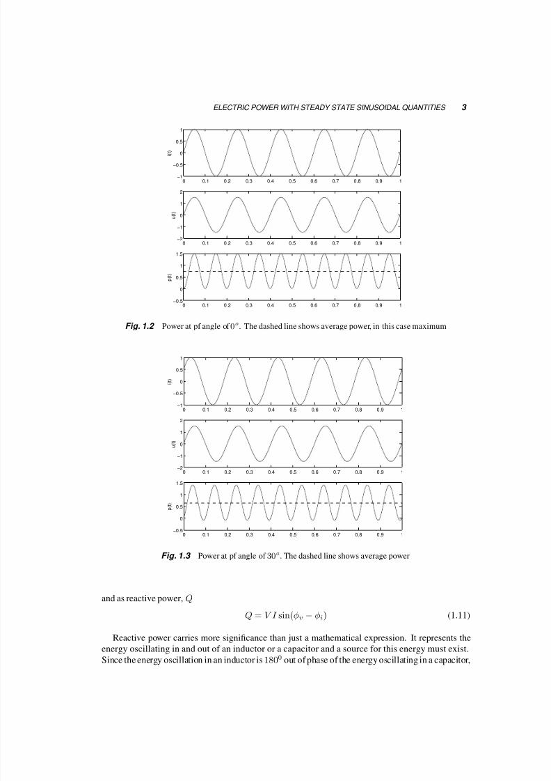
Fig. 1.2 Power at pf angle of 0o. The dashed line shows average power, in this case maximum
0 0.1 0.2 0.3 0.4 0.5 0.6 0.7 0.8 0.9 1−1
−0.5
0
0.5
1
i ( t )
0 0.1 0.2 0.3 0.4 0.5 0.6 0.7 0.8 0.9 1−2
−1
0
1
2
u ( t )
0 0.1 0.2 0.3 0.4 0.5 0.6 0.7 0.8 0.9 1−0.5
0
0.5
1
1.5
p ( t )
Fig. 1.3 Power at pf angle of 30o. The dashed line shows average power
and as reactive power, Q
Q = V I sin(φv − φi) (1.11)
Reactive power carries more significance than just a mathematical expression. It represents the
energy oscillating in and out of an inductor or a capacitor and a source for this energy must exist.
Since the energy oscillation in an inductor is 1800 out of phase of the energy oscillating in a capacitor,

5/17/2018 Electrical Machines and Drives - slidepdf.com
http://slidepdf.com/reader/full/electrical-machines-and-drives-55ab59315f602 12/123
4 THREE PHASE CIRCUITS AND POWER
0 0.1 0.2 0.3 0.4 0.5 0.6 0.7 0.8 0.9 1−1
−0.5
0
0.5
1
i ( t )
0 0.1 0.2 0.3 0.4 0.5 0.6 0.7 0.8 0.9 1−2
−1
0
1
2
u ( t )
0 0.1 0.2 0.3 0.4 0.5 0.6 0.7 0.8 0.9 1−1
−0.5
0
0.5
1
p ( t )
Fig. 1.4 Power at pf angle of 90o. The dashed line shows average power, in this case zero
0 0.1 0.2 0.3 0.4 0.5 0.6 0.7 0.8 0.9 1−1
−0.5
0
0.5
1
i ( t )
0 0.1 0.2 0.3 0.4 0.5 0.6 0.7 0.8 0.9 1−2
−1
0
1
2
u ( t )
0 0.1 0.2 0.3 0.4 0.5 0.6 0.7 0.8 0.9 1
−1.5
−1
−0.5
0
0.5
p ( t )
Fig. 1.5 Power at pf angle of 180o. The dashed line shows average power, in this case negative, the opposite
of that in figure 1.2
the reactive power of the two have opposite signs by convention positive for an inductor, negative for
a capacitor.
The units for real power are, of course, W , for the apparent power V A and for the reactive power
V Ar.

5/17/2018 Electrical Machines and Drives - slidepdf.com
http://slidepdf.com/reader/full/electrical-machines-and-drives-55ab59315f602 13/123
SOLVING 1-PHASE PROBLEMS 5
Using phasors for the current and voltage allows us to define complex power S as:
S = VI∗ (1.12)
= V φvI
−φi (1.13)
and finally
S = P + jQ (1.14)
For example, when
v(t) = (2 · 120 · sin(377t +π
6)V (1.15)
it =
(2 · 5 · sin(377t + π4
)A (1.16)
then S = V I = 120 · 5 = 600W , while pf = cos(π/6 − π/4) = 0.966 leading. Also:
S = VI∗ = 120π/6 5
−π/4 = 579.6W − j155.3V Ar (1.17)
Figure 1.6 shows the phasors for lagging and leading power factors and the corresponding complex
power S.
S
S jQ
jQ
P
P
V
V
I
I
Fig. 1.6 (a) lagging and (b) leading power factor
1.2 SOLVING 1-PHASE PROBLEMS
Based on the discussion earlier we can construct the table below:
Type of load Reactive power Power factor
Reactive Q > 0 lagging
Capacitive Q < 0 leading
Resistive Q = 0 1

5/17/2018 Electrical Machines and Drives - slidepdf.com
http://slidepdf.com/reader/full/electrical-machines-and-drives-55ab59315f602 14/123
6 THREE PHASE CIRCUITS AND POWER
We also notice that if for a load we know any two of the four quantities, S , P , Q, pf , we cancalculate the other two, e.g. if S = 100kV A, pf = 0.8 leading, then:
P = S · pf = 80kW
Q = −S
1 − pf 2 = −60kV Ar , or
sin(φv − φi) = sin [arccos0.8]
Q = S sin(φv − φi)
Notice that here Q < 0, since the pf is leading, i.e. the load is capacitive.
Generally in a system with more than one loads (or sources) real and reactive power balance, but
not apparent power, i.e. P total =
i P i, Qtotal =
i Qi, but S total =
i S i.
In the same case, if the load voltage were V L = 2000V , the load current would be I L = S/V
= 100 · 103/2 · 103 = 50A. If we use this voltage as reference, then:
V = 2000 0V
I = 50φi = 50
36.9oA
S = V I∗ = 2000 0 · 50
−36.9o = P + jQ = 80 · 103W − j60 · 103V Ar
1.3 THREE-PHASE BALANCED SYSTEMS
Compared to single phase systems, three-phase systems offer definite advantages: for the same power
and voltage there is less copper in the windings, and the total power absorbed remains constant rather
than oscillate around its average value.
Let us take now three sinusoidal-current sources that have the same amplitude and frequency, but
their phase angles differ by 1200. They are:
i1(t) =√
2I sin(ωt + φ)
i2(t) =√
2I sin(ωt + φ − 2π
3) (1.18)
i3(t) =√
2I sin(ωt + φ +2π
3)
If these three current sources are connected as shown in figure 1.7, the current returning though node
n is zero, since:
sin(ωt + φ) + sin(ωt − φ +
2π
3 ) + sin(ωt + φ +
2π
3 ) ≡ 0 (1.19)
Let us also take three voltage sources:
va(t) =√
2V sin(ωt + φ)
vb(t) =√
2V sin(ωt + φ − 2π
3) (1.20)
vc(t) =√
2V sin(ωt + φ +2π
3)
connected as shown in figure 1.8. If the three impedances at the load are equal, then it is easy
to prove that the current in the branch n − n is zero as well. Here we have a first reason why

5/17/2018 Electrical Machines and Drives - slidepdf.com
http://slidepdf.com/reader/full/electrical-machines-and-drives-55ab59315f602 15/123
THREE-PHASE BALANCED SYSTEMS 7
n
i1
i2
i3
Fig. 1.7 Zero neutral current in a Y -connected balanced system
n
+ +
+
v
vv
’n’
1
32
Fig. 1.8 Zero neutral current in a voltage-fed, Y -connected, balanced system.
three-phase systems are convenient to use. The three sources together supply three times the power
that one source supplies, but they use three wires, while the one source alone uses two. The wires
of the three-phase system and the one-phase source carry the same current, hence with a three-phase
system the transmitted power can be tripled, while the amount of wires is only increased by 50%.
The loads of the system as shown in figure 1.9 are said to be in Y or star. If the loads are connected
as shown in figure 1.11, then they are said to be connected in Delta, ∆, or triangle. For somebody
who cannot see beyond the terminals of a Y or a ∆ load, but can only measure currents and voltages
there, it is impossible to discern the type of connection of the load. We can therefore consider thetwo systems equivalent, and we can easily transform one to the other without any effect outside the
load. Then the impedances of a Y and its equivalent ∆ symmetric loads are related by:
Z Y =1
3Z ∆ (1.21)
Let us take now a balanced system connected in Y , as shown in figure 1.9. The voltages
between the neutral and each of the three phase terminals are V1n = V φ, V2n = V
φ− 2π3 , and
V3n = V φ+ 2π
3 . Then the voltage between phases 1 and 2 can be shown either through trigonometry
or vector geometry to be:

5/17/2018 Electrical Machines and Drives - slidepdf.com
http://slidepdf.com/reader/full/electrical-machines-and-drives-55ab59315f602 16/123
8 THREE PHASE CIRCUITS AND POWER
V3n
3
2
12
1
V
++
+
-
--
-
+
V1n
2n
V
Fig. 1.9 Y Connected Loads: Voltages and Currents
1n-V
-V3n
V31
V12
V3nV2n
V
-V2n
23 1n
V
Fig. 1.10 Y Connected Loads: Voltage phasors
V12 = V1 − V2 =√
3V φ+π
3 (1.22)
This is shown in the phasor diagrams of figure 1.10, and it says that the rms value of the line-to-line
voltage at a Y load, V ll, is√
3 times that of the line-to-neutral or phase voltage, V ln. It is obvious
that the phase current is equal to the line current in the Y connection. The power supplied to thesystem is three times the power supplied to each phase, since the voltage and current amplitudes and
the phase differences between them are the same in all three phases. If the power factor in one phase
is pf = cos(φv − φi), then the total power to the system is:
S3φ = P 3φ + jQ3φ
= 3V1I∗1
=√
3V llI l cos(φv − φi) + j√
3V llI l sin(φv − φi) (1.23)
Similarly, for a connection in ∆, the phase voltage is equal to the line voltage. On the other hand,
if the phase currents phasors are I12 = I φ, I23 = I
φ− 2π3 and I31 = I
φ+ 2π3 , then the current of

5/17/2018 Electrical Machines and Drives - slidepdf.com
http://slidepdf.com/reader/full/electrical-machines-and-drives-55ab59315f602 17/123
CALCULATIONS IN THREE-PHASE SYSTEMS 9
II
I
1
12
23
31
3I
23
I2
1I
1
I 2
I31-
I-
- I12
23
I
23I
I
I3
12
31I
Fig. 1.11 ∆ Connected Loads: Voltages and Currents
line 1, as shown in figure 1.11 is:
I1 = I12 − I31 =√
3I φ−π
3 (1.24)
To calculate the power in the three-phase, Y connected load,
S3φ = P 3φ + jQ3φ
= 3V1I∗1
=√
3V llI l cos(φv − φi) + j√
3V llI l sin(φv − φi) (1.25)
1.4 CALCULATIONS IN THREE-PHASE SYSTEMS
It is often the case that calculations have to be made of quantities like currents, voltages, and power,
in a three-phase system. We can simplify these calculations if we follow the procedure below:
1. transform the ∆ circuits to Y ,
2. connect a neutral conductor,
3. solve one of the three 1-phase systems,
4. convert the results back to the ∆ systems.
1.4.1 ExampleFor the 3-phase system in figure 1.12 calculate the line-line voltage, real power and power factor at
the load.
First deal with only one phase as in the figure 1.13:
I =120
j1 + 7 + j5= 13.02
−40.6oA
Vln = I Zl = 13.02−40.6o(7 + j5) = 111.97
−5oV
SL,1φ = VL I∗ = 1.186 · 103 + j0.847 · 103
P L1φ = 1.186kW, QL1φ = 0.847kV Ar
pf = cos(−5o − (−40.6o)) = 0.814 lagging

5/17/2018 Electrical Machines and Drives - slidepdf.com
http://slidepdf.com/reader/full/electrical-machines-and-drives-55ab59315f602 18/123
10 THREE PHASE CIRCUITS AND POWER
n
+ +
+
’n’
j 1
7+5jΩ
Ω
120V
Fig. 1.12 A problem with Y connected load.
+
’
Ω
ΩI L
120V
j1
7+j5
Fig. 1.13 One phase of the same load
For the three-phase system the load voltage (line-to-line), and real and reactive power are:
V L,l−l =√
3 · 111.97 = 193.94V
P L,3φ = 3.56kW, QL,3φ = 2.541kVAr
1.4.2 Example
For the system in figure 1.14, calculate the power factor and real power at the load, as well as the
phase voltage and current. The source voltage is 400V line-line.
+ +
+
’n’
j1Ω
18+j6Ω
Fig. 1.14 ∆-connected load

5/17/2018 Electrical Machines and Drives - slidepdf.com
http://slidepdf.com/reader/full/electrical-machines-and-drives-55ab59315f602 19/123
CALCULATIONS IN THREE-PHASE SYSTEMS 11
First we convert the load to Y and work with one phase. The line to neutral voltage of the sourceis V ln = 400/√3 = 231V .
n
+ +
+
’n’
Ω
j1
231V6+j2
Ω
Fig. 1.15 The same load converted to Y
+
’
Ω
j1
231V6+j2
ΩI L
Fig. 1.16 One phase of the Y load
IL =231
j1 + 6 + j2= 34.44
−26.6oA
VL = IL(6 + j2) = 217.8−8.1oV
The power factor at the load is:
pf = cos(φv − φi) = cos(−8.1o + 26.6o) = 0.948lag
Converting back to ∆:
I φ = I L/√
3 = 34.44/√
3 = 19.88A
V ll = 217.8 ·√
3 · 377.22V
At the load
P 3φ =√
3V ll I L pf =√
3 · 377.22 · 34.44 · 0.948 = 21.34kW
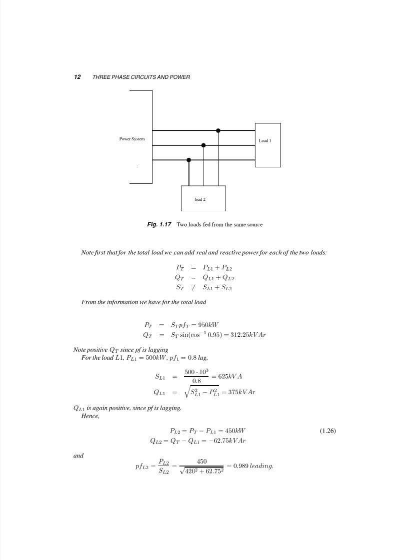
1.4.3 Example
Two loads are connected as shown in figure 1.17. Load 1 draws from the system P L1 = 500kW at
0.8 pf lagging, while the total load is S T = 1000kV A at 0.95 pf lagging. What is the pf of load 2?
5/17/2018 Electrical Machines and Drives - slidepdf.com
http://slidepdf.com/reader/full/electrical-machines-and-drives-55ab59315f602 20/123
12 THREE PHASE CIRCUITS AND POWER
Load 1
load 2
Power System
Fig. 1.17 Two loads fed from the same source
Note first that for the total load we can add real and reactive power for each of the two loads:
P T = P L1 + P L2
QT = QL1 + QL2
S T
= S L1 + S L2
From the information we have for the total load
P T = S T pf T = 950kW
QT = S T sin(cos−1 0.95) = 312.25kV Ar
Note positive QT since pf is lagging
For the load L1 , P L1 = 500kW , pf 1 = 0.8 lag,
S L1 =500 · 103
0.8= 625kV A
QL1 =
S 2L1 − P 2L1 = 375kV Ar
QL1 is again positive, since pf is lagging.
Hence,
P L2 = P T − P L1 = 450kW (1.26)
QL2 = QT − QL1 = −62.75kV Ar
and
pf L2 =P L2S L2
=450√
4202 + 62.752= 0.989 leading.

5/17/2018 Electrical Machines and Drives - slidepdf.com
http://slidepdf.com/reader/full/electrical-machines-and-drives-55ab59315f602 21/123
CALCULATIONS IN THREE-PHASE SYSTEMS 13
Notes
• A sinusoidal signal can be described uniquely by:
1. as e.g. v(t) = 5 sin(2πf t + φv),
2. by its graph,
3. as a phasor and the associated frequency.
one of these descriptions is enough to produce the other two. As an exercise, convert between
phasor, trigonometric expression and time plots of a sinusoid waveform.
• It is the phase difference that is important in power calculations, not phase. The phase alone of
a sinusoidal quantity does not really matter. We need it to solve circuit problems, after we take
one quantity (a voltage or a current) as reference, i.e. we assign to it an arbitrary value, often0. There is no point in giving the phase of currents and voltages as answers, and, especially
for line-line voltages or currents in ∆ circuits, these numbers are often wrong and anyway
meaningless.
• In both 3-phase and 1-phase systems the sum of the real power and the sum of the reactive
power of individual loads are equal respectively to the real and reactive power of the total load.
This is not the case for apparent power and of course not for power factor.
• Of the four quantities, real power, reactive power, apparent power and power factor, any two
describe a load adequately. The other two can be calculated from them.
• To calculate real reactive and apparent Power when using formulae 1.7, 1.10 1.11 we have to
use absolute not complex values of the currents and voltages. To calculate complex powerusing 1.12 we do use complex currents and voltages and find directly both real and reactive
power.
• When solving a circuit to calculate currents and voltages, use complex impedances, currents
and voltages.
• Notice two different and equally correct formulae for 3-phase power.

5/17/2018 Electrical Machines and Drives - slidepdf.com
http://slidepdf.com/reader/full/electrical-machines-and-drives-55ab59315f602 22/123

5/17/2018 Electrical Machines and Drives - slidepdf.com
http://slidepdf.com/reader/full/electrical-machines-and-drives-55ab59315f602 23/123
2 Magnetics
Chapter Objectives
In this chapter you will learn the following:
• How Maxwell’s equations can be simplified to solve simple practical magnetic problems
• The concepts of saturation and hysteresis of magnetic materials
• The characteristics of permanent magnets and how they can be used to solve simple problems
• How Faraday’s law can be used in simple windings and magnetic circuits
• Power loss mechanisms in magnetic materials
• How force and torque is developed in magnetic fields
2.1 INTRODUCTION
Since a good part of electromechanical energy conversion uses magnetic fields it is important early
on to learn (or review) how to solve for the magnetic field quantities in simple geometries and undercertain assumptions. One such assumption is that the frequency of all the variables is low enough
to neglect all displacement currents. Another is that the media (usually air, aluminum, copper, steel
etc.) are homogeneous and isotropic. We’ll list a few more assumptions as we move along.
2.2 THE GOVERNING EQUATIONS
We start with Maxwell’s equations, describing the characteristics of the magnetic field at low fre-
quencies. First we use:
· B = 0 (2.1)
15

5/17/2018 Electrical Machines and Drives - slidepdf.com
http://slidepdf.com/reader/full/electrical-machines-and-drives-55ab59315f602 24/123
16 MAGNETICS
the integral form of which is: B · dA ≡ 0 (2.2)
for any path. This means that there is no source of flux, and that all of its lines are closed.
Secondly we use H · dl =
A
J · dA (2.3)
where the closed loop is defining the boundary of the surface A. Finally, we use the relationship
between H, the strength of the magnetic field, and B, the induction or flux density.
B = µrµ0H (2.4)
where µ0 is the permeability of free space, 4π10−7Tm/A, and µr is the relative permeability of the
material, 1 for air or vacuum, and a few hundred thousand for magnetic steel.
There is a variety of ways to solve a magnetic circuit problem. The equations given above, along
with the conditions on the boundary of our geometry define a boundary value problem. Analytical
methods are available for relatively simple geometries, and numerical methods, like Finite Elements
Analysis, for more complex geometries.
Here we’ll limit ourselves to very simple geometries. We’ll use the equations above, but we’ll add
boundary conditions and some more simplifications. These stem from the assumption of existence
of an average flux path defined within the geometry. Let’s tackle a problem to illustrate it all. In
r
g
i
airgap
Fig. 2.1 A simple magnetic circuit
figure 2.1 we see an iron ring with cross section Ac, average diameter r, that has a gap of length gand a coil around it of N turns, carrying a current i. The additional assumptions we’ll make in order
to calculate the magnetic field density everywhere are:
• The magnetic flux remains within the iron and a tube of air, the airgap, defined by the cross
section of the iron and the length of the gap. This tube is shown in dashed lines in the figure.
• The flux flows parallel to a line, the average flux path, shown in dash-dot.

5/17/2018 Electrical Machines and Drives - slidepdf.com
http://slidepdf.com/reader/full/electrical-machines-and-drives-55ab59315f602 25/123
THE GOVERNING EQUATIONS 17
• Flux density is uniform at any cross-section and perpendicular to it.
Following one flux line, the one coinciding with the average path, we write: H · dl =
J · dA (2.5)
where the second integral extends over any surface (a bubble) terminating on the path of integration.
But equation 2.2, together with the first assumption assures us that for any cross section of the
geometry the flux, Φ =
AcB · dA = Bavg Ac, is constant. Since both the cross section and the flux
are the same in the iron and the air gap, then
Biron = Bair
µironH iron = µairH air
(2.6)
and finally
H iron(2πr − g) + H gap · g = Niµair
µiron(2πr − g) + g
H gap = Ni
l
H r
H y2 y1
H
H l
y y
c
g
Ac
y
Fig. 2.2 A slightly complex magnetic circuit
Let us address one more problem: calculate the magnetic field in the airgap of figure 2.2,
representing an iron core of depth d . Here we have to use two loops like the one above, and we have
5/17/2018 Electrical Machines and Drives - slidepdf.com
http://slidepdf.com/reader/full/electrical-machines-and-drives-55ab59315f602 26/123
18 MAGNETICS
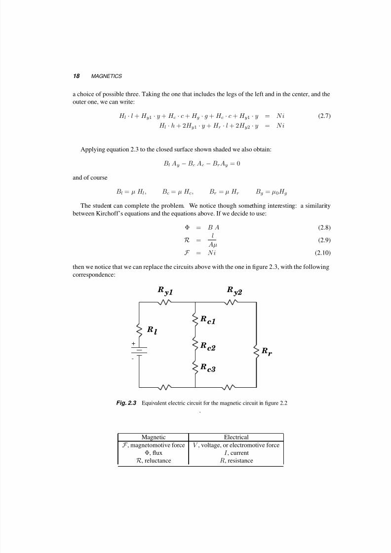
a choice of possible three. Taking the one that includes the legs of the left and in the center, and theouter one, we can write:
H l · l + H y1 · y + H c · c + H g · g + H c · c + H y1 · y = N i (2.7)
H l · h + 2H y1 · y + H r · l + 2H y2 · y = N i
Applying equation 2.3 to the closed surface shown shaded we also obtain:
Bl Ay − Bc Ac − BrAy = 0
and of course
Bl = µ H l, Bc = µ H c, Br = µ H r Bg = µ0H g
The student can complete the problem. We notice though something interesting: a similarity
between Kirchoff’s equations and the equations above. If we decide to use:
Φ = B A (2.8)
R =l
Aµ(2.9)
F = N i (2.10)
then we notice that we can replace the circuits above with the one in figure 2.3, with the following
correspondence:
-
+
R
R
R
R
R
R
y2
rc2
c1
c3
l
y1 R
Fig. 2.3 Equivalent electric circuit for the magnetic circuit in figure 2.2
.
Magnetic Electrical
F , magnetomotive force V , voltage, or electromotive force
Φ, flux I , current
R, reluctance R, resistance

5/17/2018 Electrical Machines and Drives - slidepdf.com
http://slidepdf.com/reader/full/electrical-machines-and-drives-55ab59315f602 27/123
SATURATION AND HYSTERESIS 19
This is of course a great simplification for students who have spent a lot of effort on electricalcircuits, but there are some differences. One is the nonlinearity of the media in which the magnetic
field lives, particularly ferrous materials. This nonlinearity makes the solution of direct problems a
little more complex (problems of the type: for given flux find the necessary current) and the inverse
problems more complex and sometimes impossible to solve without iterations (problems of the type:
for given currents find the flux).
2.3 SATURATION AND HYSTERESIS
Although for free space a equation 2.3 is linear, in most ferrous materials this relationship is nonlinear.
Neglecting for the moment hysteresis, the relationship between H and B can be described by a curve
of the form shown in figure 2.4. From this curve, for a given value of B or H we can find the other
one and calculate the permeability µ = B/H .
Fig. 2.4 Saturation in ferrous materials
In addition to the phenomenon of saturation we have also to study the phenomenon of hysteresis
in ferrous materials. The defining difference is that if saturation existed alone, the flux would be a
unique function of the field intensity. When hysteresis is present, flux density for a give value of
field intensity, H depends also on the history of magnetic flux density, B in it. We can describe the
relationship between field intensity, H and flux density B in homogeneous, isotropic steel with the
curves of 2.5. These curves show that the flux density depends on the history of the magnetization of
the material. This dependence on history is called hysteresis. If we replace the curve with that of the
locus of the extrema, we obtain the saturation curve of the iron, which in itself can be quite useful.
Going back to one of the curves in 2.5, we see that when the current changes sinusoidally between
the two values, i and −i, then the point corresponding to (H, B) travels around the curve. During
this time, power is transferred to the iron, referred to as hysteresis losses, P hyst. The energy of these
losses for one cycle is proportional to the area inside the curve. Hence the power of the losses is
proportional to this surface, the frequency, and the volume of iron; it increases with the maximum
value of B:
P hyst = kf Bx 1 < x < 2 (2.11)
5/17/2018 Electrical Machines and Drives - slidepdf.com
http://slidepdf.com/reader/full/electrical-machines-and-drives-55ab59315f602 28/123
20 MAGNETICS
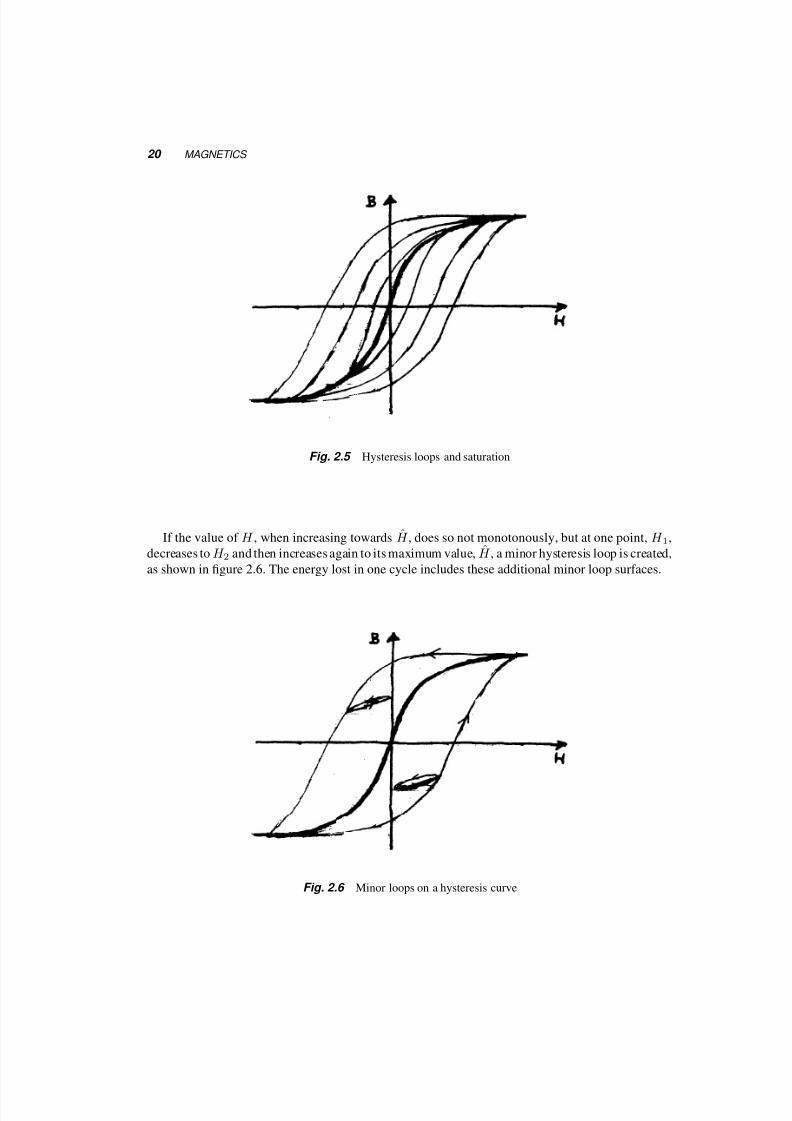
Fig. 2.5 Hysteresis loops and saturation
If the value of H , when increasing towards H , does so not monotonously, but at one point, H 1,
decreases to H 2 and then increases again to its maximum value, H , a minor hysteresis loop is created,
as shown in figure 2.6. The energy lost in one cycle includes these additional minor loop surfaces.
Fig. 2.6 Minor loops on a hysteresis curve

5/17/2018 Electrical Machines and Drives - slidepdf.com
http://slidepdf.com/reader/full/electrical-machines-and-drives-55ab59315f602 29/123
PERMANENT MAGNETS 21
Br
Hc
H
B
Fig. 2.7 Hysteresis curve in magnetic steel
2.4 PERMANENT MAGNETS
If we take a ring of iron with uniform cross section and a magnetic characteristic of the material
that in figure 2.7, and one winding around it, and look only at the second quadrant of the curve, we
notice that for H = 0, i.e. no current in an winding there will be some nonzero flux density, Br. In
addition, it will take current in the winding pushing flux in the opposite direction (negative current)
in order to make the flux zero. The iron in the ring has became a permanent magnet. The value
of the field intensity at this point is −H c. In practice a permanent magnet is operating not at the
second quadrant of the hysteresis loop, but rather on a minor loop, as shown on figure 2.6 that can
be approximated with a straight line. Figure 2.8 shows the characteristics of a variety of permanent
magnets. The curve of a permanent magnet can be described by a straight line in the region of
interest, 2.9, corresponding to the equation:
Bm =H m + H c
H cBr (2.12)
2.4.1 Example
In the magnetic circuit of figure 2.10 the length of the magnet is lm = 1cm , the length of the air gap
is g = 1mm and the length of the iron is li = 20cm. For the magnet Br = 1.1T , H c = 750kA/m.
What is the flux density in the air gap if the iron has infinite permeability and the cross section is
uniform?

5/17/2018 Electrical Machines and Drives - slidepdf.com
http://slidepdf.com/reader/full/electrical-machines-and-drives-55ab59315f602 30/123
22 MAGNETICS
1.4
1.2
1.0
0.8
0.6
(T)
0.4
0.2
-H(kA/m)
Fig. 2.8 Minor loops on a hysteresis curve
Since the cross section is uniform, B is the same everywhere, and there is no current:
H i · 0.2 + H g · g + H m · li = 0
for infinite iron permeability H i = 0 , hence,
Bair1
µog + (Bm − 1.1)
H cBr
li = 0
⇒ B · 795.77 + (B − 1.1) · 6818 = 0B = 0.985T
2.5 FARADAY’S LAW
We’ll see now how voltage is generated in a coil and the effects it may have on a magnetic material.
This theory, along with the previous chapter, is essential in calculating the transfer of energy through
a magnetic field.
First let’s start with the governing equation again. When flux through a coil changes for whatever
reason (e.g. change of the field or relative movement), a voltage is induced in this coil. Figure 2.11

5/17/2018 Electrical Machines and Drives - slidepdf.com
http://slidepdf.com/reader/full/electrical-machines-and-drives-55ab59315f602 31/123
FARADAY’S LAW 23
Br
Hc
H
B
Bm
Hm
Fig. 2.9 Finding the flux density in a permanent magnet
ml
g
Fig. 2.10 Magnetic circuit for Example 2.4.1
shows such a typical case. Faraday’s law relates the electric and magnetic fields. In its integral form:
C
E · dl = − d
dt
A
B · dA (2.13)

5/17/2018 Electrical Machines and Drives - slidepdf.com
http://slidepdf.com/reader/full/electrical-machines-and-drives-55ab59315f602 32/123
24 MAGNETICS
and in the cases we study it becomes:
v(t) =dΦ(t)
dt(2.14)
ΦV
Fig. 2.11 Flux through a coil
If a coil has more than one turns in series, we define as flux linkages of the coil, λ, the sum of the
flux through each turn,λ =
i
Φi (2.15)
and then:
v(t) =dλ(t)
dt(2.16)
2.5.1 Example
For the magnetic circuit shown below µiron = µo ·105 , the air gap is 1mm and the length of the iron
core at the average path is 1m. The cross section of the iron core is 0.04m2. The winding labelled
‘primary’ has 500 turns. A sinusoidal voltage of 60Hz is applied to it. What should be the rms
value of it if the flux density in the iron (rms) is 0.8T ? What is the current in the coil? The voltageinduced in the coil will be
But if B(t) = B sin(2πf t) ⇒ Φ(t) = AB sin(2πf t)
⇒ Φ(t) = 0.04(√
2 · 0.8) sin(377t)W b
e1(t) =dΦ
dt
⇒ e1(t) = 500
0.04√
2 · 0.8 · 377 sin(377t +π
2)
V
⇒ E 1 =e1√
2= 500 · 0.04 · 0.8 · 377 = 6032V
5/17/2018 Electrical Machines and Drives - slidepdf.com
http://slidepdf.com/reader/full/electrical-machines-and-drives-55ab59315f602 33/123
EDDY CURRENTS AND EDDY CURRENT LOSSES 25
g
primary secondary
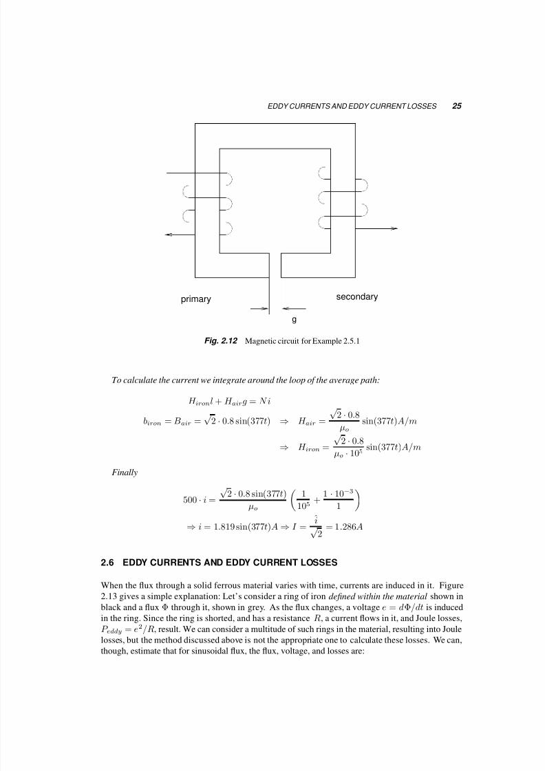
Fig. 2.12 Magnetic circuit for Example 2.5.1
To calculate the current we integrate around the loop of the average path:
H ironl + H airg = N i
biron = Bair =√
2 · 0.8 sin(377t) ⇒ H air =
√2 · 0.8
µosin(377t)A/m
⇒ H iron =
√2 · 0.8
µo · 105sin(377t)A/m
Finally
500 · i =
√2 · 0.8 sin(377t)
µo
1
105+
1 · 10−3
1
⇒i = 1.819sin(377t)A
⇒I =
i
√2
= 1.286A
2.6 EDDY CURRENTS AND EDDY CURRENT LOSSES
When the flux through a solid ferrous material varies with time, currents are induced in it. Figure
2.13 gives a simple explanation: Let’s consider a ring of iron defined within the material shown in
black and a flux Φ through it, shown in grey. As the flux changes, a voltage e = dΦ/dt is induced
in the ring. Since the ring is shorted, and has a resistance R, a current flows in it, and Joule losses,
P eddy = e2/R, result. We can consider a multitude of such rings in the material, resulting into Joule
losses, but the method discussed above is not the appropriate one to calculate these losses. We can,
though, estimate that for sinusoidal flux, the flux, voltage, and losses are:

5/17/2018 Electrical Machines and Drives - slidepdf.com
http://slidepdf.com/reader/full/electrical-machines-and-drives-55ab59315f602 34/123
26 MAGNETICS
¡ ¢
£ ¤
¥§ ¦ ¦ ©
!
Fig. 2.13 Eddy currents in solid iron
Φ = Φsin(ω t) = AB sin(ω t) (2.17)
e = ωΦcos(ω t) = 2πAf B cos(ω t) (2.18)
P eddy = k f 2B2 (2.19)
which tells us that the losses are proportional to the square of both the flux density and frequency.
A typical way to decrease losses is to laminate the material, as shown in figure 2.14, decreasing thepaths of the currents and the total flux through them.
Iron insulation
Fig. 2.14 Laminated steel

5/17/2018 Electrical Machines and Drives - slidepdf.com
http://slidepdf.com/reader/full/electrical-machines-and-drives-55ab59315f602 35/123
TORQUE AND FORCE 27
2.7 TORQUE AND FORCE
Calculating these is quite more complex, since Maxwell’s equations do not refer directly to them.
The most reasonable approach is to start from energy balance. Then the energy in the firles W f is
the sum of the energy that entered through electrical and mechanical sources.
W f =
W e +
W m (2.20)
This in turn can lead to the calculation of the forces since
Kk=1
f kdxk =J
j=1
ej ijdt − dW f (2.21)
Hence for a small movement, dxk, the energies in the equation should be evaluated and from
these, forces (or torques), f k, calculated.
Alternatively, although starting from the same principles, one can use the Maxwell stress tensor
to find forces or torques on enclosed volumes, calculate forces using the Lorenz force equation, here
F = liB, or use directly the balance of energy. Here we’ll use only this last method, e.g. balance
the mechanical and electrical energies.
In a mechanical system with a force F acting on a body and moving it at velocity v in its direction,
the power P mech is
P mech = F · v (2.22)
This eq. 2.22, becomes for a rotating system with torque T , rotating a body with angular velocity
ωmech:
P mech = T · wmech (2.23)On the other hand, an electrical source e, supplying current i to a load provides electrical power
P elec
P elec = e · i (2.24)
Since power has to balance, if there is no change in the field energy,
P elec = P mech ⇒ T · wmech = e · i (2.25)
Notes
•It is more reasonable to solve magnetic circuits starting from the integral form of Maxwell’s
equations than finding equivalent resistance, voltage and current. This also makes it easier touse saturation curves and permanent magnets.
• Permanent magnets do not have flux density equal to BR. Equation 2.12defines the relation
between the variables, flux density Bm and field intensity H m in a permanent magnet.
• There are two types of iron losses: eddy current losses that are proportional to the square of
the frequency and the square of the flux density, and hysteresis losses that are proportional to
the frequency and to some power x of the flux density.

5/17/2018 Electrical Machines and Drives - slidepdf.com
http://slidepdf.com/reader/full/electrical-machines-and-drives-55ab59315f602 36/123

5/17/2018 Electrical Machines and Drives - slidepdf.com
http://slidepdf.com/reader/full/electrical-machines-and-drives-55ab59315f602 37/123
3Transformers
Although transformers have no moving parts, they are essential to electromechanical energy conver-
sion. They make it possible to increase or decrease the voltage so that power can be transmitted at
a voltage level that results in low costs, and can be distributed and used safely. In addition, they can
provide matching of impedances, and regulate the flow of power (real or reactive) in a network.
In this chapter we’ll start from basic concepts and build the equations and circuits corresponding
first to an ideal transformer and then to typical transformers in use. We’ll introduce and work withthe per unit system and will cover three-phase transformers as well.
After working on this chapter, you’ll be able to:
• Choose the correct rating and characteristics of a transformer for a specific application,
• Calculate the losses, efficiency, and voltage regulation of a transformer under specific operating
conditions,
•Experimentally determine the transformer parameters given its ratings.
3.1 DESCRIPTION
When we see a transformer on a utility pole all we see is a cylinder with a few wires sticking out.
These wires enter the transformer through bushings that provide isolation between the wires and
the tank. Inside the tank there is an iron core linking coils, most probably made with copper, and
insulated. The system of insulation is also associated with that of cooling the core/coil assembly.
Often the insulation is paper, and the whole assembly may be immersed in insulating oil, used to
both increase the dielectric strength of the paper and to transfer heat from the core-coil assembly to
the outer walls of the tank to the air. Figure 3.1 shows the cutout of a typical distribution transformer
29
5/17/2018 Electrical Machines and Drives - slidepdf.com
http://slidepdf.com/reader/full/electrical-machines-and-drives-55ab59315f602 38/123
30 TRANSFORMERS
Surge suppressor
CoilCore
LV bushing
HV bushing
oil
Insulating
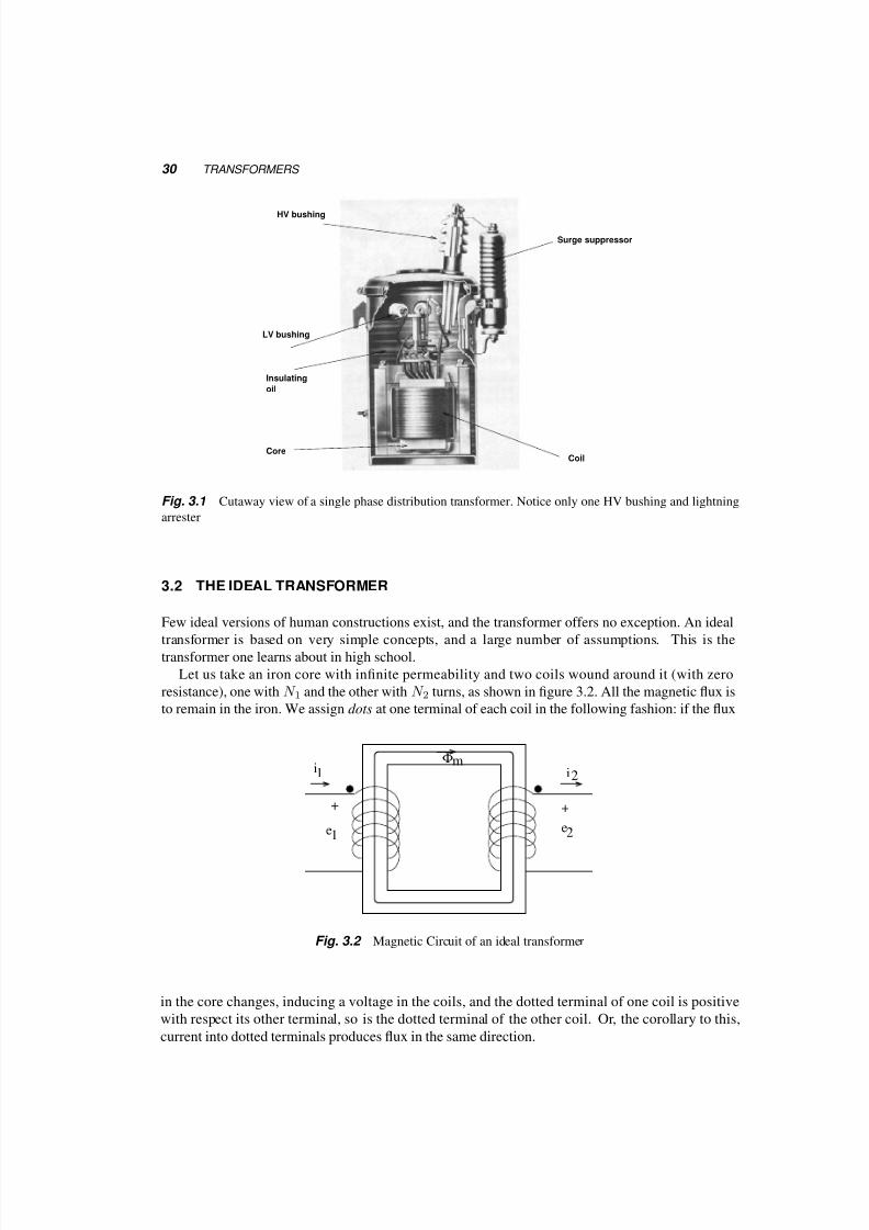
Fig. 3.1 Cutaway view of a single phase distribution transformer. Notice only one HV bushing and lightning
arrester
3.2 THE IDEAL TRANSFORMER
Few ideal versions of human constructions exist, and the transformer offers no exception. An ideal
transformer is based on very simple concepts, and a large number of assumptions. This is thetransformer one learns about in high school.
Let us take an iron core with infinite permeability and two coils wound around it (with zero
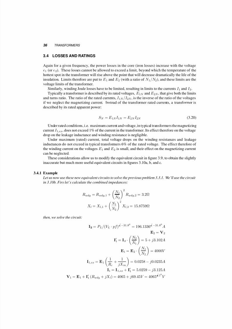
resistance), one with N 1 and the other with N 2 turns, as shown in figure 3.2. All the magnetic flux is
to remain in the iron. We assign dots at one terminal of each coil in the following fashion: if the flux
i2
+
2
m
+
1
1ee
iΦ
Fig. 3.2 Magnetic Circuit of an ideal transformer
in the core changes, inducing a voltage in the coils, and the dotted terminal of one coil is positive
with respect its other terminal, so is the dotted terminal of the other coil. Or, the corollary to this,
current into dotted terminals produces flux in the same direction.

5/17/2018 Electrical Machines and Drives - slidepdf.com
http://slidepdf.com/reader/full/electrical-machines-and-drives-55ab59315f602 39/123
THE IDEAL TRANSFORMER 31
Assume that somehow a time varying flux, Φ(t), is established in the iron. Then the flux linkagesin each coil will be λ1 = N 1Φ(t) and λ2 = N 2Φ(t). Voltages will be induced in these two coils:
e1(t) =dλ1dt
= N 1dΦ
dt(3.1)
e2(t) =dλ2dt
= N 2dΦ
dt(3.2)
and dividing:
e1(t)
e2(t)=
N 1N 2
(3.3)
On the other hand, currents flowing in the coils are related to the field intensity H . If currents
flowing in the direction shown, i1 into the dotted terminal of coil 1, and i2 out of the dotted terminal
of coil 2, then:
N 1 · i1(t) − N 2i2(t) = H · l (3.4)
but B = µironH , and since B is finite and µiron is infinite, then H = 0. We recognize that this is
practically impossible, but so is the existence of an ideal transformer.
Finally:i1i2
=N 2N 1
(3.5)
Equations 3.3 and 3.5 describe this ideal transformer, a two port network. The symbol of a
network that is defined by these two equations is in the figure 3.3. An ideal transformer has an
N N1 2
Fig. 3.3 Symbol for an ideal transformer
interesting characteristic. A two-port network that contains it and impedances can be replaced by an
equivalent other, as discussed below. Consider the circuit in figure 3.4a. Seen as a two port network
E11
2
+
I 1 Z I
+
V2
+
E
1
V
+
N 2N
2
(a)
E1 E2V2
++ +
V1
+
Z’
1 NN 2
(b)
Fig. 3.4 Transferring an impedance from one side to the other of an ideal transformer

5/17/2018 Electrical Machines and Drives - slidepdf.com
http://slidepdf.com/reader/full/electrical-machines-and-drives-55ab59315f602 40/123
32 TRANSFORMERS
with variables v1, i1, v2, i2, we can write:
e1 = u1 − i1Z (3.6)
e2 =N 2N 1
e1 =N 2N 1
u1 − N 2N 1
i1Z (3.7)
v2 = e2 =N 2N 1
e1 =N 2N 1
u1 − i2
N 2N 1
2
Z (3.8)
which could describe the circuit in figure 3.4b. Generally a circuit on a side 1 can be transferred to
side 2 by multiplying its component impedances by (N 2/N 1)2, the voltage sources by (N 2/N 1) and
the current sources by (N 1/N 2), while keeping the topology the same.
3.3 EQUIVALENT CIRCUIT
To develop the equivalent circuit for a transformer we’ll gradually relax the assumptions that we had
first imposed. First we’ll relax the assumption that the permeability of the iron is infinite. In that
case equation 3.4 does not revert to 3.5, but rather it becomes:
N 1i1 − N 2i2 = RΦm (3.9)
where R is the reluctance of the path around the core of the transformer and Φm the flux on this path.
To preserve the ideal transformer equations as part of our new transformer, we can split i1
to two
components: one i1, will satisfy the ideal transformer equation, and the other, i1,ex will just balance
the right hand side. Figure 3.5 shows this.
1
i
+
e ?
i1
1
2
+
--
i1, ex
N
e
N2
21 i
ideal transformer
Fig. 3.5 First step to include magnetizing current
i1 = i1 + i1,ex (3.10)
N 1i1,ex = RΦm (3.11)
N 1i1(t) − N 2i2(t) = H · l (3.12)

5/17/2018 Electrical Machines and Drives - slidepdf.com
http://slidepdf.com/reader/full/electrical-machines-and-drives-55ab59315f602 41/123
EQUIVALENT CIRCUIT 33
We can replace the current source, i1,ex, with something simpler if we remember that the rate of change of flux Φm is related to the induced voltage e1:
e1 = N 1dΦm
dt(3.13)
= N 1d (N 1i1,ex/R)
dt(3.14)
=
N 21R
di1,ex
dt(3.15)
Since the current i1,ex flows through something, where the voltage across it is proportional to its
derivative, we can consider that this something could be an inductance. This idea gives rise to the
equivalent circuit in figure 3.6, where Lm =N 21
R
Let us now relax the assumption that all the flux has
i 1 i 1
e1
+
i 2
+
2
-1 2N N
e
i1, ex
-
ideal transformer
Fig. 3.6 Ideal transformer plus magnetizing branch
to remain in the iron as shown in figure 3.7. Let us call the flux in the iron Φm, magnetizing flux, the
flux that leaks out of the core and links only coil 1, Φl1, leakage flux 1, and for coil 2, Φl2, leakage
flux 2. Since Φl1 links only coil 1, then it should be related only to the current there, and the same
should be true for the second leakage flux.
Fig. 3.7 If the currents in the two windings were to have cancelling values of N · i, then the only flux left
would be the leakage fluxes. This is the case shown here, designed to point out these fluxes.

5/17/2018 Electrical Machines and Drives - slidepdf.com
http://slidepdf.com/reader/full/electrical-machines-and-drives-55ab59315f602 42/123
34 TRANSFORMERS
Φl1 = N 1i1/Rl1 (3.16)Φl2 = N 2i2/Rl2 (3.17)
where Rl1 and Rl2 correspond to paths that are partially in the iron and partially in the air. As these
currents change, so do the leakage fluxes, and a voltage is induced in each coil:
e1 =dλ1dt
= N 1
dΦm
dt
+ N 1
dΦl1
dt= e1 +
N 21Rl1
di1dt
(3.18)
e2 =dλ2dt
= N 2
dΦm
dt
+ N 2
dΦl2
dt= e2 +
N 22Rl2
di2dt
(3.19)
If we define Ll1.
= N 12
Rl1
, Ll2.
=N 21
Rl2
, then we can arrive to the equivalent circuit in figure 3.8. To this
1 e1
i1
+
i1
-
i2
eLl2
-
+
2
+
-1 2
2 v
NN
Ideal transformer
Ll2
i1, ex
v
Fig. 3.8 Equivalent circuit of a transformer plus magnetizing and leakage inductances
circuit we have to add:
1. The winding (ohmic) resistance in each coil, R1,wdg , R2,wdg , with losses P 1,wdg = i21R1,wdg,
P 22,wdg = i22R2,wdg, and
2. some resistance to represent iron losses. These losses (at least the eddy-current ones) are
proportional to the square of the flux. But the flux is proportional to the square of the induced
voltage e1, hence P iron = ke21. Since this resembles the losses of a resistance supplied by
voltage e1, we can develop the equivalent circuit 3.9.
3.3.1 Example
Let us now use this equivalent circuit to solve a problem. Assume that the transformer has a
turns ratio of 4000/120, with R1,wdg = 1.6Ω , R2,wdg = 1.44mΩ , Ll1 = 21mH , Ll2 = 19µH ,Rc = 160kΩ , Lm = 450H . assume that the voltage at the low voltage side is 60Hz , V 2 = 120V ,and the power there is P 2 = 20kW , at pf = 0.85 lagging. Calculate the voltage at the high voltage
side and the efficiency of the transformer.
X m = Lm ∗ 2π60 = 169.7kΩ
X 1 = 7.92Ω
X 2 = 7.16mΩ

5/17/2018 Electrical Machines and Drives - slidepdf.com
http://slidepdf.com/reader/full/electrical-machines-and-drives-55ab59315f602 43/123
EQUIVALENT CIRCUIT 35
2
-
2
-
+
v
+ +
1 Rce
N
el2
L
i
Rwdg,1L
l2
1 1
1 v
-
+Rwdg, 2
2N
1
i1, ex
Ideal transformer
N1 : N2
e2
ii 1
++ R wdg,2
2
+
v1
R
LmR c
L L l2wdg,1 l1
2
ve1
+
(a)
Fig. 3.9 Equivalent circuit for a real transformer
From the power the load:
I2 = P L/(V L pf )−31.80
= 196.1336−31.80
A
E2 = V2 + I2 (Rwdg,2 + jX l2) = 120.98 + j1.045V
E1 =
N 1N 2
E2 = 4032.7 + j34.83V
I1 =
N 2N 1
I2 = 5.001 − j3.1017A
I1,ex = E1
1
Rc+
1
jX m
= 0.0254 − j0.0236A
I1 = I1,ex + I1 = 5.0255 − j3.125A
V1 = E1 + I1 (Rwdg,1 + jX l,1) = 4065.5 + j69.2V = 4066 0.90V
The power losses are concentrated in the windings and core:
P wdg,2 = I 22Rwdg,2 = 196.132 · 1.44 · 10−3 = 55.39W
P wdg,1 = I 21Rwdg,1 = 5.9182 · 1.6 = 65.37W
P core = E 21/Rc = 4032.82/(160 · 103) = 101.64W
P loss = P wdg,1 + P wdg,2 + P core = 213.08W
η =P out
P in=
P out
(P out + P loss)=
20kW
20kW + 213.08W = 0.9895
5/17/2018 Electrical Machines and Drives - slidepdf.com
http://slidepdf.com/reader/full/electrical-machines-and-drives-55ab59315f602 44/123
36 TRANSFORMERS
3.4 LOSSES AND RATINGS
Again for a given frequency, the power losses in the core (iron losses) increase with the voltage
e1 (or e2). These losses cannot be allowed to exceed a limit, beyond which the temperature of the
hottest spot in the transformer will rise above the point that will decrease dramatically the life of the
insulation. Limits therefore are put to E 1 and E 2 (with a ratio of N 1/N 2), and these limits are the
voltage limits of the transformer.
Similarly, winding Joule losses have to be limited, resulting in limits to the currents I 1 and I 2.
Typically a transformer is described by its rated voltages, E 1N and E 2N , that give both the limits
and turns ratio. The ratio of the rated currents, I 1N /I 2N , is the inverse of the ratio of the voltages
if we neglect the magnetizing current. Instead of the transformer rated currents, a transformer is
described by its rated apparent power:
S N = E 1N I 1N = E 2N I 2N (3.20)
Under rated conditions, i.e. maximum current and voltage, in typical transformers the magnetizing
current I 1,ex, does not exceed 1% of the current in the transformer. Its effect therefore on the voltage
drop on the leakage inductance and winding resistance is negligible.
Under maximum (rated) current, total voltage drops on the winding resistances and leakage
inductances do not exceed in typical transformers 6% of the rated voltage. The effect therefore of
the winding current on the voltages E 1 and E 2 is small, and their effect on the magnetizing current
can be neglected.
These considerations allow us to modify the equivalent circuit in figure 3.9, to obtain the slightly
inaccurate but much more useful equivalent circuits in figures 3.10a, b, and c.
3.4.1 Example
Let us now use these new equivalent circuits to solve the previous problem 3.3.1. We’ll use the circuit
in 3.10b. Firs let’s calculate the combined impedances:
Rwdg = Rwdg,1 +
N 1N 2
2
Rwdg,2 = 3.2Ω
X l = X l,1 +
N 1N 2
2
X l,2 = 15.8759Ω
then, we solve the circuit:
I2
= P L
/(V L ·
pf )−31.80 = 196.1336
−31.80A
E2 = V2
I1 = I2 ·
N 2N 1
= 5 + j3.102A
E1 = E2 ·
N 1N 2
= 4000V
I1,ex = E1
1
Rc+
1
jX m
= 0.0258 − j0.0235A
I1 = I1,ex + I1 = 5.0259 − j3.125A
V1 = E1 + I1 (Rwdg + jX l) = 4065 + j69.45V = 4065 10V

5/17/2018 Electrical Machines and Drives - slidepdf.com
http://slidepdf.com/reader/full/electrical-machines-and-drives-55ab59315f602 45/123
PER-UNIT SYSTEM 37
N1 : N2
l1R Lwdg,1
i1
LmR c e2
i
++ R wdg,2
2
L l2
2
v
+
e1
+
1v
i 1
Lm
Rc
N1 : N2
+
2v
i 2
e2e1
++
1v
’ ’’ + +
l1Lwdg,1 R wdg,2 L l2R
i 1
LmR c
i 2
+
2v
N1 : N2
e1 e2
+ +
’ ’l1R Lwdg,1 R wdg,2 L l2
+
1v
’
’ ’
Fig. 3.10 Simplified equivalent circuits of a transformer
The power losses are concentrated in the windings and core:
P wdg = I 1Rwdg = 110.79W
P core = V 21 /Rc = 103.32W
P loss = P wdg + P core = 214.11W
η =P out
P in=
P out
(P out + P loss)=
20kW
20kW + 221.411W = 0.9894
3.5 PER-UNIT SYSTEM
The idea behind the per unit system is quite simple. We define a base system of quantities, express
everything as a percentage (actually per unit) of these quantities, and use all the power and circuit
equations with these per unit quantities. In the process the ideal transformer in 3.10 disappears.
Working in p.u. has a some other advantages, e.g. the range of values of parameters is almost the
same for small and big transformers.
Working in the per unit system adds steps to the solution process, so one hopes that it simplifies
the solution more than it complicates it. At first attempt, the per unit system makes no sense. Let us
look at an example:

5/17/2018 Electrical Machines and Drives - slidepdf.com
http://slidepdf.com/reader/full/electrical-machines-and-drives-55ab59315f602 46/123
38 TRANSFORMERS
3.5.1 Example
A load has impedance 10 + j5Ω and is fed by a voltage of 100V . Calculate the current and power
at the load.
Solution 1 the current will be
IL =VL
ZL
=100
10 + j5= 8.94
−26.570A
and the power will be
P L = V LI L · pf = 100 · 8.94 · cos(26.57) = 800W
Solution 2 Let’s use the per unit system.
1. define a consistent system of values for base. Let us choose V b = 50V , I b = 10A. This means
that Z b = V b/I b = 5Ω
, and P b = V b · I b = 500W
,Qb = 500V Ar
,S b = 500V A
.
2. Convert everything to pu. V L,pu = V L/Bb = 2 pu , ZL,pu = (10 + j5)/5 = 2 + j1 pu.
3. solve in the pu system.
IL,pu =VL,pu
ZL,pu=
2
2 + j1= 0.894
−26.570 pu
P L,pu = V LpuI L,pu · pf = 2 · 0.894 · cos(26.570) = 1.6 pu
4. Convert back to the SI system
I L = I L,pu · I b = 0.894 · 10 = 8.94A
P l = P L,pu
·P b = 1.6
·500 = 800W
The second solution was a bit longer and appears to not be worth the effort. Let us now apply this
method to a transformer, but be shrewder in choosing our bases. Here we’ll need a base system for
each side of the ideal transformer, but in order for them to be consistent, the ratio of the voltage and
current bases should satisfy:
V 1b
V 2b=
N 1N 2
(3.21)
I 1b
I 2b=
N 2N 1
(3.22)
⇒ S 1b = V 1bI 1b = V 2bI 2b = S 2b (3.23)
i.e. the two base apparent powers are the same, as are the two base real and reactive powers.
We often choose as bases the rated quantities of the transformer on each side, This is convenient,since the transformer most of the time operates at rated voltage (making the pu voltage unity), and
the currents and power are seldom above rated, above 1 pu.
Notice that the base impedances on the two sides are related:
Z 1,b =V 1,b
I 1,b(3.24)
Z 2,b =V 2,b
I 2,b=
N 2N 1
2V 1,b
I 1,b(3.25)
Z 2,b =
N 2N 1
2
Z 1,b (3.26)

5/17/2018 Electrical Machines and Drives - slidepdf.com
http://slidepdf.com/reader/full/electrical-machines-and-drives-55ab59315f602 47/123
PER-UNIT SYSTEM 39
We notice that as we move impedances from the one side of the transformer to the other, they getmultiplied or divided by the square of the turns ratio,
N 2N 1
2, but so does the base impedance, hence
the pu value of an impedance stays the same, regardless on which side it is.
Also we notice, that since the ratio of the voltages of the ideal transformer is E1/E2 = N 1/N 2,
is equal to the ratio of the current bases on the two sides on the ideal transformer, then
E1,pu = E2,pu
and similarly,
I1,pu = I2,pu
This observation leads to an ideal transformer where the voltages and currents on one side are
identical to the voltages and currents on the other side, i.e. the elimination of the ideal transformer,
and the equivalent circuits of fig. 3.11 a, b. Let us solve again the same problem as before, with
l1R Lwdg,1 R wdg,2 L l2LmR c
i 2
+
2v
i 1
’
v1
+
(a)
l1R Lwdg,1 R wdg,2 L l2LmR c
i 2
+
2v
i 1
v1
+’
(b)
Fig. 3.11 Equivalent circuits of a transformer in pu
some added information:
3.5.2 Example
A transformer is rated 30kV A , 4000V /120V , with Rwdg,1 = 1.6Ω , Rwdg,2 = 1.44mΩ , Ll1 =21mH , Ll2 = 19µH , Rc = 160kΩ , Lm = 450H . The voltage at the low voltage side is 60Hz ,
V 2 = 120V , and the power there is P 2 = 20kW , at pf = 0.85 lagging. Calculate the voltage at the
high voltage side and the efficiency of the transformer.
1. First calculate the impedances of the equivalent circuit:
V 1b = 4000V
S 1b = 30kV A
I 1b =30 · 103
4 · 103= 7.5A
Z 1b =V 21b
S 1b= 533Ω
V 2b = 120V
S 2b = S 1b = 30kV A
I 2b =S 2b
V 2b= 250A
Z 2b =V 2b
I 2b= 0.48Ω
5/17/2018 Electrical Machines and Drives - slidepdf.com
http://slidepdf.com/reader/full/electrical-machines-and-drives-55ab59315f602 48/123
40 TRANSFORMERS
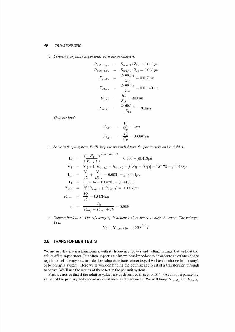
2. Convert everything to per unit: First the parameters:
Rwdg,1,pu = Rwdg,1/Z 1b = 0.003 pu
Rwdg,2,pu = Rwdg,2/Z 2b = 0.003 pu
X l1,pu =2π60Ll1
Z 1b= 0.017 pu
X l2,pu =2π60Ll2
Z 2b= 0.01149 pu
Rc,pu =Rc
Z 1b= 300 pu
X m,pu =2π60Llm
Z 1b= 318 pu
Then the load:
V 2,pu =V 2V 2b
= 1 pu
P 2,pu =P 2S 2b
= 0.6667 pu
3. Solve in the pu system. We’ll drop the pu symbol from the parameters and variables:
I2 =
P 2
V 2 · pf
arccos( pf )
= 0.666 − j0.413 pu
V1 = V2 + I [Rwdg,1 + Rwdg,2 + j(X l1 + X l2)] = 1.0172 + j0.0188 pu
Im = V1Rc
+ V1 jX m
= 0.0034 − j0.0031 pu
I1 = Im + I2 = 0.06701 − j0.416 pu
P wdg = I 22 (Rwdg,1 + Rewg,2) = 0.0037 pu
P core =V 21Rc
= 0.0034 pu
η =P 2
P wdg + P core + P 2= 0.9894
4. Convert back to SI. The efficiency, η , is dimensionless, hence it stays the same. The voltage,
V 1 is
V1 = V1,puV 1b = 4069 10V
3.6 TRANSFORMER TESTS
We are usually given a transformer, with its frequency, power and voltage ratings, but without the
values of its impedances. It is often important to know these impedances, in order to calculate voltage
regulation, efficiency etc., in order to evaluate the transformer (e.g. if we have to choose from many)
or to design a system. Here we’ll work on finding the equivalent circuit of a transformer, through
two tests. We’ll use the results of these test in the per-unit system.
First we notice that if the relative values are as described in section 3.4, we cannot separate the
values of the primary and secondary resistances and reactances. We will lump R1,wdg and R2,wdg

5/17/2018 Electrical Machines and Drives - slidepdf.com
http://slidepdf.com/reader/full/electrical-machines-and-drives-55ab59315f602 49/123
TRANSFORMER TESTS 41
together, as well as X l1 and X l2. This will leave four quantities to be determined, Rwdg , X l, Rc andX m.
3.6.1 Open Circuit Test
We leave one side of the transformer open circuited, while to the other we apply rated voltage (i.e.
V oc = 1 pu) and measure current and power. On the open circuited side of the transformer rated
voltage appears, but we just have to be careful not to close the circuit ourselves. The current that
flows is primarily determined by the impedances X m and Rc, and it is much lower than rated. It is
reasonable to apply this voltage to the low voltage side, since (with the ratings of the transformer in
our example) is it easier to apply 120V , rather than 4000V . We will use these two measurements to
calculate the values of Rc and X m.
Dropping the subscript pu, using the equivalent circuit of figure 3.11b and neglecting the voltage
drop on the horizontal part of the circuit, we calculate:
P oc =V oc
2
Rc=
1
Rc(3.27)
Ioc =V oc
Rc+
V oc
jX m
I oc = 1
1
Rc2 +
1
X m2
(3.28)
Equations 3.27 and 3.28, allow us to use the results of the short circuit test to calculate the vertical
(core) branch of the transformer equivalent circuit.
3.6.2 Short Circuit Test
To calculate the remaining part of the equivalent circuit, i.e the values of Rwdg and X l, we short
circuit one side of the transformer and apply rated current to the other. We measure the voltage of
that side and the power drawn. On the other side, (the short-circuited one) the voltage is of course
zero, but the current is rated. We often apply voltage to the high voltage side, since a) the applied
voltage need not be high and b) the rated current on this side is low.
Using the equivalent circuit of figure 3.11a, we notice that:
P sc = I 2scRwdg = 1 · Rwdg (3.29)
Vsc = Isc (Rwdg + jX l)
V sc = 1 ·
R2wdg + X 2l (3.30)
Equations 3.29 and 3.30 can give us the values of the parameters in the horizontal part of the
equivalent circuit of a transformer.
3.6.1 Example
A 60Hz transformer is rated 30kV A , 4000V /120V . The open circuit test, performed with the high
voltage side open, gives P oc = 100W , I oc = 1.1455A. The short circuit test, performed with the
low voltage side shorted, gives P sc = 180W , V sc = 129.79V . Calculate the equivalent circuit of
the transformer in per unit.

5/17/2018 Electrical Machines and Drives - slidepdf.com
http://slidepdf.com/reader/full/electrical-machines-and-drives-55ab59315f602 50/123
42 TRANSFORMERS
First define bases:
V 1b = 4000V
S 1b = 30kV A
I 1b =30 · 103
4 · 103= 7.5A
Z 1b =V 21b
S 1b= 533Ω
V 2b = 120V
S 2b = S 1b = 30kV A
I 2b =S 1b
V 2b
= 250A
Z 2b =V 1b
I 1b= 0.48Ω
Convert now everything to per unit:
P sc,pu =180
30 · 103= 0.006 ppu
V sc,pu =129.79
4000= 0.0324 pu
P oc,pu =100
30
·103
= 0.003333 pu
I oc,pu = 1.1455250
= 0.0046 pu
Let’s calculate now, dropping the pu subscript:
P sc = I 2scRwdg ⇒ Rwdg = P sc/I 2sc = 1 · P sc = 0.006 pu
|Vsc| = |Isc| · |Rwdg + jX l| = 1 ·
R2wdg + X 2l ⇒ X l =
V 2sc − R2
wdg = 0.0318 pu
P oc =V 2oc
Rc⇒ Rc =
12
P oc= 300 pu
|Ioc| =
Voc
Rc +
Voc
jX m
= 1
R2c +
1
X 2m ⇒ X m =
1 I 2oc − 1
R2c
= 318 pu
A more typical problem is of the type:
3.6.2 Example
A 60Hz transformer is rated 30kV A , 4000V /120V . Its short circuit impedance is 0.0324 pu and the
open circuit current is 0.0046 pu. The rated iron losses are 100W and the rated winding losses are
180W . Calculate the efficiency and the necessary primary voltage when the load at the secondary
is at rated voltage, 20kW at 0.8 pf lagging.

5/17/2018 Electrical Machines and Drives - slidepdf.com
http://slidepdf.com/reader/full/electrical-machines-and-drives-55ab59315f602 51/123
THREE-PHASE TRANSFORMERS 43
Working in pu:Z sc = 0.0324 pu
P sc = Rwdg =180
30 · 103= 6 · 10−3 pu
⇒ X l =
Z 2sc − R2wdg = 0.017 pu
P oc =1
Rc⇒ Rc =
1
P oc=
1
100/30 · 103= 300 pu
I oc =
1
R2c
+1
X 2m⇒ X m = 1
I 2oc − 1
R2c
= 318 pu
Having finished with the transformer data, let us work with the load and circuit. The load power
is 20kW , hence:
P 2 =20 · 103
30 · 103= 0.6667 pu
but the power at the load is:
P 2 = V 2I 2 pf ⇒ 0.6667 = 1 · I 2 · 0.8 ⇒ I 2 = 0.8333 pu
Then to solve the circuit, we work with phasors. We use the voltage V 2 as reference:
V2 = V 2 = 1 pu
I2 = 0.8333 cos−10.8 = 0.6667 − j0.5 pu
V1 = V2 + I2 (Rwdg + jX l) = 1.0199 + j0.00183 pu ⇒ V 1 = 1.02 pu
P wdg = I 22
·Rwdg = 0.0062 pu
P c = V 21 /Rc = 0.034 pu
η =P 2
P 2 + P wdg + P c= 0.986
Finally, we convert the voltage to SI
V 1 = V 1,pu · V b1 = 1.021 · 4000 = 4080V
3.7 THREE-PHASE TRANSFORMERS
We’ll study now three-phase transformers, considering as consisting of three identical one-phase
transformers. This method is accurate as far as equivalent circuits and two-port models are our
interest, but it does not give us insight into the magnetic circuit of the three-phase transformer. Theprimaries and the secondaries of the one-phase transformers can be connected either in ∆ or in Y .In either case, the rated power of the three-phase transformer is three times that of the one-phase
transformers. For ∆ connection,
V ll = V 1φ (3.31)
I l =√
3I 1φ (3.32)
For Y connection
V ll =√
3V 1φ (3.33)
I l = I 1φ (3.34)

5/17/2018 Electrical Machines and Drives - slidepdf.com
http://slidepdf.com/reader/full/electrical-machines-and-drives-55ab59315f602 52/123
44 TRANSFORMERS
2
21
1
1V2
2
2
21
1
1
i
V
i
V
V
ii
V V
i i
(a)
2
1
1 2
2
2
2
21
V1
1
1
i i
V
VV
i
i
V V
i
i
(b)
Fig. 3.12 Y − Y and Y −∆ Connections of three-phase Transformers
2
21
1
1
i i
2
ii
1
V
ii
V
V2V
21
V V
21
(a)
1 2
2i1
1 2
21
1 2
21
i
VV
V
i i
V
VV
ii
(b)
Fig. 3.13 ∆− Y and ∆−∆ Connections of three-phase Transformers
3.8 AUTOTRANSFORMERS
An autotransformer is a transformer where the two windings (of turns N 1 and N 2) are not isolated
from each other, but rather connected as shown in figure 3.14. It is clear form this figure that the

5/17/2018 Electrical Machines and Drives - slidepdf.com
http://slidepdf.com/reader/full/electrical-machines-and-drives-55ab59315f602 53/123
AUTOTRANSFORMERS 45
voltage ratio in an autotransformer is
V 1V 2
=N 1 + N 2
N 2(3.35)
while the current ratio isI 2I 1
=N 1 + N 2
N 2(3.36)
The interesting part is that the coil of turns of N 1 carries current I 1, while the coil of turns N 2 carries
the (vectorial) sum of the two currents, I1−I2. So if the voltage ratio where 1, no current would flow
through that coil. This characteristic leads to a significant reduction in size of an autotransformer
compared to a similarly rated transformer, especially if the primary and secondary voltages are of
the same order of magnitude. These savings come at a serious disadvantage, the loss of isolation
between the two sides.
N
N ¡
V
V ¡
I
I¡
I¡
-I
+
+
Fig. 3.14 An Autotransformer
Notes
•To understand the operation of transformers we have to use both the Biot-Savart Law and
Faraday’s law.
• Most transformers operate under or near rated voltage. As the voltage drop in the leakage
inductance and winding resistances are small, the iron losses under such operation transformer
are close to rated.
• The open- and short-circuit test are just that, tests. They provide the parameters that define the
operation of the transformer.
• Three-phase transformers can be considered to be made of three single-phase transformers for
the purposes of these notes. The main issue then is to calculate the ratings and the voltages
and currents of each.

5/17/2018 Electrical Machines and Drives - slidepdf.com
http://slidepdf.com/reader/full/electrical-machines-and-drives-55ab59315f602 54/123
46 TRANSFORMERS
• Autotransformers are used mostly to vary the voltage a little. It is seldom that an autotrans-former will have a voltage ratio greater than two.

5/17/2018 Electrical Machines and Drives - slidepdf.com
http://slidepdf.com/reader/full/electrical-machines-and-drives-55ab59315f602 55/123
4Concepts of Electrical Machines; DC motors
DC machines have faded from use due to their relatively high cost and increased maintenance
requirements. Nevertheless, they remain good examples for electromechanical systems used for
control. We’ll study DC machines here, at a conceptual level, for two reasons:
1. DC machines although complex in construction, can be useful in establishing the concepts of
emf and torque development, and are described by simple equations.
2. The magnetic fields in them, along with the voltage and torque equations can be used easily to
develop the ideas of field orientation.
In doing so we will develop basic steady-state equations, again starting from fundamentals of the
electromagnetic field. We are going to see the same equations in ‘Brushless DC’ motors, when we
discuss synchronous AC machines.
4.1 GEOMETRY, FIELDS, VOLTAGES, AND CURRENTS
Let us start with the geometry shown in figure 4.1
This geometry describes an outer iron window (stator), through which (i.e. its center part) a
uniform magnetic flux is established, say Φ. How this is done (a current in a coil, or a permanent
magnet) is not important here.
In the center part of the window there is an iron cylinder (called rotor), free to rotate around its
axis. A coil of one turn is wound diametrically around the cylinder, parallel to its axis. As the
cylinder and its coil rotate, the flux through the coil changes. Figure 4.2 shows consecutive locations
of the rotor and we can see that the flux through the coil changes both in value and direction. The
top graph of figure 4.3 shows how the flux linkages of the coil through the coil would change, if the
rotor were to rotate at a constant angular velocity, ω.
λ = Φcos[ωt] (4.1)
47
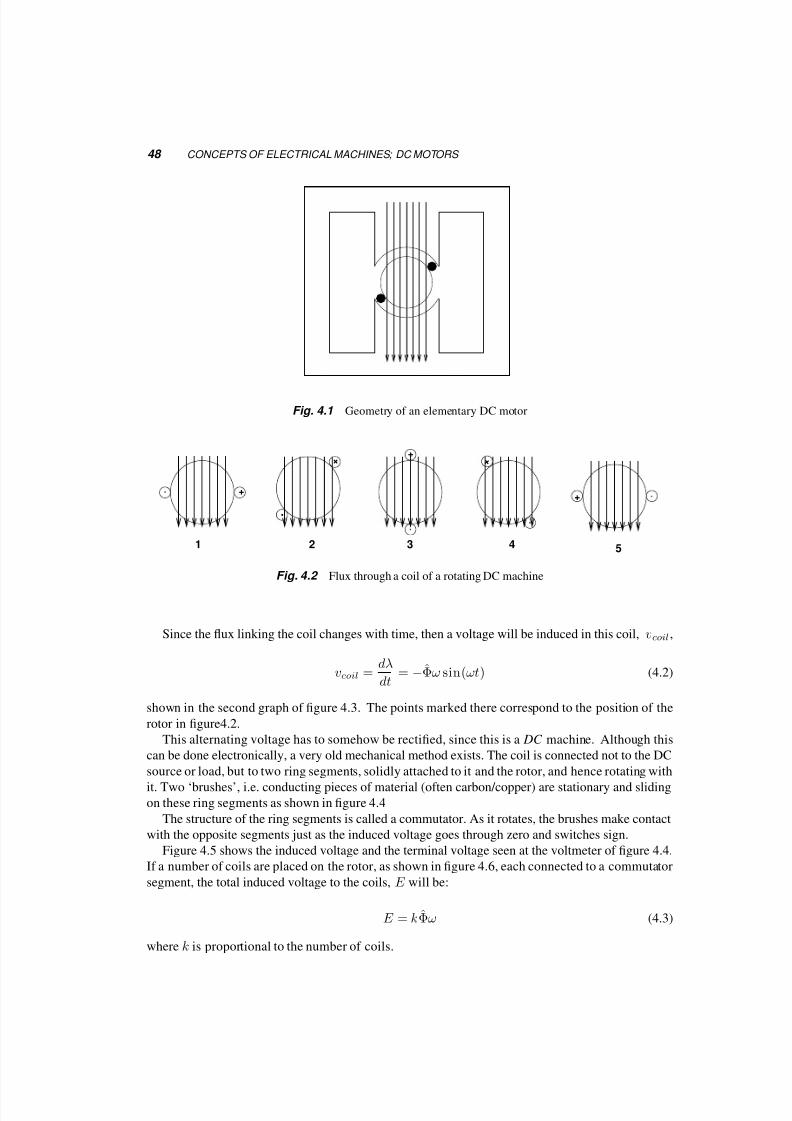
5/17/2018 Electrical Machines and Drives - slidepdf.com
http://slidepdf.com/reader/full/electrical-machines-and-drives-55ab59315f602 56/123
48 CONCEPTS OF ELECTRICAL MACHINES; DC MOTORS
Fig. 4.1 Geometry of an elementary DC motor
+
+
+ +
+
1 2 3 4 5
Fig. 4.2 Flux through a coil of a rotating DC machine
Since the flux linking the coil changes with time, then a voltage will be induced in this coil, vcoil,
vcoil =dλ
dt= −Φω sin(ωt) (4.2)
shown in the second graph of figure 4.3. The points marked there correspond to the position of the
rotor in figure4.2.
This alternating voltage has to somehow be rectified, since this is a DC machine. Although this
can be done electronically, a very old mechanical method exists. The coil is connected not to the DC
source or load, but to two ring segments, solidly attached to it and the rotor, and hence rotating with
it. Two ‘brushes’, i.e. conducting pieces of material (often carbon/copper) are stationary and sliding
on these ring segments as shown in figure 4.4
The structure of the ring segments is called a commutator. As it rotates, the brushes make contact
with the opposite segments just as the induced voltage goes through zero and switches sign.
Figure 4.5 shows the induced voltage and the terminal voltage seen at the voltmeter of figure 4.4.
If a number of coils are placed on the rotor, as shown in figure 4.6, each connected to a commutator
segment, the total induced voltage to the coils, E will be:
E = kΦω (4.3)
where k is proportional to the number of coils.

5/17/2018 Electrical Machines and Drives - slidepdf.com
http://slidepdf.com/reader/full/electrical-machines-and-drives-55ab59315f602 57/123
GEOMETRY, FIELDS, VOLTAGES, AND CURRENTS 49
0 100 200 300 400 500 600 700
−1.5
−1
−0.5
0
0.5
1
1.5
λ c o i l
1
2
3
4
5
0 100 200 300 400 500 600 700
−1.5
−1
−0.5
0
0.5
1
1.5
v c o i l
1
2
3
4
5
Fig. 4.3 Flux and voltage in a coil of the DC machine in 4.2. Points 1 – 5 represent the coil positions.
Going back to equation 2.25,
E · i = T ω (4.4)
kΦωi = T ω (4.5)
T = kΦi (4.6)
If the electrical machine is connected to a load or a source as in figure4.7, the induced voltage and
terminal voltage will be related by:
V term = E − igRwdg for a generator (4.7)
V term = E + imRwdg for a motor (4.8)
4.1.1 Example
A DC motor, when connected to a 100V source and to no load runs at 1200rpm. Its stator resistance
is 2Ω. What should be the torque and current if it is fed from a 220V supply and its speed is
1500rpm? Assume that the field is constant.
The first piece of information gives us the constant k. Since at no load the torque is zero and
T = kΦi = Ki , then the current is zero as well. This means that for this operation:
V = E = kΦω = Kω

5/17/2018 Electrical Machines and Drives - slidepdf.com
http://slidepdf.com/reader/full/electrical-machines-and-drives-55ab59315f602 58/123
50 CONCEPTS OF ELECTRICAL MACHINES; DC MOTORS
Copper Half Ring
Brush
rotating with the
coil
V
Stationary
Coil
B
Fig. 4.4 A coil of a DC motor and a commutator with brushes
0 100 200 300 400 500 600 700
−1.5
−1
−0.5
0
0.5
1
1.5
v c o i l
0 100 200 300 400 500 600 700
−1.5
−1
−0.5
0
0.5
1
1.5
v t e r m
Fig. 4.5 Induced voltage in a coil and terminal voltage in an elementary DC machine
but ω is 1200 rpm, or in SI units:
ω = 12002π
60= 125.66rad/s

5/17/2018 Electrical Machines and Drives - slidepdf.com
http://slidepdf.com/reader/full/electrical-machines-and-drives-55ab59315f602 59/123
GEOMETRY, FIELDS, VOLTAGES, AND CURRENTS 51
+ +
+
+
+
+ +
+
+
--
-
-
-
-
-
-
-
Fig. 4.6 Coils on the rotor of DC machine
wdgR
Source
or
Load
im
gi
E
Fig. 4.7 Circuit with a DC machine
And
100V = K · 125.66 ⇒ K = 0.796V s
At the operating point of interest:
ωo = 1500rpm = 15002π
60= 157.08rad/s ⇒ E = Kω = 125V
For a motor:
V = E + IR
⇒ 220 = 125 + I · 2Ω
⇒ I = 47.5A
⇒ T = KI = 37.81N m

5/17/2018 Electrical Machines and Drives - slidepdf.com
http://slidepdf.com/reader/full/electrical-machines-and-drives-55ab59315f602 60/123
52 CONCEPTS OF ELECTRICAL MACHINES; DC MOTORS
Notes
• The field of the DC motor can be created either by a DC current or a permanent magnet.
• These two fields, the one coming from the stator and the one coming from the moving rotor,
are both stationary (despite rotation) and perpendicular to each other.
• if the direction of current in the stator and in the rotor reverse together, torque will remain in
the same direction. Hence if the same current flows in both windings, it could be AC and the
motor will not reverse (e.g. hairdryers, power drills).
5/17/2018 Electrical Machines and Drives - slidepdf.com
http://slidepdf.com/reader/full/electrical-machines-and-drives-55ab59315f602 61/123
5Three-phase Windings
Understanding the geometry and operation of windings in AC machines is essential in understanding
how these machines operate. We introduce here the concept of Space Vectors, (or Space Phasors) in
its general form, and we see how they are applied to three-phase windings.
5.1 CURRENT SPACE VECTORS
Let us assume that in a uniformly permeable space we have placed three identical windings as shown
in figure 5.1. Each carries a time dependent current, i1(t), i2(t) and i3(t). We require that:
i1(t) + i2(t) + i3(t) ≡ 0 (5.1)
Each current produces a flux in the direction of the coil axis, and if we assume the magnetic
medium to be linear, we can find the total flux by adding the individual fluxes. This means that we
could produce the same flux by having only one coil, identical to the three, but placed in the direction
of the total flux, carrying an appropriate current. Figure 5.2 shows such a set of coils carrying for
i1 = 5A, i2 =
−8A and i3
−= 3A and the resultant coil.
To calculate the direction of the resultant one coil and the current it should carry, all we have todo is create three vectors, each in the direction of one coil, and of amplitude equal to the current of
each coil. The sum of these vectors will give the direction of the total flux and hence of the one coil
that will replace the three. The amplitude of the vectors will be that of the current of each coil.
Let us assume that the coils are placed at angles 00, 1200 and 2400. Then their vectorial sum will
be:
i = iφ = i1 + i2ej1200 + i3ej2400 (5.2)
We call i, defined thus, a space vector, and we notice that if the currents i1, i2 and i3 are functions
of time, so will be the amplitude and the angle of i. By projecting the three constituting currents on
the horizontal and vertical axis, we can find the real (id = [i]) and imaginary (iq = [i]) parts of
53

5/17/2018 Electrical Machines and Drives - slidepdf.com
http://slidepdf.com/reader/full/electrical-machines-and-drives-55ab59315f602 62/123
54 THREE-PHASE WINDINGS
I
3
3
Φ 2
Φ
2
Ι
Ι
1
1
Φ
Fig. 5.1 Three phase concentrated windings
-8A
3A
5A
(a)
I
2I
1I
3 _
__
__ I
__
(b)
I
Φ
(c)
Fig. 5.2 Currents in three windings (a), Resultant space vector (b), and corresponding winding position (c)
it. Also, from the definition of the current space vector we can reconstruct the constituent currents:
i1(t) =2
3[i(t)]
i2(t) =2
3[i(t)e−jγ ] (5.3)
i3(t) =2
3[i(t)e−j2γ ]
γ = 1200 =2π
3rad (5.4)

5/17/2018 Electrical Machines and Drives - slidepdf.com
http://slidepdf.com/reader/full/electrical-machines-and-drives-55ab59315f602 63/123
STATOR WINDINGS AND RESULTING FLUX DENSITY 55
5.2 STATOR WINDINGS AND RESULTING FLUX DENSITY
Fig. 5.3 A Stator Lamination
Stator
Stator Winding
Airgap
Rotor
Fig. 5.4 A sinusoidal winding on the stator
Assume now that these windings are placed in a fixed structure, the stator, which is surrounds a
rotor. Figure 5.3 shows a typical stator cross-section, but for the present we’ll consider the stator
as a steel tube. Figure 5.5 shows the windings in such a case. Instead of being concentrated, they
are sinusoidally distributed as shown in figure 5.4. Sinusoidal distribution means that the number of
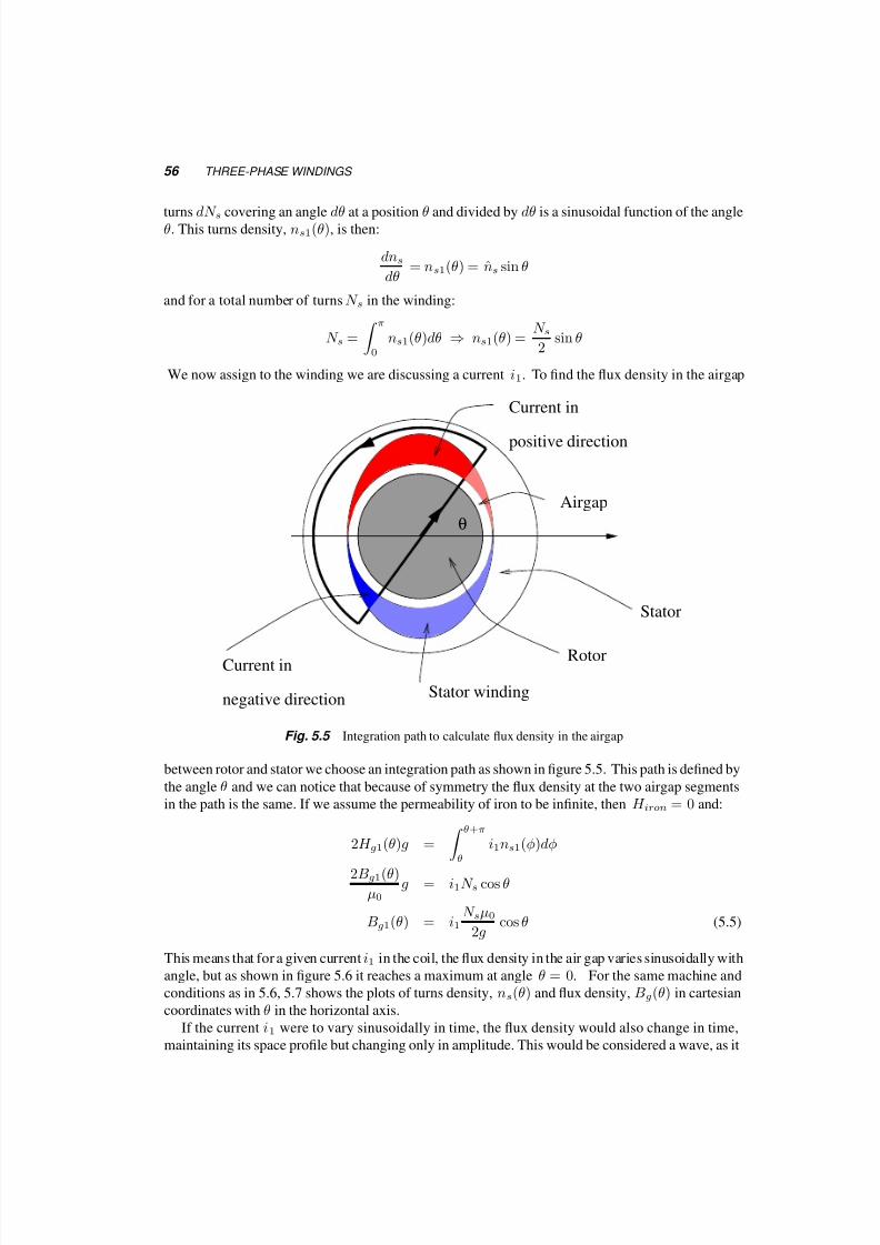
5/17/2018 Electrical Machines and Drives - slidepdf.com
http://slidepdf.com/reader/full/electrical-machines-and-drives-55ab59315f602 64/123
56 THREE-PHASE WINDINGS
turns dN s covering an angle dθ at a position θ and divided by dθ is a sinusoidal function of the angleθ. This turns density, ns1(θ), is then:
dns
dθ= ns1(θ) = ns sin θ
and for a total number of turns N s in the winding:
N s =
π
0
ns1(θ)dθ ⇒ ns1(θ) =N s2
sin θ
We now assign to the winding we are discussing a current i1. To find the flux density in the airgap
negative direction
Current in
θ
Rotor
Airgap
positive direction
Current in
Stator
Stator winding
Fig. 5.5 Integration path to calculate flux density in the airgap
between rotor and stator we choose an integration path as shown in figure 5.5. This path is defined by
the angle θ and we can notice that because of symmetry the flux density at the two airgap segments
in the path is the same. If we assume the permeability of iron to be infinite, then H iron = 0 and:
2H g1(θ)g = θ+π
θ
i1ns1(φ)dφ
2Bg1(θ)
µ0g = i1N s cos θ
Bg1(θ) = i1N sµ0
2gcos θ (5.5)
This means that for a given current i1 in the coil, the flux density in the air gap varies sinusoidally with
angle, but as shown in figure 5.6 it reaches a maximum at angle θ = 0. For the same machine and
conditions as in 5.6, 5.7 shows the plots of turns density, ns(θ) and flux density, Bg(θ) in cartesian
coordinates with θ in the horizontal axis.
If the current i1 were to vary sinusoidally in time, the flux density would also change in time,
maintaining its space profile but changing only in amplitude. This would be considered a wave, as it

5/17/2018 Electrical Machines and Drives - slidepdf.com
http://slidepdf.com/reader/full/electrical-machines-and-drives-55ab59315f602 65/123
STATOR WINDINGS AND RESULTING FLUX DENSITY 57
Fig. 5.6 Sketch of the flux in the airgap
0 90 180 270 360−1
0
1
n s
( θ )
0 90 180 270 360−1
0
1
θ
B g
( θ )
Fig. 5.7 Turns density on the stator and air gap flux density vs. θ
changes in time and space. The nodes of the wave, where the flux density is zero, will remain at 900
and 2700, while the extrema of the flux will remain at 00 and 1800.
Consider now an additional winding, identical to the first, but rotated with respect to it by 1200.
For a current in this winding we’ll get a similar airgap flux density as before, but with nodes at
900 +1200 and at 2700 +1200. If a current i2 is flowing in this winding, then the airgap flux density

5/17/2018 Electrical Machines and Drives - slidepdf.com
http://slidepdf.com/reader/full/electrical-machines-and-drives-55ab59315f602 66/123
58 THREE-PHASE WINDINGS
due to it will follow a form similar to equation 5.5 but rotated 1200
=2π
3 .
Bg2(θ) = i2N sµ0
2gcos(θ − 2π
3) (5.6)
Similarly, a third winding, rotated yet another 1200 and carrying current i3, will produce airgap
flux density:
Bg3(θ) = i3N sµ0
2gcos(θ − 4π
3) (5.7)
Superimposing these three flux densities, we get yet another sinusoidally distributed airgap flux
density, that could equivalently come from a winding placed at an angle φ and carrying current i:
Bg(θ) = Bg1(θ) + Bg2(θ) + Bg3(θ) = iN sµ0
2gcos(θ + φ) (5.8)
This means that as the currents change, the flux could be due instead to only one sinusoidally
distributed winding with the same number of turns. The location, φ(t), and current, i(t), of this
winding can be determined from the current space vector:
i(t) = i(t)φ(t) = i1(t) + i2(t)ej1200 + i3(t)ej2400
5.2.1 Balanced, Symmetric Three-phase Currents
If the currents i1, i2, i3 form a balanced three-phase system of frequency f s = ωs/2π, then we can
write:
i1 = √2I cos(ωst + φ1) = √22
Isejωst + Ise−jωst
i2 =√
2I cos(ωst − φ1 +2π
3) =
√2
2
Isej(ωst−2π/3) + Ise−j(ωst−2π/3)
(5.9)
i3 =√
2I cos(ωst − φ1 +4π
3) =
√2
2
Isej(ωst−4π/3) + Ise−j(ωst−4π/3)
where I is the phasor corresponding to the current in phase 1. The resultant space vector is
is(t) =3
2
√2
2Iejωst =
3
2
√2
2Iej(ωst+φ1) I = Iej(φ1+
π2) (5.10)
The resulting flux density wave is then:
B(θ, t) =3
2
√2I
N sµ0
2gcos(ωst + φ1 − θ) (5.11)
which shows a travelling wave, with a maximum value B = 32
√2I N s
µ0
. This wave travels around the
stator at a constant speed ωs, as shown in figure 5.8
5.3 PHASORS AND SPACE VECTORS
It is easy at this point to confuse space vectors and phasors. A current phasor, I = Iejφ0 , describes
one sinusoidally varying current, of frequency ω, amplitude√
2I and initial phase φ0. We can
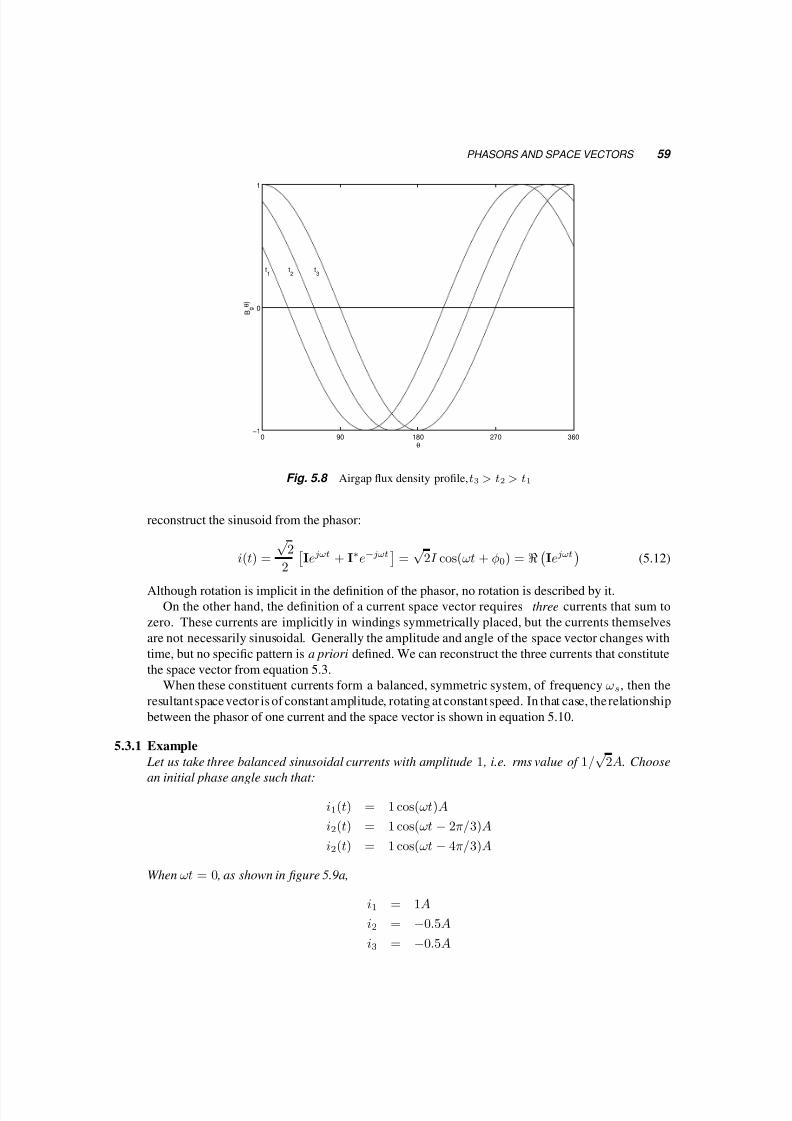
5/17/2018 Electrical Machines and Drives - slidepdf.com
http://slidepdf.com/reader/full/electrical-machines-and-drives-55ab59315f602 67/123
PHASORS AND SPACE VECTORS 59
0 90 180 270 360−1
0
1
θ
B g
θ )
t1
t2
t3
Fig. 5.8 Airgap flux density profile, t3 > t2 > t1
reconstruct the sinusoid from the phasor:
i(t) =
√2
2 Iejωt + I∗e−jωt
=
√2I cos(ωt + φ0) =
Iejωt
(5.12)
Although rotation is implicit in the definition of the phasor, no rotation is described by it.
On the other hand, the definition of a current space vector requires three currents that sum to
zero. These currents are implicitly in windings symmetrically placed, but the currents themselves
are not necessarily sinusoidal. Generally the amplitude and angle of the space vector changes with
time, but no specific pattern is a priori defined. We can reconstruct the three currents that constitute
the space vector from equation 5.3.
When these constituent currents form a balanced, symmetric system, of frequency ωs, then the
resultant space vector is of constant amplitude, rotating at constant speed. In that case, the relationship
between the phasor of one current and the space vector is shown in equation 5.10.
5.3.1 Example
Let us take three balanced sinusoidal currents with amplitude 1 , i.e. rms value of 1/√
2A. Choose
an initial phase angle such that:
i1(t) = 1 cos(ωt)A
i2(t) = 1 cos(ωt − 2π/3)A
i2(t) = 1 cos(ωt − 4π/3)A
When ωt = 0 , as shown in figure 5.9a,
i1 = 1A
i2 = −0.5A
i3 = −0.5A

5/17/2018 Electrical Machines and Drives - slidepdf.com
http://slidepdf.com/reader/full/electrical-machines-and-drives-55ab59315f602 68/123
60 THREE-PHASE WINDINGS
i = i1 + i2ej1200
+ i3ej2400
= 1.5
0
Aand later, when ωt = 200 = π/9 rad , as shown in figure 5.9b,
i1 = 0.939A
i2 = −0.766A
i3 = −0.174A
i = i1 + i2ej1200 + i3ej2400 = 1.5 200A
i
i3
= -0.5A
i2
= -0.5A
i1
= 1A
_
(a)
=-0.1737A3
i
i
_
i2
= -0.766A
1i = 0.9397A
(b)
Fig. 5.9 Space vector movement for sinusoidal, symmetric three-phase currents
5.4 MAGNETIZING CURRENT, FLUX AND VOLTAGE
Let us now see what results this rotating flux has on the windings, using Faraday’s law. From this
point on we’ll use sinusoidal symmetric three-phase quantities.
We look again at our three real stationary windings linked by a rotating flux. For example, when
the current is maximum in phase 1, the flux is as shown in figure 5.10a, linking all of the turns in
phase 1. Later, the flux has rotated as shown in figure 5.10b, resulting in lower flux linkages with
the phase 1 windings. When the flux has rotated 900, as in 5.10c the flux linkages with the phase 1
winding are zero.
To calculate the flux linkages λ we have to take a turn of the winding, placed at angle θ, as shown
in figure 5.11. The flux through this coil is:
Φ(t, θ) =
θ
θ−π
Bg(t, φ)dA = lr
θ+
θ−π
Bg(t, φ)dφ (5.13)
But the number of turns linked by this flux is dns(θ) = ns(θ)dθ, so the flux linkages for these turns
are:
dλ = ns(θ)dθ · Φ(θ)

5/17/2018 Electrical Machines and Drives - slidepdf.com
http://slidepdf.com/reader/full/electrical-machines-and-drives-55ab59315f602 69/123
MAGNETIZING CURRENT, FLUX AND VOLTAGE 61
(a) (b) (c)
Fig. 5.10 Rotating flux and flux linkages with phase 1
Fig. 5.11 Flux linkages of one turn
To find the flux linkages λ1 for all of the coil, we have to integrate the flux linkages over all turns of
coil 1:
λ1 =
π
0
λ(θ)dθ
giving us at the end:
λ1(t) =N 2s lr
8g3πµ0
√2I cos(ωt + φ1) = LM
√2I cos(ωt + φ1) (5.14)
which means that the flux linkages in coil 1 are in phase with the current in this coil and proportional
to it. The flux linkages of the other two coils, 2 and 3, are identical to that of coil 1, and lagging in
time by 1200 and 2400. With these three quantities we can create a flux-linkage space vector, λλλ.
λλλ ≡ λ1 + λ2ej1200 + λ3ej2400 = LM i (5.15)
Since the flux linkages of each coil vary, and in our case sinusoidally, a voltage is induced in each
of these coils. The induced voltage in each coil is 900 ahead of the current in it, bringing to mind

5/17/2018 Electrical Machines and Drives - slidepdf.com
http://slidepdf.com/reader/full/electrical-machines-and-drives-55ab59315f602 70/123
62 THREE-PHASE WINDINGS
the relationship of current and voltage of an inductor. Notice though, that it is not just the current inthe winding that causes the flux linkages and the induced voltages, but rather the current in all three
windings. Still, we call the constant LM magnetizing inductance.
e1(t) =dλ1dt
= ω√
2I cos(ωt + φ1 +π
2)
e2(t) =dλ2dt
= ω√
2I cos(ωt + φ1 +π
2− 2π
3) (5.16)
e3(t) =dλ3dt
= ω√
2I cos(ωt + φ1 +π
2− 4π
2)
and of course we can define voltage space vectors e:
e = e1 + e2ej1200
+ e3ej2400
= jωLM i (5.17)
Note that the flux linkage space vector λλλ is aligned with the current space vector, while the voltage
space vector e is ahead of both by 900. This agrees with the fact that the individual phase voltages
lead the currents by 900, as shown in figure 5.12.
i
ωt
e
λ
Fig. 5.12 Magnetizing current, flux-linkage and induced voltage space vectors

5/17/2018 Electrical Machines and Drives - slidepdf.com
http://slidepdf.com/reader/full/electrical-machines-and-drives-55ab59315f602 71/123
6 Induction Machines
Induction machines are often described as the ‘workhorse of industry’. This clice reflects the reality
of the qualities of these machines. They are cheap to manufacture, rugged and reliable and find their
way in most possible applications. Variable speed drives require inexpensive power electronics and
computer hardware, and allowed induction machines to become more versatile. In particular, vector
or field-oriented control allows induction motors to replace DC motors in many applications
6.1 DESCRIPTION
The stator of an induction machine is a typical three-phase one, as described in the previous chapter.
The rotor can be one of two major types. Either a) it is wound in a fashion similar to that of the stator
with the terminals led to slip rings on the shaft, as shown in figure 6.1, or b) it is made with shorted
Shaft
Rings
Rotor
Slip
Fig. 6.1 Wound rotor slip rings and connections
bars. Figure 6.2 shows the rotor of such a machine, while figures 6.3 show the shorted bars and the
laminations.
The picture of the rotor bars is not easy to obtain, since the bars are formed by casting aluminum
in the openings of the rotor laminations. In this case the iron laminations were chemically removed.
63

5/17/2018 Electrical Machines and Drives - slidepdf.com
http://slidepdf.com/reader/full/electrical-machines-and-drives-55ab59315f602 72/123
64 INDUCTION MACHINES
Fig. 6.2 Rotor for squirrel cage induction motor
(a) Rotor bars and rings (b) Rotor
Fig. 6.3 Rotor Components of a Squirrel Cage Induction Motor
6.2 CONCEPT OF OPERATION
As these rotor windings or bars rotate within the magnetic field created by the stator magnetizing
currents, voltages are induced in them. If the rotor were to stand still, then the induced voltages
would be very similar to those induced in the stator windings. In the case of squirrel cage rotor, the
voltage induced in the bars will be slightly out of phase with the voltage in the next one, since the
flux linkages will change in it after a short delay.
If the rotor is moving at synchronous speed, together with the field, no voltage will be induced in
the bars or the windings.

5/17/2018 Electrical Machines and Drives - slidepdf.com
http://slidepdf.com/reader/full/electrical-machines-and-drives-55ab59315f602 73/123
CONCEPT OF OPERATION 65
B g
1
2
3
4
567
13
19
(a) Rotor bars in the stator field
0 90 180 270 360−1
0
1
t
e ( t )
bar 1
bar 2
bar 3
bar 7
(b) Voltages in rotor bars
Fig. 6.4
Generally when the synchronous speed is ωs = 2πf s, and the rotor speed ω0, the frequency of
the induced voltages will be f r, where 2πf r = ωs − ω0. Maxwell’s equation becomes here:
−→E = −→v × −→Bg (6.1)
where −→v is the relative velocity of the rotor with respect to the field:
v = (ωs − ω0)r (6.2)
Since a voltage is induced in the bars, and these are short-circuited, currents will flow in them. The
current density−→J (θ) will be:
−→J (θ) =
1
ρ
−→E (6.3)
These currents are out of phase in different bars, just like the induced voltages. To simplify the
analysis we can consider the rotor as one winding carrying currents sinusoidally distributed in space.
This will be clearly the case for a wound rotor. It will also be the case for uniformly distributed rotor
bars, but now each bar, located at an angle θ will carry different current, as shown in figure 6.5 a:
J =1
ρ(ωs − ω0) · Bg(θ) (6.4)
J (θ) =1
ρ(ωs − ω0)Bg sin(θ) (6.5)
We can replace the bars with a conductive cylinder as shown in figure 6.5 b.
We define as slip s the ratio:
s =ωs − ω0
ωs(6.6)

5/17/2018 Electrical Machines and Drives - slidepdf.com
http://slidepdf.com/reader/full/electrical-machines-and-drives-55ab59315f602 74/123
66 INDUCTION MACHINES
B g
++
+
+
+
+
+
++
+
+
(a) Currents in rotor bars
B g
++
+
+
+
+
+
++
+
+
Equivalent
Conducting
Sheet
(b) Equivalent Current Sheet in Rotor
Fig. 6.5 Current Distribution in equivalent conducting sheet
At starting the speed is zero, hence s = 1, and at synchronous speed, ωs = ω0, hence s = 0. Above
synchronous speed s < 0, and when the rotor rotates in a direction opposite of the magnetic field
s > 1.
6.2.1 Example
The rotor of a two-pole 3-phase induction machine rotates at 3300rpm, while the stator is fed by athree-phase system of voltages, at 60Hz. What are the possible frequencies of the rotor voltages?
At 3300 rpm
ωo = 33002π
60= 345.6rad/s while ωs = 377rad/s
These two speeds can be in the opposite or the same direction, hence:
ωr = ωs − ωo = 377 ± 345.6 = 722.58rad/s or 31.43rad/s
f r = 115Hz or = 5Hz
6.3 TORQUE DEVELOPMENT
We can now calculate forces and torque on the rotor. We’ll use the formulae:
F = Bli, T = F · r (6.7)
since the flux density is perpendicular to the current. As l we’ll use the length of the conductor, i.e.
the depth of the motor. We consider an equivalent thickness of the conducting sheet de. A is the
cross section of all the bars.
A = nrotor barsπ
4d2 = 2πrde (6.8)
de =nrotor barsd2
8r(6.9)

5/17/2018 Electrical Machines and Drives - slidepdf.com
http://slidepdf.com/reader/full/electrical-machines-and-drives-55ab59315f602 75/123
OPERATION OF THE INDUCTION MACHINE NEAR SYNCHRONOUS SPEED 67
(b)(a
θ
θ
r
d
d
ed
Fig. 6.6 Calculation of Torque
For a small angle dθ at an angle θ, we calculate the contribution to the total force and torque:
dF = (JdA) · Bg · l, Bg = Bg sin(θ)
dF = (Jder dθ)Bg
dT = r dF
T =
θ=2π
θ=0
dT =
2πr2lde
ρ
B2
g (ωs − ω0) (6.10)
Flux density in the airgap is not an easy quantity to work with, so we can use the relationship
between flux density (or flux linkages) and rotor voltage and finally get:
T =
8
π
rde
N 2s ρl
Λ2
s(ωs − ω0) where Λs =
E sωs
(6.11)
Although the constants in equations 6.10 and 6.11 are important we should focus more on the
variables. We notice that in equation 6.10 the torque is proportional to the frequency of the rotor
currents, (ωs − ω0) and the square of the flux density. This is so since the torque comes from the
interaction of the flux density Bg and the rotor currents. But the rotor currents are induced ( induction
motor) due to the flux Bg and the relative speed ωs − ω0.
On the other hand, equation 6.11 gives us torque as a function of more accessible quantities, stator
induced voltage E s and frequency ωs. This is so, since there is a very simple and direct relationship
between stator induced voltage, flux (or flux linkages) and frequency.
6.4 OPERATION OF THE INDUCTION MACHINE NEAR SYNCHRONOUS SPEED
We already determined that the voltages induced in the rotor bars are of slip frequency, f r =(ωs − ω0)/(2π). At rotor speeds near synchronous, this frequency, f r is quite small. The rotor bars
in a squirrel cage machine possess resistance and leakage inductance, but at very low frequencies,

5/17/2018 Electrical Machines and Drives - slidepdf.com
http://slidepdf.com/reader/full/electrical-machines-and-drives-55ab59315f602 76/123
68 INDUCTION MACHINES
i.e near synchronous speed, we can neglect this inductance. The rotor currents therefore are limitednear synchronous speed by the rotor resistance only.
The induced rotor-bar voltages and currents form space vectors. These are perpendicular to the
stator magnetizing current and in phase with the space vectors of the voltages induced in the stator
as shown in figure 6.7 and figure
+
+ +
+ +
+
+ +
+++
+
+
+
++
+
++
i r
i s,m
B g
+ +
+
Fig. 6.7 Stator Magnetizing Current, airgap flux and rotor currents
Theserotor currents, ir produce additional airgapflux, which is 900 outof phase of the magnetizing
flux. But the stator voltage, es, is applied externally and it is proportional to and 900 out of phase of
the airgap flux. Additional currents, isr will flow in the stator windings in order to cancel the flux
due to the rotor currents. These currents are shown in figures 6.8. In 6.9 the corresponding space
vectors are shown.
+
+
+
+
+
+
+
+
+
+
+
+ +
+
+ +
+ +
++ +
B
++
+
+
+
+
+
+
+
++
g
s,m
+
i
i s,r
i r
(a) Rotor Current and Stator Current Components
++
+
+ +
++
B
i
+
+
+
+
+
+ +
+ + +
+
+
+
+
+
s
g
i s
(b) Space Vectors of the Rotor and Stator Cur-
rents and induced voltages
Fig. 6.8 Rotor and Stator Currents in an Induction Motor
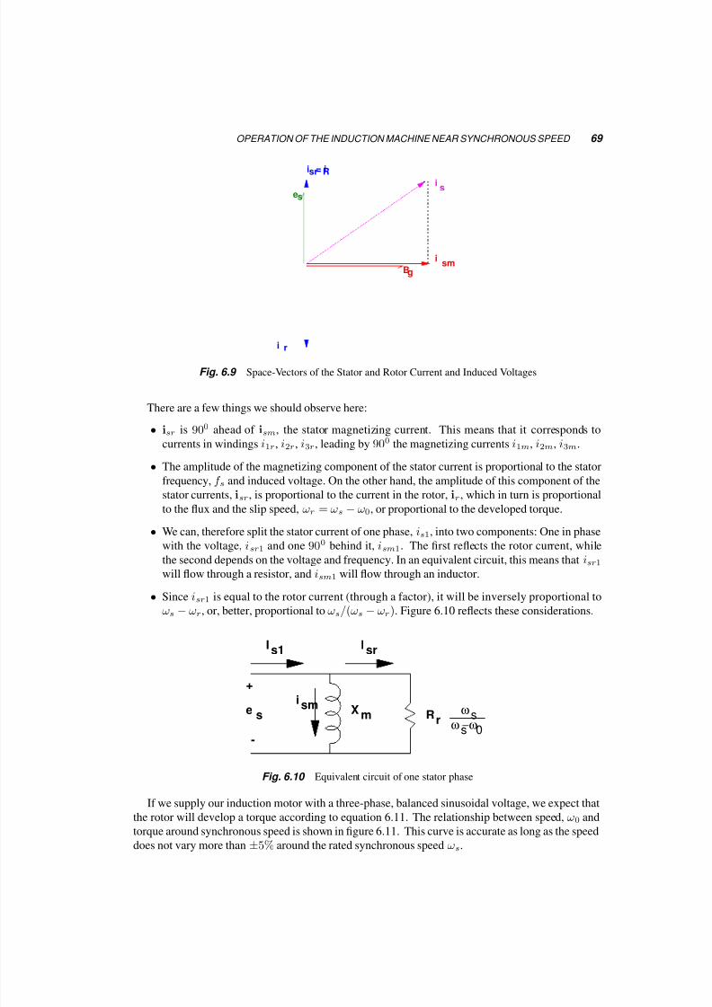
5/17/2018 Electrical Machines and Drives - slidepdf.com
http://slidepdf.com/reader/full/electrical-machines-and-drives-55ab59315f602 77/123
OPERATION OF THE INDUCTION MACHINE NEAR SYNCHRONOUS SPEED 69
es
R= i
sr
i
i
gB
si
sm
ri
Fig. 6.9 Space-Vectors of the Stator and Rotor Current and Induced Voltages
There are a few things we should observe here:
• isr is 900 ahead of ism, the stator magnetizing current. This means that it corresponds to
currents in windings i1r, i2r, i3r, leading by 900 the magnetizing currents i1m, i2m, i3m.
• The amplitude of the magnetizing component of the stator current is proportional to the stator
frequency, f s and induced voltage. On the other hand, the amplitude of this component of the
stator currents, isr, is proportional to the current in the rotor, ir , which in turn is proportional
to the flux and the slip speed, ωr = ωs − ω0, or proportional to the developed torque.
• We can, therefore split the stator current of one phase, is1, into two components: One in phase
with the voltage, isr1 and one 900 behind it, ism1. The first reflects the rotor current, while
the second depends on the voltage and frequency. In an equivalent circuit, this means that isr1
will flow through a resistor, and ism1 will flow through an inductor.
• Since isr1 is equal to the rotor current (through a factor), it will be inversely proportional to
ωs − ωr, or, better, proportional to ωs/(ωs − ωr). Figure 6.10 reflects these considerations.
I
i
Isr
smX
m Rr
s1
0ω −ωs
ωs
+
es
-
Fig. 6.10 Equivalent circuit of one stator phase
If we supply our induction motor with a three-phase, balanced sinusoidal voltage, we expect that
the rotor will develop a torque according to equation 6.11. The relationship between speed, ω0 and
torque around synchronous speed is shown in figure 6.11. This curve is accurate as long as the speed
does not vary more than ±5% around the rated synchronous speed ωs.

5/17/2018 Electrical Machines and Drives - slidepdf.com
http://slidepdf.com/reader/full/electrical-machines-and-drives-55ab59315f602 78/123
70 INDUCTION MACHINES
T
ω0
ωs
Fig. 6.11 Torque-speed characteristic near synchronous speed
We notice in 6.11 that when the speed exceeds synchronous, the torque produced by the machine
is of opposite direction than the speed, i.e. the machine operates as a generator, developing a torqueopposite to the rotation (counter torque) and transferring power from the shaft to the electrical system.
We already know the relationship of the magnetizing current, I sm to the induced voltage E sm
through our analysis of the three-phase windings. Let us now relate the currents ir and isr with the
same induced voltage.
The current density on the rotor conducting sheet−→J is related to the value of the airgap flux
density−→B g through:
−→J =
1
ρ(ωs − ω0)
−→B g (6.12)
This current density corresponds to a space vector ir that is opposite to the isr in the stator. This
current space vector will correspond to the same current density:
J = isrN s 1r d
(6.13)
while the stator voltage es is also related to the flux density Bg. Its amplitude is:
es = ωsπ
2N slrBg (6.14)
Finally, substituting into 6.12, and relating phasors instead of space vectors, we obtain:
Es = RRωs
ωs − ωoIsr (6.15)
Using this formulation we arrive at the formula for the torque:
T = 3
E 2s
ωs
1
RR
ωs
−ω0
ωs = 3
Λ2s
RR ωr =
3P g
ωs (6.16)
Here P g is the power transferred to the resistance RRωs
ωs−ω0
, through the airgap. Of this power
a portion is converted to mechanical power represented by losses on resistance RRω0
ωs−ω0
, and the
remaining is losses in the rotor resistance, represented by the losses on resistance RR. Figure
6.12 shows this split in the equivalent circuit. Note that the resistance RRω0
ωs−ω0
can be negative,
indicating that mechanical power is absorbed in the induction machine.
6.4.1 Example
A 2-pole three-phase induction motor is connected in Y and is fed from a 60Hz , 208V (l − l) system.
Its equivalent one-phase rotor resistance is RR = 0.1125Ω. At what speed and slip is the developed
torque 28N m?

5/17/2018 Electrical Machines and Drives - slidepdf.com
http://slidepdf.com/reader/full/electrical-machines-and-drives-55ab59315f602 79/123
LEAKAGE INDUCTANCES AND THEIR EFFECTS 71
0ω
sω −ω
0R
R
RR
s1
mX
sm
sr
I
i
I
0ω −ωs
ωsR
R
Fig. 6.12 Equivalent circuit of one stator phase separating the loss and torque rotor components
srI
s1I
Xlrls
s
sV
-
+
sE
-
+
0ω −ωs
ωsR
R
RX
0ω
sω −ω
0
ism
Xm
R
RR
R
Fig. 6.13 Complete equivalent circuit of one stator phase
T = 3
V sωs
21
RRωr with V s = 120V
28 = 3
120
377
21
0.1125ωr ⇒ ωr = 10.364
s =ωr
ωs=
10.364a
377= 0.0275
ωo = ωs − ωr = 366.6rad/s
6.5 LEAKAGE INDUCTANCES AND THEIR EFFECTS
In the previous discussion we assumed that all the flux crosses the airgap and links both the statorand rotor windings. In addition to this flux there are flux components which link only the stator or
the rotor windings and are proportional to the currents there, producing voltages in these windings
900 ahead of the stator and rotor currents and proportional to the amplitude of these currents and
their frequency.
This is simple to model for the stator windings, since the equivalent circuit we are using is of the
stator, and we can model the effects of this flux with only an inductance. The rotor leakage flux can
be modelled in the rotor circuit with an inductance Lls, as well, but corresponding to frequency of
f r = ωs−ω0
2π, the frequency of the rotor currents. It turns out that when we try to see its effects on
the stator we can model it with an inductance Llr at frequency f s, as shown in the complete 1-phase
equivalent circuit in figure 6.13.

5/17/2018 Electrical Machines and Drives - slidepdf.com
http://slidepdf.com/reader/full/electrical-machines-and-drives-55ab59315f602 80/123
72 INDUCTION MACHINES
Here Es is the phasor of the voltage induced into the rotor windings from the airgap flux, whileVs is the phasor of the applied 1-phase stator voltage. The torque equations discussed earlier, 6.16,
still hold, but give us slightly different results: We can develop torque-speed curves, by selecting
speeds, solving the equivalent circuit, calculating power P g, and using equation 6.16 for the torque.
Figure 6.14 shows these characteristics for a wide range of speeds.
I
s
T
ω
p f
ωs
ωmaxT
ωN
0
Fig. 6.14 Torque, current and power factor of an induction motor vs. speed
6.6 OPERATING CHARACTERISTICS
Figure 6.14 shows the developed torque, current, and power factor of an induction motor over a
speed range from below zero (slip > 1) to above synchronous (slip < 0). It is clear that there are
three areas of interest:
1. For speed 0 ≤ ωo ≤ ωs the torque is of the same sign as the speed, and the machine operates
as a motor. There are a few interesting point on this curve, and on the corresponding current
and p.f. curves.
2. For speed ω0 ≤ 0, torque and speed have opposite signs, and the machine is in breaking mode.
Notice that the current is very high, resulting in high winding losses.
3. for speed ωs ≥ ωs the speed and torque are of opposite signs, the machine is in generating
mode, and the current amplitude is reasonable.
Let us concentrate now on the region 0 ≤ ωo ≤ ωs. The machine is often designed to operate as
a motor, and the operating point is near or exactly where the power factor is maximized. It is for this

5/17/2018 Electrical Machines and Drives - slidepdf.com
http://slidepdf.com/reader/full/electrical-machines-and-drives-55ab59315f602 81/123
OPERATING CHARACTERISTICS 73
lrXR Th XTh
sω
sω −ω
0R
RTh srV
−
+
I
0ω
sω −ω
0R
R
RR
Fig. 6.15 Equivalent circuit of the stator with Thevenin equivalent of the stator components
point that the motor characteristics are given on the nameplate, rated speed, current, power factorand torque. When designing an application it is this point that we have to consider primarily: Will
the torque suffice, will the efficiency and power factor be acceptable?
A second point of interest is starting, ( slip s = 1) where the torque is not necessarily high,
but the current often is. When selecting a motor for an application, we have to make sure that this
starting torqueis adequate to overcomethe load torque, which mayalso include a static component. In
addition, thestartingcurrent is often 3-5timesthe rated current of themachine. If thedeveloped torque
at starting is not adequately higher than the load starting torque, their difference, the accelerating
torque will be small and it may take too long to reach the operating point. This means that the current
will remain high for a long time, and fuses or circuit breakers may operate.
A third point of interest is the maximum torque, T max, corresponding to speed ωTmax. We can
find it by analytically calculating torque as a function of slip, and equating the derivative to 0. This
point is interesting, since points to the right of it correspond in general to stable operating conditions,
while point to its left correspond to unstable operating conditions.We can study this point if we take the Thevenin equivalent circuit of the left part of the stator
equivalent circuit, including, V s, Rs, X ls and X m. This will give us the circuit in figure 6.15.
Using the formula 6.16 we arrive at:
T = 31
ωs
V 2T h
RR
s
RT h + RR
s
2+ (X T h + X lr)
2(6.17)
The maximum torque will develop when the airgap power, P g, i.e. the power delivered to RR/s,
is maximum, since the torque is proportional to it. Taking derivative of 6.17, we find that maximum
torque will occur when:
RR
smaxT =
(RT h)
2+ (X T h + X lr)
2or (6.18)
smaxT =RR
R2T h + (X T h + X lr)2
(6.19)
giving maximum torque:
T max = 31
2ωs
V 2T h
RT h +
R2T h + (X T h + X lr)2
(6.20)

5/17/2018 Electrical Machines and Drives - slidepdf.com
http://slidepdf.com/reader/full/electrical-machines-and-drives-55ab59315f602 82/123
74 INDUCTION MACHINES
ω
T
RR=r
1RR=2*r
1
ω
I
RR=r
1
RR=2*r
1
Fig. 6.16 Effect of changing rotor resistance on the torque-speed and current speed characteristic
If we neglect the stator resistance we can easily show that the general formula for the torque
becomes:
T = T max2
s
sTmax
+ sTmax
s
(6.21)
If we neglect both the stator resistance and the magnetizing inductance, we can develop simple
formulae for T max and ωTmax. To do so we have to assume operation near synchronous speed,
where that value of RRωs
ωs−ωois much larger than ωsLlr .
ωTmax = ωs − RR
Llr + Lls(6.22)
T max 3
2
V sωs
21
RR(ωs − ωTmax) =
3
2
V sωs
21
Lls + Llr(6.23)
We notice here that the slip frequency at this torque, ωr = ωs
−ωTmax, for a constant flux
Λs = Esωs is independent of frequency and proportional to the resistance RR. We already know
that this resistance is proportional to the rotor resistance, so if the rotor resistance is increased, the
torque-speed characteristic is shifted to the left, as shown in figure 6.16.
If we have convenient ways to increase the rotor resistance, we can increase the starting torque,
while decreasing the starting current. Increasing the rotor resistance can be easily accomplished in a
wound-rotor machine, and more complex in squirrel cage motor, by using double or deep rotor bars.
In the formulae developed we notice that the maximum torque is a function of the flux. This
means that we can change the frequency of the stator voltage, but as long as the voltage amplitude
changes so that the flux stays the same, the maximum torque will also stay the same. Figure 6.17
shows this. This is called Constant Volts per Hertz Operation and it is a first approach to controlling
the speed of the motor through its supply.

5/17/2018 Electrical Machines and Drives - slidepdf.com
http://slidepdf.com/reader/full/electrical-machines-and-drives-55ab59315f602 83/123
STARTING OF INDUCTION MOTORS 75
ω
T
fs=50Hz
fs=35Hz
fs=20Hz
load
ω
I
s
Fig. 6.17 Effect on the Torque - Speed characteristic of changing frequency while keeping flux constant
Near synchronous speed the effect of the rotor leakage inductance can be neglected, as discussed
earlier. This assumption gives us the approximate torque-speed equation 6.16 discussed earlier.
T = 3E 2sωs
1
RR
ωs − ω0
ωs= 3
Λ2sωr
RR=
3P gωs
Figure 6.18 shows both exact and approximate torque-speed characteristics. It is important to notice
that the torque calculated from the approximate equation is grossly incorrect away from synchronous
speed.
6.7 STARTING OF INDUCTION MOTORS
To avoid the problems associated with starting (too high current, too low torque), a variety of
techniques are available.
An easy way to decrease the starting current is to decrease the stator terminal voltage. One can
notice that while the stator current is proportional to the in voltage, torque will be proportional to
its square. If a transformer is used to accomplish this, both developed torque and line current will
decrease by the square of the turns ratio of the transformer.A commonly used method is to use a motor designed to operate with the stator windings connected
in ∆, and have it connected in Y at starting. As the voltage ratio is.
V s,Y =1√
3V s,∆ (6.24)
then
I s,Y =1√
3I s,∆ (6.25)
T s,Y =1
3T s,∆ (6.26)

5/17/2018 Electrical Machines and Drives - slidepdf.com
http://slidepdf.com/reader/full/electrical-machines-and-drives-55ab59315f602 84/123
76 INDUCTION MACHINES
ω
T
ωs
0 ωmaxT
Fig. 6.18 Exact and approximate torque-speed characteristics
-
V∆
+I
sYV+
ll
V
-
ll
I line,Y
sY
s
s-
+V
I
I
∆
∆line+
Fig. 6.19 Y - Delta starting of an induction motor
But in a ∆ connection, I line =√
3I ph, leading to:
I line,Y =1
3I line,∆ (6.27)
Once the machine has approached the desired operating point, we can reconfigure the connection
to ∆, and provide better efficiency.
This decrease in current is often adequate to allow a motor to start at low load starting torque.Using a variable frequency and voltage supply we could comfortable increase the starting torque, as
shown in figure 6.17, while decreasing the starting current.
6.8 MULTIPLE POLE PAIRS
If we considerthat an induction machine will operate close to synchronous speed (3000rpm for 50Hzand 3600rpm for 60Hz) we may find that the speed of the machine is too high for an application.
If we recall the pictures of the flux in AC machines we have seen, we can notice that the flux has a
relatively long path to travel in the stator making the stator heavy and lossy.

5/17/2018 Electrical Machines and Drives - slidepdf.com
http://slidepdf.com/reader/full/electrical-machines-and-drives-55ab59315f602 85/123
MULTIPLE POLE PAIRS 77
Fig. 6.20 Equivalent windings for a 6 pole induction motor
A machine with more than one pole pair is quite similar to that with only one. The difference is
that for example in a 4 pole machine each side of a sinusoidally distributed winding of one phase
covers only 900 instead of 1800. A result is that there is room for four rather than two coil sides of
each phase. Figure 6.20 shows at one instant the equivalent windings resulting from the the three
phase windings.
The effects of a large number of poles on the operation of the machine are easy to predict. If the
machine has p poles, or p/2 pairs of poles, in one period of the voltage the flux will travel 2 p ws rad/s.
Hence the rotor speed corresponding to synchronous will be ωsm:
ωsm = 2 p
ωs (6.28)
We introduce now the actual, mechanical speed of the rotor, ωm, while we keep the term ωo as
the rotor speed of a two pole motor. We generally measure ωm in rad/s, while we measure ω0 in
electrical rad/s. We retain the same definition for slip based on the electrical speed ω0 .
ωm =2
pωo (6.29)
s =ωs − ω0
ωs=
ωs − p2ωm
ωs(6.30)
This means that for a 4 pole machine, supplied from a source of at 60Hz, and operating close to
rated conditions, the speed will be near 1800rpm, while for a 6 pole machine, the speed will be near1200rpm.
While increasing the number of poles results in a decrease of the synchronous and operating
speeds of the machine, it also results in an increase of the developed torque of the machine by the
same ratio. Hence, the corrected torque formula will be
T = 3 p
2
P gωs
= 3 p
2
P mω0
(6.31)
Similarly, the torque near the synchronous speed is:
T = 3 p
2
E 2sωs
1
RR
ωs − ω0
ωs= 3
p
2
Λ2sωr
RR= 3
p
2
P gωs

5/17/2018 Electrical Machines and Drives - slidepdf.com
http://slidepdf.com/reader/full/electrical-machines-and-drives-55ab59315f602 86/123
78 INDUCTION MACHINES
while the previously developed formulas for maximum torque will become:
T max = 3 p
2
1
2ωs
V 2T h
RT h +
R2T h + (X T h + X lr)
2(6.32)
and
T max 3
2
p
2
V sωs
21
RR(ωs − ωTmax) =
3
2
p
2
V sωs
21
Lls + Llr(6.33)
6.8.1 Example
A 3-phase 2-pole induction motor is rated 190V , 60Hz , it is connected in Y , and has Rr = 6.6Ω ,
Rs = 3.1Ω , X M = 190Ω , X lr = 10Ω , and X ls = 3Ω. Calculate the motor starting torque, starting
current and starting power factor under rated voltage. What will be the current and power factor if
no load is connected to the shaft?
1. At starting s = 1:
Is =190√
3/ [3.1 + j3] + j190||(6.6 + j10) = 7.06
−54.50A
IR = Is j190
6.6 + j10 + j190= 6.7
−52.60A
T = 3P gap
ωs
p
2= 3
6.72 · 6.6
377
2
2= 2.36N m
2. Under no load the speed is synchronous and s = 0:
Is = 110/ [3.1 + j3 + j190] = 0.57−89.10
AI s = 0.57A
pf = 0.016lagging
6.8.2 Example
A 3-phase 2-pole induction motor is rated 190V , 60Hz it is connected in Y , and has Rr = 6.6Ω ,
Rs = 3.1Ω , X M = 190Ω , X lr = 10Ω , and X ls = 3Ω. It is operating from a variable speed -
variable frequency source at a speed of 1910rpm, under a constant V /f policy and the developed
torque is 0.8N m. What is the voltage and frequency of the source? (Hint: Calculate first the slip).
The ratio V s/ωs stays 110/377.
T =p
23V s
ωs2
1
RR
ωr
0.8 = 1 · 3
110
377
21
6.6ωr ⇒ ωr = 20.65 rad/s
ωs = ωm p
2+ ωR = 220.66
rad
s
⇒ f s = 35Hz ⇒ V s = 220.66110
377= 64.4V or 110V l−l
6.8.3 Example
A 3-phase 4-pole induction machine is rated 230V , 60Hz. It is connected in Y and it has Rr =0.191Ω , Rs = 0.2Ω , LM = 35mH , Llr = 1.5mH , and Lls = 1.2mH . It is operated as a generator

5/17/2018 Electrical Machines and Drives - slidepdf.com
http://slidepdf.com/reader/full/electrical-machines-and-drives-55ab59315f602 87/123
MULTIPLE POLE PAIRS 79
connected to a variable frequency/variable voltage source. Its speed is 2036rpm, with counter-torqueof 59N m. What is the efficiency of this generator? (Hint: here power in is mechanical, power out
is electrical; calculate first the slip)
Although we do not know the voltage or the frequency, we know their ratio since it is always
132.8/377.
T = 3 p
2
V sωs
21
RRωr
⇒ −59 = 3 · 2
132.8
377
21
0.191ωr
⇒ ωr = −15.14 rad/s
Now we can find the synchronous speed, by adding slip and rotor speeds:
ωs = ωm p
2+ ωr =
2π · 2036
602 − 15.14 = 411.3 rad/s
⇒ f s = 65.5Hz ⇒ V s = 65.5 · 132
60= 144V
We have to recalculate the impedances of the equivalent circuit for the frequency of 65.5Hz:
X m = 35 · 10−3 · 411.3 = 14.4Ω, X ls = 0.49Ω, X lr = 0.617Ω
RRωm
p2
ωr
=−
5.38Ω
Is = 144/ [0.2 + j0.49 + j14.4||(0.191 − 5.38 + j0.617)] = 30−1480A
IR = 27.2−166.9A
Notice that with generation operation RR < 0. We can calculate now losses etc.
P m = 3 · 27.225.38 = 11.941kW
P rotor,loss = 3 · 27.220.191 = 423W
P stator,loss = 3 · 3020.2 = 540W
⇒ P out = P m − P rotor,loss − P stator,loss = 10.980kW
⇒η =
P out
P m= 0.919

5/17/2018 Electrical Machines and Drives - slidepdf.com
http://slidepdf.com/reader/full/electrical-machines-and-drives-55ab59315f602 88/123
5/17/2018 Electrical Machines and Drives - slidepdf.com
http://slidepdf.com/reader/full/electrical-machines-and-drives-55ab59315f602 89/123
7 Synchronous Machines and Drives
We noticed in discussing induction machines that as the rotor approaches synchronous speed, the
frequency of the currents in the rotor decreases, as does the amplitude of these currents. The reason
an induction motor produces no torque at synchronous speed is not that the currents are DC, but
rather that their amplitude is zero.
It is possible to operate a three-phase machine at synchronous speed if DC is externally applied
to the rotor and the rotor is rotated at synchronous speed. In this case torque will be developed onlyat this speed, i.e. if the rotor is rotated at speeds other than synchronous, the average torque will be
zero.
Machines operating on this principle are called synchronous machines, and cover a great variety.
As generators they can be quite large, rated a few hundred MV A, and almost all power generation
is through these machines. Large synchronous motors are not very common, but can be an attractive
alternative to induction machines. Small synchronous motors with permanent magnets in the rotor,
rather than coils with DC, are rapidly replacing induction motors in automotive, industrial and
residential applications. since they are more efficient and lighter.
7.1 DESIGN AND PRINCIPLE OF OPERATION
The stator of a synchronous machine is of the type that we have already discussed, with three
windings carrying a three-phase system of currents. The rotor can be one of two distinct types:
7.1.1 Wound Rotor Carrying DC
In this case the rotor steel structure can be either cylindrical, like that in figure 7.1a, or salient like the
one in 7.1b. In either of these cases the rotor winding carries DC, provided to it through slip rings, or
through a rectified voltage of an inside-out synchronous generator mounted on the same shaft. Here
we’ll limit ourselves to discussing only cylindrical rotors.
81

5/17/2018 Electrical Machines and Drives - slidepdf.com
http://slidepdf.com/reader/full/electrical-machines-and-drives-55ab59315f602 90/123
82 SYNCHRONOUS MACHINES AND DRIVES
+
Sinusoidally
Distributed
Winding
(a) Cylindrical rotor
+
Concentrated
Winding
(b) Salient pole rotor
Fig. 7.1
7.1.2 Permanent Magnet Rotor
In this case instead of supplying DC to the rotor we create a magnetic field attached to it by adding
magnets on the rotor. There are many ways to do this, as shown in figure 7.2, and all have the
following effects:
• The rotor flux can no longer be controlled externally. It is defined uniquely by the magnets
and the geometry,• The machine becomes simpler to construct, at least for small sizes.
7.2 EQUIVALENT CIRCUIT
The flux in the air gap can be considered to be due to two sources: the stator currents, and the rotor
currents or permanent magnet. We have discussed already how the currents in the stator produce flux.
Remember that this flux could also be produced by one equivalent winding, rotating at synchronous
speed and currying current equal to the magnitude of the stator-current space vector.
The rotor is itself such a winding, a real one, sinusoidally distributed, carrying DC and rotating at
synchronous speed. It produces an airgap flux, which could also be produced by an additional set of
three phase stator currents, giving a space vector iR. The amplitude of this space vector would be:
|iF | =N sN R
if (7.1)
where N s is the number of the stator turns of the one equivalent winding and N R is the number of
the turns in the rotor winding. Its angle φR would be the same as the angle of the rotor position:
φR = ωst + φR0 (7.2)
The stator current space vector has amplitude:
|is| =3
2
√2I s (7.3)

5/17/2018 Electrical Machines and Drives - slidepdf.com
http://slidepdf.com/reader/full/electrical-machines-and-drives-55ab59315f602 91/123
EQUIVALENT CIRCUIT 83
Fig. 7.2 Possible magnet placements in PMAC motors
where I s is the rms current of one phase. The stator current space vector will have an instantaneous
angle,
φis = ωst + φis0 (7.4)
The airgap flux then is produced by both these current space vectors (rotor and stator). This flux
induces in the stator windings a voltage, es. In quasi steady-state everything is sinusoidal and the
voltage space vector corresponds to three phase voltages E1, E2, E3. In this case we can create anequivalent circuit for the stator, 7.3. Here IF is the stator AC current, that if it were to flow in the
stator windings would have the same effects as the rotor current, if . In our analysis we can use as
reference either the stator voltage, Vs, or the stator current, Is. Figure 7.4. There are some angles
to notice in this figure. We call θ the power factor angle, i.e. the angle between Is and Vs. We call
β , the angle between Vs and IF, and power angle, δ, that between IF and IS.
A few relationships to notice here:
• The space vector of the voltages induced in the stator, es, is 900 ahead of the magnetizing
current space vector, iM. This is so since iM is what causes all the airgap flux that links the
stator and induces es. For a given frequency, the amplitude of this voltage, es, is proportional
to the current iM.

5/17/2018 Electrical Machines and Drives - slidepdf.com
http://slidepdf.com/reader/full/electrical-machines-and-drives-55ab59315f602 92/123
84 SYNCHRONOUS MACHINES AND DRIVES
IS
I M
IF
= IF
β
j X MV
S
+
-
SE
Fig. 7.3 Stator equivalent circuit for a synchronous machine
Vs
I
M
I
I
S
F
θ
δ
β
α
Fig. 7.4 Phasor diagram of an synchronous machine
• A permanent magnet machine can be considered equivalent to that with a winding, carrying a
Direct Current, if , that is constant and cannot be controlled.
There are two modes of operation of a synchronous machine, that we’ll study:
7.3 OPERATION OF THE MACHINE CONNECTED TO A BUS OF CONSTANT
VOLTAGE AND FREQUENCY
This is usually the case for large synchronous generators or motors. We can consider any bus as one
of constant voltage, by making a few modifications to the equivalent circuit as shown in figure 7.5.

5/17/2018 Electrical Machines and Drives - slidepdf.com
http://slidepdf.com/reader/full/electrical-machines-and-drives-55ab59315f602 93/123
OPERATION OF THE MACHINE CONNECTED TO A BUS OF CONSTANT VOLTAGE AND FREQUENCY 85
jX S
VS
FI I
β
F
IS
I M
= j X
M
+
-
(a) Original Equivalent Circuit
with non-zero bus impedance
jX S
V
+
-
S
j XMS
β
IF
VF =jXM
+
(b) The same circuit with Thevenin
Equivalent of the Synchronous Ma-
chine
VS
jX MI
β
FFI
S
I M+
-
j(X M +XS
)
=
j(XM
+ XS
)
I
(c) Bqack to theNorton Equivalent cir-
cuit resulting in a modified Equivalent
Circuit
Fig. 7.5 Accounting for system impedance in the model of a Synchronous Machine
Synchronous machines are very efficient, and most of the time we can neglect the stator resistance.All power then is converted to mechanical power and:
P = 3V sI s cos θ = T ωs2
p(7.5)
P = −3V sI F cos β (7.6)
IM = Is + IF (7.7)
Vs = jX mIM (7.8)
In this operation V s and ωs (and therefore speed) remain constant. The only input variables are the
torque, T , which affects output power, P out = T ωs2
p , and the field current, if , which is proportional
to I F ; the magnetizing current I M is constant, since it is tied to the voltage V s.Let us assume that the machine is operated so that the power to it varies while the frequency and
field current remain constant. Since this is synchronous machine the speed will not vary with the
load. From equation 7.6 we can see that the power, and therefore the torque, varies sinusoidally
with the angle β . Remember that β is the angle between the axis of the rotor winding, and the
stator voltage space vector. Since this voltage space vector is 900 ahead of the space vector of the
magnetizing current, β − 900 is the angle between the rotor axis and the magnetizing current space
vector (same as the airgap flux). When there is no torque this angle is 0, i.e. the rotor rotates aligned
with the flux, but when external torque is applied to the rotor in the direction of rotation the rotor
will accelerate. As it accelerates (with the flux rotating at constant speed) the flux falls behind the
rotor, and negative torque is developed, making the rotor slow down and rotate again at synchronous
speed, but now ahead of the flux.
Similarly, when load torque is applied to the rotor, the rotor decelerates; as it does so, the angle β
decreases beyond −900, i.e. the rotor falls behind the flux. Positive torque is developed that bringsthe rotor back to synchronous speed, but now rotating behind the stator flux.
In both cases when the load torque on a motor or the torque of the prime mover in a generator
increases beyond a maximum, corresponding to cos β = ±1, the machine cannot develop adequate
torque and it loses synchronization.
Let us discuss now the effect of varying the field current while keeping the power constant. From
equation 7.6, when power and voltage are kept constant, the product I F cos β remains constant as
well. But this product is the projection of IF on the horizontal axis. This means that as the field
current changes while power stays the same, the tip of IF travels on a vertical line, as shown in figure
7.7a. Similarly, equation 7.5 means that at the same time the tip of Is travels on another vertical line,
also shown in figure 7.7a.

5/17/2018 Electrical Machines and Drives - slidepdf.com
http://slidepdf.com/reader/full/electrical-machines-and-drives-55ab59315f602 94/123
86 SYNCHRONOUS MACHINES AND DRIVES
β
T
−π /2−π π /2
Motor Generator
Fig. 7.6 Torque and angle β in a synchronous motor
V
S1
F3I
S3I
S2I
F2I
F1I
I
MI
s
(a) Varying the field current in a Synchronous motor
under constant Power
S3I
F3I
F2I
F1I
MI
S1I
S2I
sV
I
G1
(b) Varying the field current in a Synchronous Gener-
ator under constant Power
Fig. 7.7
It is clear from figure 7.7a that once the field current has exceeded a value specific to the power
level, the power factor becomes leading and the machine produces reactive power. This is different
from the operation of an induction machine, which always absorbs reactive power.
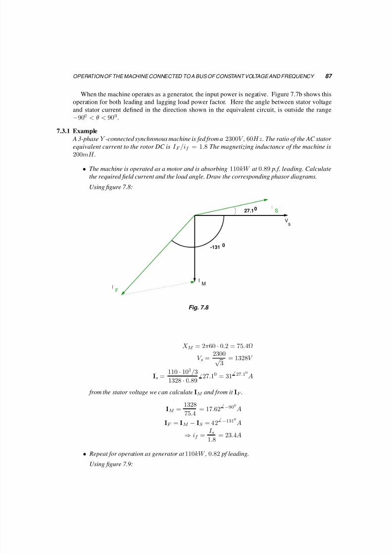
5/17/2018 Electrical Machines and Drives - slidepdf.com
http://slidepdf.com/reader/full/electrical-machines-and-drives-55ab59315f602 95/123
OPERATION OF THE MACHINE CONNECTED TO A BUS OF CONSTANT VOLTAGE AND FREQUENCY 87
When the machine operates as a generator, the input power is negative. Figure 7.7b shows thisoperation for both leading and lagging load power factor. Here the angle between stator voltage
and stator current defined in the direction shown in the equivalent circuit, is outside the range
−900 < θ < 900.
7.3.1 Example
A 3-phase Y -connected synchronous machine is fed from a 2300V , 60Hz. The ratio of the AC stator
equivalent current to the rotor DC is I F /if = 1.8 The magnetizing inductance of the machine is
200mH .
• The machine is operated as a motor and is absorbing 110kW at 0.89 p.f. leading. Calculate
the required field current and the load angle. Draw the corresponding phasor diagrams.
Using figure 7.8:
I
IM
I
sV
S
F
-1310
27.10
Fig. 7.8
X M = 2π60 · 0.2 = 75.4Ω
V s =2300√
3= 1328V
Is =110 · 103/3
1328·
0.8927.10 = 31
27.10A
from the stator voltage we can calculate IM and from it IF .
IM =1328
75.4= 17.62
−900A
IF = IM − IS = 42−1310A
⇒ if =I s
1.8= 23.4A
• Repeat for operation as generator at 110kW , 0.82 pf leading.
Using figure 7.9:

5/17/2018 Electrical Machines and Drives - slidepdf.com
http://slidepdf.com/reader/full/electrical-machines-and-drives-55ab59315f602 96/123
88 SYNCHRONOUS MACHINES AND DRIVES
MI
sV
I
35
3.56
IF
G
0
0
SI
-1450
Fig. 7.9
Ig = 33.735A ⇒ IS = 33.7−1450A
IF = IM − IS = 27.66 3.560A
⇒ if = 15.37A
• What is the maximum power the machine above can produce (or absorb) when operating as a
generator and at the field current just calculated?
We know that absorbed and produced power is:
P = −3V sI F cos β
for if = 15.37A we have I F = 27.66A , and P becomes maximum for β = 0 , hence:
P = 3 · 1328 · 27.66 = 110.2kW
• If the terminal voltage remains at 2300V , 60Hz , what is the minimal field current required to
maintain operation as a motor with load 70kW ?
Again here:
P = 2 · V sI f cos β = 3 · 1328 · I F = 70 · 103W
⇒ I F = 17.57A
7.4 OPERATION FROM A SOURCE OF VARIABLE FREQUENCY AND VOLTAGE
This operation requires that our synchronous machine is supplied by an inverter. The operation now
is entirely different than before. We no longer have an infinite bus, but rather whatever stator voltage
or current and frequency we desire. Moreover, with a space-vector controlled inverter, the phase
of this voltage or current can be arbitrarily set at any instant i.e. we can define the stator current

5/17/2018 Electrical Machines and Drives - slidepdf.com
http://slidepdf.com/reader/full/electrical-machines-and-drives-55ab59315f602 97/123
OPERATION FROM A SOURCE OF VARIABLE FREQUENCY AND VOLTAGE 89
or voltage space vector, and obtain it at will. The considerations for the motor operation are alsodifferent:
• There is no concern for absorbing or supplying reactive power. Instead, there is a limit on the
total stator current, determined by thermal considerations.
• There is a limit to the maximum voltage the source can supply, which leads to modifications
of the machine mode of operation at high speeds.
Operation from source of variable frequency and voltage is most common for Permanent Magnet
Machines, where the value of |IF| is constant.
In simple terms, when the machine is starting as a motor the frequency applied should be zero, but
the voltage space vector should be of such angle with respect to the rotor that torque is developed. as
discussed in the previous section. As torque develops, the machine accelerates, and the applied stator
currents have to create a rotating space vector leading the rotor flux. Voltage and frequency have tobe increased, so that this torque is maintained. It is important therefore to monitor the position of the
rotor in order to determine the location of the stator current or voltage space vector.
Two possible control techniques are implemented: either voltage control, where the stator voltage
space vector is determined and applied, or current control, where he stator current space vector is
applied.
For a fixed stator voltage and power (and torque) level, the stator losses are minimal when the
stator voltage and current are in phase. Figure 7.10 shows this condition.
Vs
IM
θ
β
IF
IS
Fig. 7.10 Operation of a synchronous PM drive at constant voltage and Frequency
Notice that as the power changes with the voltage constant two things happen:
1. The voltage space vector varies in amplitude and the magnetizing current changes with it.
2. The amplitude of IF stays constant, but its angle with respect to the voltage changes.
From the developed torque and speed we can calculate the frequency, the values of I M and I S ,
and the angle between the stator voltage space vector and the rotor, since
T =3 p
2ωsV sI s =
3 p
2LM I M I s (7.9)
I 2F = I 2M + I 2s (7.10)
and I F is a constant in PM machines.

5/17/2018 Electrical Machines and Drives - slidepdf.com
http://slidepdf.com/reader/full/electrical-machines-and-drives-55ab59315f602 98/123
90 SYNCHRONOUS MACHINES AND DRIVES
More common though is the case when the stator voltage is not constant. Here we monitor theposition of the rotor and since the rotor flux and rotor space current are attached to it, we are actually
monitoring the position of IF. To make matters simple we use this current rather than the stator
voltage as reference, as shown in figure 7.11.
I
V s
F
IMsI
jI F X M
jI s X M
γ
θ
Fig. 7.11 Operation of a synchronous PM drive below base speed
Although previous formulae for power and torque are still true they are not as useful. We create
new formulae that have the stator current I s and magnetizing current I M as variables. We also use
the angle γ , between IF and Is, since we can control it. Starting from what we already know:
P g = [VsI∗F] = [ jXM(IF + Is)I∗F] (7.11)
= [ jXMIFI∗F] + [ jXMIsI∗F] (7.12)
= X M [IsI∗F] = XMIsIF sin γ (7.13)
For a given torque minimum losses require minimum value of the stator current. To minimize the
value of I s with constant power and I F we choose γ = 90o and arrive at:
P g = X M [IsI∗F] = X M I sI F (7.14)
T = 3 p
2
P gωs
= 3 p
2LM [IsI∗F] = 3
p
2LM I sI F (7.15)
which means that for constant power the projection of the stator current on an axis perpendicular toIM is constant.
As the rotor speed increases, even if I M stays constant, the stator voltage V s = ωsLmI s increases.
At some speed ωsB , the required voltage exceeds the maximum the power source can provide. We
call this speed base speed; To increase the speed beyond it we no longer keep γ = 90o. On the other
hand at that speed we know that the voltage has reached its upper limit V s = V s,max, therefore the
value of I M = V s,max/X M is known. In this case, equations 7.9 and 7.10 become:
T =3 p
2ωsV sI s cos θ =
3 p
2LM I M I s cos θ (7.16)
I 2F = I 2M + I 2s + 2I M I s sin θ (7.17)

5/17/2018 Electrical Machines and Drives - slidepdf.com
http://slidepdf.com/reader/full/electrical-machines-and-drives-55ab59315f602 99/123
OPERATION FROM A SOURCE OF VARIABLE FREQUENCY AND VOLTAGE 91
s1I
IM2
jI F X M
jI
s1
X
M
jI s2 X M
θ1
θ2
V
I
1γ 2
γ
M1
I
s2
V s1
s2
F
I
Fig. 7.12 Field weakening of a PM AC motor. The two diagrams at are at the same frequency, but the secondone has γ > 90
o and lower V s
.
Figure 7.12 shows such an operation with the variables having the subscript 1. Note that we
calculate torque from power:
P = 3X M I SI F sin γ (7.18)
T =P
ωs
p
2= 3
p
2LM [ISI∗F] = 3
p
2LM I sI F sin γ (7.19)
7.4.1 Example A 3-phase, four pole, Y connected permanent magnet synchronous machine is rated 400V , 50Hz ,
50kV A. Its magnetizing inductance is 2.5mH and its equivalent field source current is 310A. We
can neglect stator resistance.
• The machine is operated as a generator at rated frequency. Determine the maximum and
minimum values of the stator phase voltage as the load current is varied from zero to rated
value at unity power factor.
The rated phase voltage is V s = 400/√
3 = 231V and the rated stator current is I s =50 · 103/3 · 231 = 72.2A. With no load and at rated frequency the phase voltage is:
V s = ωsLM I F = 2π50 · 2.5 · 10−3 · 310 = 243.5V
I the motor is operated at power factor, the stator current is collinear with the stator voltage,as in figure 7.13.
From the current triangle:
I 2M = I 2F − I 2s ⇒ I M =
3102 − 72.72 = 301.5A
and the stator voltage is:
V s = ωsLM I M = 236.8V
• The machine is now operated as a variable speed drive motor from a variable voltage, variable
frequency source. What should be the voltage and frequency in order to provide torque of
300Nm at 600rpm, if again we have unity power factor?

5/17/2018 Electrical Machines and Drives - slidepdf.com
http://slidepdf.com/reader/full/electrical-machines-and-drives-55ab59315f602 100/123
92 SYNCHRONOUS MACHINES AND DRIVES
SI
gI
Vs
IM
FI
Fig. 7.13
The machine has four poles, so
ωs =p
2600
2π
60= 20Hz
Torque can be expressed as a function of input power:
T = 3 p
2
1
ωsV sI s pf = 3
p
2ωs(ωsLM I M )I s =
3 p
2LM I M I s = 300N m
In addition to this equation we have from the current triangle for unity pf:I 2F = I 2M + I 2s = 3002
These two equations, solved together will give
I M = 303A I s = 66A or
I M = 66 I s = 303A
which leads to phase voltage and torque:
V s = ωsLM I M = 95.1V
P m =2
pωsT = 18.84kW
7.4.2 Example
A 2-pole, 3-phase Permanent Magnet synchronous generator is rated 230V (l-l) 10kV A , 400Hz.
Its magnetizing inductance is 0.6mH . First a test is performed: The rotor is externally driven at
rated speed with the stator open circuited and the line-line voltage is measured at 240V . Based on the result of this test determine the stator voltage and power angle when the stator
current, voltage and frequency are rated and the power factor of the load is 0.9 lagging.
From the test:
X M = ωsLM = 2π400 · 0.6 · 10−3 = 1.508Ω
V s = |IMXM| =240√
3⇒ I M = 91.9A

5/17/2018 Electrical Machines and Drives - slidepdf.com
http://slidepdf.com/reader/full/electrical-machines-and-drives-55ab59315f602 101/123
OPERATION FROM A SOURCE OF VARIABLE FREQUENCY AND VOLTAGE 93
but at no load I F = I M = 91.9A and it is constant
Now that we found I F , to the problem: At the operating point
I s =S √3V ll
=10 · 103√
3 · 230= 25.102A
pf = 0.9 ⇒ θ = −25.84o
from the geometry of the current triangle:
I 2M + I 2s − 2I M I S cosπ
2+ θ
= I 2F
⇒⇒ I 2M + 25.12 − 2 · 25.1 · I M · 0.436 = 91.92
⇒ I M = 100A
¡
£
¡
£
¤
£
¦
£
Fig. 7.14 Phasor diagram for this example
7.4.3 Example
A permanent magnet, Y connected, three-phase, 2-pole motor has I F = 40 and X M = 0.9Ω at
100Hz.
1. If it is absorbing P = 1.5kW at 100Hz with minimum stator current I s , calculate this current,the angle between Is and IF , the speed, the stator voltage (line-neutral) and the power factor.
The minimum current I s will exist when γ = (Is, IF) = 90o. Then:
P = 3X M I sI F ⇒ I s =1500
3 · 0.9 · 40= 13.89A
⇒ IM = IF + Is = 40 + 13.89 90o = 42.34
19.15oA
⇒ Vs = jωsLM IM = 38.12 109.15oV
the power factor is:
pf = cos(109.14o − 90o) = 0.946lagging
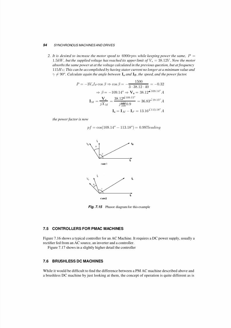
5/17/2018 Electrical Machines and Drives - slidepdf.com
http://slidepdf.com/reader/full/electrical-machines-and-drives-55ab59315f602 102/123
94 SYNCHRONOUS MACHINES AND DRIVES
2. It is desired to increase the motor speed to 6900rpm while keeping power the same, P =1.5kW , but the supplied voltage has reached its upper limit of V s = 38.12V . Now the motor
absorbs the same power at at the voltage calculated in the previous question, but at frequency
115Hz; This can be accomplished by having stator current no longer at a minimum value and
γ = 90o. Calculate again the angle between Is and IF , the speed, and the power factor.
P = −3V sI F cos β ⇒ cos β = − 1500
3 · 38.12 · 40= −0.32
⇒ β = −109.14o ⇒ Vs = 38.12 109.14oA
IM =Vs
jX M =
38.12 109.15o
j 115100
0.9= 36.83
19.15oA
Is = IM
−IF = 13.16
113.18oA
the power factor is now
pf = cos(109.14o − 113.18o) = 0.997leading
¡
£
¡
£
¤
£
¦
¡
£
¡
£
¤
£
¦
§
§
Fig. 7.15 Phasor diagram for this example
7.5 CONTROLLERS FOR PMAC MACHINES
Figure 7.16 shows a typical controller for an AC Machine. It requires a DC power supply, usually a
rectifier fed from an AC source, an inverter and a controller.
Figure 7.17 shows in a slightly higher detail the controller
7.6 BRUSHLESS DC MACHINES
While it would be difficult to find the difference between a PM AC machine described above and
a brushless DC machine by just looking at them, the concept of operation is quite different as is
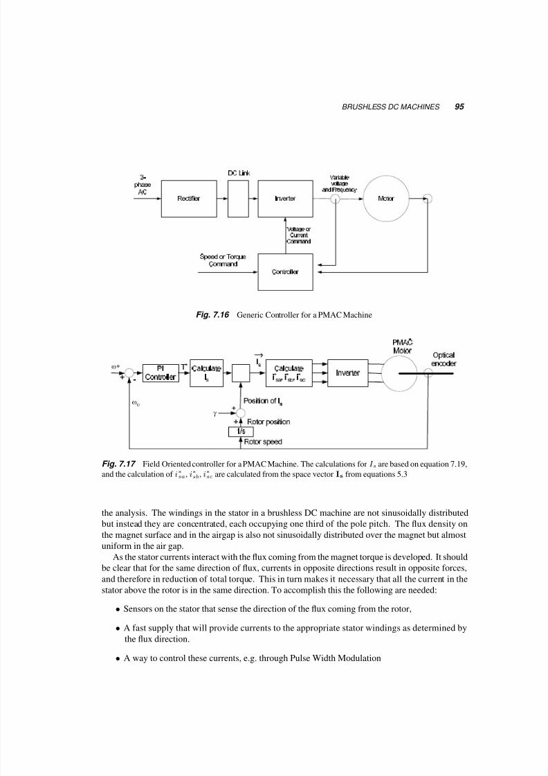
5/17/2018 Electrical Machines and Drives - slidepdf.com
http://slidepdf.com/reader/full/electrical-machines-and-drives-55ab59315f602 103/123
BRUSHLESS DC MACHINES 95
¡ ¢
£
¥ ¤
¡ ¦
§
©
¡ ¦
£
¡ ¦
£
¦
¨
£
¦
¡ ¦
¡
!
#
$ ¤
%
&
' ( '
0 1
2
3
4
1 5
' 6 2
' 7
8 9
( 2 @
A
2 7 B
C
D
¡ ¡
E
¦
F
¦ G
H
¡
I I ¨
E
&
4
1 5
' 6 2 4 (
P
A
( ( 2 7
5
P
4 Q Q ' 7
8
Fig. 7.16 Generic Controller for a PMAC Machine
¡
¢
£ ¤
¥
£ ¤
¦
§
¨
©
¨
§
¥
£
¦
§
¨
©
¨
§
¥
£
¦
¡
¥
¤
¨ ¨
£ ¤
!
"
#
$
%
¥
© §
¨
£ ¡ ©
&
£ ¤
'
(
)
0
¥
¤ ) % £ £
&
0
¥
¤ % )
¥
¡
)
¥
¡
1 2
3
4 5
¦
4
¥
¤
#
#
Fig. 7.17 Field Oriented controller for a PMAC Machine. The calculations for I s are based on equation 7.19,
and the calculation of i∗sa, i∗sb, i∗sc are calculated from the space vector Is from equations 5.3
the analysis. The windings in the stator in a brushless DC machine are not sinusoidally distributed
but instead they are concentrated, each occupying one third of the pole pitch. The flux density on
the magnet surface and in the airgap is also not sinusoidally distributed over the magnet but almost
uniform in the air gap.
As the stator currents interact with the flux coming from the magnet torque is developed. It should
be clear that for the same direction of flux, currents in opposite directions result in opposite forces,
and therefore in reduction of total torque. This in turn makes it necessary that all the current in the
stator above the rotor is in the same direction. To accomplish this the following are needed:
• Sensors on the stator that sense the direction of the flux coming from the rotor,
• A fast supply that will provide currents to the appropriate stator windings as determined by
the flux direction.
• A way to control these currents, e.g. through Pulse Width Modulation
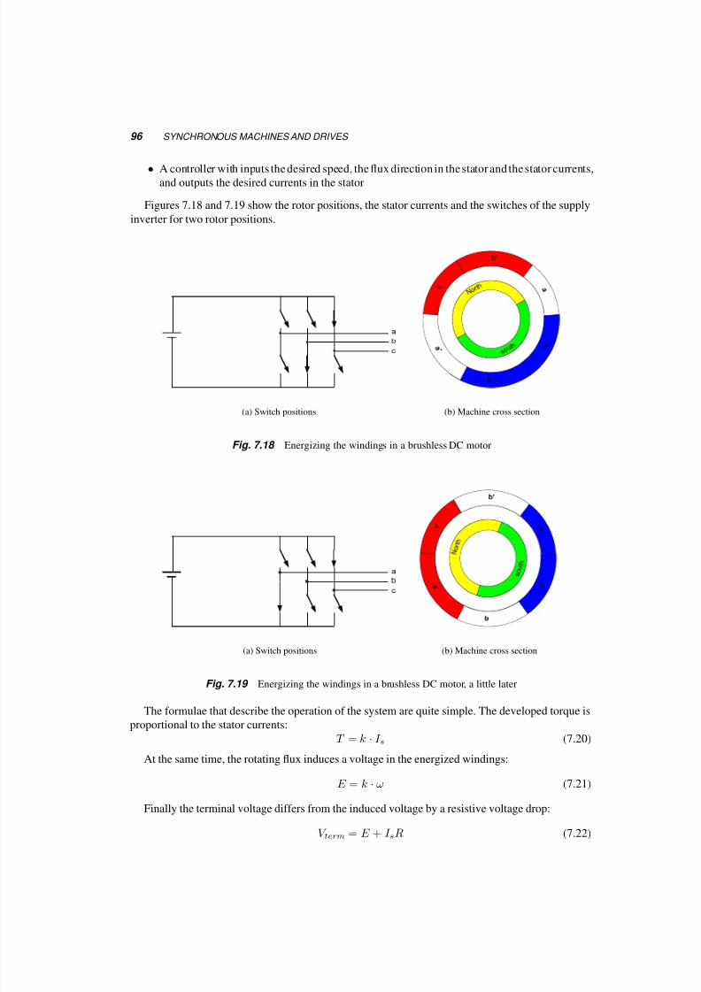
5/17/2018 Electrical Machines and Drives - slidepdf.com
http://slidepdf.com/reader/full/electrical-machines-and-drives-55ab59315f602 104/123
96 SYNCHRONOUS MACHINES AND DRIVES
• A controller with inputs the desired speed, the flux direction in the stator and the stator currents,and outputs the desired currents in the stator
Figures 7.18 and 7.19 show the rotor positions, the stator currents and the switches of the supply
inverter for two rotor positions.
¡
¢
(a) Switch positions (b) Machine cross section
Fig. 7.18 Energizing the windings in a brushless DC motor
¡
¢
(a) Switch positions (b) Machine cross section
Fig. 7.19 Energizing the windings in a brushless DC motor, a little later
The formulae that describe the operation of the system are quite simple. The developed torque is
proportional to the stator currents:
T = k · I s (7.20)
At the same time, the rotating flux induces a voltage in the energized windings:
E = k · ω (7.21)
Finally the terminal voltage differs from the induced voltage by a resistive voltage drop:
V term = E + I sR (7.22)

5/17/2018 Electrical Machines and Drives - slidepdf.com
http://slidepdf.com/reader/full/electrical-machines-and-drives-55ab59315f602 105/123
BRUSHLESS DC MACHINES 97
These equations are similar to those of a DC motor 4.4 - 4.6. This is the reason that although thismachine is entirely different from a DC motor, it is called brushless DC motor

5/17/2018 Electrical Machines and Drives - slidepdf.com
http://slidepdf.com/reader/full/electrical-machines-and-drives-55ab59315f602 106/123

5/17/2018 Electrical Machines and Drives - slidepdf.com
http://slidepdf.com/reader/full/electrical-machines-and-drives-55ab59315f602 107/123
8 Line Controlled Rectifiers
The idea here is to draw power from a 1-phase or 3-phase system to provide with DC a load. The
characteristics of the systems here are among others, that the devices used will turn themselves off
(commutate) and that the systems draw reactive power from the loads.
8.1 1- AND 3-PHASE CIRCUITS WITH DIODES
If the source is 1-phase, a diode is used and the load purely resistive, as shown in figure 8.1 things
are simple. When the source voltage is positive, the current flows through the diode and the voltage
of the source equals the voltage of the load. If the load includes an inductance and a source (e.g. a
battery we want to charge), as in figure 8.2, the diode will continue to conduct even when the load
voltage becomes negative as long as the current is maintained.
Fig. 8.1 Simple circuit with Diode and resistive Load
99

5/17/2018 Electrical Machines and Drives - slidepdf.com
http://slidepdf.com/reader/full/electrical-machines-and-drives-55ab59315f602 108/123
100 LINE CONTROLLED RECTIFIERS
Fig. 8.2 Smple Circuit with Diode and inductive load with voltage source
8.2 ONE -PHASE FULL WAVE RECTIFIER
More common is a single phase diode bridge rectifier 8.3. The load can be modelled with one of
two extremes: either as a constant current source, representing the case of a large inductance that
keeps the current through it almost constant, or as a resistor, representing the case of minimum line
inductance. We’ll study the first case with AC and DC side current and voltage waveforms shown in
figure 8.4.
If we analyze these waveforms, the output voltage will have a DC component V do:
V do =2
π
√2V s 0.9V s (8.1)
where V s is the RMS value of the input AC voltage. On the other hand the RMS value of the output
voltage will be
V s = V d (8.2)
containing components of higher frequency.
Similarly, on the AC side the current is not sinusoidal, but rather it changes abruptly between I dand −I d.
I s1 =2
π
√2I d = 0.9I d (8.3)

5/17/2018 Electrical Machines and Drives - slidepdf.com
http://slidepdf.com/reader/full/electrical-machines-and-drives-55ab59315f602 109/123
ONE -PHASE FULL WAVE RECTIFIER 101
Fig. 8.3 One-phase full wave rectifier
Fig. 8.4 Waveforms for a one-phase full wave rectifier with inductive load
and again the RMS values are the same
I d = I s (8.4)
Giving a total harmonic distortion
T HD =
I 2s − I 2s1
I s1∼= 48.43% (8.5)
It is important to notice that if the source has some inductance (and it usually does) commutation
will be delayed after the voltage has reached zero, until the current has dropped to zero as shown
in figure 8.5. This will lead to a decrease of the output DC voltage below what is expected from
formula 8.1.

5/17/2018 Electrical Machines and Drives - slidepdf.com
http://slidepdf.com/reader/full/electrical-machines-and-drives-55ab59315f602 110/123
102 LINE CONTROLLED RECTIFIERS
Fig. 8.5 One-phase full wave rectifier with inductive load and source inductance
8.3 THREE-PHASE DIODE RECTIFIERS
The circuit of figure 8.3 can be modified to handle three phases, without using 12 but rather 6 diodes,
as shown in figure 8.6. Figure 8.7 shows the AC side currents and DC side voltage for the case of
high load inductance. Similar analysis as before shows that on the DC side the voltage is:
V do =3
π
√2V LL = 1.35V LL (8.6)
From figure 8.6 it is obvious that on the AC side the rms current, I s is
I s =
2
3I d = 0.816I d (8.7)
while the fundamental current, i.e. the current at power frequency is:
I s1 =1
π
√6I d = 0.78I d (8.8)
Again, inductance on the AC side will delay commutation, causing a voltage loss, i.e. the DC
voltage will be less than that predicted by equation 8.6.

5/17/2018 Electrical Machines and Drives - slidepdf.com
http://slidepdf.com/reader/full/electrical-machines-and-drives-55ab59315f602 111/123
CONTROLLED RECTIFIERS WITH THYRISTORS 103
Fig. 8.6 Three-phase full-wave rectifier with diodes
Fig. 8.7 Waveforms of a three-phase full-wave rectifier with diodes and inductive load
8.4 CONTROLLED RECTIFIERS WITH THYRISTORS
Thyristors give us the ability to vary the DC voltage. Remember that to make a thyristor start
conducting, the thyristor has to be forward biased and a gate pulse provided to its gate. Also, to turn

5/17/2018 Electrical Machines and Drives - slidepdf.com
http://slidepdf.com/reader/full/electrical-machines-and-drives-55ab59315f602 112/123
104 LINE CONTROLLED RECTIFIERS
off a thyristor the current through it has to reverse direction for a short period of time, trr , and returnto zero.
8.5 ONE PHASE CONTROLLED RECTIFIERS
Figure 8.8 shows the same 1-phase bridge we have already studied, now with thyristors instead of
diodes, and figure 8.9 shows the output voltage and input current waveforms. In this figure α is the
delay angle, corresponding to the time we delay triggering the thyristors after they became forward
biased. Thyristors 1 and 2 are triggered together and of course so are 3 and 4. Each pair of thyristors
is turned off immediately (or shortly) after the other pair is turned on by gating. Analysis similar to
Fig. 8.8 One-phase full wave converter with Thyristors
that for diode circuits will give:
V do =2
π
√2V s cos α = 0.9V s cos α (8.9)
and the relation for the currents is the same
I s1 =2
π
√2I d = 0.9I d (8.10)
We should notice in figure 8.9 that the current waveform on the AC side is offset i time with respect
to the corresponding voltage by the same angle α, hence so is the fundamental of the current, leading
to a lagging power factor.On the DC side, only the DC component of the voltage carries power, since there is no harmonic
content in the current. On the AC side the power is carried only by the fundamental, since there are
no harmonics in the voltage.
P = V sI s1 cos α = V dI d (8.11)
8.5.1 Inverter Mode
If somehow the current on the DC side is sustained even if the voltage reverses polarity, then power
will be transferred from the DC to the AC side. The voltage on the D side can reverse polarity when

5/17/2018 Electrical Machines and Drives - slidepdf.com
http://slidepdf.com/reader/full/electrical-machines-and-drives-55ab59315f602 113/123
ONE PHASE CONTROLLED RECTIFIERS 105
Fig. 8.9 Waveforms of One-phase full wave converter with Thyristors
the delay angle exceeds 900, as long as the current is maintained. This can only happen when the
load voltage is as shown in figure 8.10, e.g. a battery.
Fig. 8.10 Operation of a one-phase controlled Converter as an inverter
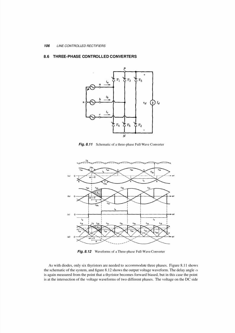
5/17/2018 Electrical Machines and Drives - slidepdf.com
http://slidepdf.com/reader/full/electrical-machines-and-drives-55ab59315f602 114/123
106 LINE CONTROLLED RECTIFIERS
8.6 THREE-PHASE CONTROLLED CONVERTERS
Fig. 8.11 Schematic of a three-phase Full-Wave Converter
Fig. 8.12 Waveforms of a Three-phase Full-Wave Converter
As with diodes, only six thyristors are needed to accommodate three phases. Figure 8.11 shows
the schematic of the system, and figure 8.12 shows the output voltage waveform. The delay angle αis again measured from the point that a thyristor becomes forward biased, but in this case the point
is at the intersection of the voltage waveforms of two different phases. The voltage on the DC side

5/17/2018 Electrical Machines and Drives - slidepdf.com
http://slidepdf.com/reader/full/electrical-machines-and-drives-55ab59315f602 115/123
*NOTES 107
is then:V do =
3
π
√2V LL cos α = 1.35V LL cos α (8.12)
while the power for both the AC and the DC side is
P = V dI do = 1.35V llId cos α =√
3V llI s1 cos α (8.13)
which leads to:
I s1 = 0.78I d (8.14)
Again if the delay angle α is extended beyond 900, the converter transfers power from the DC
side to the AC side, becoming an inverter. We should keep in mind, though, that even in this case
the converter is drawing reactive power from the AC side.
8.7 *NOTES
1. For both 1-phase and 3-phase controlled rectifier delay in α creates a phase displacement of
the phase current with respect to the phase voltage, equal to α. The cosine of this angle is the
power factor of the first harmonic.
2. For both motor and generator modes the controlled rectifier absorbs reactive power from the
three-phase AC system, although it can either absorb or produce real power. It also needs the
power line to commutate the thyristors. This means that inverter operation is possible only
when the rectifier is connected to a power line.
3. When a DC motor or a battery is connected to the terminals of a controlled rectifier and αbecomes greater then 900, the terminal DC voltage changes polarity, but the direction of the
current stays the same. This means that in order for the rectifier to draw power from battery
or a motor that operates as a generator turning in the same direction, the terminals haver to be
switched.

5/17/2018 Electrical Machines and Drives - slidepdf.com
http://slidepdf.com/reader/full/electrical-machines-and-drives-55ab59315f602 116/123
5/17/2018 Electrical Machines and Drives - slidepdf.com
http://slidepdf.com/reader/full/electrical-machines-and-drives-55ab59315f602 117/123
9 Inverters
Although the AC-to-DC converters we have already studied can transfer power from the DC side to
the AC system, they require the presence of such an AC system in order to commutate the thyristors
and provide the required reactive power. In this chapter we’ll study a similar system using devices
that we can turn both on and off, like GTOs, BJTs IGBTs and MOSFETs, which allows the transfer
of power from the DC source to any AC load. Figure 9.1 shows a typical application of a complete
system, where the supply power of constant voltage and frequency is rectified, filtered and theninverted to provide an output of desired voltage and frequency.
We’ll study first the operation of a single phase inverter and then we’ll expand to three-phases.
9.1 1-PHASE INVERTER
Figure 9.2 shows the operation of on leg of the inverter regardless of the number of phases. To
illustrate the point better, the input DC voltage is divided into two equal parts. When the upper
switch T A+ is closed, the output voltage V Ao will be 12
V d, and when the lower switch T A− is closed,
it will be − 12
V d. Deciding which switch to close in order to obtain a certain waveform will be
determined by the PWM comparison shown in figure 9.3. We define as the frequency modulation
index the ratio of the frequencies of the carrier (triangular wave) to the control signal:
mf =f sf 1
(9.1)
and as amplitude modulation index:
ma =V control
V tri(9.2)
Two comments here:
1. The output voltage in figure 9.3 at first look does not resemble the expected waveform (i.e. the
control signal). Its fundamental, though, does, and one can filter out the higher harmonics.
109

5/17/2018 Electrical Machines and Drives - slidepdf.com
http://slidepdf.com/reader/full/electrical-machines-and-drives-55ab59315f602 118/123
110 INVERTERS
Fig. 9.1 Typical variable voltage and frequency system supplied from a power system
Fig. 9.2 One leg of an inverter
Fig. 9.3 PWM scheme to determine which switch should be closed
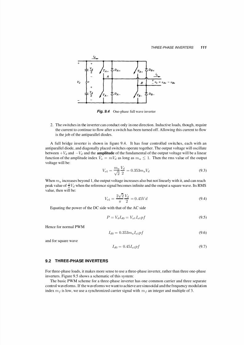
5/17/2018 Electrical Machines and Drives - slidepdf.com
http://slidepdf.com/reader/full/electrical-machines-and-drives-55ab59315f602 119/123
THREE-PHASE INVERTERS 111
Fig. 9.4 One-phase full wave inverter
2. The switches in the inverter can conduct only in one direction. Inductive loads, though, require
the current to continue to flow after a switch has been turned off. Allowing this current to flow
is the job of the antiparallel diodes.
A full bridge inverter is shown in figure 9.4. It has four controlled switches, each with an
antiparallel diode, and diagonally placed switches operate together. The output voltage will oscillate
between +V d and −V d and the amplitude of the fundamental of the output voltage will be a linear
function of the amplitude index V o = mV d as long as ma ≤ 1. Then the rms value of the output
voltage will be:
V o1 =ma√
2
V d2
= 0.353maV d (9.3)
When ma increases beyond 1, the output voltage increases also but not linearly with it, and can reachpeak value of 4π V d when the reference signal becomes infinite and the output a square wave. Its RMS
value, then will be:
V o1 =2√
2
π
V d2
= 0.45V d (9.4)
Equating the power of the DC side with that of the AC side
P = V dI d0 = V o1I o1 pf (9.5)
Hence for normal PWM
I d0 = 0.353maI o1 pf (9.6)
and for square wave
I d0 = 0.45I o1 pf (9.7)
9.2 THREE-PHASE INVERTERS
For three-phase loads, it makes more sense to use a three-phase inverter, rather than three one-phase
inverters. Figure 9.5 shows a schematic of this system:
The basic PWM scheme for a three-phase inverter has one common carrier and three separate
control waveforms. If the waveforms we want to achieve are sinusoidal and the frequency modulation
index mf is low, we use a synchronized carrier signal with mf an integer and multiple of 3.

5/17/2018 Electrical Machines and Drives - slidepdf.com
http://slidepdf.com/reader/full/electrical-machines-and-drives-55ab59315f602 120/123
112 INVERTERS
Fig. 9.5 Three-phase, full-wave inverter
Fig. 9.6 Three-phase Pulse Width Modulation

5/17/2018 Electrical Machines and Drives - slidepdf.com
http://slidepdf.com/reader/full/electrical-machines-and-drives-55ab59315f602 121/123
THREE-PHASE INVERTERS 113
Fig. 9.7 6-step operation of a PWM inverter
As long as ma is less than 1, the rms value of the fundamental of the output voltage is a linearfunction of it:
V LL1 =
√3
2√
2maV d 0.612maV d (9.8)
On the other hand, when the control voltage becomes infinite, the rms value of the fundamental
of the output voltage becomes:
V LL1 =
√3√2
4
π
V d2
0.78V d (9.9)
In this case the output voltage becomes rectangular and the operation is called 6-step operation, as
shown in figure 9.7b.
Equating the power on the DC and AC sides we obtain: Equating the power of the DC side with
that of the AC sideP = V dI d0 =
√3V ll1I o1 pf (9.10)
Hence for normal PWM
I d0 = 1.06maI o1 pf (9.11)
and for square wave
I d0 = 1.35I o1 pf (9.12)
Finally, there other ways to control the operation of an inverter. If it is not the output voltage
waveform we want to control, but rather the current, we can either impose a fast controller on the
voltage waveform, driven by the error in between the current signal and reference, or we can apply
a hysteresis band controller, shown for one leg of the inverter in figure 9.8
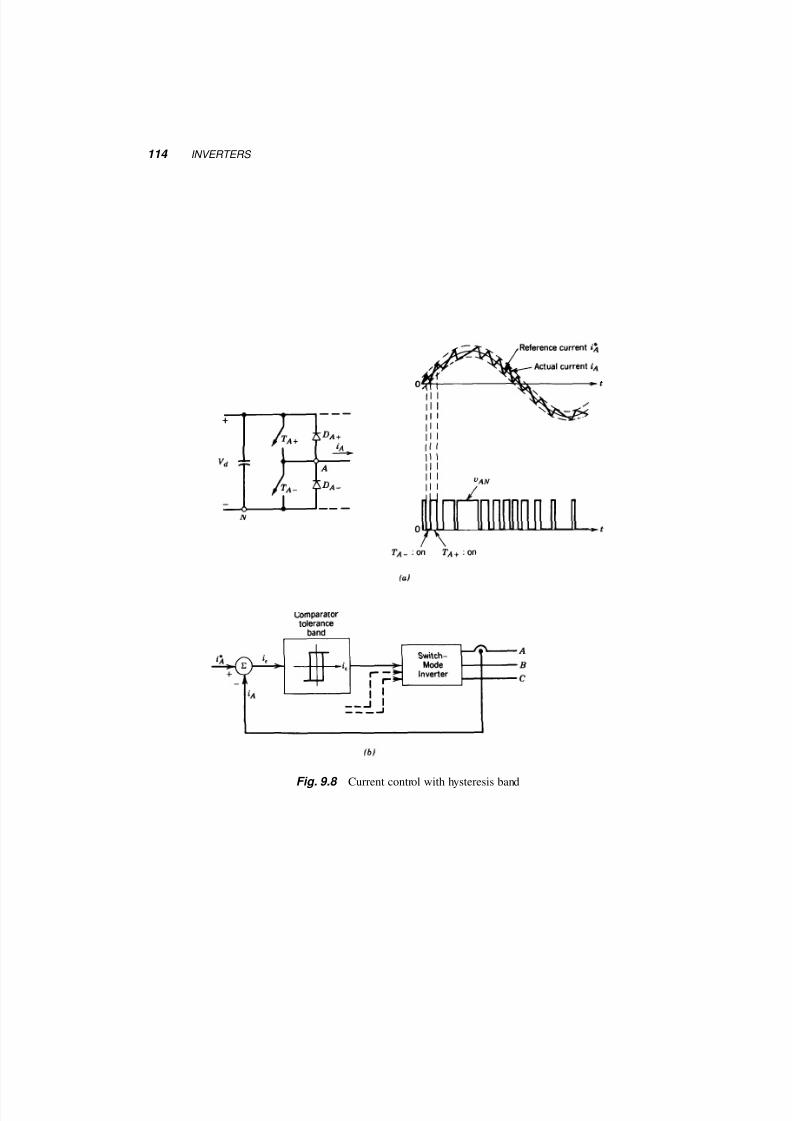
5/17/2018 Electrical Machines and Drives - slidepdf.com
http://slidepdf.com/reader/full/electrical-machines-and-drives-55ab59315f602 122/123
114 INVERTERS
Fig. 9.8 Current control with hysteresis band
5/17/2018 Electrical Machines and Drives - slidepdf.com
http://slidepdf.com/reader/full/electrical-machines-and-drives-55ab59315f602 123/123
THREE-PHASE INVERTERS 115
Notes
• With a sine-triangle PWM the harmonics of the output voltage s are of frequency around nf s,
where n is an integer and f s is the frequency of the carrier (triangle) waveform. The higher
this frequency is the easier to filter out these harmonics. On the other hand, increasing the
switching frequency increases proportionally the switching losses. For 6-step operation of a
3-phase inverter the harmonics are even except the triplen ones, i.e. they are of order 5, 7, 11,
13, 17 etc.
• When the load of an inverter is inductive the current in each phase remains positive after the
voltage in that phase became negative, i.e. after the top switch has been turned off. The
current then flows through the antiparallel diode of the bottom switch, returning power to the
DC link. The same happens of course when the bottom switch is turned off and the current
flows through the antiparallel diode of the top switch.