EGR 2201 Unit 10Second-Order Circuits

Read Alexander & Sadiku, Chapter 8. Homework #10 and Lab #10 due next

week. Quiz next week.

The circuits we studied last week are called first-order circuits because they are described mathematically by first-order differential equations.

We studied four kinds of first-order circuits: Source-free RC circuits

Source-free RL circuits

RC circuits with sources

RL circuits with sources

Review: Four Kinds of First-Order Circuits

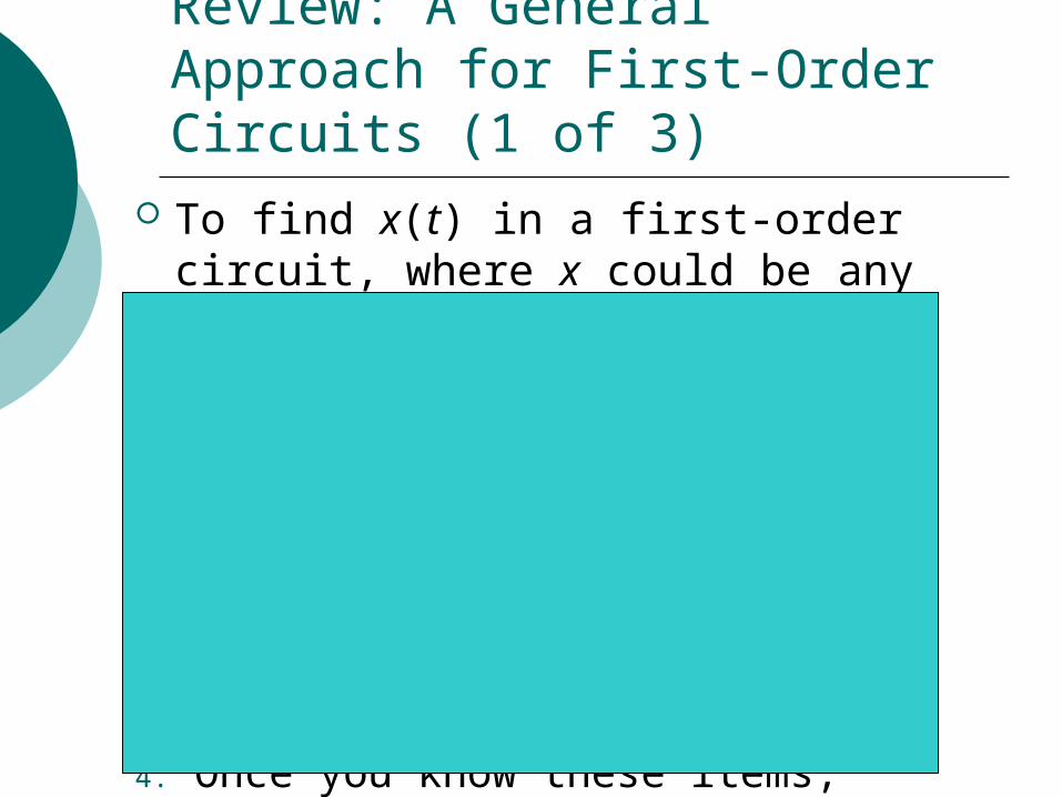
Review: A General Approach for First-Order Circuits (1 of 3)

To find x(t) in a first-order circuit, where x could be any current or voltage:

1. Find the quantity’s initial value .2. Find the quantity’s final value .

3. Find the time constant: for an RC circuit. for an RL circuit.

4. Once you know these items, solution is :

Review: A General Approach for First-Order Circuits (2 of 3)

The graph of the previous equation, is either:

A decaying exponential curve if the initial value x(0) is greater than the final value x().

Or a saturating exponential curve if the initial value x(0) is less than the final value x().

Review: A General Approach for First-Order Circuits (3 of 3)

Recall also that we can think of the complete response as being the sum of a transient response that dies away with time and a steady-state response that is constant and remains after the transient has died away:

Transient response

Steady-stateresponse

The textbook’s Sections 7.8 and 8.9 discuss using PSpice simulation software to perform transient analysis of first-order and second-order circuits.

We can also dothis with Multisim,as shown here.

Transient Analysis with Multisim

Our Goal: A General Approach for Second-Order Circuits

Next we will develop a general approach for analyzing more complicated circuits called second-order circuits.

Unfortunately the general approach for second-order circuits is quite a bit more complicated than the one for first-order circuits.

The circuits we’ll study are called second-order circuits because they are described mathematically by second-order differential equations.

Whereas first-order circuits contain a single energy-storing element (capacitor or inductor), second-order circuits contain two energy-storing elements. These two elements could both be

capacitors or both be inductors, but we’ll focus on circuits containing one capacitor and one inductor.

Second-Order Circuits

We’ll study four kinds of second-order circuits: Source-free series RLC circuits

Source-free parallel RLC circuits

Series RLC circuits with sources

Parallel RLC circuits with sources

Four Kinds of Second-Order Circuits

Recall that the term natural response refers to the behavior of source-free circuits.

And the term step response refers to the behavior of circuits in which a source is applied at some time.

So our goal in this unit is to understand the natural response of source-free RLC circuits, and to understand the step response of RLC circuits with sources.

Natural Response and Step Response

Our procedure will usually require us to find values of voltages or currents at the following three times: At t = 0, just before a switch is opened or

closed. At t = 0+, just after a switch is opened or

closed. As t , a long time after a switch is

opened or closed. Usually the circuit looks different at

these three times, so you’ll want to redraw the circuit for each of these times.

Redraw, Redraw, Redraw!

To completely solve a first-order differential equation, you need one initial condition, usually either: An initial inductor current i(0+), or An initial capacitor voltage v(0+).

To completely solve a second-order differential equation, you need two initial conditions, usually either: An initial inductor current i(0+) and its

derivative di(0+)/dt, or An initial capacitor voltage v(0+) and its

derivative dv(0+)/dt.

Finding Initial Values

To find initial derivative values such as dv(0+)/dt, we’ll rely on the basic relationships for capacitors and inductors:

For example, if we know a capacitor’s initial current i(0+), then we can use the left-hand equation above to find the initial derivative of that capacitor’s voltage, dv(0+)/dt.

Finding Initial Derivative Values

𝑣=𝐿𝑑𝑖𝑑𝑡

𝑖=𝐶𝑑𝑣𝑑𝑡

We’ll also rely on the fact that a capacitor’s voltage and an inductor’s current cannot change abruptly. Example: In this

circuit, i(0+) must be equal to i(0), and v(0+) must be equal to v(0).

Since these values must be equal, we don’t really need to distinguish between their values at time t = 0 and at time t = 0+. So we could just write i(0) instead of i(0+) and i(0).

Quantities that Cannot Change Abruptly

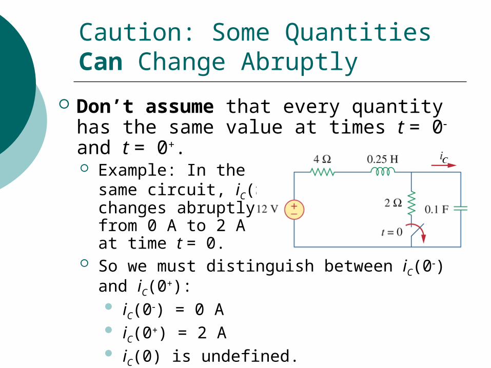
Don’t assume that every quantity has the same value at times t = 0 and t = 0+. Example: In the

same circuit, iC(t) changes abruptly from 0 A to 2 Aat time t = 0.

So we must distinguish between iC(0) and iC(0+): iC(0) = 0 A iC(0+) = 2 A iC(0) is undefined.

Caution: Some Quantities Can Change Abruptly

Our procedure will sometimes also require us to find final or “steady-state” values, such as: A final inductor current i() A final capacitor voltage v().

Usually these final values are easier to find than initial values, because: 1. We don’t have to worry about abrupt

changes as t , so we never need to distinguish between t and t +.

2. We don’t have to find derivatives of currents or voltages as t .

Finding Final Values

Consider the circuit shown. Assume that at time t=0, the inductor has initial current I0, and the capacitor has initial voltage V0.

As time passes, the initial energy in the capacitor and inductor will dissipate as currentflows through the resistor.

This results in changing current i(t), which we wish to calculate.

Natural Response of Source-Free Series RLC Circuit (1 of 2)

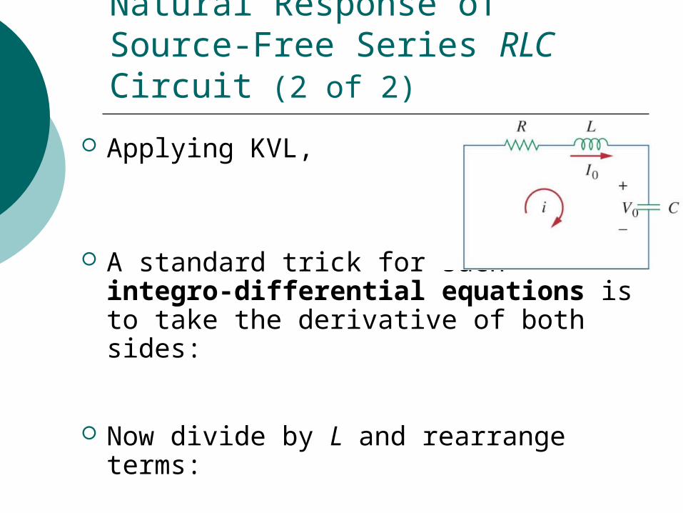
Applying KVL,

Natural Response of Source-Free Series RLC Circuit (2 of 2)

A standard trick for such integro-differential equations is to take the derivative of both sides:

Now divide by L and rearrange terms:

A Closer Look at Our Differential Equation

Our equation, , is a second-order linear differential equation with constant coefficients.

Such equations have been studied extensively, and we’ll outline the standard solution.

Solving Our Differential Equation (1 of 4)

To solve , first assume that the solution is of the form

where A and s are constants to be found. Plugging this into the equation yields:

Factoring out the common term,

Solving Our Differential Equation (2 of 4)

From it follows that:

This is called the characteristic equation of our original differential equation. Note that it is purely algebraic (no derivatives or integrals).

Now we can use the quadratic formula to solve for s. But first….

Solving Our Differential Equation (3 of 4)

For convenience we introduce two new symbols:

and We call the neper frequency, and we call

0 the undamped natural frequency. Then we can rewrite as:

Now use the quadratic formula….

Solving Our Differential Equation (4 of 4)

Applying the quadratic formula to gives two solutions for s, which we call the natural frequencies:

, Because of the square root, we must

distinguish three cases: > 0, called the overdamped case.

= 0, called the critically damped case.

< 0, called the underdamped case.

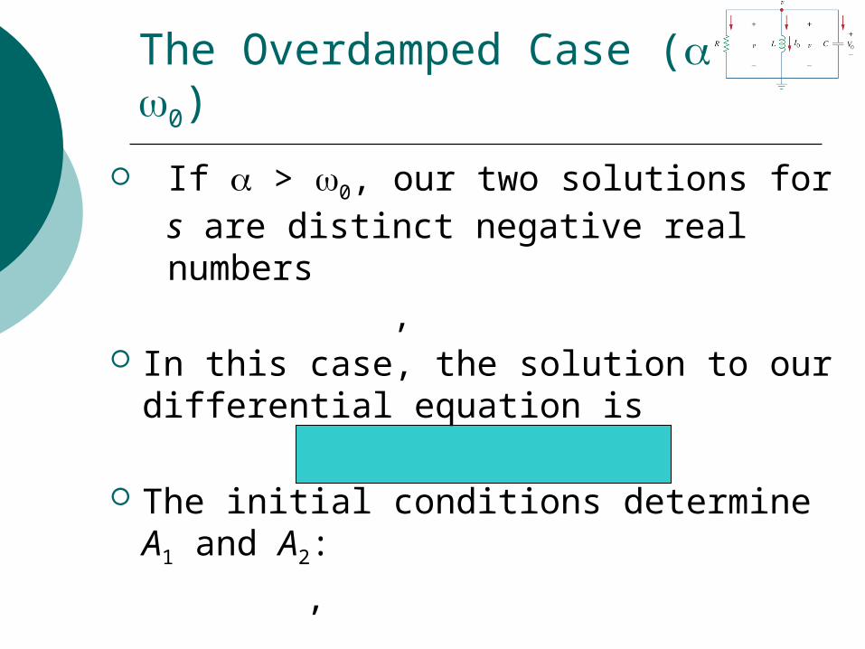
The Overdamped Case ( > 0)

If > 0, our two solutions for s are distinct negative real numbers:

, In this case, the solution to our differential

equation is

The initial conditions determine A1 and A2:

,

Real number

If = 0, our two solutions for s are equal to each other and to :

,

In this case, the solution to our differential equation is

The initial conditions determine A1 and A2:

,

The Critically Damped Case ( = 0)

Zero

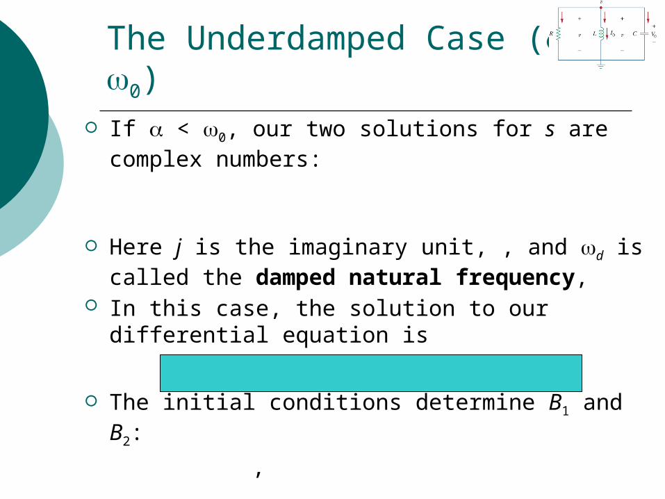
If < 0, our two solutions for s are complex numbers:

Here j is the imaginary unit, , and d is called the damped natural frequency,

In this case, the solution to our differential equation is

The initial conditions determine B1 and B2:

,

The Underdamped Case ( < 0)

Imaginary number

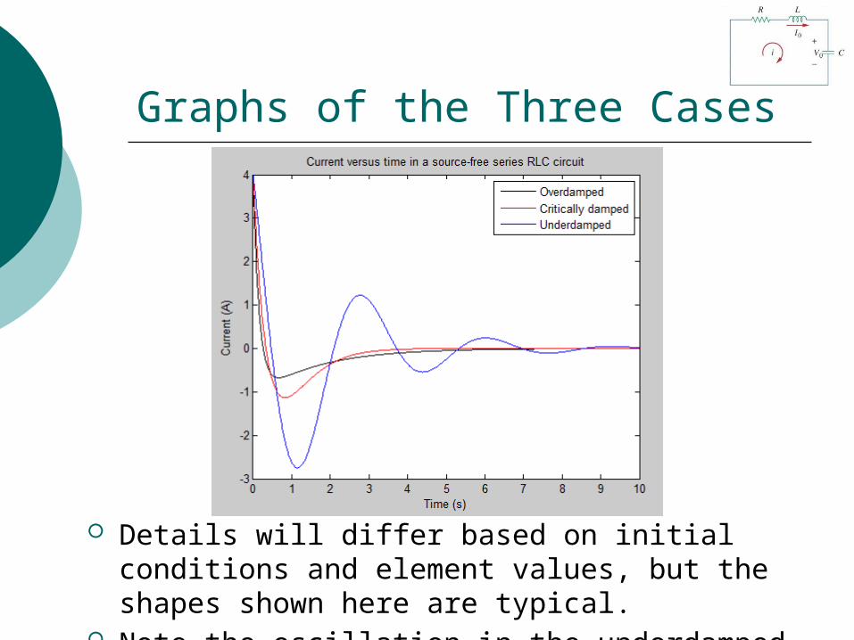
Graphs of the Three Cases

Details will differ based on initial conditions and element values, but the shapes shown here are typical.

Note the oscillation in the underdamped case.

The math for a source-free parallel circuit is almost the same as the math on the previous slides, except that:1. Now the variable in our differential

equation is v(t) instead of i(t).2. We define (the neper frequency)

to be equal to instead of .

Natural Response of Source-Free Parallel RLC Circuit (1 of 2)

By applying KCL and somealgebra, we get:

By assuming a solution of the form

we can derive the characteristic equation

Natural Response of Source-Free Parallel RLC Circuit (2 of 2)

Solving Our Differential Equation

For convenience we define:

and Note that 0 (the undamped natural

frequency) is the same as for series circuits, but (the neper frequency) is not.

Therefore, just as for series circuits,

We get the same three cases as before (overdamped, critically damped, and underdamped)….

The Overdamped Case ( > 0)

If > 0, our two solutions for s are distinct negative real numbers

, In this case, the solution to our differential

equation is

The initial conditions determine A1 and A2:

,

If = 0, our two solutions for s are equal to each other and to :

,

In this case, the solution to our differential equation is

The initial conditions determine A1 and A2:

,

The Critically Damped Case ( = 0)

If < 0, our two solutions for s are complex numbers:

Here j is the imaginary unit, , and d is called the damped natural frequency,

In this case, the solution to our differential equation is

The initial conditions determine B1 and B2:

,

The Underdamped Case ( < 0)

Graphs of the Three Cases

Details will differ based on initial conditions and element values, but the shapes shown here are typical.

Note the oscillation in the underdamped case.

A General Approach for Source-Free Series or Parallel RLC Circuits (1 of 3)

To find x(t) in a source-free series or parallel RLC circuit, where x could be any current or voltage:

1. Find the quantity’s initial value .

2. Find the quantity’s initial derivative .

3. Find the neper frequency: for a series RLC circuit. for a parallel RLC circuit.

4. Find the undamped natural frequency:

5. Compare to 0 to see whether circuit is overdamped, critically damped, or underdamped…

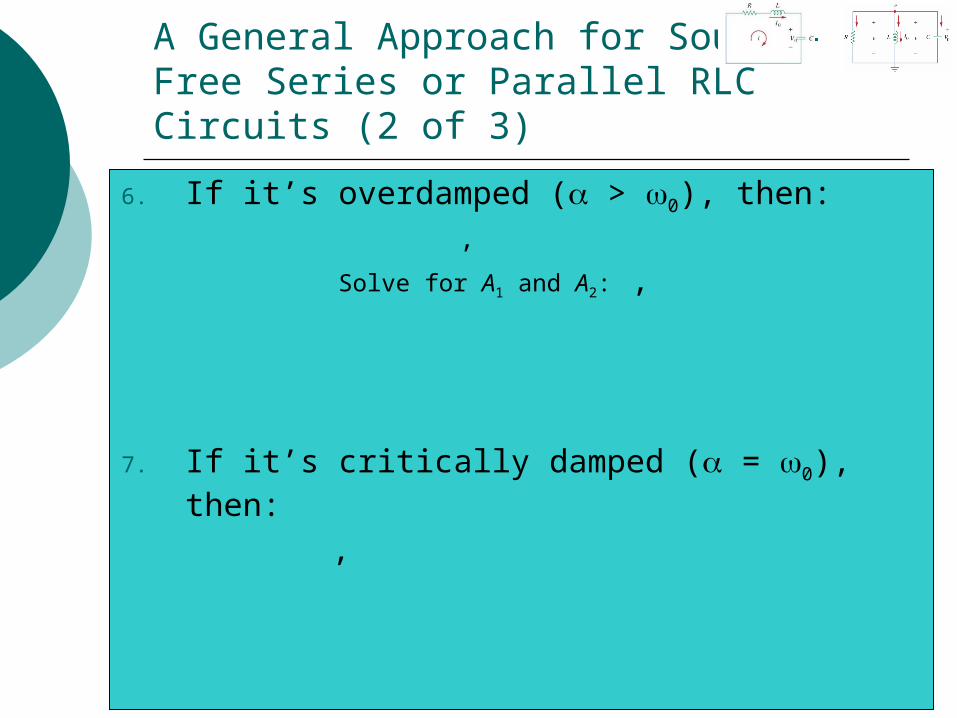
6. If it’s overdamped ( > 0), then: ,

Solve for A1 and A2: ,

7. If it’s critically damped ( = 0), then:

,

A General Approach for Source-Free Series or Parallel RLC Circuits (2 of 3)

8. If it’s underdamped ( < 0), then:

,

A General Approach for Source-Free Series or Parallel RLC Circuits (3 of 3)

Making Graphs in Word 2013 (1 of 4)

1. Select Insert > Chart on Word’s menu bar.

2. Select X Y (Scatter).

3. Select Scatter with Smooth Lines.

4. Click OK.

Making Graphs in Word 2013 (2 of 4)

5. Type your data values in this window.

6. You can create a new plot on the same chartby typing a new columnof data.

Making Graphs in Word 2013 (3 of 4)

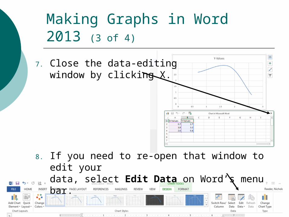
7. Close the data-editingwindow by clicking X.

8. If you need to re-open that window to edit yourdata, select Edit Data on Word’s menu bar.

Making Graphs in Word 2013 (4 of 4)

9. Add axis titles and a chart title by clicking the + andchecking the boxes.

10. Edit your axis titles and chart title by clicking them and

typing.

Typing Equations in Word 2013

1. Select Insert > Equation on Word’s menu bar.

2. Use the toolbar’s Structures section to create fractions, exponents, square roots, and more.

3. Use the toolbar’s Symbols section to insert basic math symbols, Greek letters, special operators, and more.