efficient strong integrators for linear stochastic systemssimonm/nsdes.pdf · efficient strong...

EFFICIENT STRONG INTEGRATORS FOR LINEAR STOCHASTIC

SYSTEMS

GABRIEL LORD∗, SIMON J.A. MALHAM∗† , AND ANKE WIESE∗

Abstract. We present numerical schemes for the strong solution of linear stochastic differen-tial equations driven by an arbitrary number of Wiener processes. These schemes are based on theNeumann (stochastic Taylor) and Magnus expansions. Firstly, we consider the case when the gov-erning linear diffusion vector fields commute with each other, but not with the linear drift vectorfield. We prove that numerical methods based on the Magnus expansion are more accurate in themean-square sense than corresponding stochastic Taylor integration schemes. Secondly, we derivethe maximal rate of convergence for arbitrary multi-dimensional stochastic integrals approximatedby their conditional expectations. Consequently, for general nonlinear stochastic differential equa-tions with non-commuting vector fields, we deduce explicit formulae for the relation between errorand computational costs for methods of arbitrary order. Thirdly, we consider the consequences intwo numerical studies, one of which is an application arising in stochastic linear-quadratic optimalcontrol.

Key words. linear stochastic differential equations, strong numerical methods, Magnus expan-sion, stochastic linear-quadratic control

AMS subject classifications. 60H10, 60H35, 93E20

1. Introduction. We are interested in designing efficient numerical schemes forthe strong approximation of linear Stratonovich stochastic differential equations ofthe form

yt = y0 +d∑

i=0

∫ t

0

ai(τ) yτ dW iτ , (1.1)

where y ∈ Rp, W 0 ≡ t, (W 1, . . . ,W d) is a d-dimensional Wiener process and a0(t)and ai(t) are given p × p coefficient matrices. We call ‘a0(t) y’ the linear drift vectorfield and ‘ai(t) y’ for i = 1, . . . , d the linear diffusion vector fields. We can express thestochastic differential equation (1.1) more succinctly in the form

y = y0 + K ◦ y , (1.2)

where K ≡ K0 + K1 + · · · + Kd and (Ki ◦ y)t ≡∫ t

0ai(τ) yτ dW i

τ . The solution ofthe integral equation for y is known as the Neumann series, Peano–Baker series,Feynman–Dyson path ordered exponential or Chen-Fleiss series

yt = (I − K)−1 ◦ y0 ≡ (I + K + K2 + K

3 + · · · ) ◦ y0 .

The flow-map or fundamental solution matrix St maps the initial data y0 to thesolution yt = St y0 at time t > 0. It satisfies an analogous matrix valued stochasticdifferential equation to (1.2) with the p × p identity matrix as initial data. Thelogarithm of the Neumann expansion for the flow-map is the Magnus expansion. Wecan thus write the solution to the stochastic differential equation (1.1) in the form

yt = (exp σt) y0 ,

∗Maxwell Institute for Mathematical Sciences and School of Mathematical and Computer Sciences,Heriot-Watt University, Edinburgh EH14 4AS, UK ([email protected], [email protected],[email protected]). (21/8/2007)

†SJAM would like to dedicate this paper to the memory of Nairo Aparicio, a friend and collabo-rator who passed away on 20th June 2005.

1

2 Lord, Malham and Wiese

where

σt = ln((I − K)−1 ◦ I

)≡ K ◦ I + K

2 ◦ I − 12 (K ◦ I)2 + · · · . (1.3)

See Magnus [41], Kunita [35], Azencott [3], Ben Arous [4], Strichartz [54], Castell [12],Burrage [7], Burrage and Burrage [8] and Baudoin [6] for the derivation and conver-gence of the original and also stochastic Magnus expansion; Iserles, Munthe–Kaas,Nørsett and Zanna [30] for a deterministic review; Lyons [38] and Sipilainen [53] forextensions to rough signals; Lyons and Victoir [40] for a recent application to prob-abilistic methods for solving partial differential equations; and Sussmann [56] for arelated product expansion.

In the case when the coefficient matrices ai(t) = ai, i = 0, . . . , d are constant andnon-commutative, the solution to the linear problem (1.1) is non-trivial and given bythe Neumann series or stochastic Taylor expansion (see Kloeden and Platen [33])

yneut =

∞∑

`=0

∑

α∈P`

Jα`···α1(t) aα1

· · · aα`y0 , (1.4)

where

Jα`···α1(t) ≡

∫ t

0

∫ ξ1

0

· · ·∫ ξ`−1

0

dWα`

ξ`· · · dWα2

ξ2dWα1

ξ1.

Here P` is the set of all combinations of multi-indices α = {α1, . . . , α`} of length `with αk ∈ {0, 1, . . . , d} for k = 1, . . . , `. There are some special non-commutative caseswhen we can write down an explicit analytical solution. For example the stochasticdifferential equation dyt = a1yt dW 1

t + yta2 dW 2t with the identity matrix as initial

data has the explicit analytical solution yt = exp(a1W1t ) · exp(a2W

2t ). However in

general we cannot express the Neumann solution series (1.4) in such a closed form.Classical numerical schemes such as the Euler-Maruyama and Milstein methods

correspond to truncating the stochastic Taylor expansion to generate global strongorder 1/2 and order 1 schemes, respectively. Stochastic Runge–Kutta numerical meth-ods have also been derived—see Kloeden and Platen [33] and Talay [57]. At the linearlevel, the Neumann, stochastic Taylor and Runge–Kutta type methods are equivalent.In the stochastic context, Magnus integrators have been considered by Castell andGaines [13], Burrage [7], Burrage and Burrage [8] and Misawa [46].

We present numerical schemes based on truncated Neumann and Magnus ex-pansions. Higher order multiple Stratonovich integrals are approximated across eachtime-step by their expectations conditioned on the increments of the Wiener processeson suitable subdivisions (see Newton [49] and Gaines and Lyons [22]). What is newin this paper is that we:

1. Prove the strong convergence of the truncated stochastic Magnus expansionfor small stepsize;

2. Derive uniformly accurate higher order stochastic integrators based on theMagnus expansion in the case of commuting linear diffusion vector fields;

3. Prove the maximal rate of convergence for arbitrary multi-dimensional stochas-tic integrals approximated by their conditional expectations;

4. Derive explicit formulae for the relation between error and computationalcosts for methods of arbitrary order in the case of general nonlinear, non-commuting governing vector fields.

Efficient stochastic integrators 3

Our results can be extended to nonlinear stochastic differential equations with anal-ogous conditions on the governing nonlinear vector fields, where the exponential Lieseries (replacing the Magnus expansion) can be evaluated using the Castell–Gainesapproach.

In the first half of this paper, sections 2–5, we focus on proving the convergence ofthe truncated Magnus expansion and establishing Magnus integrators that are moreaccurate than Neumann (stochastic Taylor) schemes of the same order. The numericalschemes we present belong to the important class of asymptotically efficient schemesintroduced by Newton [49]. Such schemes have the optimal minimum leading errorcoefficient among all schemes that depend on increments of the underlying Wienerprocess only. Castell and Gaines [13, 14] prove that the order 1/2 Magnus integratordriven by a d-dimensional Wiener process and a modified order 1 Magnus integratordriven by a 1-dimensional Wiener process are asymptotically efficient. We extendthis result of Castell and Gaines to an arbitrary number of driving Wiener processes.We prove that if we assume the linear diffusion vector fields commute, then an anal-ogously modified order 1 Magnus integrator and a new order 3/2 Magnus integratorare globally more accurate than their corresponding Neumann integrators.

There are several potential sources of cost contributing to the overall computa-tional effort of a stochastic numerical integration scheme. The main ones are theefforts associated with:

• Evaluation: computing (and combining) the individual terms and specialfunctions such as the matrix exponential;

• Quadrature: the accurate representation of multiple Stratonovich integrals.

There are usually fewer terms in the Magnus expansion compared to the Neumannexpansion to the same order, but there is the additional computational expense ofcomputing the matrix exponential. When the cost of computing the matrix exponen-tial is not significant, due to their superior accuracy we expect Magnus integratorsto be preferable to classical stochastic numerical integrators. This will be the casefor systems that are small (see Moler and Van Loan [47] and Iserles and Zanna [31])or for large systems when we only have to compute the exponential of a large sparsematrix times given vector data for which we can use Krylov subspace methods (seeMoler and Van Loan [47] and Sidje [52]). Magnus integrators are also preferable whenusing higher order integrators (applied to non-sparse systems of any size) when highaccuracies are required. This is because in this scenario, quadrature computationalcost dominates integrator effort.

In the second half of this paper, sections 6–8, we focus on the quadrature costassociated with approximating multiple Stratonovich integrals to a degree of accuracycommensurate with the order of the numerical method implemented. Our conclusionsapply generally to the case of nonlinear, non-commuting governing vector fields. Thegoverning set of vector fields and driving path process (W 1, . . . ,W d) generate theunique solution process y ∈ Rp to the stochastic differential equation (1.1). For ascalar driving Wiener process W the Ito map W 7→ y is continuous in the topology ofuniform convergence. For a d-dimensional driving processes with d ≥ 2 the UniversalLimit Theorem implies that the Ito map (W 1, . . . ,W d) 7→ y is continuous in the p-variation topology, in particular for 2 ≤ p < 3 (see Lyons [38], Lyons and Qian [39]and Malliavin [43]). Since Wiener paths with d ≥ 2 have finite p-variation for p > 2,approximations to y constructed using successively refined approximations to thedriving path will only converge to the correct solution y if we include informationabout the Levy chordal areas of the driving path (the L2-norm of the 2-variation of


a Wiener process is finite though). Hence if we want to implement a scheme usingadaptive stepsize we should consider order 1 or higher pathwise stochastic numericalmethods (see Gaines and Lyons [22]).

However simulating multiple Stratonovich integrals accurately is costly! For clas-sical accounts of this limitation on applying higher order pathwise stochastic numericalschemes see Kloeden and Platen [33, p. 367], Milstein [44, p. 92] and Schurz [51, p. 58]and for more recent results see Gaines and Lyons [21, 22], Wiktorsson [58], Cruzeiro,Malliavin and Thalmaier [17], Stump and Hill [55] and Giles [24, 25].

Taking a leaf from Gaines and Lyons [22] we consider whether it is computa-tionally cheaper to collect a set of sample data over a given time interval and thenevaluate the solution (conditioned on that sample data), than it is to evaluate thesolution frequently, say at every sample time. The resounding result here is that ofClark and Cameron [16] who prove that when the multiple Stratonovich integral J12 isapproximated by its expectation conditioned on intervening sample points, the max-imal rate of L2-convergence is of order h/Q1/2 where h is the integration steplengthand Q is the sampling rate. We extend this result to multiple Stratonovich integralsJα1,...,α`

of arbitrary order approximated by their expectation conditioned on inter-vening information sampled at the rate Q. Indeed we prove that the maximal rateof convergence is h`/2/Q1/2 when α1, . . . , α` are non-zero indices (and an improvedrate of convergence if some of them are zero). In practice the key information ishow the accuracy achieved scales with the effort required to produce it on the globalinterval of integration say [0, T ] where T = Nh. We derive an explicit formula forthe relation between the global error and the computational effort required to achieveit for a multiple Stratonovich integral of arbitrary order when the indices α1, . . . , α`

are distinct. This allows us to infer the effectiveness of strong methods of arbitraryorder for systems with non-commuting vector fields. For a given computational effortwhich method delivers the best accuracy? The answer not only relies on methodsthat are more accurate at a given order. It also is influenced by three regimes forthe stepsize that are distinguished as follows. In the first large stepsize regime theevaluation effort is greater than the quadrature effort; higher order methods producesuperior performance for given effort. Quadrature effort exceeds evaluation effort inthe second smaller stepsize regime. We show that in this regime when d = 2, or whend ≥ 3 and the order of the method M ≤ 3/2, then the global error scales with thecomputational effort with an exponent of −1/2. Here more accurate higher ordermethods still produce superior performance for given effort; but not at an increas-ing rate as the stepsize is decreased. However when d ≥ 3 for strong methods withM ≥ 2 the global error verses computational effort exponent is worse than −1/2 andthis distinguishes the third very small stepsize regime. The greater exponent meansthat eventually lower order methods will deliver greater accuracy for a given effort.

We have chosen to approximate higher order integrals over a given time step bytheir expectations conditioned on the increments of the Wiener processes on suit-able subdivisions. This is important for adaptive time-step schemes (Gaines andLyons [22]) and filtering problems where the driving processes (say W 1 and W 2) areobserved signals. However it should be noted that Wiktorsson [58] has provided apractical method for efficiently sampling the set of multiple Stratonovich multiple in-tegrals {Jij : i, j = 1, . . . , d} across a given time-step associated with a d-dimensionaldriving process (see Gilsing and Shardlow [23] for a practical implementation). Wik-torsson simulates the tail distribution in a truncated Karhunen–Loeve Fourier seriesapproximation of these integrals which produces a convergence rate of order hd3/2/Q


where Q is analogously the number of required independent normally distributedsamples.

Other potential sources of computational effort might be path generation andmemory access. Path generation effort depends on the application context. This costis at worst proportional to the quadrature effort where we could subsume it. Memoryaccess efforts depend on the processing and access memory environment. To revealhigher order methods (which typically require more path information) in the bestlight possible, we have ignored this effect.

Our paper is outlined as follows. We start in Section 2 by proving that theexponential of every truncation of the Magnus series converges to the solution of ourlinear stochastic differential equation (1.1). In Section 3 we define the strong errormeasures we use and how to compute them. Using these, we explicitly compare thelocal and then global errors for the Magnus and Neumann integrators in Section 4and thus establish our stated results for uniformly accurate Magnus integrators. InSection 5 we show that when the linear diffusion vector fields do not commute wecannot expect the corresponding order 1 Magnus integrator to in general be globallymore accurate than the order 1 Neumann integrator. We then turn our attention inSection 6 to the method of approximating multiple Stratonovich integrals by theirconditional expectations. We prove the maximal rate of convergence for an arbitrarymultiple Stratonovich integral in Section 6. We then use this result in Section 7 toshow how the global error scales with the computational effort for numerical schemesof arbitrary order. The shuffle algebra of multiple Stratonovich integrals generatedby integration by parts allows for different representions and therefore bases for thesolution of a stochastic differential equation. Some choices of basis representation aremore efficiently approximated than others and we investigate in Section 8 the impact ofthis choice. In Section 9 we present numerical experiments that reflect our theoreticalresults. To illustrate the superior accuracy of the uniformly accurate Magnus methodswe apply them to a stochastic Riccati differential system that can be reformulated as alinear system which has commuting diffusion vector fields. Since for the linear systemexpensive matrix-matrix multiplications can be achieved independent of the path, theNeumann method performs better than an explicit Runge–Kutta type method applieddirectly to the nonlinear Riccati system. We also numerically solve an explicit linearsystem with governing linear vector fields that do not commute for two and alsothree driving Wiener processes—Magnus integrators also exhibit superior accuracyin practice in these cases also. Lastly in Section 10, we outline how to extend ourresults to nonlinear stochastic differential equations and propose further extensionsand applications.

2. Strong convergence of truncated Magnus series. We consider here thecase when the stochastic differential equation (1.1) is driven by d Wiener processeswith constant coefficient matrices ai(t) = ai, i = 0, 1, . . . , d. The Neumann expansionhas the form shown in (1.4). We construct the Magnus expansion by taking thelogarithm of this Neumann series as in (1.3). In Appendix A we explicitly give theNeumann and Magnus expansions up to terms with L2-norm of order 3/2. Let σt

denote the truncated Magnus series

σt =∑

α∈Qm

Jα(t) cα , (2.1)

where Qm denotes the finite set of multi-indices α for which ‖Jα‖L2 is of order up toand including tm. Note that here m is a half-integer index, m = 1/2, 1, 3/2, . . .. The


terms cα are linear combinations of finitely many (more precisely exactly length α)products of the ai, i = 0, 1, . . . , d. Let |Qm| denote the cardinality of Qm.

Theorem 2.1 (Convergence). For any t ≤ 1, the exponential of the truncated

Magnus series, exp σt, is square-integrable. Further, if yt is the solution of the stochas-

tic differential equation (1.1), there exists a constant C(m) such that

∥∥yt − exp σt · y0

∥∥L2 ≤ C(m) tm+1/2 . (2.2)

Proof. First we show that exp σt ∈ L2. Using the expression (2.1) for σt, we seethat for any number k, (σt)

k is a sum of |Qm|k terms, each of which is a k-multipleproduct of terms Jαcα. It follows that

∥∥(σt)k∥∥

L2 ≤(

maxα∈Qm

‖cα‖op

)k

·∑

αi∈Qm

i=1,...,k

‖Jα(1)Jα(2) · · · Jα(k)‖L2 . (2.3)

Note that the maximum of the operator norm ‖ · ‖op of the coefficient matricesis taken over a finite set. Repeated application of the product rule reveals thatthe product Jα(i)Jα(j), where α(i) and α(j) are multi-indices of length `(α(i)) and

`(α(j)), is a linear combination of 2`(α(i))+`(α(j))−1 multiple Stratonovich integrals.Since `(α(i)) ≤ 2m for i = 1, . . . , k, each term ‘Jα(1)Jα(2) · · · Jα(k)’ in (2.3) is thus the

sum of at most 22mk−1 Stratonovich integrals Jβ . We also note that k ≤ `(β) ≤ 2mk.From equation (5.2.34) in Kloeden and Platen [33], every multiple Stratonovich

integral Jβ can be expressed as a finite sum of at most 2`(β)−1 multiple Ito integralsIγ with `(γ) ≤ `(β). Further, from Remark 5.2.8 in Kloeden and Platen [33], `(γ) +n(γ) ≥ `(β) + n(β), where n(β) and n(γ) denote the number of zeros in β and γ,respectively. From Lemma 5.7.3 in Kloeden and Platen [33],

‖Iγ‖L2 ≤ 2`(γ)−n(γ) t(`(γ)+n(γ))/2 .

Noting that `(γ) ≤ `(β) ≤ 2mk and `(γ) + n(γ) ≥ k, it follows that for t ≤ 1, wehave ‖Jβ‖L2 ≤ 24mk−1 tk/2. Since the right hand side of equation (2.3) consists of|Qm|k 22mk−1 Stratonovich integrals Jβ , we conclude that,

∥∥∥(σt

)k∥∥∥L2

≤(

maxα∈Qm

‖cα‖op · |Qm| · 26m · t1/2)k

.

Hence exp σt is square-integrable.Second we prove (2.2). Let yt denote Neumann series solution (1.4) truncated to

included terms of order up to and including tm. We have


∥∥L2 ≤

∥∥yt − yt

∥∥L2 +


∥∥L2 . (2.4)

We know yt ∈ L2 (see Gihman and Skorohod [23] or Arnold [2]). Furthermore, forany order m, yt corresponds to the truncated Taylor expansion involving terms oforder up to and including tm. Hence yt is a strong approximation to yt to that orderwith the remainder consisting of O(tm+1/2) terms (see Proposition 5.9.1 in Kloedenand Platen [33]). It follows from the definition of the Magnus series as the logarithmof the flow-map Neumann series, that the terms of order up to and including tm inexp σt · y0 correspond with yt; the error consists of O(tm+1/2) terms.


Convergence of approximations based on truncations of the stochastic Taylorexpansion has been studied in Kloeden and Platen [33], see Propositions 5.10.1, 5.10.2,and 10.6.3. Ben Arous [4] and Castell [12] prove the remainder of the exponential ofany truncation of the Magnus series is bounded in probability as t → 0 (in the fullnonlinear case). Burrage [7] shows that the first terms up to and including order 3/2Magnus expansion coincide with the terms in the Taylor expansion of the same order.Our result holds for any order in L2 for sufficiently small t. A more detailed analysisis needed to establish results concerning the convergence radius. Similar argumentscan be used to study the non-constant coefficient case with suitable conditions onthe coefficient matrices (see Proposition 5.10.1 in Kloeden and Platen [33] for thecorresponding result for the Taylor expansion).

Note that above and in subsequent sections, one may equally consider a stochasticdifferential equation starting at time t0 > 0 with square-integrable Ft0-measurableinitial data y0. Here (Ft)t≥0 denotes the underlying filtration.

3. Global and local error. Suppose Stn,tn+1and Stn,tn+1

are the exact andapproximate flow-maps across the interval [tn, tn+1], respectively; both satisfying theusual flow-map semi-group property: composition of flow-maps across successive inter-vals generates the flow-map across the union of those intervals. We call the differencebetween the exact and approximate flow-maps

Rtn,tn+1≡ Stn,tn+1

− Stn,tn+1(3.1)

the local flow remainder. For an approximation ytn+1across the interval [tn, tn+1] the

local remainder is thus Rtn,tn+1ytn

. Our goal here is to see how the leading orderterms in the local remainders accumulate, contributing to the global error.

Definition 3.1 (Strong global error). We define the strong global error associ-

ated with an approximate solution yT to the stochastic differential equation (1.1) over

the global interval of integration [0, T ] as E ≡ ‖yT − yT ‖L2 .

The global error can be decomposed additively into two components, the globaltruncation error due to truncation of higher order terms, and the global quadratureerror due to the approximation of multiple Stratonovich integrals retained in theapproximation. If [0, T ] = ∪N−1

n=0 [tn, tn+1] where tn = nh then for small stepsizeh = T/N we have

E =

∥∥∥∥∥

(0∏

n=N−1

Stn,tn+1−

0∏

n=N−1

Stn,tn+1

)y0

∥∥∥∥∥L2

=

∥∥∥∥∥

(N−1∑

n=0

Stn+1,tNRtn,tn+1

St0,tn

)y0

∥∥∥∥∥L2

+ O(max

n‖Rtn,tn+1

‖3/2L2 h−3/2

). (3.2)

The local flow remainder has the following form in the case of constant coefficientsai, i = 1, . . . , d, (see for example the integrators in Appendix A):

Rtn,tn+1=∑

α

Jα(tn, tn+1) cα .

Here α is a multi-index and the terms cα represent products or commutations of theconstant matrices ai. The Jα represent Stratonovich integrals (or linear combinations,of the same order, of products of integrals including permutations of α). The global


error E2 at leading order in the stepsize is thus

yT0

∑

α,β

(∑

n

E(Jα(tn, tn+1) Jβ(tn, tn+1)

)E

((Stn+1,tN

cαSt0,tn

)T(Stn+1,tN

cβSt0,tn

))

+∑

n6=m

E(Jα(tn, tn+1)

)E(Jβ(tm, tm+1)

)E

((Stn+1,tN

cαSt0,tn

)T(Stm+1,tN

cβSt0,tm

)))y0.

Hence in the global truncation error we distinguish between the diagonal sum con-sisting of the the first sum on the right-hand side above, and the off-diagonal sum

consisting of the second sum above with n 6= m.Suppose we include in our integrator all terms with local L2-norm up to and

including O(hM ). The leading terms Jαcα in Rtn,tn+1thus have L2-norm O(hM+1/2).

Those with zero expectation will contribute to the diagonal sum, generating O(hM )terms in the global error, consistent with a global order M integrator. However thosewith with non-zero expectation contribute to the off-diagonal double sum. They willgenerate O(hM−1/2) terms in the global error. We must thus either include them inthe integrator, or more cheaply, only include their expectations—the correspondingterms

(Jα − E(Jα)

)cα of order hM+1/2 in Rtn,tn+1

will then have zero expectationand only contribute through the diagonal sum—see for example Milstein [44, p. 12].This also guarantees the next order term in the global error estimate (3.2), whose

largest term has the upper bound maxn ‖Rtn,tn+1‖3/2

L2 h−3/2, only involves higher ordercontributions to the leading O(hM ) error.

Note that high order integrators may include multiple Stratonovich integral terms.We approximate these multiple integrals by their conditional expectations to the localorder of approximation hM+1/2 of the numerical method. Hence terms in the inte-

grator of the form Jαcα are in fact approximated by E(Jα|FQ)cα, their expectationconditioned on intervening path information FQ (see Section 6 for more details). Thisgenerates terms of the form

(Jα − E(Jα|FQ)

)cα in the local flow remainder, which

have zero expectation and hence contribute to the global error through the diagonalsum generating O(hM ) terms.

4. Uniformly accurate Magnus integrators. Our goal is to identify a classMagnus integrators that are more accurate than Neumann (stochastic Taylor) integra-tors of the same order for any governing set of linear vector fields (for the integratorsof order 1 and 3/2 we assume the diffusion vector fields commute). We thus com-pare the local accuracy of the Neumann and Magnus integrators through the leadingterms of their remainders. We consider the case of constant coefficient matrices ai,i = 0, 1, . . . , d.

The local flow remainder of a Neumann integrator Rneu is simply given by theterms not included in the flow-map Neumann approximation. Suppose σ is the trun-cated Magnus expansion and that ρ is the corresponding remainder, i.e. σ = σ + ρ.Then the local flow remainder Rmag associated with the Magnus approximation is

Rmag = exp σ − exp σ

= exp(σ + ρ

)− exp σ

= ρ + 12 (σρ + ρσ) + O(σ2ρ) . (4.1)

Hence the local flow remainder of a Magnus integrator Rmag is the truncated Magnusexpansion remainder ρ, and higher order terms 1

2 (σρ+ ρσ) that can contribute to the


global error at leading order through their expectations. For the integrators consideredin this section these higher order terms do not contribute in this way, however for theorder 1 integrator we consider in the next section they do.

Definition 4.1 (Uniformly accurate Magnus integrators). When the linear dif-

fusion vector fields commute so that [ai, aj ] = 0 for all i, j 6= 0, we define the order 1and order 3/2 uniformly accurate Magnus integrators by

σ(1)tn,tn+1

= J0a0 +

d∑

i=1

(Jiai + h2

12 [ai, [ai, a0]]),

and

σ(3/2)tn,tn+1

= J0a0 +d∑

i=1

(Jiai + 1

2 (Ji0 − J0i)[a0, ai] +h2

12 [ai, [ai, a0]]).

By uniformly we mean for any given set of governing linear vector fields (orequivalently coefficient matrices ai, i = 0, 1, . . . , d) for which the diffusion vectorfields commute, and for any initial data y0.

Theorem 4.2 (Global error comparison). For any initial condition y0 and suffi-

ciently small fixed stepsize h = tn+1 − tn, the order 1/2 Magnus integrator is globally

more accurate in L2 than the order 1/2 Neumann integrator. If in addition we assume

the linear diffusion vector fields commute so that [ai, aj ] = 0 for all i, j 6= 0, then the

order 1 and 3/2 uniformly accurate Magnus integrators are globally more accurate

in L2 than the corresponding Neumann integrators. In other words, if Emag denotes

the global error of the order 1/2 Magnus integrator or the uniformly accurate Magnus

integrators of order 1 or order 3/2, respectively, and Eneu is the global error of the

Neumann integrators of the corresponding order, then at each of those orders,

Emag ≤ Eneu . (4.2)

Proof. Let Rmag and Rneu denote the local flow remainders corresponding to theMagnus and Neumann approximations across the interval [tn, tn+1] with tn = nh. Adirect calculation reveals that

E((Rneu)TRneu

)= E

((Rmag)TRmag

)+ DM + O

(h2M+1/2

),

where if we set R ≡ Rneu − Rmag then

DM ≡ E(RTRmag

)+ E

((Rmag)TR

)+ E

(RTR

). (4.3)

We now show explicitly in each of the three cases of the theorem that at leading order:Rmag and R are uncorrelated and hence DM is positive semi-definite. This impliesthat the local remainder for the Neumann expansion is larger than that of the Magnusexpansion. Hereafter assume the indices i, j, k, l ∈ {1, . . . , d}.

For the order 1/2 integrators we have to leading order (see the form of the ex-pansions in Appendix A)

Rmag =∑

i<j

12 (Jij − Jji)[aj , ai] ,


and

R =∑

i

(Jii − 1

2h)a2

i +∑

i<j

12 (Jij + Jji)(ajai + aiaj) ,

which are uncorrelated by direct inspection.We henceforth assume [ai, aj ] = 0 for all i, j. For the uniformly accurate order 1

integrator we have to leading order (again see Appendix A)

Rmag =∑

i

12 (Ji0 − J0i)[a0, ai] ,

and

R = 12h2a2

0 +∑

i

12

(Ji0 + J0i)(a0ai + aia0) + 1

4h2(a2i a0 + a0a

2i )

+∑

i,j,k

(Jijk − E(Jijk)

)akajai ,

which again, by direct inspection are uncorrelated.For the uniformly accurate order 3/2 integrator the local flow remainders are

Rneu =∑

i

(Jii0 − 14h2)a0a

2i + Ji0iaia0ai + (J0ii − 1

4h2)a2i a0

+∑

i<j

((J0ji + J0ij)aiaja0 + Jj0iaia0aj

+ Ji0jaja0ai + (Jji0 + Jij0)a0aiaj

)

+∑

i,j,k,l

(Jijkl − E(Jijkl)

)alakajai ,

and

Rmag =∑

i

112 (J2

i J0 − h2 − 6Ji0i)[ai, [ai, a0]]

+∑

i<j

16

(J0JiJj − 3(Ji0j + Jj0i)

)[aj , [ai, a0]] .

Consequently we have

R = 112

∑

i

((6Ji0Ji − J2

i J0 − 2h2)a0a2i + 2(J2

i J0 − h2)aia0ai

+ (6J0iJi − J2i J0 − 2h2)a2

i a0

)

+ 16

∑

i<j

((3(JiJ0j + JjJ0i) − J0JiJj

)aiaja0

+(J0JiJj + 3(Ji0j − Jj0i)

)aja0ai

+(J0JiJj + 3(Jj0i − Ji0j)

)aia0aj

+(3(JiJj0 + JjJi0) − J0JiJj

)a0aiaj

)

+∑

i,j,k,l

(Jijkl − E(Jijkl)

)alakajai .


First we note that the terms in R of the form Jijklalakajai, for which at least threeof the indices distinct, are uncorrelated with any terms in Rmag. We thus focus onthe terms of this form with at most two distinct indices, namely

∑

i<j

(JiiJjj − 14h2)a2

ja2i +

∑

i6=j

JiiiJjaja3i +

∑

i

(Jiiii − 18h2)a4

i

and other remaining terms in R. Since E[Ji0i|Ji

]≡ h(J2

i − h)/6 and E[Ji0j |Ji, Jj

]≡

hJiJj/6 for i 6= j the following conditional expectations are immediate

E[(J2

i J0 − h2)(J2i J0 − h2 − 6Ji0i)|Ji

]= 0 ,

E[(Jiiii − 1

8h2)(J2i J0 − h2 − 6Ji0i)|Ji

]= 0 ,

E[(JiiJjj − 1

4h2)(J2i J0 − h2 − 6Ji0i)|Ji, Jj

]= 0 ,

E[(

J0JiJj + 3(Ji0j − Jj0i))(

J0JiJj − 3(Ji0j + Jj0i))|Ji, Jj

]= 0 ,

E[(JiiJjj − 1

4h2)(J0JiJj − 3(Ji0j + Jj0i)

)|Ji, Jj

]= 0 ,

E[JiiiJj

(J0JiJj − 3(Ji0j + Jj0i)

)|Ji, Jj

]= 0 .

Hence the expectations of the terms shown are also zero. Secondly, direct computationof the following expectations reveals

E((6J0iJi − J2

i J0 − 2h2)(J2i J0 − h2 − 6Ji0i)

)= 0 ,

E

((3(JiJ0j + JjJ0i) − J0JiJj

)(J0JiJj − 3(Ji0j + Jj0i)

))= 0 .

Hence Rmag and R are uncorrelated.The corresponding global comparison results (4.2) now follow directly in each of

the three cases above using that the local errors accumulate and contribute to theglobal error as diagonal terms in the standard manner described in detail at the endof Section 3. Note that we include the terms 1

12h2[ai, [ai, a0]] in the order 1 uniformlyaccurate Magnus integrator. These terms appear at leading order in the global re-mainder where they would otherwise generate a non-positive definite contribution toDM in (4.3).

Note that the Magnus integrator σ(1) is an order 1 integrator without the terms112h2[ai, [ai, a0]]. However they are cheap to compute and including them in theintegrator guarantees global superior accuracy independent of the set of governingcoefficient matrices.

5. Non-commuting linear diffusion vector fields. What happens when thelinear diffusion vector fields do not commute, i.e. we have [ai, aj ] 6= 0 for non-zeroindices i 6= j? Hereafter assume i, j, k ∈ {1, . . . , d}. Consider the case of order 1integrators. The local flow remainders are

Rneu =∑

i

(Ji0a0ai + J0iaia0) +∑

i,j,k

Jkjiaiajak

and

Rmag =∑

i

12 (Ji0 − J0i)[a0, ai] +

∑

i6=j

(Jiij − 1

2JiJij + 112J2

i Jj

)[ai, [ai, aj ]]

+∑

i<j<k

((Jijk + 1

2JjJki + 12JkJij − 2

3JiJjJk)[ai, [aj , ak]]

+ (Jjik + 12JiJkj + 1

2JkJji − 23JiJjJk)[aj , [ai, ak]]

).


Computing DM in (4.3) gives

DM = h2∑

i6=j

UTiijBUiij + h2

∑

i6=j 6=k

UTijkCUijk

where Uiij = (aja2i , aiajai, a

2i aj , a

3j , a0aj , aja0)

T ∈ R6p×p and in addition we have that

Uijk = (akajai, ajakai, akaiaj , aiakaj , ajaiak, aiajak)T ∈ R6p×p. Here B,C ∈ R6p×6p

consist of p × p diagonal blocks of the form bk`Ip and ck`Ip where

b = 1144

31 10 1 18 12 2410 4 10 0 0 01 10 31 18 24 1218 0 18 60 36 3612 0 24 36 36 3624 0 12 36 36 36

,

and

c = 136

4 1 1 1 1 −21 4 1 −2 1 11 1 4 1 −2 11 −2 1 4 1 11 1 −2 1 4 1−2 1 1 1 1 4

.

Again, c is positive semi-definite with eigenvalues { 16 , 1

6 , 16 , 1

6 , 0, 0}. However b has

eigenvalues { 16 , 1

48 (5 +√

41), 148 (5 −

√41), 0.94465, 0.0943205,−0.03897}, where the

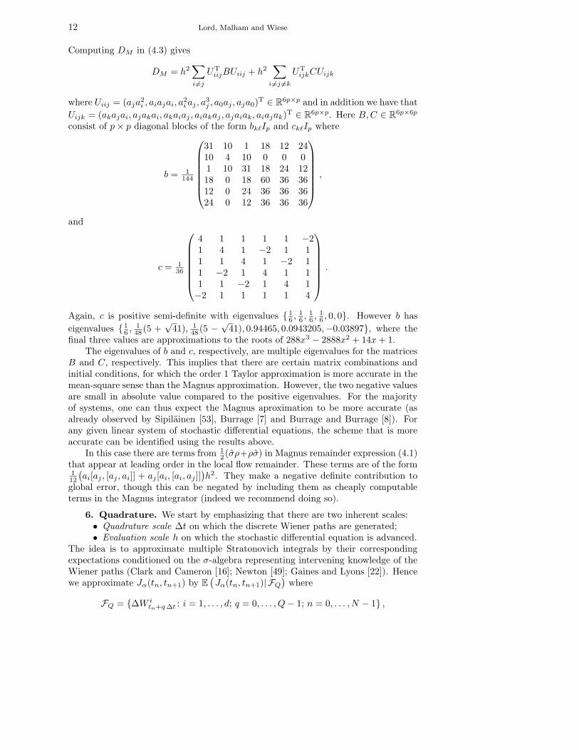
final three values are approximations to the roots of 288x3 − 2888x2 + 14x + 1.The eigenvalues of b and c, respectively, are multiple eigenvalues for the matrices

B and C, respectively. This implies that there are certain matrix combinations andinitial conditions, for which the order 1 Taylor approximation is more accurate in themean-square sense than the Magnus approximation. However, the two negative valuesare small in absolute value compared to the positive eigenvalues. For the majorityof systems, one can thus expect the Magnus aproximation to be more accurate (asalready observed by Sipilainen [53], Burrage [7] and Burrage and Burrage [8]). Forany given linear system of stochastic differential equations, the scheme that is moreaccurate can be identified using the results above.

In this case there are terms from 12 (σρ+ρσ) in Magnus remainder expression (4.1)

that appear at leading order in the local flow remainder. These terms are of the form112

(ai[aj , [aj , ai]] + aj [ai, [ai, aj ]]

)h2. They make a negative definite contribution to

global error, though this can be negated by including them as cheaply computableterms in the Magnus integrator (indeed we recommend doing so).

6. Quadrature. We start by emphasizing that there are two inherent scales:• Quadrature scale ∆t on which the discrete Wiener paths are generated;• Evaluation scale h on which the stochastic differential equation is advanced.

The idea is to approximate multiple Stratonovich integrals by their correspondingexpectations conditioned on the σ-algebra representing intervening knowledge of theWiener paths (Clark and Cameron [16]; Newton [49]; Gaines and Lyons [22]). Hencewe approximate Jα(tn, tn+1) by E

(Jα(tn, tn+1)| FQ

)where

FQ = {∆W itn+q ∆t : i = 1, . . . , d; q = 0, . . . , Q − 1; n = 0, . . . , N − 1} ,


with ∆W itn+q ∆t ≡ W i

tn+(q+1) ∆t − W itn+q ∆t, and Q∆t ≡ h, i.e. Q is the number of

Wiener increments. We extend the result of Clark and Cameron [16] on the maximumrate of convergence to arbitrary order multiple Stratonovich integrals.

Lemma 6.1 (Quadrature error). Suppose at least two of the indices in the multi-

index α = {α1, · · · , α`} are distinct. Define

j∗ ≡ min{j ≤ ` − 1: αi = αl , ∀ i, l > j} .

Let n(α) denote the number of zeros in α, and n∗(α) = n({αj∗ , . . . , α`}). Then the

L2 error in the multiple Stratonovich integral approximation E(Jα(tn, tn+1)| FQ

)is

∥∥Jα(tn, tn+1) − E(Jα(tn, tn+1)| FQ

)∥∥L2 = O

(h(`+n(α))/2

Q(n∗(α)+1)/2

). (6.1)

Proof. For any s, t, we write for brevity

Jα(s, t) = E(Jα(s, t) |FQ

).

We define α−k as the multi-index obtained by deleting the last k indices, that isα−k = {α1, · · · , α`−k}. We set τq ≡ tn + q∆t, where q = 0, . . . , Q − 1. Then

Jα(tn, tn+1) =

Q−1∑

q=0

∫ τq+1

τq

Jα−1(tn, τ) dWα`τ

=

Q−1∑

q=0

(`−1∑

k=1

Jα−k(tn, τq)Jα`−k+1,...,α`(τq, τq+1) + Jα(τq, τq+1)

).

Thus we have

Jα(tn, tn+1) − Jα(tn, tn+1)

=

Q−1∑

q=0

(`−1∑

k=1

(Jα−k(tn, τq) − Jα−k(tn, τq)

)Jα`−k+1,...,α`

(τq, τq+1)

+ Jα−k(tn, τq)(Jα`−k+1,...,α`

(τq, τq+1) − Jα`−k+1,...,α`(τq, τq+1)

)

+ Jα(τq, τq+1) − Jα(τq, τq+1)

). (6.2)

We prove the assertion by induction over `. For ` = 2, the first two terms in thesum (6.2) are zero and

∥∥∥∥Q−1∑

q=0

(Jα(τq, τq+1) − Jα(τq, τq+1)

)∥∥∥∥2

2

= O(Q(∆t)`+n(α)

)

= O(

h`+n(α)

Q`+n(α)−1

)

= O(

h`+n(α)

Qn∗(α)+1

).

Here we have used that fact that ` = 2, j∗ = 1 and thus n(α) = n∗(α).


Assume now that ` > 2. We will investigate the order of each of the three types ofterms in (6.2) separately. If at least two indices in α−k are distinct, then by inductionhypothesis

∥∥Jα−k(tn, τq) − Jα−k(tn, τq)∥∥2

2= O

((τq − tn)`−k+n(α−k)

qn∗(α−k)+1

),

and since τq − tn = q∆t and Q∆t = h, we have for each k = 1, . . . , ` − 1,

Q−1∑

q=0

∥∥(Jα−k(tn, τq) − Jα−k(tn, τq))Jα`−k+1,...,α`)(τq, τq+1)

∥∥2

2

= O(

h`+n(α)

Qn∗(α−k)+n(α)−n(α−k)+k

).

Note that we have

n∗(α−k) + n(α) − n(α−k) + k ≥ n∗(α) + k ≥ n∗(α) + 1 . (6.3)

If all indices in α−k are equal, then∥∥Jα−k(tn, τq) − Jα−k(tn, τq)

∥∥2

2= 0.

For the second term in (6.2) we have for each k = 1, . . . , ` − 1,

Q−1∑

q=0

∥∥Jα−k(tn, τq)(Jα`−k+1,...,α`

(τq, τq+1) − Jα`−k+1,...,α`(τq, τq+1)

)∥∥2

2

=

0 , if α` = . . . = α`−k+1 ,

O(

h`+n(α)

Qn(α)−n(α−k)+k−1

), otherwise .

Note that in the second of these cases

n(α) − n(α−k) + k − 1 ≥ n∗(α) + 1 . (6.4)

For the third term we have

Q−1∑

q=0

∥∥Jα(τq, τq+1) − Jα(τq, τq+1)∥∥2

2= O

(h`+n(α)

Q`+n(α)−1

).

Again, note that we have

` + n(α) − 1 ≥ n∗(α) + 1 . (6.5)

Equality holds in at least one of (6.3) to (6.5). To see this we distinguish thecase when the last two indices are equal, α`−1 = α`, and the case when the last twoindices are distinct, α`−1 6= α`. If α`−1 = α`, then

n∗(α−1) + n(α) − n(α−1) = n∗(α) .

Since in this case at least two indices in α−1 are distinct, equality holds for k = 1in (6.3). If α`−1 6= α`, then

n∗(α) = n(α) − n(α−2) ,


and thus equality holds for k = 2 in (6.4). Hence the lemma follows.Note that each multiple Stratonovich integral Jα(tn, tn+1) can be thought of as

an `-dimensional topologically conical volume in (W 1, . . . ,W `)-space. The surface ofthe conical volume is panelled with each panel distinguished by a double Stratonovichintegral term involving two consecutive indices from α. The edges between the panelsare distinguished by a triple integral and so forth. The conditional expectation ap-proximation E

(Jα(tn, tn+1)| FQ

)can also be decomposed in this way. In the L2-error

estimate for this approximation, the leading terms are given by sums over the panelswhich also confirm the estimate (6.1).

Approximations of multiple Stratonovich integrals constructed using their condi-tional expectations are intimately linked to those constructed using paths W i

t thatare approximated by piecewise linear interpolations of the intervening sample points.The difference between the two approaches are asymptotically smaller terms. Formore details see Wong and Zakai [59], Kloeden and Platen [33], Hofmann and Muller-Gronbach [29] and Gyongy and Michaletzky [27].

7. Global error vs computational effort. We examine in detail the step-size/accuracy regimes for which higher order stochastic integrators are feasible andalso when they become less efficient than lower order schemes. In any strong simula-tion there are two principle sources of computational effort. Firstly there is evaluationeffort Ueval associated with evaluating the vector fields, their compositions and anyfunctions such as the matrix exponential. Secondly there is the quadrature effort U quad

associated with approximating multiple stochastic integrals to an accuracy commen-surate with the order of the method. For a numerical approximation of order M thecomputational evaluation effort measured in flops over N = Th−1 evaluation steps is

Ueval = (cMp2 + cE)Th−1 .

Here p is the size of the system, cM represents the number of scalar-matrix multipli-cations and matrix-matrix additions for the order M truncated Magnus expansion,and cE is the effort required to compute the matrix exponential. Note that if we im-plement an order 1/2 method there is no quadrature effort. Hence since E = O(h1/2)we have E = O

((Ueval)−1/2

).

Suppose we are required to simulate Jα1···α`(tn, tn+1) with all the indices distinct

with a global error of order hM ; naturally ` ≥ 2 and M ≥ `/2.Lemma 7.1. The quadrature effort U measured in flops required to approximate

Jα1···α`(tn, tn+1) with a global error of order hM when all the indices are distinct and

non-zero, is to leading order in h:

U = O(h−β(M,`)

),

where

β(M, `) = (` − 1)(2M + 1 − `) + 1 .

Since we stipulate the global error associated with the multiple integral approximation

to be E = O(hM ), we have

E = O(U−M/β(M,`)

).

Proof. The quadrature effort required to construct E(Jα1···α`

(tn, tn+1)| FQ

),

which is a (`− 1)-multiple sum, over [0, T ] is U = O(Q`−1N) with N = Th−1. Using


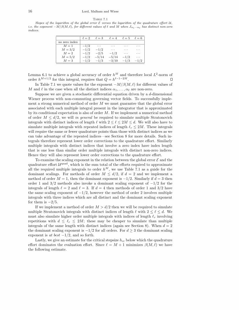
Table 7.1Slopes of the logarithm of the global error E verses the logarithm of the quadrature effort U ,

i.e. the exponent −M/β(M, `), for different values of ` and M when Jα1···α`has distinct non-zero

indices.

` = 2 ` = 3 ` = 4 ` = 5 ` = 6no zero index

M = 1 −1/2 · · · · · · · · · · · ·

M = 3/2 −1/2 −1/2 · · · · · · · · ·

M = 2 −1/2 −2/5 −1/2 · · · · · ·

M = 5/2 −1/2 −5/14 −5/14 −1/2 · · ·

M = 3 −1/2 −1/3 −3/10 −1/3 −1/2

Lemma 6.1 to achieve a global accuracy of order hM and therefore local L2-norm oforder hM+1/2 for this integral, requires that Q = h`−1−2M .

In Table 7.1 we quote values for the exponent −M/β(M, `) for different values ofM and ` in the case when all the distinct indices α1, . . . , α` are non-zero.

Suppose we are given a stochastic differential equation driven by a d-dimensionalWiener process with non-commuting governing vector fields. To successfully imple-ment a strong numerical method of order M we must guarantee that the global errorassociated with each multiple integral present in the integrator that is approximatedby its conditional expectation is also of order M . If we implement a numerical methodof order M ≤ d/2, we will in general be required to simulate multiple Stratonovichintegrals with distinct indices of length ` with 2 ≤ ` ≤ 2M ≤ d. We will also have tosimulate multiple integrals with repeated indices of length `r ≤ 2M . These integralswill require the same or fewer quadrature points than those with distinct indices as wecan take advantage of the repeated indices—see Section 8 for more details. Such in-tegrals therefore represent lower order corrections to the quadrature effort. Similarlymultiple integrals with distinct indices that involve a zero index have index lengththat is one less than similar order multiple integrals with distinct non-zero indices.Hence they will also represent lower order corrections to the quadrature effort.

To examine the scaling exponent in the relation between the global error E and thequadrature effort Uquad, which is the sum total of the efforts required to approximateall the required multiple integrals to order hM , we use Table 7.1 as a guide for thedominant scalings. For methods of order M ≤ d/2, if d = 2 and we implement amethod of order M = 1, then the dominant exponent is −1/2. Similarly if d = 3 thenorder 1 and 3/2 methods also invoke a dominant scaling exponent of −1/2 for theintegrals of length ` = 2 and ` = 3. If d = 4 then methods of order 1 and 3/2 havethe same scaling exponent of −1/2, however the method of order 2 involves multipleintegrals with three indices which are all distinct and the dominant scaling exponentfor them is −2/5.

If we implement a method of order M > d/2 then we will be required to simulatemultiple Stratonovich integrals with distinct indices of length ` with 2 ≤ ` ≤ d. Wemust also simulate higher order multiple integrals with indices of length `r involvingrepetitions with d ≤ `r ≤ 2M ; these may be cheaper to simulate than multipleintegrals of the same length with distinct indices (again see Section 8). When d = 2the dominant scaling exponent is −1/2 for all orders. For d ≥ 3 the dominant scalingexponent is at best −1/2, and so forth.

Lastly, we give an estimate for the critical stepsize hcr below which the quadratureeffort dominates the evaluation effort. Since ` = M + 1 minimizes β(M, `) we havethe following estimate.


Corollary 7.2. For the case of general non-commuting governing vector fields

and a numerical approximation of order M , we have U eval ≥ Uquad if and only if

h ≥ hcr where the critical stepsize

hcr = O((

T (cMp2 + cE))−1/(1−β(M,`max))

),

where `max = max{d,M + 1}.In practice when we implement numerical methods for stochastic differential equa-

tions driven by a d-dimensional Wiener process we expect that for h ≥ hcr the evalu-ation effort dominates the compuational cost. In this scenario integrators of order Mscale like their deterministic counterparts. Consider what we might expect to see in alog-log plot of global error verses computational cost. As a function of increasing com-putational cost we expect the global error for each method to fan out with slope −M ,with higher order methods providing superior accuracy for a given effort. Howeveronce the quadrature effort starts to dominate, the scaling exponents described abovetake over. When d = 2 for example and all methods dress themselves with the scalingexponent −1/2, then we expect to see parallel graphs with higher order methods stillproviding superior accuracy for a given cost. However higher order methods thatassume a scaling exponent worse than −1/2 will eventually re-intersect the graphs oftheir lower order counterparts and past that regime should not be used.

Note that in the case when all the diffusion vector fields commute, methods oforder 1 do not involve any quadrature effort and hence E = O

((Ueval)−1

). Using

Lemma 6.1, we can by analogy with the arguments in the proof of Lemma 7.1, de-termine the dominant scaling exponents for methods of order M ≥ 3/2. For examplethe L2-error associated with approximating J0i by its expectation conditioned on in-tervening information is of order h3/2/Q. Hence we need only choose Q = h−1/2 toachieve to achieve a global error of order 3/2. In this case the dominant scaling expo-nent is −1. However the L2-error associated with approximating J0ij for i 6= j is oforder h2/Q1/2 whereas for Ji0j and Jij0 it is of order h2/Q. For the case of diffusingvector fields we do not need to simulate J0ij , and so for a method of order 2 thedominant scaling exponent is still −1. However more generally the effort associatedwith approximating J0ij dominates the effort associated with the other two integrals.

8. Efficient quadrature bases. When multiple Stratonovich integrals containrepeated indices, are they as cheap to compute as the corresponding lower dimensionalintegrals with an equal number of distinct indices (none of them repeated)?

Let i · · · ip denote the multi-index with p copies of the index i. Repeated integra-tion by parts yields the formulae

Ji···ipji···iq=

q∑

k=1

(−1)k+1Ji···ikJi···ipji···iq−k

+ (−1)q+2

∫Ji···ip

Ji···iqdJj , (8.1a)

Ji···ipj···jq=

q−1∑

k=1

(−1)k+1Jj···jkJi···ipj···jq−k

+ (−1)q+1

∫Ji···ip

dJj···jq. (8.1b)

The first relation (8.1a) suggests that any integral of the form Ji···ipji···iqcan always be

approximated by a single sum. This last statement is true for q = 1. If we assume itis true for q−1 and apply the relation (8.1a) we establish by induction that Ji···ipji···iq

can be approximated by a single sum. A similar induction argument using (8.1b) thenalso establishes that any integral of the form Ji···ipj···jq

can also be approximated bya single sum. Hence in both cases the quadrature effort is proportional to QN .


Implicit in the relations (8.1) is the natural underlying shuffle algebra createdby integration by parts (see Gaines [20, 19], Kawksi [32] and Munthe–Kaas andWright [48]). Two further results are of interest. Firstly we remark that by inte-gration by parts we have the following two shuffle product results:

Ji1i2i3Ji4 = Ji1i2i3i4 + Ji1i2i4i3 + Ji1i4i2i3 + Ji4i1i2i3 , (8.2a)

Ji1i2Ji3i4 = Ji1i2i3i4 + Ji1i3i2i4 + Ji3i1i2i4 + Ji3i4i1i2 + Ji3i1i4i2 + Ji1i3i4i2 . (8.2b)

If we replace {i1, i2, i3, i4} by {i, i, j, j} in (8.2b) and (8.2a) and then by {i, j, i, j}in (8.2a) and (8.2b), respectively, we obtain the linear system of equations

1 1 1 10 2 0 10 0 1 10 0 0 2

Jjiji

Jijji

Jjiij

Jijij

=

JiiJjj − Jiijj − Jjjii

JijiJj − Jjjii

JiijJj − 2Jiijj

JijJij − 4Jiijj

. (8.3)

By direct inspection the coefficient matrix on the left-hand side has rank 4 and soall the multiple Stratonovich integrals Jjiji, Jijji, Jjiij and Jijij can be expressedin terms of Jiijj and Jjjii and products of lower order integrals, all of which can beapproximated by single sums (note that Jiji ≡ JijJi − 2Jiij).

Now consider the set of multiple Stratonovich integrals

J ={Ji1i2i3i4i5 : {i1, i2, i3, i4, i5} ∈ perms{i, i, i, j, j}

}\{Jiiijj , Jjjiii

},

where we exclude the elements Jiiijj and Jjjiii which we know can be approximated bysingle sums from (8.1b). By considering the shuffle relations generated by products ofthe form: Ji1i2i3i4Ji5 , Ji1i2i3Ji4i5 , Ji1i2Ji3i4i5Ji5 and Ji1Ji2Ji3Ji4Ji5 and substitutingin the 10 elements with indices from ‘perms{i, i, i, j, j}’ we obtain an linear systemof equations analogous to (8.3) with 50 equations for the 8 unknowns in J. Howeverdirect calculation shows that the corresponding coefficient matrix has rank 7. Inparticular, all of the multiple integrals in J can be expressed in terms of Jiiijj , Jjjiii

and Jjijii. Hence the set of multiple integrals with indices from ‘perms{i, i, i, j, j}’cannot all be approximated by single sums, but in fact require a double sum toapproximate Jjijii.

For simplicity assume d = 1. Consider numerical schemes of increasing order M .If 3/2 ≤ M ≤ 3 all the necessary multiple integrals can be approximated by singlesums—at the highest order in this range indices involving permutations of {1, 1, 1, 1, 0}and {1, 1, 0, 0} are included for which the corresponding integrals can be approximatedby single sums. For methods of order M ≥ 7/2 we require at least double sums toapproximate the necessary multiple integrals.

When d = 2, for methods of order M = 1, 3/2 the integrals involved can beapproximated by single sums, but for M = 2 integrals involving indices with permu-tations of {2, 1, 0} are included which can only be approximated by double sums. Ifthere were no drift vector field then for 1 ≤ M ≤ 2 the necessary multiple integralscan all be approximated by single sums, but for M = 5/2 we need to include multipleintegrals involving indices with permutations of {2, 2, 1, 1, 1} which require approxi-mation by double sums. We can in principle extend these results to higher values M ,however methods of order M ≥ d/2 for d ≥ 3 are not commonly implemented!

9. Numerical simulations.


9.1. Riccati system. Our first application is for stochastic Riccati differentialsystems—some classes of which can be reformulated as linear systems (see Freiling [18]and Schiff and Shnider [50]). Such systems arise in stochastic linear-quadratic optimalcontrol problems, for example, mean-variance hedging in finance (see Bobrovnytskaand Schweizer [5] and Kohlmann and Tang [34])—though often these are backwardproblems (which we intend to investigate in a separate study). Consider for exampleRiccati equations of the form

ut = u0 +d∑

i=0

∫ t

0

(uτAi(τ)uτ + Bi(τ)uτ + uτCi(τ) + Di(τ)

)dW i

τ .

If y = (U V )T satisfies the linear stochastic differential system (1.1), with

ai(t) ≡(

Bi(t) Di(t)−Ai(t) −Ci(t)

),

then u = UV −1 solves the Riccati equation above.We consider here a Riccati problem with two additive Wiener processes, W 1 and

W 2, and coefficient matrices

D0 =

(12

12

0 1

), D1 =

(0 1− 1

2 − 51200

)and D2 =

(1 11 1

2

), (9.1)

and

A0 =

(−1 1− 1

2 −1

), and C0 =

(− 1

2 0−1 −1

).

All other coefficient matrices are zero. The initial data is the 2 × 2 identity matrix,i.e. u0 = I2 and therefore U0 = I2 and V0 = I2 also. We found Higham [28] a veryuseful starting point for our Matlab simulations.

Note that for this example the coefficient matrices a1 and a2 are upper right blocktriangular and therefore nilpotent of degree 2, and also that a1a2 and a2a1 are iden-tically zero so that in particular [a1, a2] = 0. The number of terms in each integratorat either order 1 or 3/2 is roughly equal, and so for a given stepsize the uniformlyaccurate Magnus integrators should be more expensive to compute due to the costof computing the 4 × 4 matrix exponential—we used a (6, 6) Pade approximationwith scaling to compute the matrix exponential. See Moler and Van Loan [47] andalso Iserles and Zanna [31], the computational cost is roughly 6 times the system sizecubed. Also note the order 1 integrators do not involve quadrature effort whilst theorder 3/2 integrators involve the quadrature effort associated with approximating J10

and J20. For comparison, we use a nonlinear Runge–Kutta type order 3/2 scheme forthe case of two additive noise terms (from Kloeden and Platen [33, p. 383]) applieddirectly to the original Riccati equation:

Stn,tn+1= Stn

+ f(Stn

)h + D1J1 + D2J2

+ h4

(f(Y +

1 ) + f(Y −1 ) + f(Y +

2 ) + f(Y −2 ) − 4f

(Stn

))

+ 12√

h

((f(Y +

1 ) − f(Y −1 ))J10 +

(f(Y +

2 ) − f(Y −2 ))J20

), (9.2)

where Y ±j = Stn

+ h2 f(Stn

)± Dj

√h and f(S) = SA0S + B0S + SC0 + D0.


−5.5 −5 −4.5 −4 −3.5 −3 −2.5 −2 −1.5 −1−7

−6

−5

−4

−3

−2

−1

log10

(stepsize)

log10

(glob

al er

ror)

Number of sampled paths=100

Neumann 1.0Magnus 1.0Neumann 1.5Magnus 1.5Nonlinear 1.5

−1.5 −1 −0.5 0 0.5 1 1.5 2 2.5 3 3.5−7

−6

−5

−4

−3

−2

−1

log10

(CPU time)

log10

(glob

al er

ror)


Neumann 1.0Magnus 1.0Neumann 1.5Magnus 1.5Nonlinear 1.5

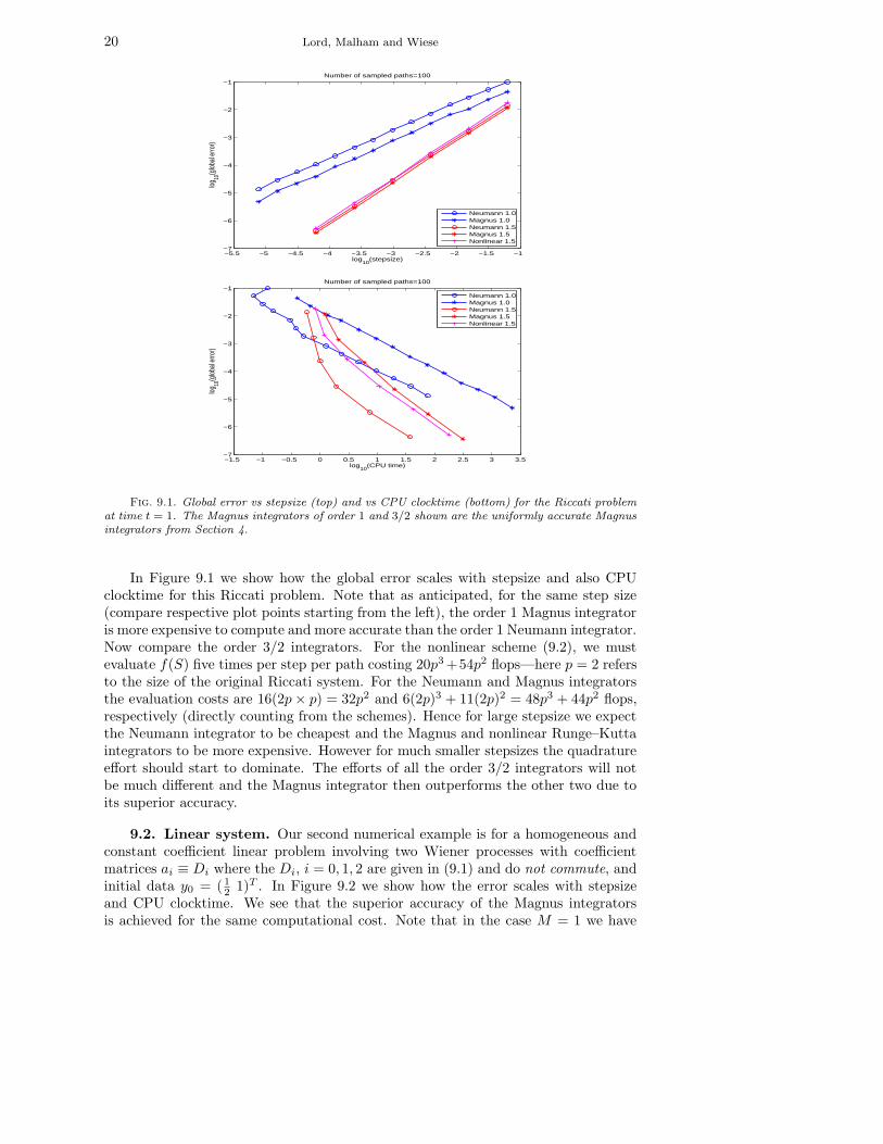
Fig. 9.1. Global error vs stepsize (top) and vs CPU clocktime (bottom) for the Riccati problemat time t = 1. The Magnus integrators of order 1 and 3/2 shown are the uniformly accurate Magnusintegrators from Section 4.

In Figure 9.1 we show how the global error scales with stepsize and also CPUclocktime for this Riccati problem. Note that as anticipated, for the same step size(compare respective plot points starting from the left), the order 1 Magnus integratoris more expensive to compute and more accurate than the order 1 Neumann integrator.Now compare the order 3/2 integrators. For the nonlinear scheme (9.2), we mustevaluate f(S) five times per step per path costing 20p3 +54p2 flops—here p = 2 refersto the size of the original Riccati system. For the Neumann and Magnus integratorsthe evaluation costs are 16(2p × p) = 32p2 and 6(2p)3 + 11(2p)2 = 48p3 + 44p2 flops,respectively (directly counting from the schemes). Hence for large stepsize we expectthe Neumann integrator to be cheapest and the Magnus and nonlinear Runge–Kuttaintegrators to be more expensive. However for much smaller stepsizes the quadratureeffort should start to dominate. The efforts of all the order 3/2 integrators will notbe much different and the Magnus integrator then outperforms the other two due toits superior accuracy.

9.2. Linear system. Our second numerical example is for a homogeneous andconstant coefficient linear problem involving two Wiener processes with coefficientmatrices ai ≡ Di where the Di, i = 0, 1, 2 are given in (9.1) and do not commute, andinitial data y0 = ( 1

2 1)T . In Figure 9.2 we show how the error scales with stepsizeand CPU clocktime. We see that the superior accuracy of the Magnus integratorsis achieved for the same computational cost. Note that in the case M = 1 we have


−3.5 −3 −2.5 −2 −1.5 −1 −0.5−2.5

−2

−1.5

−1

−0.5

0

0.5

1

log10

(stepsize)

log10

(glob

al er

ror)


Magnus 0.5Neumann 1.0Magnus 1.0Neumann 1.5Magnus 1.5

−1 −0.5 0 0.5 1 1.5 2−2.5

−2

−1.5

−1

−0.5

0

0.5

1

log10

(CPU time)

log10

(glob

al er

ror)



Fig. 9.2. Global error vs stepsize (top) and vs CPU clocktime (bottom) for the model problemat time t = 1 with 2 driving Wiener processes. The error corresponding to the largest step size takesthe shortest time to compute.

−3.5 −3 −2.5 −2 −1.5 −1 −0.5−2.5

−2

−1.5

−1

−0.5

0

0.5

1

log10

(stepsize)

log10

(glob

al er

ror)

Batch size=25; Number of batches=36

Magnus 1.0Magnus 1.5Confidence 90%Confidence 90%

Fig. 9.3. Confidence intervals for the global errors of the uniformly accurate Magnus integratorsfor the model problem at time t = 1 with 2 driving Wiener processes.

d = ` = 2. For the case when h ≤ hcr, when computational cost is dominated byquadrature effort, the relation between the global error E1 and computational cost Uis, ignoring Ueval and taking the logarithm,

log E1 ≈ log K1 − 12 logU .


−3.5 −3 −2.5 −2 −1.5 −1 −0.5−2

−1.5

−1

−0.5

0

0.5

1

1.5

log10

(stepsize)

log10

(glob

al er

ror)



−1.5 −1 −0.5 0 0.5 1 1.5 2−2

−1.5

−1

−0.5

0

0.5

1

1.5

log10

(CPU time)

log10

(glob

al er

ror)



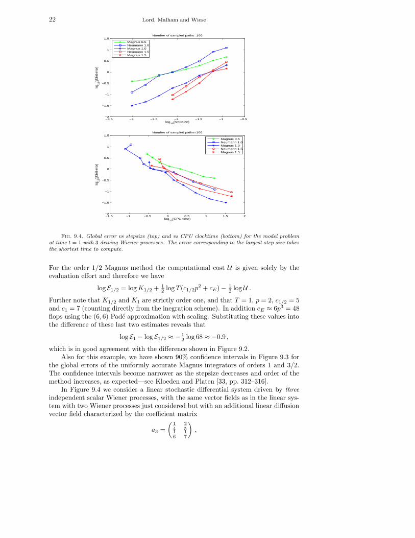
Fig. 9.4. Global error vs stepsize (top) and vs CPU clocktime (bottom) for the model problemat time t = 1 with 3 driving Wiener processes. The error corresponding to the largest step size takesthe shortest time to compute.

For the order 1/2 Magnus method the computational cost U is given solely by theevaluation effort and therefore we have

log E1/2 = log K1/2 + 12 log T (c1/2p

2 + cE) − 12 logU .

Further note that K1/2 and K1 are strictly order one, and that T = 1, p = 2, c1/2 = 5and c1 = 7 (counting directly from the inegration scheme). In addition cE ≈ 6p3 = 48flops using the (6, 6) Pade approximation with scaling. Substituting these values intothe difference of these last two estimates reveals that

log E1 − log E1/2 ≈ − 12 log 68 ≈ −0.9 ,

which is in good agreement with the difference shown in Figure 9.2.Also for this example, we have shown 90% confidence intervals in Figure 9.3 for

the global errors of the uniformly accurate Magnus integrators of orders 1 and 3/2.The confidence intervals become narrower as the stepsize decreases and order of themethod increases, as expected—see Kloeden and Platen [33, pp. 312–316].

In Figure 9.4 we consider a linear stochastic differential system driven by three

independent scalar Wiener processes, with the same vector fields as in the linear sys-tem with two Wiener processes just considered but with an additional linear diffusionvector field characterized by the coefficient matrix

a3 =

(14

25

16

17

),


which does not commute with a0, a1 or a2. Using Table 7.1 we would expect to seefor small stepsizes for the order 1 and 3/2 Magnus and Neumann methods, that theglobal error scales with the computational effort with exponent −1/2. This can beseen in Figure 9.4.

10. Concluding remarks. Our results can be extended to nonlinear stochasticdifferential equations. Consider a stochastic differential system governed by (d + 1)nonlinear autonomous vector fields Vi(y)—instead of the linear vector fields ‘ai(t)y’in (1.1)—and driven by a d-dimensional Wiener process (W 1, . . . ,W d). If we take thelogarithm of the stochastic Taylor series for the flow-map we obtain the exponentialLie series (see Chen [15] and Strichartz [54])

σt =

d∑

i=0

Ji(t)Vi +

d∑

j>i=0

12 (Jij − Jji)(t)[Vi, Vj ] + · · · .

Here [· , ·] is the Lie–Jacobi bracket on the Lie algebra of vectors fields defined on Rp.The solution yt of the system at time t > 0 is given by yt = exp σt◦y0 (see for exampleBen Arous [4] or Castell and Gaines [13, 14]). Across the interval [tn, tn+1] let σtn,tn+1

denote the exponential Lie series truncated to a given order, with multiple integralsapproximated by their expectations conditioned on intervening sample points. Then

ytn+1= exp

(σtn,tn+1

)◦ ytn

is an approximation to the exact solution ytn+1at the end point of the interval. The

truncated and conditioned exponential Lie series σtn,tn+1is itself an ordinary vector

field. Hence to compute ytn+1we solve the ordinary differential system

u′(τ) = σtn,tn+1◦ u(τ)

with u(0) = ytnacross the interval τ ∈ [0, 1] (see Castell and Gaines [13, 14]). If

we use a sufficiently accurate ordinary differential integrator commensurate with theorder of the truncation of the exponential Lie series then u(1) ≈ ytn+1

to that order.Hence the order 1/2 exponential Lie series integrator is more accurate than the

Euler–Maruyama method. Further in the case of commuting diffusion vector fields,the uniformly accurate exponential Lie series integrators of order 1 and 3/2 are moreaccurate than the stochastic Taylor approximations of the corresponding order. Thisgeneralization is discussed in Malham and Wiese [42]. An important future investiga-tion to justify the viability of these schemes would be the relation between global errorand computational cost, which must take into account the additional computationaleffort associated with the ordinary differential solver.

An important application for our results that we have in mind for the future arelarge order problems driven by a large number of Wiener processes. High-dimensionalproblems occur in many financial applications, for example in portfolio optimization orrisk management and in the context of option pricing when high-dimensional modelsare used, for example for the pricing of interest rate options or rainbow options.Large order problems also arise when numerically solving stochastic parabolic partialdifferential equation driven by a multiplicative noise term which is white noise intime and spatially smooth (see for example Lord and Shardlow [37]). Here we thinkof projecting the system onto a finite spatial basis set which results in a large systemof coupled ordinary stochastic differential equations each driven by a multiplicativenoise term. The high dimension d of the driving Wiener process will now be an


important factor in the computational cost for order M ≥ 1 as for example we willneed to simulate 1

2d(d−1) multiple integrals Jij ; though the results of Wiktorsson [58]suggest this can be improved upon. Krylov subspace methods for computing largematrix exponentials would be important for efficient implementation of our methodsfor this case (see Moler and Van Loan [47] and Sidje [52]).

Lastly, extensions of our work that we also intend to investigate further are: (1)implementing a variable step scheme following Gaines and Lyons [22], Lamba, Mat-tingly and Stuart [36], Burrage and Burrage [10] and Burrage, Burrage and Tian [9]—by using analytic expressions for the local truncation errors (see Aparicio, Malhamand Oliver [1]); (2) pricing path-dependent options; (3) deriving strong symplecticnumerical methods (see Milstein, Repin and Tretyakov [45]); and (4) constructing nu-merical methods based on the nonlinear Magnus expansions of Casas and Iserles [11].

Acknowledgments. We thank Kevin and Pamela Burrage, Sandy Davie, TerryLyons, Per-Christian Moan, Nigel Newton, Tony Shardlow, Josef Teichmann andMichael Tretyakov for stimulating discussions. The research in this paper was sup-ported by the EPSRC first grant number GR/S22134/01. A significant portion ofthis paper was completed while SJAM was visiting the Isaac Newton Institute in theSpring of 2007. We would also like to thank the anonymous referees for their veryhelpful comments and suggestions.

Appendix A. Neumann and Magnus integrators. We present Neumannand Magnus integrators up to global order 3/2 in the case of a d-dimensional Wienerprocess (W 1, . . . ,W d), and with constant coefficient matrices a0 and ai, i = 1, . . . , d.The Neumann expansion for the solution of the stochastic differential equation (1.1)over an interval [tn, tn+1], where tn = nh, is

yneutn,tn+1

≈(I + S1/2 + S1 + S3/2

)ytn

,

where (the indices i, j, k run over the values 1, . . . , d)

S1/2 = J0a0 +∑

i

Jiai +∑

i

Jiia2i ,

S1 =∑

i6=j

Jijaiaj ,

S3/2 =∑

i

(Ji0a0ai + J0iaia0) +∑

i,j,k

Jkjiaiajak

+∑

i

(J0iia2i a0 + Jii0a0a

2i ) +

∑

i,j

Jiijja2i a

2j + J00a

20 .

The corresponding approximation using the Magnus expansion is

ymagtn,tn+1

≈ exp(s1/2 + s1 + s3/2

)ytn

,


where, with [·, ·] as the matrix commutator,

s1/2 = J0a0 +∑

i

Jiai ,

s1 =∑

i<j

12 (Jji − Jij)[ai, aj ] ,

s3/2 =∑

i

12 (Ji0 − J0i)[a0, ai] +

∑

i6=j

(Jiij − 12JiJij + 1

12J2i Jj)[ai, [ai, aj ]]

+∑

i<j<k

((Jijk + 1

2JjJki + 12JkJij − 2

3JiJjJk)[ai, [aj , ak]]

+ (Jjik + 12JiJkj + 1

2JkJji − 23JiJjJk)[aj , [ai, ak]]

)

+∑

i

(Jii0 − 12JiJi0 + 1

12J2i J0)[ai, [ai, a0]] .

To obtain a numerical scheme of global order M using the Neumann or Magnusexpansion, we must use all the terms up to and including SM or sM , respectively.Leading order terms of order M + 1/2 with non-zero expectation can be replacedby their expectations (as detailed at the end of Section 3). Further, extending thesesolution series to the non-homogeneous and/or the non-constant coefficient case isstraightforward.

REFERENCES

[1] N. D. Aparicio, S. J. A. Malham, and M. Oliver, Numerical evaluation of the Evans functionby Magnus integration, BIT, 45 (2005), pp. 219–258.

[2] L. Arnold, Stochastic differential equations, Wiley, 1974.[3] R. Azencott, Formule de Taylor stochastique et developpement asymptotique d’integrales de

Feynman, Seminar on Probability XVI, Lecture Notes in Math., 921 (1982), Springer,pp. 237–285.

[4] G. Ben Arous, Flots et series de Taylor stochastiques, Probab. Theory Related Fields, 81(1989), pp. 29–77.

[5] O. Bobrovnytska and M. Schweizer, Mean-variance hedging and stochastic control: beyondthe Brownian setting, IEEE Trans. on Automatic Control, 49(3) (2004), pp. 396–408.

[6] F. Baudoin, An introduction to the geometry of stochastic flows, Imperial College Press, 2004.[7] P. M. Burrage, Runge–Kutta methods for stochastic differential equations, Ph.D. thesis, Uni-

versity of Queensland, 1999.[8] K. Burrage and P. M. Burrage, High strong order methods for non-commutative stochas-

tic ordinary differential equation systems and the Magnus formula, Phys. D, 133 (1999),pp. 34–48.

[9] K. Burrage, P. M. Burrage, and T. Tian, Numerical methods for strong solutions of stochas-tic differential equations: an overview, Proc. R. Soc. Lond. A, 460 (2004), pp. 373–402.

[10] P.M. Burrage and K. Burrage, A variable stepsize implementation for stochastic differentialequations, SIAM J. Sci. Comput., 24(3) (2002), pp. 848–864.

[11] F. Casas and A. Iserles, Explicit Magnus expansions for nonlinear equations, Technicalreport NA2005/05, DAMTP, University of Cambridge, 2005.

[12] F. Castell, Asymptotic expansion of stochastic flows, Probab. Theory Related Fields, 96(1993), pp. 225–239.

[13] F. Castell and J. Gaines, An efficient approximation method for stochastic differential equa-tions by means of the exponential Lie series, Math. Comput. Simulation, 38 (1995), pp. 13–19.

[14] , The ordinary differential equation approach to asymptotically efficient schemes forsolution of stochastic differential equations, Ann. Inst. H. Poincare Probab. Statist., 32(2)(1996), pp. 231–250.

[15] K. T. Chen, Integration of paths, geometric invariants and a generalized Baker–Hausdorffformula, Annals of Mathematics, 65(1) (1957), pp. 163–178.


[16] J. M. C. Clark and R. J. Cameron, The maximum rate of convergence of discrete approxi-mations for stochastic differential equations, in Lecture Notes in Control and InformationSciences, Vol. 25, 1980, pp. 162–171.

[17] A.B. Cruzeiro, P. Malliavin and A. Thalmaier, Geometrization of Monte-Carlo numericalanalysis of an elliptic operator: strong approximation, C. R. Acad. Sci. Paris, Ser. I, 338(2004), pp. 481–486.

[18] G. Freiling, A survey of nonsymmetric Riccati equations, Linear Algebra Appl., 351–352(2002), pp. 243–270.

[19] J. G. Gaines, The algebra of iterated stochastic integrals, Stochastics and stochastics reports,49(3–4) (1994), 169–179.

[20] , A basis for iterated stochastic integrals, Math. Comput. Simulation, 38 (1995), pp. 7–11.[21] J. G. Gaines and T. J. Lyons, Random generation of stochastic area integrals, SIAM J. Appl.

Math., 54(4) (1994), pp. 1132–1146.[22] , Variable step size control in the numerical solution of stochastic differential equations,

SIAM J. Appl. Math., 57(5) (1997), pp. 1455–1484.[23] I. I. Gihman, and A. V. Skorohod, The theory of stochastic processes III, Springer, 1979.[24] M.B. Giles, Multi-level Monte Carlo path simulation, OUCL, Report no. 06/03.[25] , Improved multilevel Monte Carlo convergence using the Milstein scheme, OUCL, Re-

port no. 06/22.[26] H. Gilsing and T. Shardlow, SDELab: stochastic differential equations with MATLAB,

MIMS EPrint: 2006.1, ISSN 1749-9097.[27] I. Gyongy, and G. Michaletzky, On Wong–Zakai approximations with δ-martingales, Proc.

R. Soc. Lond. A, 460 (2004), pp. 309–324.[28] D. J. Higham, An algorithmic introduction to numerical simulation of stochastic differential

equations, SIAM Rev., 43(3) (2001), pp. 525–546.[29] N. Hofmann, and T. Muller-Gronbach, On the global error of Ito–Taylor schemes for

strong approximation of scalar stochastic differential equations, J. Complexity, 20 (2004),pp. 732–752.

[30] A. Iserles, H. Z. Munthe-Kaas, S. P. Nørsett, and A. Zanna, Lie-group methods, ActaNumer., (2000), pp. 215–365.

[31] A. Iserles and A. Zanna, Efficient computation of the matrix exponential by generalized polardecompositions, SIAM J. Numer. Anal., 42(5) (2005), pp. 2218–2256.

[32] M. Kawski, The combinatorics of nonlinear controllability and noncommuting flows, Lecturesgiven at the Summer School on Mathematical Control Theory, Trieste, September 3–28,2001.

[33] P. E. Kloeden and E. Platen, Numerical solution of stochastic differential equations,Springer, 1999.

[34] M. Kohlmann and S. Tang, Multidimensional backward stochastic Riccati equations and ap-plications, SIAM J. Control Optim., 41(6) (2003), pp. 1696–1721.

[35] H. Kunita, On the representation of solutions of stochastic differential equations, LectureNotes in Math. 784, Springer–Verlag, 1980, pp. 282–304.

[36] H. Lamba, J.C. Mattingly and A.M. Stuart, An adaptive Euler-Maruyama scheme forSDEs: convergence and stability, IMA Journal of Numerical Analysis, 27 (2007), pp. 479–506.

[37] G.J. Lord and T. Shardlow, Post processing for stochastic parabolic partial differential equa-tions, SIAM J. Numer. Anal. 45(2) (2007), pp. 870–889.

[38] T. Lyons, Differential equations driven by rough signals, Rev. Mat. Iberoamericana, 14(2)(1998), pp. 215–310.

[39] T. Lyons and Z. Qian, System control and rough paths, Oxford University Press, 2002.[40] T. Lyons and N. Victoir, Cubature on Wiener space, Proc. R. Soc. Lond. A, 460 (2004),

pp. 169–198.[41] W. Magnus, On the exponential solution of differential equations for a linear operator, Comm.

Pure Appl. Math., 7 (1954), pp. 649–673.[42] S. J.A. Malham and A. Wiese, Stochastic Lie group integrators, SISC, accepted.[43] P. Malliavin, Stochastic analysis, Grundlehren der mathematischen Wissenschaften 313,

Springer, 1997.[44] G. N. Milstein, Numerical integration of stochastic differential equations, Mathematics and

its applications, Kluwer Academic Publishers, 1994.[45] G. N. Milstein, Yu. M. Repin, and M. V. Tretyakov, Numerical methods for stochastic

systems preserving symplectic structure, SIAM J. Numer. Anal., 40(4) (2002), pp. 1583–1604.

[46] T. Misawa, A Lie algebraic approach to numerical integration of stochastic differential equa-


tions, SIAM J. Sci. Comput., 23(3) (2001), pp. 866–890.[47] C. Moler and C. Van Loan, Nineteen dubious ways to compute the exponential of a matrix,

twenty-five years later, SIAM Rev., 45 (2003), pp. 3–49.[48] H.Z. Munthe–Kaas and W.M. Wright, On the Hopf algebraic structure of Lie group inte-

grators, preprint, 2006.[49] N. J. Newton, Asymptotically efficient Runge–Kutta methods for a class of Ito and

Stratonovich equations, SIAM J. Appl. Math., 51 (1991), pp. 542–567.[50] J. Schiff and S. Shnider, A natural approach to the numerical integration of Riccati differ-

ential equations, SIAM J. Numer. Anal., 36(5) (1999), pp. 1392–1413.[51] H. Schurz, A brief introduction to numerical analysis of (ordinary) stochastic differential

equations without tears, in Handbook of Stochastic Analysis and Applications, V. Laksh-mikantham and D. Kannan, eds., Marcel Dekker, 2002, pp. 237–359.

[52] R. B. Sidje, Expokit: a software package for computing matrix exponentials, ACM Transactionson Mathematical Software, 24(1) (1998), pp. 130–156.

[53] E.-M. Sipilainen, A pathwise view of solutions of stochastic differential equations, Ph.D. thesis,University of Edinburgh, 1993.

[54] R. S. Strichartz, The Campbell–Baker–Hausdorff–Dynkin formula and solutions of differen-tial equations, J. Funct. Anal., 72 (1987), pp. 320–345.

[55] D. M. Stump and J. M. Hill, On an infinite integral arising in the numerical integration ofstochastic differential equations, Proc. R. Soc. A, 461 (2005), pp. 397–413.

[56] H. J. Sussmann, Product expansions of exponential Lie series and the discretization of stochas-tic differential equations, in Stochastic Differential Systems, Stochastic Control Theory,and Applications, W. Fleming and J. Lions, eds., Springer IMA Series, Vol. 10, 1988,pp. 563–582.

[57] D. Talay, Simulation and numerical analysis of stochastic differential systems, in ProbabilisticMethods in Applied Physics, P. Kree and W. Wedig, eds., Lecture Notes in Physics, Vol.451, 1995, chap. 3, pp. 63–106.

[58] M. Wiktorsson, Joint characteristic function and simultaneous simulation of iterated Itointegrals for multiple independent Brownian motions, Ann. Appl. Probab., 11(2) (2001),pp. 470–487.

[59] E. Wong and M. Zakai, On the relation between ordinary differential and stochastic differ-ential equations, Internat. J. Engrg Sci., 3 (1965), pp. 213–229.

[60] Y. Yamato, Stochastic differential equations and nilpotent Lie algebras, Z. Wahrsch. Verw.Gebiete, 47(2) (1979), pp 213–229.

efficient strong integrators for linear stochastic systemssimonm/nsdes.pdf · efficient strong...

Documents