efficient stochastic galerkin methods for random …shen/pub/xiu_jcp08.pdf · efficient stochastic...

EFFICIENT STOCHASTIC GALERKIN METHODS FOR RANDOMDIFFUSION EQUATIONS

DONGBIN XIU∗ AND JIE SHEN†

Abstract. We discuss in this paper efficient solvers for stochastic diffusion equations in randommedia. We employ generalized polynomial chaos (gPC) expansion to express the solution in aconvergent series and obtain a set of deterministic equations for the expansion coefficients by Galerkinprojection. Although the resulting system of diffusion equations are coupled, we show that one canconstruct fast numerical methods to solve them in a decoupled fashion. The methods are basedon separation of the diagonal terms and off-diagonal terms in the matrix of the Galerkin system.We examine properties of this matrix and show that the proposed method is unconditionally stablefor unsteady problems and convergent for steady problems with a convergent rate independent ofdiscretization parameters. Numerical examples are provided, for both steady and unsteady randomdiffusions, to support the analysis.

Key words. Generalized polynomial chaos, stochastic Galerkin, random diffusion, uncertaintyquantification

1. Introduction. We discuss in this paper simulations of diffusion problemswith uncertainties. In general the uncertainties may enter through initial condi-tions, boundary conditions, or material properties. A representative example is flowthrough porous media, where the medium properties, e.g., permeability, are not pre-cisely known due to lack of measurements and their accuracy. Here we discuss fastalgorithms based on (generalized) polynomial chaos methods. Such methods have re-ceived considerable attention recently due to its efficiency in solving many stochasticproblems. The original polynomial chaos (PC) method was developed by R. Ghanemand co-workers, cf. [9]. It was inspired by the Wiener chaos expansion which employsHermite polynomials to represent Gaussian random processes [21]. Since its introduc-tion, the PC method has been applied to many problems, including random diffusion[8, 7, 17, 6]. Later the approach was extended to generalized polynomial chaos (gPC)where general orthogonal polynomials are adopted for improved representations ofmore general random processes [25]. With this extension different types of polynomi-als can be chosen to design efficient methods for problems with non-Gaussian inputs.Further extensions along this line include using piecewise basis functions to deal withdiscontinuity in random space more effectively [3, 11, 12, 20].

With PC/gPC serving as a complete basis to represent random processes, astochastic Galerkin projection can be used to transform the (stochastic) governingequations to a set of deterministic equations that can be readily discretized via stan-dard numerical techniques, see, for example, [1, 3, 4, 9, 11, 14, 25, 24, 26]. Oftensuch a procedure results in a set of coupled equations. For a stochastic diffusionequation this occurs when the diffusivity (or permeability, conductivity) is modeledas a random field. Here we employ the standard approach which models the ran-dom diffusivity field as a linear functional of finite number of (independent) randomvariables. The resulting deterministic equations from a Galerkin method are a set ofcoupled diffusion equations, which can be readily written in a vector/matrix form.We demonstrate that efficient algorithms can be constructed where only the diagonal

∗Department of Mathematics, Purdue University, West Lafayette, IN 47907([email protected]).

†Department of Mathematics, Purdue University, West Lafayette, IN 47907([email protected]).

1

2 DONGBIN XIU and JIE SHEN

terms are inverted whereas the off-diagonal terms are treated explicitly. This resultsin a mixed explicit/implicit scheme for unsteady diffusion and a Jacobi iteration forsteady diffusion. The important feature is that the system of equations are decoupledand existing methods for deterministic diffusion can be employed. Although suchapproaches have been used in practice, for both steady [24] and unsteady [27] randomdiffusions, their effectiveness has not been rigorously investigated. Here we show rig-orously that the stiffness matrix of the Galerkin system, in the case of identical betaor gamma distributions, is strictly diagonally dominant which allows us to show that(i) a first-order mixed explicit/implicit scheme for unsteady diffusion problems is un-conditionally stable; and (ii) the preconditioned CG method with a decoupled systemas a preconditioner, and the simple Jacobi iterative scheme, converge at a rate whichis independent of discretization parameters in the identical beta distribution case andonly weakly dependent on the discretization parameters in the gamma distributioncase.

It is also worth mentioning other means to decouple these random diffusion equa-tions.

One approach is to employ the double-orthogonal polynomials ([3]) which can beapplied when the random diffusivity is linear in terms of the input random variables(same as the case considered in this paper). The double-orthogonal polynomials,however, do not possess a hierarchical structure, and thus in multidimensional randomspaces one needs to use tensor products of the univariate polynomials. This canincrease computational cost drastically due to the fast growth in the number of basisfunctions.

Another approach is to use stochastic collocation methods (SC), which naturallyleads to decoupled system of equations. Earlier attempts typically utilize tensor prod-ucts of quadrature points, cf. [19]. Although it is still of high order, as shown in [2],the exponential growth of the number collocation points prevents its wide use in highdimensional random spaces. A more efficient alternative is to use Smolyak sparse grid([16]), which was proposed in [23] and shown to be highly effectively for stochasticproblems with high dimensional random inputs. In addition to solution statistics(e.g., mean and variance), a pseudo-spectral scheme can be employed to construct thecomplete gPC expansion [22].

Although the sparse grid based SC method is highly efficient, in general the num-ber of (uncoupled) deterministic equations is larger than that of (coupled) equationsfrom gPC Galerkin. This is particularly true at higher orders, as in large randomdimensions the number of sparse grid SC equations scales as ∼ 2P times the numberof gPC Galerkin equations, where P is the order of approximation. Although adaptivechoice of collocation nodes, based on solution property, can be made to reduce thecomputational cost [5], the number of equations can still be significantly higher thanthat of gPC Galerkin method, especially at high random dimensions and/or high or-der expansions. Therefore it is important to develop efficient algorithms for the gPCGalerkin system which, albeit coupled, involves the “least” number of equations.

This paper is organized as follows. In Section 2 we formulate the random diffusionproblem, for both steady and unsteady state problems. The gPC Galerkin methodis presented in Section 3 where we prove a few important properties of the matrixstructure. A mixed explicit/implicit algorithm is presented in Section 4, and itsconvergence and stability are established. We finally present numerical examples inSection 5.

TIME INTEGRATION OF RANDOM DIFFUSION 3

2. Governing Equations. We consider a time-dependent stochastic diffusionequation

∂u(t, x, y)∂t

= ∇x · (κ(x, y)∇xu(t, x, y)) + f(t, x, y), x ∈ Ω, t ∈ (0, T ];

u(0, x, y) = u0(x, y), u(t, ·, y)|∂Ω = 0,(2.1)

and its steady state counterpart

−∇x · (κ(x, y)∇xu(x, y)) = f(x, y), x ∈ Ω; u(·, y)|∂Ω = 0, (2.2)

where x = (x1, . . . , xd)T ∈ Ω ⊂ Rd, d = 1, 2, 3, are the spatial coordinates, andy = (y1, . . . , yN ) ∈ RN , N ≥ 1, is a random vector with independent and identicallydistributed components.

We assume that the random diffusivity field takes a form

κ(x, y) = κ0(x) +N∑

i=1

κi(x)yi, (2.3)

where κi(x)Ni=0 are fixed functions with κ0(x) > 0, ∀x. Alternatively (2.3) can be

written as

κ(x, y) =N∑

i=0

κi(x)yi, (2.4)

where y0 = 1.For well-posedness we require

κ(x, y) ≥ κmin > 0, ∀x ∈ Ω, y ∈ RN . (2.5)

Such a requirement obviously excludes random vector y that is unbounded from below,e.g., Gaussian distribution. Throughout this paper we will only consider randomvariables that are bounded from below.

3. GPC Galerkin Method.

3.1. GPC Galerkin Equations. The P th-order, gPC approximations of u(t, x, y)and f(t, x, y) are

u(t, x, y) ≈M∑

m=1

vm(t, x)Φm(y), f(t, x, y) ≈M∑

m=1

fm(t, x)Φm(y), (3.1)

where M =(N+P

N

), Φm(y) are N -variate orthonormal polynomials of degree up to

P . They are constructed as products of a sequence of univariate polynomials in eachdirection of yi, i = 1, . . . , N , i.e.,

Φm(y) = φm1(y1) · · ·φmN (yN ), m1 + · · ·+ mN ≤ P, (3.2)

where mi is the order of the univariate polynomials of φ(yi) in the yi direction for1 ≤ i ≤ N . These univariate polynomials are orthonormal (upon proper scaling), i.e,

∫φj(yi)φk(yi)ρi(yi)dyi = δjk, 1 ≤ i ≤ N, (3.3)


where δjk is the Kronecker delta function and ρi(yi) is the probability distributionfunction for random variable yi. The type of the polynomials φ(yi) is determinedby the distribution of yi. For example, Hermite polynomials are better suited forGaussian distribution (the original PC expansion [9]), Jacobi polynomials are betterfor beta distribution, etc. For detailed discussion, see [25]. The polynomials alsosatisfy a three-term recurrence relation:

zφk(z) = akφk+1(z) + bkφk(z) + ckφk−1(z), k ≥ 1, (3.4)

with φ0 = 1, φ−1 = 0.For the N -variate basis polynomials Φm(y), each index 1 ≤ m ≤ M corresponds

to a unique sequence m1, . . . ,mN , and they are also orthonormal

E[Φm(y)Φn(y)] =∫

Φm(y)Φn(y)ρ(y)dy = δmn, (3.5)

where ρ(y) = ΠNi=1ρi(yi).

Upon substituting (2.3) and the approximation (3.1) into the governing equation(2.1) and projecting the resulting equation onto the subspace spanned by the first MgPC basis polynomials, we obtain for all k = 1, . . . , M ,

∂vk

∂t(t, x) =

N∑

i=0

M∑

j=1

∇x · (κi(x)∇xvj)eijk + fk(t, x)

=M∑

j=1

∇x · (ajk(x)∇xvj) + fk(t, x), (3.6)

where

eijk = E[yiΦjΦk] =∫

yiΦj(y)Φk(y)ρ(y)dy, 0 ≤ i ≤ N, 1 ≤ j, k ≤ M,

ajk(x) =N∑

i=0

κi(x)eijk, 1 ≤ j, k ≤ M. (3.7)

Alternatively, we can write

ajk(x) = E [κΦjΦk] =∫

κ(x, y)Φj(y)Φk(y)ρ(y)dy, 1 ≤ j, k ≤ M. (3.8)

Note this is a more general expression which is valid for general random diffusivitymodels not restricted to the linear form in y (2.3).

Let us denote v = (v1, · · · , vM )T , f = (f1, · · · , fM )T and A(x) = (ajk)1≤j,k≤M .By definition, A = AT is symmetric. The gPC Galerkin equations (3.6) can bewritten as

∂v∂t

(t, x) = ∇x · [A(x)∇xv] + f , (t, x) ∈ (0, T ]× Ω,

v(0, x) = v0(x), v|∂Ω = 0.(3.9)

This is a coupled system of diffusion equations, where v0(x) is the gPC expansioncoefficient vector obtained by expressing the initial condition of (2.1) in the form of(3.1).


Similarly, by removing the time variable t from the above discussion, we find thatthe gPC Galerkin approximation to (2.2) is:

−∇x · [A(x)∇xv] = f , x ∈ Ω; v|∂Ω = 0. (3.10)

This is a coupled system of elliptic equations.

3.2. Properties of the matrix A(x). The following results are based on theconditions described above, i.e.,

• Diffusivity field κ(x, y) is constructed by (2.4) and satisfies (2.5);• The N -variate polynomials basis functions used in the solution expansion

(3.1) are constructed via (3.2) and are orthonormal as in (3.5);• The univariate polynomials in the constructions of (3.2) are orthonormal as

in (3.3) and satisfy the three-term recurrence relation (3.4);• The gPC Galerkin approximation of problem (2.1) (resp. (2.2)) results in a

system of equation (3.9) (resp. (3.10)), where the symmetric matrix A(x) isdefined by (3.7).

Under these conditions, we haveTheorem 3.1. The matrix A(x) is positive definite for any x ∈ Ω, following

assumption (2.5).

Proof. Let b = (b1, · · · , bM )T be an arbitrary non-zero real vector, and b(y) =∑Mj=1 bjΦj(y) be a random variable constructed by the b vector. By using the defi-

nition of ajk(x) in (3.8), we immediately have, for any x ∈ Ω,

bT A(x)b =M∑

j=1

M∑

k=1

bjajk(x)bk

=M∑

j=1

M∑

k=1

bj

∫κ(x, y)Φj(y)Φk(y)ρ(y)dybk

=∫

κ(x, y)b2(y)ρ(y)dy

> 0,

where the last inequality follows from (2.5). Note this result is valid for general formof diffusivity (3.8) and is not restricted to the linear form (2.4), as it only assumes(2.5).

Lemma 3.2. Each row of A(x) has at most (2N + 1) non-zero entries.Proof. From the definition of the matrix A(x) in (3.7), we obtain, for 1 ≤ j, k ≤

M ,

ajk(x) = κ0(x)e0jk +N∑

i=1

κi(x)eijk

= κ0(x)δjk +N∑

i=1

κi(x)E[yiΦj(y)Φk(y)] (3.11)


The first term in the above expression goes into the diagonal entries of matrixA(x). By using the three-term recurrence relation (3.4), the second term becomes

E[yiΦj(y)Φk(y)] = E [yiφj1(y1) · · ·φjN(yN )φk1(y1) · · ·φkN

(yN )]

=∫· · ·

∫φj1(y1) · · · [aji

φji+1(yi) + bjiφji

(yi) + cjiφji−1(yi)] · · ·φjN

(yN )

·φk1(y1) · · ·φkN(yN )

N∏

i=1

ρi(yi)dy1 · · · dyN

= δj1,k1 · · · (ajiδji+1,ki + bjiδji,ki + cjiδji−1,ki) · · · δjN ,kN

= ajiE[Φji+(y)Φk(y)] + bji

E[Φj(y)Φk(y)] + cjiE[Φji−(y)Φk(y)]

= ajiδji+,k + bji

δj,k + cjiδji−,k, (3.12)

where

Φji+(y) = φj1(y1) · · ·φji+1(yi) · · ·φjN(yN ),

Φji−(y) = φj1(y1) · · ·φji−1(yi) · · ·φjN (yN ).

That is, the multivariate polynomial Φji+(y) (resp. Φji−(y)) is the same as Φj(y) ex-cept the order of its univariate polynomial component in the ith direction is perturbedby +1 (resp. −1).

The above derivation shows that for any row of A(x), each term in the N -termsummation of (3.11) has one contribution to the diagonal term, and two non-zerocontributions to the off-diagonal entries. Therefore the maximum of number of non-zero entries in each row of A(x) is (2N + 1).

Following the above derivation the diagonal terms of A are

ajj(x) = κ0(x) +N∑

i=1

κi(x)bji , 1 ≤ j ≤ M, (3.13)

where ji are the orders of the univariate polynomials in the directions of yi for 1 ≤i ≤ N of the N -variate polynomial basis Φj(y).

Lemma 3.3. Assume that the random variables yi, 1 ≤ i ≤ N , in (2.4) haveeither an identical beta distribution in (−1, 1) with ρ(yi) ∼ (1 − yi)α(1 + yi)α, or agamma distribution in (0, +∞) with ρ(yi) ∼ yα

i e−yi , where α > −1 and the scalingconstants are omitted. Then, the matrices A(x) derived via the corresponding gPCbasis are strictly diagonal dominant ∀x ∈ Ω. More precisely, we have

ajj(x) ≥ κmin +M∑

k=1,k 6=j

|ajk(x)| , 1 ≤ j ≤ M, ∀x ∈ Ω. (3.14)

Proof. We start with the beta distribution case where ρ(yi) ∼ (1− yi)α(1 + yi)α

which corresponds to the ultra-spherical polynomials ([25]). Since yi ∈ [−1, 1], takingyi = ±1 in (2.3), the condition (2.5) immediately implies that

κ0(x) ≥ κmin +N∑

i=1

|κi(x)| , ∀x ∈ Ω. (3.15)


We recall that for ultra-spherical polynomials, the coefficients in their three-termrecurrence satisfy (c.f., [18])

bm = 0, am, cm > 0, am + cm = 1, m ≥ 1.

Therefore, we derive from Lemma 3.2, (3.11) and (3.12) that the sum of off-diagonalterms satisfy

M∑

k=1,k 6=j

|ajk(x)| =N∑

i=1

|κi(x)| (aji + cji) =N∑

i=1

|κi(x)| .

On the other hand, we derive from (3.13) that

ajj(x) = κ0(x) 1 ≤ j ≤ M. (3.16)

Then, the inequality (3.14) follows from the above and (3.15).Consider now the case of gamma distribution with ρ(yi) ∼ yα

i e−yi which corre-sponds to generalized Laguerre polynomials ([25]). Since y ∈ [0,∞)N , letting y = 0and y →∞ in (2.3) together with (2.5) leads to

κ0(x) ≥ κmin, ∀x ∈ Ω;κi(x) > 0, 1 ≤ i ≤ N, ∀x ∈ Ω.

(3.17)

We recall that for generalized Laguerre polynomials, the coefficients in their three-term recurrence relation are (c.f., [18])

am = −(m + 1), bm = 2m + α + 1, cm = −(m + α). (3.18)

Hence, we have bm > 0,∀m, (since α > −1) and am +cm = −bm. We then derive fromLemma 3.2, (3.11), (3.12), and the above relations that the sum of the off-diagonalterms satisfies

M∑

k=1,k 6=j

|ajk(x)| =N∑

i=1

|κi(x) (aji + cji)| =N∑

i=1

κi(x)bji .

We conclude from the above, (3.17) and (3.13).Remark 3.1. It is an open question whether the above lemma holds for general

beta distributions in (−1, 1) with ρ(yi) ∼ (1−yi)α(1+yi)β, α 6= β, α, β > −1, althoughthe numerical results in Section 5 (cf. Fig. 5.4) appear to indicate that the lemmaholds for the general beta distributions as well.

We now establish a simple result which plays an important role in designingefficient schemes for (3.9) and (3.10).

Lemma 3.4. Assume that a symmetric M ×M matrix A = (aij) satisfies

ajj ≥ κ +M∑

k=1,k 6=j

|ajk| , j = 1, 2, · · · ,M, (3.19)

and set

D = diag(A), A = D + S. (3.20)


Then,

2|uT Sv| ≤ ut(D− κI)u + vt(D− κI)v, ∀u,v ∈ RM ; (3.21)

and

κuT u ≤ uT Au ≤ uT (2D− κI)u, ∀u ∈ RM . (3.22)

Proof.For any u,v ∈ RM , using (3.19) and the fact that sij = sji, we find

2∣∣uT Sv

∣∣ = 2

∣∣∣∣∣∣

M∑

i,j=1

sijuivj

∣∣∣∣∣∣≤

M∑

i,j=1

(|sij |u2i + |sij | v2

j )

≤M∑

i=1

(aii − κ)u2i +

M∑

j=1

(ajj − κ)v2j

which is exactly (3.21).Now take v = u in (3.21), we find

uT Au = uT Du + uT Su ≤ uT Du + uT (D− κI)u = uT (2D− κI)u,

and

uT Au ≥ uT Du−∣∣uT Su

∣∣ ≥ uT Du− uT (D− κI)u = κuT u.

4. Numerical approaches. A disadvantage of the stochastic Galerkin method,as opposed to the stochastic collocation method, is that it leads to a coupled parabolicsystem (3.9) or elliptic system (3.10) for all components of v. We shall show belowthat by taking advantage of the diagonal dominance of A, one can efficiently solve thesystems (3.9) and (3.10) as decoupled equations, similar to the stochastic collocationapproach.

4.1. Time dependent problem (3.9). To avoid solving a coupled elliptic sys-tem at each time step, we propose a mixed explicit/implicit scheme for time integra-tion of (3.9). More precisely, we write

A(x) = D(x) + S(x), (4.1)

where D(x) is the diagonal part and S(x) the off-diagonal part, and treat the diagonalterms in (3.9) implicitly and the off-diagonal ones explicitly. For example, a mixedEuler explicit/implicit scheme takes the following form

vn+1 − vn

∆t−∇x · [D(x)∇xvn+1] = ∇x · [S(x)∇xvn] + fn+1, (4.2)

where vn = v(tn, x), fn+1 =∫ tn+1

tnf(t, x)dt and ∆t is the time step. Note that at

each time step, the above scheme requires solving only a sequence of M decoupledelliptic equations.


Theorem 4.1. Under the conditions in Lemma 3.3, the scheme (4.2) is uncon-ditionally stable, and

‖vk‖2 +k−1∑

j=0

‖vj − vj−1‖2 + κmin∆t‖∇xvj‖2

≤ C(‖v0‖2 + ∆t(D(x)∇xv0,∇xv0) + ‖f‖2L2([0,T ]×Ω)

), ∀k ≤ [T/∆t],

where ‖ · ‖2 =∫Ω‖ · ‖2l2dx.

Proof. Taking the inner product, with respect to x in L2(Ω), of (4.2) with2∆tvn+1 and integration by parts, using the identity 2(a− b, a) = |a|2−|b|2 + |a− b|2and (3.21), we find

‖vn+1‖2 − ‖vn‖2 + ‖vn+1 − vn‖2 + 2∆t(D(x)∇xvn+1,∇xvn+1)

= 2∆t(S(x)∇xvn,∇xvn+1) + 2∆t(fn+1,vn+1)

≤ ∆t(D− κminI)∇xvn,∇xvn) + ∆t(D− κminI)∇xvn+1,∇xvn+1)

+ ∆t‖fn+1‖2 + ∆t‖vn+1‖2.

Summing up the above inequality for n = 0 to n = k − 1 and dropping some unnec-essary positive terms, we find

‖vk‖2 +k−1∑

j=0

‖vj − vj−1‖2 + κmin∆t(‖∇xvj‖2 + ‖∇xvj+1‖2)

≤ ‖v0‖2 + ∆t(D(x)∇xv0,∇xv0) + ‖f‖2L2([0,T ]×Ω).

Scheme (4.2) is only first order in time. For higher temporal accuracy, a high-orderbackward differentiation formula can be used ([27])

γ0vn+1(x)−∑J−1q=0 αqvn−q(x)

∆t−∇x·[D(x)∇xvn+1] =

J−1∑q=0

βq∇x·[S(x)∇xvn−q]+fn+1,

(4.3)where J is the order of accuracy in time. The coefficients in the scheme are listed intable 4.1 for different temporal orders. It is unlikely that the above scheme will beunconditionally stable for J ≥ 2, but one can expect the scheme with J ≥ 2 to bestable under mild stability constraints.

Coefficient 1st order 2nd order 3rd orderγ0 1 3/2 11/6α0 1 2 3α1 0 -1/2 -3/2α2 0 0 1/3β0 1 2 3β1 0 -1 -3β2 0 0 1

Table 4.1Coefficients in the mixed explicit-implicit integration (4.3) (see, for example, [10], chapter 8).


Remark 4.1. In the decoupled system of equations (4.2) (or (4.3)), the explicitevaluation of ∇x · [S∇xv] can be accomplished by a matrix-vector product operation.Since A(x) is symmetric and only has (2N + 1) nonzero entries per row (see Lemma3.2) for each component of the explicit term, the dominant computational cost is theevaluation of (N +1) products which depends only on the random dimensionality N .

4.2. Steady state problem (3.10). For the steady state problem (3.10), weshall treat the identical beta distributions and gamma distributions separately.

For the identical beta distributions, we assume

κ0(x) ≤ κmax < +∞, ∀x. (4.4)

Using the same notations as in Lemma 3.4 and taking y = 0 in (2.3), we immediatelyderive from (4.4) and (3.16) that

uT Du = κ0(x)uT u ≤ κmaxuT u, ∀x ∈ Ω, u ∈ RM . (4.5)

We then derive from the above and (3.22) that

κminuT u ≤ uT A(x)u ≤ (2κmax − κmin)uT u, ∀x ∈ Ω, u ∈ RM . (4.6)

Let us consider now (3.10) and define a bilinear form

a(u,v) = (A(x)∇xu,∇xv), ∀u,v ∈ H10 (Ω)M . (4.7)

Then, we derive from (4.6) that

κmin(∇xu,∇xu) ≤ a(u,v) ≤ (2κmax − κmin)(∇xu,∇xu), ∀u ∈ H10 (Ω)M . (4.8)

This inequality indicates that for the case with identical beta distributions thebilinear form associated with the Laplace operator (∇xu,∇xu) is an optimal pre-conditioner for a(u,v). In particular, this implies that the convergence rate of thepreconditioned conjugate gradient (PCG) iteration, using the Laplace operator (withhomogeneous Dirichlet boundary conditions) as a preconditioner, will be independentof discretization parameters.

Now we consider the case of gamma distributions. We shall make an additionalassumption (which is not restrictive from a practical point of view):

κ0(x), κi(x) (i = 1, · · · , N) ≤ κmax < +∞, ∀x. (4.9)

Then, we derive from (4.9), (3.13), bm = 2m + α + 1 and m1 + · · ·+ mN ≤ P that

ajj(x) ≤ κmax + κmax

N∑

i=1

(2ji + α + 1)

= κmax + κmax

(2

N∑

i=1

ji + N(α + 1)

)≤ (2P + N(α + 1) + 1)κmax.

(4.10)

where N is the dimension of the random space and P is the highest polynomial order.Therefore, the same argument as above leads to

κmin(∇xu,∇xu) ≤ a(u,v) ≤ (2(2P +N(α+1)+1)κmax−κmin)(∇xu,∇xu). (4.11)


This result indicates that, in the case of gamma distributions, the convergencerate of the PCG iteration will depend on N and P weakly. This is consistent withthe numerical results in Section 5.

By taking into account (3.21), it is also easy to see that the above conclusion alsoholds for the simple Jacobi iteration

−∇x · [D(x)∇xvi+1] = ∇x · [S(x)∇xvi] + f , (4.12)

which, in the case of identical beta distributions, is equivalent to

−∇x · [κ0(x)∇xvi+1] = ∇x · [(A(x)− κ0(x))∇xvi] + f . (4.13)

Notice that only one matrix inversion is needed for all components of v. However,in the case of gamma distributions, (4.12) with full diagonal terms involves a matrixinversion for each component of v. The numerical results in Section 5 (cf., Fig. 5.7)indicate that the iterative scheme (4.12) with full diagonal terms is much more robustthan the scheme (4.13).

4.3. Advection-diffusion Problem. The algorithm presented here can be ex-tended to stochastic advection-diffusion problem in a straightforward manner. Let usconsider, for example, the following equation

ut + c(x) · ∇xu = ∇x · (κ(x, y)∇xu) + f(t, x, y), x ∈ Ω, t ∈ (0, T ], y ∈ RN , (4.14)

where c(x) is a deterministic advection velocity field, and proper initial and boundaryconditions are imposed. We remark that the case of random advection velocity hasbeen discussed extensively in literature, see, for example, [9]. Using the same notationsand approach from above, the first-order (in time) mixed explicit/implicit scheme canbe written as

vn+1 − vn

∆t−∇x · [D(x)∇xvn+1] = −c · ∇vn +∇x · [S(x)∇xvn] + fn+1. (4.15)

Similarly, a higher-order temporal scheme can be written in a similar fashion as thatof (4.3),

1∆t

[γ0vn+1(x)−∑J−1

q=0 αqvn−q(x)]−∇x · [D(x)∇xvn+1]

= fn+1 +∑J−1

q=0 βq (−c · ∇vn−q +∇x · [S(x)∇xvn−q]) ,(4.16)

where the coefficients α, β are tabulated in Table 4.1.

5. Numerical Examples. In this section we present numerical examples tosupport the analysis. The focus is on the discretization of random spaces and theconvergence properties of the proposed schemes. Therefore all numerical examples arein one-dimensional physical space. Extensions to two and three dimensional spacesare straightforward. We also remark that the decoupling methods discussed here havebeen applied in practice, cf., [24, 27], where extensive numerical tests were conductedfor problems involving complex geometry and large random perturbation.

5.1. Steady State Problem. We first consider the following problem in onespatial dimension (d = 1) and N (> 1) random dimensions.

− ∂

∂x

[κ(x, y)

∂u

∂x(x, y)

]= f, (x, y) ∈ (0, 1)× RN , (5.1)


with forcing term f = const and boundary conditions

u(0, y) = 0, u(1, y) = 0, y ∈ RN .

We assume that the random diffusivity has the form

κ(x, y) = 1 + σ

N∑

k=1

1k2π2

cos(2πkx)yk, (5.2)

where y = (y1, . . . , yN ) is a random vector with independent and identically dis-tributed components. The form of (5.2) is similar to those obtained from a Karhunen-Loeve expansion ([13]) with eigenvalues delaying as 1/k4. Here we employ (5.2) inorder to eliminate the errors associated with a numerical Karhunen-Loeve solver andto keep the random diffusivity strictly positive because the series converges as N →∞.The spatial discretization is a p-type spectral element with high-order modal expan-sions utilizing Jacobi polynomials [10]. In all of the following computations, suffi-ciently high order expansions are employed such that the spatial errors are negligible.

5.1.1. Random inputs with beta distribution. We first examine the casewhen the random variables in y have bounded support. In particular, we first set yas uniform random vector in (−1, 1)N In the first example we set N = 2 and σ = 1in (5.2). Since analytical solution is not readily available, we employ a well-resolvedsolution with gPC order P = 8 as the “exact” solution and examine convergence oferrors at lower order gPC expansions. In Figure 5.1 the errors in standard deviation(STD), with L2 norm in x, are shown. Fast (exponential) error convergence is observedas the order of gPC expansion is increased, before machine accuracy is reached. Forthe iterative solver (4.12), its convergence criterion is set at 1·10−10. Convergence canbe reached in 6 steps of iterations, as shown in Figure 5.2, for all orders of gPC solvers.More importantly, the convergence rate of the Jacobi iterative solvers is independentto the gPC expansion order.

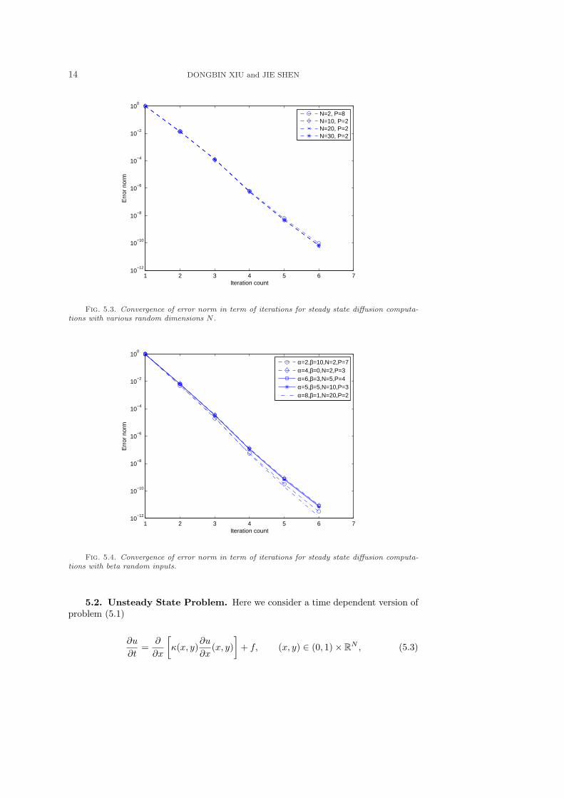
Next we vary the dimensionality of the random inputs, i.e., N in (5.2). Com-putations are conducted for random dimensions as high as N = 30, which results inM = 496 gPC expansion terms at second-order (P = 2). Numerical experiments in-dicate that the convergence rate of the Jacobi iteration is independent of the randomdimension N , as shown in Figure 5.3.

Even though the diagonal dominance proof in Theorem 3.3 applies only to thesymmetric beta distributions with α = β, we examine the convergence propertiesnumerically for general beta distribution with α 6= β. The results are plotted inFigure 5.4, for various combinations of α, β, dimensionality N , and gPC order P .It can be seen that the convergence rate of the iterative solver is insensitive of theparameter values.

5.1.2. Random inputs with gamma distribution. Next we assume ykNk=1

in the diffusivity model (5.2) have a gamma distribution with α = 1 (see Lemma 3.3)and examine the performance of the iterative scheme (4.12). To ensure positivenessof the diffusivity we slightly change the form from (5.2) to

κ(x, y) = 1 + σ

N∑

k=1

1k2π2

[1 + cos(2πkx)]yk.

The results are shown in Figure 5.5 with N = 2. It is clear that the convergenceis again fast and its rate appears to be insensitive to the order of gPC expansion athigher orders.


1 2 3 4 5 6 710

−18

10−16

10−14

10−12

10−10

10−8

10−6

10−4

Expansion Order

Err

or in

ST

D

Fig. 5.1. Convergence of error in standard deviation (STD) for steady state diffusion compu-tation with N = 2, σ = 1.

1 2 3 4 5 6 710

−12

10−10

10−8

10−6

10−4

10−2

100

Iteration count

Err

or n

orm

1st order4th order8th order

Fig. 5.2. Convergence of error norm in term of iterations for the steady state diffusion com-putation with N = 2, σ = 1.

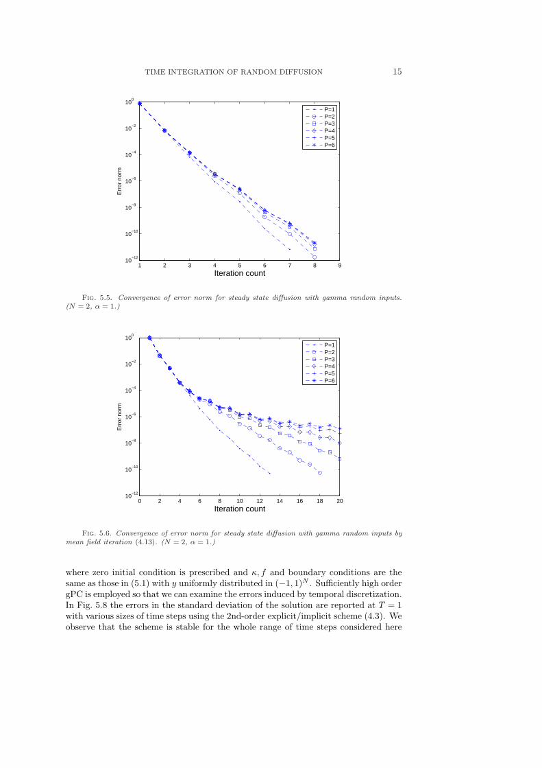
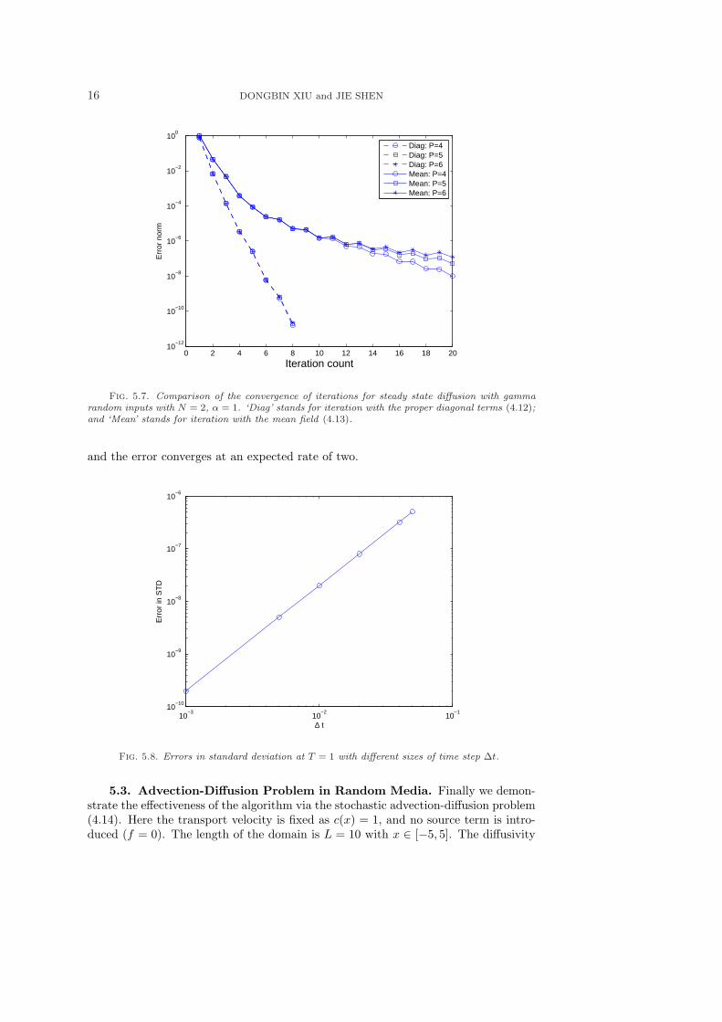
On the contrary, if one employs the iterative scheme based on the zero-th mode ofthe diffusivity field in (4.13), then the convergence becomes sensitive to the expansionorder. This is shown in Figure 5.6, where for higher order expansions the convergencerate deteriorates. The comparison of the two iterative schemes is in Figure 5.7, whereit is clear that the proper scheme (4.12) is more robust and accurate than the iterationbased on mean field (4.13).


1 2 3 4 5 6 710

−12

10−10

10−8

10−6

10−4

10−2

100

Iteration count

Err

or n

orm

N=2, P=8N=10, P=2N=20, P=2N=30, P=2

Fig. 5.3. Convergence of error norm in term of iterations for steady state diffusion computa-tions with various random dimensions N .

1 2 3 4 5 6 710

−12

10−10

10−8

10−6

10−4

10−2

100

Iteration count

Err

or n

orm

α=2,β=10,N=2,P=7α=4,β=0,N=2,P=3α=6,β=3,N=5,P=4α=5,β=5,N=10,P=3α=8,β=1,N=20,P=2

Fig. 5.4. Convergence of error norm in term of iterations for steady state diffusion computa-tions with beta random inputs.

5.2. Unsteady State Problem. Here we consider a time dependent version ofproblem (5.1)

∂u

∂t=

∂

∂x

[κ(x, y)

∂u

∂x(x, y)

]+ f, (x, y) ∈ (0, 1)× RN , (5.3)


1 2 3 4 5 6 7 8 910

−12

10−10

10−8

10−6

10−4

10−2

100

Iteration count

Err

or n

orm

P=1P=2P=3P=4P=5P=6

Fig. 5.5. Convergence of error norm for steady state diffusion with gamma random inputs.(N = 2, α = 1.)

0 2 4 6 8 10 12 14 16 18 2010

−12

10−10

10−8

10−6

10−4

10−2

100

Iteration count

Err

or n

orm

P=1P=2P=3P=4P=5P=6

Fig. 5.6. Convergence of error norm for steady state diffusion with gamma random inputs bymean field iteration (4.13). (N = 2, α = 1.)

where zero initial condition is prescribed and κ, f and boundary conditions are thesame as those in (5.1) with y uniformly distributed in (−1, 1)N . Sufficiently high ordergPC is employed so that we can examine the errors induced by temporal discretization.In Fig. 5.8 the errors in the standard deviation of the solution are reported at T = 1with various sizes of time steps using the 2nd-order explicit/implicit scheme (4.3). Weobserve that the scheme is stable for the whole range of time steps considered here


0 2 4 6 8 10 12 14 16 18 2010

−12

10−10

10−8

10−6

10−4

10−2

100

Iteration count

Err

or n

orm

Diag: P=4Diag: P=5Diag: P=6Mean: P=4Mean: P=5Mean: P=6

Fig. 5.7. Comparison of the convergence of iterations for steady state diffusion with gammarandom inputs with N = 2, α = 1. ‘Diag’ stands for iteration with the proper diagonal terms (4.12);and ‘Mean’ stands for iteration with the mean field (4.13).

and the error converges at an expected rate of two.

10−3

10−2

10−1

10−10

10−9

10−8

10−7

10−6

∆ t

Err

or in

ST

D

Fig. 5.8. Errors in standard deviation at T = 1 with different sizes of time step ∆t.

5.3. Advection-Diffusion Problem in Random Media. Finally we demon-strate the effectiveness of the algorithm via the stochastic advection-diffusion problem(4.14). Here the transport velocity is fixed as c(x) = 1, and no source term is intro-duced (f = 0). The length of the domain is L = 10 with x ∈ [−5, 5]. The diffusivity


field is modeled as

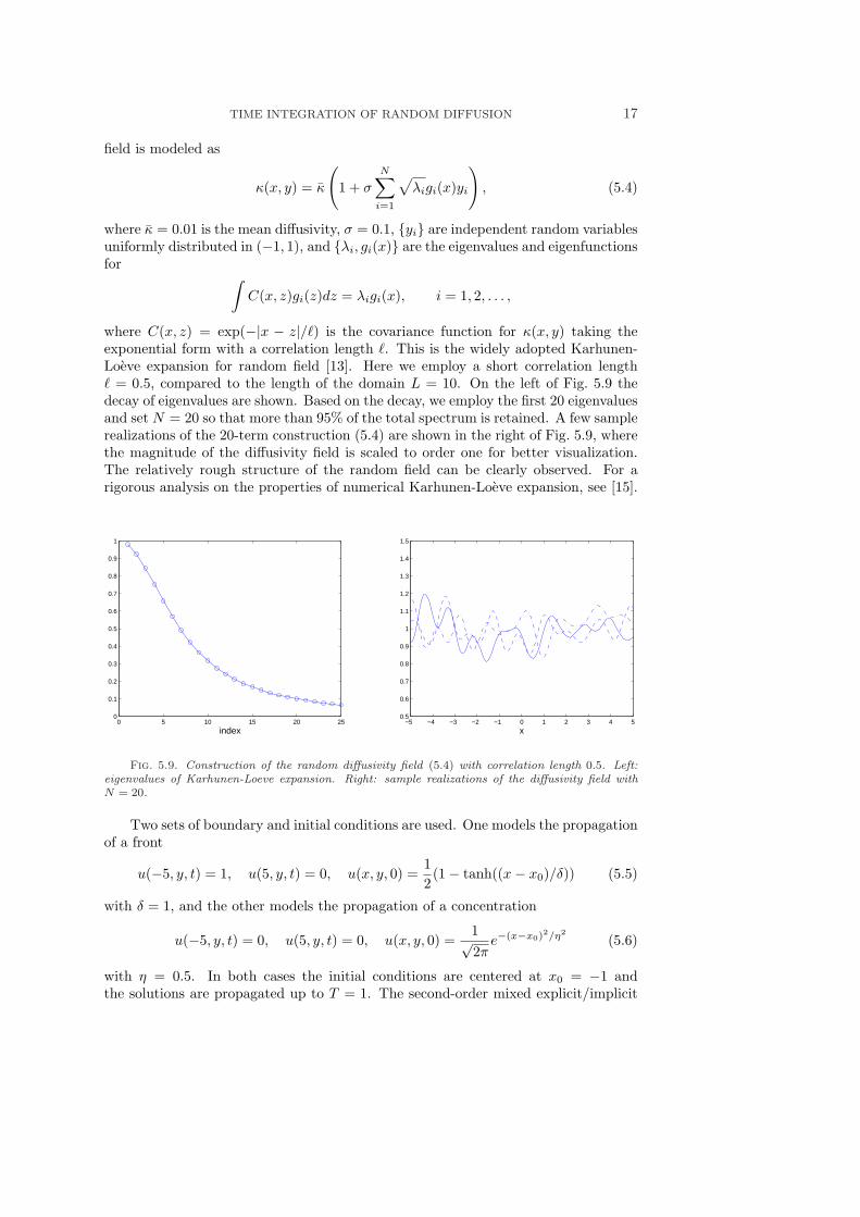
κ(x, y) = κ

(1 + σ

N∑

i=1

√λigi(x)yi

), (5.4)

where κ = 0.01 is the mean diffusivity, σ = 0.1, yi are independent random variablesuniformly distributed in (−1, 1), and λi, gi(x) are the eigenvalues and eigenfunctionsfor

∫C(x, z)gi(z)dz = λigi(x), i = 1, 2, . . . ,

where C(x, z) = exp(−|x − z|/`) is the covariance function for κ(x, y) taking theexponential form with a correlation length `. This is the widely adopted Karhunen-Loeve expansion for random field [13]. Here we employ a short correlation length` = 0.5, compared to the length of the domain L = 10. On the left of Fig. 5.9 thedecay of eigenvalues are shown. Based on the decay, we employ the first 20 eigenvaluesand set N = 20 so that more than 95% of the total spectrum is retained. A few samplerealizations of the 20-term construction (5.4) are shown in the right of Fig. 5.9, wherethe magnitude of the diffusivity field is scaled to order one for better visualization.The relatively rough structure of the random field can be clearly observed. For arigorous analysis on the properties of numerical Karhunen-Loeve expansion, see [15].

0 5 10 15 20 250

0.1

0.2

0.3

0.4

0.5

0.6

0.7

0.8

0.9

1

index−5 −4 −3 −2 −1 0 1 2 3 4 5

0.5

0.6

0.7

0.8

0.9

1

1.1

1.2

1.3

1.4

1.5

x

Fig. 5.9. Construction of the random diffusivity field (5.4) with correlation length 0.5. Left:eigenvalues of Karhunen-Loeve expansion. Right: sample realizations of the diffusivity field withN = 20.

Two sets of boundary and initial conditions are used. One models the propagationof a front

u(−5, y, t) = 1, u(5, y, t) = 0, u(x, y, 0) =12(1− tanh((x− x0)/δ)) (5.5)

with δ = 1, and the other models the propagation of a concentration

u(−5, y, t) = 0, u(5, y, t) = 0, u(x, y, 0) =1√2π

e−(x−x0)2/η2

(5.6)

with η = 0.5. In both cases the initial conditions are centered at x0 = −1 andthe solutions are propagated up to T = 1. The second-order mixed explicit/implicit


scheme (4.16) is employed with ∆t = 0.005. The spatial discretization is the modal-type spectral/hp element method ([10]) with 10 elements, each one of 12th order.

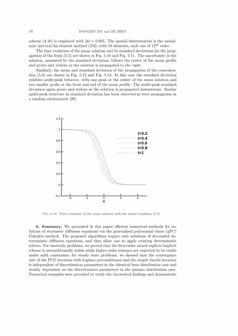
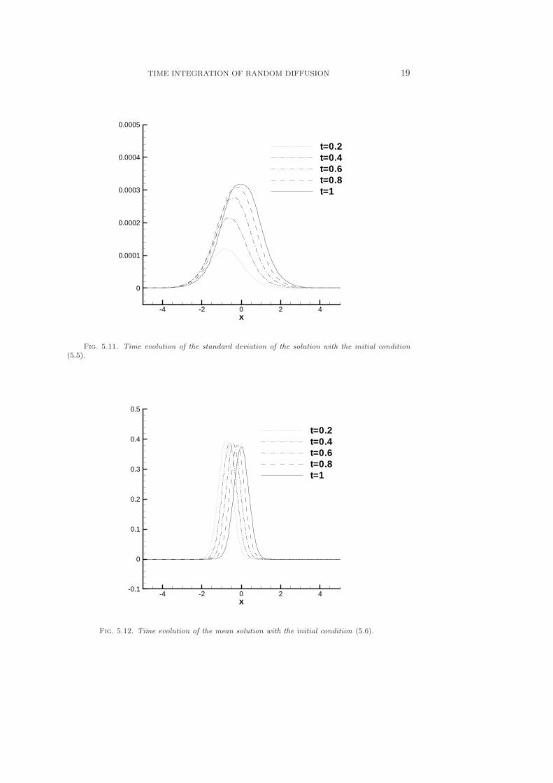
The time evolution of the mean solution and its standard deviations for the prop-agation of the front (5.5) are shown in Fig. 5.10 and Fig. 5.11. The uncertainty in thesolution, measured by the standard deviation, follows the center of the mean profileand grows and widens as the solution is propagated to the right.

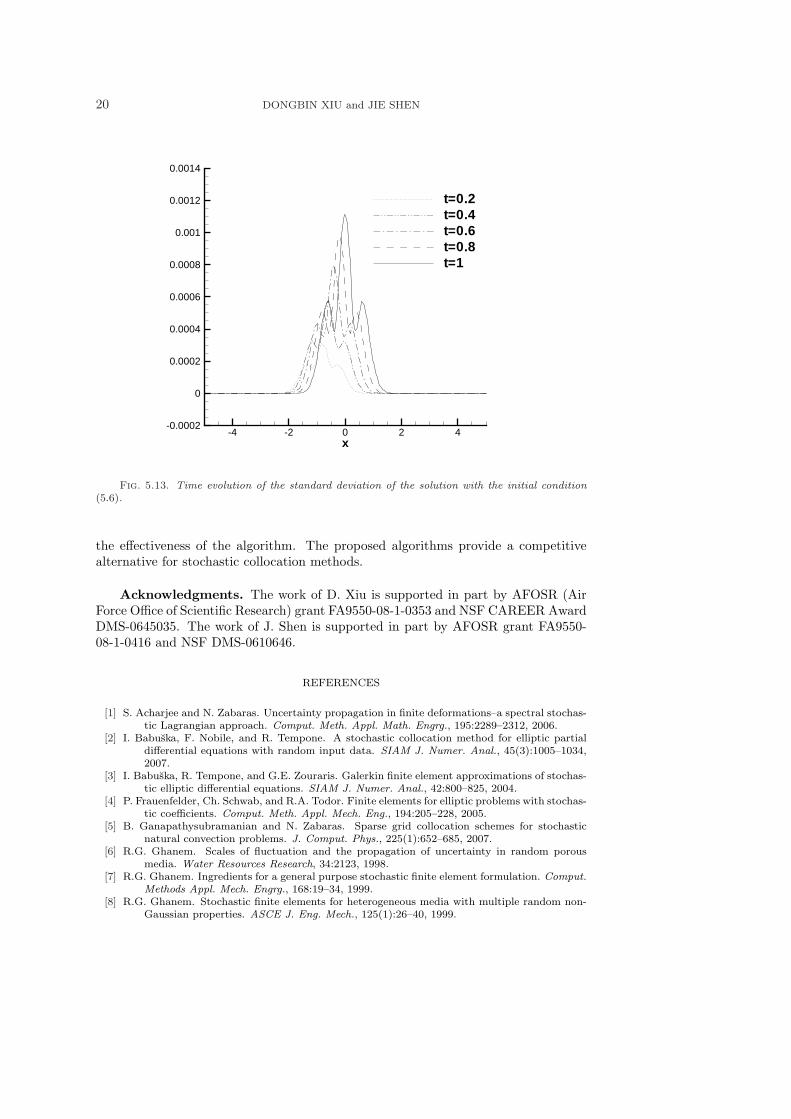
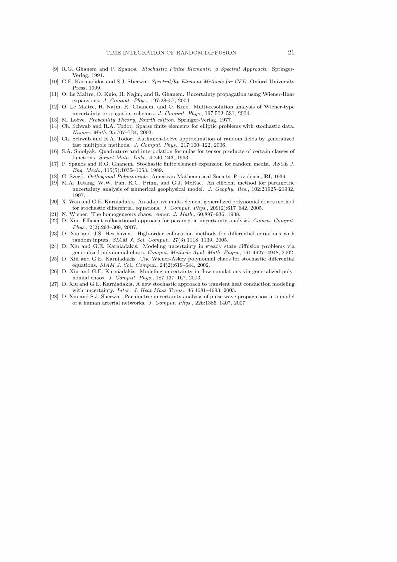
Similarly, the mean and standard deviation of the propagation of the concentra-tion (5.6) are shown in Fig. 5.12 and Fig. 5.13. In this case the standard deviationexhibits multi-peak behavior, with one peak at the center of the mean solution andtwo smaller peaks at the front and end of the mean profile. The multi-peak standarddeviation again grows and widens as the solution is propagated downstream. Similarmulti-peak structure in standard deviation has been observed in wave propagation ina random environment [28].

x-4 -2 0 2 4

-0.2

0

0.2

0.4

0.6

0.8

1

1.2

t=0.2t=0.4t=0.6t=0.8t=1

Fig. 5.10. Time evolution of the mean solution with the initial condition (5.5).

6. Summary. We presented in this paper efficient numerical methods for so-lutions of stochastic diffusion equations via the generalized polynomial chaos (gPC)Galerkin method. The proposed algorithms require only solutions of decoupled de-terministic diffusion equations, and thus allow one to apply existing deterministicsolvers. For unsteady problems, we proved that the first-order mixed explicit/implicitscheme is unconditionally stable while higher-order schemes are expected to be stableunder mild constraints; for steady state problems, we showed that the convergencerate of the PCG iteration with Laplace preconditioner and the simple Jacobi iterationis independent of discretization parameters in the identical beta distribution case andweakly dependent on the discretization parameters in the gamma distribution case.Numerical examples were provided to verify the theoretical findings and demonstrate


x-4 -2 0 2 4

0

0.0001

0.0002

0.0003

0.0004

0.0005

t=0.2t=0.4t=0.6t=0.8t=1

Fig. 5.11. Time evolution of the standard deviation of the solution with the initial condition(5.5).

x-4 -2 0 2 4

-0.1

0

0.1

0.2

0.3

0.4

0.5

t=0.2t=0.4t=0.6t=0.8t=1

Fig. 5.12. Time evolution of the mean solution with the initial condition (5.6).


x-4 -2 0 2 4

-0.0002

0

0.0002

0.0004

0.0006

0.0008

0.001

0.0012

0.0014

t=0.2t=0.4t=0.6t=0.8t=1

Fig. 5.13. Time evolution of the standard deviation of the solution with the initial condition(5.6).

the effectiveness of the algorithm. The proposed algorithms provide a competitivealternative for stochastic collocation methods.

Acknowledgments. The work of D. Xiu is supported in part by AFOSR (AirForce Office of Scientific Research) grant FA9550-08-1-0353 and NSF CAREER AwardDMS-0645035. The work of J. Shen is supported in part by AFOSR grant FA9550-08-1-0416 and NSF DMS-0610646.

REFERENCES

[1] S. Acharjee and N. Zabaras. Uncertainty propagation in finite deformations–a spectral stochas-tic Lagrangian approach. Comput. Meth. Appl. Math. Engrg., 195:2289–2312, 2006.

[2] I. Babuska, F. Nobile, and R. Tempone. A stochastic collocation method for elliptic partialdifferential equations with random input data. SIAM J. Numer. Anal., 45(3):1005–1034,2007.

[3] I. Babuska, R. Tempone, and G.E. Zouraris. Galerkin finite element approximations of stochas-tic elliptic differential equations. SIAM J. Numer. Anal., 42:800–825, 2004.

[4] P. Frauenfelder, Ch. Schwab, and R.A. Todor. Finite elements for elliptic problems with stochas-tic coefficients. Comput. Meth. Appl. Mech. Eng., 194:205–228, 2005.

[5] B. Ganapathysubramanian and N. Zabaras. Sparse grid collocation schemes for stochasticnatural convection problems. J. Comput. Phys., 225(1):652–685, 2007.

[6] R.G. Ghanem. Scales of fluctuation and the propagation of uncertainty in random porousmedia. Water Resources Research, 34:2123, 1998.

[7] R.G. Ghanem. Ingredients for a general purpose stochastic finite element formulation. Comput.Methods Appl. Mech. Engrg., 168:19–34, 1999.

[8] R.G. Ghanem. Stochastic finite elements for heterogeneous media with multiple random non-Gaussian properties. ASCE J. Eng. Mech., 125(1):26–40, 1999.


[9] R.G. Ghanem and P. Spanos. Stochastic Finite Elements: a Spectral Approach. Springer-Verlag, 1991.

[10] G.E. Karniadakis and S.J. Sherwin. Spectral/hp Element Methods for CFD. Oxford UniversityPress, 1999.

[11] O. Le Maitre, O. Knio, H. Najm, and R. Ghanem. Uncertainty propagation using Wiener-Haarexpansions. J. Comput. Phys., 197:28–57, 2004.

[12] O. Le Maitre, H. Najm, R. Ghanem, and O. Knio. Multi-resolution analysis of Wiener-typeuncertainty propagation schemes. J. Comput. Phys., 197:502–531, 2004.

[13] M. Loeve. Probability Theory, Fourth edition. Springer-Verlag, 1977.[14] Ch. Schwab and R.A. Todor. Sparse finite elements for elliptic problems with stochastic data.

Numer. Math, 95:707–734, 2003.[15] Ch. Schwab and R.A. Todor. Karhunen-Loeve approximation of random fields by generalized

fast multipole methods. J. Comput. Phys., 217:100–122, 2006.[16] S.A. Smolyak. Quadrature and interpolation formulas for tensor products of certain classes of

functions. Soviet Math. Dokl., 4:240–243, 1963.[17] P. Spanos and R.G. Ghanem. Stochastic finite element expansion for random media. ASCE J.

Eng. Mech., 115(5):1035–1053, 1989.[18] G. Szego. Orthogonal Polynomials. American Mathematical Society, Providence, RI, 1939.[19] M.A. Tatang, W.W. Pan, R.G. Prinn, and G.J. McRae. An efficient method for parametric

uncertainty analysis of numerical geophysical model. J. Geophy. Res., 102:21925–21932,1997.

[20] X. Wan and G.E. Karniadakis. An adaptive multi-element generalized polynomial chaos methodfor stochastic differential equations. J. Comput. Phys., 209(2):617–642, 2005.

[21] N. Wiener. The homogeneous chaos. Amer. J. Math., 60:897–936, 1938.[22] D. Xiu. Efficient collocational approach for parametric uncertainty analysis. Comm. Comput.

Phys., 2(2):293–309, 2007.[23] D. Xiu and J.S. Hesthaven. High-order collocation methods for differential equations with

random inputs. SIAM J. Sci. Comput., 27(3):1118–1139, 2005.[24] D. Xiu and G.E. Karniadakis. Modeling uncertainty in steady state diffusion problems via

generalized polynomial chaos. Comput. Methods Appl. Math. Engrg., 191:4927–4948, 2002.[25] D. Xiu and G.E. Karniadakis. The Wiener-Askey polynomial chaos for stochastic differential

equations. SIAM J. Sci. Comput., 24(2):619–644, 2002.[26] D. Xiu and G.E. Karniadakis. Modeling uncertainty in flow simulations via generalized poly-

nomial chaos. J. Comput. Phys., 187:137–167, 2003.[27] D. Xiu and G.E. Karniadakis. A new stochastic approach to transient heat conduction modeling

with uncertainty. Inter. J. Heat Mass Trans., 46:4681–4693, 2003.[28] D. Xiu and S.J. Sherwin. Parametric uncertainty analysis of pulse wave propagation in a model

of a human arterial networks. J. Comput. Phys., 226:1385–1407, 2007.

efficient stochastic galerkin methods for random …shen/pub/xiu_jcp08.pdf · efficient stochastic...

Documents