random variables and stochastic processes -...
TRANSCRIPT
1
Random Variables
and Stochastic Processes

2
Randomness
• The word random effectively means
unpredictable
• In engineering practice we may treat some
signals as random to simplify the analysis
even though they may not actually be
random

3
Random Variable Defined
X( )A random variable is the assignment of numerical
values to the outcomes of experiments

4
Random VariablesExamples of assignments of numbers to the outcomes of
experiments.
5
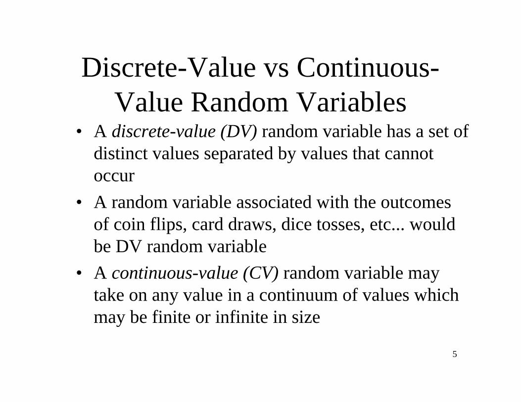
Discrete-Value vs Continuous-
Value Random Variables• A discrete-value (DV) random variable has a set of
distinct values separated by values that cannot
occur
• A random variable associated with the outcomes
of coin flips, card draws, dice tosses, etc... would
be DV random variable
• A continuous-value (CV) random variable may
take on any value in a continuum of values which
may be finite or infinite in size

6
Distribution Functions
F
Xx( ) = P X x( )
The distribution function of a random variable X is the
probability that it is less than or equal to some value,
as a function of that value.
Since the distribution function is a probability it must satisfy
the requirements for a probability.
0 F
Xx( ) 1 , < x <
F
X( ) = 0 and F
X+( ) = 1
P x
1< X x
2( ) = F
Xx
2( ) F
Xx
1( )
is a monotonic function and its derivative is never negative. F
Xx( )
7
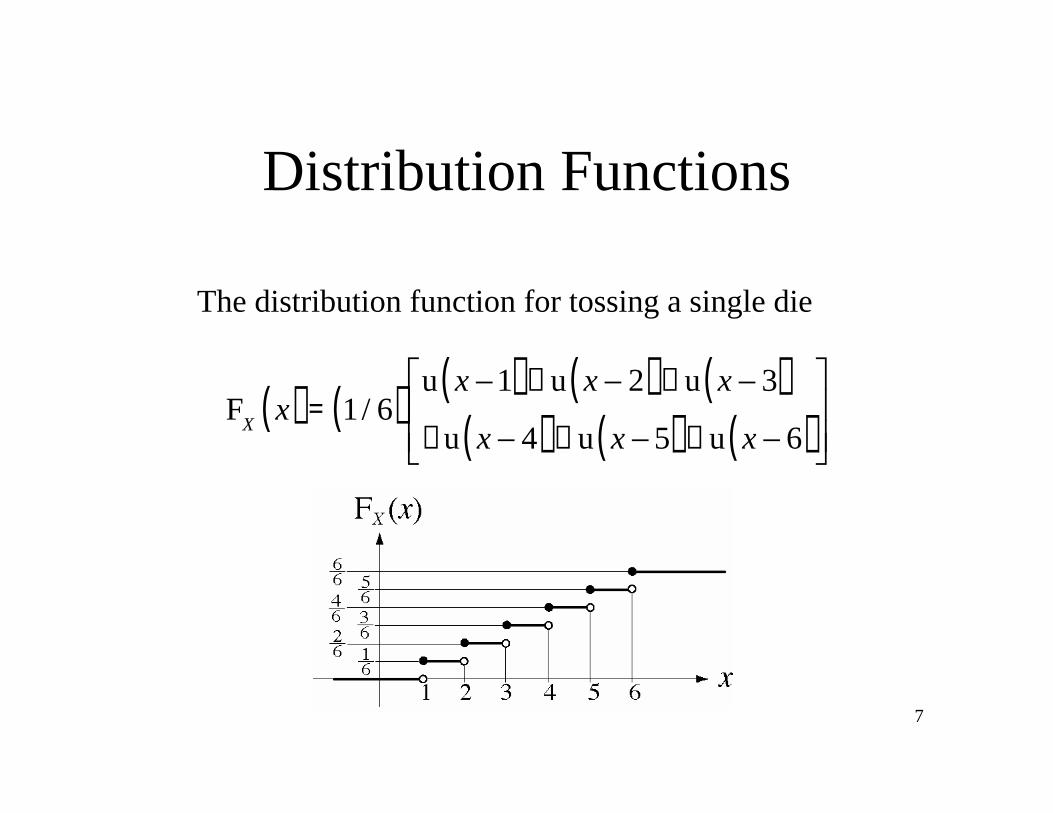
Distribution Functions
The distribution function for tossing a single die
FX
x( ) = 1/ 6( )u x 1( ) + u x 2( ) + u x 3( )+ u x 4( ) + u x 5( ) + u x 6( )

8
Distribution Functions
A possible distribution function for a continuous random
variable
9
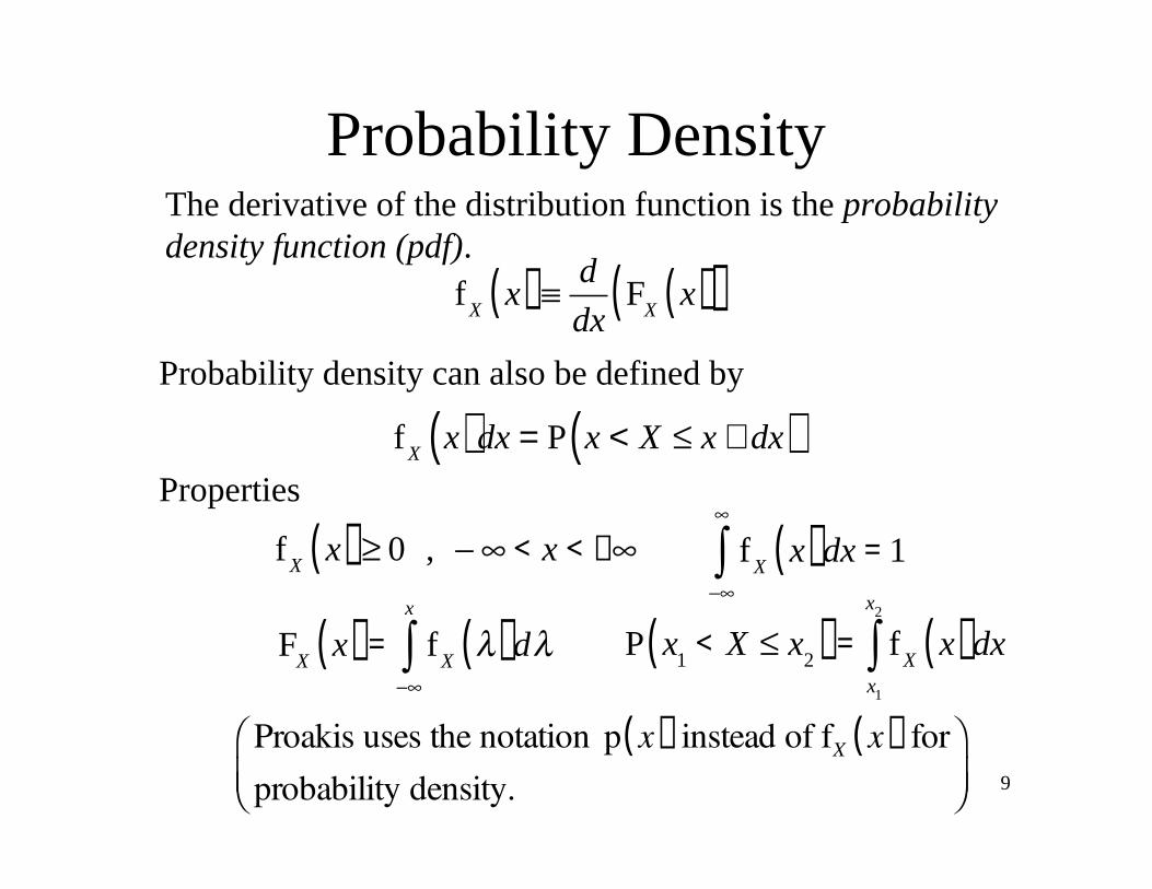
Probability DensityThe derivative of the distribution function is the probability
density function (pdf).
f
Xx( )
d
dxF
Xx( )( )
Probability density can also be defined by
f
Xx( )dx = P x < X x + dx( )
Properties
f
Xx( ) 0 , < x < +
fX
x( )dx = 1
FX
x( ) = fX
( )d
x
P x1< X x
2( ) = f
Xx( )dx
x1
x2
Proakis uses the notation p x( ) instead of fX x( ) for
probability density.
10
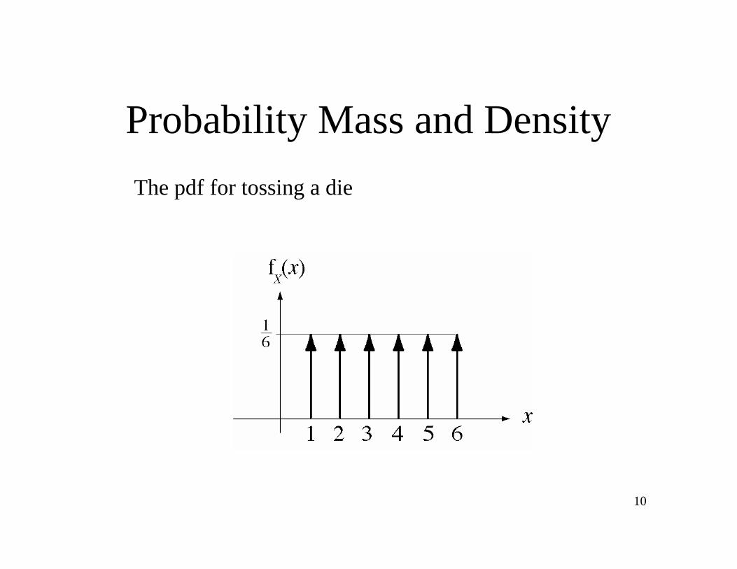
The pdf for tossing a die
Probability Mass and Density

11
Expectation and Moments
Imagine an experiment with M possible distinct outcomes
performed N times. The average of those N outcomes is
X =1
Nn
ix
i
i=1
M
where is the ith distinct value of X and is the number of
times that value occurred. Then
xi n
i
X =1
Nn
ix
i
i=1
M
=n
i
Nx
i
i=1
M
= rix
i
i=1
M
The expected value of X is
E X( ) = limN
ni
Nx
i
i=1
M
= limN
rix
i
i=1
M
= P X = xi
( )xi
i=1
M

12
Expectation and MomentsThe probability that X lies within some small range can be
approximated by
and the expected value is then approximated by
P xi
x
2< X x
i+
x
2f
Xx
i( ) x
E X( ) = P xi
x
2< X x
i+
x
2x
i
i=1
M
xif
Xx
i( ) x
i=1
M
where M is now the number of
subdivisions of width x
of the range of the random
variable.

13
Expectation and Moments
In the limit as x approaches zero,
E X( ) = x fX
x( )dx
Similarly
E g X( )( ) = g x( )fX
x( )dx
The nth moment of a random variable is
E Xn( ) = x
nf
Xx( )dx
14
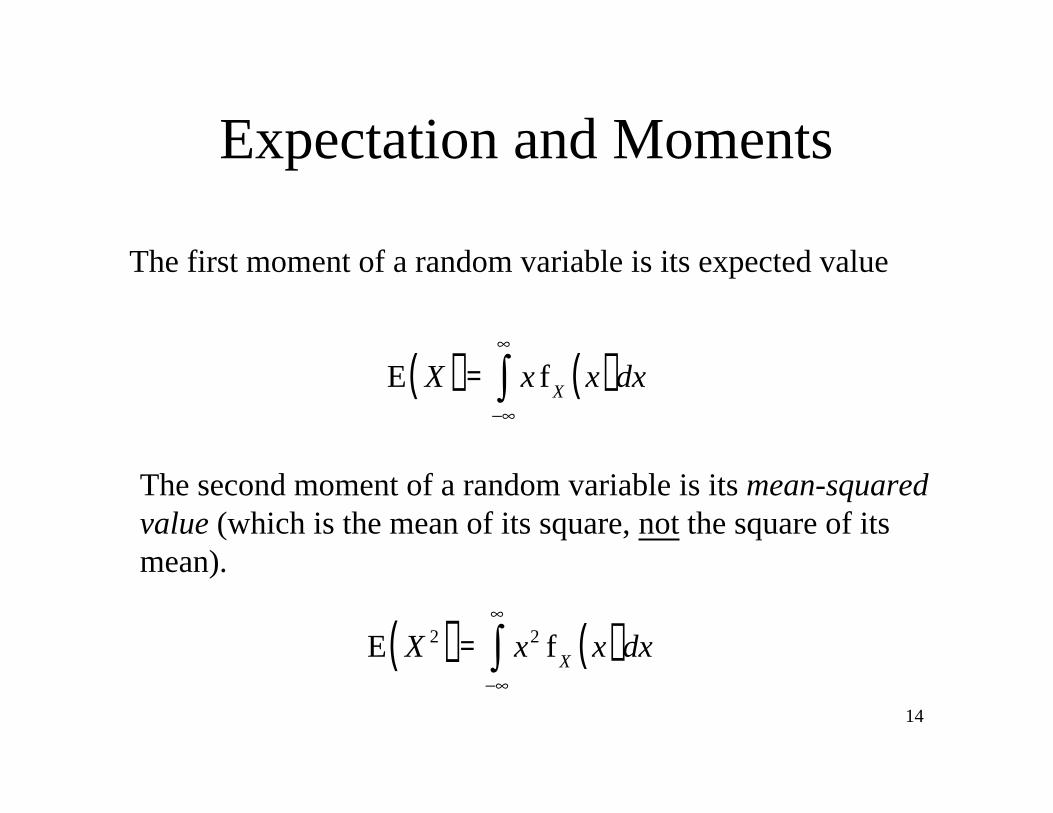
Expectation and Moments
The first moment of a random variable is its expected value
E X( ) = x fX
x( )dx
The second moment of a random variable is its mean-squared
value (which is the mean of its square, not the square of its
mean).
E X2( ) = x
2f
Xx( )dx

15
Expectation and Moments
A central moment of a random variable is the moment of
that random variable after its expected value is subtracted.
E X E X( )n
= x E X( )n
fX
x( )dx
The first central moment is always zero. The second central
moment (for real-valued random variables) is the variance,
X
2= E X E X( )
2
= x E X( )2
fX
x( )dx
The positive square root of the variance is the standard
deviation.

16
Expectation and Moments
Properties of expectation
E a( ) = a , E aX( ) = a E X( ) , E Xn
n
= E Xn
( )n
where a is a constant. These properties can be use to prove
the handy relationship,
X
2= E X
2( ) E2
X( )
The variance of a random variable is the mean of its square
minus the square of its mean.

17
Expectation and Moments
For complex-valued random variables absolute moments are useful.
The nth absolute moment of a random variable is defined by
E Xn( ) = x
n
fX
x( )dx
and the nth absolute central moment is defined by
E X E X( )n
= x E X( )n
fX
x( )dx

18
Joint Probability Density
Let X and Y be two random variables. Their joint distribution
function is
F
XYx, y( ) P X x Y y( )
0 F
XYx, y( ) 1 , < x < , < y <
F
XY,( ) = F
XYx,( ) = F
XY, y( ) = 0
F
XY,( ) = 1
F
XY, y( ) = F
Yy( ) and F
XYx,( ) = F
Xx( )
F
XYx, y( ) does not decrease if either x or y increases or both increase

19
Joint Probability DensityJoint distribution function for tossing two dice
20
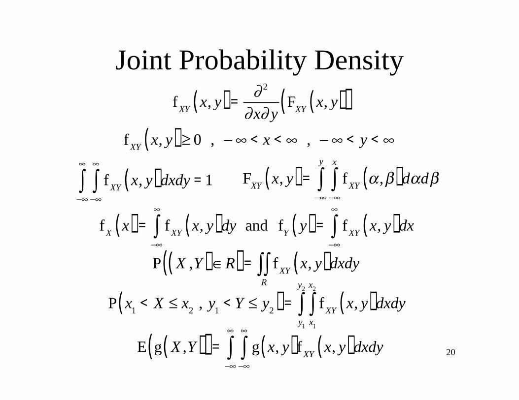
Joint Probability Density
f
XYx, y( ) =
2
x yF
XYx, y( )( )
f
XYx, y( ) 0 , < x < , < y <
fXY
x, y( )dxdy = 1
FXY
x, y( ) = fXY
,( )d
x
d
y
fX
x( ) = fXY
x, y( )dy and fY
y( ) = fXY
x, y( )dx
P x1< X x
2, y
1< Y y
2( ) = fXY
x, y( )dxx
1
x2
dyy
1
y2
E g X ,Y( )( ) = g x, y( )fXY
x, y( )dxdy
P X ,Y( ) R( ) = fXY
x, y( )dxdyR
21
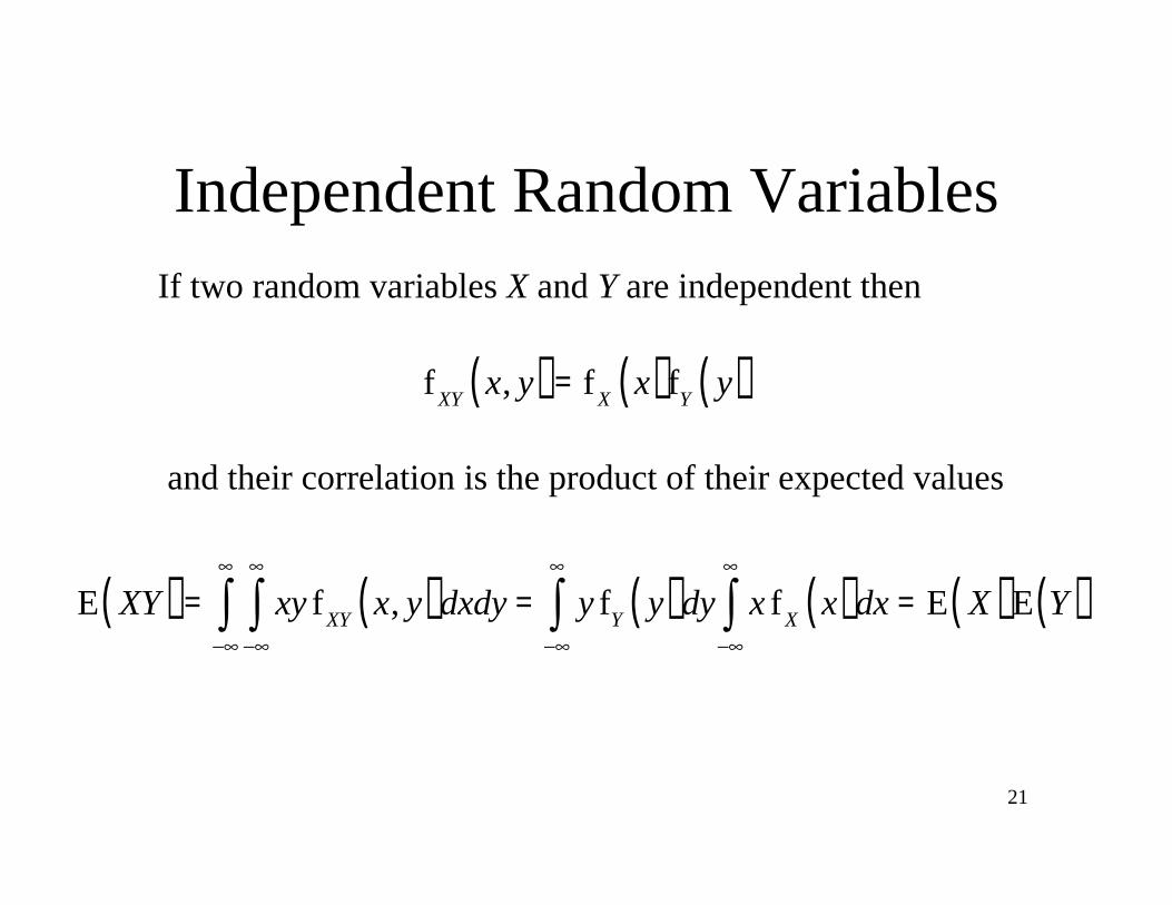
Independent Random Variables
If two random variables X and Y are independent then
f
XYx, y( ) = f
Xx( )f
Yy( )
E XY( ) = xy fXY
x, y( )dxdy = y fY
y( )dy x fX
x( )dx = E X( )E Y( )
and their correlation is the product of their expected values

22
Covariance
XYE X E X( ) Y E Y( )
*
= x E X( )( ) y*E Y *( )( )f
XYx, y( )dxdy
XY= E XY
*( ) E X( )E Y*( )
If X and Y are independent,
XY= E X( )E Y
*( ) E X( )E Y*( ) = 0
Independent Random Variables
23
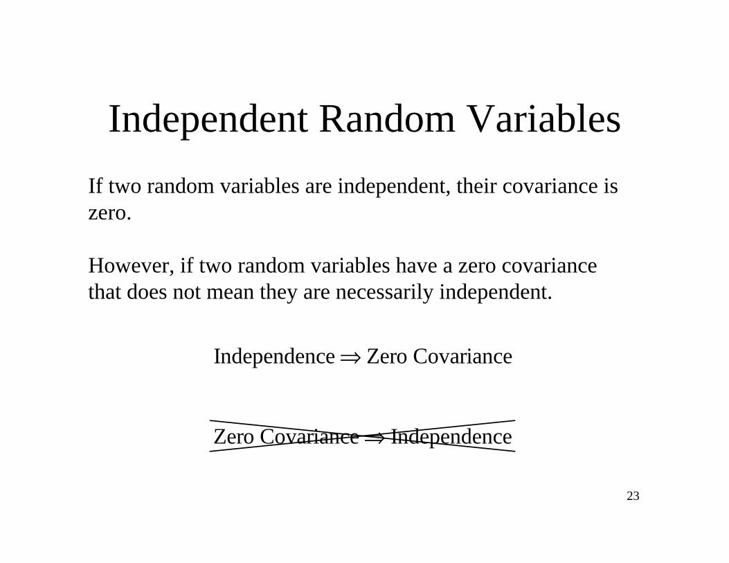
If two random variables are independent, their covariance is
zero.
However, if two random variables have a zero covariance
that does not mean they are necessarily independent.
Zero Covariance Independence
Independence Zero Covariance
Independent Random Variables
24
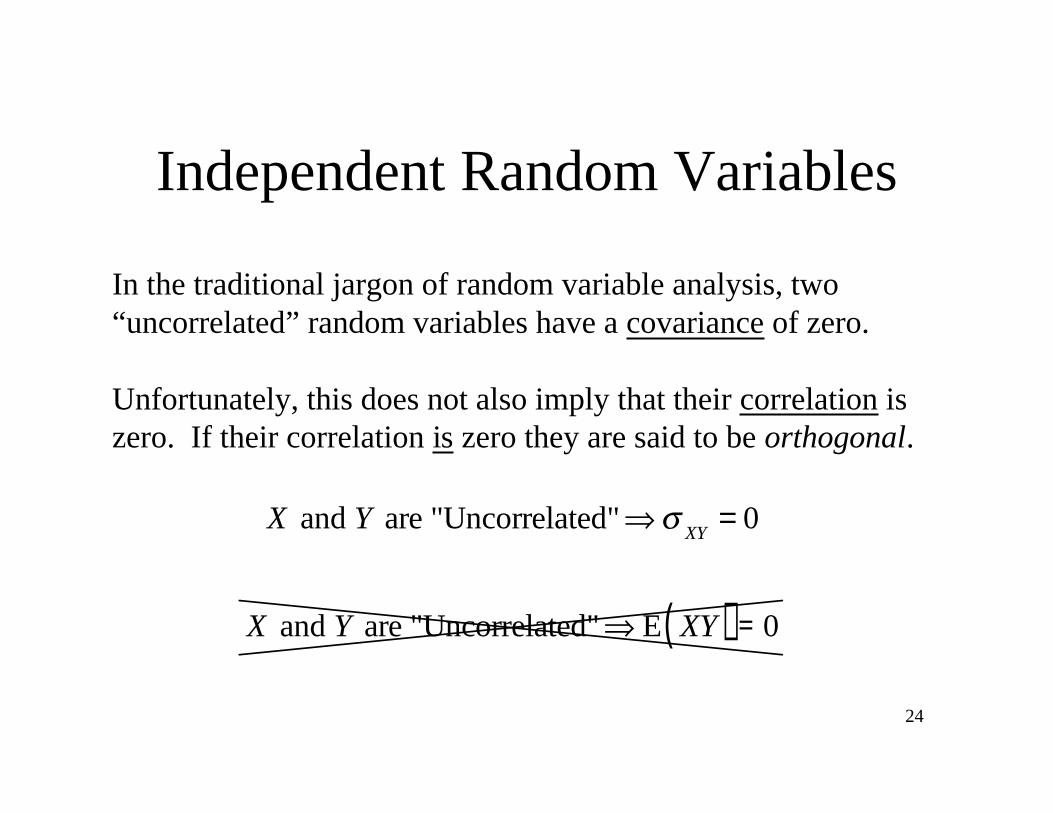
In the traditional jargon of random variable analysis, two
“uncorrelated” random variables have a covariance of zero.
Unfortunately, this does not also imply that their correlation is
zero. If their correlation is zero they are said to be orthogonal.
X and Y are "Uncorrelated"
XY= 0
X and Y are "Uncorrelated" E XY( ) = 0
Independent Random Variables
25
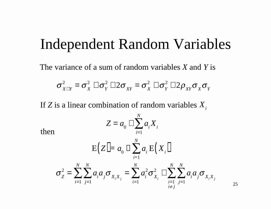
The variance of a sum of random variables X and Y is
X +Y
2=
X
2+
Y
2+ 2
XY=
X
2+
Y
2+ 2
XY X Y
If Z is a linear combination of random variables
Z = a0
+ aiX
i
i=1
N
then
E Z( ) = a0
+ aiE X
i( )
i=1
N
Z
2= a
ia
j XiX
jj=1
N
i=1
N
= ai
2
Xi
2
i=1
N
+ aia
j XiX
jj=1
N
i=1
i j
N
X
i
Independent Random Variables

26
If the X’s are all independent of each other, the variance of
the linear combination is a linear combination of the variances.
Z
2= a
i
2
Xi
2
i=1
N
If Z is simply the sum of the X’s, and the X’s are all independent
of each other, then the variance of the sum is the sum of the
variances.
Z
2=
Xi
2
i=1
N
Independent Random Variables
27
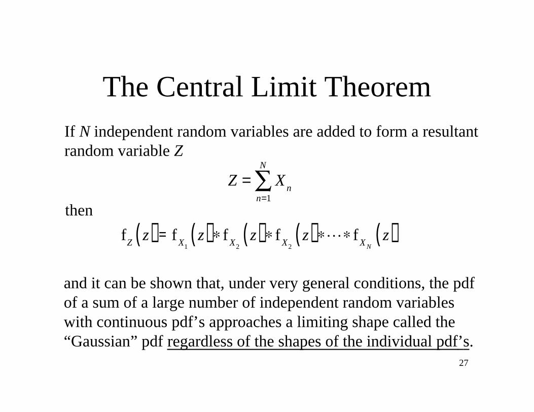
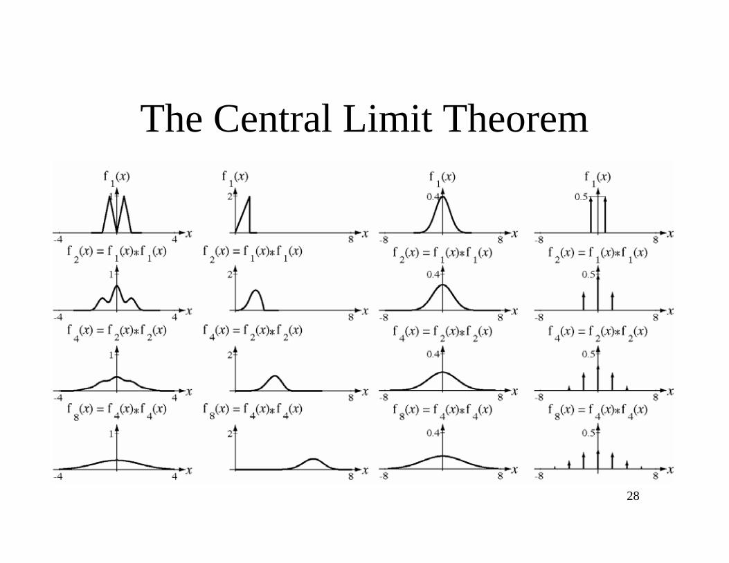
The Central Limit Theorem
If N independent random variables are added to form a resultant
random variable Z
Z = Xn
n=1
N
then
f
Zz( ) = f
X1
z( ) fX
2
z( ) fX
2
z( ) fX
N
z( )
and it can be shown that, under very general conditions, the pdf
of a sum of a large number of independent random variables
with continuous pdf’s approaches a limiting shape called the
“Gaussian” pdf regardless of the shapes of the individual pdf’s.
28
The Central Limit Theorem
29
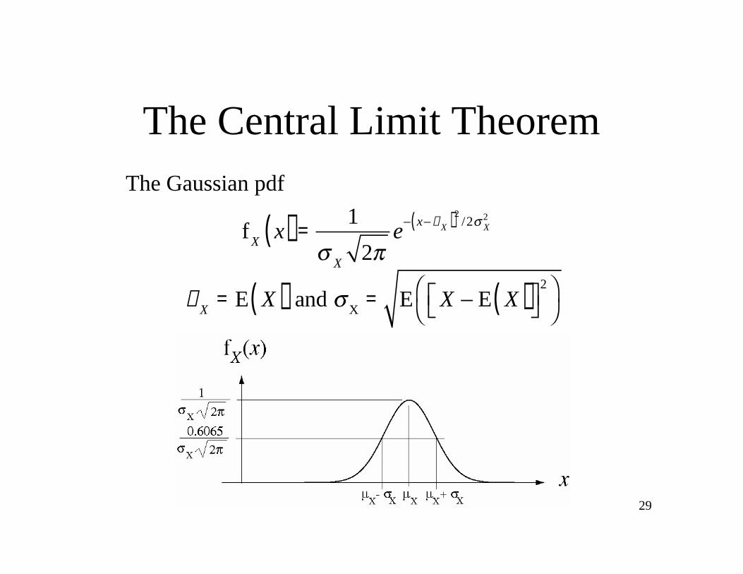
The Central Limit Theorem
The Gaussian pdf
fX
x( ) =1
X2
ex µ
X( )2
/2X
2
µX
= E X( ) and X
= E X E X( )2

30
The Central Limit TheoremThe Gaussian pdf
Its maximum value occurs at the mean value of its
argument
It is symmetrical about the mean value
The points of maximum absolute slope occur at one
standard deviation above and below the mean
Its maximum value is inversely proportional to its
standard deviation
The limit as the standard deviation approaches zero is a
unit impulse
x µx
( ) = limX
0
1
X2
ex µ
X( )2
/2X
2

31
The Central Limit Theorem
The normal pdf is a Gaussian pdf with a mean of zero and
a variance of one.
fX
x( ) =1
2
ex
2/2
The central moments of the Gaussian pdf are
E X E X( )n
=0 , n odd
1 3 5… n 1( )X
n, n even
32
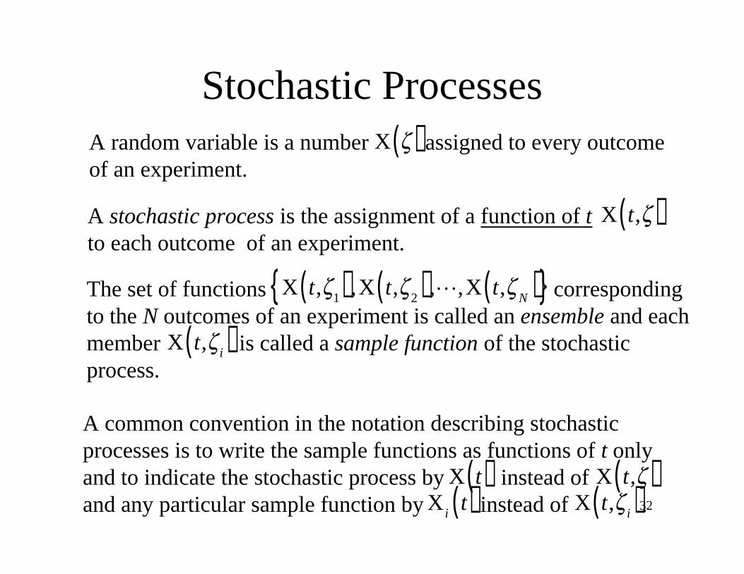
Stochastic Processes
A random variable is a number assigned to every outcome
of an experiment. X( )
A stochastic process is the assignment of a function of t
to each outcome of an experiment. X t,( )
The set of functions corresponding
to the N outcomes of an experiment is called an ensemble and each
member is called a sample function of the stochastic
process.
X t,
1( ),X t,2( ), ,X t,
N( ){ }
X t,
i( )
A common convention in the notation describing stochastic
processes is to write the sample functions as functions of t only
and to indicate the stochastic process by instead of
and any particular sample function by instead of . X t( )
X t,( )
X
it( )
X t,
i( )

33
Stochastic Processes
Ense
mble
Sample
Function
The values of at a particular time define a random variable
or just . X t( )
t1
X t
1( )
X1
34
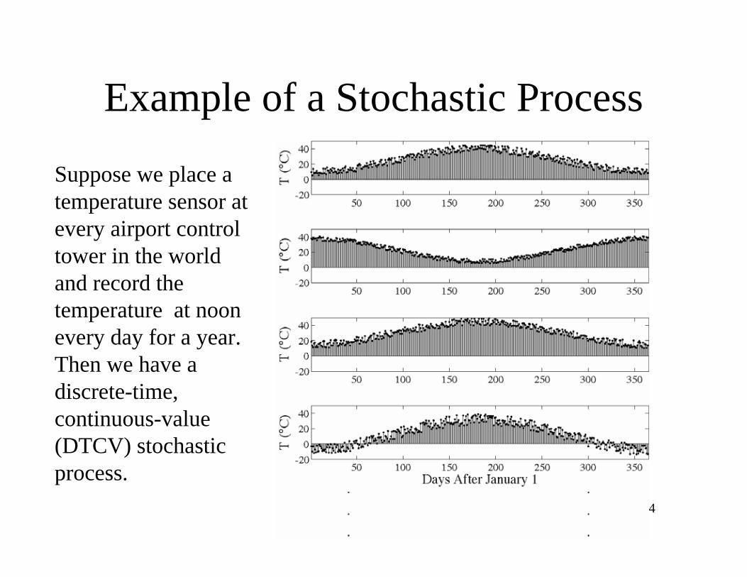
Example of a Stochastic Process
Suppose we place a
temperature sensor at
every airport control
tower in the world
and record the
temperature at noon
every day for a year.
Then we have a
discrete-time,
continuous-value
(DTCV) stochastic
process.

35
Example of a Stochastic Process
Suppose there is a large number
of people, each flipping a fair
coin every minute. If we assign
the value 1 to a head and the
value 0 to a tail we have a
discrete-time, discrete-value
(DTDV) stochastic process
36
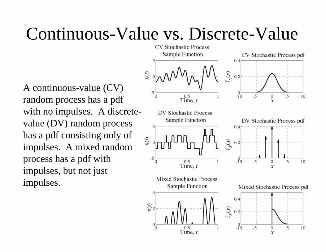
Continuous-Value vs. Discrete-Value
A continuous-value (CV)
random process has a pdf
with no impulses. A discrete-
value (DV) random process
has a pdf consisting only of
impulses. A mixed random
process has a pdf with
impulses, but not just
impulses.
37
Deterministic vs. Non-
Deterministic
A random process is deterministic if a sample function
can be described by a mathematical function such that its
future values can be computed. The randomness is in the
ensemble, not in the time functions. For example, let the
sample functions be of the form,
X t( ) = Acos 2 f
0t +( )
and let the parameter be random over the ensemble but
constant for any particular sample function.
All other random processes are non-deterministic.
38
Stationarity
If all the mltivariate statistical descriptors of a random
process are not functions of time, the random process is
said to be strict-sense stationary (SSS).
A random process is wide-sense stationary (WSS) if
E X t
1( )( )
E X t
1( )X t
2( )( )
is independent of the choice of t1
depends only on the difference between and t1
t2
and
39
Ergodicity
If all of the sample functions of a random process have the
same statistical properties the random process is said to be
ergodic. The most important consequence of ergodicity is that
ensemble moments can be replaced by time moments.
E Xn( ) = lim
T
1
TX
nt( )dt
T /2
T /2
Every ergodic random process is also stationary.
40
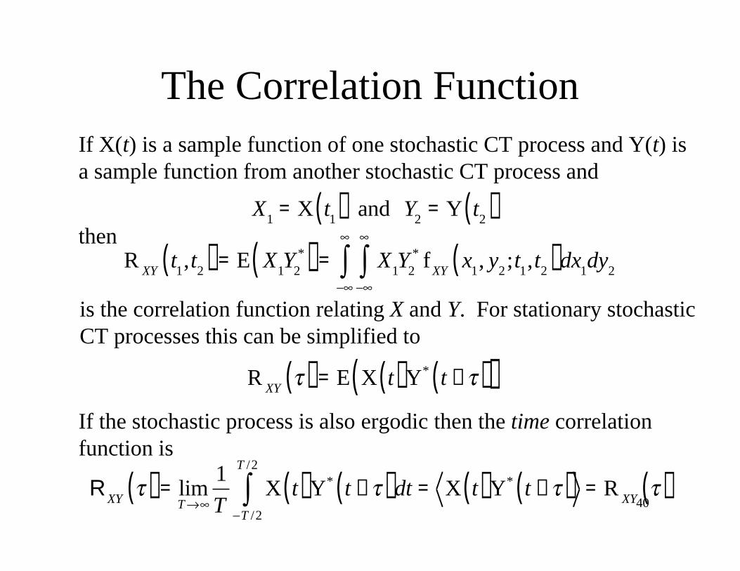
The Correlation Function
If X(t) is a sample function of one stochastic CT process and Y(t) is
a sample function from another stochastic CT process and
X
1= X t
1( ) and Y
2= Y t
2( )
then
RXY
t1,t
2( ) = E X1Y
2
*( ) = X1Y
2
*f
XYx
1, y
2;t
1,t
2( )dx1dy
2
is the correlation function relating X and Y. For stationary stochastic
CT processes this can be simplified to
R
XY( ) = E X t( )Y
*t +( )( )
If the stochastic process is also ergodic then the time correlation
function is
RXY
( ) = limT
1
TX t( )Y
*t +( )dt
T /2
T /2
= X t( )Y*
t +( ) = RXY
( )
41
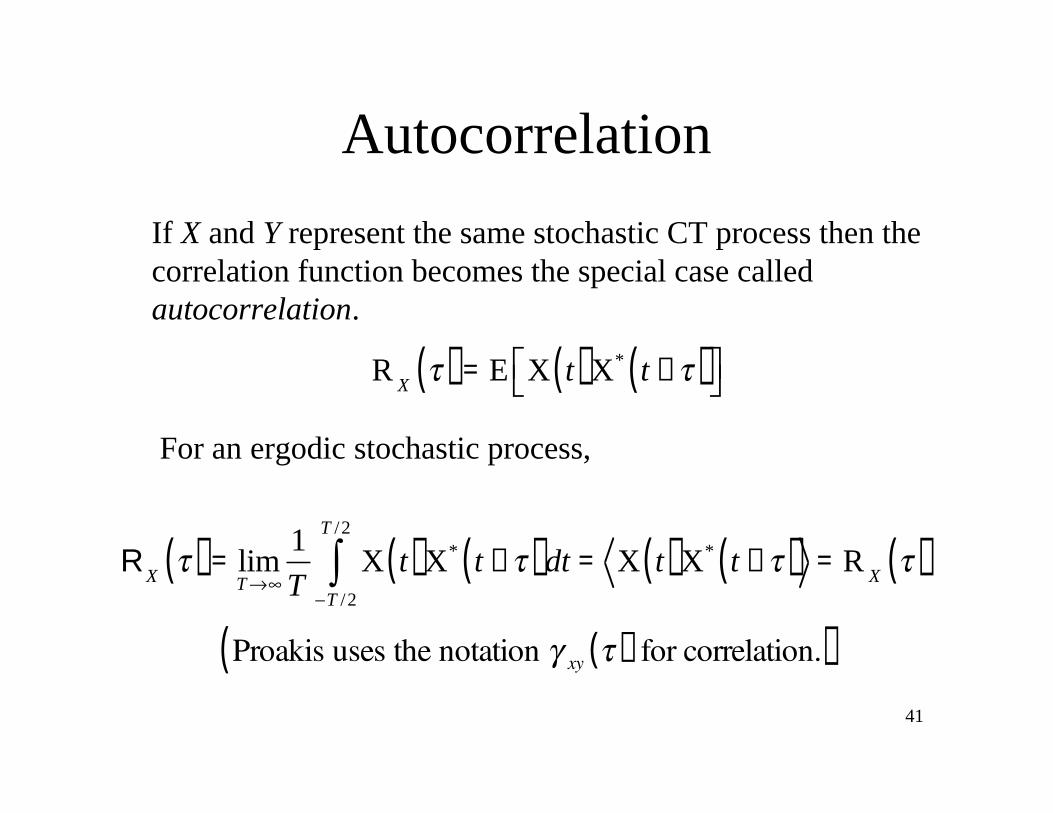
Autocorrelation
If X and Y represent the same stochastic CT process then the
correlation function becomes the special case called
autocorrelation.
R
X( ) = E X t( )X
*t +( )
For an ergodic stochastic process,
RX
( ) = limT
1
TX t( )X
*t +( )dt
T /2
T /2
= X t( )X*
t +( ) = RX
( )
Proakis uses the notation xy ( ) for correlation.( )
42
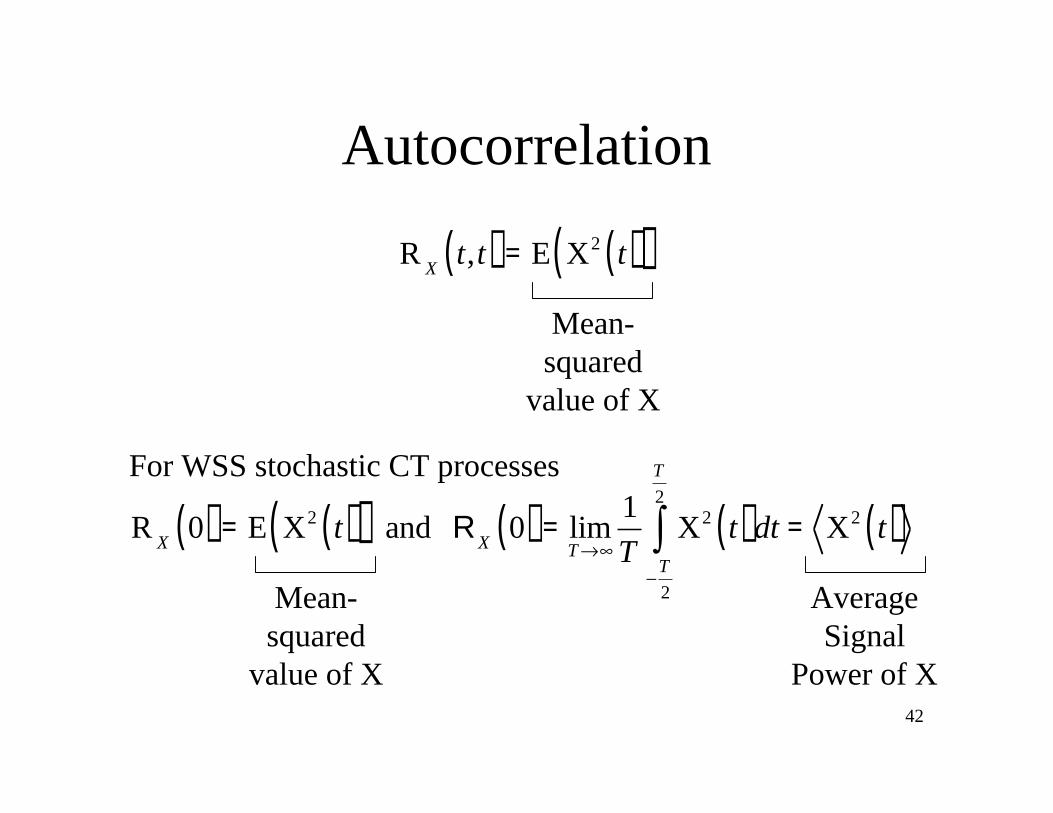
Autocorrelation
R
Xt,t( ) = E X
2t( )( )
Mean-
squared
value of X
RX
0( ) = E X2
t( )( ) and RX
0( ) = limT
1
TX
2t( )dt
T
2
T
2
= X2
t( )
Mean-
squared
value of X
Average
Signal
Power of X
For WSS stochastic CT processes

43
The Correlation Function
If is a sample function of one stochastic DT process and
is a sample function from another stochastic DT process and
X
1= X n
1and Y
2= Y n
2
then
RXY
n1,n
2= E X
1Y
2
*( ) = X1Y
2
*f
XYx
1, y
2;n
1,n
2( )dx1dy
2
is the correlation function relating X and Y. For stationary stochastic
DT processes this can be simplified to
R
XYm = E X n Y
*n + m( )
If the stochastic DT process is also ergodic then the time correlation
function is
RXY
m = limN
1
2NX n Y
*n + m
n= N
N 1
= X n Y*
n + m = RXY
m
X n
Y n
44
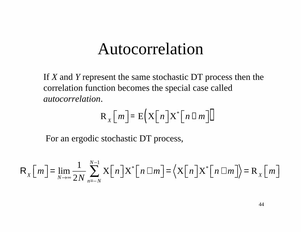
Autocorrelation
If X and Y represent the same stochastic DT process then the
correlation function becomes the special case called
autocorrelation.
R
Xm = E X n X
*n + m( )
For an ergodic stochastic DT process,
RX
m = limN
1
2NX n X
*n + m
n= N
N 1
= X n X*
n + m = RX
m
45
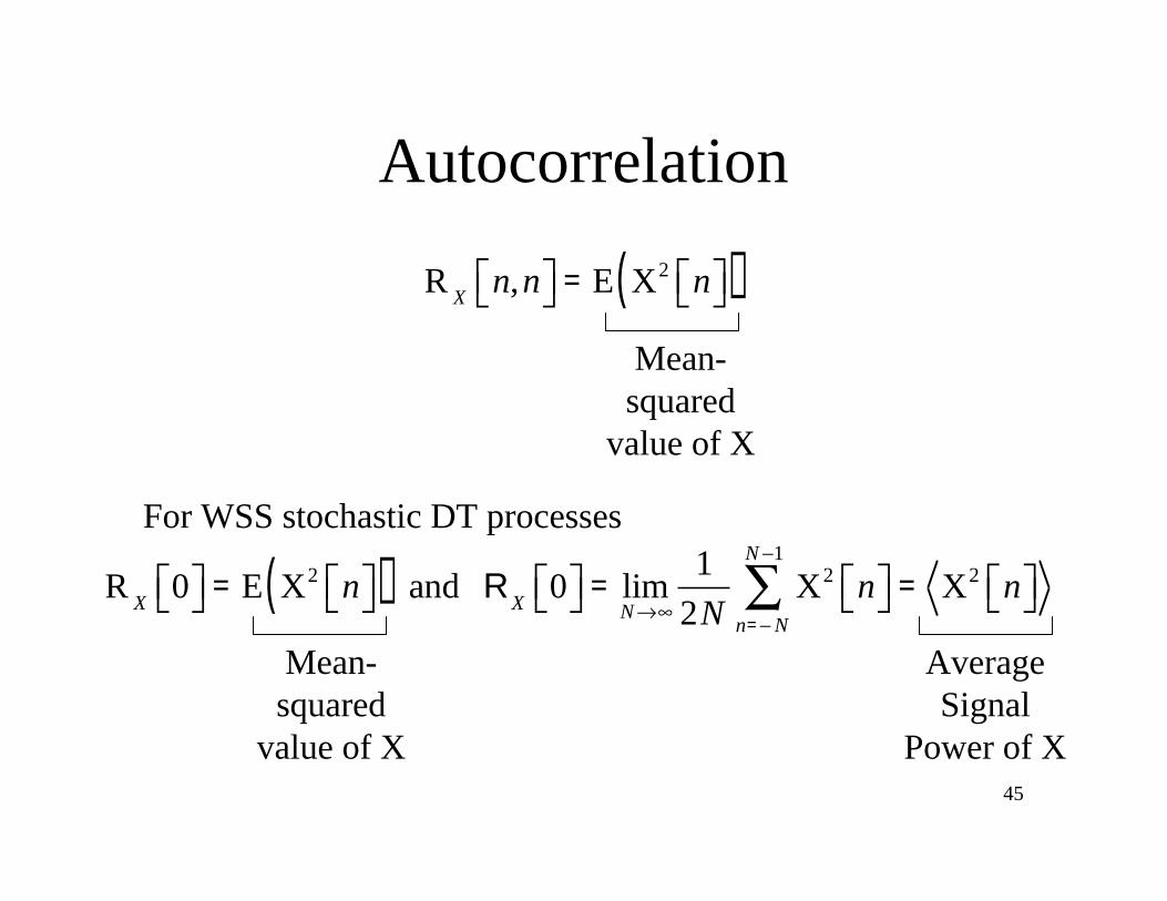
Autocorrelation
R
Xn,n = E X
2n( )
Mean-
squared
value of X
RX
0 = E X2
n( ) and RX
0 = limN
1
2NX
2n
n= N
N 1
= X2
n
Mean-
squared
value of X
Average
Signal
Power of X
For WSS stochastic DT processes
46
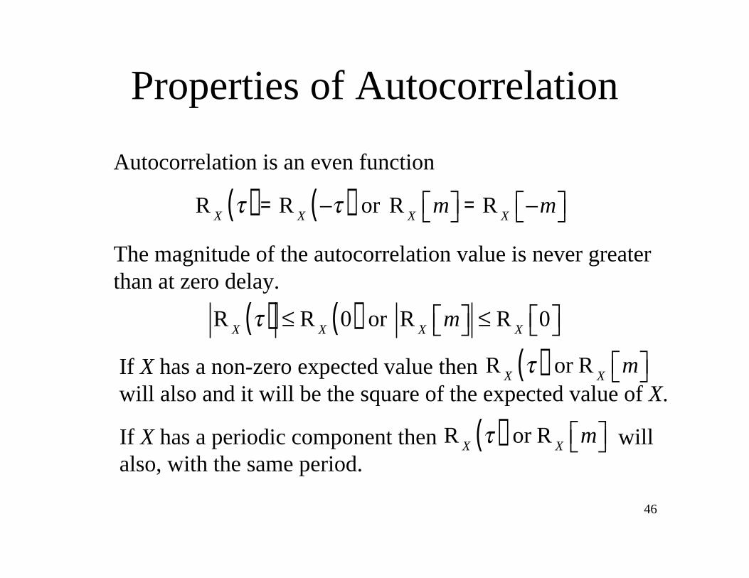
Properties of Autocorrelation
Autocorrelation is an even function
R
X( ) = R
X( ) or R
Xm = R
Xm
The magnitude of the autocorrelation value is never greater
than at zero delay.
R
X( ) R
X0( ) or R
Xm R
X0
If X has a non-zero expected value then
will also and it will be the square of the expected value of X. R
X( ) or R
Xm
If X has a periodic component then will
also, with the same period. R
X( ) or R
Xm

47
Properties of Autocorrelation
If is ergodic with zero mean and no periodic components
then
limRX
( ) = 0 or limm
RX
m = 0
X t( ){ }
Only autocorrelation functions for which
F R
X ( ){ } 0 for all f or F RX
m{ } 0 for all
are possible
A time shift of a function does not affect its autocorrelation

48
Autocovariance
C
X( ) = R
X( ) E
2X( ) or C
Xm = R
Xm E
2X( )
Autocovariance is similar to autocorrelation. Autocovariance
is the autocorrelation of the time-varying part of a signal.

49
CrosscorrelationProperties
R
XY( ) = R
YX( ) or R
XYm = R
YXm
R
XY( ) R
X0( )R
Y0( ) or R
XYm R
X0 R
Y0
If two stochastic processes X and Y are statistically independent
R
XY( ) = E X( )E Y
*( ) = RYX
( ) or RXY
m = E X( )E Y*( ) = R
YXm
If X is stationary CT and is its time derivative X
R
XX( ) =
d
dR
X( )( )
RX
( ) =d
2
d2
RX
( )( )
If and X and Y are independent and at least
one of them has a zero mean Z t( ) = X t( ) ± Y t( )
R
Z( ) = R
X( ) + R
Y( )

50
Power Spectral Density
In applying frequency-domain techniques to the analysis of
random signals the natural approach is to Fourier transform
the signals.
Unfortunately the Fourier transform of a stochastic process
does not, strictly speaking, exist because it has infinite
signal energy.
But the Fourier transform of a truncated version of a
stochastic process does exist.

51
Power Spectral Density
XT
t( ) =X t( ) , t T / 2
0 , t > T / 2= X t( )rect t / T( )
The Fourier transform is
Using Parseval’s theorem,
Dividing through by T,
F XT
t( )( ) = XT
t( )e j2 ftdt , T <
XT
t( )2
dtT /2
T /2
= F XT
t( )( )2
df
1
TX
T
2 t( )dtT /2
T /2
=1
TF X
Tt( )( )
2
df
For a CT stochastic process let
52
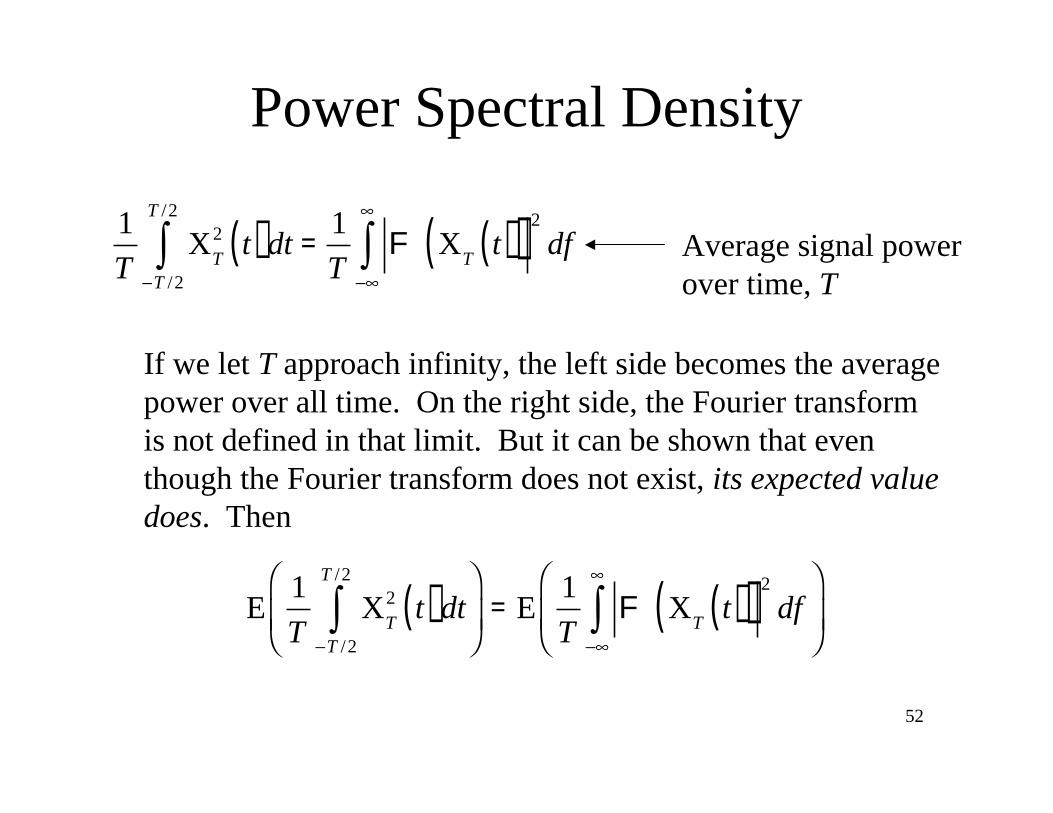
Power Spectral Density
Average signal power
over time, T
If we let T approach infinity, the left side becomes the average
power over all time. On the right side, the Fourier transform
is not defined in that limit. But it can be shown that even
though the Fourier transform does not exist, its expected value
does. Then
E1
TX
T
2 t( )dtT /2
T /2
= E1
TF X
Tt( )( )
2
df
1
TX
T
2 t( )dtT /2
T /2
=1
TF X
Tt( )( )
2
df

53
Power Spectral Density
limT
1
TE X
2( )dtT /2
T /2
= limT
1
TE F X
Tt( )( )
2
df
Taking the limit as T approaches infinity,
E X 2( ) = limT
E
F XT
t( )( )2
Tdf
The integrand on the right side is identified as power spectral
density (PSD).
GX
f( ) = limT
E
F XT
t( )( )2
T
Proakis uses the notation XX F( ) for power spectral density.( )

54
Power Spectral Density
GX
f( )df = mean squared value of X t( ){ }
GX
f( )df = average power of X t( ){ }
PSD is a description of the variation of a signal’s power versus
frequency.
PSD can be (and often is) conceived as single-sided, in which
all the power is accounted for in positive frequency space.

55
PSD Concept

56
PSD of DT Stochastic Processes
GX
F( ) = limN
E
F XT
n( )2
N
G
XF( )dF
1= mean squared value of X n{ }
1
2G
X( )d
2= mean squared value of X n{ }
x n = F
1X F( )( ) = X F( )e j2 FndF
1
FX F( ) = F x n( ) = x n e j2 Fn
n=
x n = F
1X( )( ) =
1
2X( )e j nd
2
FX( ) = F x n( ) = x n e j n
n=
where the Fourier transform is the discrete-time Fourier transform
(DTFT) defined by
or

57
PSD and Autocorrelation
It can be shown that PSD and autocorrelation form a Fourier
transform pair.
G
Xf( ) = F R
X ( )( ) or GX
F( ) = F RX
m( )
58
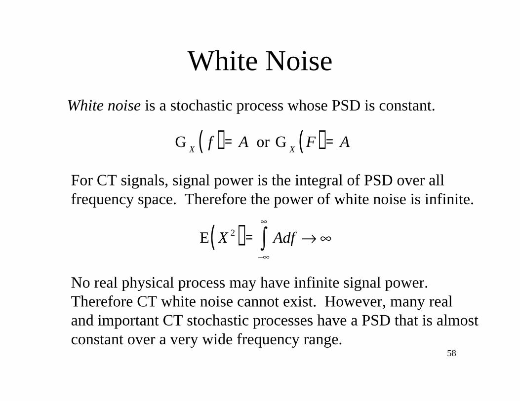
White Noise
White noise is a stochastic process whose PSD is constant.
G
Xf( ) = A or G
XF( ) = A
For CT signals, signal power is the integral of PSD over all
frequency space. Therefore the power of white noise is infinite.
E X 2( ) = Adf
No real physical process may have infinite signal power.
Therefore CT white noise cannot exist. However, many real
and important CT stochastic processes have a PSD that is almost
constant over a very wide frequency range.

59
White Noise
In many kinds of CT noise analysis, a type of random variable
known as bandlimited white noise is used. Bandlimited
white noise is simply the response of an ideal lowpass filter
which is excited by white noise.
The PSD of bandlimited white noise is constant over a finite
frequency range and zero outside that range.
Bandlimited white noise has finite signal power.

60
Cross Power Spectral Density
PSD is the Fourier transform of autocorrelation.
Cross power spectral density is the Fourier transform of
cross correlation.
Properties:
G
XYf( ) = G
YX
* f( ) or GXY
F( ) = GYX
* F( )
R
XYt( ) F
GXY
f( ) or RXY
nF
GXY
F( )
Re G
XYf( )( ) and Re G
YXf( )( ) are both even
Im G
XYf( )( ) and Im G
YXf( )( ) are both odd
61
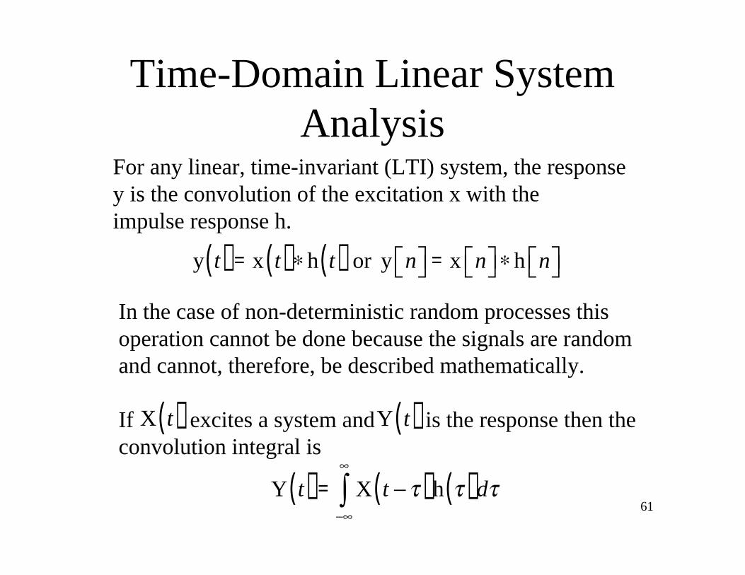
Time-Domain Linear System
AnalysisFor any linear, time-invariant (LTI) system, the response
y is the convolution of the excitation x with the
impulse response h.
y t( ) = x t( ) h t( ) or y n = x n h n
In the case of non-deterministic random processes this
operation cannot be done because the signals are random
and cannot, therefore, be described mathematically.
If excites a system and is the response then the
convolution integral is
Y t( ) = X t( )h( )d
X t( )
Y t( )
62
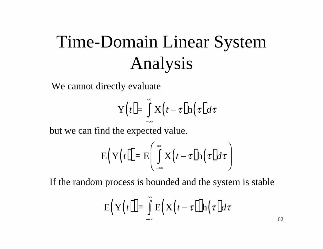
Time-Domain Linear System
Analysis
Y t( ) = X t( )h( )d
We cannot directly evaluate
but we can find the expected value.
E Y t( )( ) = E X t( )h( )d
If the random process is bounded and the system is stable
E Y t( )( ) = E X t( )( )h( )d

63
Time-Domain Linear System
AnalysisIf the random process X is stationary
E Y t( )( ) = E X t( )( )h( )d E Y( ) = E X( ) h( )d
Using
h t( )dt = H 0( ) E Y( ) = E X( )H 0( )
where H is the Fourier transform of h, we see that the
expected value of the response is the expected value of
the excitation multiplied by the zero-frequency response
of the system. If the system is DT the corresponding
result is
E Y( ) = E X( ) h n
n=

64
Time-Domain Linear System
AnalysisIt can be shown that the autocorrelation of the excitation and the
autocorrelation of the response are related by
R
Y( ) = R
X( ) h( ) h( ) or R
Ym = R
Xm h m h m
This result leads to a way of thinking about the analysis of
LTI systems with random excitation.

65
Time-Domain Linear System
Analysis
It can be shown that the cross correlation between the excitation
and the response is
R
XY( ) = R
X( ) h( ) or R
XYm = R
Xm h m
and
R
YX( ) = R
X( ) h( ) or R
YXm = R
Xm h m

66
Frequency-Domain Linear
System AnalysisThe frequency-domain relationship between excitation and
response of an LTI system is the Fourier transform of the
time-domain relationship.
R
Y ( ) = RX ( ) h( ) h( ) F
GY
f( ) = GX
f( )H f( )H* f( ) = G
Xf( ) H f( )
2
The mean-squared value of the response is
E Y 2( ) = GY
f( )df = GX
f( ) H f( )2
df
R
Ym = R
Xm h m h m
FG
YF( ) = G
XF( )H F( )H
*F( ) = G
XF( ) H F( )
2
E Y
2( ) = GY
F( )dF1
= GX
F( ) H F( )2
dF1

67
Frequency-Domain Linear
System Analysis

68
Consider an LTI filter excited by white noise w n[ ] with response x n[ ].
The autocorrelation of the response is
R xx m[ ] = Rww m[ ] h m[ ] h m[ ].
If the excitation is white noise its
autocorrelation is
R xx m[ ] = w2 m[ ] h m[ ] h m[ ] .
The power spectral density of the response is
Gxx F( ) = Gww F( ) H F( )2
= Gww F( )H F( )H* F( )
If the inverse 1 / H z( ) exists and that system is excited by x n[ ]
the response is w n[ ].
White Noise Excitation of LTI
Filters

69
White Noise Excitation of LTI
Filters
If the transfer function is the most common form, a ratio of
polynomials in z, the power spectral density of the response is
Gxx F( ) = w2 B F( )B* F( )
A F( )A* F( )
where bkw n k[ ]k=0
qF B F( ) and 1+ ak x n k[ ]
k=1
pF A F( )
and where the excitation and response are related by the difference
equation x n[ ]+ ak x n k[ ]k=1
p
= bkw n k[ ]k=0
q
.
70
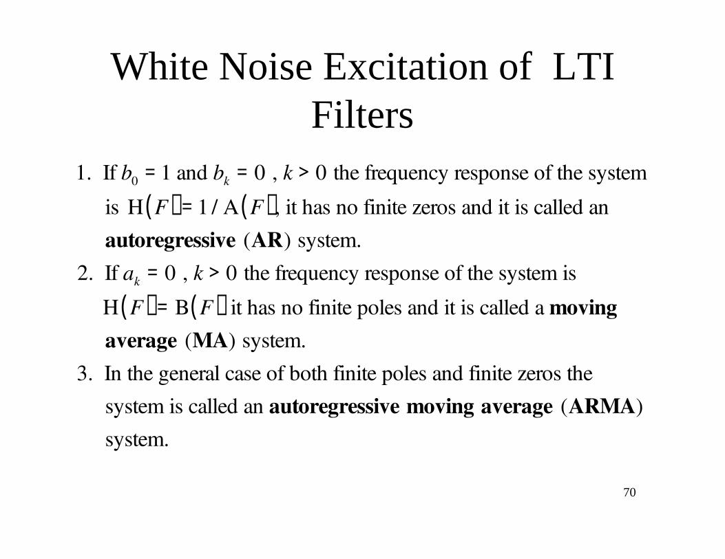
White Noise Excitation of LTI
Filters
1. If b0 = 1 and bk = 0 , k > 0 the frequency response of the system
is H F( ) = 1 / A F( ), it has no finite zeros and it is called an
autoregressive (AR) system.
2. If ak = 0 , k > 0 the frequency response of the system is
H F( ) = B F( ) it has no finite poles and it is called a moving
average (MA) system.
3. In the general case of both finite poles and finite zeros the
system is called an autoregressive moving average (ARMA)
system.

71
White Noise Excitation of LTI
Filters
If we multiply both sides of x n[ ]+ ak x n k[ ]k=1
p
= bkw n k[ ]k=0
q
by x* n + m[ ] and then take the expectation of both sides we get
R xx m[ ] = ak R xx m + k[ ]k=1
p
+ bk Rwx m + k[ ]k=0
q
.
Using x n[ ] = h n[ ] w n[ ] = h q[ ]w n q[ ]q=
we can show that
Rwx m[ ] = h m[ ] Rww m[ ] and, if w n[ ] is white noise
Rwx m[ ] = h m[ ] w2 m[ ] = w
2 h m[ ].
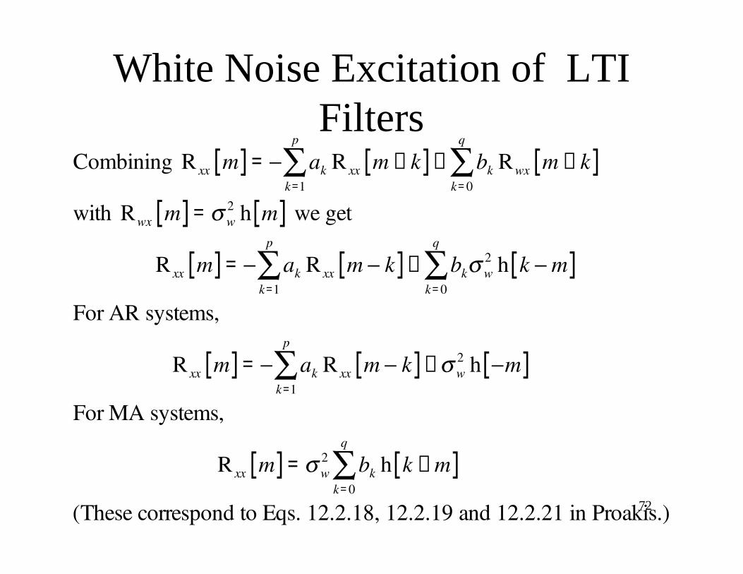
72
White Noise Excitation of LTI
FiltersCombining R xx m[ ] = ak R xx m + k[ ]
k=1
p
+ bk Rwx m + k[ ]k=0
q
with Rwx m[ ] = w2 h m[ ] we get
R xx m[ ] = ak R xx m k[ ]k=1
p
+ bk w2 h k m[ ]
k=0
q
For AR systems,
R xx m[ ] = ak R xx m k[ ]k=1
p
+ w2 h m[ ]
For MA systems,
R xx m[ ] = w2 bk h k + m[ ]
k=0
q
(These correspond to Eqs. 12.2.18, 12.2.19 and 12.2.21 in Proakis.)

73
White Noise Excitation of LTI
FiltersAn AR system with frequency response H F( ) =
1
1 0.2e j2 F
is excited by white noise with Rww m[ ] = w2 m[ ]. Find the
impulse response and autocorrelation of the output signal.
H z( ) =1
1 0.2e j2 F h n[ ] = 0.2n u n[ ]
Gxx F( ) = w2 H F( )H* F( ) = w
2 1
1 0.2e j2 F
1
1 0.2e j2 F
Gxx F( ) = w2
1 0.4cos 2 F( ) + 0.04R xx m[ ] = 1.042 w
2 0.2( )m
Example

74
White Noise Excitation of LTI
FiltersExample
R xx m[ ]R xx m 1[ ]
=1.042 w
2 0.2( )m
1.042 w2 0.2( )
m 1 =0.2( )
m
0.2( )m 1 = 0.2 , m > 0
Using the result for MA systems
R xx m[ ] = ak R xx m k[ ]k=1
p
+ w2 h m[ ]
R xx m[ ] = ak R xx m k[ ]k=1
p
, m > 0
R xx m[ ] = 0.2R xx m 1[ ]R xx m[ ]
R xx m 1[ ]= 0.2 , m > 0 Check.
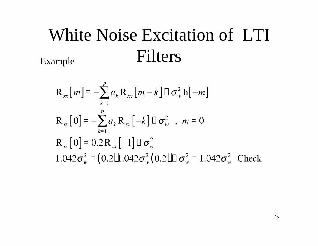
75
White Noise Excitation of LTI
FiltersExample
R xx m[ ] = ak R xx m k[ ]k=1
p
+ w2 h m[ ]
R xx 0[ ] = ak R xx k[ ]k=1
p
+ w2 , m = 0
R xx 0[ ] = 0.2R xx 1[ ]+ w2
1.042 w2
= 0.2( )1.042 w2 0.2( ) + w
2= 1.042 w
2 Check

76
White Noise Excitation of LTI
FiltersExample
R xx m[ ] = ak R xx m k[ ]k=1
p
+ w2 h m[ ] , m < 0
1.042 w2 0.2( )
m= 0.2 1.042 w
2 0.2( )m 1
+ w2 0.2( )
mu m[ ]
1.042 w2 0.2( )
m= 0.2 1.042 w
2 0.2( )1 m
+ w2 0.2( )
m
1.042 = 0.2 1.042 0.2 +1 = 1.042 Check
77
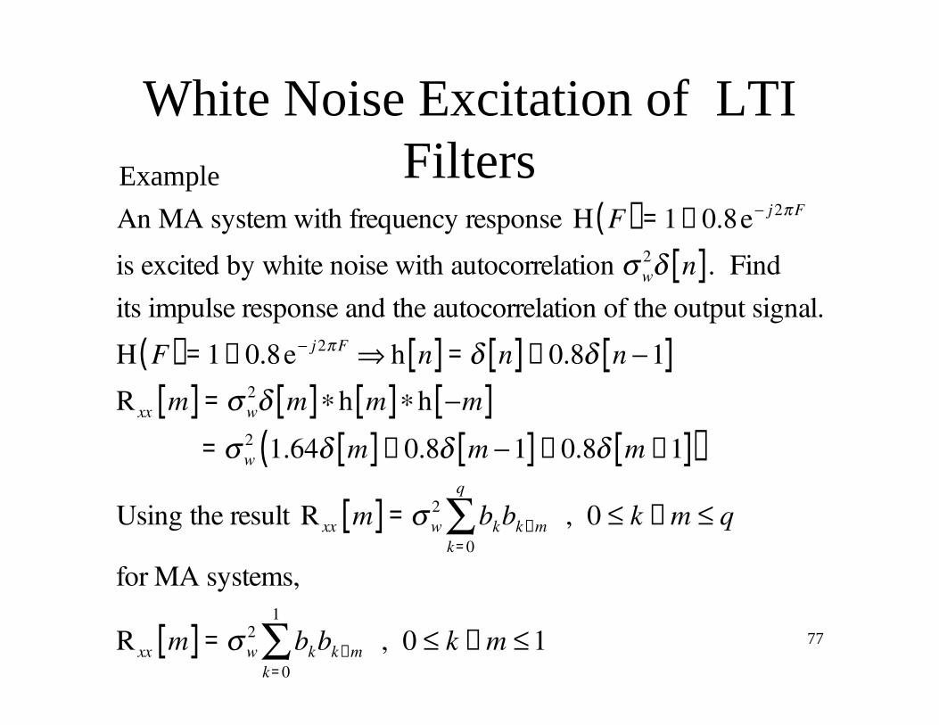
White Noise Excitation of LTI
FiltersExample
An MA system with frequency response H F( ) = 1+ 0.8e j2 F
is excited by white noise with autocorrelation w2 n[ ]. Find
its impulse response and the autocorrelation of the output signal.
H F( ) = 1+ 0.8e j2 F h n[ ] = n[ ]+ 0.8 n 1[ ]
R xx m[ ] = w2 m[ ] h m[ ] h m[ ]
= w2 1.64 m[ ]+ 0.8 m 1[ ]+ 0.8 m +1[ ]( )
Using the result R xx m[ ] = w2 bkbk+m
k=0
q
, 0 k + m q
for MA systems,
R xx m[ ] = w2 bkbk+m
k=0
1
, 0 k + m 1

78
White Noise Excitation of LTI
FiltersExample
R xx 0[ ] = w2 b0b0 + b1b1( ) = w
2 1+ 0.82( ) = 1.64 w2
R xx 1[ ] = w2 b0b1( ) = 0.8 w
2
R xx 1[ ] = w2 b1b0( ) = 0.8 w
2
Check.
79
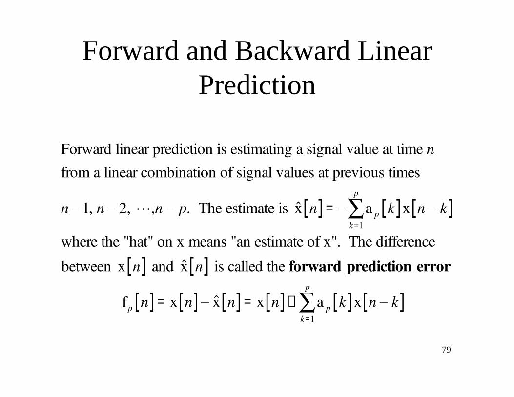
Forward and Backward Linear
Prediction
Forward linear prediction is estimating a signal value at time n
from a linear combination of signal values at previous times
n 1, n 2, ,n p. The estimate is x̂ n[ ] = a p k[ ]x n k[ ]k=1
p
where the "hat" on x means "an estimate of x". The difference
between x n[ ] and x̂ n[ ] is called the forward prediction error
fp n[ ] = x n[ ] x̂ n[ ] = x n[ ]+ a p k[ ]x n k[ ]k=1
p

80
Forward and Backward Linear
Prediction
A one-step forward linear predictor
81
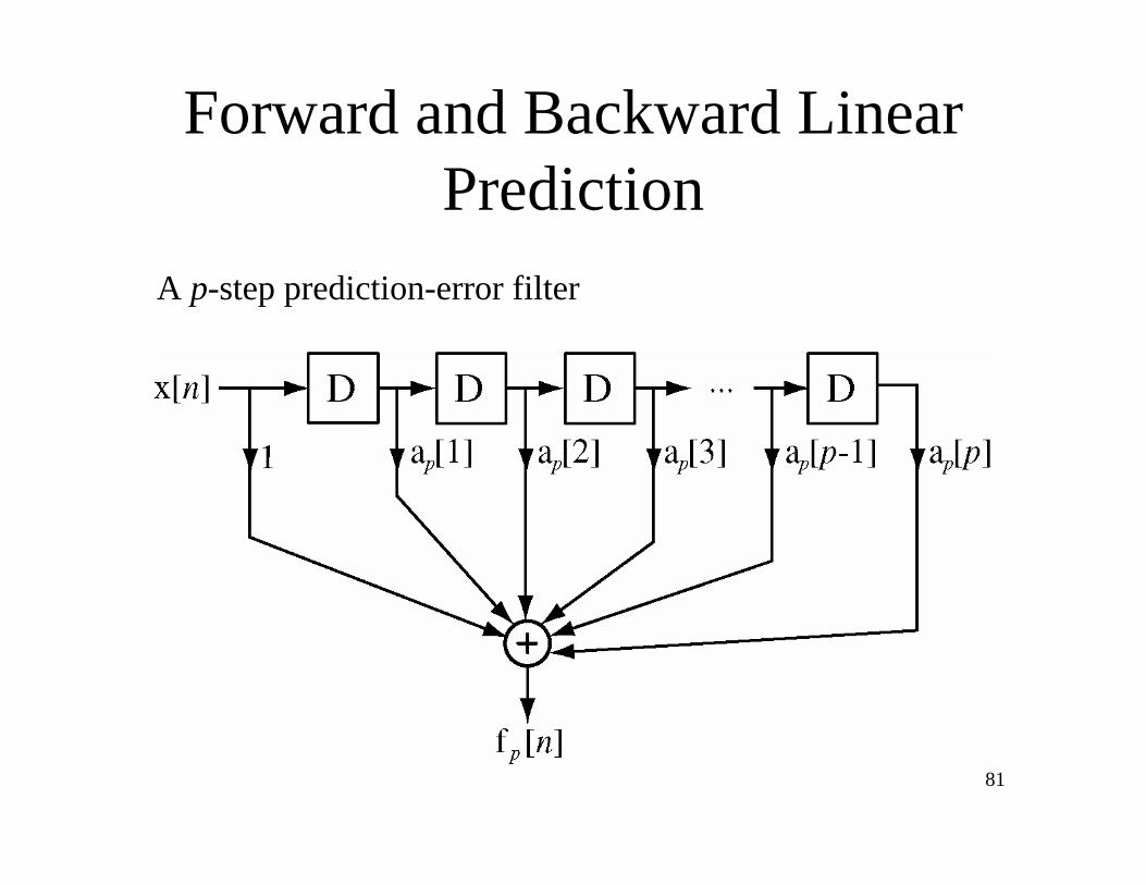
Forward and Backward Linear
Prediction
A p-step prediction-error filter

82
Forward and Backward Linear
PredictionA forward linear predictor can be realized as a lattice.
f0 n[ ] = g0 n[ ] = x n[ ]
fm n[ ] = fm 1 n[ ]+ Km gm 1 n 1[ ] , m = 0,1,2, , p
gm n[ ] = Km* fm 1 n[ ]+ gm 1 n 1[ ] , m = 0,1,2, , p
(Notice that the reflection coefficients are no longer identical in
a single stage but are instead complex conjugates. This is done
to handle the case of complex-valued signals.)

83
Forward and Backward Linear
Prediction
From chapter 9
0 z( ) = 0 z( ) = 1
m z( ) = m 1 z( ) + Kmz 1m 1 z( )
m z( ) = z mm 1 / z( )
m 1 z( ) = m z( ) Km m z( )1 Km
2
Km = m m[ ]
84
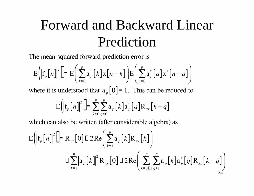
Forward and Backward Linear
PredictionThe mean-squared forward prediction error is
E fp n[ ]2
( ) = E a p k[ ]x n k[ ]k=0
p
E a p* q[ ]x* n q[ ]
q=0
p
where it is understood that a p 0[ ] = 1. This can be reduced to
E fp n[ ]2
( ) = a p k[ ]a p* q[ ]R xx k q[ ]
q=0
p
k=0
p
which can also be written (after considerable algebra) as
E fp n[ ]2
( ) = R xx 0[ ]+ 2Re a p k[ ]R xx k[ ]k=1
p
+ a p k[ ]2R xx 0[ ]
k=1
p
+ 2Re a p k[ ]a p* q[ ]R xx k q[ ]
q=1
p
k=q+1
p
85
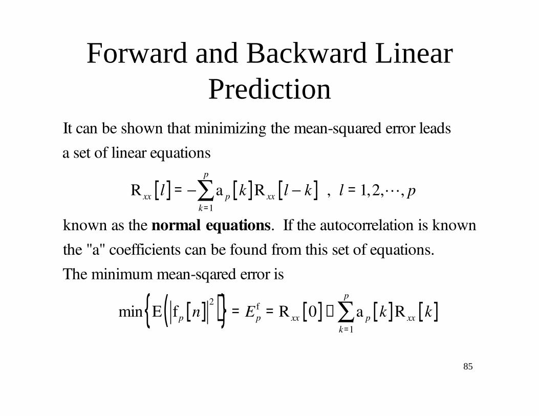
Forward and Backward Linear
Prediction
It can be shown that minimizing the mean-squared error leads
a set of linear equations
R xx l[ ] = a p k[ ]R xx l k[ ]k=1
p
, l = 1,2, , p
known as the normal equations. If the autocorrelation is known
the "a" coefficients can be found from this set of equations.
The minimum mean-sqared error is
min E fp n[ ]2
( ){ } = Epf
= R xx 0[ ]+ a p k[ ]R xx k[ ]k=1
p

86
Forward and Backward Linear
Prediction
We can also "predict" in the backward direction. We can estimate
x n p[ ] from the values of x n[ ] , x n 1[ ] , ,x n p +1[ ].
The estimate is
x̂ n p[ ] = bp k[ ]x n k[ ]k=0
p 1
and the backward "prediction" error is
gp n[ ] = x n p[ ]+ bp k[ ]x n k[ ]k=0
p 1
.
The minimum mean-squared error is the same as in the forward
prediction case
min E gp n[ ]2
( )( ) = Epg
= Epf
87
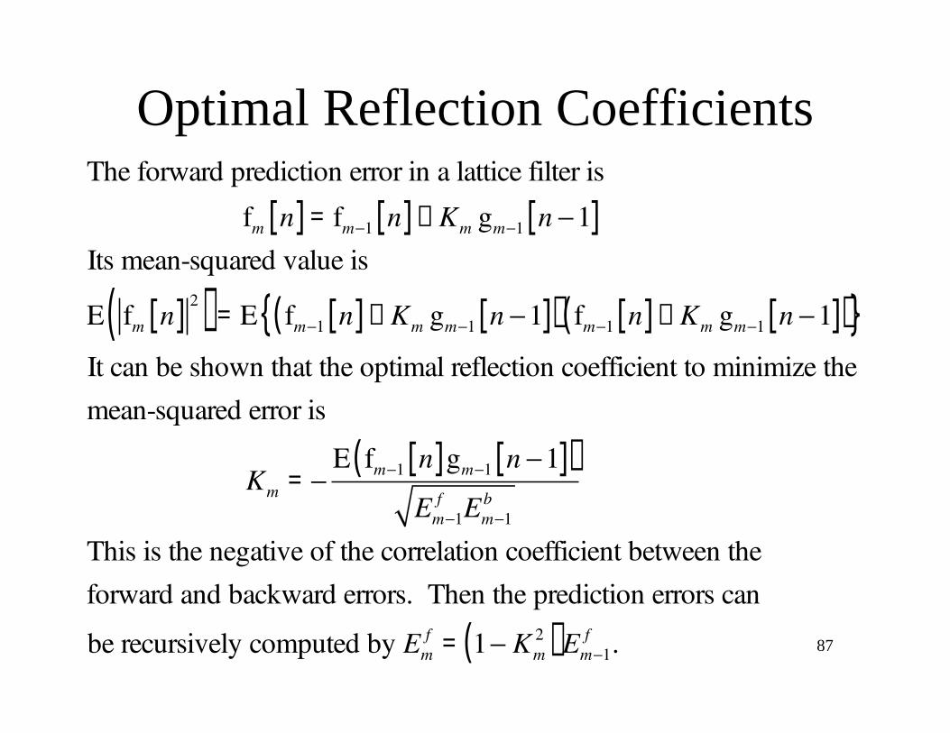
Optimal Reflection CoefficientsThe forward prediction error in a lattice filter is
fm n[ ] = fm 1 n[ ]+ Km gm 1 n 1[ ]Its mean-squared value is
E fm n[ ]2( ) = E fm 1 n[ ]+ Km gm 1 n 1[ ]( ) fm 1 n[ ]+ Km gm 1 n 1[ ]( ){ }
It can be shown that the optimal reflection coefficient to minimize the
mean-squared error is
Km =E fm 1 n[ ]gm 1 n 1[ ]( )
Em 1f Em 1
b
This is the negative of the correlation coefficient between the
forward and backward errors. Then the prediction errors can
be recursively computed by Emf
= 1 Km2( )Em 1
f .

88
AR Processes and Linear
Prediction
There is a one-to-one correspondence between the parameters in
an AR process and the predictor-coefficients of a p-th order
predictor. If the process is actually AR and pth order, they are the
same. If the output signal from an AR process excited by white
noise is applied to the corresponding predictor, the output signal
from the predictor will be white noise. So the prediction filter is
often called a “whitening” filter.

89
Properties of Linear Prediction-
Error Filters
It can be shown that if the reflection coefficients in a lattice-type
linear prediction-error filter are all less than one in magnitude, that
the zeros of A(z) all lie inside the unit circle. This makes A(z)
minimum-phase. All the zeros of B(z) lie outside the unit circle
making it maximum-phase.

90
Wiener FiltersBelow is a general system model for an optimal linear filter
called a Wiener filter. It makes the best estimate of d n[ ]based
on x n[ ], which contains a signal s n[ ] plus noise w n[ ], and
the autocorrelation functions for s n[ ] and w n[ ]. The estimation
error is e n[ ].
If d n[ ] = s n[ ], the estimation problem is called filtering.
If d n[ ] = s n + n0[ ] , n0 > 0, it is called prediction.
If d n[ ] = s n n0[ ] , n0 > 0, it is called smoothing.

91
Wiener Filters
The filter is optimized by minimizing the mean-squared
estimation error
E e n[ ]2( ) = E d n[ ] h m[ ]x n m[ ]
m=0
M 1 2
.
A set of equations called the Wiener - Hopf equations
h m[ ]R xx l m[ ]m=0
M 1
= Rdx l[ ] , l = 0,1, ,M 1
is used to find the impulse response of the optimal linear filter.
In Proakis' notation, h k( ) xx l k( )k=0
M 1
= dx l( ). The sign
difference on the right is caused by using a different definition
of autocorrelation. But both sets of equations yield an optimal
impulse response.
92
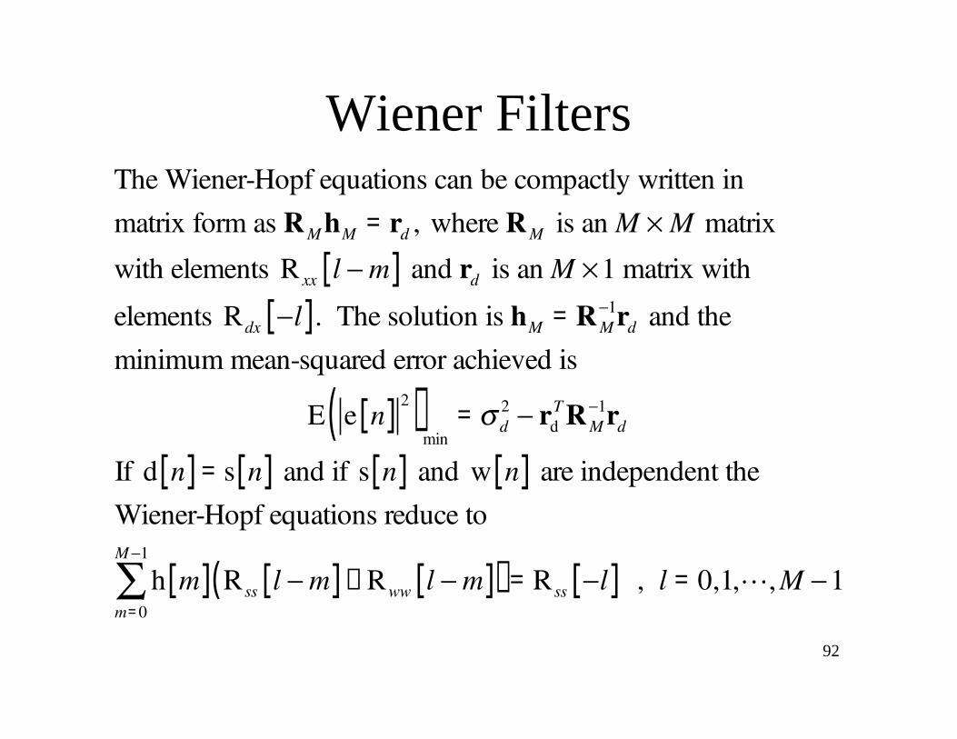
Wiener Filters
The Wiener-Hopf equations can be compactly written in
matrix form as RM hM = rd , where RM is an M M matrix
with elements R xx l m[ ] and rd is an M 1 matrix with
elements Rdx l[ ]. The solution is hM = RM1rd and the
minimum mean-squared error achieved is
E e n[ ]2( )
min= d
2 rdT RM
1rd
If d n[ ] = s n[ ] and if s n[ ] and w n[ ] are independent the
Wiener-Hopf equations reduce to
h m[ ] Rss l m[ ]+ Rww l m[ ]( )m=0
M 1
= Rss l[ ] , l = 0,1, , M 1
93
Wiener Filters
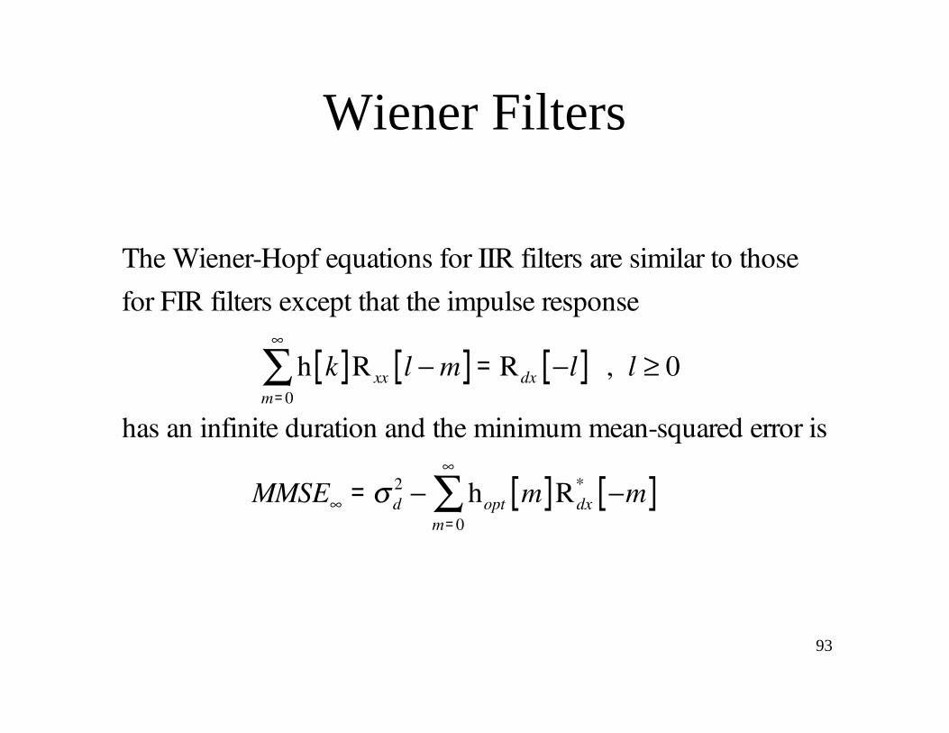
The Wiener-Hopf equations for IIR filters are similar to those
for FIR filters except that the impulse response
h k[ ]R xx l m[ ]m=0
= Rdx l[ ] , l 0
has an infinite duration and the minimum mean-squared error is
MMSE = d2 hopt m[ ]Rdx
* m[ ]m=0
94
Wiener Filters
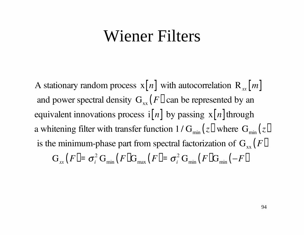
A stationary random process x n[ ] with autocorrelation R xx m[ ]
and power spectral density Gxx F( ) can be represented by an
equivalent innovations process i n[ ] by passing x n[ ] through
a whitening filter with transfer function 1 / Gmin z( ) where Gmin z( )
is the minimum-phase part from spectral factorization of Gxx F( )
Gxx F( ) = i2 Gmin F( )Gmax F( ) = i
2 Gmin F( )Gmin F( )
95
Wiener Filters
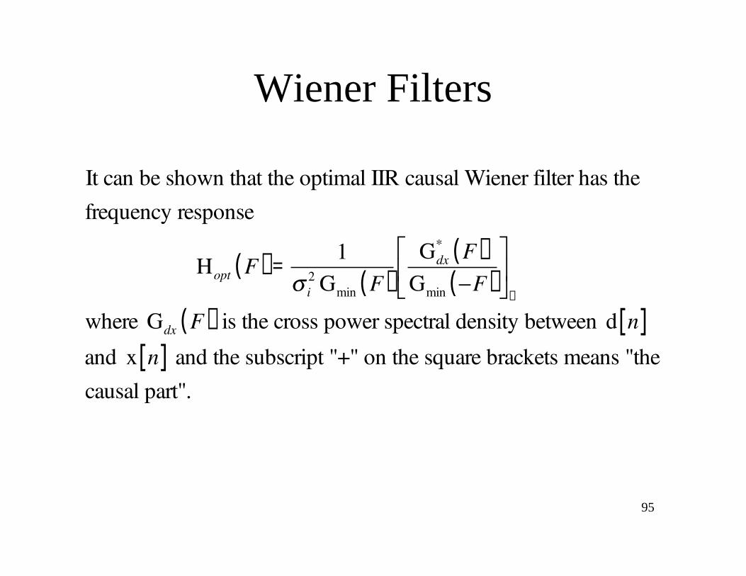
It can be shown that the optimal IIR causal Wiener filter has the
frequency response
Hopt F( ) =1
i2 Gmin F( )
Gdx* F( )
Gmin F( )+
where Gdx F( ) is the cross power spectral density between d n[ ]
and x n[ ] and the subscript "+" on the square brackets means "the
causal part".

96
Wiener FiltersIIR Wiener Filter Example (An extension of Example 12.7.2 in Proakis)
Let x n[ ] = s n[ ]+ w n[ ] where s n[ ] is an AR process that
satisfies the equation s n[ ] = 0.6s n 1[ ]+ v n[ ] where v n[ ]
is a white noise sequence with variance v2
= 0.64 and w n[ ]
is a white noise sequency with variance w2
= 1. Design a
Wiener filter to optimally estimate the signal s n[ ] and delayed
versions of the signal s n n0[ ].
The system impulse response is h n[ ] = 0.6( )n
u n[ ] and the
transfer function is H z( ) =1
1 0.6z 1 =z
z 0.6.

97
Wiener FiltersIIR Wiener Filter Example (An extension of Example 12.7.2 in Proakis)
The power spectral density of s n[ ] is
Gss z( ) = Gvv z( ) H z( )2
= v2 H z( )
2
= 0.641
1 0.6z 1
1
1 0.6z=
0.64
1.36 0.6 z 1+ z( )
The power spectral density of x n[ ] is
Gxx z( ) = Gss z( ) + Gww z( ) =0.64
1.36 0.6 z 1+ z( )
+1 =2 0.6 z 1
+ z( )1.36 0.6 z 1
+ z( )This can be spectrally factored into the form
Gxx z( ) =a bz 1( ) a bz( )
1 0.6z 1( ) 1 0.6z( )
98
Wiener FiltersIIR Wiener Filter Example (An extension of Example 12.7.2 in Proakis)
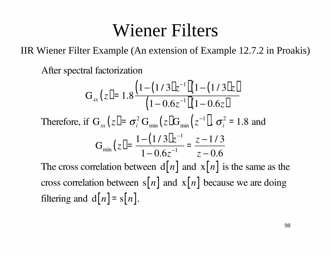
After spectral factorization
Gxx z( ) = 1.81 1 / 3( )z 1( ) 1 1 / 3( )z( )
1 0.6z 1( ) 1 0.6z( )
Therefore, if Gxx z( ) = i2 Gmin z( )Gmin z 1( ), i
2= 1.8 and
Gmin z( ) =1 1 / 3( )z 1
1 0.6z 1 =z 1 / 3
z 0.6The cross correlation between d n[ ] and x n[ ] is the same as the
cross correlation between s n[ ] and x n[ ] because we are doing
filtering and d n[ ] = s n[ ].

99
Wiener FiltersIIR Wiener Filter Example (An extension of Example 12.7.2 in Proakis)
Rdx m[ ] = Rsx m[ ] = E s n[ ]x n + m[ ]( ) = E s n[ ] s n + m[ ]+ w n + m[ ]( )( )Rdx m[ ] = E s n[ ]s n + m[ ]( ) + E s n[ ]w n + m[ ]( ) = Rss m[ ]+ Rsw m[ ]
=0
= Rss m[ ]
Therefore Gdx z( ) = Gss z( ) =0.64
1.36 0.6 z 1+ z( )
=0.64
1 0.6z 1( ) 1 0.6z( )
and Gdx z 1( )Gmin z 1( )
+
=
0.64
1 0.6z( ) 1 0.6z 1( )1 1 / 3( )z
1 0.6z+
=0.64
1 1 / 3( )z( ) 1 0.6z 1( )+
100
Wiener FiltersIIR Wiener Filter Example (An extension of Example 12.7.2 in Proakis)
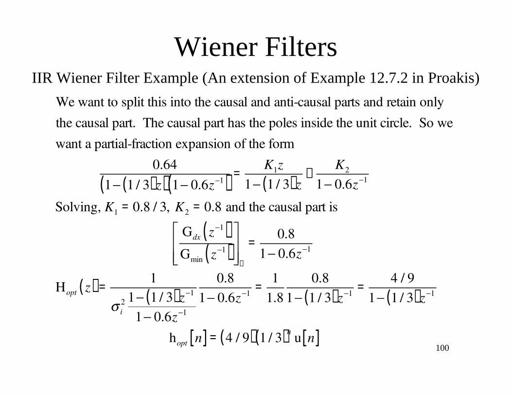
We want to split this into the causal and anti-causal parts and retain only
the causal part. The causal part has the poles inside the unit circle. So we
want a partial-fraction expansion of the form
0.64
1 1 / 3( )z( ) 1 0.6z 1( )=
K1z
1 1 / 3( )z+
K2
1 0.6z 1
Solving, K1 = 0.8 / 3, K2 = 0.8 and the causal part is
Gdx z 1( )Gmin z 1( )
+
=0.8
1 0.6z 1
Hopt z( ) =1
i2 1 1 / 3( )z 1
1 0.6z 1
0.8
1 0.6z 1 =1
1.8
0.8
1 1 / 3( )z 1 =4 / 9
1 1 / 3( )z 1
hopt n[ ] = 4 / 9( ) 1 / 3( )n
u n[ ]
101
Wiener FiltersIIR Wiener Filter Example (An extension of Example 12.7.2 in Proakis)
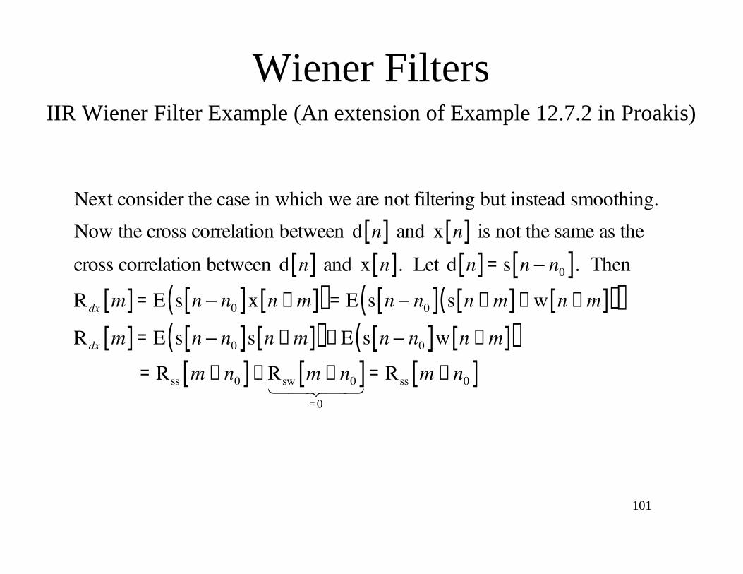
Next consider the case in which we are not filtering but instead smoothing.
Now the cross correlation between d n[ ] and x n[ ] is not the same as the
cross correlation between d n[ ] and x n[ ]. Let d n[ ] = s n n0[ ]. Then
Rdx m[ ] = E s n n0[ ]x n + m[ ]( ) = E s n n0[ ] s n + m[ ]+ w n + m[ ]( )( )Rdx m[ ] = E s n n0[ ]s n + m[ ]( ) + E s n n0[ ]w n + m[ ]( ) = Rss m + n0[ ]+ Rsw m + n0[ ]
=0
= Rss m + n0[ ]
102
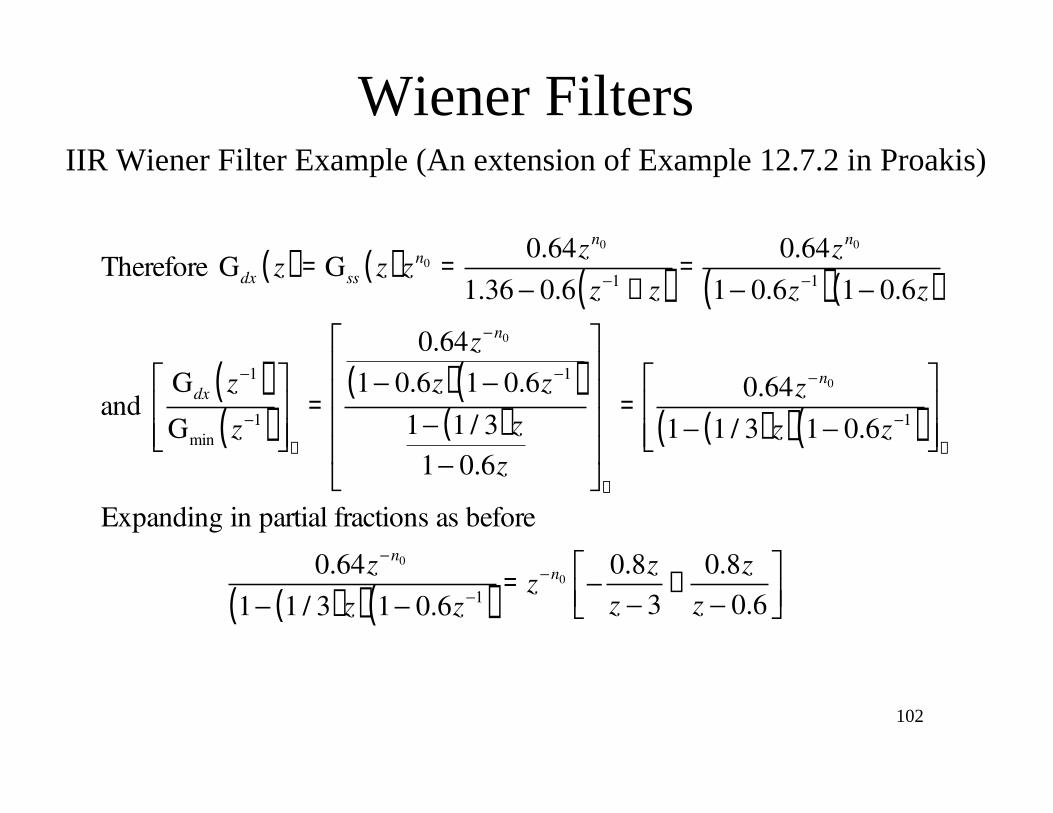
Wiener FiltersIIR Wiener Filter Example (An extension of Example 12.7.2 in Proakis)
Therefore Gdx z( ) = Gss z( )zn0 =0.64zn0
1.36 0.6 z 1+ z( )
=0.64zn0
1 0.6z 1( ) 1 0.6z( )
and Gdx z 1( )Gmin z 1( )
+
=
0.64z n0
1 0.6z( ) 1 0.6z 1( )1 1 / 3( )z
1 0.6z+
=0.64z n0
1 1 / 3( )z( ) 1 0.6z 1( )+
Expanding in partial fractions as before
0.64z n0
1 1 / 3( )z( ) 1 0.6z 1( )= z n0
0.8z
z 3+
0.8z
z 0.6

103
Wiener FiltersIIR Wiener Filter Example (An extension of Example 12.7.2 in Proakis)
0.8 3( )n
u n +1( ) + 0.8 0.6( )n
u n[ ] Z 0.8z
z 3+
0.8z
z 0.6
0.8 3( )n n0 u n n0 +1( ) + 0.8 0.6( )
n n0 u n n0[ ] Z z n00.8z
z 3+
0.8z
z 0.6The causal part of the inverse transform is
0.8 3( )n n0 u n n0 +1( ) + 0.8 0.6( )
n n0 u n n0[ ]{ }u n[ ]
which can be written as
0.8 3( )n n0 u n[ ] u n n0[ ]( ) + 0.8 0.6( )
n n0 u n n0[ ]Its z transform is
0.81
3
3( )n0 z n0
1 / 3( ) z 1 +z n0
1 0.6z 1

104
Wiener FiltersIIR Wiener Filter Example (An extension of Example 12.7.2 in Proakis)
Gdx z 1( )Gmin z 1( )
+
= 0.8 / 3( )1 / 3( )
n0 z n0
1 / 3 z 1 +0.8z n0
1 0.6z 1
Hopt z( ) =1
i2 1 1 / 3( )z 1
1 0.6z 1
0.8 / 3( )1 / 3( )
n0 z n0
1 / 3( ) z 1 +0.8z n0
1 0.6z 1
which can be written as
Hopt z( ) =5
9z n0 1( ) 0.8 / 3( ) 1 / 3( )
n0 1 z 0.6
z 1 / 3
zn0 3( )n0
z 3+
0.8
z 1 / 3

105
Wiener FiltersIIR Wiener Filter Example (An extension of Example 12.7.2 in Proakis)
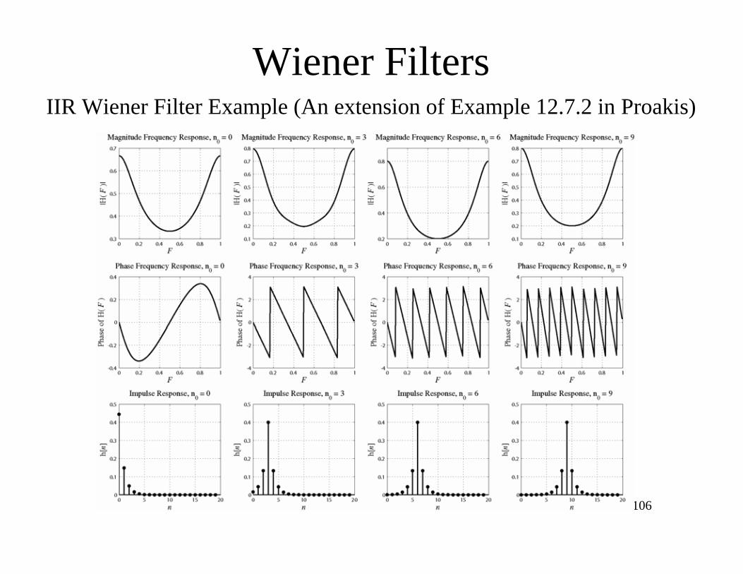
The impulse response of the filter is the inverse transform of this transfer
function. Finding a general expression for it is very tedious. But we can
see its form by finding the frequency response
Hopt e j( ) =5
9e j n0 1( ) 0.8 / 3( ) 1 / 3( )
n0 1 e j 0.6
e j 1 / 3
e j n0 3( )n0
e j 3+
0.8
e j 1 / 3
and then computing the impulse response numerically, using the fast Fourier
transform.
106
Wiener FiltersIIR Wiener Filter Example (An extension of Example 12.7.2 in Proakis)
107
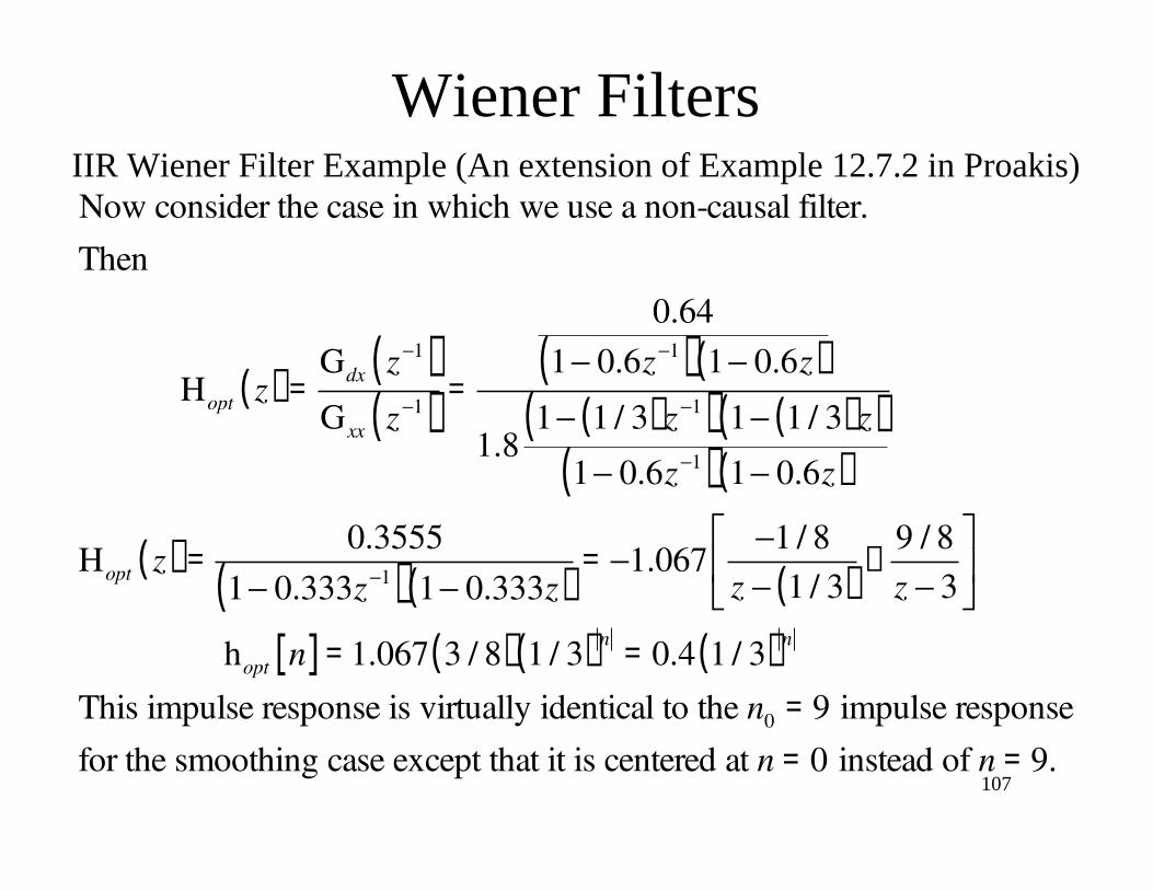
Wiener FiltersIIR Wiener Filter Example (An extension of Example 12.7.2 in Proakis)
Now consider the case in which we use a non-causal filter.
Then
Hopt z( ) =Gdx z 1( )Gxx z 1( )
=
0.64
1 0.6z 1( ) 1 0.6z( )
1.81 1 / 3( )z 1( ) 1 1 / 3( )z( )
1 0.6z 1( ) 1 0.6z( )
Hopt z( ) =0.3555
1 0.333z 1( ) 1 0.333z( )= 1.067
1 / 8
z 1 / 3( )+
9 / 8
z 3
hopt n[ ] = 1.067 3 / 8( ) 1 / 3( )n
= 0.4 1 / 3( )n
This impulse response is virtually identical to the n0 = 9 impulse response
for the smoothing case except that it is centered at n = 0 instead of n = 9.