efficient seakeeping performance predictions with...

IN DEGREE PROJECT VEHICLE ENGINEERING,SECOND CYCLE, 30 CREDITS

, STOCKHOLM SWEDEN 2019

Efficient seakeeping performance predictions with CFD

BENJAMIN LAGEMANN

KTH ROYAL INSTITUTE OF TECHNOLOGYSCHOOL OF ENGINEERING SCIENCES

E�cient seakeeping performance predictions with CFD

Benjamin LagemannTRITA TRITA-SCI-GRU 2019:290

Degree Project in Mechanical Engineering, Second Cycle, 30 CreditsCourse SD271X, Degree Project in Naval Architecture

Stockholm, Sweden 2019School of Engineering SciencesKTH Royal Institute of TechnologySE-100 44, StockholmSweden Telephone: +46 8 790 60 00

Front cover illustration: Visualization of performed seakeeping simulation in FINE�/Marine

Preface

This thesis marks the end of my joint master studies at Norwegian Institute of Science and Technology(NTNU) in Trondheim and Royal Institute of Technology (KTH) in Stockholm. It has been a greatpleasure to study at both these universities and - not only but also thanks to Paul Anderson -coordination and complementation within the Maritime Engineering study track worked very well.Thanks to the close collaboration between the Nordic5Tech universities, I received the opportunity tovisit Chalmers University of Technology and to work on an interesting and challenging thesis projectat SSPA Gothenburg. At this point, I would like to thank the entire team of SSPA Gothenburg fortheir support and convenient collaboration. In particular, I want to express my gratitude to BurakKorkmaz, who provided me with excellent support on usage of CFD software, Martin Kjellberg for hisvaluable advice on seakeeping simulations and So�a Werner for de�ning the project scope and givingme the opportunity to work on this subject.Also, I would like to thank my co-supervisor Håvard Holm (NTNU) for his assistance with literaturereview and �nding comparative data.Finally, I want to thank my supervisor Hans Liwång (KTH) for his great support and valuable feedbackon my work throughout this thesis.

Gothenburg, July 2019

Benjamin Lagemann

II

Abstract

With steadily increasing computational power, computational �uid dynamics (CFD) can be appliedto unsteady problems such as seakeeping simulations. Therefore, a good balance between accuracyand computational speed is required. This thesis investigates the application of CFD to seakeepingperformance predictions and aims to propose a best-practice procedure for e�cient seakeeping simu-lations.The widely used KVLCC2 research vessel serves as a test case for this thesis and FINE�/Marine

software package is used for CFD computations. In order to validate the simulations, results arecompared to recent experimental data from SSPA as well as predictions with potential �ow codeSHIPFLOW® Motions.As for the calm water simulations, both inviscid and viscous �ow computations are performed in

combination with three mesh re�nement levels.Seakeeping simulations with regular head waves of di�erent wavelengths are set-up correspondingly.

Furthermore, di�erent strategies for time discretization are investigated. With the given computationalresources, it is not feasible to complete seakeeping simulations with a �ne mesh. However, already thecoarse meshes give good agreement to experiments and SHIPFLOW® Motions' predictions. Viscous�ow simulations turn out to be more robust than Euler �ow computations and thus should be preferred.Regarding the time discretization, a �xed time discretization of 150 steps per wave period has shownthe best balance between accuracy and speed. Based on these �ndings, a best-practice procedure forseakeeping performance predictions in FINE�/Marine is established.Taking the most e�cient settings obtained from head wave simulations, the vessel is subjected

to oblique waves with 160° encounter angle. Under similar wave conditions, CFD predictions of asimilar thesis show close agreement in terms of added wave resistance. Compared to the previoushead wave conditions of this study, added resistance in 160° oblique waves is found to be signi�cantlyhigher. This underlines that oblique bow quartering waves represent a relevant case for determiningthe maximum required power of a ship.CFD and potential �ow show similar accuracy with respect to ship motions and added wave resis-

tance, albeit potential �ow outperforms CFD in terms of computational speed. Hence, CFD shouldbe applied in cases where viscous e�ects are known to have large in�uence on a vessel's seakeepingbehavior. This can be the case if motion control and damping devices are to be evaluated, for instance.

Key words: added wave resistance, CFD, Courant-adapted time step, Euler �ow, FINE�/Marine,inviscid �ow, k-ω SST-Menter, KVLCC2, RANS, regular waves, seakeeping, sub-cycling acceleration,time discretization, viscous �ow

III

Sammanfattning

Tack vare den stadigt ökande beräkningskraften kan beräknings�uiddynamik (CFD) idag användas påberäkningsintensiva problem som sjöegenskapssimulationer. Den här rapporten undersöker användningav CFD på sjöegenskapsprestanda och syftar till att foreslå ett best-practice förfaringssätt för e�ektivsjöegenskapssimulationer.Forskningsskrovet KVLCC2 fungerar som ett testfall för denna rapport och FINE�/Marine-mjukvarupaketet

används för CFD-beräkningar. Viktiga parametrar, såsom �ödestyp, beräkningsnät och tidssteg varie-rars systematiskt. Resultaten jämförs med experiment gjorda vid SSPA. Baserat på resultaten förelåsen best-practice.Den föreslagna best-practice användas vidare för berökningar av sjöegenskaper i sneda vågor. Jäm-

förelse av resultaten med liknande studier visar god överensstämmelse.Genom att använda det föreslagna förfarandet för best-practice kan CFD-sjöegenskapssimulationer

användas på fall där viskösa krafter måste beaktas, till exempel rörelseregleringsanordningar.

IV

Contents

Abstract III

Sammanfattning IV

1 Introduction 1

2 Theory 2

2.1 Resistance and seakeeping performance . . . . . . . . . . . . . . . . . . . . . . . . . 22.1.1 Calm water and added wave resistance . . . . . . . . . . . . . . . . . . . . . 22.1.2 Methods for calculating the added wave resistance . . . . . . . . . . . . . . . 2

2.1.2.1 Analytical and semi-empirical methods . . . . . . . . . . . . . . . . 22.1.2.2 Potential �ow methods . . . . . . . . . . . . . . . . . . . . . . . . 32.1.2.3 Computational �ow methods . . . . . . . . . . . . . . . . . . . . . 52.1.2.4 Model tests . . . . . . . . . . . . . . . . . . . . . . . . . . . . . . 5

2.2 Computational �uid dynamics . . . . . . . . . . . . . . . . . . . . . . . . . . . . . . 62.2.1 Reynolds-averaged Navier-Stokes equations . . . . . . . . . . . . . . . . . . 6

2.2.1.1 Turbulence modeling . . . . . . . . . . . . . . . . . . . . . . . . . 72.2.1.2 Boundary layers . . . . . . . . . . . . . . . . . . . . . . . . . . . . 7

2.2.2 Euler method . . . . . . . . . . . . . . . . . . . . . . . . . . . . . . . . . . 82.2.3 Discretization of computational domain and free surface capturing . . . . . . 9

3 Methodology and computational set-up 10

3.1 Methods investigated in this thesis . . . . . . . . . . . . . . . . . . . . . . . . . . . 103.2 Model description . . . . . . . . . . . . . . . . . . . . . . . . . . . . . . . . . . . . 103.3 Computational set-up . . . . . . . . . . . . . . . . . . . . . . . . . . . . . . . . . . 11

3.3.1 Meshing . . . . . . . . . . . . . . . . . . . . . . . . . . . . . . . . . . . . . 113.3.1.1 Computational domain . . . . . . . . . . . . . . . . . . . . . . . . 123.3.1.2 Subdivision of computational domain . . . . . . . . . . . . . . . . 133.3.1.3 Viscous layers . . . . . . . . . . . . . . . . . . . . . . . . . . . . . 14

3.3.2 Multi-�uid model . . . . . . . . . . . . . . . . . . . . . . . . . . . . . . . . 143.3.2.1 Flow model . . . . . . . . . . . . . . . . . . . . . . . . . . . . . . 14

3.3.3 Boundary conditions . . . . . . . . . . . . . . . . . . . . . . . . . . . . . . . 143.3.3.1 Wave generation . . . . . . . . . . . . . . . . . . . . . . . . . . . 14

3.3.4 Body motions . . . . . . . . . . . . . . . . . . . . . . . . . . . . . . . . . . 153.3.5 Mesh management . . . . . . . . . . . . . . . . . . . . . . . . . . . . . . . 163.3.6 Wave damping zones . . . . . . . . . . . . . . . . . . . . . . . . . . . . . . 163.3.7 Time discretization and computational control . . . . . . . . . . . . . . . . . 173.3.8 Output and post-processing . . . . . . . . . . . . . . . . . . . . . . . . . . . 17

V

Contents

3.3.8.1 Post-processing of calm water simulations . . . . . . . . . . . . . . 183.3.8.2 Post-processing of seakeeping simulation . . . . . . . . . . . . . . . 183.3.8.3 Subtraction of calm water resistance from total resistance . . . . . 20

3.4 Parameters to be investigated . . . . . . . . . . . . . . . . . . . . . . . . . . . . . . 203.5 Computational resources . . . . . . . . . . . . . . . . . . . . . . . . . . . . . . . . . 21

4 Results and discussion 22

4.1 Wave study . . . . . . . . . . . . . . . . . . . . . . . . . . . . . . . . . . . . . . . 224.2 Mesh veri�cation study . . . . . . . . . . . . . . . . . . . . . . . . . . . . . . . . . 24

4.2.1 Calm water resistance . . . . . . . . . . . . . . . . . . . . . . . . . . . . . . 244.2.2 Coarse mesh . . . . . . . . . . . . . . . . . . . . . . . . . . . . . . . . . . . 254.2.3 Medium mesh . . . . . . . . . . . . . . . . . . . . . . . . . . . . . . . . . . 274.2.4 Fine mesh . . . . . . . . . . . . . . . . . . . . . . . . . . . . . . . . . . . . 29

4.3 Inviscid �ow simulation . . . . . . . . . . . . . . . . . . . . . . . . . . . . . . . . . 304.4 Courant-adapted time step . . . . . . . . . . . . . . . . . . . . . . . . . . . . . . . 324.5 Final choice of time step . . . . . . . . . . . . . . . . . . . . . . . . . . . . . . . . 344.6 Oblique waves . . . . . . . . . . . . . . . . . . . . . . . . . . . . . . . . . . . . . . 36

4.6.1 Comparison with CFD calculations of a thesis study at NTNU . . . . . . . . 374.6.2 Comparison with head waves . . . . . . . . . . . . . . . . . . . . . . . . . . 38

5 Conclusions 40

5.1 Recommendation of best-practice procedure . . . . . . . . . . . . . . . . . . . . . . 415.2 Suggestions for further work . . . . . . . . . . . . . . . . . . . . . . . . . . . . . . . 42

Nomenclature 46

References 47

Appendix a

VI

1 Introduction

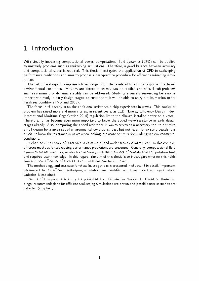
With steadily increasing computational power, computational �uid dynamics (CFD) can be appliedto unsteady problems such as seakeeping simulations. Therefore, a good balance between accuracyand computational speed is required. This thesis investigates the application of CFD to seakeepingperformance predictions and aims to propose a best-practice procedure for e�cient seakeeping simu-lations.The �eld of seakeeping comprises a broad range of problems related to a ship's response to external

environmental conditions. Motions and forces in seaway can be studied and special sub-problemssuch as slamming or dynamic stability can be addressed. Studying a vessel's seakeeping behavior isimportant already in early design stages, to ensure that it will be able to carry out its mission underharsh sea conditions (Molland 2008).The focus in this study is on the additional resistance a ship experiences in waves. This particular

problem has raised more and more interest in recent years, as EEDI (Energy E�ciency Design Index,International Maritime Organization 2014) regulation limits the allowed installed power on a vessel.Therefore, it has become even more important to know the added wave resistance in early designstages already. Also, computing the added resistance in waves serves as a necessary tool to optimizea hull design for a given set of environmental conditions. Last but not least, for existing vessels it iscrucial to know the resistance in waves when looking into route optimization under given environmentalconditions.In chapter 2 the theory of resistance in calm water and under seaway is introduced. In this context,

di�erent methods for seakeeping performance predictions are presented. Generally, computational �uiddynamics are assumed to give very high accuracy with the drawback of considerable computation timeand required user knowledge. In this regard, the aim of this thesis is to investigate whether this holdstrue and how e�ciency of such CFD computations can be improved.The methodology and test case for these investigations is presented in chapter 3 in detail. Important

parameters for an e�cient seakeeping simulation are identi�ed and their choice and systematicalvariation is explained.Results of this parameter study are presented and discussed in chapter 4. Based on these �n-

dings, recommendations for e�cient seakeeping simulations are drawn and possible user scenarios aredetected (chapter 5).

1

2 Theory

2.1 Resistance and seakeeping performance

The topic of seakeeping addresses many aspects of a vessel in seaway, such as ship motions andoccurrence of slamming, propeller performance in waves, impact of sea conditions on structural designor ship stability in waves (Bertram 2012a). As this study focuses on the added wave resistance,di�erent methods for prediction of the ship resistance in waves are presented in this chapter. Theoverview starts with simple �rst-principle methods and goes on to the more advanced methods.

2.1.1 Calm water and added wave resistance

In model testing, bare hull ship resistance is traditionally split into viscous resistance Rv = (1 + k)Rf ,wave-making resistance Rw and air resistance Ra according to International Towing Tank Conference(2008). As the latter one is relatively small compared to the other parts, it is often neglected in theanalysis of model tests. The total calm water resistance is then composed as

RT,calm = (1 + k)Rf +Rw (2.1)

When measuring the resistance in waves, one will not only observe oscillatory forces, but also (in caseof head waves) a higher mean resistance force RT . Thus, the resistance can be expressed as

RT,waves = (1 + k)Rf +Rw +Raw (2.2)

with Raw = RT,waves − RT,calm being the added resistance due to incident waves. Alike the towingforce RT , the added wave resistance can be expressed by means of a non-dimensional coe�cient

Caw =Raw

ρgA2B2/L(2.3)

according to Larsson, Stern, and Visonneau (2014). However, regarding the added resistance in wavesit is not always easy to say whether viscous or pressure e�ects in�uence or even dominate the behavior.

2.1.2 Methods for calculating the added wave resistance

2.1.2.1 Analytical and semi-empirical methods

Empirical methods exist for many years and serve as a rough estimate for the added resistance inwaves. One of the oldest empirical formulas dates back to Kreitner 1939:

Raw = 0.64gH2sB

2Cbρ1

Lwl

(2

3+

1

3cosβ

)(2.4)

which gives an estimate on the added resistance based on ship's main particulars, signi�cant waveheight Hs and the wave encounter angle β.

2

CHAPTER 2. THEORY

It would be a wrong conclusion to assume that such simple methods are outdated. Recently,Boom, Huisman, and Mennen (2013) developed a method to correct sea trial resistance by addedwave resistance. The added resistance in waves, according to their proposal, should be calculatedempirically as

Raw = − 1

16ρgH2

sB

√B

Lb(2.5)

The above-mentioned formulas are usually valid for relatively short wave lengths. As this is commonlythe case for sea trials which are conducted in relatively, but not completely calm water, the methodproposed by Boom, Huisman, and Mennen (2013) was included into the ISO 15016 standard (2015) aswell as in the recommended procedures and guidelines of the ITTC committee (International TowingTank Conference 2014a).

2.1.2.2 Potential �ow methods

Alike the analytical and semi-empirical methods, numerical potential �ow methods have been appliedfor many years to seakeeping problems. All types of potential �ow-methods have in common, that thewater �uid is idealized as incompressible, irrotational and inviscid. Within potential �ow methods, theboundary conditions (i.e. a ship's hull surface for instance) can be modeled by means of a superpositionof sources, dipoles and vortices. Potential �ow methods can consider the local geometry of the vesselinstead of its main particulars. There are, on the other hand, considerable limitations to such methods.

Far �eld Maruo (1960) developed a method to estimate the added waves resistance based onthe potential of the incident waves in relation to the re�ected and transmitted waves of a body. Heassumes zero energy �ux to the body and thus concludes that

ζ2 = A2R +A2

T (2.6)

with the incident wave amplitude ζ, re�ected wave amplitude AR and transmitted wave amplitudeAT . The mean force acting on the body, can also be computed by means of the radiated waveamplitude A (θ) far away from the body as

F1 =ρg

4

ˆ 2π

0A2 (θ) (cosβ − cos θ) dθ (2.7)

Maruo's formula 2.7 has also been extended by Longuet-Higgins (1977) for �nite water depth. Later,the method has been expanded for more general vessel shapes by Gerritsma and Beukelman (1972).

Direct pressure integration Direct pressure integration has �rst been used introduced by Pink-ster and Oortmerssen (1977) and extended by Faltinsen et al. (1980) to include arbitrary waterplaneshapes as well as forward speed. It is applicable to derive the added resistance in short waves and forsmall Froude numbers Fn ≤ 0.2:

F1

ζ2a=

1

2ρg

(1 +

2ω0U

g

)ˆL1

sin2 θ · n1 dl (2.8)

This formula, however, is only valid for blunt bodies with vertical side walls in short waves and hencenot applicable for all types for vessels and waves.

3

CHAPTER 2. THEORY

Figure 2.1: Wave propagation and shadow region according to Faltinsen (1990)

Strip theory Strip theory assumes that a ship is slender, i.e. it is much longer than wide or deep.For this reason, the �ow is assumed to vary mostly in the cross-sectional plane. Visually speaking,the ship is therefore cut in thin cross-sections as shown in the picture below.

Figure 2.2: Hull divided into 2-dimensional sections according to strip theory (from Faltinsen 1990)

The calculation of �ow and forces for each cross-section can be based on analytical expressionsfor Lewis sections or numerically by means of two-dimensional panel methods (Bertram 2012a). Acommonly used implementation of this method has been proposed by Salvesen, Tuck, and Faltinsen(1970).Although the strip method is most applicable for slender hull forms, it does not work for planing

hulls. Therefore, a so-called 2,5-D extension for high-speed vessels has been presented by Chapman(1975). This method includes the information of upstream computations for a given cross-section,but assumes no downstream of information.

Panel Methods Panel methods discretize the hull surface into small panels (patches) and thuscan capture the 3D geometry of a vessel. As the �ow is assumed to be of potential type, the hullis modeled by sources of unknown strength that are assigned to the panels. In principle, one candistinguish between Green's Function Methods and Rankine Singularity Methods:While Green's Function Methods distribute sources on the average wetted surface, Rankine Sin-

gularity Methods also apply boundary conditions to the free surface. According to Bertram (2012a),Rankine Singularity Methods are generally preferable over Green's function Methods, albeit beingslightly more complicated to implement.As panel methods assume potential �ow, they are unable to predict viscous phenomena. Therefore,

�ow separation needs to be enforced manually, i.e. the user needs to have prior knowledge about the

4

CHAPTER 2. THEORY

�ow conditions. Also, breaking waves are not possible to model in potential �ow.

2.1.2.3 Computational �ow methods

Numerical methods based on the Navier-Stokes equations are usually referred to as 'computational�ow methods'. Generally, as computational �ow methods take viscous e�ects into account, theydemand for considerably more computational power than the aforementioned potential �ow methods.Computational �ow methods range from Reynolds-Averaged-Navier-Stokes (RANS) methods, whichaverage the turbulent �uctuations over time, over Large-Eddy-Simulations (LES) to Direct-Eddy-Simulations (DES) as the most accurate method nowadays (Bertram 2012a). The latter methodsolves all �uctuating details of turbulence in the �ow and needs a very �ne resolution of the �ow �eld.Hence, it is only applicable to very simple, mostly 2-dimensional problems at present. While LES arebeing investigated, they are still too computationally expensive in order to be used in industry. Thus,RANS simulations can be considered as the most advanced method for seakeeping simulation that iscurrently used in industry.A special type of computational method is inviscid modeling of �ow, i.e. using Euler type equations

(see section 2.2.2). However, one considerable advantage of viscous simulations - the fact thatvelocities in the propeller plane can be computed and used as input for the propeller design - gets lostwith Euler type of �ow.

2.1.2.4 Model tests

Model tests have been used for many years and enable prediction of a vessel's seakeeping behaviorwith good accuracy. However, they are naturally subjected to scaling errors, as di�erent e�ects suchas viscous- and pressure-dominated ones scale di�erently. These scaling errors need to be corrected byempirical correlations. As for the frictional forces, correction can be done by ITTC-1957 correlationline (International Towing Tank Conference 2011b) with good accuracy, whereas velocities in the wake�ow are usually more di�cult to scale.One major drawback of model tests is that they are rather expensive and time-consuming to conduct

and hence are not very suitable for early stage design predictions.

5

CHAPTER 2. THEORY

2.2 Computational �uid dynamics

The Navier-Stokes equation

ρDV

Dt= ρf −∇p+

∂

∂xj

[µ

(∂ui∂uj

+∂uj∂ui

)− 2

3δijµ

∂uk∂xk

](2.9)

can, assuming incompressible �ow with a constant coe�cient of viscosity µ, be reduced to

ρDV

Dt= ρf −∇p+ µ∇2V (2.10)

according to Anderson (2013). It is based on the conservation of mass (called continuity equation for�uid �ows)

Dρ

Dt+ ρ (∇ ·V) = 0 (2.11)

(Anderson 2013) and momentum conservation

ρDV

Dt= ρf +∇ · Pij (2.12)

(Anderson 2013).

2.2.1 Reynolds-averaged Navier-Stokes equations

One major di�culty when implementing the Navier-Stokes equations numerically is the treatmentof turbulence. Turbulent e�ects can have considerably di�erent scales and modeling e�ects of allscales by Direct-Eddy-Simulation requires too much computational e�ort for ship applications. EvenLarge-Eddy Simulations, which are supposed to cut computational time by 90 percent compared toDES, are still too demanding (Anderson 2013).Therefore, the RANS method has been introduced and is nowadays widely applied to engineering

problems. The idea behind the Reynolds-averaged Navier-Stokes equations is to neglect high-frequency�uctuating velocities in order to simplify the original Navier-Stokes equations. For a Cartesian coor-dinate system, the velocity component in x-direction can thus by written as

u = u+ u′ (2.13)

with an average part u and a time-�uctuating contribution u′ (Anderson 2013). The continuityequation 2.11 can thus be written as

∂uj∂xj

= 0 (2.14)

for incompressible �ow and the averaged form of the momentum equation comes out as

∂

∂t(ρui) +

∂

∂xj(ρuiuj) = − ∂p

∂xi+

∂

∂xj

(µ

(∂ui∂xj

+∂uj∂xi

)− ρu′iu′j

)(2.15)

6

CHAPTER 2. THEORY

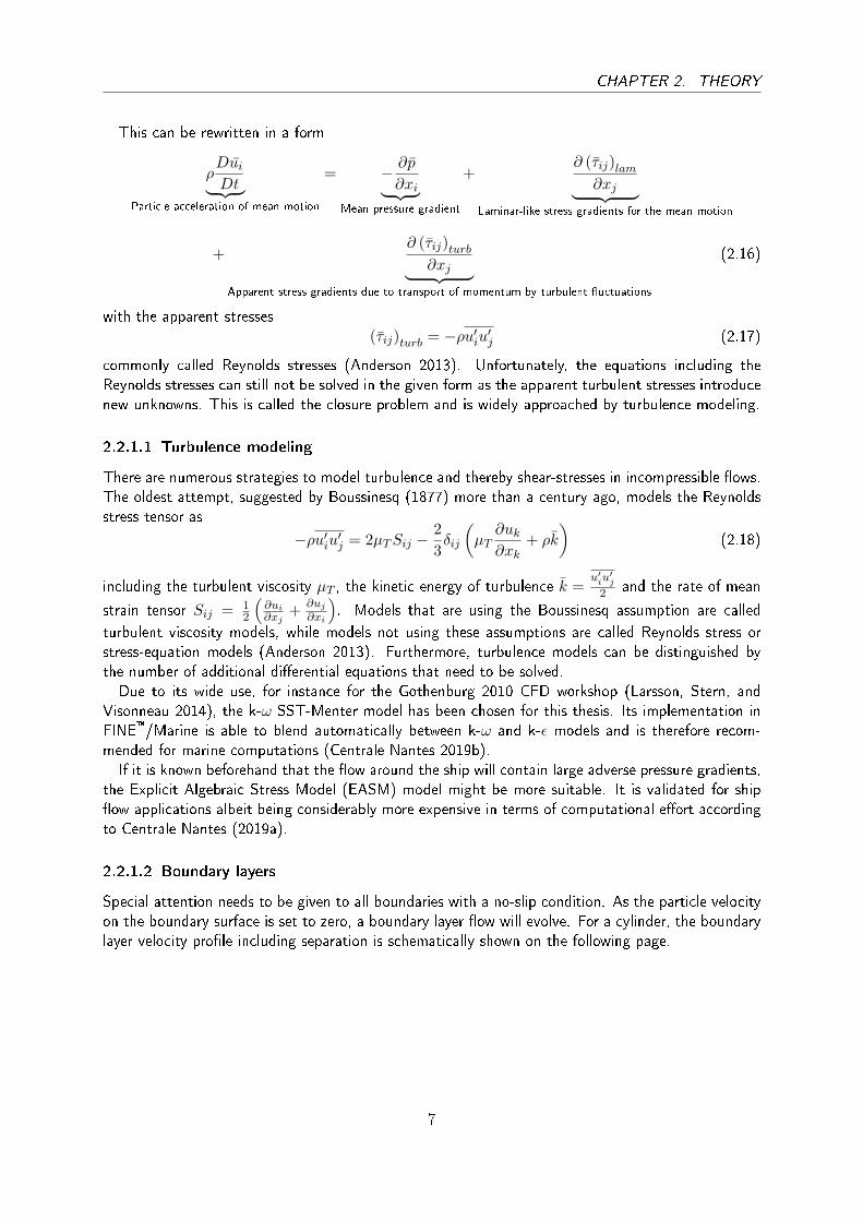
This can be rewritten in a form

ρDuiDt︸︷︷︸

Particle acceleration of mean motion

= − ∂p

∂xi︸︷︷︸Mean pressure gradient

+∂ (τij)lam∂xj︸︷︷︸

Laminar-like stress gradients for the mean motion

+∂ (τij)turb∂xj︸︷︷︸

Apparent stress gradients due to transport of momentum by turbulent �uctuations

(2.16)

with the apparent stresses(τij)turb = −ρu′iu′j (2.17)

commonly called Reynolds stresses (Anderson 2013). Unfortunately, the equations including theReynolds stresses can still not be solved in the given form as the apparent turbulent stresses introducenew unknowns. This is called the closure problem and is widely approached by turbulence modeling.

2.2.1.1 Turbulence modeling

There are numerous strategies to model turbulence and thereby shear-stresses in incompressible �ows.The oldest attempt, suggested by Boussinesq (1877) more than a century ago, models the Reynoldsstress tensor as

−ρu′iu′j = 2µTSij −2

3δij

(µT

∂uk∂xk

+ ρk

)(2.18)

including the turbulent viscosity µT , the kinetic energy of turbulence k =u′iu

′j

2 and the rate of mean

strain tensor Sij = 12

(∂ui∂xj

+∂uj∂xi

). Models that are using the Boussinesq assumption are called

turbulent viscosity models, while models not using these assumptions are called Reynolds stress orstress-equation models (Anderson 2013). Furthermore, turbulence models can be distinguished bythe number of additional di�erential equations that need to be solved.Due to its wide use, for instance for the Gothenburg 2010 CFD workshop (Larsson, Stern, and

Visonneau 2014), the k-ω SST-Menter model has been chosen for this thesis. Its implementation inFINE�/Marine is able to blend automatically between k-ω and k-ε models and is therefore recom-mended for marine computations (Centrale Nantes 2019b).If it is known beforehand that the �ow around the ship will contain large adverse pressure gradients,

the Explicit Algebraic Stress Model (EASM) model might be more suitable. It is validated for ship�ow applications albeit being considerably more expensive in terms of computational e�ort accordingto Centrale Nantes (2019a).

2.2.1.2 Boundary layers

Special attention needs to be given to all boundaries with a no-slip condition. As the particle velocityon the boundary surface is set to zero, a boundary layer �ow will evolve. For a cylinder, the boundarylayer velocity pro�le including separation is schematically shown on the following page.

7

CHAPTER 2. THEORY

Figure 2.3: Flow-around cylinder (from Vigsnes 2018)

As can be seen, the velocity pro�le contains high gradients in the direction normal to the wall. Inorder to capture these gradients properly, viscous layers need to be inserted into the initial mesh.To limit the number of inserted cells for the boundary layer, wall-functions are used within this

thesis. The non-dimensional size of the �rst cell in the boundary layer is estimated prior to thesimulation based on the formula

y+ = max

(30; min

(30 +

(Re− 106

)· 270

109; 300

))(2.19)

by FINE�/Marine (Centrale Nantes 2019b). Although the use of wall-functions adds another uncer-tainty to the simulation, this strategy is very useful and recommended by Centrale Nantes (2019b) tospeed up the computation. It decreases the number of cells signi�cantly compared to a mesh withoutwall-functions.

2.2.2 Euler method

By neglecting all shear stresses and thereby any turbulence in the �ow, the Euler equation can beused to solve the �ow problem. The set of di�erential equations can obtained from formula 2.10 bydropping all viscous terms and yields to

ρDV

Dt= ρf −∇p (2.20)

(Anderson 2013). The general Euler equation is not to be confused with potential �ow. As forpotential �ow, irrotational �ow is assumed which is generally not the case for the Euler equation.The implementation of Euler �ow in FINE�/Marine does not assume irrotational �ow. Hence, it

does not make use of the possible advantage - having analytical description of the �ow �eld - albeitneglecting viscous e�ects completely. Compared to dedicated potential �ow codes (as described insection 2.1.2.2), assuming rotational inviscid �ow does barely outweigh the additional computationale�ort.

8

CHAPTER 2. THEORY

2.2.3 Discretization of computational domain and free surface capturing

Generally, within CFD (excluding potential �ow), three approaches to discretization of the computa-tional domain exist (Bertram 2012b):

� Finite element methods (FEM)

� Finite di�erence methods (FDM)

� Finite volume methods (FVM)

Although FEM can be applied to �uid mechanics, it is rarely used in ship applications. FDM andFVM are the more common methods with comparable accuracy. Due to the fact, that FVM ensuresconservation of mass and momentum by design, this method is nowadays more popular than FDM.Within FINE�/Marine, the FVM in combination with the Volume of Fluid approach is used to

capture the free surface in multi-�uid �ows. That means that each cell is assigned a value between0 and 1, depending on the amount of water (or similar �uid) they contain. The free surface can thusbe reconstructed by tracking those cells with a value between 0 and 1.

9

3 Methodology and computational set-up

3.1 Methods investigated in this thesis

Although potential �ow and computational �uid dynamics (RANS/Euler) solvers have so far shownsimilar agreement with respect to determining the motions and also added wave resistance, only RANSsolvers are able to account accurately enough for viscous e�ects. These viscous e�ects can play animportant role, for example in the wake �ow for a propulsor, and hence are of great interest in earlydesign phases already. Being a promising engineering tool for the ship designer, the computational �owmethod is subject to investigations of this thesis. The application of CFD to seakeeping simulationsis investigated using FINE�/Marine�'s software package. Di�erent computational settings (�ow type,wave length, mesh re�nement etc., see section 3.4) are applied to a test vessel and thus, a best-practiceprocedure for the computational �ow method shall be established.

3.2 Model description

Due to its wide use for research purposes, the KVLCC2 vessel has been selected as a test case forthis study. Furthermore, the vessel has recently been tested in SSPA's towing tank as well as withSHIPFLOW® Motions inhouse CFD solver.Albeit vessel characteristics, such as added wave resistance coe�cient or heave RAO are usually

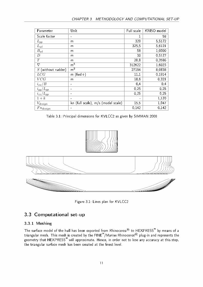
compared non-dimensionally, the vessel is used in model scale (KRISO model) within this study.This enables comparison of dimensional parameters with studies performed at Norwegian Universityof Science and Technology (NTNU, Vigsnes 2018) and SINTEF Ocean research institute (formerlyMarintek), where KRISO model scale (1:58) was tested (Guo, Steen, and Deng 2012).The principal dimensions of KVLCC2 in full and model scale as well as a lines plan are shown on

the next page.

10

CHAPTER 3. METHODOLOGY AND COMPUTATIONAL SET-UP

Parameter Unit Full scale KRISO model

Scale factor - 1 58

Lpp m 320 5,5172

Lwl m 325,5 5,6121

Bwl m 58 1,0000

D m 30 0,5172

T m 20,8 0,3586

∇ m3 312622 1,6023

S (without rudder) m2 27194 8,0838

LCG m (fwd+) 11,1 0,1914

V CG m 18,6 0,321

ixx/B - 0,4 0,4

iyy/Lpp - 0,25 0,25

izz/Lpp - 0,25 0,25

1 + k - - 1,170

Vdesign kn (full scale), m/s (model scale) 15,5 1,047

Fndesign - 0,142 0,142

Table 3.1: Principal dimensions for KVLCC2 as given by SIMMAN 2008

Figure 3.1: Lines plan for KVLCC2

3.3 Computational set-up

3.3.1 Meshing

The surface model of the hull has been exported from Rhinoceros® to HEXPRESS� by means of atriangular mesh. This mesh is created by the FINE�/Marine Rhinoceros® plug-in and represents thegeometry that HEXPRESS� will approximate. Hence, in order not to lose any accuracy at this step,the triangular surface mesh has been created at the �nest level.

11


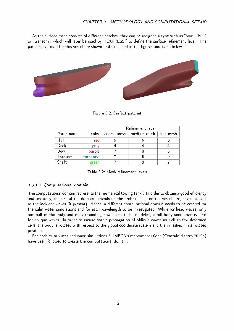
As the surface mesh consists of di�erent patches, they can be assigned a type such as �bow�, �hull�or �transom�, which will later be used by HEXPRESS� to de�ne the surface re�nement level. Thepatch types used for this vessel are shown and explained in the �gures and table below.

Figure 3.2: Surface patches

Re�nement level

Patch name color coarse mesh medium mesh �ne mesh

Hull red 5 6 6

Deck gray 4 4 4

Bow purple 7 8 8

Transom turquoise 7 8 9

Shaft green 7 8 9

Table 3.2: Mesh re�nement levels

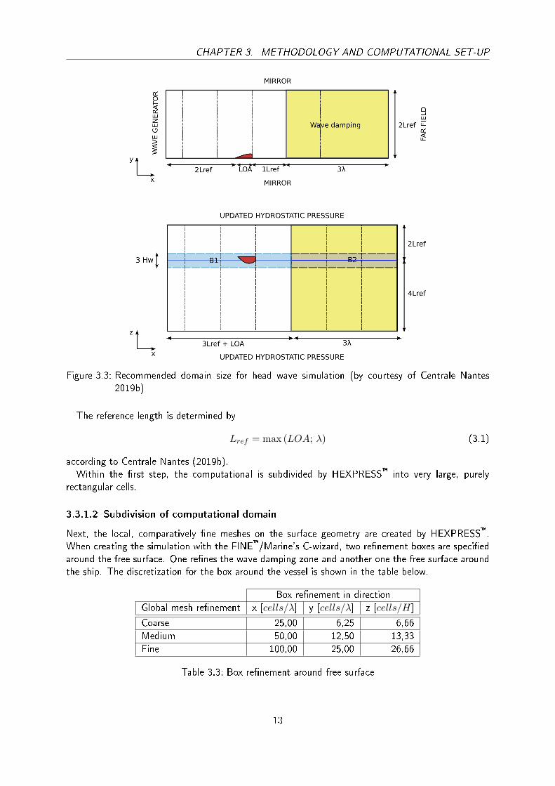
3.3.1.1 Computational domain

The computational domain represents the �numerical towing tank�. In order to obtain a good e�ciencyand accuracy, the size of the domain depends on the problem, i.e. on the vessel size, speed as wellas the incident waves (if present). Hence, a di�erent computational domain needs to be created forthe calm water simulations and for each wavelength to be investigated. While for head waves, onlyone half of the body and its surrounding �ow needs to be modeled, a full body simulation is usedfor oblique waves. In order to ensure stable propagation of oblique waves as well as few deformedcells, the body is rotated with respect to the global coordinate system and then meshed in its rotatedposition.For both calm water and wave simulations NUMECA's recommendations (Centrale Nantes 2019b)

have been followed to create the computational domain.

12


Figure 3.3: Recommended domain size for head wave simulation (by courtesy of Centrale Nantes2019b)

The reference length is determined by

Lref = max (LOA; λ) (3.1)

according to Centrale Nantes (2019b).Within the �rst step, the computational is subdivided by HEXPRESS� into very large, purely

rectangular cells.

3.3.1.2 Subdivision of computational domain

Next, the local, comparatively �ne meshes on the surface geometry are created by HEXPRESS�.When creating the simulation with the FINE�/Marine's C-wizard, two re�nement boxes are speci�edaround the free surface. One re�nes the wave damping zone and another one the free surface aroundthe ship. The discretization for the box around the vessel is shown in the table below.

Box re�nement in direction

Global mesh re�nement x [cells/λ] y [cells/λ] z [cells/H]

Coarse 25,00 6,25 6,66

Medium 50,00 12,50 13,33

Fine 100,00 25,00 26,66

Table 3.3: Box re�nement around free surface

13


It should be noted, that the coarse mesh re�nement is not completely in line with InternationalTowing Tank Conference (2011a), which recommends at least 40 cells in x-direction for regular waves.For irregular waves however, no less than 20 grid points are recommended which is satis�ed here.The minimum re�nement in the vertical direction agrees with International Towing Tank Conference(2011a), as the re�nement box extends about 3 wave heights around the free surface correspondingto the recommended minimum 20 grid points.

3.3.1.3 Viscous layers

For all viscous simulations, additional viscous layer cells are created around all surfaces with a 'no-slip'condition, i.e. the hull surfaces except for the deck. HEXPRESS� automatically takes care of the�rst cell layer thickness as explained in section 2.2.1.2.

3.3.2 Multi-�uid model

For this multi-�uid simulation, water with a kinematic viscosity of η = 1.1386 · 10−6[m2/s

]and a

density of ρwater = 999, 1026[kg/m3

]is used. This corresponds to fresh water at a temperature

of 15 °C. The air is modeled by a �uid with dynamic viscosity of µ = 1, 85 · 10−5 [Pa · s] and a airdensity of ρair = 1, 2

[kg/m3

]. Furthermore, the gravity is set to g = 9, 81

[m/s2

].

3.3.2.1 Flow model

Both viscous and inviscid �ow are investigated in this study. As explained in section 2.2.1.1, viscousturbulent �ow is modeled by k-ω SST-Menter model and inviscid simulations with Euler type of �ow.

3.3.3 Boundary conditions

Due to the density of air, the shear stresses on the deck can be neglected if no water-on-deck conditionoccurs. Thus, the boundary condition on the deck is always set to 'slip'.For the viscous simulations, wall-functions are used in combination with the 'no-slip' boundary

condition on the remaining parts of the hull. For inviscid simulations, a simple 'no-slip' condition isused all over the hull.The domain boundaries are modeled as a far �eld condition (outlet behind the wave damping zone),

a prescribed pressure condition (for the bottom and top of the domain, incl. updated hydrostaticpressure) and mirror conditions for both boundaries in the xz-plane.

3.3.3.1 Wave generation

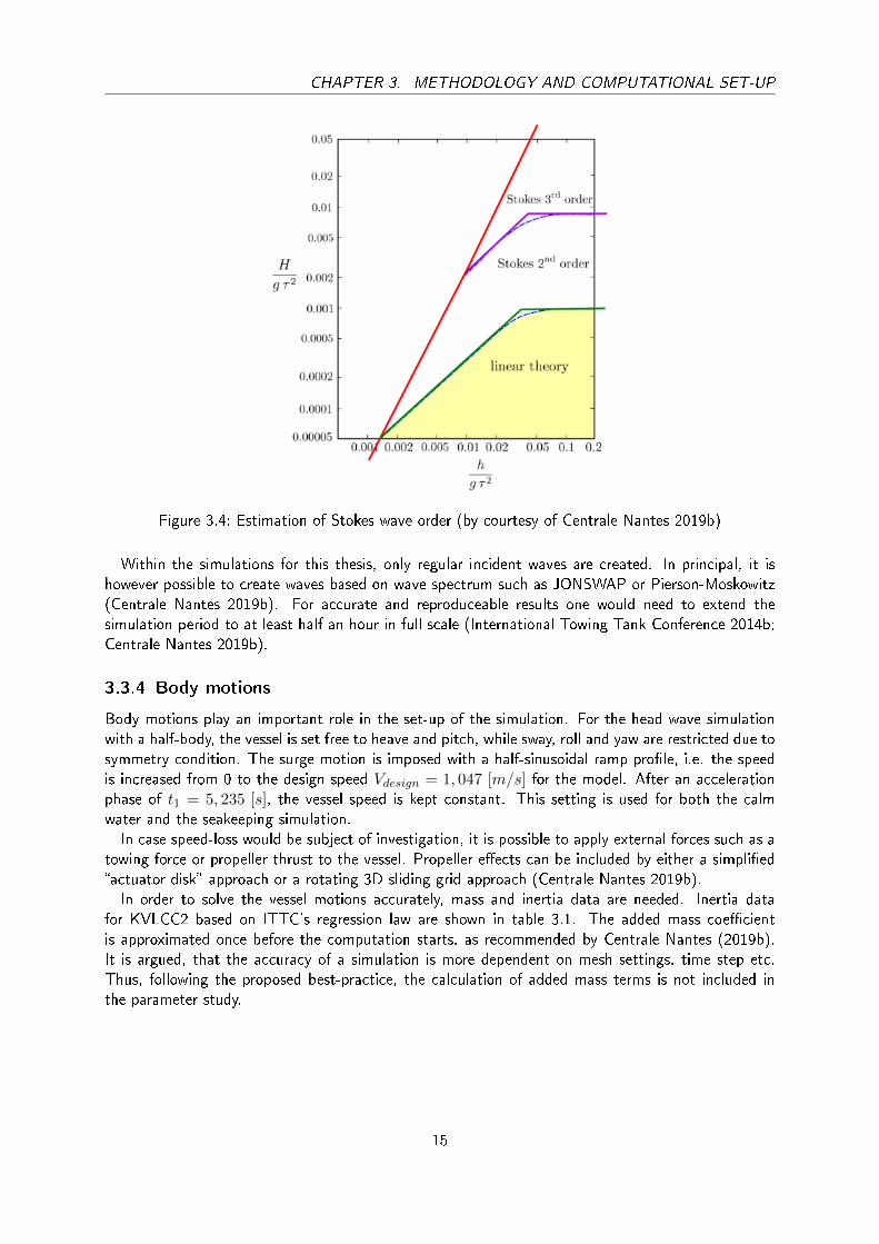
Furthermore, the upstream inlet boundary contains a so-called 'boundary wave creator'. Accordingto Centrale Nantes (2019b), the boundary wave creator is to be preferred over an internal wavegenerator, when the ship is moving forward with a certain speed. When specifying forward speed inFINE�/Marine's C-wizard, the boundary wave creator is used by default.Stokes waves from 1st to 3rd order can be applied and the estimation of the wave order is auto-

matically performed according to the following graph:

14


Figure 3.4: Estimation of Stokes wave order (by courtesy of Centrale Nantes 2019b)

Within the simulations for this thesis, only regular incident waves are created. In principal, it ishowever possible to create waves based on wave spectrum such as JONSWAP or Pierson-Moskowitz(Centrale Nantes 2019b). For accurate and reproduceable results one would need to extend thesimulation period to at least half an hour in full scale (International Towing Tank Conference 2014b;Centrale Nantes 2019b).

3.3.4 Body motions

Body motions play an important role in the set-up of the simulation. For the head wave simulationwith a half-body, the vessel is set free to heave and pitch, while sway, roll and yaw are restricted due tosymmetry condition. The surge motion is imposed with a half-sinusoidal ramp pro�le, i.e. the speedis increased from 0 to the design speed Vdesign = 1, 047 [m/s] for the model. After an accelerationphase of t1 = 5, 235 [s], the vessel speed is kept constant. This setting is used for both the calmwater and the seakeeping simulation.In case speed-loss would be subject of investigation, it is possible to apply external forces such as a

towing force or propeller thrust to the vessel. Propeller e�ects can be included by either a simpli�ed�actuator disk� approach or a rotating 3D sliding grid approach (Centrale Nantes 2019b).In order to solve the vessel motions accurately, mass and inertia data are needed. Inertia data

for KVLCC2 based on ITTC's regression law are shown in table 3.1. The added mass coe�cientis approximated once before the computation starts, as recommended by Centrale Nantes (2019b).It is argued, that the accuracy of a simulation is more dependent on mesh settings, time step etc.Thus, following the proposed best-practice, the calculation of added mass terms is not included inthe parameter study.

15


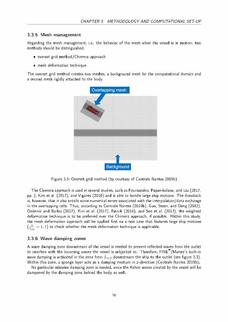
3.3.5 Mesh management

Regarding the mesh management, i.e. the behavior of the mesh when the vessel is in motion, twomethods should be distinguished:

� overset grid method/Chimera approach

� mesh deformation technique

The overset grid method creates two meshes, a background mesh for the computational domain anda second mesh rigidly attached to the body.

Figure 3.5: Overset grid method (by courtesy of Centrale Nantes 2019b)

The Chimera approach is used in several studies, such as Fournarakis, Papanikolaou, and Liu (2017,pp. ), Kim et al. (2017), and Vigsnes (2018) and is able to handle large ship motions. The drawbackis, however, that it also entails some numerical errors associated with the interpolation/data exchangein the overlapping cells. Thus, according to Centrale Nantes (2019b), Guo, Steen, and Deng (2012),Ozdemir and Barlas (2017), Kim et al. (2017), Rørvik (2016), and Seo et al. (2013), the weighteddeformation technique is to be preferred over the Chimera approach, if possible. Within this study,the mesh deformation approach will be applied �rst on a test case that features large ship motions( λLpp

= 1, 1) to check whether the mesh deformation technique is applicable.

3.3.6 Wave damping zones

A wave damping zone downstream of the vessel is needed to prevent re�ected waves from the outletto interfere with the incoming waves the vessel is subjected to. Therefore, FINE�/Marine's built-inwave damping is activated in the zone from Lref downstream the ship to the outlet (see �gure 3.3).Within this zone, a sponge layer acts as a damping medium in z-direction (Centrale Nantes 2019b).No particular sidewise damping zone is needed, since the Kelvin waves created by the vessel will be

dampened by the damping zone behind the body as well.

16


3.3.7 Time discretization and computational control

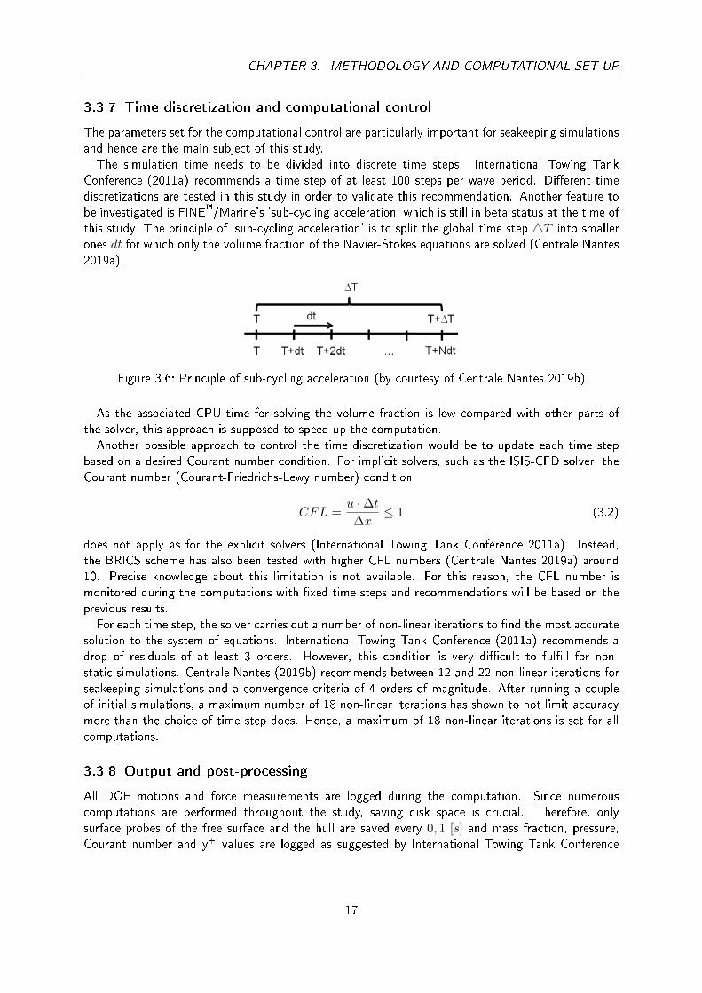
The parameters set for the computational control are particularly important for seakeeping simulationsand hence are the main subject of this study.The simulation time needs to be divided into discrete time steps. International Towing Tank

Conference (2011a) recommends a time step of at least 100 steps per wave period. Di�erent timediscretizations are tested in this study in order to validate this recommendation. Another feature tobe investigated is FINE�/Marine's 'sub-cycling acceleration' which is still in beta status at the time ofthis study. The principle of 'sub-cycling acceleration' is to split the global time step 4T into smallerones dt for which only the volume fraction of the Navier-Stokes equations are solved (Centrale Nantes2019a).

Figure 3.6: Principle of sub-cycling acceleration (by courtesy of Centrale Nantes 2019b)

As the associated CPU time for solving the volume fraction is low compared with other parts ofthe solver, this approach is supposed to speed up the computation.Another possible approach to control the time discretization would be to update each time step

based on a desired Courant number condition. For implicit solvers, such as the ISIS-CFD solver, theCourant number (Courant-Friedrichs-Lewy number) condition

CFL =u ·∆t∆x

≤ 1 (3.2)

does not apply as for the explicit solvers (International Towing Tank Conference 2011a). Instead,the BRICS scheme has also been tested with higher CFL numbers (Centrale Nantes 2019a) around10. Precise knowledge about this limitation is not available. For this reason, the CFL number ismonitored during the computations with �xed time steps and recommendations will be based on theprevious results.For each time step, the solver carries out a number of non-linear iterations to �nd the most accurate

solution to the system of equations. International Towing Tank Conference (2011a) recommends adrop of residuals of at least 3 orders. However, this condition is very di�cult to ful�ll for non-static simulations. Centrale Nantes (2019b) recommends between 12 and 22 non-linear iterations forseakeeping simulations and a convergence criteria of 4 orders of magnitude. After running a coupleof initial simulations, a maximum number of 18 non-linear iterations has shown to not limit accuracymore than the choice of time step does. Hence, a maximum of 18 non-linear iterations is set for allcomputations.

3.3.8 Output and post-processing

All DOF motions and force measurements are logged during the computation. Since numerouscomputations are performed throughout the study, saving disk space is crucial. Therefore, onlysurface probes of the free surface and the hull are saved every 0, 1 [s] and mass fraction, pressure,Courant number and y+ values are logged as suggested by International Towing Tank Conference

17


(2011a). Additionally, wave probes are created at di�erent locations in the domain to verify the waveheight.

3.3.8.1 Post-processing of calm water simulations

For both calm water and seakeeping simulations a separate post-processing script has been written inMATLAB (see appendix pages a and c respectively). Regarding the calm water simulation, the vesselresistance, heave and pitch are processed by means of exponential smoothing to improve stabilityof the measurements. As the physically most accurate solution can be expected at the end of thecomputation, the smoothing works backwards rather than traditionally from the beginning. Aftersmoothing the data, the average over the last 30% of the time is computed.

0 5 10 15 20 25 30 35 40 45

time [s]

-50

-45

-40

-35

-30

-25

-20

-15

-10

-5

0

Re

sis

tan

ce

[N

]

Computed Resistance

Smoothed Resistance

Average Resistance

Figure 3.7: Exponential smoothing of calm water resistance, shown here for �ne mesh RANS simula-tion

3.3.8.2 Post-processing of seakeeping simulation

While for the calm water resistance computations, post-processing of the logged data is straight-forward, the seakeeping simulation requires a somewhat di�erent approach. As proposed by theGothenburg 2010 CFD workshop (Larsson, Stern, and Visonneau 2014), a Fourier series is used toanalyze the variables resistance, heave and pitch. For each parameter (resistance, heave, pitch etc.),the Fourier series looks as follows:

P (t) =P0

2+

N∑n=1

Pn cos (2πfet+ γI) (3.3)

18


an =2

T

T

0

P (t) cos (2πfet) dt (3.4)

bn =2

T

T

0

P (t) sin (2πfet) dt (3.5)

Pn =√a2n + b2n (3.6)

In MATLAB this could easily be implemented with the discrete Fourier transformation function '�t'(fast Fourier transformation). However, this function requires a uniform sampling rate, i.e. the timestep needs to be constant. Due to the envisaged Courant-based time step adaption (see section3.3.7), this cannot be guaranteed throughout the entire study. For this reason, the Fourier series iscomputed by the built-in �t function. The �t function approximates an 8th-order Fourier function toa given data set. International Towing Tank Conference (2014b) recommends using at least 10 waveencounters. Hence, the last 10 wave encounters are analyzed by means of the Fourier transformation:

-20 -15 -10 -5 0 5 10

time [s]

-0.2

-0.1

0

0.1

0.2

0.3

0.4

0.5

Pitch a

ngle

[°]

Computed time series

Fourier function

cut time

Figure 3.8: Fourier analysis of pitch motion, exemplary shown for a coarse mesh and λ/Lpp = 0, 6

19


In order to extract the 1st harmonic of the Fourier series, the coe�cients an and bn belonging tothe encounter frequency can be read out.In addition to the Fourier analysis, the Courant number is monitored throughout the simulation.

Therefore, the measure 'Courant95' is established which depicts the Courant number, that is higherthan 95% of the recorded values as an envelope for each simulation.

-25 -20 -15 -10 -5 0 5 10 15

time [s]

0

0.5

1

1.5

2

2.5

3

3.5

4

4.5

Coura

nt n

um

ber


Courant number 95%

cut time

Figure 3.9: Measure 'Courant95', exemplary shown for a coarse mesh and λ/Lpp = 1, 1

3.3.8.3 Subtraction of calm water resistance from total resistance

To obtain the mean added resistance in waves, the calm water resistance RT,calm needs to be sub-tracted from the mean resistance in waves RT,waves = P0

2 . As di�erent domains are used for the calmwater resistance simulation and for each wave simulation, the corresponding coarse, medium and �nemesh simulations are linked accordingly. Thus, it is always the coarse mesh calm water resistance thatis subtracted from the coarse mesh resistance in waves. The same principle applies to the inviscidsimulations, where the di�erence between a coarse inviscid calm water simulation and a coarse Eulerwave simulation is taken.Although this procedure is not based on the most accurate result (being from a �ne mesh simulation

or EFD), it represents a very practical approach to a new vessel design, that has not been subject toresearch studies over several years.

3.4 Parameters to be investigated

Di�erent computational set-ups with respect to the following parameters will be investigated:

� �ow type: Euler type of �ow, viscous �ow with (SST-Menter turbulence model)

20


� wave length: λLpp

= [0, 6; 1, 1; 1, 6]

� wave encountering angle: 180◦ and 160◦

� mesh re�nement: coarse, medium and �ne mesh

� time discretization: �xed time step from 50 to 400 time steps per wave period; Courant-adaptedtime step; sub-cycling acceleration

The number of parameters implies that not all possible combinations could have been investigated. Inorder to keep the computational time low, the focus has been on the most promising con�gurationsto produce conclusive results.

3.5 Computational resources

During the time of the thesis, two academic licenses for the NUMECA's FINE�/Marine softwarepackage (version 7.2.1) with ISIS-CFD solver have been available. While one of these licenses wasrestricted to a quad-core laptop, the other one could be used for computations on SSPA's morepowerful network machines. Due to changing availability of SSPA's machines for the project, not allof the computations could be performed on the most powerful machine in the network. This makes itsomewhat di�cult to compare absolute values of elapsed computational time. However, this was thebest way to perform as many simulations as possible. The appendix (page i and following) containsa list of machines used for computations and their respective technical data .When assessing the suitability of a computer to a certain simulation, one should keep two principles

in mind:

� Larger meshes generally run faster on several cores, as they can work in parallel.

� Increased GHz will speed up the computation of following time steps

With respect to parallel computing, the gain in speed however diminishes with growing number ofprocessors. This is due to the fact, that the cells assigned to a processor communicate by means of'overlapping ghost cells' (Centrale Nantes 2019b). If relatively few cells are assigned to numerousprocessors, this communication takes up a large portion of time and the ratio ghost cells/total amountof cells increases.

21

4 Results and discussion

4.1 Wave study

As point probes have been speci�ed within the computational domain, the wave height at discretepoints can measured. The post-processing of the wave probes (MATLAB script, appendix page gand following) is done similarly to the post-processing of motions and resistance in section 3.3.8.2,albeit for the waves only a 2nd order Fourier function is taken as the waves are created by 2nd orderNavier-Stokes boundary wave creator.

22

CHAPTER 4. RESULTS AND DISCUSSION

0 5 10 15 20 25 30 35 40 45

time [s]

0.31

0.32

0.33

0.34

0.35

0.36

0.37

0.38

0.39

0.4

0.41

H [m

]

Time-history

-25 -20 -15 -10 -5 0 5 10 15 20

time [s]

0.3

0.32

0.34

0.36

0.38

0.4

0.42

Wave e

levation [m

]


Fourier function

cut time

Figure 4.1: Recorded (top) and approximated time series (bottom) of wave probe no. 4, coarse mesh,λLpp

= 1, 6 and 200 time steps per wave period

The results of the wave study are exemplary presented for the coarse mesh and long waves ( λLpp

=

1, 6) and various time steps. The nominal incident wave height is set to H = 0, 0883 [m] for theseconditions.

23


Time steps per wave period50 100 150 200 400

Probe no. x [m] y [m] H [m] H [m] H [m] H [m] H [m]

1 5,5712 (Lpp) 0 0,4275 0,4076 0,4065 0,4072 0,4076

2 5,5712 (Lpp) 1 0,0947 0,1041 0,1049 0,1042 0,1032

3 5,5712 (Lpp) 5 0,0719 0,0831 0,0856 0,0863 0,0866

4 5,5712 (Lpp) 10 0,0731 0,0840 0,0864 0,0870 0,0873

5 12 0 0,0789 0,0856 0,0869 0,0875 0,0879

6 23,3117 (inlet BC) 0 0,0950 0,0962 0,0964 0,0965 0,0966

7 23,3117 (inlet BC) 1 0,0950 0,0962 0,0964 0,0965 0,0966

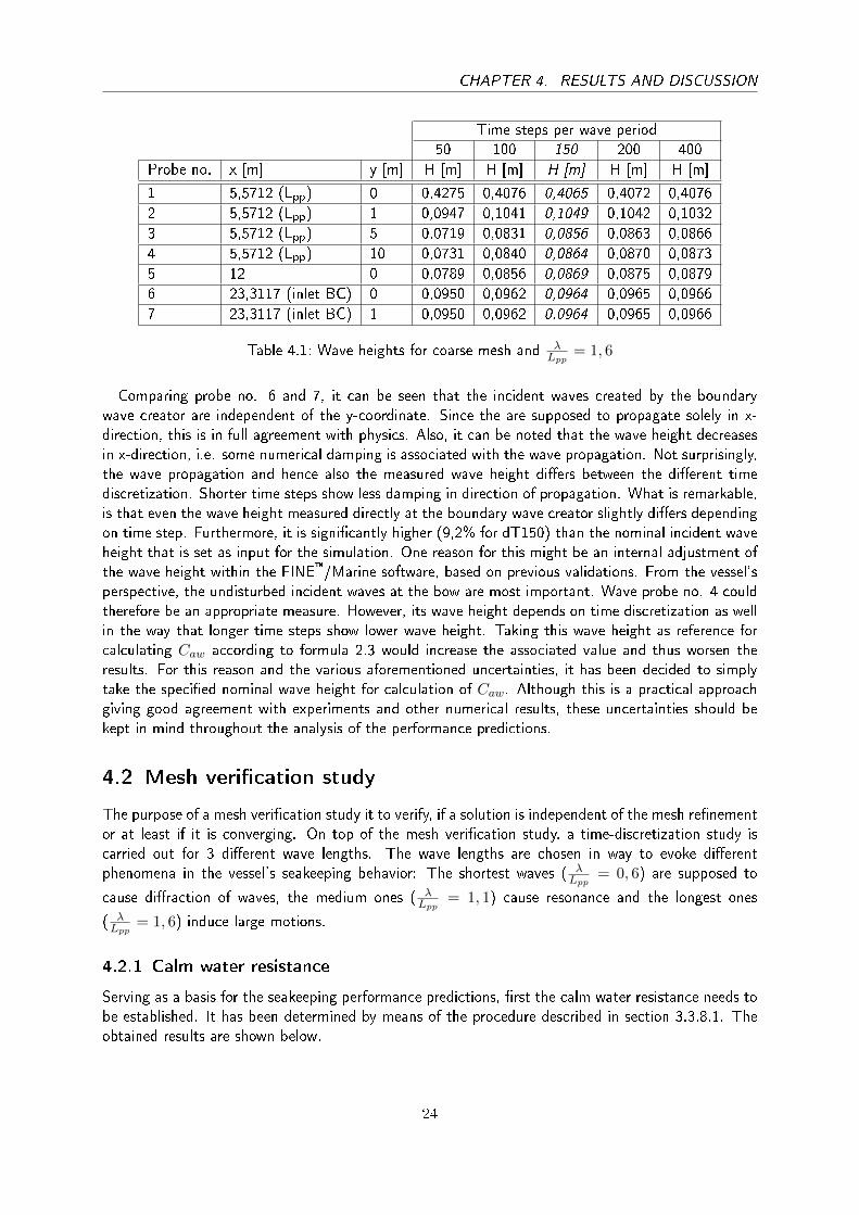
Table 4.1: Wave heights for coarse mesh and λLpp

= 1, 6

Comparing probe no. 6 and 7, it can be seen that the incident waves created by the boundarywave creator are independent of the y-coordinate. Since the are supposed to propagate solely in x-direction, this is in full agreement with physics. Also, it can be noted that the wave height decreasesin x-direction, i.e. some numerical damping is associated with the wave propagation. Not surprisingly,the wave propagation and hence also the measured wave height di�ers between the di�erent timediscretization. Shorter time steps show less damping in direction of propagation. What is remarkable,is that even the wave height measured directly at the boundary wave creator slightly di�ers dependingon time step. Furthermore, it is signi�cantly higher (9,2% for dT150) than the nominal incident waveheight that is set as input for the simulation. One reason for this might be an internal adjustment ofthe wave height within the FINE�/Marine software, based on previous validations. From the vessel'sperspective, the undisturbed incident waves at the bow are most important. Wave probe no. 4 couldtherefore be an appropriate measure. However, its wave height depends on time discretization as wellin the way that longer time steps show lower wave height. Taking this wave height as reference forcalculating Caw according to formula 2.3 would increase the associated value and thus worsen theresults. For this reason and the various aforementioned uncertainties, it has been decided to simplytake the speci�ed nominal wave height for calculation of Caw. Although this is a practical approachgiving good agreement with experiments and other numerical results, these uncertainties should bekept in mind throughout the analysis of the performance predictions.

4.2 Mesh veri�cation study

The purpose of a mesh veri�cation study it to verify, if a solution is independent of the mesh re�nementor at least if it is converging. On top of the mesh veri�cation study, a time-discretization study iscarried out for 3 di�erent wave lengths. The wave lengths are chosen in way to evoke di�erentphenomena in the vessel's seakeeping behavior: The shortest waves ( λ

Lpp= 0, 6) are supposed to

cause di�raction of waves, the medium ones ( λLpp

= 1, 1) cause resonance and the longest ones

( λLpp

= 1, 6) induce large motions.

4.2.1 Calm water resistance

Serving as a basis for the seakeeping performance predictions, �rst the calm water resistance needs tobe established. It has been determined by means of the procedure described in section 3.3.8.1. Theobtained results are shown below.

24


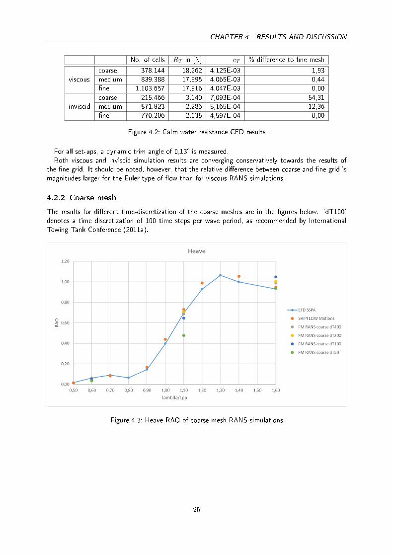
No. of cells RT in [N] cT % di�erence to �ne mesh

viscouscoarse 378.144 18,262 4,125E-03 1,93medium 839.388 17,995 4,065E-03 0,44�ne 1.103.657 17,916 4,047E-03 0,00

inviscidcoarse 215.466 3,140 7,093E-04 54,31medium 571.823 2,286 5,165E-04 12,36�ne 770.206 2,035 4,597E-04 0,00

Figure 4.2: Calm water resistance CFD results

For all set-ups, a dynamic trim angle of 0,13° is measured.Both viscous and inviscid simulation results are converging conservatively towards the results of

the �ne grid. It should be noted, however, that the relative di�erence between coarse and �ne grid ismagnitudes larger for the Euler type of �ow than for viscous RANS simulations.

4.2.2 Coarse mesh

The results for di�erent time-discretization of the coarse meshes are in the �gures below. 'dT100'denotes a time discretization of 100 time steps per wave period, as recommended by InternationalTowing Tank Conference (2011a).

Figure 4.3: Heave RAO of coarse mesh RANS simulations

25


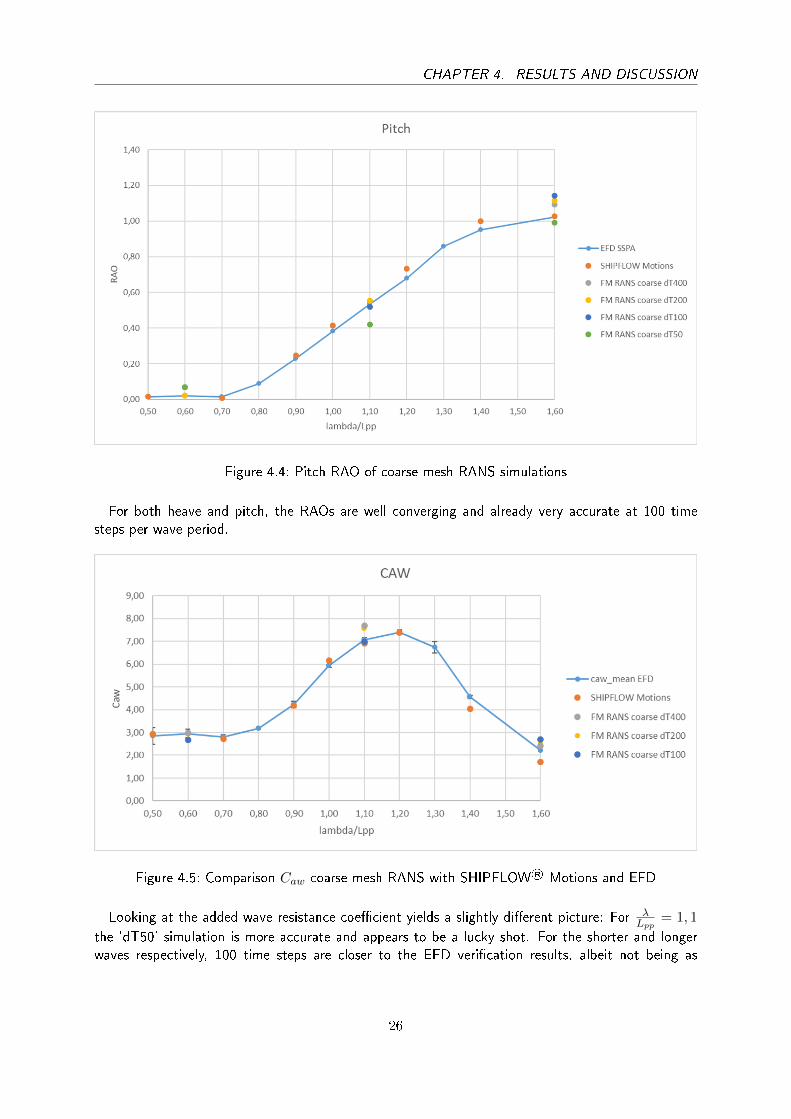
Figure 4.4: Pitch RAO of coarse mesh RANS simulations

For both heave and pitch, the RAOs are well converging and already very accurate at 100 timesteps per wave period.

Figure 4.5: Comparison Caw coarse mesh RANS with SHIPFLOW® Motions and EFD

Looking at the added wave resistance coe�cient yields a slightly di�erent picture: For λLpp

= 1, 1

the 'dT50' simulation is more accurate and appears to be a lucky shot. For the shorter and longerwaves respectively, 100 time steps are closer to the EFD veri�cation results, albeit not being as

26


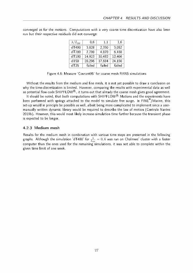
converged as for the motions. Computations with a very coarse time discretization have also beenrun but their respective residuals did not converge:

λ/Lpp 0,6 1,1 1,6

dT400 3,828 2,330 3,052

dT200 7,780 4,870 6,188

dT100 14,923 10,492 12,466

dT50 28,296 17,684 24,150

dT25 failed failed failed

Figure 4.6: Measure 'Courant95' for coarse mesh RANS simulations

Without the results from the medium and �ne mesh, it is not yet possible to draw a conclusion onwhy the time-discretization is limited. However, comparing the results with experimental data as wellas potential �ow code SHIPFLOW®, it turns out that already the coarse mesh gives good agreement.It should be noted, that both computations with SHIPFLOW® Motions and the experiments have

been performed with springs attached to the model to simulate free surge. In FINE�/Marine, thisset-up would in principle be possible as well, albeit being more complicated to implement since a user-manually written dynamic library would be required to describe the law of motion (Centrale Nantes2019b). However, this would most likely increase simulation time further because the transient phaseis expected to be longer.

4.2.3 Medium mesh

Results for the medium mesh in combination with various time steps are presented in the followinggraphs. Although the simulation 'dT400' for λ

Lpp= 0, 6 was run on Chalmers' cluster with a faster

computer than the ones used for the remaining simulations, it was not able to complete within thegiven time limit of one week.

27


Figure 4.7: Heave RAO of medium mesh RANS simulations

Figure 4.8: Pitch RAO of medium mesh RANS simulations

Similarly to the coarse mesh, sub-cycling acceleration did not help to stabilize the computationas the residuals did not converge. The respective results are therefore incorrect and left out in thefollowing plot:

28


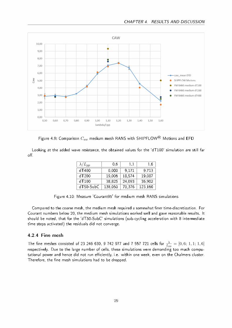
Figure 4.9: Comparison Caw medium mesh RANS with SHIPFLOW® Motions and EFD

Looking at the added wave resistance, the obtained values for the 'dT100' simulation are still faro�.

λ/Lpp 0,6 1,1 1,6

dT400 0,000 9,171 9,713

dT200 19,006 18,574 19,087

dT100 38,825 24,093 36,902

dT50-SubC 138,050 70,376 123,160

Figure 4.10: Measure 'Courant95' for medium mesh RANS simulations

Compared to the coarse mesh, the medium mesh required a somewhat �ner time-discretization. ForCourant numbers below 20, the medium mesh simulations worked well and gave reasonable results. Itshould be noted, that for the 'dT50-SubC' simulations (sub-cycling acceleration with 8 intermediatetime steps activated) the residuals did not converge.

4.2.4 Fine mesh

The �ne meshes consisted of 23 246 630, 9 742 977 and 7 557 721 cells for λLpp

= [0, 6; 1, 1; 1, 6]

respectively. Due to the large number of cells, these simulations were demanding too much compu-tational power and hence did not run e�ciently, i.e. within one week, even on the Chalmers cluster.Therefore, the �ne mesh simulations had to be dropped.

29


4.3 Inviscid �ow simulation

As inviscid �ow neglects viscous e�ects, the additional cells for re�nement of the viscous layers aroundthe hull can be omitted. Thus, savings between 26% and 41% in mesh count have been achieved.Additionally, less equations need to be solved for each cell giving a potential advantage for the inviscidEuler �ow simulations.The motion RAOs can be determined with su�ucient accuracy in inviscid �ow:

Figure 4.11: Heave RAO of coarse mesh Euler simulations

30


Figure 4.12: Pitch RAO of coarse mesh Euler simulations

However, the added wave resistance is converging towards a too high value for the medium wavelength λ

Lpp= 1, 1 at resonance frequency.

Figure 4.13: Caw RAO of coarse mesh Euler simulations

It turns out that the Euler �ow computations required a �ner time-discretization (dT200) in order

31


to converge properly. This outweighs the potential gain in speed to a certain extend.Furthermore, for the shortest waves, the residuals of the computation did not consistently converge

towards zero:

Figure 4.14: Residuals of inviscid computation for λLpp

= 0,6 and 200 time steps per wave period

For these reasons, the Euler �ow computations cannot be seen as robust and reliable. Eventually,they neither outperform the RANS simulations in terms of computational speed nor in accuracy.

4.4 Courant-adapted time step

Based on the previous results from the coarse and medium mesh computations, a Courant numberlimit of 15 has been chosen in order to determine the time step. In order to emphasize the Courant-adapted time step feature, a very coarse global resolution of only 50 time steps per wave period hasbeen chosen.

32


Figure 4.15: Heave RAO of Courant-adapted time step simulation

Figure 4.16: Pitch RAO of Courant-adapted time step simulation

33


Figure 4.17: Caw RAO of Courant-adapted time step simulation

The results indicate, that the Courant-based time step is not a reliable way to speed up or re�ne acomputation. The Courant-based time law hardly improves the accuracy compared to a global timestep of 50, while still not giving good results.

4.5 Final choice of time step

The previous investigations have shown, that a coarse mesh in combination with 100 to 200 timesteps per wave period and RANS viscous equations can give accurate results. As computational timeapproximately doubles with an increase from 100 to 200 time steps per wave period, another set-upwith 150 time steps is tested in order to bridge the gap.The results in terms of motions and added wave resistance are presented on the next pages.

34


Figure 4.18: Heave RAO of the coarse mesh simulations with optimum time step

Figure 4.19: Pitch RAO of the coarse mesh simulations with optimum time step

35


Figure 4.20: Caw RAO of the coarse mesh simulations with optimum time step

As can be seen for λLpp

= 1, 1 for example, 150 time steps per wave period yields better converged

results than those computations with 100 time steps, yet still saves 25% of time compared to 200while maintaining similar accuracy.

4.6 Oblique waves

Although data for oblique wave conditions is scarce, some CFD results from NTNU (Vigsnes 2018) foroblique wave conditions exist. Hence, the same wave conditions have been applied and additionally,simulations for the three previously used conditions are carried out.

Test case λLpp

H [m] Hλ [%] T [s] λ [m] Wave encounter angle [°]

NTNU (Vigsnes 2018) 0,9176 0,1489 2,94 1,8007 5,0626 160

This thesis/SSPA 0,6 0,0662 2,00 1,4561 3,3103 160

This thesis/SSPA 1,1 0,0607 1,00 1,9716 6,0690 160

This thesis/SSPA 1,6 0,0883 1,00 2,3778 8,8276 160

Table 4.2: Test cases for oblique wave conditions

As for the oblique wave conditions, the best-practice determined from head wave simulations isapplied. That is 150 time steps per wave period for time discretization and a coarse mesh usingSST-Menter turbulence model.Unfortunately, modeling free yaw motion with a rotational spring did not work, since the spring

moment is calculated based on the actual Cardan angle of the vessel and would thus be in equilibriumfor 0° heading angle. As further workarounds, such as rotating the vessel's inertia moments failed as

36


well, the simulation had to be performed with a �xed yaw angle. Unlike for head waves, the vessel isset free to roll now.

4.6.1 Comparison with CFD calculations of a thesis study at NTNU

Within the same wave conditions, the results in terms of mean total resistance between this thesisand Vigsnes (2018) only di�er by 1,27%. This can be seen as very good agreement, taking intoaccount the coarse mesh for this simulation as well as unknown water properties for Vigsnes (2018)simulation.

Test case RT,waves [N] 1st harmonic Heave [m] 1st harmonic roll [°] 1st harmonic pitch [°]

NTNU (Vigsnes 2018) 67,64 0,030 0,080 2,339

This thesis 68,50 0,021 0,042 1,745

E%D +1,27% -31,33% -48,13% -25,40%

Figure 4.21: Comparison seakeeping results in oblique waves

Looking at the 1st harmonics of motions, the scatter is much larger. One reason, amongst others,could be sought in a di�erent post-processing procedure:

-30 -25 -20 -15 -10 -5 0 5 10 15

time [s]

-0.3

-0.25

-0.2

-0.15

-0.1

-0.05

0

0.05

0.1

Roll

angle

[°]


Fourier function

cut time

Figure 4.22: Recorded (blue) and approximated (red) time-series of roll motion for oblique wave con-ditions

As can be seen from the above plot, the roll motion is composed of di�erent harmonics withnon-zero amplitudes. That being said, the results depend a lot on the implemented post-processingprocedure, i.e. how many waves are taken into account or the way Fourier transformation is used.

37


4.6.2 Comparison with head waves

In addition to the oblique wave conditions used by Vigsnes (2018), the previously used head waveshave been applied with a 160° heading angle, too. The resulting added wave resistance RAOs -compared to head waves - are shown in the graph below.

Figure 4.23: Caw RAO comparison between head waves and oblique waves

It is remarkable, that the added resistance due to incident waves increases for 160° wave encounterangle. This is well in line with the �ndings from Vigsnes (2018) and Bertram and Courser (and 2014),who estimate about 10% higher added resistance in oblique waves as a rule of thumb. In fact, for theshortest set of applied oblique waves, the increase is as high as 14% here.

38


λLpp

0,6 1,1 1,6

H [m] 0,0662 0,0607 0,0883

λ [m] 3,310 6,069 8,828

1st harmonic heave [m] 0,002 0,025 0,044

1st harmonic pitch [°] 0,050 1,054 1,807

1st harmonic heave normalized 0,060 0,827 0,997

1st harmonic pitch normalized 0,014 0,585 1,004

RT,oblique[N] 24,596 31,609 27,697

Raw,oblique [N] 6,335 13,347 9,436

Caw,oblique 3,255 8,157 2,725

Raw,head [N] 5,552 12,168 8,842

RT,calm [N] 18,262 18,262 18,262

Increase in Raw from head to oblique waves 14,1% 9,7% 6,7%

Increase in RT from head to oblique waves 3,3% 3,9% 2,2%

Increase from RT,calm to RT,oblique (sea margin) 34,7% 73,1% 51,7%

Table 4.3: Comparison of head and oblique wave performance predictions

Furthermore, the contribution of added wave resistance to the total resistance can bee seen in theabove table. For the resonance condition, the added wave resistance adds up to more than 70% ofthe total resistance. Indeed, these conditions are synthetic and might be avoided under operatingconditions already for the sake of avoiding too large motions.The computational time for these computations has been signi�cantly higher. Prior to the oblique

wave simulations, there was no experience with respect to the transients in such simulations. Forthis reason, the simulated physical time has been slightly extended to ensure fully developed motionsfor the oblique wave condition. More importantly, the problem is no longer symmetric. This requiresmeshing the full body and thus approximately doubles the mesh size. Eventually, the simulationsrequired between 1,5 and 2,5 days approximately on 'Lin11' machine with 32 cores.

39

5 Conclusions

What can be said �rstly about the seakeeping performance predictions is that the weighted meshdeformation technique works accurately and e�ciently for the subjected test cases. Even for theoblique waves it has proven to be applicable, albeit only with 4 degrees of freedom.A time discretization of 150 time steps per wave period, i.e. a bit higher than the minimum

recommend by International Towing Tank Conference (2014b), has shown to give a good compromisebetween accurate results and short computational time. Both Sub-cycling acceleration as well as aCourant-adapted time step have neither improved accuracy signi�cantly nor been able to speed upthe computation. Hence, the �xed choice of time step based on the wave period is preferable.Seakeeping simulations with medium or �ne meshes are hardly feasible with the given computational

resources. However, already the coarse mesh gives accurate results within short simulation time (forλLpp

= 1, 1 and 150 time steps per wave period yield simulation times of 18,7h on 'Lin11' and less

than 4,5h on 'Lin14').Comparing inviscid and viscous �ow simulations, it turned out that residuals of inviscid computations

did not converge as well as for the viscous computations. This to some extends outweighs theadvantage of less required cells and equations to solve for the Euler type simulations. As inviscid�ow by nature neglects important e�ects such as �ow separation or the in�uence for boundary layers,viscous RANS �ow should be preferred. If viscous e�ects should be neglected, it is advisable e�cientto use pure potential �ow solvers, such as SHIPFLOW® Motions for instance. Comparative studieshave shown, that potential �ow solvers are very accurate and can cut computational time signi�cantly(Bunnik et al. 2010). With the given computational resources, potential �ow solvers would also bethe only feasible way achieve a parametric hull form optimization in wave conditions as applied byRoser (2018).When looking for potential user scenarios, one should keep in mind that the simulated time for one

computation has been around 35s in model scale (depending on wavelength) which corresponds toabout 4,5min in full scale. As irregular sea states require a simulation time of about 30min accordingto International Towing Tank Conference (2014b) and shorter waves require a �ner resolution in time,the method (with the current computational resources) is not yet applicable for multiple irregular seastates. It is however well applicable for the computation of RAOs or the determination of requiredpower under regular oblique wave conditions. While general head wave RAOs can be computed withsimilar accuracy and less e�ort in potential �ow, the RANS seakeeping simulation can show its inherentadvantage when motion control or motion damping devices are of particular interest: For instancecontribution of the 'wavefoil', developed and tested at NTNU (Bøckmann and Steen 2016), to theRAOs can be studied numerically within the time span of a couple of days (using only one computer).In this way, the RANS simulation can be a very useful engineering tool already in early design stages.Another possible user scenario is the investigation of the wake �ow in seaway. As viscous e�ects are

taken into account, the wake �ow can be either extracted by a probe or propulsive means be directlymodeled in the simulation.

40

CHAPTER 5. CONCLUSIONS

5.1 Recommendation of best-practice procedure

Using FINE�/Marine's C-wizard will automatically include all NUMECA's recommended practices(Centrale Nantes 2019b). Additionally, the following recommendations can be drawn from this thesis:

Meshing A separate mesh should be created for each wave condition to ensure accurate discretiza-tion and an optimal domain size. A rather simple surface patch model yields smooth and consistentmeshes. A coarse mesh has shown good agreement for this test case. However, depending on thevessel type, a mesh convergence study should be conducted (if feasible) to verify the validity of theresults. For symmetric bodies, a full body simulation is required only in case of oblique waves.

Flow model Viscous �ow model with k-ω SST-Menter turbulence model is well applicable to stan-dard ship �ow applications and has shown to be more reliable in seakeeping applications than inviscidEuler �ow. If large adverse pressure gradients are expected, EASM turbulence model can be a moresuitable option coming at increased computational cost (Centrale Nantes 2019b).

Body motions Surge, sway and yaw (in case of full body simulation) should be set to �xed, whileall other motions can be solved. The mass and inertia data can be based on ITTC regression law, asfor KVLCC2 research vessel, or can be speci�ed directly.

Computational control Between 12-22 non-linear iterations should be used for seakeeping appli-cations (Centrale Nantes 2019b). For this project, 18 non-linear iterations have shown to ensureconvergence of the residuals and should serve as good starting point. This factor can hardly beestimated prior to the computation and the residuals should be monitored carefully throughout thesimulation. Dependent on the speci�c case and convergence of residuals, the number of non-lineariterations can possibly be adjusted.The time step should be changed to about 150 time steps per wave period (in regular waves)

for a coarse mesh. The total number of time steps needs to be adjusted accordingly based on thesimulation time. At least 10 fully developed wave encounters should be simulated. Experience fromthis thesis has shown that after 10 wave encounters, the ship motion is fully developed.

Post-processing A Fourier analysis, as described by Larsson, Stern, and Visonneau (2014), shouldbe used to analyze the time-series data. The appended MATLAB scripts (appendix page a andfollowing) implement this approach. Wave probes should be analyzed and veri�ed in a similar way.

41

CHAPTER 5. CONCLUSIONS

5.2 Suggestions for further work

Following the suggested best-practice procedure, the ship motions and added resistance in waves canbe predicted e�ciently. The best-practice procedure, however, currently only applies to regular waveconditions with a �xed speed and yaw. It would be interesting to extend it to free surge and yaw(both with a spring force/moment attached) or a self-propelled speed-loss simulation. Additional shiptypes with di�erent �ow properties (for instance large separation zone around the transom modeledwith EASM turbulence model) can be investigated as well.Looking a few steps further ahead, simulation of entire maneuvers is coming within reach. As the

weighted mesh deformation technique is limited to relatively small motions, an overset grid method(see section 3.3.5) should be used for such cases. At present, there are only a limited number ofguidelines on creation of such overset simulations. Thus, it would be extremely interesting to validateand verify such simulations and ultimately optimize this approach for practical use.

42

Nomenclature

Abbreviations

BRICS Blended Reconstruction Interface Capturing Scheme

CFD Computational �uid dynamics

CFL Couramt-Friedrichs-Lewy number

DES Direct eddy simulation

DOF Degree of freedom

EASM Explicit Algebraic Stress Model

EEDI Energy E�ciency Design Index

EFD Experimental �uid dnyamics

FDM Finite di�erence method

FEM Finite element method

FVM Finite volume method

ISO International Organization for Standardization

ITTC International Towing Tank Conference

JONSWAP Joint North Sea Wave Observation Project

KRISO Korea Research Institute of Ships and Ocean Engineering

KVLCC2 Kriso Very Large Crude Carrier 2

LCG Longitudinal center of gravity [m]

LES Large eddy simulation

LOA Length over all [m]

RANS Reynolds-averaged Navier-Stokes

RAO Response amplitude operator

SST Shear Stress Transport

VCG Vertical center of gravity [m]

VoF Volume of �uid

43

NOMENCLATURE

Greek characters

β Wave encounter angle [rad]

η Kinematic viscosity [m2/s]

λ Wave length [m]

δij Kronecker delta function (0 or 1)

µ Dynamic viscosity [kg/ms2]

µT Turbulent viscosity [kg/ms2]

∇ Displacement [m3]

ωi Circular frequency [rad/s]

ρ Fluid density [kg/m3]

(τij)lam Laminar-like stress gradients for the mean motion

(τij)lam Laminar-like stresses for the mean motion

θ Integration angle around the vessel [rad]

ζ Incident wave amplitude [m]

ζa Wave amplitude [m]

Latin characters

A Wave amplitude [m]

an N-th cosinus-coe�cient of Fourier approximation

AR Re�ected wave amplitude [m]

AT Transmitted wave amplitude [m]

B Ship breadth [m]

bn N-th sinus-coe�cient of Fourier approximation

Bwl Breadth of waterline [m]

Caw Non-dimensional coe�cient for added resistance in waves

Cb Block coe�cient

cT Non-dimensional towing force coe�cient

D Draught [m]

f Force per unit mass [N/kg]

fe Encounter frequency [1/s]

44

NOMENCLATURE

Fi Force on body [N ]

Fndesign Design Froude number

g Earth gravity [m/s2]

H Wave height

Hs Signi�cant wave height [m]

ixx Normalized radius of gyration around x-axis

iyy Normalized radius of gyration around y-axis

izz Normalized radius of gyration around z-axis

k Kinetic energy of turbulence

k Form factor

L Ship length [m]

l Running coordinate of L1 [m]

L1 Non-shadow part of the waterplane curve [m]

Lpp Length between perpendiculars [m]

Lref Reference length for domain size [m]

Lwl Length of waterline [m]

Lb Distance of the bow to 95 percent of maximum beam on the waterline [m]

n1 Normal vector of waterplane curve [m]

p Pressure [N/m2]

P (t) Parameter time-series

Pij Deformation function relating stress tensor to pressure and velocity components

Pn N-th coe�cient of a parameter's Fourier approximation

Ra Air resistance [N ]

Rf Frictional resistance [N ]

RT Towing force [N ]

RT,calm Calm water towing force [N ]

RT,waves Towing force in waves [N ]

Rv Viscous resistance [N ]

Rw Wave-making resistance [N ]

45

NOMENCLATURE

Raw Added resistance in waves [N ]

S Surface area [m2]

Sij Mean strain tensor

T Depth [m]

t Time [s]

t1 Acceleration time of ship model [s]

U Ship forward speed [m/s]

u Velocity component in x-direction [m/s]

V Fluid velocity [m/s]

Vdesign Design speed [kn]

ui Velocity component [m/s]

xi Spatial component

y+ Non-dimensional distance to wall

46

References

Anderson, Dale A. (Dale Arden) (2013). Computational �uid mechanics and heat transfer. eng. 3rd ed.Series in computational and physical processes in mechanics and thermal sciences. isbn: 1-4665-7830-0.

Bertram, Volker (2012a). �Chapter 4 - Ship Seakeeping�. In: Practical Ship Hydrodynamics (SecondEdition). Ed. by Volker Bertram. Second Edition. Oxford: Butterworth-Heinemann, pp. 143�204.isbn: 978-0-08-097150-6. doi: https://doi.org/10.1016/B978-0-08-097150-6.10004-1.url: http://www.sciencedirect.com/science/article/pii/B9780080971506100041.

� (2012b). Practical ship hydrodynamics. eng. Amsterdam ;Bertram, Volker and Patrick Courser (2014). �Computational Methods for Seakeeping and AddedResistance in Waves�. In: 13th International Conference on Computer and IT Applications in theMaritime Industries.

Bøckmann, Eirik and Sverre Steen (2016). �Model test and simulation of a ship with wavefoils�. eng.In: Applied Ocean Research 57, pp. 8�18. issn: 0141-1187.

Boom, Henk van den, Hans Huisman, and Frits Mennen (2013). �New Guidelines for Speed PowerTrials, Level playing �eld established for IMO EEDI�. In: SWZ Maritime.

Boussinesq, Joseph . Auteur Du Texte (1877). Essai sur la théorie des eaux courantes / par J. Boussi-nesq. fre. Impr. nationale (Paris). url: http://gallica.bnf.fr/ark:/12148/bpt6k56673076.

Bunnik, Tim et al. (Jan. 2010). �A Comparative study on state-of-the-art prediction tools for sea-keeping�. In: Proceedings of the 28th Symposium on Naval Hydrodynamics, ONR'10, Pasadena,California, USA, 12-17 September 2010.

Centrale Nantes (2019a). THEORY GUIDE - FINE�/Marine 7.2.� (2019b). USER GUIDE - FINE�/Marine 7.2.Chapman, R. B. (1975). �Free-surface e�ects for yawed surface piercing plates�. In: Journal of ShipResearch.

Faltinsen, Odd M. (Jan. 1990). Sea Loads on Ships and O�shore Structures.Faltinsen, Odd M. et al. (1980). �Prediction of Resistance and Propulsion of a Ship in a Seaway�.In: Proceedings of the 13th symposium on naval hydrodynamics, Tokyo. Thirteenth Symposium onNaval Hydrodynamics, Tokyo.

Fournarakis, Nikos, Apostolos Papanikolaou, and Shukui Liu (Feb. 2017). �Estimation of the driftforces and added resistance in waves of the KVLCC2 tanker�. In: Journal of Ocean Engineering andMarine Energy 3. doi: 10.1007/s40722-017-0077-7.

Gerritsma, J. and W. Beukelman (Sept. 1972). �Analysis of the resistance increase in waves of a fastcargo ship�. In: International Shipbuilding Progress 19, pp. 285�293. doi: 10.3233/ISP-1972-1921701.

Guo, B. J., S. Steen, and G. B. Deng (2012). �Seakeeping prediction of KVLCC2 in head waves withRANS�. In: Applied Ocean Research 35, pp. 56�67. issn: 0141-1187. doi: https://doi.org/10.1016/j.apor.2011.12.003. url: http://www.sciencedirect.com/science/article/pii/S0141118711001040.

International Maritime Organization (2014). SOLAS: consolidated text of the International Conventionfor the Safety of Life at Sea, 1974, and its Protocol of 1988 : articles, annexes and certi�cates:

47

https://doi.org/https://doi.org/10.1016/B978-0-08-097150-6.10004-1

http://www.sciencedirect.com/science/article/pii/B9780080971506100041

http://gallica.bnf.fr/ark:/12148/bpt6k56673076

https://doi.org/10.1007/s40722-017-0077-7

https://doi.org/10.3233/ISP-1972-1921701

https://doi.org/10.3233/ISP-1972-1921701

https://doi.org/https://doi.org/10.1016/j.apor.2011.12.003

https://doi.org/https://doi.org/10.1016/j.apor.2011.12.003

http://www.sciencedirect.com/science/article/pii/S0141118711001040


NOMENCLATURE

incorporating all amendments in e�ect from 1 July 2014. eng. London: International Conventionfor the Safety of Life at Sea.

International Towing Tank Conference (2008). ITTC Symbols and Terminology List.� (2011a). �Practical Guidelines for Ship CFD Applications�. In: ITTC - Recommended Proceduresand Guidelines.

� (2011b). �Resistance Test�. In: ITTC - Recommended Procedures and Guidelines.� (2014a). �Analysis of Speed/PowerTrial Data�. In: ITTC - Recommended Procedures and Guideli-nes.

� (2014b). �Seakeeping Experiments�. In: ITTC - Recommended Procedures and Guidelines.ISO/TC 8/SC 6 Navigation and ship operations (Apr. 2015). ISO 15016:2015. Ships and marinetechnology - Guidelines for the assessment of speed and power performance by analysis of speedtrial data.

Kim, Yoo-Chul et al. (2017). �Analysis of added resistance and seakeeping responses in head seaconditions for low-speed full ships using URANS approach�. In: International Journal of NavalArchitecture and Ocean Engineering 9.6, pp. 641�654. issn: 2092-6782. doi: https://doi.org/10.1016/j.ijnaoe.2017.03.001. url: http://www.sciencedirect.com/science/article/pii/S2092678216306823.

Kreitner, J. (1939). �Heave, Pitch and Resistance of Ships in a Seaway�. In: Transactions of the RoyalInstitute of Naval Architects.

Larsson, Lars, Frederick Stern, and Michel Visonneau (2014). Numerical Ship Hydrodynamics: An as-sessment of the Gothenburg 2010 Workshop. eng. 2014th ed. Vol. An assessment of the Gothenburg2010 Workshop. Dordrecht: Springer Netherlands. isbn: 9789400771888.

Longuet-Higgins, Michael Selwyn (Feb. 4, 1977). �The mean forces exerted by waves on �oating orsubmerged bodies with applications to sand bars and wave power machines�. In: Royal Society.

Maruo, H. (1960). �The drift of a body �oating in waves�. In: Journal of Ship.Molland, Anthony F. (2008). �Seakeeping-Chapter 7�. eng. In: The Maritime Engineering ReferenceBook, pp. 483,485�483,577. isbn: 978-0-7506-8987-8.

Ozdemir, Yavuz Hakan and Baris Barlas (2017). �Numerical study of ship motions and added resistancein regular incident waves of KVLCC2 model�. In: International Journal of Naval Architecture andOcean Engineering 9.2, pp. 149�159. issn: 2092-6782. doi: https://doi.org/10.1016/j.ijnaoe.2016.09.001. url: http://www.sciencedirect.com/science/article/pii/S2092678216305076.

Pinkster, J. A. and G. van Oortmerssen (1977). �Computation of the �rst- and second-order waveforces on oscillating bodies in regular waves�. In: Proc. Second Int. Conf. Numerical Ship Hydrody-namics. University Extension Publications, University of California, Berkeley.

Rørvik, Jørgen (2016). �Application of Inviscid Flow CFD for prediction of Motions and Added Re-sistance of Ships�. Master Thesis. Norwegian University of Science and Technology, Department ofMarine Technology.

Roser, Aina Pons (2018). �Parametric Hull Form Variation and Assessment of Seakeeping Perfor-mance�. Master Thesis. KTH Royal Institute of Technology, School of Engineering Sciences.

Salvesen, N., O. Tuck, and Odd M. Faltinsen (1970). �Ship motions and sea loads�. In: Transactions78.

Seo, Min-Guk et al. (2013). �Comparative study on computation of ship added resistance in waves�.In: Ocean Engineering 73, pp. 1�15. issn: 0029-8018. doi: https://doi.org/10.1016/j.oceaneng.2013.07.008. url: http://www.sciencedirect.com/science/article/pii/S0029801813002965.

48

https://doi.org/https://doi.org/10.1016/j.ijnaoe.2017.03.001








https://doi.org/https://doi.org/10.1016/j.oceaneng.2013.07.008

https://doi.org/https://doi.org/10.1016/j.oceaneng.2013.07.008



NOMENCLATURE

SIMMAN (2008). KVLCC2 Geometry. url: http://www.simman2008.dk/KVLCC/KVLCC2/kvlcc2_geometry.html.

Vigsnes, Joakim Tveiten (2018). �Seakeeping Analysis Comparison Between Viscous And InviscidCFD�. Master Thesis. Norwegian University of Science and Technology, Department of MarineTechnology.

49

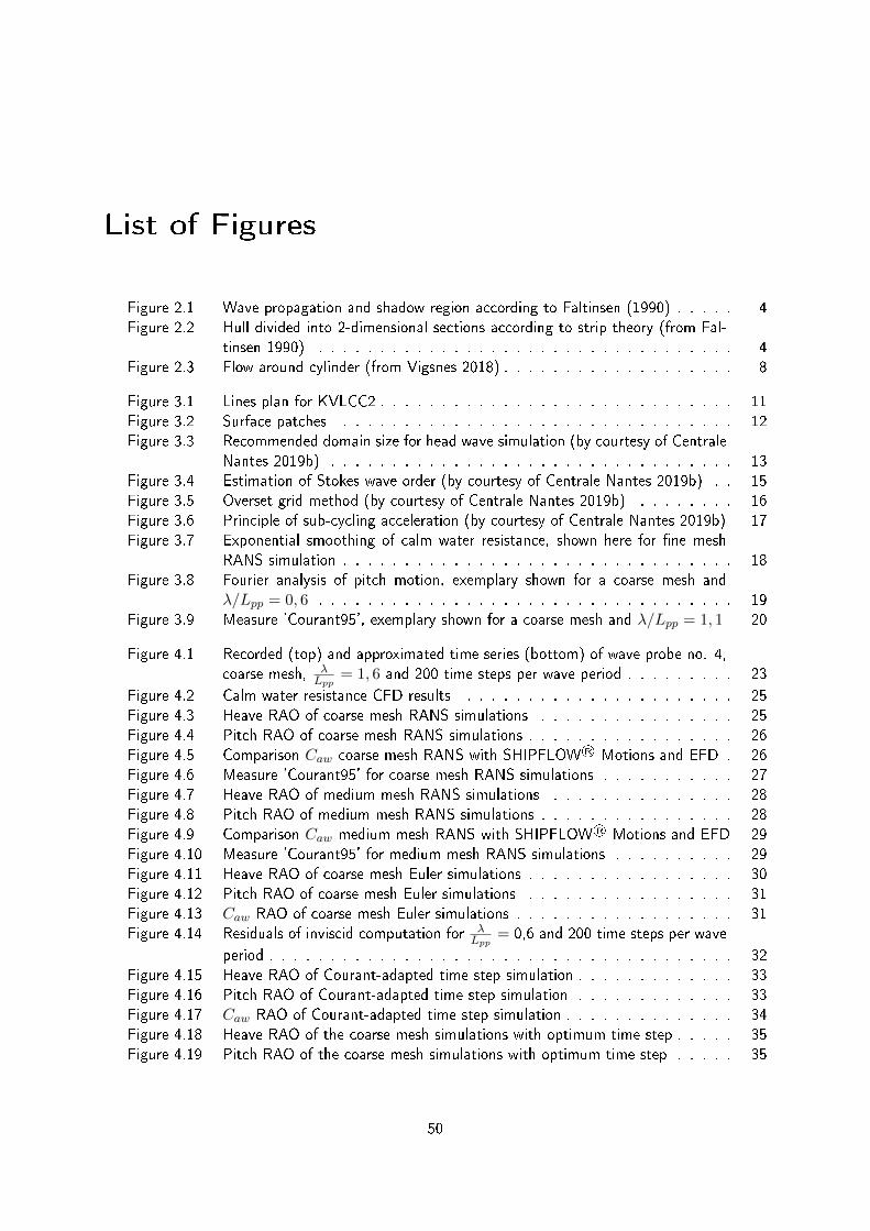
http://www.simman2008.dk/KVLCC/KVLCC2/kvlcc2_geometry.html

http://www.simman2008.dk/KVLCC/KVLCC2/kvlcc2_geometry.html

List of Figures

Figure 2.1 Wave propagation and shadow region according to Faltinsen (1990) . . . . . 4Figure 2.2 Hull divided into 2-dimensional sections according to strip theory (from Fal-

tinsen 1990) . . . . . . . . . . . . . . . . . . . . . . . . . . . . . . . . . . 4Figure 2.3 Flow-around cylinder (from Vigsnes 2018) . . . . . . . . . . . . . . . . . . . 8

Figure 3.1 Lines plan for KVLCC2 . . . . . . . . . . . . . . . . . . . . . . . . . . . . . 11Figure 3.2 Surface patches . . . . . . . . . . . . . . . . . . . . . . . . . . . . . . . . 12Figure 3.3 Recommended domain size for head wave simulation (by courtesy of Centrale

Nantes 2019b) . . . . . . . . . . . . . . . . . . . . . . . . . . . . . . . . . 13Figure 3.4 Estimation of Stokes wave order (by courtesy of Centrale Nantes 2019b) . . 15Figure 3.5 Overset grid method (by courtesy of Centrale Nantes 2019b) . . . . . . . . 16Figure 3.6 Principle of sub-cycling acceleration (by courtesy of Centrale Nantes 2019b) 17Figure 3.7 Exponential smoothing of calm water resistance, shown here for �ne mesh

RANS simulation . . . . . . . . . . . . . . . . . . . . . . . . . . . . . . . . 18Figure 3.8 Fourier analysis of pitch motion, exemplary shown for a coarse mesh and

λ/Lpp = 0, 6 . . . . . . . . . . . . . . . . . . . . . . . . . . . . . . . . . . 19Figure 3.9 Measure 'Courant95', exemplary shown for a coarse mesh and λ/Lpp = 1, 1 20

Figure 4.1 Recorded (top) and approximated time series (bottom) of wave probe no. 4,coarse mesh, λ

Lpp= 1, 6 and 200 time steps per wave period . . . . . . . . . 23

Figure 4.2 Calm water resistance CFD results . . . . . . . . . . . . . . . . . . . . . . 25Figure 4.3 Heave RAO of coarse mesh RANS simulations . . . . . . . . . . . . . . . . 25Figure 4.4 Pitch RAO of coarse mesh RANS simulations . . . . . . . . . . . . . . . . . 26Figure 4.5 Comparison Caw coarse mesh RANS with SHIPFLOW® Motions and EFD . 26Figure 4.6 Measure 'Courant95' for coarse mesh RANS simulations . . . . . . . . . . . 27Figure 4.7 Heave RAO of medium mesh RANS simulations . . . . . . . . . . . . . . . 28Figure 4.8 Pitch RAO of medium mesh RANS simulations . . . . . . . . . . . . . . . . 28Figure 4.9 Comparison Caw medium mesh RANS with SHIPFLOW® Motions and EFD 29Figure 4.10 Measure 'Courant95' for medium mesh RANS simulations . . . . . . . . . . 29Figure 4.11 Heave RAO of coarse mesh Euler simulations . . . . . . . . . . . . . . . . . 30Figure 4.12 Pitch RAO of coarse mesh Euler simulations . . . . . . . . . . . . . . . . . 31Figure 4.13 Caw RAO of coarse mesh Euler simulations . . . . . . . . . . . . . . . . . . 31Figure 4.14 Residuals of inviscid computation for λ

Lpp= 0,6 and 200 time steps per wave

period . . . . . . . . . . . . . . . . . . . . . . . . . . . . . . . . . . . . . . 32Figure 4.15 Heave RAO of Courant-adapted time step simulation . . . . . . . . . . . . . 33Figure 4.16 Pitch RAO of Courant-adapted time step simulation . . . . . . . . . . . . . 33Figure 4.17 Caw RAO of Courant-adapted time step simulation . . . . . . . . . . . . . . 34Figure 4.18 Heave RAO of the coarse mesh simulations with optimum time step . . . . . 35Figure 4.19 Pitch RAO of the coarse mesh simulations with optimum time step . . . . . 35

50

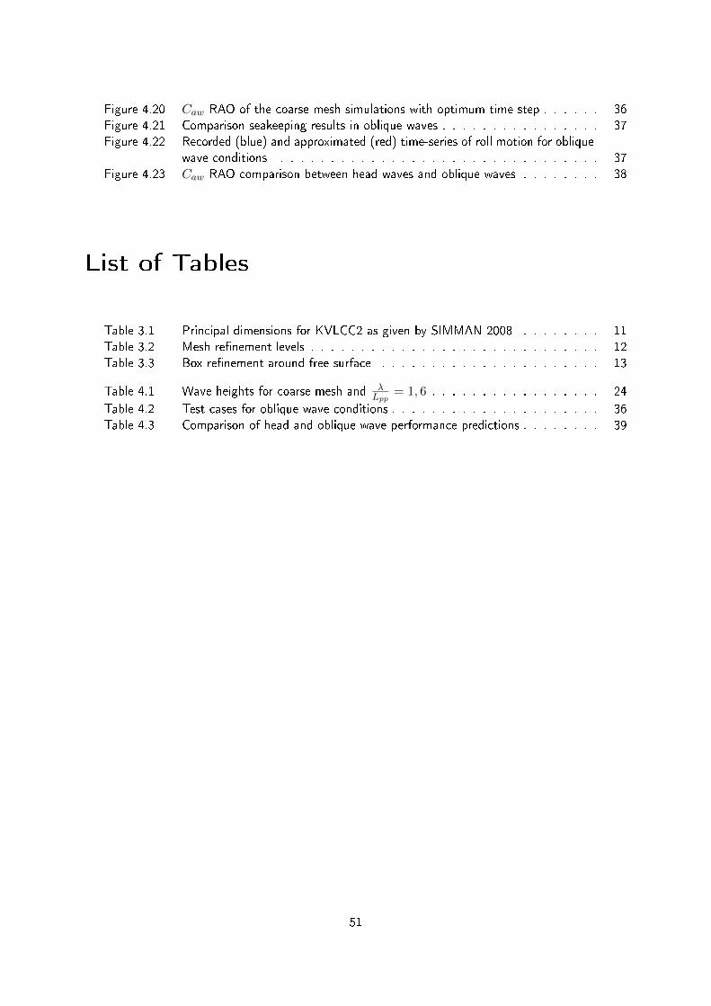
Figure 4.20 Caw RAO of the coarse mesh simulations with optimum time step . . . . . . 36Figure 4.21 Comparison seakeeping results in oblique waves . . . . . . . . . . . . . . . . 37Figure 4.22 Recorded (blue) and approximated (red) time-series of roll motion for oblique

wave conditions . . . . . . . . . . . . . . . . . . . . . . . . . . . . . . . . 37Figure 4.23 Caw RAO comparison between head waves and oblique waves . . . . . . . . 38

List of Tables

Table 3.1 Principal dimensions for KVLCC2 as given by SIMMAN 2008 . . . . . . . . 11Table 3.2 Mesh re�nement levels . . . . . . . . . . . . . . . . . . . . . . . . . . . . . 12Table 3.3 Box re�nement around free surface . . . . . . . . . . . . . . . . . . . . . . 13

Table 4.1 Wave heights for coarse mesh and λLpp

= 1, 6 . . . . . . . . . . . . . . . . . 24

Table 4.2 Test cases for oblique wave conditions . . . . . . . . . . . . . . . . . . . . . 36Table 4.3 Comparison of head and oblique wave performance predictions . . . . . . . . 39

51

Appendix

52

APPENDIX

MATLAB Post-processing script for resistance computations

c l c ;c l e a r a l l ;c l o s e a l l ;

%%MANUALLY − Set inputVes se lSpeed = 1 . 0 4 7 ; %[m/ s ]Smooth i ngFac to rRe s i s t ance = 0 . 9 9 5 ; %[%] How much o f the p r e v i o u s s o l u t i o n s h a l l be keptSmooth ingFac to rP i t ch = 0 . 9 9 5 ; %[%] How much o f the p r e v i o u s s o l u t i o n s h a l l be keptSmooth ingFactorHeave = 0 . 9 9 5 ; %[%] How much o f the p r e v i o u s s o l u t i o n s h h a l l be keptReverseApproach = 1 ; %0 i f s t a r t smooth ing from t=0; 1 i f s t a r t smooth ing

from t=endAvgF r a c t i o nRe s i s t a n c e = 0 . 3 ; %[%] P ropo r t i o n o f the r e co r d ed r e s i s t a n c e data tha t

s h a l l be ave ragedAvgF ra c t i onP i t ch = 0 . 3 ; %[%] P ropo r t i o n o f the r e co r d ed p i t c h data tha t s h a l l

be ave ragedAvgFract ionHeave = 0 . 3 ; %[%] P ropo r t i o n o f the r e co r d ed heave data tha t s h a l l

be ave ragedf i l e n ame = ' computed_data . dat ' ;

%%AUTOMATIC − Post−proces s ing data%Import f i l ecomputeddata = i m p o r t f i l e ( f i l e n ame ) ;%Conver t P i t ch i n t o degcomputeddata . Ry1Vesse l = rad2deg ( computeddata . Ry1Vesse l ) ;

%Find f i r s t t ime s t ep wi th f u l l speedi n d e xFu l l S p e e d = 1 ;wh i l e computeddata . VxVesse l ( i n d e xFu l l S p e e d ) < Ves s e lSpeed

i n d e xFu l l S p e e d = i nd e xFu l l S p e ed + 1 ;end

i f ReverseApproach == 0%Copy t ime s e r i e s b e f o r e f u l l speed i s r eachedf o r i =1:( i ndexFu l l Spe ed −1)

computeddata . SmoothedRes i s tance ( i ) = computeddata . FxVe s s e l ( i ) ;computeddata . SmoothedPitch ( i ) = computeddata . Ry1Vesse l ( i ) ;computeddata . SmoothedHeave ( i ) = computeddata . Tz0Vesse l ( i ) ;

end

%Smooth data a f t e r f u l l speed i s r eachedf o r j=i nd e xFu l l S p e ed : l e n g t h ( computeddata .T)

computeddata . SmoothedRes i s tance ( j ) = computeddata . SmoothedRes i s tance ( j −1)*Smooth i ngFac to rRe s i s t ance + computeddata . FxVe s s e l ( j )*(1−Smooth i ngFac to rRe s i s t ance ) ;

computeddata . SmoothedPitch ( j ) = computeddata . SmoothedPitch ( j −1)*Smooth ingFac to rP i t ch + computeddata . Ry1Vesse l ( j )*(1−Smooth ingFac to rP i t ch ) ;

computeddata . SmoothedHeave ( j ) = computeddata . SmoothedHeave ( j −1)*Smooth ingFactorHeave + computeddata . Tz0Vesse l ( j )*(1−Smooth ingFactorHeave ) ;

end

e l s e i f ReverseApproach == 1%Copy t ime s e r i e s b e f o r e f u l l speed i s r eachedn=l e ng t h ( computeddata .T) ;computeddata . SmoothedRes i s tance = computeddata . FxVe s s e l ;computeddata . SmoothedPitch = computeddata . Ry1Vesse l ;computeddata . SmoothedHeave = computeddata . Tz0Vesse l ;%Smooth data a f t e r f u l l speed i s r eachedf o r j =2:(n−1)

computeddata . SmoothedRes i s tance (n−j ) = computeddata . SmoothedRes i s tance (n−j +1)*Smooth i ngFac to rRe s i s t ance + computeddata . FxVe s s e l ( n−j )*(1−Smooth i ngFac to rRe s i s t ance ) ;

computeddata . SmoothedPitch (n−j ) = computeddata . SmoothedPitch (n−j +1)*Smooth ingFac to rP i t ch + computeddata . Ry1Vesse l ( n−j )*(1−Smooth ingFac to rP i t ch ) ;

computeddata . SmoothedHeave (n−j ) = computeddata . SmoothedHeave (n−j +1)*Smooth ingFactorHeave + computeddata . Tz0Vesse l ( n−j )*(1−Smooth ingFactorHeave ) ;

a

APPENDIX

endend

% Average smoothed q u a n t i t i e sAvgRe s i s t a n c eS t a r t I n d e x = round ( l e n g t h ( computeddata .T)*(1−AvgF r a c t i o nRe s i s t a n c e ) ) ;AvgP i t chS t a r t I nd e x = round ( l e n g t h ( computeddata .T)*(1−AvgF ra c t i onP i t ch ) ) ;AvgHeaveSta r t Index = round ( l e n g t h ( computeddata .T)*(1−AvgFract ionHeave ) ) ;

AvgRes i s t ance = mean ( computeddata . SmoothedRes i s tance ( AvgRe s i s t a n c eS t a r t I n d e x : end ) ) ;AvgPitch = mean ( computeddata . SmoothedPitch ( AvgP i t c hS t a r t I nd e x : end ) ) ;AvgHeave = mean ( computeddata . SmoothedHeave ( AvgHeaveSta r t Index : end ) ) ;

%% Plot func t i on sf i g u r e ( 'Name ' , ' Re s i s t a n c e ' )p l o t ( computeddata .T, computeddata . FxVe s s e l )ho ld onp l o t ( computeddata .T, computeddata . SmoothedRes i s tance )l i n e ( [ computeddata .T( AvgRe s i s t a n c eS t a r t I n d e x ) computeddata .T( end ) ] , [ AvgRes i s t ance

AvgRes i s t ance ] , ' Co lo r ' , ' b l a ck ' , 'DisplayName ' , ' Average R e s i s t a n c e ' ) ;x l a b e l ( ' t ime [ s ] ' ) ;y l a b e l ( ' Re s i s t a n c e [N] ' ) ;l e g end ( 'Computed Re s i s t a n c e ' , ' Smoothed Re s i s t a n c e ' , ' Average R e s i s t a n c e ' )

f i g u r e ( 'Name ' , ' P i t ch ' )p l o t ( computeddata .T, computeddata . Ry1Vesse l )ho ld onp l o t ( computeddata .T, computeddata . SmoothedPitch )l i n e ( [ computeddata .T( AvgP i t c hS t a r t I nd e x ) computeddata .T( end ) ] , [ AvgPitch AvgPitch ] , ' Co lo r

' , ' b l a ck ' , 'DisplayName ' , ' Average P i t ch ' ) ;x l a b e l ( ' t ime [ s ] ' ) ;y l a b e l ( ' P i t ch ang l e [ ° ] ' ) ;l e g end ( 'Computed P i t ch ' , ' Smoothed P i t ch ' , ' Average P i t ch ' )

f i g u r e ( 'Name ' , 'Heave ' )p l o t ( computeddata .T, computeddata . Tz0Vesse l )ho ld onp l o t ( computeddata .T, computeddata . SmoothedHeave )l i n e ( [ computeddata .T( AvgHeaveSta r t Index ) computeddata .T( end ) ] , [ AvgHeave AvgHeave ] , ' Co lo r

' , ' b l a ck ' , 'DisplayName ' , ' Average Heave ' ) ;x l a b e l ( ' t ime [ s ] ' ) ;y l a b e l ( 'Heave [m] ' ) ;l e g end ( 'Computed Heave ' , ' Smoothed Heave ' , ' Average Heave ' )

f i g u r e ( 'Name ' , ' Courant number ' )p l o t ( computeddata .T, computeddata . Courant )ho ld onx l a b e l ( ' t ime [ s ] ' ) ;y l a b e l ( ' Courant number ' ) ;l e g end ( 'Computed t ime s e r i e s ' )

%% Pr int r e s u l td i s p ( s t r c a t ( ' Average R e s i s t a n c e [N] ove r the l a s t ' , { ' ' } , num2str ( AvgF r a c t i o nRe s i s t a n c e

*100) , '%: ' ) )d i s p ( AvgRes i s t ance )d i s p ( s t r c a t ( ' Average P i t ch ang l e [ ° ] o ve r the l a s t ' , { ' ' } , num2str ( AvgF ra c t i onP i t ch *100)

, '%: ' ) )d i s p ( AvgPitch )d i s p ( s t r c a t ( ' Average Heave [m] ove r the l a s t ' , { ' ' } , num2str ( AvgFract ionHeave *100) , '%: '

) )d i s p ( AvgHeave )

b

APPENDIX

MATLAB Post-processing script for seakeeping simulations


%%MANUALLY − Set inputWavePeriod = 1 . 9716 ; %[ s ]Ve s s e lSpeed = 1 . 0 4 7 ; %[m/ s ]WaveAngle = 20 ; %[ deg ] 0=head wavesWavesToRecord = 10 ; %Number o f encounte r ed waves to a n a l y s ef i l e n ame = ' computed_data . dat ' ;UseCourant = 1 ; %For i n v i s c i d computat ions s e t to 0F r e eRo l l = 1 ; %s e t 1 i f f r e e to r o l lFreeYaw = 0 ; %s e t 1 i f f r e e to yaw

%%AUTOMATIC − Post−proces s ing data%Import f i l ecomputeddata = i m p o r t f i l e ( f i l e n ame ) ;%Conver t P i tch , R o l l and Yaw i n t o degcomputeddata . Ry1Vesse l = rad2deg ( computeddata . Ry1Vesse l ) ;i f FreeYaw==1

computeddata . Rz0Ves se l = rad2deg ( computeddata . Rz0Ves se l ) ;endi f F r e eRo l l==1

computeddata . Rx2Vesse l = rad2deg ( computeddata . Rx2Vesse l ) ;end

%Conver t Fx and Fy i n t o Cardan−r o t a t e d c o o r d i n a t e si f WaveAngle ~=0

FxO r i g i n a l = computeddata . FxVe s s e l ;F yO r i g i n a l = computeddata . FyVe s s e l ;computeddata . FxVe s s e l = FxO r i g i n a l * cosd (WaveAngle ) − FyO r i g i n a l * s i n d (WaveAngle ) ;computeddata . FyVe s s e l = FyO r i g i n a l * cosd (WaveAngle ) + FxO r i g i n a l * s i n d (WaveAngle ) ;

end

f e = 1/WavePeriod + ( Ves s e lSpeed * cosd (WaveAngle ) ) /(9 .81/2/ p i *WavePeriod ^2) ; %[ Hz ]Te = 1/ f e ; %[ s ]

% p l o t i n pu t datap l o t ( computeddata .T, computeddata . FxVe s s e l )t i t l e ( 'Time−h i s t o r y ' ) ;x l a b e l ( ' t ime [ s ] ' ) ;y l a b e l ( 'Fx ' ) ;

% cut data , s e t t ime i n [ s ]setCutTime = computeddata .T( end )−Te*WavesToRecord ;CutTimeIndex = f i n d ( computeddata .T>setCutTime , 1 ) ;CutData = computeddata ( CutTimeIndex : end , : ) ;CutData .T = CutData .T−CutData .T(1 ) ;computeddata .T = computeddata .T−computeddata .T( CutTimeIndex ) ;

% Fou r i e r t r a n s f o rma t i o n%Re s i s t a n c ef o u r i e r F u n c t i o nR e s i s t a n c e = f i t ( CutData .T, CutData . FxVesse l , ' f o u r i e r 8 ' ) ;c o e f f i c i e n t s R e s i s t a n c e = c o e f f v a l u e s ( f o u r i e r F u n c t i o nR e s i s t a n c e ) ;%Ex t r a c t c o r r e c t f r e qu en c yomegaRes i s tance = c o e f f i c i e n t s R e s i s t a n c e ( end ) ;counte rOmegaRes i s tance = 1 ;wh i l e ( ( omegaRes i s tance * counte rOmegaRes i s tance ) <0.95*(2* p i * f e ) )

counte rOmegaRes i s tance = counte rOmegaRes i s tance + 1 ;endd i s p ( ' Encounter f r e qu en c y f o r r e s i s t a n c e [ rad / s ] : ' )d i s p (2* p i * f e )d i s p ( 'CHECK: F o u r i e r f r e qu en c y f o r r e s i s t a n c e [ rad / s ] : ' )d i s p ( omegaRes i s tance * counte rOmegaRes i s tance )

c

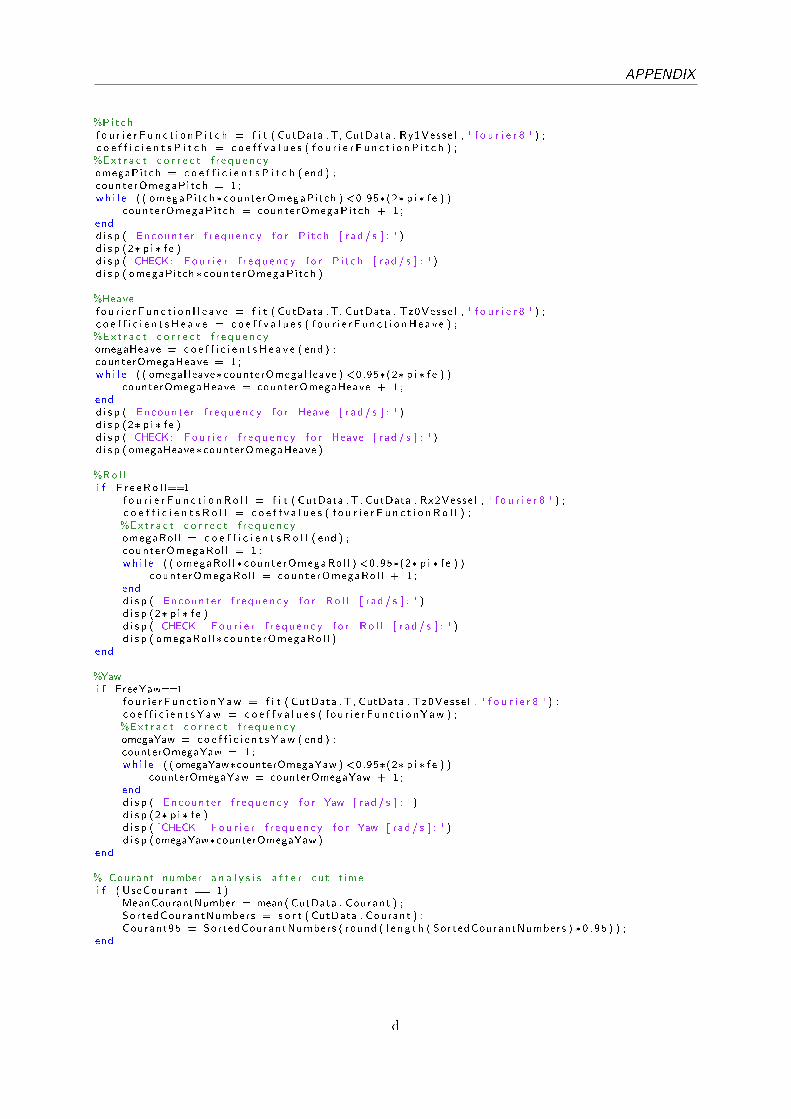
APPENDIX

%Pi t chf o u r i e r F u n c t i o nP i t c h = f i t ( CutData .T, CutData . Ry1Vesse l , ' f o u r i e r 8 ' ) ;c o e f f i c i e n t s P i t c h = c o e f f v a l u e s ( f o u r i e r F u n c t i o nP i t c h ) ;%Ex t r a c t c o r r e c t f r e qu en c yomegaPitch = c o e f f i c i e n t s P i t c h ( end ) ;counterOmegaPitch = 1 ;wh i l e ( ( omegaPitch* counterOmegaPitch ) <0.95*(2* p i * f e ) )

counterOmegaPitch = counterOmegaPitch + 1 ;endd i s p ( ' Encounter f r e qu en c y f o r P i t ch [ rad / s ] : ' )d i s p (2* p i * f e )d i s p ( 'CHECK: F o u r i e r f r e qu en c y f o r P i t ch [ rad / s ] : ' )d i s p ( omegaPitch* counterOmegaPitch )

%Heavef o u r i e r F un c t i o nHea v e = f i t ( CutData .T, CutData . Tz0Vesse l , ' f o u r i e r 8 ' ) ;c o e f f i c i e n t s H e a v e = c o e f f v a l u e s ( f o u r i e r F un c t i o nHea v e ) ;%Ex t r a c t c o r r e c t f r e qu en c yomegaHeave = c o e f f i c i e n t s H e a v e ( end ) ;counterOmegaHeave = 1 ;wh i l e ( ( omegaHeave* counterOmegaHeave ) <0.95*(2* p i * f e ) )

counterOmegaHeave = counterOmegaHeave + 1 ;endd i s p ( ' Encounter f r e qu en c y f o r Heave [ rad / s ] : ' )d i s p (2* p i * f e )d i s p ( 'CHECK: F o u r i e r f r e qu en c y f o r Heave [ rad / s ] : ' )d i s p ( omegaHeave* counterOmegaHeave )

%Ro l li f F r e eRo l l==1

f o u r i e r F u n c t i o n R o l l = f i t ( CutData .T, CutData . Rx2Vesse l , ' f o u r i e r 8 ' ) ;c o e f f i c i e n t s R o l l = c o e f f v a l u e s ( f o u r i e r F u n c t i o n R o l l ) ;%Ex t r a c t c o r r e c t f r e qu en c yomegaRol l = c o e f f i c i e n t s R o l l ( end ) ;counterOmegaRol l = 1 ;wh i l e ( ( omegaRol l * counterOmegaRol l ) <0.95*(2* p i * f e ) )

counterOmegaRol l = counterOmegaRol l + 1 ;endd i s p ( ' Encounter f r e qu en c y f o r R o l l [ rad / s ] : ' )d i s p (2* p i * f e )d i s p ( 'CHECK: F o u r i e r f r e qu en c y f o r R o l l [ rad / s ] : ' )d i s p ( omegaRol l * counterOmegaRol l )

end

%Yawi f FreeYaw==1

fou r i e rFunc t i onYaw = f i t ( CutData .T, CutData . Tz0Vesse l , ' f o u r i e r 8 ' ) ;c o e f f i c i e n t s Y aw = c o e f f v a l u e s ( f ou r i e rFunc t i onYaw ) ;%Ex t r a c t c o r r e c t f r e qu en c yomegaYaw = co e f f i c i e n t s Y aw ( end ) ;counterOmegaYaw = 1 ;wh i l e ( ( omegaYaw*counterOmegaYaw ) <0.95*(2* p i * f e ) )

counterOmegaYaw = counterOmegaYaw + 1 ;endd i s p ( ' Encounter f r e qu en c y f o r Yaw [ rad / s ] : ' )d i s p (2* p i * f e )d i s p ( 'CHECK: F o u r i e r f r e qu en c y f o r Yaw [ rad / s ] : ' )d i s p (omegaYaw*counterOmegaYaw )

end

% Courant number a n a l y s i s a f t e r cut t imei f ( UseCourant == 1)

MeanCourantNumber = mean ( CutData . Courant ) ;SortedCourantNumbers = s o r t ( CutData . Courant ) ;Courant95 = SortedCourantNumbers ( round ( l e n g t h ( SortedCourantNumbers ) *0 .95 ) ) ;

end

d

APPENDIX

%% Plot func t i on sf i g u r e ( 'Name ' , ' Re s i s t a n c e ' )p l o t ( computeddata .T, computeddata . FxVe s s e l )ho ld onp l o t ( f o u r i e r F u n c t i o nR e s i s t a n c e )l i n e ( [ 0 0 ] , ge t ( gca , ' y l im ' ) , ' Co lo r ' , ' b l a ck ' , 'DisplayName ' , ' cut t ime ' ) ;x l a b e l ( ' t ime [ s ] ' ) ;y l a b e l ( ' Re s i s t a n c e [N] ' ) ;l e g end ( 'Computed t ime s e r i e s ' , ' Fou r i e r f u n c t i o n ' , ' cut t ime ' )

i f WaveAngle~=0f i g u r e ( 'Name ' , 'Fy ' )p l o t ( computeddata .T, computeddata . FyVe s s e l )ho ld onx l a b e l ( ' t ime [ s ] ' ) ;y l a b e l ( 'Fy [N] ' ) ;l e g end ( 'Computed t ime s e r i e s ' )

end

f i g u r e ( 'Name ' , ' P i t ch ' )p l o t ( computeddata .T, computeddata . Ry1Vesse l )ho ld onp l o t ( f o u r i e r F u n c t i o nP i t c h )l i n e ( [ 0 0 ] , ge t ( gca , ' y l im ' ) , ' Co lo r ' , ' b l a ck ' , 'DisplayName ' , ' cut t ime ' ) ;x l a b e l ( ' t ime [ s ] ' ) ;y l a b e l ( ' P i t ch ang l e [ ° ] ' ) ;l e g end ( 'Computed t ime s e r i e s ' , ' Fou r i e r f u n c t i o n ' , ' cut t ime ' )

f i g u r e ( 'Name ' , 'Heave ' )p l o t ( computeddata .T, computeddata . Tz0Vesse l )ho ld onp l o t ( f o u r i e r F un c t i o nHea v e )l i n e ( [ 0 0 ] , ge t ( gca , ' y l im ' ) , ' Co lo r ' , ' b l a ck ' , 'DisplayName ' , ' cut t ime ' ) ;x l a b e l ( ' t ime [ s ] ' ) ;y l a b e l ( 'Heave [m] ' ) ;l e g end ( 'Computed t ime s e r i e s ' , ' Fou r i e r f u n c t i o n ' , ' cut t ime ' )

i f F r e eRo l l==1f i g u r e ( 'Name ' , ' Ro l l ' )p l o t ( computeddata .T, computeddata . Rx2Vesse l )ho ld onp l o t ( f o u r i e r F u n c t i o n R o l l )l i n e ( [ 0 0 ] , ge t ( gca , ' y l im ' ) , ' Co lo r ' , ' b l a ck ' , 'DisplayName ' , ' cut t ime ' ) ;x l a b e l ( ' t ime [ s ] ' ) ;y l a b e l ( ' Ro l l ang l e [ ° ] ' ) ;l e g end ( 'Computed t ime s e r i e s ' , ' Fou r i e r f u n c t i o n ' , ' cut t ime ' )

end

i f FreeYaw==1f i g u r e ( 'Name ' , 'Yaw ' )p l o t ( computeddata .T, computeddata . Rz0Ves se l )ho ld onp l o t ( f ou r i e rFunc t i onYaw )l i n e ( [ 0 0 ] , ge t ( gca , ' y l im ' ) , ' Co lo r ' , ' b l a ck ' , 'DisplayName ' , ' cut t ime ' ) ;x l a b e l ( ' t ime [ s ] ' ) ;y l a b e l ( 'Yaw ang l e [ ° ] ' ) ;l e g end ( 'Computed t ime s e r i e s ' , ' Fou r i e r f u n c t i o n ' , ' cut t ime ' )

end

i f ( UseCourant == 1)f i g u r e ( 'Name ' , ' Courant number ' )p l o t ( computeddata .T, computeddata . Courant )ho ld onl i n e ( ge t ( gca , ' x l im ' ) , [ Courant95 Courant95 ] , ' Co lo r ' , ' r ed ' , 'DisplayName ' , ' cut t ime ' ) ;l i n e ( [ 0 0 ] , ge t ( gca , ' y l im ' ) , ' Co lo r ' , ' b l a ck ' , 'DisplayName ' , ' cut t ime ' ) ;x l a b e l ( ' t ime [ s ] ' ) ;y l a b e l ( ' Courant number ' ) ;

e

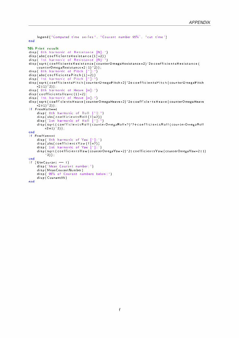
APPENDIX

l e g end ( 'Computed t ime s e r i e s ' , ' Courant number 95% ' , ' cut t ime ' )end

%% Pr int r e s u l td i s p ( ' 0 th harmonic o f R e s i s t a n c e [N ] : ' )d i s p ( abs ( c o e f f i c i e n t s R e s i s t a n c e (1 ) *2) )d i s p ( ' 1 s t harmonic o f R e s i s t a n c e [N ] : ' )d i s p ( s q r t ( c o e f f i c i e n t s R e s i s t a n c e ( counte rOmegaRes i s tance *2)^2+c o e f f i c i e n t s R e s i s t a n c e (

counte rOmegaRes i s tance *2+1)^2) ) ;d i s p ( ' 0 th harmonic o f P i t ch [ ° ] : ' )d i s p ( abs ( c o e f f i c i e n t s P i t c h (1 ) *2) )d i s p ( ' 1 s t harmonic o f P i t ch [ ° ] : ' )d i s p ( s q r t ( c o e f f i c i e n t s P i t c h ( counterOmegaPitch *2)^2+ c o e f f i c i e n t s P i t c h ( counterOmegaPitch

*2+1)^2) ) ;d i s p ( ' 0 th harmonic o f Heave [m] : ' )d i s p ( c o e f f i c i e n t s H e a v e (1 ) *2) ;d i s p ( ' 1 s t harmonic o f Heave [m] : ' )d i s p ( s q r t ( c o e f f i c i e n t s H e a v e ( counterOmegaHeave *2)^2+c o e f f i c i e n t s H e a v e ( counterOmegaHeave

*2+1)^2) ) ;i f F r e eRo l l==1

d i s p ( ' 0 th harmonic o f R o l l [ ° ] : ' )d i s p ( abs ( c o e f f i c i e n t s R o l l ( 1 ) *2) )d i s p ( ' 1 s t harmonic o f R o l l [ ° ] : ' )d i s p ( s q r t ( c o e f f i c i e n t s R o l l ( counterOmegaRol l *2)^2+ c o e f f i c i e n t s R o l l ( counterOmegaRol l

*2+1)^2) ) ;endi f FreeYaw==1

d i s p ( ' 0 th harmonic o f Yaw [ ° ] : ' )d i s p ( abs ( c o e f f i c i e n t s Y aw (1) *2) )d i s p ( ' 1 s t harmonic o f Yaw [ ° ] : ' )d i s p ( s q r t ( c o e f f i c i e n t s Y aw ( counterOmegaYaw *2)^2+c o e f f i c i e n t s Y aw ( counterOmegaYaw*2+1)

^2) ) ;endi f ( UseCourant == 1)

d i s p ( 'Mean Courant number : ' )d i s p (MeanCourantNumber )d i s p ( '95% of Courant numbers below : ' )d i s p ( Courant95 )

end

f

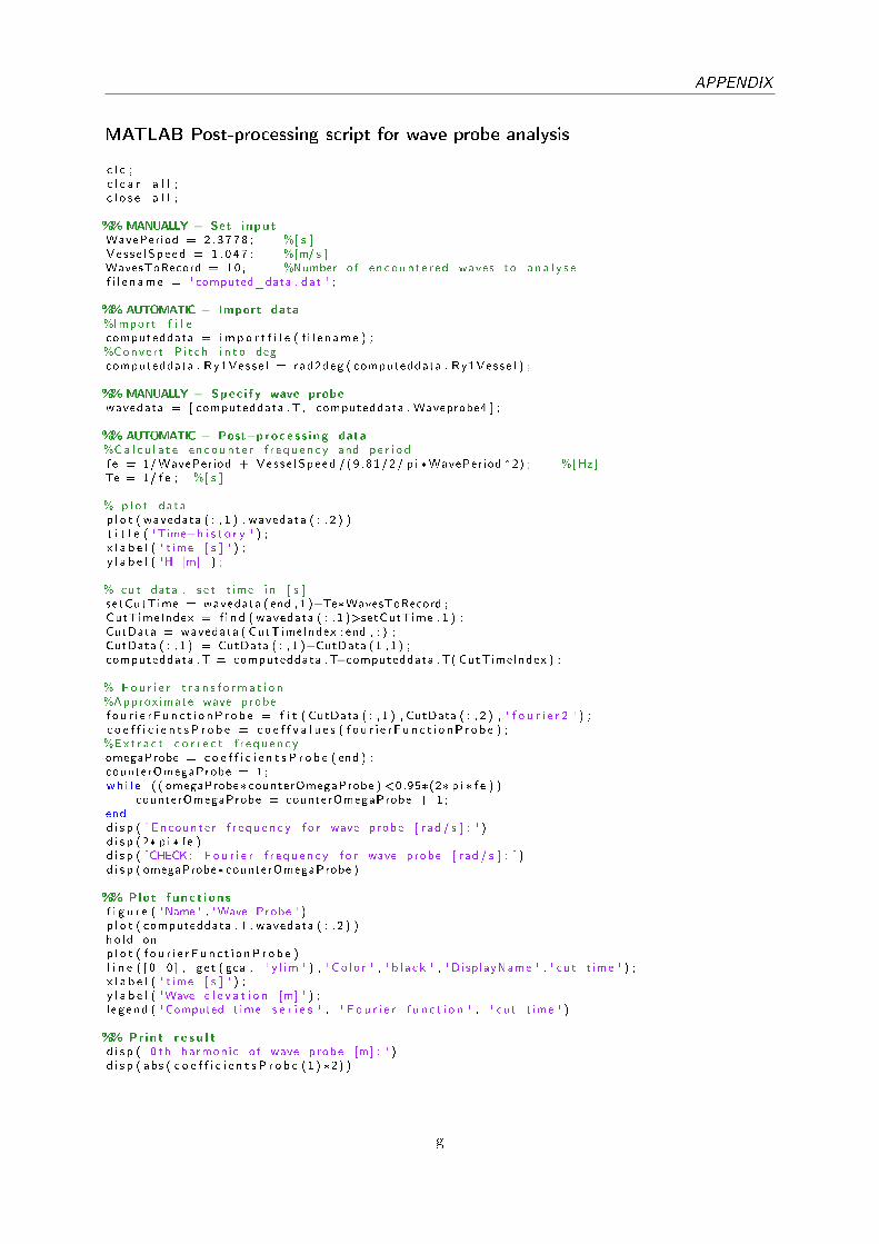
APPENDIX

MATLAB Post-processing script for wave probe analysis


%%MANUALLY − Set inputWavePeriod = 2 . 3778 ; %[ s ]Ve s s e lSpeed = 1 . 0 4 7 ; %[m/ s ]WavesToRecord = 10 ; %Number o f encounte r ed waves to a n a l y s ef i l e n ame = ' computed_data . dat ' ;

%%AUTOMATIC − Import data%Import f i l ecomputeddata = i m p o r t f i l e ( f i l e n ame ) ;%Conver t P i t ch i n t o degcomputeddata . Ry1Vesse l = rad2deg ( computeddata . Ry1Vesse l ) ;

%%MANUALLY − Spec i f y wave probewavedata = [ computeddata .T, computeddata . Waveprobe4 ] ;

%%AUTOMATIC − Post−proces s ing data%Ca l c u l a t e encoun t e r f r e qu enc y and p e r i o df e = 1/WavePeriod + Ves se lSpeed /(9 .81/2/ p i *WavePeriod ^2) ; %[ Hz ]Te = 1/ f e ; %[ s ]

% p l o t datap l o t ( wavedata ( : , 1 ) , wavedata ( : , 2 ) )t i t l e ( 'Time−h i s t o r y ' ) ;x l a b e l ( ' t ime [ s ] ' ) ;y l a b e l ( 'H [m] ' ) ;

% cut data , s e t t ime i n [ s ]setCutTime = wavedata ( end , 1 )−Te*WavesToRecord ;CutTimeIndex = f i n d ( wavedata ( : , 1 )>setCutTime , 1 ) ;CutData = wavedata ( CutTimeIndex : end , : ) ;CutData ( : , 1 ) = CutData ( : , 1 )−CutData (1 , 1 ) ;computeddata .T = computeddata .T−computeddata .T( CutTimeIndex ) ;

% Fou r i e r t r a n s f o rma t i o n%Approx imate wave probef o u r i e r F u n c t i o nP r o b e = f i t ( CutData ( : , 1 ) , CutData ( : , 2 ) , ' f o u r i e r 2 ' ) ;c o e f f i c i e n t s P r o b e = c o e f f v a l u e s ( f o u r i e r F u n c t i o nP r o b e ) ;%Ex t r a c t c o r r e c t f r e qu en c yomegaProbe = c o e f f i c i e n t s P r o b e ( end ) ;counterOmegaProbe = 1 ;wh i l e ( ( omegaProbe* counterOmegaProbe ) <0.95*(2* p i * f e ) )

counterOmegaProbe = counterOmegaProbe + 1 ;endd i s p ( ' Encounter f r e qu en c y f o r wave probe [ rad / s ] : ' )d i s p (2* p i * f e )d i s p ( 'CHECK: F o u r i e r f r e qu en c y f o r wave probe [ rad / s ] : ' )d i s p ( omegaProbe* counterOmegaProbe )

%% Plot func t i on sf i g u r e ( 'Name ' , 'Wave Probe ' )p l o t ( computeddata .T, wavedata ( : , 2 ) )ho ld onp l o t ( f o u r i e r F u n c t i o nP r o b e )l i n e ( [ 0 0 ] , ge t ( gca , ' y l im ' ) , ' Co lo r ' , ' b l a ck ' , 'DisplayName ' , ' cut t ime ' ) ;x l a b e l ( ' t ime [ s ] ' ) ;y l a b e l ( 'Wave e l e v a t i o n [m] ' ) ;l e g end ( 'Computed t ime s e r i e s ' , ' Fou r i e r f u n c t i o n ' , ' cut t ime ' )

%% Pr int r e s u l td i s p ( ' 0 th harmonic o f wave probe [m] : ' )d i s p ( abs ( c o e f f i c i e n t s P r o b e (1 ) *2) )

g

APPENDIX

d i s p ( ' 1 s t harmonic o f wave probe [m] : ' )d i s p ( s q r t ( c o e f f i c i e n t s P r o b e ( counterOmegaProbe *2)^2+c o e f f i c i e n t s P r o b e ( counterOmegaProbe

*2+1)^2) ) ;d i s p ( 'Measured wave h e i g h t [m] : ' )d i s p ( s q r t ( c o e f f i c i e n t s P r o b e ( counterOmegaProbe *2)^2+c o e f f i c i e n t s P r o b e ( counterOmegaProbe

*2+1)^2) *2) ;

h

APPENDIX

Computers used for computations

Computer name Description CPUs Cores Tot cores GB RAM

Lin05 Dell R710,X5690, 3.3 Ghz 2 6 24 148

Lin11 Dell R820, E54627V2, 3.3 Ghz 4 8 32 256

Lin14 Dell R640, Intel Xeon Gold 6142 2.6 Ghz 2 16 32 192

XPS-12 Dell XPS-12, Intel Core i7-4500U, 1.8 Ghz 1 4 4 8

Workstation Intel Core i7-2600, 3.4 Ghz 1 8 8 12

Chalmers exact con�guration unknown, faster than Lin14 32

i

APPENDIX

Compilation of results

Calm-water simulations

Simulation No. 1 2 3 4 5 6

Set-up

Folder name KVLCC2_Res

_RANS_coarse

_v2

KVLCC2_Res

_RANS_medium

_v1

KVLCC2_Res

_RANS_�ne

_v1

KVLCC2_Re

s_Euler_coarse

_v2

KVLCC2_Res

_Euler_medium

_v1

KVLCC2_Res

_Euler_�ne

_v1

Computer XPS-12 XPS-12 XPS-12 XPS-12 XPS-12 XPS-12

Cores 4 4 4 4 4 4

Flow/turbulence model SST-Menter SST-Menter SST-Menter Euler Euler Euler

Mesh re�nement coarse medium �ne coarse medium �ne

Number of cells 378.144 839.388 1.103.657 215.466 571.823 770.206

Motions free to heave

and pitch

free to heave

and pitch

free to heave

and pitch

free to heave

and pitch

free to heave

and pitch

free to heave

and pitch

Time-step [s] 0,0275 0,0275 0,0275 0,0275 0,0275 0,0275

Number of non-linear

iterations

5 5 5 5 5 5

Result

Computational time [h] 6,4 16,0 19,4 4,0 10,7 11,6

Total core-h 25,6 64,0 77,6 16,0 42,8 46,4

RT for full body [N] 18,262 17,995 17,916 3,140 2,286 2,035

Dynamic wetted

surface [m2]

8,0838 8,0838 8,0838 8,0838 8,0838 8,0838

Trim angle [°] 0,13 0,13 0,13 0,13 0,13 0,13

speed [m/s] 1,047 1,047 1,047 1,047 1,047 1,047

kin. Viscosity [m2/s] 1,1386E-06 1,1386E-06 1,1386E-06 1,1386E-06 1,1386E-06 1,1386E-06

Re 5.073.381 5.073.381 5.073.381 5.073.381 5.073.381 5.073.381

cF0 3,388E-03 3,388E-03 3,388E-03 3,388E-03 3,388E-03 3,388E-03

cF 3,963E-03 3,963E-03 3,963E-03 3,963E-03 3,963E-03 3,963E-03

water density [kg/m3] 999,1026 999,1026 999,1026 999,1026 999,1026 999,1026

RF0[N] 14,996 14,996 14,996 14,996 14,996 14,996

RF [N] 17,545 17,545 17,545 17,545 17,545 17,545

RR [N] 0,716 0,449 0,371 3,140 2,286 2,035

cR 1,618E-04 1,015E-04 8,372E-05 7,093E-04 5,165E-04 4,597E-04

cT 4,125E-03 4,065E-03 4,047E-03 7,093E-04 5,165E-04 4,597E-04

Di�erence to

respective �ne mesh

[%]

1,93% 0,44% 0,00% 54,31% 12,36% 0,00%

j

APPENDIX

Seakeeping simulations

Simulation No. 7 8 9 10 11 12 13

Set-up

Folder name KVLCC2_Sea_RANS_coarse_v4

Computation dT100 dT50 dT50Courant15 dT150 dT200 dT400 dT25

Computer Workstation Lin14 Lin11 Lin11 Lin14 Lin14 Lin05

Cores 8 32 32 32 32 32 12

Flow/turbulence model SST-Menter SST-Menter SST-Menter SST-Menter SST-Menter SST-Menter SST-Menter

Wave period [s] 1,9716 1,9716 1,9716 1,9716 1,9716 1,9716 1,9716

Wave length [m] 6,069 6,069 6,069 6,069 6,069 6,069 6,069

Wave height (H=2A) [m] 0,0607 0,0607 0,0607 0,0607 0,0607 0,0607 0,0607

Encounter period [s] 1,4712 1,4712 1,4712 1,4712 1,4712 1,4712 1,4712

Mesh re�nement coarse coarse coarse coarse coarse coarse coarse

Number of cells 677.976 677.976 677.976 677.976 677.976 677.976 677.976

Motions free to

heave and

pitch

free to

heave and

pitch

free to

heave and

pitch

free to

heave and

pitch

free to

heave and

pitch

free to

heave and

pitch

free to

heave and

pitch

Time-step [s] 0,019726 0,039432 0,039432 0,013144 0,009858 0,004929 0,07886

Max # of sub-cycles 1 1 1 1 1 1 8

Time steps per wave period 100 50 50 150 200 400 25

Time steps per encounter

period

75 37 37 112 149 298 19

Encountering angle [°] 180 180 180 180 180 180 180

speed [m/s] 1,047 1,047 1,047 1,047 1,047 1,047 1,047

kin. Viscosity [m2/s] 1,1386E-06 1,1386E-06 1,1386E-06 1,1386E-06 1,1386E-06 1,1386E-06 1,1386E-06

water density [kg/m3] 999,1026 999,1026 999,1026 999,1026 999,1026 999,1026 999,1026

Results

Computational time [h] 43,2 1,5 7,2 18,65 4,5 12,1 stopped

Core-h 345,6 48 230,4 596,8 144 387,2

corresponding cT,cw 4,125E-03 4,125E-03 4,125E-03 4,125E-03 4,125E-03 4,125E-03 4,125E-03

corresponding RT,cw 18,262 18,262 18,262 18,262 18,262 18,262 18,262

encountered waves to be

analyzed

10 10 10 10 10 10

0th harmonic of RT [N] 59,3993 61,1126 61,1797 60,8592 61,2677 61,6932

Raw [N] 11,438 12,295 12,328 12,168 12,372 12,585

1st harmonic of RT [N] 76,4169 65,62 66,4315 81,119 83,182 84,4972

1st harmonic of Pitch [°] 0,9346 0,7547 0,7718 0,9887 0,9993 0,9918

1s harmonic of Heave [m] 0,0196 0,0145 0,0148 0,0212 0,0215 0,0209

Courant limit 95% 10,492 17,684 17,363 6,638 4,8697 2,3298

caw 6,990 7,514 7,534 7,436 7,561 7,691

1st harmonic of heave

normalized

0,646 0,478 0,488 0,699 0,708 0,689

1st harmonic of pitch

normalized

0,519 0,419 0,429 0,549 0,555 0,551

Comment Courant

limit seldom

reached

Crashed

with/wit-

hout

sub-cycling

acceleration

k

APPENDIX

Simulation No. 14 15 16 17 18

Set-up

Folder name KVLCC2_Sea_RANS_medium_v2

Computation dT100 dT50 dT50-SubC dT200_1 dT400

Computer Lin11 Lin11 Lin11 Lin11 Lin11

Cores 32 32 32 32 32

Flow/turbulence model SST-Menter SST-Menter SST-Menter SST-Menter SST-Menter

Wave period [s] 1,9716 1,9716 1,9716 1,9716 1,9716

Wave length [m] 6,069 6,069 6,069 6,069 6,069

Wave height (H=2A) [m] 0,0607 0,0607 0,0607 0,0607 0,0607

Encounter period [s] 1,4712 1,4712 1,4712 1,4712 1,4712

Mesh re�nement medium medium medium medium medium

Number of cells 2.460.381 2.460.381 2.460.381 2.460.381 2.460.381

Motions constant

speed, free

to heave

and pitch

constant

speed, free

to heave

and pitch

constant

speed, free

to heave

and pitch

constant

speed, free

to heave

and pitch

constant

speed, free

to heave

and pitch

Time-step [s] 0,019716 0,039431 0,039431 0,009858 0,004929

Max # of sub-cycles 1 1 8 1 1

Time steps per wave period 100 50 50 200 400


period

75 37 37 149 298

Encountering angle [°] 180 180 180 180 180

speed [m/s] 1,047 1,047 1,047 1,047 1,047

kin. Viscosity [m2/s] 1,1386E-06 1,1386E-06 1,1386E-06 1,1386E-06 1,1386E-06

water density [kg/m3] 999,1026 999,1026 999,1026 999,1026 999,1026

Results

Computational time [h] 20 9,5 34,5 50 93,4

Core-h 640 304 1104 1600 2988,8

corresponding cT,cw 4,065E-03 4,065E-03 4,065E-03 4,065E-03 4,065E-03

corresponding RT,cw 17,995 17,995 17,995 17,995 17,995


analyzed

10 10 10 10 10

0th harmonic of RT [N] 66,5693 72,5226 31,1892 60,8478 61,7101

Raw [N] 15,290 18,267 -2,400 12,429 12,860

1st harmonic of RT [N] 69,149 65,1515 97,7651 74,7528 81,1593

1st harmonic of Pitch [°] 0,9149 0,7369 0,6453 1,01 1,032

1s harmonic of Heave [m] 0,0178 0,0145 0,0104 0,0214 0,0223

Courant limit 95% 24,0927 120,15 70,376 18,574 9,1712

caw 9,344 11,163 -1,467 7,596 7,859


normalized

0,586 0,478 0,343 0,705 0,735


normalized

0,508 0,409 0,358 0,561 0,573

Comment Residuals

not

completely

converged

Residuals

did not

converge

l

APPENDIX

Simulation No. 19 20 21 22 23 24

Set-up


Computation dT50 dT100 dT150 dT50Courant15 dT200 dT400

Computer XPS-12 Workstation Lin11 Lin11 Lin05 Lin11

Cores 4 8 32 32 12 32

Flow/turbulence model SST-Menter SST-Menter SST-Menter SST-Menter SST-Menter SST-Menter

Wave period [s] 1,4561 1,4561 1,4561 1,4561 1,4561 1,4561

Wave length [m] 3,310 3,310 3,310 3,310 3,310 3,310

Wave height (H=2A) [m] 0,0662 0,0662 0,0662 0,0662 0,0662 0,0662

Encounter period [s] 0,9970 0,9970 0,9970 0,9970 0,9970 0,9970

Mesh re�nement coarse coarse coarse coarse coarse coarse

Number of cells 999.918 999.918 999.918 999.918 999.918 999.918

Motions constant

speed, free

to heave

and pitch

constant

speed, free

to heave

and pitch

constant

speed, free

to heave

and pitch

constant

speed, free

to heave

and pitch

constant

speed, free

to heave

and pitch

constant

speed, free

to heave

and pitch

Time-step [s] 0,029122 0,014561 0,009707 0,029122 0,007281 0,00364

Max # of sub-cycles 1 1 1 1 1 1

Time steps per wave period 50 100 150 50 200 400


period

34 68 103 34 137 274

Encountering angle [°] 180 180 180 180 180 180

speed [m/s] 1,047 1,047 1,047 1,047 1,047 1,047



Results

Computational time [h] 42 66,2 33,1 9,8 57 28,8

Core-h 168 529,6 1059,2 313,6 684 921,6

corresponding cT,cw 4,125E-03 4,125E-03 4,125E-03 4,125E-03 4,125E-03 4,125E-03

corresponding RT,cw 18,262 18,262 18,262 18,262 18,262 18,262


analyzed

10 10 10 10 10 10


Raw [N] 4,123 5,176 5,552 5,021 5,722 5,796




Courant limit 95% 28,296 14,923 10,208 17,469 7,7801 3,8276

caw 2,119 2,660 2,853 2,580 2,940 2,978


normalized

0,036 0,054 0,057 0,051 0,057 0,060


normalized

0,069 0,068 0,021 0,020 0,021 0,021

Comment

m

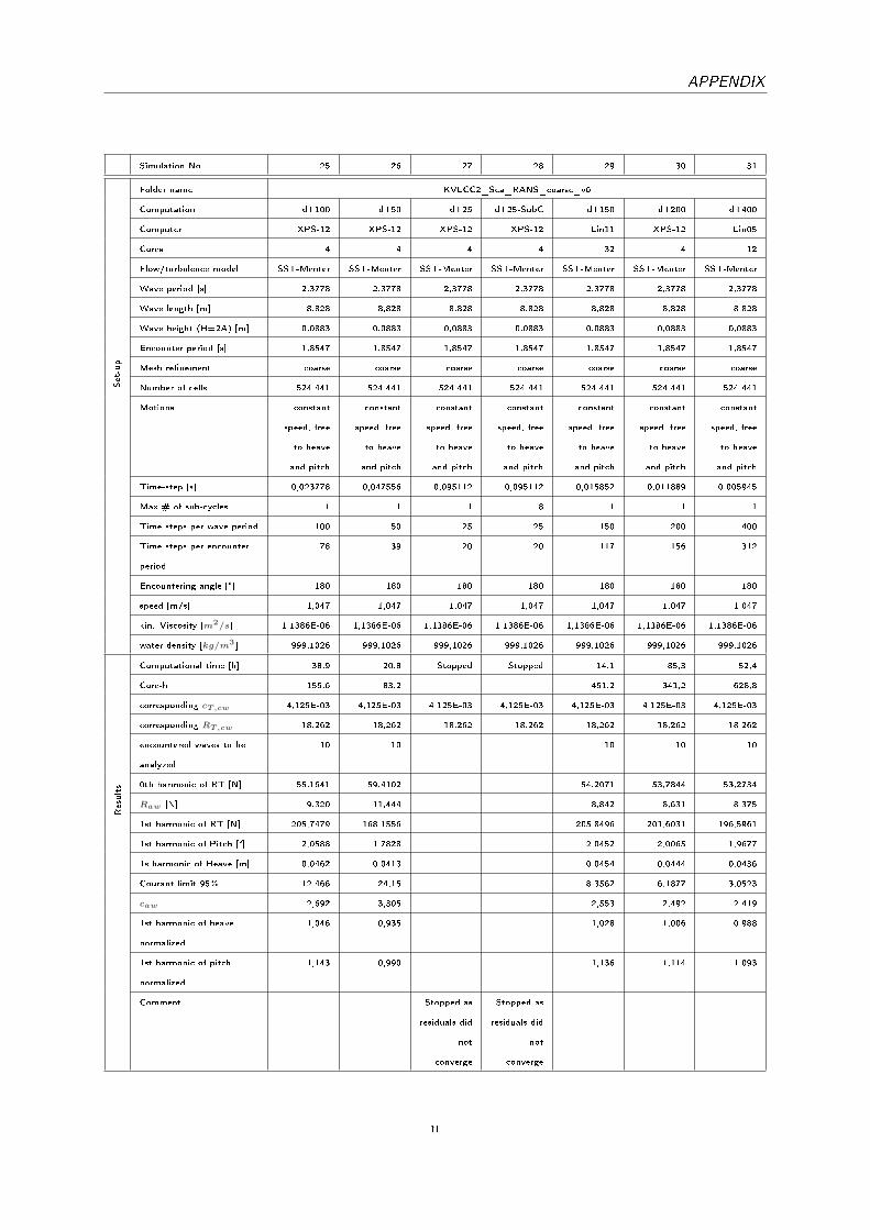
APPENDIX

Simulation No. 25 26 27 28 29 30 31

Set-up


Computation dT100 dT50 dT25 dT25-SubC dT150 dT200 dT400

Computer XPS-12 XPS-12 XPS-12 XPS-12 Lin11 XPS-12 Lin05

Cores 4 4 4 4 32 4 12

Flow/turbulence model SST-Menter SST-Menter SST-Menter SST-Menter SST-Menter SST-Menter SST-Menter

Wave period [s] 2,3778 2,3778 2,3778 2,3778 2,3778 2,3778 2,3778

Wave length [m] 8,828 8,828 8,828 8,828 8,828 8,828 8,828

Wave height (H=2A) [m] 0,0883 0,0883 0,0883 0,0883 0,0883 0,0883 0,0883


Mesh re�nement coarse coarse coarse coarse coarse coarse coarse

Number of cells 524.441 524.441 524.441 524.441 524.441 524.441 524.441

Motions constant

speed, free

to heave

and pitch

constant

speed, free

to heave

and pitch

constant

speed, free

to heave

and pitch

constant

speed, free

to heave

and pitch

constant

speed, free

to heave

and pitch

constant

speed, free

to heave

and pitch

constant

speed, free

to heave

and pitch

Time-step [s] 0,023778 0,047556 0,095112 0,095112 0,015852 0,011889 0,005945




period

78 39 20 20 117 156 312


speed [m/s] 1,047 1,047 1,047 1,047 1,047 1,047 1,047



Results

Computational time [h] 38,9 20,8 Stopped Stopped 14,1 85,3 52,4

Core-h 155,6 83,2 451,2 341,2 628,8




analyzed

10 10 10 10 10

0th harmonic of RT [N] 55,1641 59,4102 54,2071 53,7844 53,2734

Raw [N] 9,320 11,444 8,842 8,631 8,375

1st harmonic of RT [N] 205,7479 168,1556 205,8496 201,6031 196,5961

1st harmonic of Pitch [°] 2,0588 1,7828 2,0452 2,0065 1,9677

1s harmonic of Heave [m] 0,0462 0,0413 0,0454 0,0444 0,0436

Courant limit 95% 12,466 24,15 8,3562 6,1877 3,0523

caw 2,692 3,305 2,553 2,492 2,419


normalized

1,046 0,935 1,028 1,006 0,988


normalized

1,143 0,990 1,136 1,114 1,093

Comment Stopped as

residuals did

not

converge

Stopped as

residuals did

not

converge

n

APPENDIX

Simulation No. 32 33 34 35 36 37

Set-up

Folder name KVLCC2_Sea

_RANS

_coarse_v6

KVLCC2_Sea_RANS_medium_v3

Computation dT50Courant15 dT50 dT50-SubC dT100 dT200 dT400

Computer Lin11 Lin11 Lin11 Lin11 Lin11 Chalmers

Cores 32 32 32 32 32 32

Flow/turbulence model SST-Menter SST-Menter SST-Menter SST-Menter SST-Menter SST-Menter

Wave period [s] 2,3778 1,4561 1,4561 1,4561 1,4561 1,4561

Wave length [m] 8,828 3,310 3,310 3,310 3,310 3,310

Wave height (H=2A) [m] 0,0883 0,0662 0,0662 0,0662 0,0662 0,0662


Mesh re�nement coarse medium medium medium medium medium

Number of cells 524.441 4.860.201 4.860.201 4.860.201 4.860.201 4.860.201

Motions constant

speed, free

to heave

and pitch

constant

speed, free

to heave

and pitch

constant

speed, free

to heave

and pitch

constant

speed, free

to heave

and pitch

constant

speed, free

to heave

and pitch

constant

speed, free

to heave

and pitch

Time-step [s] 0,047556 0,029122 0,029122 0,014561 0,007281 0,00364




period

39 34 34 68 137 274


speed [m/s] 1,047 1,047 1,047 1,047 1,047 1,047



Results

Computational time [h] 4,3 stopped 85,3 35,2 158,1 168

Core-h 137,6 2729,6 1126,4 5059,2 5376




analyzed

10 10 10 10

0th harmonic of RT [N] 61,8609 46,6756 46,9386

Raw [N] 12,669 5,343 5,475

1st harmonic of RT [N] 176,8814 109,3658 121,4453

1st harmonic of Pitch [°] 1,8557 0,0693 0,0751

1s harmonic of Heave [m] 0,043 0,0015 0,0018

Courant limit 95% 17,227 38,825 19,006

caw 3,659 2,745 2,813


normalized

0,974 0,045 0,054


normalized

1,031 0,019 0,021

Comment Stopped, as

residuals did

not

converge

Residuals

did not

converge

Unable to

complete

simulation

o

APPENDIX

Simulation No. 38 39 40 41 42 43 44

Set-up

Folder name KVLCC2_Sea_RANS_medium_v4 KVLCC2_Sea_Euler_coarse_v3

Computation dT50 dT50-SubC dT100 dT200_2 dT400 dT100 dT200

Computer Lin11 Lin11 Lin11 Lin11 Lin11 XPS-12 XPS-12

Cores 32 32 32 32 32 4 4

Flow/turbulence model SST-Menter SST-Menter SST-Menter SST-Menter SST-Menter Euler Euler

Wave period [s] 2,3778 2,3778 2,3778 2,3778 2,3778 2,3778 2,3778

Wave length [m] 8,828 8,828 8,828 8,828 8,828 8,828 8,828

Wave height (H=2A) [m] 0,0883 0,0883 0,0883 0,0883 0,0883 0,0883 0,0883


Mesh re�nement medium medium medium medium medium coarse coarse

Number of cells 1.871.045 1.871.045 1.871.045 1.871.045 1.871.045 309.532 309.532

Motions constant

speed, free

to heave

and pitch

constant

speed, free

to heave

and pitch

constant

speed, free

to heave

and pitch

constant

speed, free

to heave

and pitch

constant

speed, free

to heave

and pitch

constant

speed, free

to heave

and pitch

constant

speed, free

to heave

and pitch

Time-step [s] 0,047556 0,047556 0,023778 0,011889 0,005945 0,023778 0,011889




period

39 39 78 156 312 78 156


speed [m/s] 1,047 1,047 1,047 1,047 1,047 1,047 1,047



Results

Computational time [h] 7,2 23,3 14,3 57,9 148,3 27,4 55,6

Core-h 230,4 745,6 457,6 1852,8 4745,6 109,6 222,4




analyzed

10 10 10 10 10 10 10

0th harmonic of RT [N] 66,9461 0,5922 70,7355 54,9501 53,2245 22,5844 21,866

Raw [N] 15,478 -17,699 17,373 9,480 8,617 8,152 7,793

1st harmonic of RT [N] 156,9996 169,0229 202,6984 215,9764 203,7374 211,4716 206,2632

1st harmonic of Pitch [°] 1,5829 2,1977 2,037 2,1468 2,0335 2,0241 1,9742

1s harmonic of Heave [m] 0,0351 0,0344 0,0465 0,0479 0,0446 0,0439 0,0421

Courant limit 95% 66,758 123,16 36,902 19,087 9,7132

caw 4,470 -5,111 5,017 2,738 2,489 2,354 2,251


normalized

0,795 0,779 1,053 1,085 1,010 0,994 0,954


normalized

0,879 1,221 1,131 1,192 1,129 1,124 1,096

Comment Residuals

not entirely

converged

Residuals

did not

converge

p

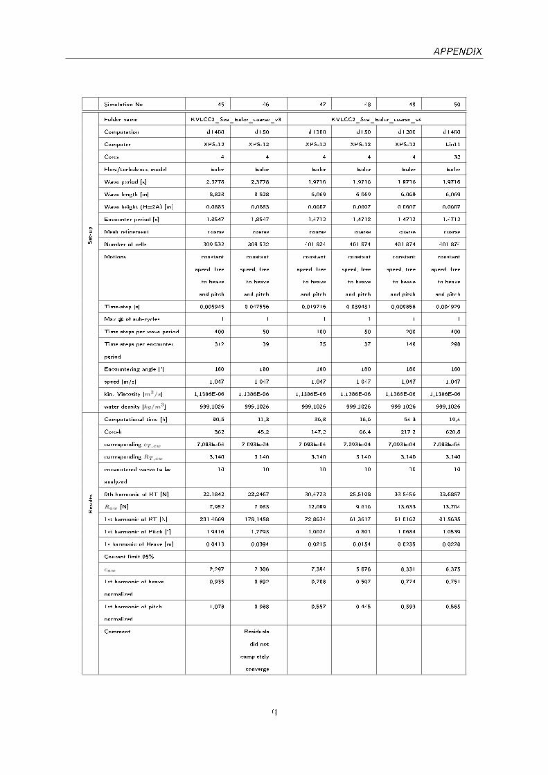
APPENDIX

Simulation No. 45 46 47 48 49 50

Set-up

Folder name KVLCC2_Sea_Euler_coarse_v3 KVLCC2_Sea_Euler_coarse_v4

Computation dT400 dT50 dT100 dT50 dT200 dT400

Computer XPS-12 XPS-12 XPS-12 XPS-12 XPS-12 Lin11

Cores 4 4 4 4 4 32

Flow/turbulence model Euler Euler Euler Euler Euler Euler

Wave period [s] 2,3778 2,3778 1,9716 1,9716 1,9716 1,9716

Wave length [m] 8,828 8,828 6,069 6,069 6,069 6,069

Wave height (H=2A) [m] 0,0883 0,0883 0,0607 0,0607 0,0607 0,0607


Mesh re�nement coarse coarse coarse coarse coarse coarse

Number of cells 309.532 309.532 401.874 401.874 401.874 401.874

Motions constant

speed, free

to heave

and pitch

constant

speed, free

to heave

and pitch

constant

speed, free

to heave

and pitch

constant

speed, free

to heave

and pitch

constant

speed, free

to heave

and pitch

constant

speed, free

to heave

and pitch

Time-step [s] 0,005945 0,047556 0,019716 0,039431 0,009858 0,004929




period

312 39 75 37 149 298


speed [m/s] 1,047 1,047 1,047 1,047 1,047 1,047



Results

Computational time [h] 90,5 11,3 36,8 16,6 54,3 19,4

Core-h 362 45,2 147,2 66,4 217,2 620,8




analyzed

10 10 10 10 10 10


Raw [N] 7,952 7,983 12,099 9,616 13,633 13,704




Courant limit 95%

caw 2,297 2,306 7,394 5,876 8,331 8,375


normalized

0,935 0,892 0,708 0,507 0,774 0,751


normalized

1,078 0,988 0,557 0,445 0,593 0,585

Comment Residuals

did not

completely

converge

q

APPENDIX

Simulation No. 51 52 53 54

Set-up

Folder name KVLCC2_Sea_Euler_coarse_v5

Computation dT100 dT200 dT400 dT50

Computer Lin11 Lin11 Lin11 Lin11

Cores 32 32 32 32

Flow/turbulence model Euler Euler Euler Euler

Wave period [s] 1,4561 1,4561 1,4561 1,4561

Wave length [m] 3,310 3,310 3,310 3,310

Wave height (H=2A) [m] 0,0662 0,0662 0,0662 0,0662

Encounter period [s] 0,9970 0,9970 0,9970 0,9970

Mesh re�nement coarse coarse coarse coarse

Number of cells 731.751 731.751 731.751 731.751

Motions constant

speed, free

to heave

and pitch

constant

speed, free

to heave

and pitch

constant

speed, free

to heave

and pitch

constant

speed, free

to heave

and pitch

Time-step [s] 0,014561 0,007281 0,00364 0,029122

Max # of sub-cycles 1 1 1 1

Time steps per wave period 100 200 400 50


period

68 137 274 34

Encountering angle [°] 180 180 180 180

speed [m/s] 1,047 1,047 1,047 1,047

kin. Viscosity [m2/s] 1,1386E-06 1,1386E-06 1,1386E-06 1,1386E-06

water density [kg/m3] 999,1026 999,1026 999,1026 999,1026

Results

Computational time [h] 7,9 19,43 43,5 4,5

Core-h 252,8 621,76 1392 144

corresponding cT,cw 7,093E-04 7,093E-04 7,093E-04 7,093E-04

corresponding RT,cw 3,140 3,140 3,140 3,140


analyzed

10 10 10 10

0th harmonic of RT [N] 15,7311 16,7342 16,8969 12,9346

Raw [N] 4,726 5,227 5,309 3,327

1st harmonic of RT [N] 117,3421 123,8059 124,6319 93,5463

1st harmonic of Pitch [°] 0,0727 0,0754 0,0758 0,0587

1s harmonic of Heave [m] 0,0018 0,002 0,002 0,0013

Courant limit 95%

caw 2,428 2,686 2,727 1,710


normalized

0,054 0,060 0,060 0,039


normalized

0,020 0,021 0,021 0,016

Comment Residuals

did not

converge in

the end of

the compu-

tation

Residuals

did not

always

converge

Residuals

did not

always

converge

r

APPENDIX

Simulation No. 55 56 57 58

Set-up

Folder name KVLCC2_Sea

_RANS

_oblique

_coarse_v5

KVLCC2_Sea

_RANS

_oblique

_coarse_v6

KVLCC2_Sea

_RANS

_oblique

_coarse_v7

KVLCC2_Sea

_RANS

_oblique

_coarse_v8

Computation dT150 dT150 dT150 dT150

Computer Lin11 Lin11 Lin11 Lin11

Cores 32 32 32 32

Flow/turbulence model SST-Menter SST-Menter SST-Menter SST-Menter

Wave period [s] 1,4561 1,9716 2,3778 1,8007

Wave length [m] 3,310 6,069 8,828 5,063

Wave height (H=2A) [m] 0,0662 0,0607 0,0883 0,1489

Encounter period [s] 1,0163 1,4941 1,8797 1,3339

Mesh re�nement coarse coarse coarse coarse

Number of cells 2.002.147 1.505.392 899.173 881.515

Motions constant

speed, free

to heave,

pitch and

roll

constant

speed, free

to heave,

pitch and

roll

constant

speed, free

to heave,

pitch and

roll

constant

speed, free

to heave,

pitch and

roll

Time-step [s] 0,009707 0,013144 0,015852 0,012005

Max # of sub-cycles 1 1 1 1

Time steps per wave period 150 150 150 150


period

105 114 119 111

Encountering angle [°] 160 160 160 160

speed [m/s] 1,047 1,047 1,047 1,047

kin. Viscosity [m2/s] 1,1386E-06 1,1386E-06 1,1386E-06 1,1386E-06

water density [kg/m3] 999,1026 999,1026 999,1026 999,1026

Results

Computational time [h] 60,35 53,2 36,1 35,4

Core-h 1931,2 1702,4 1155,2 1132,8

corresponding cT,cw 4,125E-03 4,125E-03 4,125E-03 4,125E-03

corresponding RT,cw 18,262 18,262 18,262 18,262


analyzed

10 10 10 8

0th harmonic of RT [N] 49,1927 63,2171 55,3945 137,0046

Raw [N] 6,335 13,347 9,436 50,241

1st harmonic of RT [N] 112,452 79,4612 228,7923 184,6681

1st harmonic of Pitch [°] 0,0499 1,0535 1,8069 1,7449

1s harmonic of Heave [m] 0,002 0,0251 0,044 0,0206

Courant limit 95% 12,52 8,3962 14,308 27,099

caw 3,255 8,157 2,725 5,102


normalized

0,060 0,827 0,997 0,277


normalized

0,014 0,585 1,004 0,330

Comment Oblique

waves

Oblique

waves

Oblique

waves

Oblique

waves

s

TRITA TRITA-SCI-GRU 2019:290

www.kth.se

efficient seakeeping performance predictions with...

Documents