460

POST PROCESSING TECHNIQUES STUDY FOR SEAKEEPING TESTS IN SHALLOW WATER

Marc Mansuy, Ghent University, Maritime Technology Division, Belgium

Manases Tello Ruiz, Ghent University, Maritime Technology Division, Belgium Guillaume Delefortrie, Flanders Hydraulics Research, Belgium

Marc Vantorre, Ghent University, Maritime Technology Division, Belgium

Despite the increased availability of numerical techniques, experimental analysis is still one of the most appropriate methods to study ship behaviour. For instance, the dynamics of a ship in waves are a complex problem ruled by several nonlinear phenomena, such as the free surface which can be hardly predicted, with sufficient accuracy, by any numerical method. Thus, the reliability of the measurements is not only of importance for a correct estimation of the ship behaviour but also to distinguish the phenomena involved. Post processing tools have been commonly applied to signal measurements to disregard noise and undesired effects. Fourier analysis, curve fitting, and averaging over time intervals are post processing tools frequently used. The present paper studies the suitability and limitations of such techniques when applied to study seakeeping model tests in shallow water. The experimental program has been conducted at Flanders Hydraulics Research (in cooperation with Ghent University) with a scale model of the DTC. Model tests comprise a variation of ship speeds, in head waves for two water depths.

1. Introduction

The ITTC provides practical guidelines to analyse regular wave tests at model scale in [1]. Three different post-processing methods are recommended to determine the fundamental period of the lead signal while amplitudes and phase angles are found using standard Fourier analysis on the response signals. However, due to facilities limitations (side-wall effect, waves reflection, transient effects, etc.) the post-processing of physical model tests in waves might be challenging. Some restrictions in shallow water tests have been studied at the Towing Tank for Manoeuvres in Shallow Water at Flanders Hydraulics Research ([2], [3] and [4]). To avoid these problems, tests with ship models in waves can be designed to obtain a specific time window characterised by:

• steady forward speed of the ship; • absence of reflections from the beach; • steady wave climate; • minimised tank side wall reflection.

However, the length of such time window can be limited and the minimum length of 10 cycles advised by the ITTC is sometimes not reachable (depending on the velocity and wave climate). Another alternative is the analysis of a longer time window and filtering out unwanted effects. In this case unexpected frequencies can be present in the measured signal, in addition to the fundamental frequency of the regular wave. Hence, post-processing analysis cannot be reduced to the identification of one single frequency signal. Moreover, in shallow water the wave profile becomes steeper and cannot be described properly by only one harmonic.

461

The influence of the sample length and analysing methods on the results is studied in section 4. The identification of time-dependant phenomena is illustrated in section 2 with a time-frequency analysis. In some cases, unexpected frequencies appear in between the wave’s harmonics, here a combination of low pass and stop band filters could be used. However, the cut off frequency selection is mostly unknown. Thus, filtering might not be necessary when the energy of the unwanted frequencies is not significantly high or when their frequencies can be differentiated from the ones of the harmonics under study. A selection of model tests executed at FHR is analysed using the different methods recommended by the ITTC in section 3.

2. Post-processing methods 2.1. Fast Fourier Transform The FFT is widely used because of its simplicity and fast computation time. However, one should bear in mind its restrictions and considerations. For instance, the Fast Fourier Transform assumes an infinite periodic signal, not achievable in reality, instead a truncated sample which do not consist of an integer number of periods is used, i.e. the infinite assumption is not fulfilled. Therefore the spectral analysis of the real signal can be biased showing energy spread around the true frequencies. The energy spread, called leakage, can be reduced by applying a window function on the signal before analysis. The window function will smooth the end points of the truncated signal to avoid discontinuity (the signal is then viewed as an infinite periodic repetition of the selected time window). However, the amplitude of the signal is weighted and a correction factor depending on the window’s type should be applied to estimate the true amplitude of the harmonics. Moreover, other restrictions when applying the FFT are related to the discretization of frequencies (sampling) which induces uncertainty in the frequencies identification (scalloping loss). This can be compensated by adding padding zeros to the signal. However, the resolution of the frequency (ability to find adjacent frequencies) is still limited by the size of the window (or sample length). The comparison of different types of window can be found in [6]. For example a flattop window will induce almost no scalloping loss. A rectangular window (or no window) will present a narrow main lobe, providing the best resolution of the peak frequency but difficulties to distinguish adjacent frequencies. The Hamming window is a good compromise for the present purpose. The accuracy of the peak frequency as well as the ability of distinguishing adjacent frequencies (frequency resolution) can be improved by increasing the window’s length. However, the length of the FFT is limited by processor’s capacity and the available length of the sample. In the next sections, the amplitude abof each harmonic is defined by ab =

|dd](b)|

6 with N the

number of sample points. If a window function is applied to the signal, a correction factor is used depending on the window’s type (see [6]). The maximum height ghNiis taken as the difference between the maximum and minimum values of the analysed signal. In the next section the FFT is computed without window (referred to as method 1) and with a Hamming window (referred to as method 2). In the present study 65000 points have been used by adding leading zeros.

462

2.2. Fitting method If the measured quantities can be modelled by a function f, the signal can also be directly fitted using a non-linear least square method. In the next sections, the function f is given by a Fourier series up to the third order is considered:

j kb, mb, n = ko + [kb cos tnbu + mbvw&(tnbu)

x

byB

] (1)

The mean value is given by ko, the fundamental frequency is given by nBand the amplitude of the

harmonics by ab = kb² + mb². The maximum height ghNi is the difference between the maximum

and minimum values of the fitted function. In the next sections this method is referred to as method 3. 2.3. Average on cycles The average of the period and amplitude of each wave cycle is taken over a selection of integer number of cycles. The mean value ko is the average of the amplitude computed for each cycle. The amplitude of the first harmonic aB is estimated by taking the standard deviation over the full length of the signal multiplied by 2. The maximum height ghNi is the average difference between the maximum and minimum values of each cycle. This method is referred to as method 4. 2.4. Selection of interval to be analysed The interval is determined manually by checking the time series according to the ITTC. The length of the analysed sample is therefore limited to a short steady and undisturbed part of the complete test. Once a time window has been defined, the length of the analysed signal is also restricted by the post-processing method which will be used. The method consisting of averaging a number of cycles requires integer number of cycles. Therefore, start and end points need to be defined, hence reducing the length of the signal. With a Fourier analysis, the beginning and the end of the signal is attenuated by the application of a window function. With the fitting method, no restriction is apparently needed. The effect of such restrictions is illustrated in the next sections by comparing the different post-processing methods mentioned above and applied on experimental tests. 3. Experimental program The experiments were conducted with the DTC container ship at the Towing Tank for Manoeuvres in Shallow Water at Flanders Hydraulics Research (FHR) in Antwerp, Belgium (in cooperation with Ghent University) in the framework of the European SHOPERA project. The towing tank main characteristics can be found in detail in [5] and [7]. During the tests, horizontal forces were measured by the load cells LC1 and LC2, the ship’s heave, pitch and roll motions were obtained by using four potentiometers P1 to P4 (see Fig. 1a). Wave profiles were recorded with four wave gauges, WG1 to WG3 located at a fixed position along the tank and WG4 attached to the main carriage (see Fig. 1b). Positions and orientations during the test are defined by using

463

two axes systems, an Earth-bound |o}o~o�o and a body-bound |}~�, both, North-East-Down oriented, see Fig. 1b. The tests taken as examples in this paper are described in Table 2.

Fig. 1 – Towing tank at FHR, set-up for semi captive tests for the DTC ship

The ship model’s main parameters for the DTC are given in Table 1.

Table 1 – Container ship model’s main parameters

Ship Lpp (m)

B (m)

Tdesign (m) Cb m

(kg) xG (m) zG (m) Ixx (kgm²)

Iyy (kgm²)

Izz (kgm²)

DTC 3.984 0.572 0.163 0.661 242.8 -0.052 -0.059 12 221 230

Table 2 – Experimental and numerical parameters for model tests in waves Ship speed Environment

Test ID Model scale [m/s]

Full scale [kts]

ukc [%]

Theoretical wave length

[m] Theoretical

wave frequency

[Hz]

Theoretical wave

frequency of

encounter [Hz]

Desired wave

amplitude [mm]

Wave encounter angle[°]

C2 0.872 16 100 - - - - - CW1 0 0 100 2.19 0.723 0.723 22.4 180 CW3 0.872 16 100 2.19 0.723 1.12 22.4 180 CW4 0 0 20 2.19 0.601 0.601 22.4 180

4. Experimental analysis and discussion 4.1. Time-frequency analysis The spectrogram provides a clear representation of the energy distribution in the time-space domain. It gives a good overview of the tests to select the optimum time window for the analysis. However a compromise needs to be found between high frequency resolution and time resolution.

0.258 m

-1.037 m

1) Potentiometer (P1-P4) 2) Load cell (LC1, LC2) 3) Pitch and roll mechanism 4) Vertical guidance

P2

c)

P1

0.258 m

-1.143 m

P3LC2

b)

LC1

a)0.987 m

1.137 m

P4

24

3

21 14

WA

VE MAK

ER

MA

IN C

AR

RIA

GE

0

y =2.6 m

y =3.5 m

h=180°

0y =2.6 m

m= h+ y

0

0.65 m

0

d

y

0o v0

y

xu

0

0

V

x

4.03 mHARBOUR

x =73.0 m

m

y =0 m0bY

0 0

o

x = 44.0 m x =+66.3 m

h

WG4

r

x = 24.0 m0

( l ,z )

0

WG3

y

0

WG2

Y

V

o

o

y x

x

WG1

x

464

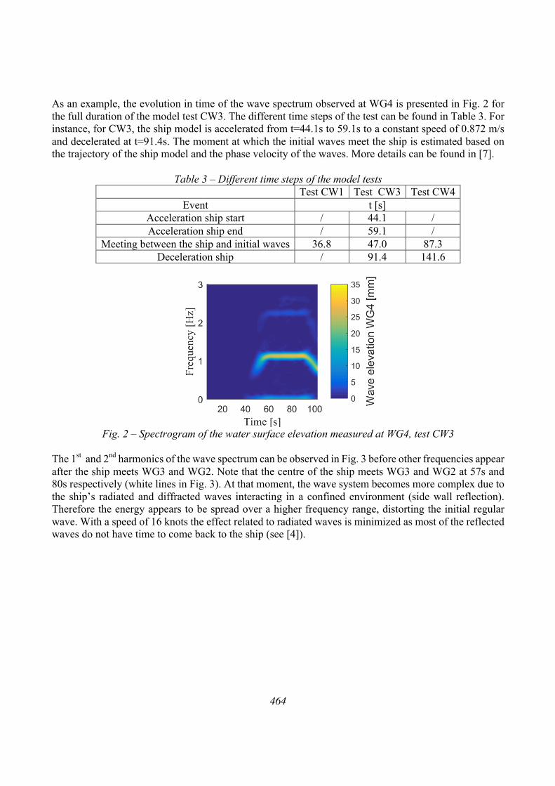
As an example, the evolution in time of the wave spectrum observed at WG4 is presented in Fig. 2 for the full duration of the model test CW3. The different time steps of the test can be found in Table 3. For instance, for CW3, the ship model is accelerated from t=44.1s to 59.1s to a constant speed of 0.872 m/s and decelerated at t=91.4s. The moment at which the initial waves meet the ship is estimated based on the trajectory of the ship model and the phase velocity of the waves. More details can be found in [7].

Table 3 – Different time steps of the model tests Test CW1 Test CW3 Test CW4

Event t [s] Acceleration ship start / 44.1 / Acceleration ship end / 59.1 /

Meeting between the ship and initial waves 36.8 47.0 87.3 Deceleration ship / 91.4 141.6

Fig. 2 – Spectrogram of the water surface elevation measured at WG4, test CW3

The 1st and 2nd harmonics of the wave spectrum can be observed in Fig. 3 before other frequencies appear after the ship meets WG3 and WG2. Note that the centre of the ship meets WG3 and WG2 at 57s and 80s respectively (white lines in Fig. 3). At that moment, the wave system becomes more complex due to the ship’s radiated and diffracted waves interacting in a confined environment (side wall reflection). Therefore the energy appears to be spread over a higher frequency range, distorting the initial regular wave. With a speed of 16 knots the effect related to radiated waves is minimized as most of the reflected waves do not have time to come back to the ship (see [4]).

465

Fig. 3 – Spectrogram of the water surface elevation measured at WG3 and WG2; the moment in time at

which the ship is passing in front of the gauge is indicated with a white line, test CW3.

Other phenomena can be identified on these graphs such as noise around 5 Hz visible in the measurement of the longitudinal force or unexpected response at 1.66 Hz (Fig. 4). Note that the latter may be noise induced by wave gauges as it is observed in both calm water and waves. Once such phenomenon has been identified, it seems natural trying to remove those frequencies from the response signal. A spectral analysis (FFT) applied on a steady part of the signal provides more accurate information about the bandwidths to be removed (Fig 5). Note that the frequency resolution (defined in [6]) is limited by the window’s type and sample length (see Fig. 6). This is not an issue as long as it does not hide any adjacent frequency.

Fig. 4 – Spectrogram of the total longitudinal force X in calm water test C2 (left) and waves test CW3

(right), 1.66Hz response visualized in black frame.

466

Fig. 5 – Amplitude spectrum X force and water surface elevation at WG4

Fig. 6 – Frequency resolution FFT defined by eq. 2 and eq. 3

jÄÅO_ÉNhhQÑM = 1.81 dO

6 (2)

jÄÅO_`ÅÜáNÑMSPNÄ = 1.21 dO

6 (3)

4.2. Comparison of four methods to find the fundamental frequency The options recommended by the ITTC to find the fundamental frequency have been applied to the measurement of the water surface elevation measured at WG2 and WG4. The four methods are described in section 2. Each method has been applied on the full time series and a selection of wave cycles for the test presented in section 3. Note that in this section a detrend function is used to remove the mean value. It can be noticed that the average method (method 4) is more sensitive to the number of cycles while the other methods converge to a single value (Fig. 7). With a few number of cycles, the frequency obtained with the hamming window differs significantly because of the low frequency resolution. The resolution of the rectangular window is better and the frequencies obtained with low number of cycles are closer to the value obtained for the full sample length (Fig 6 and Fig 7). The fitting method is less sensitive to the number of cycles. Its reliability of the parameter’s estimation is also improved by increasing the record’s length or analysing several time records of equal length [8].

0

0.5

1

1.5

2

2.5

0 5 10 15 20

Freq

uenc

y re

solut

ion

[Hz]

Number of cycles [-]

Hamming windowRectangular window

467

The fundamental frequency computed on the maximum sample length (steady forward speed of the ship) is shown in Table 3 for the wave profiles as measured in WG2 and WG4. From all the methods, the average method seems to be more sensitive to noise.

Fig. 7 – Fundamental frequency computed with different post-processing methods and different sample

lengths at WG2 (left) and WG4 (right).

Table 3 – Fundamental frequency and frequency of encounter

Method n°1

Method n°2

Method n°3

Method n°4

WG2 0.724 0.724 0.724 0.725 WG4 1.122 1.122 1.122 1.061

4.4. Comparison of four methods to compute forces amplitudes The previous methods have been used to estimate the gain of each harmonic as well as the maximum height of the longitudinal force for the full sample length. The ITTC recommends to use a Fourier analysis constraining the fundamental frequency to the value computed from the lead signal in 4.1 but this constraint does not show significant effect (Table 4).

Table 4 – Longitudinal force characteristics computed with fitting Fourier Series (3rd order) Unconstrained frequency Constrained frequency

ko [N] 7.34 7.36 ghNi [N] 17.92 17.88 jB [Hz] 1.12 1.12 aB[N] 8.58 8.56 j' [Hz] 2.25 2.24 a' [N] 0.98 0.99

468

The amplitudes obtained with the different post-processing methods are shown in Fig. 8 for the full sample length of the different tests described in section 3. It can be noticed that ghNi and ko are sensitive to the selected method. For instance, at zero speed and 100% ukc (test CW1), ko is 26% lower with method 4 than method 3. The influence of the window applied before the FFT is slightly visible with the test CW1 for which ko is 15% lower without windowing. However the added resistance obtained with test CW3 varies only from 10 to 12% depending on the methods. In general the estimates from the fitting method are close to the FFT except for ghNi which differs by up to 10N with test CW3.

Fig. 8 – Longitudinal force measured during tests CW1 (a), CW3 and C2 (b), CW4 (c).

The discrepancies between the different methods increased when the sample length is reduced (Fig. 9).

0.0

0.2

0.4

0.6

0.8

1.0

02468

10121416

1 2 3 4

!0 [N

]

X fo

rce

[N]

Post-processing method [N°]

a)

0.0

2.0

4.0

6.0

8.0

10.0

02468

10121416

1 2 3 4

!0 [N

]

X fo

rce

[N]

Post-processing method [N°]

0.0

0.2

0.4

0.6

0.8

1.0

02468

10121416

1 2 3 4

!0 [N

]

X fo

rce

[N]

Post-processing method [N°]

c)0.00

5.00

10.00

15.00

20.00

25.00

30.00

1 2 3 4

Longitu

dinalforce[N

]

Post-processingmethod[N°]

calm water a0Hmax/2 G1G2 G3

469

Fig. 9 – Longitudinal force measured for different sample lengths during tests CW3.

4.5. Comparison of four methods to compute motion amplitudes The variations of motion amplitudes between the different methods is also significant. For instance, the trim (ko) differs by 0.2 mm/m between method 1 and 4 during the test CW1 and ghNi varies within 1 mm (Fig. 11). The mean sinkage (ko) is found to be increased by 7 to 9% in waves compared to calm water depending on the methods (Fig. 11).

0.0

0.2

0.4

0.6

0.8

1.0

0123456

1 2 3 4

!0 [m

m/m

]

Pitc

h [m

m/m

]

Post-processing method [N°]

a)

0.0

0.2

0.4

0.6

0.8

1.0

0123456

1 2 3 4

!0 [m

m/m

]

Pitc

h [m

m/m

]

Post-processing method [N°]

b)

0.0

0.2

0.4

0.6

0.8

1.0

0123456

1 2 3 4

!0 [m

m/m

]

Pitc

h [m

m/m

]

Post-processing method [N°]

c) 0.001.002.003.004.005.006.007.008.009.0010.00

1 2 3 4

Longitu

dinalforce[N

]

Post-processingmethod[N°]

calm water a0Hmax G1G2 G3

470

Fig. 10 – Pitch motion measured during tests CW1 (a), CW3 and C2 (b), CW4 (c).

Fig. 11 – Heave motion measured during tests CW1 (a), CW3 and C2 (b), CW4 (c).

5. Discussion about filtering The quality of the signal can be improved by filtering unwanted frequencies. Fig 12 and Fig 13 show the effect of filtering the frequency around 5Hz (identified as noise in the measured forces) and 1.66Hz (identified in 3.1) on the longitudinal force measured during CW3 as an example. A Lanczos stopband filter has been applied in the frequency domain for simplicity to remove the frequency at 1.66Hz. The parameters of the filter are adjusted to achieve zero response at the band centre (see [9]). A Lanczos low pass filter has been used to remove the noise around 5Hz. The discrepancy between the post-processing methods observed for ghNi and ko is reduced after filtering. Moreover, it is clear that without filtering the definition of one period using zero-crossing detection is more challenging (Fig 12). Note that because the filters are applied in the frequency domain, the bandwidth is limited by the sample length. This can be a problem when trying to remove frequencies very close to another peak frequency. Indeed, as the resolution of the FFT (i.e. sample length) defines the ability to find adjacent frequencies, it is also a limit for removing adjacent frequencies.

0.00.10.20.30.40.50.60.70.80.9

012345678

1 2 3 4

!0 [m

m]

Hea

ve [

mm

]

Post-processing method [N°]

a)

6.36.46.56.66.76.86.97.07.17.2

012345678

1 2 3 4

!0 [m

m]

Hea

ve [

mm

]

Post-processing method [N°]

b)

0.00.10.20.30.40.50.60.70.8

012345678

1 2 3 4

!0 [m

m]

Hea

ve [

mm

]

Post-processing method [N°]

c) 0.001.002.003.004.005.006.007.008.009.0010.00

1 2 3 4Longitu

dinalforce[N

]Post-processingmethod[N°]

calm water a0Hmax G1G2 G3

471

Fig. 12 – Effect of filtering on the time series of the X force measured during CW3.

Fig. 13 – Effect of filtering on the longitudinal force measured during CW3, before filtering(left) and

after filtering (right).

6. Conclusion The analysis of towing tank tests in shallow and confined water may be challenging due to facilities limitations but simple post-processing methods (FFT, function fitting, average) may still be considered for the analysis of short time series in regular waves. The spectrogram is useful for visualisation of different phenomenon occurring during a ship model test. As linear theory is assumed, unexpected frequencies can then be identified and filtered to remove unwanted distortion of the response signal for which an averaging method can be for instance very sensitive. However, the cut off bandwidth is sometimes not well identified and the selection of filtering settings might be challenging. To avoid the use of complex filters, FFT or fitting functions seem suitable for the analysis of seakeeping tests in shallow water as long as the length of the sample is long enough so that the frequencies of such phenomenon can be distinguished from the peak frequencies. Interesting further research is to identify more thoroughly the sources of unwanted frequencies in a confined towing tank (side-walls, wake, noise in instrumentation…) to be able to separate such

0.0

2.0

4.0

6.0

8.0

10.0

02468

10121416

1 2 3 4

!0 [N

]

Long

itudi

nal

forc

e [N

]

Post-processing method [N°]

0.0

2.0

4.0

6.0

8.0

10.0

02468

10121416

1 2 3 4

!0 [N

]

X fo

rce

[N]

Post-processing method [N°]0.00

10.00

20.00

30.00

40.00

50.00

60.00

70.00

1 2 3 4

Longitu

dinalforce[N

]

Post-processingmethod[N°]

calm water a0 Hmax G1 G2 G3

472

frequencies from peak frequencies when they are of similar energy. Moreover, pre-processing methods could be directly applied in real time to avoid disturbing the response signal during the test record. 7. Acknowledgements The research described in this paper is performed in the frame of project WL_2013_47 (Scientific support for investigating the manoeuvring behaviour of ships in waves), granted to Ghent University by Flanders Hydraulics Research, Antwerp (Flemish Government). The model tests were performed within the project SHOPERA - Energy Efficient Safe SHip OPERAtion, which was partially funded by the EU under contract 605221. 8. Nomenclature a0 [mm] Mean Fourier series ai [mm] ith order cosine terms Fourier series B [m] Breadth of the ship bi [mm] ith order sine terms Fourier series CB [-] Block coefficient Fs [Hz] Sample frequency GMT [m] Transverse metacentric height Ixx [kg m²] Mass moment of inertia about Ox-axis Iyy [kg m²] Mass moment of inertia about Oy-axis Izz [kg m²] Mass moment of inertia about Oz-axis Lpp [m] Length between perpendiculars m [kg] Mass N [-] Number of sample points O [-] Origin of the ship-bound axis system O0 [-] Origin of the earth-bound axis system O0x0,y0,z0 [-] Earth bound coordinate system Ox,y,z [-] Ship bound reference system Tdesign [m] Design draft u [m/s] Longitudinal ship velocity ukc [%] Under keel clearance v [m/s] Lateral ship velocity V [m/s] Ship velocity xg [m] Centre of gravity (longitudinal) X [N] Longitudinal force zg [m] Centre of gravity (vertical) δ [°] Rudder angle η [°] Wave angle λ [m] Wave length µ [°] Wave encounter angle ψ [°] Ship’s heading ω [rad/s] Wave frequency C2 Captive calm water model tests 2 CM Clamping mechanism

473

CW1-4 Captive wave model tests 1-4 P1-4 Potentiometers 1-4 DTC Duisburg Test Case FHR Flanders Hydraulics Research LC1-2 Load cells 1-2 R1-4 Reflector plates 1-4 H1-2 Height meters 1-2 MASHCON Manoeuvring in shallow and confined water S1-4 Lasers 1-4 SHOPERA Ship operation WG1-4 Wave gauges 1-4 FFT Fast Fourier Transform 8. References 1. ITTC, (2014), “ITTC – Recommended Procedures and Guidelines - Seakeeping Experiments”,

7.5-02-07-02.1 (Revision 04). ITTC: pp. 1-22. 2. Tello Ruiz, M., De Caluwé, S., Van Zwijnsvoorde, T., Delefortrie, G., Vantorre, M., (2015),

“Wave effects in 6DOF on a ship in shallow water”, MARSIM 2015. Newcastle upon Tyne, UK. Newcastle University: Paper 2.2.2, pp. 1-15.

3. Tello Ruiz, M., Vantorre, M., Van Zwijnsvoorde, T., Delefortrie, G., (2016), “Challenges with ship model tests in shallow water”, Proceedings of The 12th International Conference on Hydrodynamics, ICHD2016, Egmond aan Zee, The Netherlands. TU Delft, Paper 59: pp. 1-10.

4. Tello Ruiz, M., Van Hoydonck, W., Delefortrie, G., Vantorre, M., (2017), “On the limitations of ship model tests in waves in a shallow water and narrow towing tank”, Submitted to the 20th Numerical Towing Tank Symposium (NuTTS 2017), Wageningen, The Netherlands.

5. Delefortrie, G., Geerts, S., Vantorre, M., (2016), “The Towing Tank for Manoeuvres in Shallow Water”, 4th MASHCON International Conference on Ship Manoeuvring in Shallow and Confined Water with Special Focus on Ship Bottom Interaction, Hamburg, Germany, BAW: pp. 226-235. DOI: 10.18451/978-3-939230-38-0_27.

6. Frederic J. Harris, (1978), “On the Use of Windows for Harmonic Analysis with the Discrete Fourier Transform”, Proceedings of the IEE, Vol. 66 No. 1.

7. Van Zwijnsvoorde, T., Delefortrie, G., Lataire, E., (2019), “Sailing in shallow water waves with the DTC container carrier: open model test data for validation purposes”, 5th MASHCON International Conference on Ship Manoeuvring in Shallow and Confined Water, 20-22 May, 2019, Ostend, Belgium

8. D. Brook, R. J. Wynne, (1988), “Signal Processing – Principles and Applications”, Edward Arnold, pp. 181-216.

9. Claude E. Duchon, (1979), “Lanczos Filtering in One and Two Dimensions”, School of Meteorology, University of Oklahoma, Norman 73019