IEEE TRANSACTIONS ON MICROWAVE THEORY AND TECHNIQUES, VOL. 42, NO. 1, JANUARY 1994 99

Efficient Mode Analysis with Edge Elements and 3-D Adaptive Refinement

Nikolaos A. Golias, Antonis G. Papagiannakis, and Theodoros D. Tsiboukis

Abstract- Efficient mode analysis of 3-D inhomogeneously loaded cavity resonators of arbitrary shape by the finite edge el- ement method is presented in this paper. Two weak formulations involving field vectors E and H are derived from a Galerkin weighted scheme resulting in a sparse symmetric generalized eigenvalue problem, the solution of which is obtained by a sparse eigenvalue technique. Edge elements with divergence free shape functions guarantee the continuity of the tangential components of the field variables E or H, but not of their normal components, across element interfaces in contrast with node based elements that impose full continuity. The discontinuity of the normal component of D or B, present in the numerical model, is proposed as an error estimator suitable for adaptive mesh refinement of 3-D tetrahedral meshes with edge elements. Application to a dielectrically loaded cavity is given with full documentation and by way of illustration.

I. INTRODUCTION HE solution of high-frequency 3-dimensional electromag- T netic field problems encounters some difficulties asso-

ciated with the simultaneous satisfaction of the Maxwell’s equations. This is reflected in the many formulations developed for their solution [ 13-[ 141. For the solution of high-frequency 3-dimensional problems in a current and charge free space, two dual formulations are well known-one with the magnetic intensity A and one with the electric intensity E. When attempting to solve for the fields E or H with conventional node based elements, it is found that unwanted “spurious” solutions appear, possibly due to the “overcontinuity” that these elements impose on the electromagnetic fields, that do not satisfy the zero divergence condition of the magnetic flux density V B = 0 or of the electric flux density V D = 0.

The basis of the problem originates directly from “Maxwell’s equations” and the nature of the electromagnetic fields. Since the field variables E or A must satisfy two equations, the vector wave equation and the zero divergence condition, a simultaneous solution is requested to give the desired fields. But the simultaneous solution of these equations is at least very difficult for the general case of 3-D domains. Solution of the vector wave equation must be accomplished in such a way that the zero divergence condition holds in a mean weighted sense. In addition, E or E must fulfill certain boundary conditions across interfaces between different material regions, and that is continuity of the tangential but not of the normal components.

Manuscript received July 30, 1992; revised February 22, 1993. The authors are with the Department of Electrical Engineering, Aristotle

IEEE Log Number 9213729. University of Thessaloniki, Thessaloniki, 54006 Greece.

Several formulations have been proposed in order to remove these unwanted solutions: a common practice is to impose the zero divergence condition in an average sense by introducing a penalty term in the variational procedure [4], [6], [lo]. Although this approach does not eliminate completely spurious modes, it pushes the associated eigenvalues higher in the spectrum, i.e., out of the region of practical interest. l b o other methods which have been proposed employ divergence free fields [5 ] , [7], or introduce a new relationship between the field variables via a connection matrix [2], [3].

Node elements were used in the above approaches that impose full continuity of the field variables E or H, that is, overcontinuity across material interfaces. Another kind of element, the so-called “edge” element, seems to possess the right continuity conditions for the fields E or H , that is, tangential continuity, and have been used satisfactorily for the solution of E-M field problems [ 151, [ 181, [ 191. In edge elements, the basis functions are associated with the edges of the mesh and impose continuity for the tangential components of the fields E or H , but not of their normal components, so they do not impose overcontinuity as is the case with node elements. This is in accordance with the exact solution that requires E or H to have tangential continuity, but not normal continuity at material interfaces. A result of this is that no spurious modes are present in eigenvalue problems handled with edge elements, as is explained very extensively and from a mathematical point of view in [16].

The exact solution requires continuity of the normal compo- nents of D or B. The edge element approximation functions do not impose such a continuity, and in fact the normal components of the numerical approximation are discontinuous. This discontinuity of the normal components is suggested as an error estimator, suitable for adaptive mesh refinement.

There are many advantages of using an automatic-adaptive mesh generator [20]. The optimal solution is obtained with the minimum computational cost, since degrees of freedom are inserted in regions of high error. The process is completely automatic, so that a minimum of data is needed as input in such an expert system, and analysis follows without user intervention. It must be pointed out that the reduction of the computational cost is a very important parameter since it can be very high, especially in the solution of eigenproblems as is the case with the analysis of resonant cavities.

A previous implementation of the 3-D adaptive mesh gen- eration procedure with node elements has shown excellent results 1201. In this paper, an extension is attempted to vectorial edge-based elements. High error regions, i.e., regions that

0018-9480/94$04.00 0 1994 IEEE

100 IEEE TRANSACTIONS ON MICROWAVE THEORY ANI) TECHNIQUES, VOL. 42, NO. 1, JANUARY 1994

present the highest error in the approximation procedure, are identified and refined completely automatically. Hence, new degrees of freedom, edges in our case, are inserted in those regions so that the error in the approximation procedure is minimized.

In the following, we first present the basic field equations of high-frequency problems and their weak formulations, followed by a section describing the finite element formulation with edge elements. Then a discussion about the nature of sym- metry planes and the exploitation of symmetry is presented. In Sections VI and VII, we describe the newly proposed criterion of error estimation and the implementation of the self-adaptive automatic mesh refinement procedure. Finally, application to a problem of a dielectrically loaded cavity, for which results with other implementations exist in the literature, is given to show the efficiency and robustness of the proposed self- adaptive refinement scheme. Differences between these results and those from other implementations, possibly due to the use of improper symmetry planes, is discussed in Section VII.

11. THE FIELD EQUATIONS

Consider the case of a current and charge free space 0 with boundary dR, filled with inhomogeneous and possibly anisotropic material. Then the Maxwell’s equations become

a B V X E = - - at

dD V X H = - at together with the constitutive relations

B = [PIH D = [~Iepsilon

(3)

(4)

where E is the electric field intensity, H is the magnetic field intensity, B is the magnetic flux density, D is the electric flux density, [ p ] is the magnetic permeability tensor, and [ E ] is the electric permittivity tensor of the medium.

Assuming harmonic variation with time, (3) and (4) become

(7) V x E = - j ~ [ p ] H

V x H = j w [ ~ ] E . (8)

Without any loss in generality, we consider nonmagnetic materials. From the combination of the above equations, we get the following vector wave equation for E and H which the modes in the cavity must satisfy

(9) v x (V x E ) - k,2[E,]E = 0

v x ( [ E p V x H ) - k:H = 0 (10)

with k,” = w 2 p L , ~ , being the square of the wavenumber, and [ E , ] the relative permittivity tensor.

The boundary conditions for the electric field intensity E require the vanishing of the tangential components of the electric intensity on perfect electric conductors (n x E = 0 ) (E normal to the wall) and the vanishing of the tangential components of H (n x (V x E ) = 0) ( H normal to the wall) on perfect magnetic conductors. The boundary conditions for the H case require the vanishing of the tangential components of the magnetic field intensity on perfect magnetic conductors (n x H = 0 ) and the vanishing of the tangential components of the electric field vector (n x ( [ E ] - ~ V x H ) = 0) on perfect electric conductors.

111. WEAK FORMULATION

In order to approximate the vector wave equations (9) or (10) with a numerical scheme, their weak forms are consid- ered. By weighting (9) with a suitable weighting function E’, we obtain the following weak formulation for E:

L V x (V x E ) .E’dv - IC: [~, lE.E’dw = 0 (11) s, which is transformed using the first vector Green’s identity as

L ( V x E ) . (V x E’)dv - IC:

[E’ x (V x E ) ] .rids = 0. (12) d n

Similarly, by weighting (10) with a suitable weighting function H’, the following weak formulation for H is obtained:

which is transformed by the first vector Green’s identity as

/ ( [ ~ , ] - ‘ v x H ) - ( V x n H‘)dv -k :

[H’ x ([E,]-’V x H ) ] .rids = 0. (14) -/an

Boundary conditions for the E formulation are homoge- neous Dirichlet type on perfect electric conductors (short circuits) and homogeneous Neumann on perfect magnetic con- ductors (open circuits). In the same way, boundary conditions for the H formulation are homogeneous Dirichlet on perfect magnetic conductors and homogeneous Neumann on perfect electric conductors. In either case, the tangential part in (12) and (14) does not contribute, and thus only volume integrals remain in the final equations.

IV. FORMULATION WITH EDGE ELEMENTS

Tetrahedral elements with unknowns prescribed on the edges [ 151, [ 181 are used here for the discretization of the weak Galerkin forms (12) and (14) of the vector wave equations. The basis functions for the first-order 1-form Whitney tetrahedral elements for a typical edge e = {i, j } connecting vertices i and j are given by

GOLIAS et al.: EFLlCIENT MODE ANALYSIS WlTH EDGE ELEMENTS 101

where Ci (i = 1, 2, 3, 4) are the simplex or local coordinates of the tetrahedron.

The interpolated field is given by 6

F = CFiWi (16) i=l

where the coefficients Fi are the circulations of the field intensity along the edges of the tetrahedron. -0 easily obtained properties are the continuity of tangential components across elements interfaces and zero divergence [ 151.

If the vector weighting functions in (12) and (14) are chosen to be the vector shape functions of the edge elements, then the following generalized eigenvalue problem is obtained:

[AI[Xl = W [ X I (17)

where [A] and [B] are matrices with elements

aij = J,(v x W i ) . ( V x Wj )dv (18)

b;j = [E, ]W~ * W j dv (19) J,

J , J

for the E formulation and

aij = L ( [ E ~ ] - ' V x W i ) . (V x W j ) dv (20)

bij = Wi * W - dv (21)

for the H formulation. Solution of the generalized eigenvalue problem (17) is

obtained by inverse iteration with shifting implemented in conjunction with the ICCG method of solving a system of linear equations, fully exploiting sparsity and symmetry of the finite element matrices, resulting in very fast convergence.

V. EXPLOITING SYMMETRY In many situations, the geometry of the problem domain is

such that a great reduction in computations can be achieved by the introduction of symmetry planes. In many cases, a fraction of the geometry such as one-half, one-fourth, etc., can be considered with the associated reduction in cost [17]. Special attenuation must be taken with the introduction of symmetry planes, so that they correspond to the nature of the electromagnetic fields. For the case of a lossless resonant cavity, we have seen that boundary conditions correspond either to an electric conducting wall (short-circuit) or to a magnetic conducting wall (open circuit).

An electric conducting wall corresponds to a short circuit, and the boundary conditions there are homogeneous Dirichlet since the circulation of E on this wall is zero. Analogously, a magnetic conducting wall corresponds to an open circuit, and the boundary conditions there are homogeneous Neumann for the field H.

Consider, for example, the case of a cubic resonator excited with two modes, as is shown in Fig. l(a) and (b), where the lines of H are shown. It is clear that the symmetry plane introduced in Fig. l(a) is a magnetic wall (A normal to

Magnetk conducting Wall

I

I Elect& conducting Wall

Fig. 1. Symmetry planes.

the wall); while in Fig. l(b), an electric conducting wall ( H tangential to the wall). The nature of the symmetry planes then corresponds to the mode present in the cavity and must be taken into consideration.

VI. ERROR ESTIMATION

Edge-based basis functions as presented in Section IV assure the continuity of the tangential components of the field intensity across element interfaces, but not of their normal components. This is in accordance with the fact that in exact solutions, the fields E or H have continuous tangential components, but may have discontinuous normal components across interfaces between different media. In fact, the constitutive fields D or B must have continuous normal components. Edge Elements do not impose such a continuity of the normal components of D or B, allowing these normals to be discontinuous across element interfaces. This is an indi- cation that this discontinuity, due to the edge basis functions approximation, can then be used as an error estimator. The larger this discontinuity, the further the approximation lies from the exact solution with continuous normal components, and thus the error is larger.

Consider in the following two tetrahedra e and f with a common face (ABC), as is shown in Fig. 2, and let B(") and B(j ) represent the magnetic flux density in tetrahedra e and f, respectively. Then, an error indicator at the face ABC can be defined by the following quantity:

EI(ABC) = 1 ( ( ~ ( ' 1 - ~ ( f ) ) . n o I2dS (22) ~ ( A B C )

and is employed in the solution with the H formulation.

102 IEEE TRANSACTIONS ON MICROWAVE THEORY AND TECHNIQUES, VOL. 42, NO. I . JANUARY 1994

PROBLEM DEFINITION BOUNDARY CONDlTIONS

A

MATRIX ASSEMBLY -

Fig. 2. Discontinuity of normal flux density component.

MESH REFiNEMENr

An error estimator similar to that above, based on the discontinuity of D employed with the E formulation, is

EI(ABG) = 1 I (de) - df)) . no I dS. (23)

The above error indicators are calculated on faces of tetra- hedra. In order for the refinement algorithm to be employed, element error indicators must be obtained since division is performed on an element basis 1201. An Element Error In- dicator (EEI) for a typical tetrahedron is defined as EEI = max (EE123, EE124, EE134, EE234) where 123, 124, 134, 234 represent the four faces of the tetrahedron. In this way, an error indicator is obtained for each element of the tetrahedral mesh.

S(ARC)

- 1

vu. ADAPTIVE REFINEMENT ALGORITHM When the solution of the problem is obtained, the error

should be estimated, and regions that represent high error should be recognized. A threshold value is calculated-usually the mean of all element error indicators-and elements with error greater than this threshold are refined. In this way, new degrees of freedom are inserted in regions where the error is high, obtaining a new adaptive mesh with better approximation properties.

The process of the self-adaptive refinement algorithm is depicted in the flow diagram of Fig. 3. Initially, a coarse mesh with a few tetrahedra is used. This coarse mesh may consist of the minimum number of tetrahedra required to describe the topology of the problem domain. The eigen- solution is obtained, and error estimation is performed to assess element errors. Elements with greater errors are refined, as was described in the previous paragraph. Then, a new cycle of eigen-solution is performed and checked to see if certain termination criteria are satisfied. If the required accuracy is not satisfactory, a new cycle of refinement and solution follows. It must be noted that although the process is completely automatic, user intervention is allowed at each step of the pro- cedure with pre-post processing capabilities and file utilities.

1

VIII. DIELECTRICALLY LOADED RESONATOR The proposed formulation with edge elements was applied

first for the solution of some simple cavity problems with known analytical solutions, showing very good agreement with the analytical results, and with no spurious modes occurring.

v Fig. 3. Flow diagram of the self-adaptive refinement algorithm.

- l m Fig. 4. A cavity with a dielectric discontinuity with e, = 16.

Fig. 5. Initial mesh with 48 tetrahedra.

All solutions obtained are valid numerical approximations to the solution of the electromagnetic fields.

The problem presented here is a dielectrically loaded cavity as shown in Fig. 4. Due to the symmetry only one-fourth of the geometry is discretized. The initial mesh used is shown in Fig. 5 , and it consists of only 48 tetrahedra. With successive refinements, an intermediate mesh with 357 tetrahedra was obtained and then used as input to the self-adaptive refinement

GO1 J A S et al.: EFFICIENT MODE ANALYSIS WITH EDGE ELEMENTS 103

TABLE I RESULTS OF THE ADAPTIVE REFINEMENT FOR THE IST MODE

H Formulation E Formulation Number of Edges Wavenumber ko 502 5.145 502 5.496

Number of Edges Wavenumber Lo

1054 5.281 1271 5.482 2695 5.305 3535 5.409 7217 5.313 10 423 5.378 19 480 5.329 32 060 5.354

TABLE JI RESULTS OF THE ADAP~VE REFINEMENT FOR'THE 2ND MODE

2nd Mode B Formulation E Formulation

Number of Edges Wavenumber ko 502 5.403 502 5.196 1107 5.493 1206 5.268 2875 5.457 3081 5.307 7596 5.441 7587 5.370 22 538 5.428 20 606 5.394

Number of Edges Wavenumber ko

TABLE III RESULTS OF THE ADAF'TIVE REFI"T FOR THE 3RD MODE

3rd Mode H Formulation H Formulation

Number of Edges Wavenumber ko 502 6.211 502 6.160

Number of Edges Wavenumber ko

(b) 1187 6.332 1095 6.197 Fig. 6. (a) Adaptive mesh with 26 650 tetrahedra and 32060 edges; (b) inner 2934 6.365 2375 6.494

view of the dielectric. 7880 6.427 6667 6.486 22 032 6.451 20 061 6.469

TABLE IV RESULTS OF THE ADAFTWE REFlNEMENT FOR THE 4TH MODE algorithm. An adaptive mesh with 26 650 tetrahedra and

32060 edges is shown in Fig. 6(a), and a view of the discretization of the dielectric material is shown in Fig. 6(b). It is obvious that a denser distribution of elements exists in the

there. 1181 7.190 1230 7.718 Several researchers have approached this problem, and 2735 7.339 3084 7.738

645 1 7.496 8802 7.703 7.574 26 563 7.659 values of the wavenumber ko for the dominant mode, as well

as for the first modes, are reported in the literature [5 ] , [6], [8], [13], [14]. Values of the wavenumber k, for the 1st-5th mode obtained with the H and E formulation and the adaptive refinement algorithm are given in Tables I-V. A qualitative comparison,with the results obtained from uniform meshes, is presented in Figs. 9-13. The conclusion of these results is

approximation to the problem, since more accurate values of 502 7.549 502 6.991 the wavenumber seem to amear with a smaller number of 1155 7.728 957 7.022

4th Mode H Formulation E Formulation

Number of Edges Wavenumber ko Number of Edges ko region of the dielectric since most of the energy is confined 502 7.017 502 7.744

17 929

TABLE V RESULTS OF THE ADAPTIVE REFINEMENT FOR THE 5TH MODE

5th Mode H Formulation E Formulation

that the adaptive refinement Offers a much better Number of Edges Wavenumber ko Number of Edges Wavenumber ko

.- unknowns than with a uniform distribution. This is especially 2992 7.774 1792 7.873

8260 7.803 4832 7.850 7.807 13 711 7.838 true for the results of the higher modes, since most of the

energy is trapped in the dielectric, making the adaptive solution 24783

with higher distribution of elements in the dielectric more accurate. Vector field distribution for the 1st-5th mode are presented in Fig. 7(a)-(e).

The computer storage as well as the CPU time for the solution of the 1st mode (E Formulation) is presented in

Table VI. For each step of the adaptive procedure, the number of unknowns (edges), the number of nonzero entries, the CPU time, and memory storage in kbytes is shown. The results

104 IEEE TRANSACTIONS ON MICROWAVE THEORY AND TECHNIQUES, VOL. 42, NO. 1, JANUARY 1994

(e)

Fig. 7. EI field distribution. (a) 1st mode, (b) 2nd mode, (c) 3rd mode, (d) 4th mode, (e ) 5th mode.

were obtained on an HP Apollo workstation with 23 Mflops, 76 Mips, and 16 Mbytes RAM.

It is worth noting that the dominant mode is not the one presented in Fig. 7(b) as might be expected and presented in [5 ] , [6], [8], [13], [14], but that presented in Fig. 7(a), since the latter has the lowest resonant frequency. This apparent paradox is closely related to the imposition of symmetry

planes. Actually, when the whole geometry is discretized, there is no problem, although a very large number of elements is required to reduce the error of the numerical approximation to acceptable levels. However, special attention is needed when symmetry planes are introduced so that one-fourth of the geometry is discretized. In this case, symmetry planes can be either magnetic or electric conducting walls according

GOLIAS et al.: EFFKIENT MODE ANALYSIS WITH EDGE ELEMENTS 105

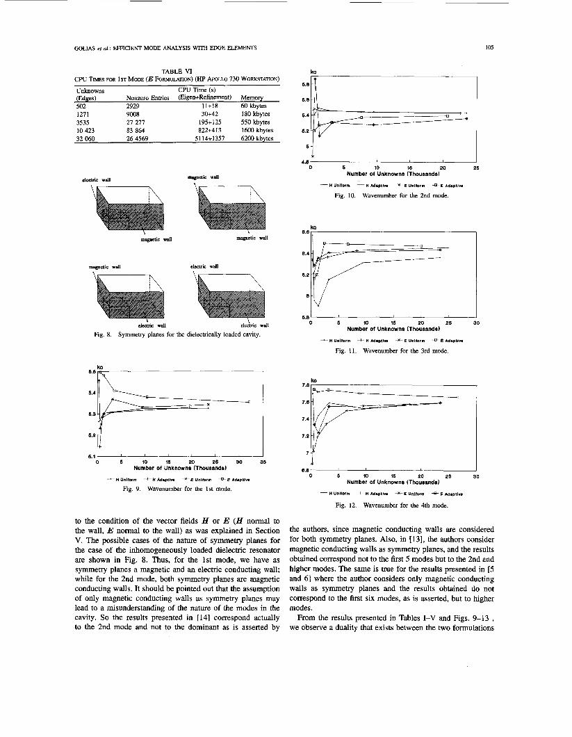
TABLE VI CPU b E S FOR 1ST MODE (E FORMULATION) (HP h L L 0 730 WORKSTATION)

Unknowns CPU Time (s) (Edges) Nonzero Entries (Eigen+Refinement) Memory 502 2929 11+18 60 kbytes 1271 9008 30+42 180 kbytes 3535 27 277 195+125 550 kbytes 10 423 83 864 822+413 1600 kbytes 32 060 26 4569 5114+1357 6200 kbytes

electric wall

magnetic wall magnetic wall

msgnetic wall electric wall

b electric wall

Fig. 8. Symmetry planes for the dielectrically loaded cavity.

ko

ti c

6.1 0 5 10 16 20 26 30 35

Number of Unknowns (Thouranda)

- H Unlform + H Adaptlw + E Unlbrm * E Adaptlw

Fig. 9. Wavenumber for the 1st mode.

to the condition of the vector fields H or E (H normal to the wall, E normal to the wall) as was explained in Section V. The possible cases of the nature of symmetry planes for the case of the inhomogeneously loaded dielectric resonator are shown in Fig. 8. Thus, for the 1st mode, we have as symmetry planes a magnetic and an electric conducting wall; while for the 2nd mode, both symmetry planes are magnetic conducting walls. It should be pointed out that the assumption of only magnetic conducting walls as symmetry planes may lead to a misunderstanding of the nature of the modes in the cavity. So the results presented in [14] correspond actually to the 2nd mode and not to the dominant as is asserted by

ko I +

5.6 6.81i

Y."

0 5 10 15 20 25 30 Number of Unknowns (Thousands)

- n Uniform + n Addlptlw + E Unlform - E Adnptlw

Fig. 11 . Wavenumber for the 3rd mode.

0 5 10 15 20 25 30 Number of Unknowns (Thousands)

- n Unlform + n Adaptlw +E Uniform 4 E Adnptlw

Fig. 12. Wavenumber for the 4th mode.

the authors, since magnetic conducting walls are considered for both symmetry planes. Also, in [13], the authors consider magnetic conducting walls as symmetry planes, and the results obtained correspond not to the first 5 modes but to the 2nd and higher modes. The same is true for the results presented in [5 and 61 where the author considers only magnetic conducting walls as symmetry planes and the results obtained do not correspond to the first six modes, as is asserted, but to higher modes.

From the results presented in Tables I-V and Figs. 9-13 , we observe a duality that exists between the two formulations

106 IEEE TRANSACTIONS

0 5 10 15 20 25 30 6.9

Number of Unknowns (Thoueands)

H Unltorm + n AdapIIva + E Unltorm -+ E Adapllw - Fig. 13. Wavenumber for the 5th mode.

involving the field vectors H and E. It is not clear from the results that the H formulation or the E formulation provide upper or lower bounds of the wavenumber ko. But both formulations converge toward the same value of the wavenum- ber, and this indicates a complementarity that exists between the two formulations [21]. Further, this complementarity and convergence toward the exact value is an indication that the formulations are correct.

IX. CONCLUSION Efficient analysis of 3-D electromagnetic modes in inhomo-

geneously loaded dielectric cavities with edge elements was presented. A self-adaptive refinement algorithm was employed so that an optimum solution is obtained. An error estimator based on the discontinuity of the normal components of the constitutive fields D and B, and allowing the recognition of high enor regions, was proposed for edge elements. Then, with the application of a self-adaptive mesh refinement algorithm, very accurate results were obtained with reduced computa- tional cost. Furthermore, the process of mesh generation is completely automatic, thus freeing the analyst from the heavy work this procedure requires, and thus minimizing man and computer hours.

REFERENCES

[ l ] A. Konrad, “Vectorial variational formulation of electromagnetic fields in anisotropic media,” IEEE Trans. Microwave Theory Tech., vol. M’IT- 24, pp. 553-559, Sept. 1976.

[2] -, “A direct three-dimensional finite element method for the solution of electromagnetic fields in cavities,” IEEE Trans. Mag., vol. 21, pp. 2276-2279, 1985.

[3] -, “On the reduction of the number of spurious modes in the vectorial finite-element solution of three-dimensional cavities and waveguides,” IEEE Trans. Microwave Theory Tech., vol. MTT-34. pp. 54-227, 1986.

141 M. Hara, T. Wada, T. Fukasara, and F. Kikuchi. “Three dimensional .~

analysis of RF electromagnetic fields by finite element method,” IEEE Trans. Mag., vol. MAG-19, pp. 2417-2420, 1983.

[SI J. P. Webb, “Efficient generation of divergence-free field for the finite element analysis of 3D cavity resonances,” IEEE Trans. Mag., vol.

[6] “The finite-element method for finding modes of dielectric loaded cavities,” IEEE Trans. Micmwave Theory Tech., vol. MTT-33, pp. 635-639, July 1985.

[7] A. J. Kobelansky and J. P. Webb, “Eliminating spurious modes in finite element waveguide problems by using divergence free fields,” Elecrron. Lett., vol. 22, no. 11, pp. 569-570, 1986.

MAG-23, pp. 162-165, 1988.

ON MICROWAVE THEORY AND ’ECHNIQUES, VOL. 42, NO. 1, JANUARY 1994

[8] J. P. Webb, G. L. Maile, and R. L. Ferrari, “Finite element solution of three-dimensional electromagnetic problems,” IEE Pmc. vol. 130, pp. - - _. 153-159, Mar. 1983.

[91 J. B. Davies, A. Femandez, and G. Y. Philippou, “Finite element . . analysis of all modes in cavities with circular symmetry,” IEEE Trans. Microwave Theory Tech., vol. MTT-30, pp. 1975-1979, Nov. 1982.

[lo] B. M. A. Rahman and J. B. Davies, “Penalty function improvement of waveguide solution by finite elements,’’ IEEE Trans. Microwave Theory Tech., vol. MTT-32, pp. 922-928, 1984.

[ 111 M. Koshiba, K. Hayata, and M. Suzuki, “Improved finite element formu- lation in terms of the magnetic field vector for dielectric waveguides,” IEEE Trans. Micmwave Theory Tech., vol. MlT-33, pp. 227-233, Mar. 1985.

[12] K. Hayata, M. Koshiba, M. Eguchi, and M. Suzuki, “Vectorial finite element method without any spurious solutions for dielectric waveguid- ing problems using transverse magnetic-field component,” IEEE Trans. Microwave Theory Tech., vol. MlT-34, pp. 1120, 1986.

[13] I. Bardi, 0. Biro, and K. Preis, “Finite element scheme for 3D cavities without spurious modes,” IEEE Trans. Mag., vol. 27, pp. 40364039, Sept. 1991.

[14] L. Pichon and A. Razek, ‘‘Three dimensional mode analysis using edge elements,” IEEE Trans. Mag., vol. 28, pp. 1493-1496, 1992.

1151 A. Bossavit, “A rationale for edge elements in 3D fields computations,” IEEE Trans. Mag., vol. MAG-24, pp. 70-79, 1988.

[ 161 __, “Solving Maxwell equations in a closed cavity and the question of spurious modes,” IEEE Trans. Mug., vol. 26, pp. 702-705, Mar. 1990.

[17] -, “The exploitation of geometrical symmetry in 3-D eddy currents computation,” IEEE Trans. Mag., vol. MAG-21, pp. 2307-2309, Nov. 1985.

(181 J. C. Nedelec, “Mixed finite elements in R3,” Numer. Math., vol. 35,

[ 191 J. F. Lee, D. K. Sun, and 2. J. Cendes, “Tangential vector finite elements for electromagnetic field computation,” IEEE Trans. Mag., vol. 27, pp, 4032-4035, 1991.

[201 N. A. Golias and T. D. Tsiboukis, “Three-dimensional automatic adap- tive mesh generation,” IEEE Trans. Mag., vol. 28, pp. 17W1703, 1992.

1211 P. P. Silvester and R. L. Ferrari, Finite Elements for Electrical Engineers, 2nd ed. Cambridge, U.K.: Cambridge University Press, 1990.

pp. 315-341, 1980.

Nikolaos A. Golias was bom in Vena, Greece, on April 29, 1966. He received the Dipl.Eng. degree from the Department of Electrical Engineering at the Aristotle University of Thessaloniki, Thessaloniki, Greece. in 1989.

Since 1989 he has been a Research Assistant at the Department of Electrical Engineering of the Uni- versity of Thessaloniki, and he is working toward the Ph.D. degree. His current interests are focused on the application of the finite element method to field solution of various engineering problems, and

the development of adaptive techniques in 2 and 3 dimensions. Mr. Golias is a member of the Technical Chamber of Greece

AntonL G. h p g h ~ k i r was bom in ThessaloniLi , Gm=. on January 14,1954. He received the DpL Eng. degree fbm the ELeCeical Engkehg Deparhnent at the Aristotle University of ‘zhessaloniL, Greece, in 1977, and the PhD. degree f” the same institution in 1986. S i 1980 he has been working at the Electrical Engineering Department

of the Aristotle University of TheasaloniLi, w b he is now an W i t Rofhor. His research interests am in the mas of elemomapetic field pmpagation and scatterin& optics, method of moments, and h n ’ e functions methods.

GOLIAS el d.: EFFICIENT MODE ANALYSIS WITH EDGE ELEMENTS

Tbeodoros D. 'kiboukis was born in Larissa, Greece, on February 25. 1948. He received the Dipl. Eng. degree from the National Technical University of Athens, Athens, Greece, in 1971, and the Ph.D. degree from the Aristotle University of Thessaloniki, Thessaloniki, Greece, in 1981.

Since 1981 he has been working in the Department of Electrical Engineering of the Aristotle University of Thessaloniki, where he is now an Associate Professor. He is the author of several books and papers. His research activities

include electromagnetic field analysis by energy methods, with emphasis on the development of special finite element techniques to field solution of various engineering applications. Dr. Tsiboukis is a member of the Technical Chamber of Greece.