adaptive mesh and algorithm refinement using direct … · adaptive mesh and algorithm refinement...

Journal of Computational Physics154,134–155 (1999)

Article ID jcph.1999.6305, available online at http://www.idealibrary.com on

Adaptive Mesh and Algorithm RefinementUsing Direct Simulation Monte Carlo

Alejandro L. Garcia,∗,1 John B. Bell,∗ William Y. Crutchfield,∗ and Berni J. Alder†∗Center for Computational Sciences and Engineering, Lawrence Berkeley National Laboratory, Berkeley,

California 94720;†Lawrence Livermore National Laboratory, Livermore, California 94550E-mail: [email protected], [email protected], [email protected], [email protected]

Received February 15, 1999; revised May 10, 1999

Adaptive mesh and algorithm refinement (AMAR) embeds a particle methodwithin a continuum method at the finest level of an adaptive mesh refinement (AMR)hierarchy. The coupling between the particle region and the overlaying continuumgrid is algorithmically equivalent to that between the fine and coarse levels of AMR.Direct simulation Monte Carlo (DSMC) is used as the particle algorithm embeddedwithin a Godunov-type compressible Navier–Stokes solver. Several examples arepresented and compared with purely continuum calculations.c© 1999 Academic Press

1. INTRODUCTION

When a large range of scales must be spanned, computational fluid dynamics (CFD)calculations often employ local mesh refinement so that a fine grid is used only in thoseregions that require high resolution. However, hydrodynamic formulations break down asthe grid spacing approaches the molecular scale, for example, the mean free path in agas. This paper describes adaptive mesh and algorithm refinement (AMAR), in which acontinuum algorithm, such as a Navier–Stokes solver, is replaced by a particle algorithm,such as direct simulation Monte Carlo (DSMC), at the finest grid scale.

As an illustration, consider the flow of a gas through a microscopic channel, such asbetween the head and platter in a disk drive [1]. The continuum description of the flow andthe quantities derived from it, such as wall drag, are not accurate whenever the Knudsennumber Kn> 10−2, where Kn≡ λ/L, λ is the mean free path andL is the channel width [2]Kinetic theory extensions to the continuum equations (e.g., Burnett expansion) have hadlimited success [3]. Another approach is to introduce kinetic corrections to the boundaryconditions but these are often not accurate [1, 4, 5] and can even give wrongqualitativefeatures of the flow [6].

1 Permanent address: Physics Department, San Jose State University, San Jose, CA 95192.

134

0021-9991/99 $30.00Copyright c© 1999 by Academic PressAll rights of reproduction in any form reserved.

ADAPTIVE MESH AND ALGORITHM REFINEMENT 135

Rigorously, a kinetic formulation is required at microscopic scales, however, at hydro-dynamic scales the continuum approximation is valid. AMAR uses a particle method inregions of a flow requiring microscopic resolution and a continuum method, with varyinglevels of refinement, to evaluate the flow at larger scales. Thus, AMAR provides an effec-tive methodology to span a broad range of length scales while retaining the advantages ofa kinetic formulation where required.

At both rarefied and atmospheric densities the best particle method to use is direct sim-ulation Monte Carlo. DSMC is several orders of magnitude more efficient than moleculardynamics for the simulation of gases; however, it remains several orders of magnitude lessefficient than continuum CFD methods. For these reasons several researchers have investi-gated coupling the DSMC algorithm to a hydrodynamic solver. There exist loosely coupledschemes for which a continuum method provides a boundary condition for a DSMC code [7]or in which the two methods calculate different quantities in the problem (e.g., continuummethod for the flow field and a particle method for the chemistry [8]). However, the focushere is on strongly coupled schemes where the DSMC and continuum methods simultane-ously evaluate different regions of the flow and continuously exchange information acrossan interface.

Wadsworth and Erwin first demonstrated such a scheme in calculating a one-dimensionalshock wave profile [9] and a two-dimensional slit flow [10]. Related hybrid schemes weredeveloped by Eggers and Beylich [11], Bourgatet al.[12], Le Tallec and Mallinger [13], andthe author [14, 15]. Hash and Hassan performed detailed studies of a DSMC/Navier–Stokeshybrid using the Marshak condition for resolving fluxes [16]. They also demonstrated thata Chapman–Enskog distribution was required when the viscous fluxes were significant butthat a simple Maxwellian distribution was adequate when the continuum region was wellapproximated by the Euler equations [7]. Special purpose continuum solvers, which areclosely tied to kinetic theory, have been proposed for use in hybrid schemes. Specifically,the kinetic flux-vector splitting (KFVS) [17] and adaptive discrete velocity (ADV) Eulersolver [18] have been tested.

While adaptive mesh and algorithm refinement may superficially resemble other hybridschemes, it differs fundamentally from all of them. First, AMAR is specifically designed towork as a multi-level method for simulating systems whose length scales span several ordersof magnitude. AMAR is a natural extension of adaptive mesh refinement (AMR) and caneasily be implemented within an existing AMR code. Second, the AMAR coupling betweenthe particle and continuum regions conserves mass, momentum, and energy to within round-off error. Not only does this eliminate any systematic drift in the solution (e.g., mass loss in aclosed system), it also improves the numerical stability of the method. Third, the continuumsolver can easily be changed to any conservative (i.e., flux-based) scheme, either implicit orexplicit. Only four basic subroutines, outlined at the end of Section 4, couple the continuumsolver to the particle algorithm. Finally, some hybrids schemes are limited, in theory orin practice, to the simulation of one- or two-dimensional problems; AMAR is fully threedimensional.

This paper presents the framework for adaptive mesh and algorithm refinement andillustrates its use by incorporating a DSMC simulation at the finest level of an adaptivemesh refinement hierarchy. The DSMC algorithm and AMR scheme are briefly describedin Sections 2 and 3. The AMAR technique for coupling these methods is presented inSection 4 and results from AMAR calculations in Section 5. Finally, Section 6 describesfuture work.

136 GARCIA ET AL.

2. DIRECT SIMULATION MONTE CARLO

Direct simulation Monte Carlo (DSMC) is a well-established algorithm for computing gasdynamics at the level of the Boltzmann equation. For completeness, this section presentsa summary of the method, emphasizing those elements that are relevant to formulatingAMAR. The DSMC algorithm is described in detail in [19]; see [20] for a tutorial and[21, 22] for reviews.

In DSMC, the state of the system is given by the positions and velocities of particles,{r i , vi }. First, the particles are moved as if they did not interact, that is, their positions areupdated tor i + vi1t . Any particles that reach a boundary are processed according to theappropriate boundary condition. Second, after all particles have moved, a given numberare randomly selected for collisions. This splitting of the evolution between streaming andcollisions is only accurate when the time step,1t , is a fraction of the mean collision timefor a particle.

The concept of “collision” implies that the interaction potential between particles isshort-ranged. In the simulations presented here the particles are taken to be rigid spheres ofdiameterσ . Extensions to other representations of the molecular interaction may be used togive more realistic transport properties [19] and equations of state [23, 24]. For hard sphereparticles, the number of collisions amongN particles in a cell volumeV during a time step is

M = N2πσ 2〈vr〉1t

2V, (1)

where〈vr〉 is the average relative speed among the particles. Bird’s “no time counter” method[19] for computing collision frequency is used since it avoids the explicit evaluation of〈vr〉.

Particles are randomly selected as collision partners with the restriction that their meanseparation be a fraction of a mean free path [25]. This restriction is enforced by ensuring thatcell dimensions are less than a mean free path. For hard spheres, the probability of selectinga given pair is proportional to the relative speed between the particles. DSMC evaluatesindividual collisions stochastically, conserving momentum and energy and selecting thepost-collision angles from their kinetic theory distributions. For hard spheres, the centerof mass velocity and relative speed are conserved in the collision with the direction of therelative velocity uniformly distributed in the unit sphere. This Markov approximation ofthe collision process is statistically accurate so long as the number of particles in a collisioncell is sufficiently large, typically over twenty [26, 27].

These constraints on time step, cell size, and number of particles make DSMC compu-tationally expensive unless the physical domain is small or the gas is highly rarefied. Forexample, the efficiency of the method can be judged by the observation that a simulation ofair at standard temperature and pressure requires about 106 particles per cubic micron and104 time steps per microsecond.

3. ADAPTIVE MESH REFINEMENT

In a computational fluid dynamics calculation, the standard hydrodynamic variables aredensityρ, fluid velocity u= [ux uy uz], and pressureP. From these one may obtain theconserved densities of massρ, momentump, and energy,e. The compressible Navier–Stokes equations may be written in the conservative form [28],

∂U∂t+∇ · F = ∇ · D, (2)


whereU is a vector composed of the conserved densities,F= (Fx,Fy,Fz) represent thehyperbolic flux terms, andD= (Dx,Dy,Dz) the parabolic flux terms. More precisely,

U =

ρ

px

py

pz

e

; Fx =

ρux

ρu2x + Pρuxuy

ρuxuz

(e+ P)ux

; Dx =

0τxx

τxy

τxz

ui τxi − qx

, (3)

whereτ andq are the stress tensor and heat flux, respectively, with similar expressions forthe other flux terms.

In the AMAR methodology presented here, the compressible Navier–Stokes equationsare integrated using a second-order unsplit Godunov method to evaluate the hyperbolicfluxes [29] and a standard finite difference approximation using Crank–Nicolson temporaldifferencing to treat the parabolic terms. Thus, the discretization has the form

Un+1i jk − Un

i jk

1t+

Fx,n+ 1

2

i+ 12 , j,k− F

x,n+ 12

i− 12 , j,k

1x+

Fy,n+ 1

2

i, j+ 12 ,k− F

y,n+ 12

i, j− 12 ,k

1y+

Fz,n+ 1

2

i, j,k+ 12− F

z,n+ 12

i, j,k− 12

1z

= 1

2

(Dx,n+1

i+ 12 , j,k+ Dx,n

i+ 12 , j,k− Dx,n+1

i− 12 , j,k− Dx,n

i− 12 , j,k

1x

+Dy,n+1

i, j+ 12 ,k+ Dy,n

i, j+ 12 ,k− Dy,n+1

i, j− 12 ,k− Dy,n

i, j− 12 ,k

1y

+Dz,n+1

i, j,k+ 12− Dz,n

i, j,k+ 12− Dz,n+1

i, j,k− 12− Dz,n

i, j,k− 12

1z

). (4)

The implicit discretization of the parabolic terms requires the solution of a nonlinear sys-tem of equations which is easily treated using standard nonlinear multigrid ideas. Thecomputation of the hyperbolic flux terms using the second-order Godunov procedure is anexplicit procedure so that the integration algorithm has a time step restriction based on CFLconsiderations for the Euler equations(D= 0).

For problems in fluid dynamics where there are a large range of scales that must bespanned, some form of adaptive mesh refinement is used to localize high resolution tothe areas where it is required. In the AMR methodology, a block-structured hierarchicalform of refinement, first developed by Berger and Oliger [30] for hyperbolic partial dif-ferential equations, is used. A conservative version of this methodology for gas dynamicswas developed by Berger and Colella [31] and extended to three dimensions by Bellet al.[32].

AMR is based on a sequence of nested levels of refinement with successively finer spacingin both time and space. In this approach, fine grids are formed by dividing coarse cells bya refinement ratio,r , in each direction. Increasingly finer grids are recursively embeddedin coarse grids until the solution is adequately resolved with each level contained in thenext coarser level. An error estimation procedure based on user-specified criteria evaluateswhere additional refinement is needed and grid generation procedures dynamically createor remove rectangular fine grid patches as resolution requirements change.

The adaptive time-step algorithm advances grids at different levels using time stepsappropriate to that level based on CFL considerations. The time-step procedure can most

138 GARCIA ET AL.

easily be thought of as a recursive algorithm, in which to advance levell (level l = 0 beingthe coarsest andl = lmax the finest), the following steps are taken:

• Advance levell in time as if it is the only level. Supply boundary conditions forUfrom levell − 1 if level l > 0, and from the physical boundary conditions.• If l < lmax

—Advance level (l + 1) r times with time step1t l+1= 1r 1t l using boundary con-

ditions forU from levell , and from the physical domain boundaries.—Synchronize the data between levelsl and l + 1, and interpolate corrections to

higher levels ifl + 1< lmax.

The adaptive algorithm, as outlined above, performs operations to advance each levelindependent of other levels in the hierarchy (except for boundary conditions) and thencomputes a correction to synchronize the levels. Loosely speaking, the objective in thissynchronization step is to compute the modifications to the coarse grid that reflect thechange in the coarse grid solution from the presence of the fine grid. There are two steps inthe synchronization. First, the fine grid is averaged onto the coarse grid; i.e., the conservedquantities on coarse grid cells covered by fine grid are replaced by the average of the finegrid.

The second step of the synchronization, called “refluxing,” corrects for the difference incoarse and fine grid fluxes at the boundary of the fine grid. The basic approach used hereis an analog of the procedure used by Almgrenet al. [33] extended to the case of nonlinearparabolic terms. During the course of the integration step, flux information is saved at thefaces on the boundary of the coarse and fine grid to obtain the difference between the fluxescalculated at levell and the corresponding levell + 1 average. The latter are the fluxes atlevel l + 1 time averaged over the levell time step and spatially averaged over the area ofthe levell face. This time step- and area-weighted flux difference is

δF l = 1t l

(−Al

(Fn+ 1

2 ,l − 1

2(Dn,l + Dn+1,l )

)

+ 1

r

r−1∑k=0

∑faces

Al+1

(Frn+k+ 1

2 ,l+1− 1

2(Drn+k,l+1+ Drn+k+1,l+1)

)), (5)

whereF andD are the components of the convective and diffusive fluxes corresponding tothe faces in Eq. (4) andA is the signed area of the face of a grid cell where the sign dependson the direction normal to the face, facing away from the fine grid. The sum over faces inEq. (5) is a sum over all fine grid faces that cover the coarse face.

The flux correction,δF ln, represents the difference between the flux used to update the

coarse cells adjacent to the fine grid and the fluxes that are computed on the fine grid.To ensure stability for low Reynolds numbers and to match the implicit, Crank–Nicolsoncharacter of the diffusive step an implicit solve is performed

δU− 1t

2∇ · D(Un+1+ δU) = 1tδF

1x1y1z, (6)

whereUn+1 is the coarse grid solution after averaging the fine grid solution but beforecomputing the correction. The coarse grid,Un+1, is updated by

Un+1 = Un+1+ δU. (7)


The fine grid is updated by using a conservative scheme that interpolates the correction tothe fine grid and to other finer grids contained within the fine grid. Finally, to capture theeffect of the synchronization of levell and higher on levell − 1 the flux correctionsF l−1

are not updated until after the synchronization of levelsl andl + 1.

4. ADAPTIVE MESH AND ALGORITHM REFINEMENT

Adaptive mesh and algorithm refinement (AMAR) uses the same basic algorithmic outlineas AMR, as presented in the previous section, except that the finest grid level is evaluatedby a DSMC calculation. For the purposes of exposition, a DSMC region is consideredembedded within a single-level continuum grid.

At the start of a continuum time step, fluxes are computed at each cell face and used toadvance the conserved densities (mass, momentum, and energy) on the grid. All continuumcells are advanced by1tcont, including those that overlay the DSMC region. For numericalstability,1tcont=C1x/|c+ v| wherec is the sound speed,v is the maximum fluid speed,andC< 1 is the Courant number. Next, the particle calculation advances to the same time bytaking several, smaller time steps,1tpart. Though1tpart is a fraction of the mean collisiontime, for the finest continuum grid1x≈ λ so1tc≈1tpart. For the AMAR calculationspresented in this paper, the width of the smallest continuum cells is two mean free pathsand1tcont< 41tpart.

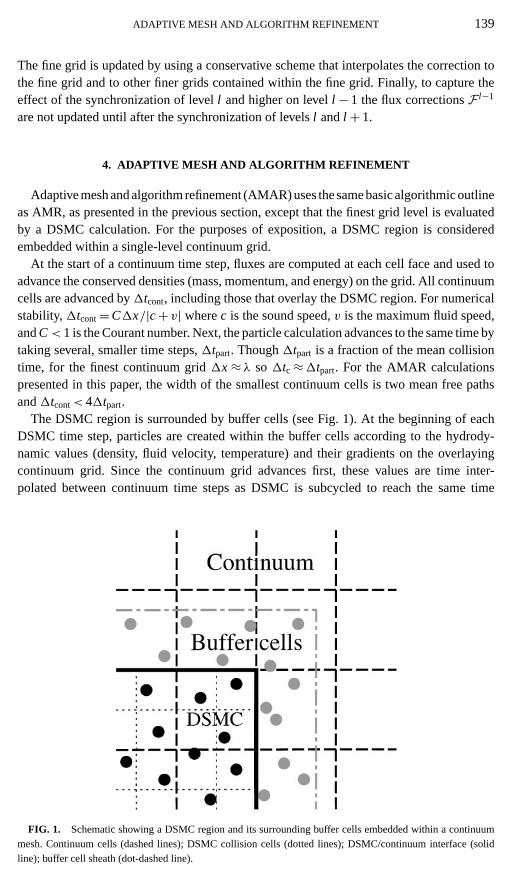
The DSMC region is surrounded by buffer cells (see Fig. 1). At the beginning of eachDSMC time step, particles are created within the buffer cells according to the hydrody-namic values (density, fluid velocity, temperature) and their gradients on the overlayingcontinuum grid. Since the continuum grid advances first, these values are time inter-polated between continuum time steps as DSMC is subcycled to reach the same time

FIG. 1. Schematic showing a DSMC region and its surrounding buffer cells embedded within a continuummesh. Continuum cells (dashed lines); DSMC collision cells (dotted lines); DSMC/continuum interface (solidline); buffer cell sheath (dot-dashed line).

140 GARCIA ET AL.

as the continuum solver. Buffer cells do not need to be entirely filled with particles.Only particles within a sheath near the DSMC region are generated with the thicknessof this sheath determined adaptively. The particle velocities are drawn from the appro-priate distribution for the continuum solver: the Maxwell–Boltzmann distribution for theEuler equations and the Chapman–Enskog distribution [34] for the Navier–Stokes equa-tions.

Next, particles in both the main and buffer regions move a single DSMC time step. Ifa particle crosses the interface between these regions, that particle contributes to the fluxfor the coarse grid face through which it passes. The contribution of all particles crossinga coarse grid face during the DSMC steps plays the same role as the sum over fine-gridcontinuum grid faces in Eq. (5). After moving the particles, those remaining in or those thatmoved into the buffer region are discarded and collisions among the remaining particlesare evaluated. The cell structure used in evaluating DSMC collisions is separate from andindependent of the continuum grid.

A technical but important issue that any particle/continuum hybrid must confront is the“corner problem.” Specifically, when a particle passes into the continuum region, it changesthe mass, momentum, and energy density in a continuum cell. In AMAR, this particle’scontribution is formulated as a flux on the cell side that lies on the interface between thecontinuum and particle regions. A similar flux contribution arises when a particle createdwithin the buffer region crosses this interface. For example, in Fig. 2, when particle 1 passesfrom cell A to D (or vice versa), it contributes to the flux on the side between these cells.A more complicated case occurs when particle 2 passes from cell B to D. AMAR updatesthe flux on the side between cells B and E since that is where the particle crosses theinterface. Finally, consider particle 3, which passes near the corner traveling from cell Bto F. This particle contributes to the flux between cells B and C. There cannot be a fluxcontribution for cell F since it has no side bordering the particle/continuum interface. Thislast example illustrates that fluxes must be evaluated where a particle crosses the interfaceand not from the cell that the particle moves into. If a simulation does not handle the cornerscorrectly, steady state flows can exhibit a spurious drift, such as loss of mass in a closedsystem.

FIG. 2. Particles and continuum cells near a corner of the DSMC/continuum interface.


When the DSMC region has advanced for an entire continuum grid time step, two synchro-nizations are performed, analogous to the AMR case described above. First, the continuumcells that overlay the central DSMC region are reset according to the conserved densitiescomputed from the set of particles within each continuum grid cell. Second, Eq. (6) is solvedto obtain a correction to the fluxes for the continuum grid using as right hand side

δF l = 1t l

(−Al

(Fn+ 1

2 ,l − 1

2(Dn,l − Dn+1,l )

))+∑

p

Fp, (8)

where the sum represents the flux of the conserved quantities through carried by particlesppassing through the coarse face during the DSMC updates. Equation (7) is used to updatethe conserved quantities on the coarse grid.

From the implicit solve in Eq. (6), the values ofδU on coarse cells covered by the DSMCregion generate a correctionδp andδe in the momenta and energy for DSMC cells; thereis no mass correction because mass does not diffuse. The velocity of each particle within agiven continuum cell is corrected as

v′ = 〈v′〉 + α(v− 〈v〉), (9)

where〈v′〉 = 〈v〉 + δp/ρ,

α=(

1+ δe+ ek − e′ke− ek

)1/2

, (10)

with ek= 12ρ|〈v〉|2, e′k= 1

2ρ|〈v′〉|2, ande= 12ρ〈|v|2〉; the angle brackets indicate averages

over particles within a continuum cell. These synchronization steps guarantee that, in theabsence of external sources, total mass, momentum, and energy are conserved to withinround-off error in the computational domain. Note that when an explicit solver is used,as with the Euler equations, the correction is localized to the coarse cells adjacent to theDSMC region so no correction to the particles is required.

In summary, the interaction between the continuum solver and the DSMC region isencapsulated into four routines: (1) Passing the time-interpolated state to the particle buffercells; (2) Passing the momentum and energy corrections, as computed in the implicit linearsolve, to the DSMC region; (3) Receiving the fluxes recorded when particles cross theDSMC interface; (4) Receiving conserved densities for continuum cells overlaying theDSMC region. This coupling of the continuum grid with DSMC makes the latter appearjust like any level of refinement in the purely continuum case.

5. NUMERICAL EXAMPLES

This section describes a series of numerical experiments that were performed to test anddemonstrate the adaptive mesh and algorithm refinement framework. In each case a singleDSMC region is embedded within a continuum grid on which either the Euler or Navier–Stokes equations are computed. In general, the particles in the buffer regions are generatedusing the Chapman–Enskog distribution [34]. However, for the purpose of comparison,when the Euler equations are used, both the Maxwell–Boltzmann and Chapman–Enskogdistributions are considered. In the last example (flow past a sphere) the continuum solver

142 GARCIA ET AL.

uses two grid levels so the DSMC region is embedded within a fine grid which is itselfembedded in a coarse grid. For all other examples, a single continuum grid is used.

The particles are treated as hard spheres of diameterσ = 0.366 nm and massm= 6.63×10−23 g (argon parameters). The reference density isρ0= 1.78× 10−3 g/cm3; the meanfree path at this density isλ0= 62.5 nm. The reference temperature isT0= 273 K and thereference sound speed isc0= 3.08× 104 cm/s. The equation of state is the ideal gas law,P= ρkT/m, wherek= 1.3806× 10−23 J/K is Boltzmann’s constant. The viscosity andthermal conductivity are

µ = 5

16d2

√mkT

π; κ = 15k

4mµ, (11)

as given by the Chapman–Enskog theory.All the simulations are fully three dimensional with at least 16 continuum grid cells in

each direction. When a single grid is used, these cells are cubes of length1x= 2λ0; whenthere are two continuum levels, the cells are cubes of length1x and 21x. The referenceCFL time step is1t0=1x/c0= 4.06× 10−10 s and the Courant number is 0.25 for all ofthe runs. With this Courant number the DSMC region typically performs from one to fourtime steps for each continuum time step.

At the reference density, the DSMC region contains 100 particles perλ30. The collision

frequency is computed using cubic cells of length 1.0λ0, collision partners are selectedwithin cubic subcells of length 0.5λ0, and statistical samples are measured in cubes oflength 0.8λ0. The total number of particles in the various cases ranges from 5× 104 to6× 106.

5.1. Thermodynamic Equilibrium

The simplest test case is thermodynamic equilibrium: the system is initially at rest withconstant density and temperature. The continuum grid is 32× 32× 32 with periodic bound-ary conditions on all sides. The DSMC region is a cube embedded in the continuum solverwithin the 4× 4× 4 cells at the center of the system. Although the system is initially uni-form, DSMC produces spontaneous fluctuations with the correct equilibrium spectrum [35].After 2000 continuum time steps, the total mass in the simulation is conserved to betterthan one part in 106 and the total energy to better than one part in 105.

When the continuum solver employs the Navier–Stokes equations, the system remains inthermodynamic equilibrium. However, when the Euler equations are used in the continuumregion, the number of particles in the DSMC region slowly increases and the energy densitydecreases so that thermodynamic equilibrium is not maintained. Since total mass, momen-tum, and energy are strictly conserved (to within round-off error), the mass in the continuumregion decreases and the energy density increases. This rise in the number of DSMC par-ticles as a function of time is shown in Fig. 3. While the Navier–Stokes/AMAR preservesthe correct average, after 2000 steps the number of DSMC particles in the Euler/AMARincreases by 1.1% when using the Maxwell–Boltzman distribution in the buffer region andby 0.7% when using the Chapman–Enskog distribution. This error is reduced when thesimulation uses more particles per cubic mean free path. For the runs displayed in Fig. 3each continuum cell that overlays the DSMC region contains, on average, 800 particles.

The anomalous drift away from thermodynamic equilibrium that is observed using theEuler equations isnot a flaw in the AMAR methodology. Other DSMC/Euler coupling


FIG. 3. Number of particles in the DSMC region versus time step for thermodynamic equilibrium. EulerAMAR using Maxwell–Boltzmann (×), Chapman–Enskog (+) compared with the Navier–Stokes AMAR (©)which varies about the initial value (dashed line).

schemes also exhibit this drift at equilibrium [36, 37]. The effect is due to the fact thatfluctuations in the DSMC region transmit thermal and mechanical energy to the continuumregion while only mechanical energy is returned since the Euler equations have no heatflux even when a temperature gradient is present. Thus the thermal energy in the continuumregion rises and the density falls so as to maintain mechanical equilibrium (i.e., constantpressure). This spurious effect is masked when there is a net flow across the system. Ifthe simulation is initialized with a uniform fluid speed of 0.05c0, after 2000 time steps thenumber of DSMC particles in the Euler AMAR increases by 0.6% when using the Maxwell–Boltzman distribution in the buffer region and by 0.4% when using the Chapman–Enskogdistribution.

5.2. Impulsive Piston

The first non-equilibrium case considered is a gas initially at the reference density andtemperature and moving at Mach 2 toward a thermal wall held at fixed temperature (Fig. 4a).This is equivalent to an impulsively started piston traveling into a gas initially at rest, in thereference frame of the piston. A normal shock develops in front of the wall and the shockfront moves into the gas. Basic shock relations [38] give a shock speed of Mach 3, a densityratio of 3 across the shock, and a temperature ratio of 11/3. The reference temperature in theundisturbed gas is 273 K so the wall temperature is fixed at 1001 K. The boundary conditionon the opposite side of the system is a plane of reflection symmetry. The flow near thatboundary (a rarefaction fan) does not affect the shock wave within the time of the simulationand thus is not analyzed. Periodic boundary conditions are applied in the other directions.

144 GARCIA ET AL.

FIG. 4. Geometry for (a) impulsively started piston; (b) Rayleigh problem; (c) flow past a sphere.

The continuum grid contains 100× 16× 16 cells leading to a system of length 12500 nm,width and depth of 2000 nm. The DSMC region, located next to the wall where the shockforms, has width and depth of 2000 nm and length of either 625 or 1250 nm, equivalentto 5 or 10 continuum cells. In the larger DSMC simulation the number of particles isinitially 2× 106 and finally 6× 106 when the shock passes into the continuum region. Forcomparison, a calculation with only the Navier–Stokes solver and no DSMC region is alsoconsidered.

Figures 5 and 6 show the temperature and density profiles near the piston wall att = 2× 10−9 s. For the AMAR run with the 5 cell DSMC region, the shock is just passingout of the particle region and it is in the center of the region for the 10 cell DSMC run.The latter run is practically equivalent to a purely DSMC simulation with fixed reservoirssince the values in the Navier–Stokes region are constant. The AMAR runs are in goodagreement with each other; as expected, the temperature profile in the entire continuum run

FIG. 5. Temperature versus position for the impulsively started piston att = 2× 10−9 s. AMAR run with5-cell DSMC region (©); AMAR run with 10-cell DSMC region (3); and purely continuum with no DSMC run(+). Open symbols, DSMC data; filled symbols, AMAR continuum data. Dashed lines indicate the location of theparticle/continuum interface for the AMAR runs.


FIG. 6. Density versus position for the impulsively started piston att = 2× 10−9 s. See Fig. 5 for legend.

lags the DSMC data while the density profile is in better agreement [19]. The temperatureand density profiles near the piston wall att = 4× 10−9 s are shown in Figs. 7 and 8. Thetemperature profiles of the two AMAR runs are again in good agreement while the densityprofiles are in fair agreement.

The impulsive piston is a severe test of the AMAR method since it is well known thatthe Navier–Stokes equations do not accurately predict the profiles of strong shocks. This isbecause the Chapman–Enskog expansion, on which the equations are based, breaks downwhen the characteristic length scale of hydrodynamic gradients is comparable to the meanfree path. A breakdown parameter for the Chapman–Enskog distribution [34] is defined asB= max{|τ ∗i j |, |q∗i |}, where

τ ∗i j =µ

P

(∂ui

∂xj+ ∂u j

∂xi− 2

3

∂uk

∂xkδi j

)(12)

FIG. 7. Temperature versus position for the impulsively started piston att = 4× 10−9 s. See Fig. 5 for legend.

146 GARCIA ET AL.

FIG. 8. Density versus position for the impulsively started piston att = 4× 10−9 s. See Fig. 5 for legend.

and

q∗i = −κ

P

(2m

kT

)1/2∂T

∂xi(13)

are the normalized stress tensor and heat flux, respectively. This parameter is computed whenthe particle velocities are generated in the buffer regions; the validity of the distribution isquestionable whenB> 0.2. In the AMAR simulations of the impulsive piston, the maximumvalue ofB was 1.3–1.4. For comparison, in the simulations of thermodynamic equilibriumB is not zero due to spontaneous fluctuations yet it did not exceed 0.13.

For the impulsive piston, the Euler AMAR program produces results similar to thosepresented above. The Euler equations are adequate for this flow since the advective fluxesare much greater than the dissipative fluxes. The main differences are that the shock thicknessdepends on the solver’s numerical viscosity and that outside the DSMC region the densityand temperature profiles of the shock front overlap. These differences between the Eulerand Navier–Stokes solutions exist independent of whether or not the simulation includes aDSMC region.

5.3. Rayleigh Problem

This problem concerns a gas initially at the reference density and temperature moving atMach 2 parallel to a stationary wall held at the reference temperature (Fig. 4b). This is theRayleigh problem of an impulsively started wall shearing a gas initially at rest, as viewedin the reference frame of the moving wall. In time, the wall drags the gas to match its speedand the resulting velocity gradient produces viscous heating near the wall. The boundarycondition on the opposite side is a plane of reflection symmetry; for short times the gas nearthis boundary remains undisturbed. Periodic boundary conditions are applied in the otherdirections.

The continuum grid contains 100× 16× 16 cells, corresponding to a system of length12,500 nm with width and depth of 2000 nm. The DSMC region, located next to the thermalwall has width and depth of 2000 nm, and length of either 625 or 1250 nm, correspondingto either 5 or 10 continuum cells. In the larger DSMC simulation the number of particles


FIG. 9. Momentum density parallel to the wall versus position for the Rayleigh problem. AMAR run with5-cell DSMC region (©); AMAR run with 10-cell DSMC region (3); and purely continuum with no DSMC run(+). Open symbols DSMC data; filled symbols AMAR continuum data. Dashed lines indicate the location of theparticle/continuum interface for the AMAR runs.

remains steady at about 2× 106. For comparison, a calculation with only the Navier–Stokessolver and no DSMC region is also evaluated. Since the flow is entirely due to viscous drag,an Euler AMAR is not considered.

Figure 9 shows the component of momentum density parallel to the wall att = 7.0×10−9 s. Note that there is good agreement between the two AMAR runs. The continuumsolver uses no-slip boundary conditions at the thermal wall and thus fails to capture theKnudsen velocity slip at the wall. The slip length, that is, the distance within the wall atwhich the velocity extrapolates to zero, is 69 nm, approximately one mean free path asexpected from kinetic theory [2]. The normal component of momentum density is shownin Fig. 10. Because the flow in this direction is relatively weak, fluctuations are noticeablein the data points within the DSMC regions. Again, the two AMAR runs are in agreementand differ significantly from the purely continuum run.

FIG. 10. Normal momentum density versus position for the Rayleigh problem. See Fig. 9 for legend.

148 GARCIA ET AL.

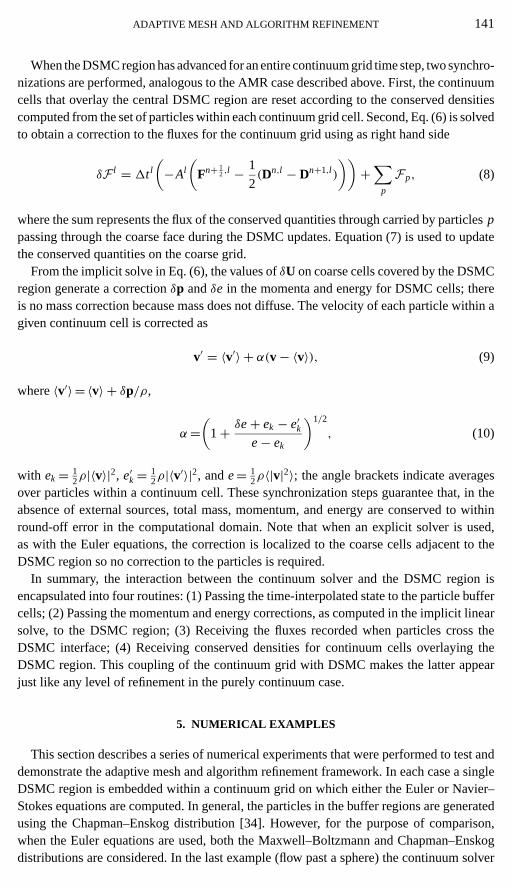
FIG. 11. Temperature versus position for the Rayleigh problem. See Fig. 9 for legend.

The flow away from the wall is due to the pressure gradient that develops when thetemperature rises due to viscous heating (Fig. 11). The AMAR runs reproduce the Knudsentemperature jump at the wall. The distance within the wall at which the temperature profileextrapolates to the temperature of the wall is 120 nm, approximately15

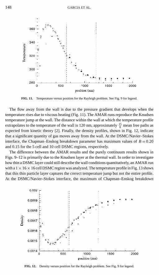
8 mean free paths asexpected from kinetic theory [2]. Finally, the density profiles, shown in Fig. 12, indicatethat a significant quantity of gas moves away from the wall. At the DSMC/Navier–Stokesinterface, the Chapman–Enskog breakdown parameter has maximum values ofB= 0.20and 0.15 for the 5 cell and 10 cell DSMC regions, respectively.

The difference between the AMAR results and the purely continuum results shown inFigs. 9–12 is primarily due to the Knudsen layer at the thermal wall. In order to investigatehow thin a DSMC layer could still describe the wall conditions quantitatively, an AMAR runwith a 1× 16× 16 cell DSMC region was analyzed. The temperature profile in Fig. 13 showsthat this thin particle layer captures the correct temperature jump but not the entire profile.At the DSMC/Navier–Stokes interface, the maximum of Chapman–Enskog breakdown

FIG. 12. Density versus position for the Rayleigh problem. See Fig. 9 for legend.


FIG. 13. Temperature versus position for the Rayleigh problem. AMAR run with 1-cell DSMC region (h);other symbols and lines as in Fig. 9.

parameter isB= 0.50, which further indicates that the DSMC/continuum interface is tooclose to the wall.

5.4. Flow Past a Sphere

As a final example, flow past a microscopic object was considered. The body is a sphereheld at the reference temperature and fixed at the center of the system (Fig. 4c). Inflowconditions are Mach 1 flow at the reference density and temperature. The continuum solveruses characteristic outflow boundary conditions with no diffusive fluxes. Periodic boundaryconditions are applied in the other directions. While the flow is axially symmetric for thissimple body, the calculation is fully three dimensional to demonstrate AMAR’s capacity tosimulate large scale flows.

The continuum solver uses two grids: a fine mesh embedded within a coarse mesh. Thelatter spans the entire system and contains 32× 32× 32 coarse cells covering the systemsize of 8000 nm in each direction. The fine mesh covers a cube of length 4000 nm locatedat the center of the system. The DSMC region is a cube of length 1000 nm embedded in thecenter of the fine mesh. The DSMC region contains some 4× 105 particles and occupiesless than 0.2% of the total volume; see Fig. 14.

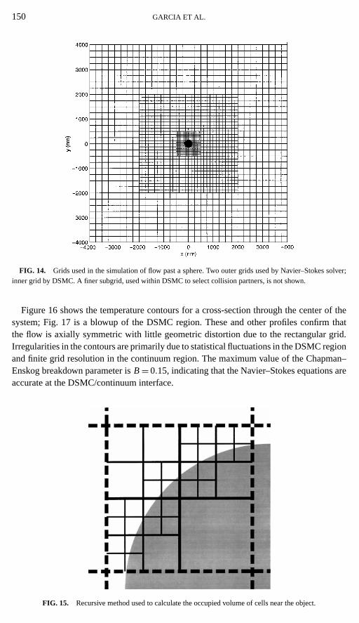
For both the continuum grid cells and the DSMC cells, the fractional volume occupied bythe sphere is computed by a recursive method (Fig. 15). A cell is bisected in each direction;each corner of these subcells lies either inside or outside the body. If all corners are occupied(or empty), the fractional occupied volume for that subcell is one (or zero). Subcells whichare partially occupied are further subdivided and this recursion continues until the desiredaccuracy is obtained. When the deepest level of recursion is reached, a subcell’s occupiedvolume is estimated from the number of occupied corners.

The diameter of the sphere is 5λ0 (312 nm) thus Kn= 0.2. For Mach number Ma= 1 theReynolds number is Re= 8.24. For these Knudsen and Reynolds numbers solutions of theBoltzmann equation predict a drag coefficient ofCD = 1.95 when Ma¿ 1 [39]. A standingring-eddy forms behind the sphere at Re> 24 [40] but since this numerical experiment iswell below the critical Reynolds number vortices are not expected to form.

150 GARCIA ET AL.

FIG. 14. Grids used in the simulation of flow past a sphere. Two outer grids used by Navier–Stokes solver;inner grid by DSMC. A finer subgrid, used within DSMC to select collision partners, is not shown.

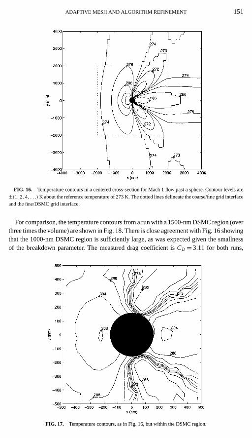
Figure 16 shows the temperature contours for a cross-section through the center of thesystem; Fig. 17 is a blowup of the DSMC region. These and other profiles confirm thatthe flow is axially symmetric with little geometric distortion due to the rectangular grid.Irregularities in the contours are primarily due to statistical fluctuations in the DSMC regionand finite grid resolution in the continuum region. The maximum value of the Chapman–Enskog breakdown parameter isB= 0.15, indicating that the Navier–Stokes equations areaccurate at the DSMC/continuum interface.

FIG. 15. Recursive method used to calculate the occupied volume of cells near the object.


FIG. 16. Temperature contours in a centered cross-section for Mach 1 flow past a sphere. Contour levels are±(1, 2, 4, . . .)K about the reference temperature of 273 K. The dotted lines delineate the coarse/fine grid interfaceand the fine/DSMC grid interface.

For comparison, the temperature contours from a run with a 1500-nm DSMC region (overthree times the volume) are shown in Fig. 18. There is close agreement with Fig. 16 showingthat the 1000-nm DSMC region is sufficiently large, as was expected given the smallnessof the breakdown parameter. The measured drag coefficient isCD = 3.11 for both runs,

FIG. 17. Temperature contours, as in Fig. 16, but within the DSMC region.

152 GARCIA ET AL.

FIG. 18. Temperature contours, as in Fig. 16, but for a run with a 1500-nm DSMC region.

which is in good agreement with Bird’s DSMC demonstration program. Finally, note thatsimulating the entire system using DSMC would require 200 million particles; a calculationof this magnitude is barely within the reach of today’s largest supercomputers. The AMARresults presented here were obtained in a few hours on a DEC Alpha workstation.

6. CONCLUDING REMARKS

In the demonstrations given here the location of the interface between particle and con-tinuum algorithms is fixed initially. While for some problems the suitable interface locationmay be knowna priori, a more general approach is to have the simulation adaptively deter-mine where to use each algorithm. The impulsive piston (Subsection 5.2) is a good exampleof a problem where an adaptive interface would be useful, namely the DSMC region shouldmove with the shock keeping the wave front inside it. After the shock passes a given loca-tion, cells can revert to the continuum algorithm, thus making the program more efficientby minimizing the size of the DSMC region.

To implement an adaptive interface, a criterion that indicates the breakdown of the con-tinuum formulation is required. Besides the breakdown parameter for the Chapman–Enskogdistribution [34], several similar criteria have been proposed [41–43], and some have beenimplemented in DSMC/Euler hybrids [18, 44]. Such an adaptive AMAR code is beingdeveloped and breakdown criteria will be evaluated for different physical situations.

In adaptive mesh refinement each grid level advances with its own time step, the coarsestgrid using the largest time step. Thus an AMR calculation can span several orders of mag-nitude in both length scale and time scale; however, the finest time scales are constrained bythe finest length scales. In AMAR, the DSMC region uses a time step that is comparable tobut smaller than that used by the finest continuum grid. Though DSMC is unconditionallystable the method is only accurate when the time step is a fraction of the mean collision time.


Both AMR and AMAR are useful for problems that span many time scales because a smalltime step is used only in those regions that require high resolution. When these regions oc-cupy a small fraction of the system, as in the example of flow past a sphere (Subsection 5.4),most of the calculation advances at the larger time step. A variant of AMAR that uses theSchwarz alternating method [45] for computing steady flows is under investigation.

Further generalizations involve the implementation of the AMAR framework using otherparticle algorithms for applications at higher densities. The consistent Boltzmann algorithm(CBA) [23, 24], a generalization of DSMC to dense gases, can be used without modificationto the coupling scheme. An additional generalization involves having particles interactingat a distance using molecular dynamics [46]. The modification to AMAR is that the fluxesof momentum and energy produced by the finite range interaction have to be computed inorder to guarantee conservation. For dense gases and liquids, the velocity distribution forparticles in the buffer cells is not knowna priori but may be generated using the Schwarzalternating method.

Once these generalizations of the AMAR methodology have been developed there area large number of applications that could more realistically simulate actual flows, particu-larly those that involve boundaries or interfaces. For example, flows near a wall could berepresented by an atomistically rough boundary with the particle region embedded in thelayer of cells near this surface. In that way the arbitrary stick or slip boundary conditionsin the continuum representation could be replaced by a much more realistic one, possiblyincorporating molecular surface scattering distributions [47]. One could also study how farboundary effects penetrate into the bulk fluid as a function of Reynolds number by increasingthe width of the particle layer till the particle cells and continuum cells are equivalent.

Another possible application is the study of the Rayleigh–Taylor and Richtmyer–Meshkovinstabilities where the interface between the two fluids would be represented by a few par-ticle cell layers on each side. Besides giving a microscopically accurate representation ofthe interface, the spontaneous fluctuations in the particle region eliminate the need to useartificial perturbations to break the initial symmetry. A final example is the propagation ofa crack in a solid [48]. At the tip of the crack a particle representation is required becausephenomena occur on an atomistic scale; but further away, embedding the crack in an elas-tic continuum model is perfectly adequate. Using AMAR would avoid the huge numberof particles required in a conventional molecular dynamics simulation to study the longtime evolution of the crack since edge effects are eliminated when the continuum region issufficiently large.

ACKNOWLEDGMENTS

The authors thank F. Alexander, D. Baganoff, V. Beckner, G. Bird, D. Goldstein, N. Hadjiconstantinou, D. Hash,R. Hornung, S. Kohn, and M. Lijewski for helpful discussions. The work was supported in part by NationalScience Foundation, Contract CTS-9711250; by the Applied Mathematical Sciences Program of the DOE Officeof Mathematics, Information, and Computational Sciences, under Contract DE-AC03-76SF00098; and by theDepartment of Energy under Contract W-7405-ENG-48.

REFERENCES

1. F. Alexander, A. L. Garcia, and B. J. Alder, Direct simulation Monte Carlo for thin film bearings,Phys. Fluids6, 3854 (1994).

154 GARCIA ET AL.

2. S. A. Schaff, and P. L. Chambre, inFundamentals of Gas Dynamics(Princeton Univ. Press, Princeton, NJ,1958).

3. S. Chapman and T. G. Cowling,The Mathematical Theory of Non-Uniform Gases(Cambridge Univ. Press,Cambridge, 1970).

4. D. Morris, L. Hannon, and A. L. Garcia, Slip length in a dilute gas,Phys. Rev. A46, 5279 (1992).

5. K. Tibbs, F. Baras, and A. L. Garcia, Anomalous flow profile due to the curvature effect on slip length,Phys. Rev. E56, 2282 (1997).

6. M. Malek Mansour, F. Baras, and A. L. Garcia, On the validity of hydrodynamics in plane poiseuille flows,Phys. A240, 255 (1997).

7. D. Hash and H. Hassan,A Decoupled DSMC/Navier–Stokes Analysis of a Transitional Flow Experiment,AIAA Paper 96-0353 (1996).

8. F. de Jong, J. Sabnis, R. Buggeln, and H. McDonald, Hybrid Navier–Stokes/Monte Carlo method for reactingflow calculations,J. Spacecraft Rockets29, 312 (1992).

9. D. C. Wadsworth and D. A. Erwin,One-Dimensional Hybrid Continuum/Particle Simulation Approach forRarefied Hypersonic Flows, AIAA Paper 90-1690 (1990).

10. D. C. Wadsworth and D. A. Erwin,Two-Dimensional Hybrid Continuum/Particle Simulation Approach forRarefied Hypersonic Flows, AIAA Paper 92-2975 (1992).

11. J. Eggers and A. Beylich, New algorithms for application in the direct simulation Monte Carlo method,Prog.Astro. Aero.159, 166 (1994).

12. J. Bourgat, P. Le Tallec, and M. Tidriri, Coupling Boltzmann and Navier–Stokes equations by friction,J. Com-put. Phys.127, 227 (1996).

13. P. Le Tallec and F. Mallinger, Coupling Boltzmann and Navier–Stokes equations by half fluxes,J. Comput.Phys.136, 51 (1997).

14. B. J. Alder, Search for a cheap molecular dynamics, inMonte Carlo and Molecular Dynamics of CondensedMatter Systems, edited by K. Binder and G. Ciccotti (Italian Physical Society, Bologna, 1996), p. 859.

15. B. J. Alder, Highly discretized dynamics,Phys. A240, 193 (1997).

16. D. Hash and H. Hassan,A Hybrid DSMC/Navier–Stokes Solver, AIAA Paper 95-0410 (1995).

17. T. Lou, D. C. Dahlby, and D. Baganoff, A numerical study comparing flux-vector splitting for the Navier–Stokes equations with a particle method,J. Comput. Phys.145, 489 (1997).

18. R. Roveda, D. B. Goldstein, and P. L. Varghese,A Combined Discrete Velocity/Particle Based NumericalApproach for Continuum/Rarefied Flows, AIAA Paper 97-1006 (1997).

19. G. A. Bird,Molecular Gas Dynamics and the Direct Simulation of Gas Flows(Clarendon, Oxford, 1994).

20. F. Alexander and A. Garcia, The direct simulation Monte Carlo method,Comput. Phys.11, 588 (1997).

21. E. P. Muntz, Rarefied gas dynamics,Ann. Rev. Fluid Mech.21, 387 (1989).

22. E. S. Oran, C. K. Oh, and B. Z. Cybyk, Direct simulation Monte Carlo: Recent advances and applications,Annu. Rev. Fluid Mech.30, 403 (1998).

23. F. J. Alexander, A. L. Garcia, and B. J. Alder, A consistent Boltzmann algorithm,Phys. Rev. Lett.74, 5212(1995).

24. F. J. Alexander, A. L. Garcia, and B. J. Alder, The consistent Boltzmann algorithm for the van der Waalsequation of state,Phys. A240, 196 (1997).

25. F. J. Alexander, A. L. Garcia, and B. J. Alder, Cell size dependence of transport coefficients in stochasticparticle algorithms,Phys. Fluids10, 1540 (1998).

26. M. Fallavollita, D. Baganoff, and J. McDonald, Reduction of simulation cost and error for particle simulationsof rarefied flows,J. Comput. Phys.109, 30 (1993)

27. G. Chen and I. Boyd, Statistical error analysis for the direct simulation Monte Carlo technique,J. Comput.Phys.126, 434 (1996).

28. D. A. Anderson, J. C. Tannehill, and R. H. Pletcher,Computational Fluid Mechanics and Heat Transfer(Hemisphere, New York, 1984).

29. J. Saltzman, An unsplit 3D upwind method for hyperbolic conservation laws,J. Comput. Phys. 115, 153(1994).


30. M. Berger and J. Oliger, Adaptive mesh refinement for hyperbolic partial differential equations,J. Comput.Phys.53, 484 (1984).

31. M. Berger and P. Colella, Local adaptive mesh refinement for shock hydrodynamics,J. Comput. Phys.82, 64(1989).

32. J. Bell, M. Berger, J. Saltzman, and M. Welcome, Three-dimensional adaptive mesh refinement for hyperbolicconservation law,SIAM J. Sci. Comput.15, 127 (1994).

33. A. S. Almgren, J. B. Bell, P. Colella, L. H. Howell, and M. L. Welcome, A conservative adaptive projectionmethod for the variable density incompressible Navier–Stokes equations,J. Comput. Phys.142, 1 (1998).

34. A. L. Garcia and B. J. Alder, Generation of the Chapman–Enskog distribution,J. Comput. Phys.140, 66(1998).

35. M. Malek Mansour, A. L. Garcia, G. Lie, and E. Clementi, Fluctuating hydrodynamics in a dilute gas,Phys.Rev. Lett.58, 874 (1987).

36. G. A. Bird, personal communication, 1996.

37. D. B. Goldstein, personal communication, 1998.

38. L. D. Landau and E. M. Lifshitz,Fluid Mechanics(Pergamon, Oxford, 1959).

39. S. Takata, Y. Sone, and K. Aoki, Numerical analysis of a uniform flow of a rarefied gas past a sphere on thebasis of the Boltzmann equation for hard-sphere molecules,Phys. Fluids5, 716 (1993).

40. G. K. Batchelor,An Introduction to Fluid Dynamics(Cambridge Univ. Press, Cambridge, 1967).

41. G. Bird, Breakdown of translational and rotational equilibrium in gaseous expansions,Am. Inst. Aero. Astro. J.8, 1998 (1970).

42. I. D. Boyd, G. Chen, and G. V. Candler, Predicting failure of the continuum fluid equations in transitionalhypersonic flows,Phys. Fluids7, 210 (1995).

43. C. D. Levermore, Wm. J. Morokoff, and B. T. Nadiga, Moment realizability and the validity of the Navier–Stokes equations for rarefied gas dynamics,Phys. Fluids10, 3214 (1998).

44. S. Tiwari and A. Klar, Coupling of the Boltzmann and Euler equations with adaptive domain decompositionprocedure,J. Comput. Phys.144, 710 (1998).

45. N. Hadjiconstantinou and A. Patera, Heterogeneous atomistic-continuum representations for dense fluid sys-tems,Int. J. Mod. Phys. C8, 967 (1997).

46. M. P. Allen and D. J. Tildesley,Computer Simulation of Liquids(Clarendon, Oxford, 1987).

47. T. E. Wenski, T. Olson, C. T. Rettner, and A. L. Garcia, Simulations of air slider bearings with realisticgas-surface scattering,J. Tribology120, 639 (1998).

48. F. F. Abraham, D. Brodbeck, R. A. Rafey, and W. E. Rudge, Instability dynamics of fracture: A computersimulation investigation,Phys. Rev. Lett.73, 272 (1994).

adaptive mesh and algorithm refinement using direct … · adaptive mesh and algorithm refinement...

Documents