efficient compression of arbitrary multi-view video signals
TRANSCRIPT

CARNEGIE MELLON UNIVERSITY
EFFICIENT COMPRESSION OF ARBITRARYMULTI-VIEW VIDEO SIGNALS
A DISSERTATIONSUBMITTED TO THE GRADUATE SCHOOL
IN PARTIAL FULFILLMENT OF THE REQUIREMENTS
for the degree
DOCTOR OF PHILOSOPHYin
ELECTRICAL AND COMPUTER ENGINEERING
by
Jeffrey Scott McVeigh
Pittsburgh, PennsylvaniaJune, 1996

ii
Copyright © byJeffrey Scott McVeigh 1996
All Rights Reserved

iii
Abstract
Multiple views of a scene, obtained from cameras positioned at distinct viewpoints, can provide aviewer with the benefits of added realism, selective viewing, and improved scene understanding.The importance of these signals is evidenced by the recently proposed Multi-View Profile (MVP)extension to the MPEG-2 video compression standard, and their explicit incorporation into thefuture MPEG-4 standard. However, multi-view compression implementations typically rely onsingle-view image sequence model assumptions. We hypothesize (and demonstrate) that impres-sive system bandwidth reduction can be achieved by utilizing displacement vector field and imageintensity models tuned to the special characteristics of multi-view video signals.
This thesis focuses on the predictive coding of non-periodic, i.e., arbitrary, multi-view videosignals for the applications of simulated motion parallax and viewer-specified degree of ste-reoscopy. To facilitate their practical use, we desire algorithms that are applicable to the commonwaveform-based, hybrid encoder framework, which consists of a frame-based prediction followedby residual encoding.
Three novel techniques are developed, which respectively improve the processes of frame-based prediction, residual encoding, and viewpoint interpolation. These are:
• a simple method to adaptively select the best possible reference frame, based onestimated occlusion percentage with the frame to be encoded;
• a low bit rate residual encoding technique that compensates for pixel intensity non-stationarities along a displacement trajectory and for the practical limitations of theprediction process; and
• an algorithm that correctly handles displacement estimation errors, occlusions andambiguously-referenced image regions for the interpolation of subjectively-pleasing“virtual” viewpoints from a noisy displacement vector field.
We demonstrate the superiority of each of these algorithms on numerous multi-view video signalsthrough comparisons with conventional techniques, and we analyze their cost/benefit ratio in termsof increases in system complexity and storage, offset by rate-distortion improvements. Finally, weindicate the relative significance of these algorithms, and provide insight into how and when theyshould be combined into a complete, efficient multi-view encoder/decoder system.

iv
Acknowledgments
I would like to thank my co-advisors, Angel Jordan and Mel Siegel, for their support and guidancethroughout the course of this work. I am indebted to them not only for their numerous ideas andsuggestions, but also for the freedom they gave me to explore topics truly interesting to me. Iwould also like to thank Siu-Wai Wu and José Moura for participating on my thesis committee.Their advice and comments undoubtedly improved the quality of this thesis.
I extend special thanks to the members of the Advanced Video Display Systems group: TomAult, Victor Grinberg, Alan Guisewite, Priyan Gunatilake, Gregg Podnar, Scott Safier, SriramSethuraman, and Huadong Wu. Our technical discussions yielded many fruitful ideas that helpedto shape and focus my research interests.
I owe a great deal to my parents, extended family, and friends. Although not directly involvedwith the technical aspects of this work, the emotional and social outlets that they provided me withare largely responsible for the completion of this work.
Most importantly I wish to thank my wife Melissa for her endless encouragement and patiencethroughout my graduate studies. The joy and laughter she continues to give me are the source ofmy motivation, and are responsible for keeping me both physically and emotionally fulfilled.
This work was supported by the Advanced Research Projects Agency under ARPA Grant NumberMDA 972-92-J-1010.

v
Contents
Abstract iii
Acknowledgments iv
List of Tables viii
List of Figures ix
1 Introduction 1
1.1 Motivation ..........................................................................................................................11.1.1 Binocular Imagery..................................................................................................21.1.2 Motion Parallax ......................................................................................................21.1.3 Scene Analysis .......................................................................................................31.1.4 Multi-view Bit Rate................................................................................................3
1.2 Problem Description...........................................................................................................4
1.3 Related Work......................................................................................................................51.3.1 Hybrid Coders ........................................................................................................5
1.3.1.1 Frame-based Prediction.............................................................................61.3.1.2 Residual Encoding.....................................................................................91.3.1.3 Irrelevancy Reduction..............................................................................10
1.3.2 Displacement-compensated View Interpolation...................................................111.3.3 Content-based Coders...........................................................................................12
1.4 Contributions....................................................................................................................131.4.1 Optimal Reference Frame Selection.....................................................................131.4.2 Restoration-based Residual Coding .....................................................................141.4.3 Interpolation from a Noisy Displacement Vector Field........................................14
1.5 Thesis Outline ..................................................................................................................15
2 Multi-view Video Signals 17
2.1 Extension from Single-view Signals ................................................................................17
2.2 Arbitrary Viewpoints........................................................................................................21
2.3 Cost Measures ..................................................................................................................242.3.1 Bit Rate.................................................................................................................252.3.2 Distortion..............................................................................................................252.3.3 Complexity ...........................................................................................................26
vi
2.3.4 Storage..................................................................................................................26
2.4 Multi-view Sequence Descriptions ..................................................................................272.4.1 Cement Mixer Sequence.......................................................................................272.4.2 Volleyball Sequence .............................................................................................292.4.3 Finish Line Sequence ...........................................................................................302.4.4 Skater Sequence ...................................................................................................312.4.5 Toy Train Sequence ..............................................................................................312.4.6 Piano Sequence.....................................................................................................312.4.7 Manege Sequence.................................................................................................322.4.8 Flower Garden Sequence......................................................................................32
3 Theoretical Basis for New Multi-view Algorithms 41
3.1 Image Model ....................................................................................................................413.1.1 Unoccluded Regions.............................................................................................423.1.2 Occluded Regions.................................................................................................433.1.3 Compact Representation of Image Model............................................................43
3.2 Displacement Model ........................................................................................................463.2.1 One-to-One Mapping of Unoccluded Regions.....................................................483.2.2 Occlusion / Displacement Discontinuity Relationship.........................................493.2.3 Reliability of Block-based Estimates ...................................................................52
4 Optimal Reference Frame Selection 54
4.1 Prediction Performance....................................................................................................54
4.2 Multi-view Scenarios .......................................................................................................55
4.3 Early Thoughts on Selection Algorithms.........................................................................584.3.1 Exhaustive Prediction ...........................................................................................584.3.2 Occlusion-based Selection ...................................................................................59
4.4 New Algorithm.................................................................................................................594.4.1 Composite Displacement Vector Fields ...............................................................62
4.4.1.1 Single-step Predictions............................................................................624.4.1.2 Unoccluded Region Detection.................................................................654.4.1.3 Vector Field Addition ..............................................................................68
4.4.2 Occlusion Measure ..............................................................................................69
4.5 Cost Analysis ...................................................................................................................704.5.1 Complexity ...........................................................................................................714.5.2 Storage..................................................................................................................73
4.6 Experimental Results .......................................................................................................74
4.7 Summary ..........................................................................................................................84
5 Restoration-based Residual Coding 85
5.1 Residual Coding ...............................................................................................................86

vii
5.2 Predicted - Residual Image Correlation ...........................................................................86
5.3 Conventional Techniques .................................................................................................935.3.1 Transform-based with Scalar Quantization ..........................................................935.3.2 Vector Quantization..............................................................................................94
5.4 New Approach: Restoration-based Coding......................................................................965.4.1 Scalar Restoration (SR) ........................................................................................995.4.2 Vector Restoration (VR).....................................................................................1035.4.3 Interpretation and Comparison...........................................................................1045.4.4 Extensions ..........................................................................................................107
5.5 Cost Analysis .................................................................................................................1085.5.1 Complexity .........................................................................................................1085.5.2 Storage................................................................................................................110
5.6 Experimental Results .....................................................................................................112
5.7 Summary ........................................................................................................................122
6 Interpolation from a Noisy Displacement Vector Field 124
6.1 Viewpoint Interpolation..................................................................................................1256.1.1 Motivation ..........................................................................................................1256.1.2 Unoccluded Regions...........................................................................................1276.1.3 Effects of Displacement Estimation Errors and Occlusions...............................129
6.2 Prior Work ......................................................................................................................131
6.3 Improved Interpolation...................................................................................................1346.3.1 Field Refinement via Self-Synthesis ..................................................................1376.3.2 Displacement Selection for Ambiguous Regions...............................................1426.3.3 Inferring Range Information for Occlusions ......................................................145
6.4 Cost Analysis .................................................................................................................1486.4.1 Complexity .........................................................................................................1486.4.2 Storage................................................................................................................152
6.5 Experimental Results .....................................................................................................153
6.6 Summary ........................................................................................................................157
7 Conclusions and Future Work 180
Bibliography 184

viii
List of Tables
Table 2.1: Sequence highlights..............................................................................................28
Table 4.1: Optimal reference frames for View 0 in simulated multi-view signal depicted inFig. 4.1..................................................................................................................58
Table 4.2: Flower Garden sequence’s original temporal indices for simulated two-viewsignal. ...................................................................................................................75
Table 4.3: Adaptively selected reference frames for the original frames in View 1 of thesimulated signal. ...................................................................................................75
Table 4.4: Reference frame ranking, with respect to prediction PSNR, for theSkatersequence ...............................................................................................................80
Table 4.5: Average prediction PSNR and coded bit rate for fixed, exhaustive search, andadaptively-selected reference frame schemes.......................................................82
Table 4.6: Number of times a relative reference frame location was selected for theprediction of the two dependent views,F(1,n) andF(2,n), a) exhaustive searchtechnique, b) occlusion-based, adaptive technique. .............................................83
Table 5.1: Per-pixel complexity comparison for coding schemes.......................................110
Table 5.2: Storage requirement comparison for coding schemes (in megabytes). ..............112
Table 6.1: Average fixed complexity costs for the generation of interpolated displacementvector field. .........................................................................................................149
Table 7.1: Relative encoder cost comparison summary between fixed, exhaustive, andadaptive reference frame selection schemes.......................................................182
Table 7.2: Relative encoder cost comparison summary between vector quantization andvector restoration residual encoder implementations. ........................................182
Table 7.3: Relative decoder cost comparison summary between basic and enhancedviewpoint interpolation techniques.....................................................................182

ix
List of Figures
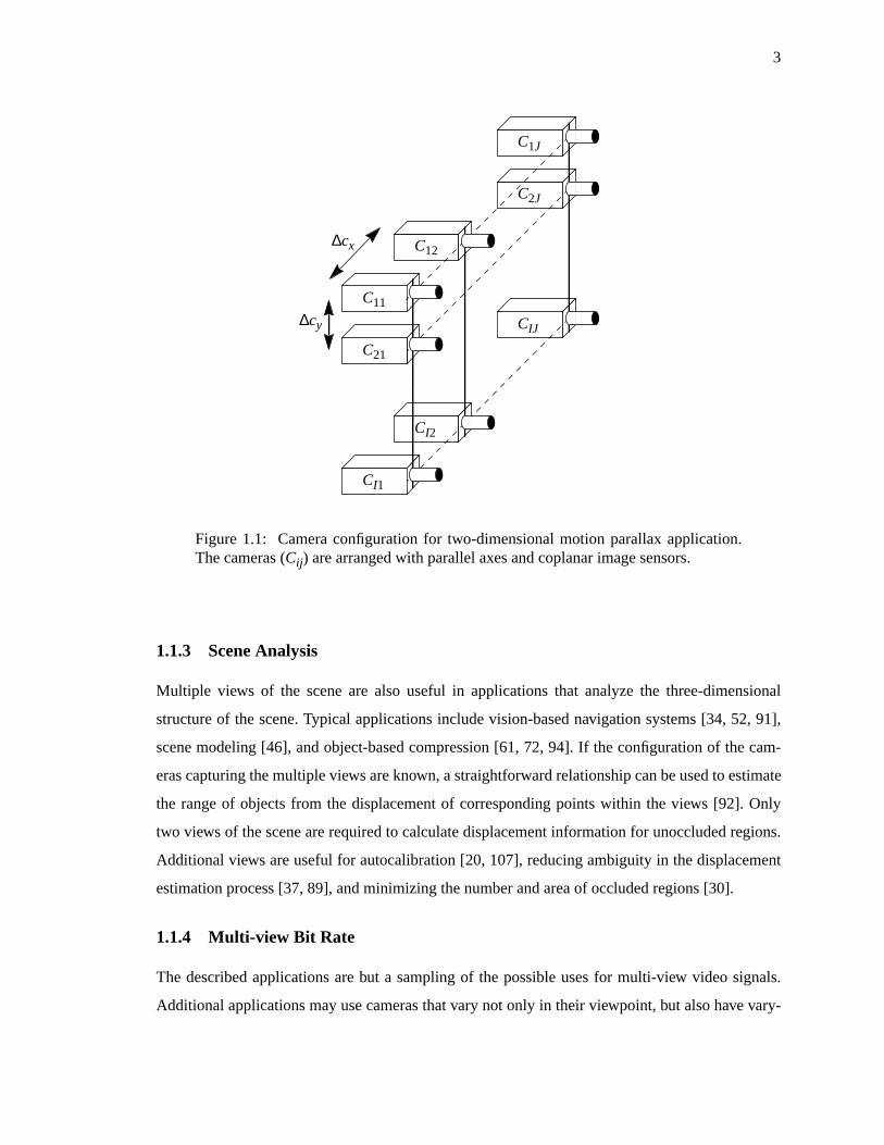
Figure 1.1: Camera configuration for two-dimensional motion parallax application. Thecameras (Cij) are arranged with parallel axes and coplanar image sensors............3
Figure 1.2: Frame-based hybrid encoder and decoder structures. ............................................7
Figure 2.1: Camera viewpoint and relationship between world-coordinates and pixellocation. ................................................................................................................19
Figure 2.2: Periodic, horizontally-spaced views, a) twenty stacked images, b) epipolar planeimage (EPI) for middle row of stacked images. ...................................................23
Figure 2.3: Camera Parameter Set A. .....................................................................................29
Figure 2.4: Camera Parameter Set B.......................................................................................30
Figure 2.5: Cement Mixer sequence, frame 50. ......................................................................33
Figure 2.6: Volleyball sequence, frame 200. ...........................................................................34
Figure 2.7: Finish Line sequence, frame 100..........................................................................35
Figure 2.8: Skater sequence, frame 175..................................................................................36
Figure 2.9: Toy Train sequence, frame 150.............................................................................37
Figure 2.10: Piano sequence, frame 50.....................................................................................38
Figure 2.11: Manege sequence, frame 25. ................................................................................39
Figure 2.12: Flower Garden sequence, frames 75 and 77. .......................................................40
Figure 3.1: ℵ4 (a) andℵ8 (b) two-dimensional, noncausal neighborhoods...........................44
Figure 3.2: Relationship between occlusion and unoccluded region displacementdiscontinuity, a) sample frames with constant displacement for background andforeground object, b) vertical component of actual displacement along middleimage column. ......................................................................................................51
Figure 4.1: Two-view scenario illustrating time-varying location of the optimal referenceframe.....................................................................................................................57
Figure 4.2: Flow-chart for adaptive reference frame selection algorithm...............................61
Figure 4.3: Three-view reference frame location scenario, a) single-step predictions, b)possible reference frames for a maximum temporal-offset of two frames...........63
Figure 4.4: Displacement vector thresholding and field reversal, a) original field, b) fieldafter SNR thresholding, c) reversed field. ............................................................66
Figure 4.5: Generation of composite displacement vector field through field addition, a) andb) single-step displacement fields, c) composite field. .........................................68
Figure 4.6: Temporal location of possible references forF(1,50.5) inFinish Line sequence.76

x
Figure 4.7: Horizontal (left-column) and vertical (right-column) displacement componentsfor Finish Line F(1,50.5), a) single-step field fromF(0,51), b) processed single-step field, c) composite field forF(0,50), d) composite field forF(1,49.5). ........77
Figure 4.8: Graphical display of estimated displacement vectors forF(1,50.5), a) referenceF(0,51), b) referenceF(1,49.5).............................................................................78
Figure 4.9: Finish Line performance for possible reference frames, a) prediction PSNR, b)total coded bits per frame. ....................................................................................79
Figure 4.10: Skater prediction PSNR comparison of fixed vs. adaptive reference frameselection for, a) entire sequence, b) last 100 frames.............................................81
Figure 5.1: Illustration of predicted-residual image correlation forManege sequence, a)originalF(0,45), b) decoded referenceF’ (1,45), c) predicted image, d) absoluteerror image. ..........................................................................................................91
Figure 5.2: Frame-based hybrid encoder and decoder structures with “prediction-directed”residual coding. ....................................................................................................97
Figure 5.3: Typical pixel neighborhoods in predicted image for the restoration of pixellocation in the residual image. Each neighborhood is denoted by theunion of shaded circles. ......................................................................................100
Figure 5.4: Vector restoration encoder and decoder structures.............................................106
Figure 5.5: PSNR vs. average rate forManege training set, a) balanced, binary trees, b)length-pruned trees. ............................................................................................115
Figure 5.6: Per-frame performance for View 0 ofManege sequence, a) PSNR, b) bits used toencode the luminance image component............................................................116
Figure 5.7: Rate-distortion comparison for View 0 ofPiano sequence, a) PSNR, b) totalcoded bits per frame. ..........................................................................................118
Figure 5.8: Rate-distortion comparison for View 1 ofPiano sequence, a) PSNR, b) totalcoded bits per frame. ..........................................................................................119
Figure 5.9: Rate-distortion comparison for View 0 ofFinish Line sequence, a) PSNR, b)total coded bits per frame. ..................................................................................120
Figure 5.10: Rate-distortion comparison for View 1 ofFinish Line sequence, a) PSNR, b)total coded bits per frame. ..................................................................................121
Figure 6.1: Multi-view system for simulated motion parallax and viewer-specified inter-camera separation, (a) functional block diagram, (b) virtual camera positions ofdesired intermediate views. ................................................................................126
Figure 6.2: Interpolated displacement vector field along epipolar line.................................129
Figure 6.3: (a) Actual displacement field, (b) estimated field with occluded (blackened) andambiguously-referenced (lightly-shaded) image regions. ..................................131
Figure 6.4: Flow-chart for improved viewpoint interpolation technique..............................138
Figure 6.5: Self-synthesis operation along single epipolar-line, (a) actual displacement field,(b)-(d) synthesis of View 0 from View 1, (e)-(g) synthesis of View 1 from View0, (h) final processed field. .................................................................................143
Figure 6.6: Inferring range information for occluded regions, (a) perspective project ofsample scene, (b) field interpolated from unoccluded regions, (c) interpolatedfield after filling occluded regions......................................................................147
u v,( )

xi
Figure 6.7: Flower Garden, (a) original frame 0, (b) original frame 3.................................159
Figure 6.8: Estimated displacement fields (horizontal component) after various processingstages. Left column: frame 0 from frame 3. Right column: frame 3 from frame 0.(a) after thresholding, border elimination and field reversal, (b) after self-synthesis of frame 0, (c) after self-synthesis of frame 3.....................................160
Figure 6.9: Occlusion localization results, (a) frame 0, (b) frame 3. ....................................161
Figure 6.10: Flower Garden frame 1, (a) original, (b) interpolated. ......................................162
Figure 6.11: Absolute frame difference for frame 1, (a) frame repetition, PSNR=15.72 dB, (b)interpolation, PSNR=28.14 dB...........................................................................163
Figure 6.12: Flower Garden frame 1, (a) interpolated without performing displacement fieldprocessing and ambiguous region selection (PSNR=24.54 dB), (b)bidirectionally-predicted from reference frames 0 and 3 using a fixed-size, block-based technique (PSNR= 28.55 dB)...................................................................164
Figure 6.13: Flower Garden frame 2, (a) original, (b) interpolated. ......................................165
Figure 6.14: Absolute frame difference for frame 2, (a) frame repetition, PSNR=15.85 dB, (b)interpolation, PSNR=28.00 dB...........................................................................166
Figure 6.15: Flower Garden frame 2, (a) interpolated without performing displacement fieldprocessing and ambiguous region selection (PSNR=24.86 dB), (b)bidirectionally-predicted from reference frames 0 and 3 using a fixed-size, block-based technique (PSNR= 28.89 dB)...................................................................167
Figure 6.16: Volleyball, (a) originalF(0,155), (b) originalF(1,155) ......................................168
Figure 6.17: Volleyball F(0.5,155), (a) interpolated using enhancements, (b) interpolatedwithout enhancements. .......................................................................................169
Figure 6.18: Cement Mixer, (a) original F(1,175), (b) original F(2,175)................................170
Figure 6.19: Cement Mixer F(1.25,175) interpolated using improved technique...................171
Figure 6.20: Cement Mixer F(1.5,175) interpolated using improved technique.....................172
Figure 6.21: Cement Mixer F(1.75,175) interpolated using improved technique...................173
Figure 6.22: Cement Mixer F(1.5,175) interpolated without displacement field processing..174
Figure 6.23: Cement Mixer F(1.5,175) interpolated using range ordering for ambiguously-referenced image regions and zero displacement occlusion filling. ...................175
Figure 6.24: Cement Mixer F(1.5,175) interpolated using unprocessed field, range orderingfor the selection of ambiguously-referenced image regions, and filling of holeswith zero displacement. ......................................................................................176
Figure 6.25: Piano, (a) originalF(0,25), (b) originalF(1,25) ................................................177
Figure 6.26: Piano F(0.5,25), (a) interpolated using improved technique, (b) interpolatedusing basic scheme. ............................................................................................178
Figure 6.27: Close-ups ofPiano frame, (a) originalF(0,25), (b) interpolatedF(0.5,25) usingimproved technique (c) interpolatedF(0.5,25) using basic interpolation scheme,(d) originalF(1,25).............................................................................................179
Figure 7.1: Complete multi-view hybrid coder structure incorporating adaptive referenceframe selection, restoration-based residual coding, and viewpoint interpolationfrom a noisy displacement vector field...............................................................183

1
Chapter 1
Introduction
We present a set of novel techniques for the efficient, predictive coding of video signals
obtained from multiple cameras positioned at arbitrary viewpoints. While multi-view video signals
can provide the benefits of added realism, selective viewing, and improved scene understanding,
an extremely large number of bits is required to describe these multidimensional signals in their
raw, uncoded form. The inherent redundancy within these signals must be fully exploited to allow
for their practical use.
The three algorithms developed in this thesis address the special characteristics of multi-view
signals and respectively improve the processes of prediction, residual encoding, and image inter-
polation within a hybrid encoder framework by: 1) adaptively selecting the best possible reference
frame, 2) exploiting the predicted-residual image correlation due to practical limitations of the pre-
diction operation, and 3) accurately interpolating occluded and ambiguously-referenced image
regions from a noisy displacement vector field. We evaluate the superiority of these algorithms on
numerous multi-view video signals through comparisons with conventional encoding techniques,
and we analyze their cost/benefit ratio in terms of increases in system complexity and storage, off-
set by rate-distortion improvements. These techniques may be performed independently of one
another or they may be concatenated into a complete multi-view system. We provide insight into
how the bit rate constraint and application for a particular signal dictate the use of one or more of
these algorithms.
1.1 Motivation
A video signal provides an enormous amount of information on the visual content of the real-
world. This information depends on both the contents of the scene and also the parameters of the
camera that generated the signal. However, a video signal obtained from a single camera can pro-

2
vide visual information about the scene from only one particular viewpoint/scale/spectral-band at
any given time instant – certain visual communication applications require more information.
Multiple views of the scene can provide the benefits of added realism, selective viewing, and
improved scene analysis. The motivation for the efficient compression of multi-view signals next
will be provided through the development of example applications that illustrate these benefits.
1.1.1 Binocular Imagery
An obvious application requiring more than one view of the scene is that of a binocular imaging
system. Binocular imagery, which, on a suitable display, precisely replicates the geometry of
human vision, is obtained from two identical cameras separated by a horizontal distance, which is
equal to the inter-ocular separation (typically 65 mm), and oriented with parallel camera axes and
coplanar image sensors [33]. By presenting the appropriate views to the corresponding left- and
right-eyes of a viewer, two slightly different perspective views of the scene are imaged on each ret-
ina. The brain then fuses these images into one view and the viewer experiences the sensation of
stereopsis, which provides added realism through improved depth perception [45, 95].
1.1.2 Motion Parallax
For further improvements in realism, the binocular imaging system can be extended to provide the
viewer with the depth cue of motion parallax [74, 99].1 Motion parallax, which provides the dis-
tinction between binocular and three-dimensional imagery, can be simulated by obtaining multi-
ple, closely-spaced views of the scene and then presenting the appropriate binocular image pair
based on the viewer’s position. Psychovisual studies of the capabilities of the human visual system
to discern variations in object displacement indicate that over ten distinct views per inter-ocular
separation are needed to ensure smooth and realistic motion parallax [51, 75].2 The camera config-
uration of a system capable of providing both horizontal and vertical motion parallax is shown in
Fig. 1.1. In this scenario, cameras are positioned on a two-dimensional grid, with camera
spacing of∆cx in the horizontal direction and∆cy in the vertical direction.
1. Motion parallax is the phenomenon whereby a change in the viewer’s position results in objectsappearing to move, with the amount of displacement inversely related to the object’s distance fromthe viewer.
2. Specifically, the required number of views depends on the depth range of the scene and the visibil-ity threshold for parallax shifts. A threshold of 1.15 min of arc was estimated experimentally in[75].
I J×
3
1.1.3 Scene Analysis
Multiple views of the scene are also useful in applications that analyze the three-dimensional
structure of the scene. Typical applications include vision-based navigation systems [34, 52, 91],
scene modeling [46], and object-based compression [61, 72, 94]. If the configuration of the cam-
eras capturing the multiple views are known, a straightforward relationship can be used to estimate
the range of objects from the displacement of corresponding points within the views [92]. Only
two views of the scene are required to calculate displacement information for unoccluded regions.
Additional views are useful for autocalibration [20, 107], reducing ambiguity in the displacement
estimation process [37, 89], and minimizing the number and area of occluded regions [30].
1.1.4 Multi-view Bit Rate
The described applications are but a sampling of the possible uses for multi-view video signals.
Additional applications may use cameras that vary not only in their viewpoint, but also have vary-
Figure 1.1: Camera configuration for two-dimensional motion parallax application.The cameras (Cij) are arranged with parallel axes and coplanar image sensors.
C11
∆cx
∆cy
C12
C21
CI1
CI2
CIJ
C1J
C2J

4
ing scale [101] and spectral bandwidth selectivity parameters [5, 35]. Regardless of their ultimate
use, it is likely that these signals will need to be transmitted and/or stored in order to be displayed
at a remote location, re-displayed at a future time, or processed off-line.
In its raw form, the bit rate for a multi-view signal is given by the simple equation,
(1.1)
For common values of 30 frames per second (fps), pixels per frame (ppf), and 24 bits
per pixel (bpp), the uncoded bit rate for a signal with three views is over bits per second
(bps). Using the digital video transmitter described in [38], a compression factor of at least 33:1 is
required to broadcast this multi-view signal in a 6 MHz channel, with a service area comparable to
the NTSC service area.
Since visual communication systems are often constrained by their transmission bandwidth
and storage requirements, it is imperative that the bit rate for multi-view signals be reduced
through the removal of redundant and irrelevant information within and between the various
views.
1.2 Problem Description
We will examine the problem of efficiently compressing multi-view video signals, where the cam-
eras are restricted to vary only in their viewpoint; i.e., all cameras have identical scale and spectral
bandwidth parameters. As a point of reference, the example applications described in Section 1.1
satisfy this constraint.
We will strive for near-term solutions, in the sense that the compression algorithms developed
or enhanced should be realizable with current, available technology suitable for mass-market pro-
duction. This goal not only attempts to limit the complexity and related cost of systems that utilize
these algorithms, but also ensures that any additional costs will be commensurate with the benefits
provided by multi-view signals. Therefore, we will remain within ahybrid encoder framework
(see Section 1.3.1), and we will develop techniques that are consistent with this methodology and
exploit the special characteristics of these signals.
We will measure the success of the algorithms developed in this thesis through the improve-
ment in rate-distortion performance over both conventional, single-view techniques applied to
each view and techniques that explicitly address multi-view signals. We will also conduct resource
bit rate # of views( ) frames per second( )× pixels per frame( )× bits per pixel( )×=
640 480×
6.6 108×
5
requirement analyses to satisfy our realizability constraint. System designers should find this cost/
benefit analysis valuable when they decide whether to implement a particular algorithm.
1.3 Related Work
This section describes work related to the problem of efficiently compressing multi-view video
signals. Often, this work has amounted to merely replicating single-view systems. The merits of
the various techniques are presented, and areas that warrant additional research are highlighted. In
particular, since we are dealing with the hybrid coder framework, the methodology and limitations
of this approach will be discussed in detail.
1.3.1 Hybrid Coders
A common method for the compression of both single- and multi-view video signals is that of a
frame-based hybrid coder. The hybrid nature of these coders is their combination of both frame-
based prediction and residual encoding, which respectively exploit redundancy between (inter) and
within (intra) frames. Interframe redundancy is due to the predictable displacement of objects
between frames, while intraframe redundancy is due to the spatial correlation of pixels. Popular
single-view implementations of hybrid coders are found in the MPEG-1, MPEG-2, H.261, and
H.263 video compression standards [1, 2, 3, 4]. Frame-based hybrid encoders view a video signal
as a set of image frames. The signal is compressed by performing intraframe coding on marker
frames, and by encoding all other frames using information from previously decoded frames. The
marker frames are used for initialization, random-access and re-synchronization purposes.
Additional views are easily incorporated into this methodology due to the frame-based
approach, where the number of frames increases linearly with the number of views. This extension
of the hybrid coder structure has been reported in numerous systems dealing with multi-view sig-
nals [15, 59, 78, 86, 87]. The frames from each view may be treated equally or an implicit ranking
may be established between the individual views. The latter approach is taken by the recently pro-
posed multi-view extension to the MPEG-2 standard, which uses the temporal-scalability option of
the standard to accommodate multiple views of the scene [77]. The MPEG-2 Multi-View Profile
(MVP) defines one view as the base layer and all additional views as enhancement layers. This
ranking is used to ensure compliance with the MPEG system-layer structure and to avoid any
restriction on the number of allowable views.

6
Frame-based hybrid encoder and decoder structures are depicted in Fig. 1.2, where the predic-
tion and residual encoding/decoding functional blocks may contain numerous lower-level opera-
tions. While these processes are highly interrelated, most multi-view techniques known to us treat
them independently. We next describe work performed on the compression of multi-view signals
with respect to the prediction and residual encoding operations, while remaining cognizant of their
interdependence. We follow this by examining techniques for removing irrelevant information
from these signals.
1.3.1.1 Frame-based Prediction
The prediction process reduces interframe redundancy by requiring only new information between
frames to be encoded. The prediction operation typically amounts to the specification of a dis-
placement model and the tracking of corresponding regions between frames.3 The degree of inter-
frame redundancy in a single-view signal is related to the temporal sampling rate, the motion of
the camera, and the motion of objects within the scene. For relatively high sampling rates and
moderate camera and object motion, the compression gain achievable from the prediction process
is quite impressive (an order of magnitude increase in the prediction peak signal-to-noise ratio
over simple frame repetition is common [31, 44]). Similar gains have been reported for multi-view
signals, where the frame-based prediction is generated from a reference frame offset in time and/or
viewpoint [5, 15, 23, 59, 86, 102]. For these systems, interframe redundancy is related not only to
the temporal sampling rate and object motion but also to the scene structure and camera configura-
tion.
For multi-view signals, the number of bits needed to describe the prediction can be reduced if
the reference frame is offset from the desired frame only in viewpoint. Since the prediction is
described by the displacement of regions between the reference and desired frame, fewer bits are
needed if the displacement range is restricted. The displacement range of corresponding points
between two views obtained at the same time instant is constrained to one-dimension, which is
referred to as the epipolar line [9, 11, 56, 92].4 Since the camera configuration is rarely known to
3. Due to their overwhelming use, we will consider only block-based (fixed and variable sized) dis-placement compensated prediction schemes in this thesis. As such, we shall interchangeably usethe terms prediction process and displacement estimation/compensation.
4. Assuming a pinhole camera model, a point in three-dimensional space will project its image at theintersection of the camera’s sensor plane with the line passing through the point and the cameralens. The relative location of the corresponding projection in another view must lie along the epipo-lar line, which is the intersection of the other camera’s sensor plane with the plane containing thetwo camera lenses and the image point.

7
Figure 1.2: Frame-based hybrid encoder and decoder structures.
FramePrediction
ResidualEncoding
Prediction description (transmit)
ResidualDecoding
Decoding description (transmit)Original image
Predicted image
Reconstructed image
+
-
+
+
Prediction description
Residual
Predicted image
Reconstructed image
Frame
+
+
ENCODER
DECODER
Decodingdescription
Frame prediction schemes:
- block-based- segmentation-based
Residual encoding schemes:- DCT, wavelet- SQ, VQ- RLE, entropy coding
Decoding
Prediction

8
the level of accuracy required to exactly specify the epipolar line, most multi-view prediction
schemes allow for some deviation in the displacement range from the 1-D constraint.
A substantial body of work has been devoted to improving the prediction performance for
multi-view signals through segmentation-based schemes, which are applicable to both single- and
multi-view signals [14, 87, 100]. These techniques begin to approach the concept of content-based
coding (see Section 1.3.3) by predicting homogeneous regions within each frame from a reference
frame, as opposed to purely pixel-based schemes, such as the ubiquitous block-based techniques.
Regions are segmented and classified based on numerous attributes, including their displacement
between frames. The standard approach for these techniques is a split-and-merge process whereby
larger-sized regions are split using a multiresolutional decomposition, and regions with similar
attributes are merged at the higher levels of resolution. The attributes may be tracked through time
to avoid the computational cost of performing the segmentation and to reduce the number of bits
needed to describe the region structures.
Superior frame predictions are possible due to the signal dependent nature of the segmenta-
tion-based algorithms: areas uniform in the selected attributes are segmented into larger-sized
regions, requiring fewer bits per pixel to describe their displacements; more bits are allotted to
detailed areas through their segmentation into smaller-sized regions. The improved prediction has
been shown to significantly reduce the number of bits needed in the residual encoding stage [14,
87, 100]. The more accurate displacement estimation afforded by these techniques also can be
used to improve displacement-compensated interpolation schemes (see Section 1.3.2). However,
segmentation-based methods are not without their faults. If the scene contains numerous, high-
detail regions, the coder’s bit rate actually may increase over pixel-based prediction schemes.
Also, the split-and-merge process is often quite heuristic and may require fine tuning to yield an
adequate segmentation. Nevertheless, segmentation-based prediction likely will be an integral por-
tion of future multi-view encoding systems.
One seemingly glaring omission in both the displacement-range-constraint and the segmenta-
tion-based-prediction bodies of work is that the reference frames used to predict the desired frame
are often heuristically chosen and pre-selected. The performance of frame-based predictors is
related to the notion of “similarity” between the desired and reference frames. For single-view sig-
nals, the most similar reference frame is generally the temporally nearest decoded frame. How-
ever, the relative location of the optimal reference frame for multi-view signals is not as
straightforward; it depends on the structure and motion of both scene objects and cameras, and it
varies as the signal evolves and progresses. The gain that would be achieved through the use of the

9
most similar reference frame is independent of the type of frame-based prediction used [64]. Puri,
et. al, allude to the effect of reference frame configuration on coding performance for stereoscopic
video in [78]; yet, they do not discuss how the optimal reference should be selected. The develop-
ment of an algorithm to overcome this shortcoming is one of the major contributions of this thesis.
1.3.1.2 Residual Encoding
Ideally, the difference (residual) between the original and predicted images would be spatially-
uncorrelated. In fact, the underlying content of the original image can always be seen in the resid-
ual image, and traditional still-image compression techniques then can be applied to exploit this
correlation. The residual encoder may include numerous operations, such as: the transformation of
the residual image data to a generalized frequency domain (DCT [18] and wavelet transformations
[49]), and the application of both lossy (scalar and vector quantization [32]) and lossless (run-
length and entropy coding [42]) compression techniques. The choice of which technique(s) to use
depends on the bit rate, complexity and reconstruction fidelity constraints of the system along with
the signal content.
In most hybrid coders, the majority of the bits needed to describe the coded signal are con-
sumed by the residual encoding process (for a high fidelity coded sequence, the residual coding
may require over 90% of the total bit rate). The exact number of bits required to reconstruct the
original image to a desired level of quality depends on the accuracy of the prediction and the rate-
distortion characteristics of the residual encoder. Due to the feedback nature of the hybrid coder,
this relationship also holds in the opposite direction; i.e., prediction performance is related to the
quality of the reconstructed image.
The majority of work dealing with the residual encoding process for multi-view signals has
amounted to: 1) generating a superior prediction to limit the number of bits needed to describe the
residual image (see Section 1.3.1.1), and/or 2) performing more severe, lossy compression on indi-
vidual views that are considered less subjectively-important than other views (see Section 1.3.1.3).
Even with improvements in the prediction process, it is unlikely that a system capable of yielding
“perfect” frame predictions, in the sense that the residual image contains only irrelevant informa-
tion, will be obtainable. Therefore, we feel that further work on improving the residual encoding
process is needed to adequately reduce the extremely large bit rates of multi-view video signals.
A possible area for improvement becomes apparent when the residual encoder model is exam-
ined in detail. One universal characteristic of all residual encoding schemes known to the author is
that the residual image is operated upon independently of any knowledge of the predicted image.

10
This approach is based on the model that the original image consists of both a predictable portion
and an unpredictable, white-noise component [26]. The prediction operation is assumed to exactly
yield the predictable information of the original image and the residual image merely contains the
white-noise process. Therefore, the residual and predicted images are uncorrelated and no coding
gain is possible through the use of information available in the predicted image. However, due to
the bit rate and complexity constraints imposed on the prediction process and the non-stationarity
of the image data, this model becomes invalid: substantial correlation exists between the predicted
and residual images. This is particularly true when the coder operates in low bit rate regions [29].
A substantial contribution of this thesis is the development of a novel coder model that
exploits this correlation, due to the practical constraints on the prediction process, to achieve supe-
rior rate-distortion performance over traditional residual encoders. A technique similar to our solu-
tion was reported independently by Richardson in [84]; however, this work was concerned with the
problem of restoring a degraded image using only a model of the degradation process and did not
address the coding problem.
1.3.1.3 Irrelevancy Reduction
Irrelevancy reduction is the final form of information reduction in hybrid coders that will be exam-
ined. The classification of information as being irrelevant depends on the use of the information.
When video is to be viewed by a human observer, characteristics of the human visual system
(HVS) can be exploited to remove information that is imperceptible to the viewer. For single-view
systems, irrelevancy reduction typically amounts to performing spatial- and temporal-frequency
dependent quantization. Example techniques include devoting more bits to lower spatial-frequency
components of the signal, subsampling the chrominance information, and relaxing fidelity require-
ments for high-motion regions [60].
These methods may be applied to multi-view signals intended for viewing by a human
observer. Also, binocular systems often exploit the singularity-of-vision property of the HVS to
remove irrelevant information [22]. In binocular vision, one eye is dominant over the other eye –
artifacts viewed by the non-dominant eye will be masked by the dominant eye. This feature allows
for a non-symmetric allocation of bits between the two views; i.e., one view is compressed much
more coarsely than the other view. Problems with this approach arise since not all viewers have the
same dominant eye. Also, it is unclear how more than two views would be ranked, and whether a
classification and subsequent differential compression of multiple views is justifiable. Therefore,

11
we wish to develop multi-view algorithms that do not rely on the singularity-of-vision property to
achieve an improved compression ratio.
1.3.2 Displacement-compensated View Interpolation
A related technique for the compression of multi-view video signals is that of intermediate view
synthesis or interpolation. Here, a minimal set of views that represent the structure of the scene are
coded using a conventional hybrid encoder. Additional views, interior to the given views, are then
interpolated at the decoder by mapping pixel intensities based on the displacement of image
regions. Viewpoint interpolation is important in numerous applications, such as the system capable
of simulating horizontal and vertical motion parallax, which would require an excessive camera
complexity and bit rate if all views were captured, encoded and transmitted. It would be much
more efficient to capture and transmit only the views on the four corners of the two-dimensional
grid, and then to synthesize the other views at the decoder.
Numerous techniques for the synthesis of intermediate views have been reported in the litera-
ture. A common approach is through the generation of epipolar plane images (EPI) [30, 40, 47].
The EPI-based techniques use multiple, closely-spaced views of the scene to minimize the occur-
rence of occlusion and reduce errors in the displacement estimation process; however, if an accu-
rate model of the displacement of objects between views is known, the generation of multiple
views amounts to oversampling the scene and is inherently redundant. The other class of tech-
niques for the synthesis of intermediate views is that of displacement-compensated view interpola-
tion, which is closely related to motion-compensated interpolation of single-view signals for frame
rate conversion, de-interlacing and frame skipping [13, 41, 47, 48, 83, 93]. Here, the intermediate
view is synthesized by estimating the displacement of regions between two views and linearly
scaling this displacement based on the relative viewpoint of the desired view between two given
views. This operation is straightforward and accurate for unoccluded regions where the exact dis-
placement is known. The performance of displacement-compensated interpolation schemes
degrades abruptly when a region is visible in only one view (occluded) and when displacement
estimation errors occur [63]. Techniques for handling occlusions in single-view signals are pro-
vided in [83] and [93]. However, these methods are not applicable to multi-view imagery, and they
do not achieve an adequate delineation of occlusion borders to avoid a subsequent residual encod-
ing stage for image pairs with relatively large displacement ranges.
Since we wish to eliminate the generation and transmission of the interior views for the com-
pression of multi-view signals, we do not have the luxury of performing residual encoding to

12
reconstruct the desired view if the interpolation process yields an unsatisfactory image. We also
wish to synthesize intermediate viewpoints using only the information available from the decoding
of a representative set of exterior views. We address the problem of improving the interpolation
performance for occluded and ambiguously-referenced regions from a noisy displacement vector
field by using knowledge of the camera configuration and the displacement estimation process.
The development of this enhancement, which provides improved interpolation for these “difficult-
to-synthesize” regions, is the final contribution of this thesis.
1.3.3 Content-based Coders
A recent trend in video compression algorithms is the shift from frame-based methodologies to
techniques that treat video as a combination of visual objects. In its simplest form, content, or
object, based compression entails the segmentation of image frames into “objects” that have some
common attributes or features, which may or may not correspond to physical objects (see Section
1.3.1.1). More sophisticated content-based coders attempt to decompose the video signal into real-
world objects. Once the signal has been decomposed, the object models are sent to the decoder and
the video signal is reconstructed from a script describing how the objects evolve as the signal
progresses. Content-based coding is at the core of the MPEG-4 video compression standard cur-
rently under development, which contains a provision for the compression of multiple, concurrent
views of the scene [81].
This object-based methodology efficiently handles multi-view signals since an object visible
in separate views can be represented compactly as a single object, and the various perspective
views can by synthesized from the object model and knowledge of the camera viewpoints. This
capability also can be used to generate views from “virtual” viewpoints, perform content-based
retrieval, and actually alter the content and evolution of the video signal [81].
Unfortunately, the availability of systems employing content-based compression is limited due
to problems with robustness and complexity; user-intervention is often required to obtain subjec-
tively-acceptable coded video and the operations of object detection, segmentation, and tracking
are time-consuming and do not easily facilitate parallel implementations, as do the rote frame-
based techniques. Also, object-based systems do not scale well to multiple objects.
We take the stance that, while content-based coders may eventually provide a very efficient
representation of multi-view video signals, real-time and robust systems are still quite a few years
away from reality. To improve upon current multi-view visual communication systems employing
hybrid coders and also future content-based coders, we will address the problems of: 1) selecting
13
the best possible reference frame for the prediction/segmentation process, 2) fully exploiting the
residual-predicted image correlation to improve the performance of the residual encoder, responsi-
ble for handling situations when the prediction/segmentation process is imperfect, and 3) interpo-
lating virtual viewpoints based on noisy displacement vector fields obtained from frame-based
displacement estimation techniques.
1.4 Contributions
This section details the contributions of this thesis for the concurrent compression of multiple,
interrelated video signals. For clarity, the contributions are separated into the scope of the specific
algorithms presented. Individually, these algorithms are valuable video compression tools;
together, they represent a complete and efficient methodology for the compression of multi-view
signals.5
1.4.1 Optimal Reference Frame Selection
We present a new algorithm that adaptively selects the best possible reference frame for the predic-
tive coding of multi-view video signals, based on estimated occlusion percentage with the desired
frame. We illustrate the effect of occlusion on prediction performance, and develop the underlying
principle that relates occlusion and the discontinuity between displacement vectors of adjacent,
unoccluded image regions. We provide a method to estimate the relative amount of occlusion
between two frames from the variance of a composite displacement vector field. Single-step dis-
placement fields are combined to generate the composite fields, which eliminates the computation-
ally costly process of displacement estimation for each candidate reference frame. The reference
frame with minimum occlusion (maximum similarity) then is used in the prediction of the desired
frame.
The performance increase obtainable from using this algorithm is obviously signal-dependent.
When compared with non-adaptive techniques, the adaptive algorithm achieved up to 4 dB
improvement in frame prediction performance and required 10-30% fewer bits for the residual
encoding process, for the set of multi-view signals examined in this thesis. These gains are
obtained with acceptable complexity and storage costs.
5. These algorithms have been implemented in a software simulation capable of performing any com-bination of the described techniques, along with other conventional schemes. All experimentalresults were obtained from this simulation.

14
1.4.2 Restoration-based Residual Coding
We develop a novel class of residual coders that adaptively exploits the non-trivial correlation
between the predicted and residual images. This concept represents a significant addition to the
theory of predictive coding. We present a stochastic model of the multi-view video signal and
illustrate how the practical constraints imposed on the prediction process and the non-stationarity
of the signal preclude the residual image from being uncorrelated with the predicted image. The
vector restoration coder involves the application of optimal operations to predicted image blocks
(vectors) with the goal of restoring the original image block. Compression is achieved by only
transmitting the index of the restoration operation from a codebook of operations for each pre-
dicted image block.
Vector quantization is shown to be a special, and generally sub-optimal, case of vector restora-
tion. In fact, in the unlikely event that the predicted and residual images are uncorrelated, these
techniques are equivalent. By using the vector restoration coder, the bit rates for the signals exam-
ined were reduced by 15% when compared to a vector quantization implementation. Similar,
although not as impressive, improvements were observed over DCT-based residual coders. How-
ever, the restoration-based encoder requires a substantial increase in storage and complexity costs
over the VQ and DCT approaches, and is thus most suitable for applications with severe bit-rate
constraints.
1.4.3 Interpolation from a Noisy Displacement Vector Field
We enhance displacement-compensated interpolation algorithms by accurately handling displace-
ment estimations errors, occlusions, and ambiguously-referenced regions. We examine the dis-
placement estimation process and illustrate the causes of estimation errors. We detect occluded
regions and displacement estimation errors through a displacement estimation confidence mea-
sure. The location of displacement discontinuities, or equivalently occlusions, are finely delineated
through the process ofself-synthesis, which checks the accuracy of the displacement estimates by
interpolating the given views from each other. Scene assumptions and knowledge of the camera
configuration of the given views are used to fill-in displacement information for occluded regions.
The complete and processed displacement vector field then can be used in a standard displace-
ment-compensated interpolation algorithm to generate the desired view.
This enhancement has been used in the interpolation of numerous multi-view images. The
effect of displacement estimation errors were significantly reduced and occluded regions were
accurately synthesized, as evidenced by comparisons with actual intermediate views. Multiple

15
interpolated views have been displayed on a multi-view binocular imaging system, with subjec-
tively effective motion parallax.
1.5 Thesis Outline
We begin Chapter 2 by providing a formal definition of single-view video signals and extend this
notion to multi-view systems. We then discuss the relative difficulty in coding multi-view signals
with arbitrary viewpoints as compared to those with periodic camera parameters. Finally, we pro-
vide the quantitative cost measures and describe the multi-view video signals used in the analysis
of the algorithms developed throughout the remainder of this thesis.
The theoretical basis for the multi-view compression algorithms developed in this thesis is pre-
sented in Chapter 3. We model image intensities in terms of a non-stationary, Gauss-Markov pro-
cess. The non-stationarity is due to spatiotemporally-varying correlation coefficients, which model
variations in lighting and camera pick-up parameters both within and between frames. We assume
a rigid-body, translational displacement model for scene objects, and we make numerous observa-
tions on the geometrical constraints of displacement vector fields. Fundamental results are the rela-
tionship between displacement discontinuity and occlusions and the use of a displacement
confidence measure to eliminate displacement estimates that contradict the established geometri-
cal constraints.
In Chapter 4, we present our solution to the problem of selecting the reference frame that
yields optimum prediction performance. We first provide motivation for the adaptive selection of
the best possible reference frame. We then describe the selection algorithm in detail, which is
based on the amount of occlusion between the desired and reference frames. This approach is
compared with other possible reference frame selection methods, and the experimental results
demonstrate the rate-distortion superiority of our algorithm.
We develop the novel class of restoration-based residual coders in Chapter 5. We begin by
illustrating how the practical constraints on the frame-based prediction process result in a sub-opti-
mal predicted image, which in turn can be used to improve the residual encoding process. We then
describe the vector restoration coder in detail, which is very similar in implementation to a vector
quantizer (VQ). We extend the common tree-structured, multi-stage, and variable rate VQ tech-
niques to the basic restoration-based coder. This technique is compared with VQ and DCT-based
methods through theoretical and experimental analysis.
In Chapter 6, we provide our method for accurately interpolating intermediate views from a
decoded image pair by considering occluded and ambiguous regions. We briefly discuss the simple

16
process of interpolation for unoccluded regions and develop assumptions that allow for range
information of occluded regions to be inferred from adjacent unoccluded regions. We use numer-
ous techniques developed in Chapter 4 to eliminate poor displacement estimates, and we refine the
estimates further by interpolating the given image pair. The performance of this enhancement is
evaluated through informal subjective assessments using a multi-view display system and through
quantitative comparisons when the true intermediate views are available.
Conclusions and areas for future work are described in Chapter 7. We also discuss the relative
contributions of these algorithms, and provide insight into how and when these techniques should
be combined into a complete multi-view encoder/decoder system.

17
Chapter 2
Multi-view Video Signals
In this chapter, we extend the common notion of a video signal to include multiple, concurrent
views of the scene. We then define arbitrary multi-view signals and illustrate the relative difficulty
experienced in coding these signals compared to those with quasi-periodic camera parameters.
Finally, we provide the quantitative measures used in the cost/benefit analysis of the algorithms
developed, and describe the content and camera parameters of the multi-view signals used
throughout this thesis.
2.1 Extension from Single-view Signals
A single-view video signal is generated by an optical sensor that samples the electromagnetic radi-
ation of a scene on both a two-dimensional, spatial grid and also temporally. The three-dimen-
sional single-view video signal (SVS) can be decomposed into a sequence of image frames, which
are ideally the perspective projection of the visual information of the scene through the camera
lens and onto the camera sensor at specific time instants. The notation for an SVS, consisting ofN
frames, is given by,
, (2.1)
wheren is the frame index,T is the temporal sampling period, and is thenth frame in the
sequence. Each frame contains the complete set of samples captured on the image sensor plane,
and is denoted by,
, and (2.2)
SVS F nT( )= n 0 … N 1–, ,{ }∈∀
F nT( )
F nT( ) I u v nT, ,( )= u∀ 0 … U 1–, ,{ }∈ v∀ 0 … V 1–, ,{ }∈

18
where is the picture element (pixel) at location within the pixel frame.
The content of the video signal is related to a set of parameters that uniquely describe the cam-
era that generated the signal. These parameters provide the camera viewpoint, scale, and spectral
bandwidth sensitivity. The variation of these parameters between temporal samples can provide
knowledge of interframe correlation. For example, if the camera alters its viewpoint by panning
across the scene, the displacement of all motionless objects between frames is constant over the
entire frame and is directly proportional to the pan-angle. However, due to the relative difficulty in
quantifying the parameter variations over time, most single-view compression techniques neglect
the effect of these parameters; the camera parameters are assumed to be static and the evolution of
the signal content is assumed to be the result of object motion.1
We now extend our notion of video signals to include signals obtained from the parallelization
of multiple SVS’s, which we refer to as multi-view video signals (MVS). The cameras that gener-
ated these distinct views obviously must have varied in at least one camera parameter. The relative
camera parameters can be used to index the views and to provide knowledge of the inter-view cor-
relation. Therefore, we will incorporate the relevant parameters into the notation of multi-view
video signals. We assume that the relative values are constant throughout the duration of the video
signal, and that the pertinent parameters are calibrated initially. These assumptions eliminate the
difficult process of tracking the absolute camera parameters through time.
Since we have restricted ourselves to the compression of multi-view video signals with distinct
viewpoints, we fix and, subsequently, disregard all other camera parameters in the notation for
MVS’s. For simplicity, we assume a pinhole camera lens model and that the camera axis is perpen-
dicular to the plane of the camera sensor. Applying these constraints, the camera model and view-
point are specified by three triplets that respectively denote: 1) the position of the camera lens,c,
2) a point,p, that lies on both the sensor plane and the camera axis, and 3) the endpoint,e, of a unit
vector that lies on the sensor plane, is parallel with theu-axis of the image sensor and whose origin
is p.2 The line defined by pointsp andc forms the camera axis, which specifies camera pan and tilt.
The focal length of the camera is . The roll vector, given by , provides the rota-
tion of the camera about its axis. The relationship between these points and the mapping between
3-D world- and 2-D image-coordinates are illustrated in Fig. 2.1.
1. See [104] for a description of techniques that consider the effect of global camera motion.
2. It should be noted that the pointp need not, and sometimes should not, lie at the center of the imagesensor plane. Offsets from the center are useful in binocular imaging applications to provide geo-metrically-correct stereo-vision [33].
I u v nT, ,( ) u v,( ) U V×
f p c–= e p–

19
c
e
pCamera axis
x
y
z
Figure 2.1: Camera viewpoint and relationship between world-coordinates and pixellocation.
Sensor plane
pixel (uo
,vo)
uovo
(xo,yo,zo)
Roll vecto
r
v
u

20
Due to the constraint on the camera axis being perpendicular to the sensor plane, only six
parameters are needed to completely describe the camera viewpoint.3 We distinguish each view
within an MVS by these parameters and define the viewpoint matrix of themth-indexed view as,
(2.3)
where , , and respectively denote the tilt, pan, and roll angles of the camera about its lens,
and are related to the three triplets of the camera model.
Instead of denoting each view by its absolute viewpoint parameters, we specify a reference
viewpoint matrix and express all other matrices in the MVS with respect to this reference. By con-
vention, we use as the reference viewpoint matrix. We then define an orthonormal, right-
handed coordinate system ( ) for the 0th-indexed view, whose origin is located at , positive
z-axis is coincident with the camera axis pointing away from the sensor plane, and positivex-axis
is parallel with, and in the direction of, the roll vector. Expressed in terms of this coordinate sys-
tem, reduces to the null-matrix.
All other viewpoint matrices in the MVS are expressed in terms of by,
(2.4)
where is the differential viewpoint matrix of themth view with respect to the 0th view. The
differential viewpoint matrices may be interpreted as the parameters necessary to convert a point
expressed in themth camera’s coordinate system to a point in ; the first column vector specifies
the translation vector and the second column vector specifies the angles of the 3-D rotation matrix.
Finally, since it is often difficult to capture multi-view signals with synchronized temporal
sampling, we allow for a possible phase offset between the individual views in our notation. We
3. These six parameters do not include the camera focal length, which is needed for the mapping from3-D to 2-D coordinates. Again, since we have fixed the scale between views, we omit the focallength from our viewpoint parameter set.
Φm c Θ
cx θx
cy θy
cz θz
= =
θx θy θz
Φ0
RC0c0
Φ0
Φ0
Φm Φ0 ∆Φm+=
∆Φm
RC0

21
define the scalar as the relative temporal sampling offset of themth-indexed with respect to
the 0th-view, where and . The complete notation for an MVS, withM views,
then is obtained by extending Eq. (2.1) to include the differential viewpoints matrices and the
phase offset:
, and (2.5)
In a similar manner, individual frames within an MVS are denoted by incorporating these parame-
ters into Eq. (2.2). For simplicity, we often will denote the individual frames within the multi-view
signal by its viewpoint and temporal indices as . A fractional value for the temporal index
(n) indicates the frame’s phase offset; e.g., is the 23rd frame in View 1 captured at
. The differential viewpoint matrices indicate the degree of inter-view correlation and
the possible range of corresponding points with the various views.4
2.2 Arbitrary Viewpoints
In this thesis, we are concerned with the compression of multi-view video signals witharbitrary
viewpoints. We next define arbitrary viewpoints and discuss our motivation for restricting our
focus to this class of signals.
Arbitrary multi-view signals are most easily defined through their antonym: the class of multi-
view signals that contain a subset of at least three views whose viewpoint parameters vary in a
quasi-periodic manner. The differential viewpoint matrices for these non-arbitrary views are given
by,
(2.6)
where is the fundamental sampling period, and is a scalar function that allows for an
irregular periodic variation of the viewpoint parameters. In the simplest case, and the
4. A complete derivation of the conversion between coordinate systems and the transformation from3-D world- to 2-D image-coordinates can be found in [27].
∆tm
∆t0 0= ∆tm T<
MVS F ∆Φm nT ∆tm+,( )= m 0 … M, ,{ }∈∀ n 0 … N 1–, ,{ }∈∀
F m n,( )
F 1 23.5,( )
t 23.5T=
∆Φm q m( )∆Φ=
∆Φ q m( )
q m( ) m=

22
viewpoints possess a strict periodicity. We define the two exterior views of periodic MVS’s as the
views where is at an extremum; all other views are classified as interior views.
The majority of prior research on the compression of more than two views has dealt with non-
arbitrary viewpoints with zero phase offset [7, 30, 40, 47]. These periodic signals require a very
high camera complexity to generate the multitude of views, and they possess a simple relationship
between the interior and exterior views. If the two exterior views have some overlap in their view-
ing areas and the interior views do not contain any regions occluded from both exterior views, the
interior views contain completely redundant information that is readily extracted from the exterior
views. We can best illustrate this relationship between the interior and exterior views of non-arbi-
trary multi-view signals by re-visiting our motion parallax application (Section 1.1.2).
Assuming that we only are interested in providing the viewer with simulated horizontal
motion parallax, we require multiple, closely-spaced views whose differential viewpoint matrices
are given by,
(2.7)
Since the viewpoints only vary in their horizontal position, the displacement of corresponding
points is restricted to lie along theu-axis of the image frame. A three-dimensional structure of
twenty images, obtained from such a setup with a camera spacing of 5 mm, is shown in Fig. 2.2a.
A horizontal slice through the middle of this structure is shown in Fig. 2.2b. This slice contains the
middle row of each image and is commonly referred to as an epipolar plane image (EPI).
The EPI consists of a set of intersecting parallelograms, which represent the displacement of
scene objects through the various views. An object becomes occluded when its parallelogram is
intersected by another object’s parallelogram. Since only two corner locations and the slope of
each parallelogram are needed to completely describe the EPI from the given exterior views’ rows,
the interior rows can be encoded very efficiently. Further compression can be achieved, for the
entire set of views, by exploiting the continuity relationship between neighboring epipolar plane
images.
Other periodic variations of the viewpoint parameters result in similar structures with high
degrees of redundancy. While the task of extracting the information to efficiently encode these
structures is non-trivial, we feel that the high compression ratios often reported for non-arbitrary
q m( )
∆Φm m∆cx 0
0 0
0 0
=

23
u
v
m
a.
b.
m
0
19
Figure 2.2: Periodic, horizontally-spaced views, a) twenty stacked images, b) epipolarplane image (EPI) for middle row of stacked images.
u
Views
EPI row

24
viewpoints are obtained by essentially oversampling the scene [7, 30, 40, 47]. To avoid the genera-
tion and compression of the inherently redundant interior views, we wish to capture and encode
only the exterior views and to accurately interpolate the interior views. Our desire to only use the
exterior views is the basis of our focus on arbitrary multi-view signals.
This discussion on arbitrary viewpoints notwithstanding, we will assume that the viewpoints
of the MVS that we wish to encode have sufficient overlap with one another to ensure a certain
degree of correlation between views. This assumption is consistent with the notion of single-view
video signals, where the typical frame rate of 30 Hz results in temporally-adjacent frames to be
highly similar. While applications of multi-view signals with non-overlapping viewpoints can be
construed, the degree of compression achieved by using the knowledge of all views available most
likely will be equivalent to that which would be obtained if the views were compressed indepen-
dently. Also, displacement information between views cannot be obtained for such a situation, and
interpolation of the interior views becomes impossible.
2.3 Cost Measures
The underlying goal of any compression algorithm is the minimization of the costs associated with
the transmission and/or storage of the signal through the exploitation of both redundant and irrele-
vant information. In video compression, we desire to reduce both the coded signal’s transmission
bit rate and the distortion of the reconstructed imagery from its original form. These costs obvi-
ously are inversely related and cannot be minimized simultaneously; for a particular compression
technique, a reduction in the bit rate will cause an increase in the image distortion, and vice versa.
It is customary to evaluate various compression techniques either by fixing one cost and compar-
ing the free cost, or by comparing an overall cost function that weights the contribution of the rate
and distortion. These weights are obtained from implicit knowledge of the relative importance of
each cost.
In our cost/benefit analysis of the techniques developed in this thesis, we are interested in not
only rate and distortion, but also the costs associated with the complexity and storage requirements
of each algorithm. Complexity and storage costs are valuable for evaluating the realizability of an
algorithm; e.g., if a technique can achieve some optimum rate-distortion performance but it
requires an excessive amount of time to yield this result, the algorithm has no practical use.

25
The overall cost function that we will use to evaluate techniques for the compression of multi-
view signals is a linear combination of the coded bit rate (R), image distortion (D), algorithm com-
plexity (C), and memory storage requirement (S), and is given by,
(2.8)
where each cost is weighted by its respective , with by our convention.5 To facilitate
comparison, we will often fix either the rate or distortion of a particular multi-view signal for each
technique analyzed and examine the other costs. We next provide our definitions for the rate, dis-
tortion, complexity, and storage costs.
2.3.1 Bit Rate
Bit rate is defined simply as the average number of bits per second needed to represent the com-
pressed video signal at its temporal frame rate. We also will use the number of bits per pixel and
bits per frame as measures of coded bit rate.
2.3.2 Distortion
Distortion is inversely related to the fidelity, or quality, of the decoded images. By definition of
lossy compression techniques, some form of distortion between the original and reconstructed
images will always be present. The evaluation of distortion should be related to the application of
the imagery; for visual communication systems, distortion ideally would be related to the percep-
tual capability of the human visual system. However, we know of no widely-accepted distortion
measure that provides a quantitative result that coincides with subjective image quality. We will
thus use the often-criticized class of distortion measures that calculate the Lp-norm between the
intensity values of the original and reconstructed images [42]. These measures are easily calcu-
lated and allow for direct comparisons with other research results.
In its most basic form, we define distortion as,
(2.9)
5. Since the relative values of these weights are system dependent, we leave their assignment to sys-tem designers.
J R λDD λCC λ+SS+ +=
λi λR 1=
D1A--- I u v,( ) I u v,( )–
p
u v A∈,∀∑=

26
where is the pixel intensity of the decoded image andA is the image area in pixels. Com-
mon variations of this distortion measure are the mean-absolute-difference (MAD, ) and
the mean-square-error (MSE, ). While we have presented distortion as a measure over the
entire image frame, we will often calculate the distortion of an image region by limiting the area
over which the summing takes place.
The literature often quotes the signal-to-noise ratio (SNR) as a measure of image quality. The
SNR of a reconstructed image is given by,
(2.10)
(2.11)
(2.12)
where and respectively denote the variance and mean of the original image’s intensity.
The final distortion measure that we will use is referred to as the peak-signal-to-noise ratio
(PSNR), which is obtained by substituting the peak-to-peak intensity range (e.g., 255 for 8-bit
images) forσ in Eq. (2.10).
2.3.3 Complexity
The complexity of an algorithm is defined as the number of both fixed- and floating-point opera-
tions required to perform its functions. Due to the difficulty in exactly calculating these quantities,
we will mainly be interested in the portions of an algorithm that require looping and repeated
manipulation of image data. We will express complexity in terms of the number of operations per
pixel, and we will provide complexity costs for both the encoder and decoder, since the algorithms
presented are not symmetric.
2.3.4 Storage
The storage cost is defined as the number of bytes needed to store the data sets associated with an
algorithm. This includes both frame memory and any other relatively large structures, such as
I u v,( )
p 1=
p 2=
SNR (dB) 10 log10σ2
MSE------------
=
σ2 1A--- I u v,( )[ ]2
u v A∈,∀∑
µ2–=
µ 1A--- I u v,( )
u v A∈,∀∑=
σ2 µ

27
look-up tables and codebooks, used in the compression of the image data. Again, due to the asym-
metric nature of the algorithms examined, we will provide storage costs for both encoder and
decoder structures.
2.4 Multi-view Sequence Descriptions
This section describes the multi-view video sequences used to analyze the performance of the var-
ious algorithms developed in this thesis. We next provide the camera parameters and a brief over-
view of the content of these signals. Each sequence was captured in YUV 4:2:0 format with 8-bit
accuracy for each pixel component; the luminance and two color components were treated sepa-
rately and the color components were subsampled by a factor of two in both the horizontal and
vertical image directions. Unless specified, all sequences were captured by the author. The
sequence highlights are included in Table 2.1.
The camera parameter sets labelled A and B describe the camera configurations and temporal
sampling structures of the various sequences, and are illustrated in Figs. 2.3 and 2.4, respectively.
The viewpoint index for each view corresponds to the appropriate camera number in these figures.
The multiple time axes in these diagrams represent the temporal sampling of the scene for each
view within the MVS. The black squares are the relative temporal locations of frames, and the
dashed-lines that intersect the time axes indicate constant temporal values.
2.4.1 Cement Mixer Sequence
The Cement Mixer6 sequence was obtained using three, horizontally-spaced cameras with syn-
chronized temporal samples. The focal lengths of both cameras were 50 mm, and the camera spac-
ing was fixed at 65 mm, resulting in the differential viewpoint matrices:
, (2.13)
While these viewpoints meet our criteria for periodic multi-view signals, we use this sequence
since the three views have a relatively large spacing that precludes the interior view from being
6. The image frames in this sequence were manually shifted and cropped once per-sequence to ensurea reasonable amount of overlap between inter-view frames and subjectively-pleasing stereoscopy.
∆Φm m∆cx 0
0 0
0 0
= m 0 1 2, ,=

28
SequenceName
Numberof Views
Parameter Set
Duration(seconds)
FrameRate (Hz)
FrameResolution
Cement Mixer 3 A 7 30 544 x 480
Volleyball 2 B 8 30 640 x 240
Finish Line 2 B 9 30 640 x 240
Skater 2 B 10 30 640 x 240
Toy Train 2 B 6 50 720 x 288
Piano 2 B 2 50 720 x 288
Manege 2 B 1 50 720 x 288
Flower Garden 1 N/A 5 30 352 x 240
Table 2.1: Sequence highlights

29
entirely redundant. The camera configuration and temporal sampling structure for this signal are
shown in Fig. 2.3.
The content of this sequence includes a foreground tree, two parked cars, and a large cement
truck in the background. The cameras exhibit no camera motion. The majority of the motion in the
sequence is the slow rotation of the barrel of the cement truck, which contains lettering. Two
pedestrians walk across the scene from right-to-left. Spatially-adjacent views possess approxi-
mately 15% occlusion.
The foci of the individual views were poorly aligned, resulting in a large variation in the object
plane that was in focus for the frames within View 0 compared to the other two views. A sample
frame from each of the three views is shown in Fig. 2.5.
2.4.2 Volleyball Sequence
The Volleyball sequence consists of two views obtained by horizontally-displaced cameras with
parallel axes and coplanar image sensors. The viewpoint spacing was fixed at 160 mm and each
camera had a focal length of 50 mm, such that:
(2.14)
The temporal sampling of the two cameras was synchronized such that . The parameter
set for this sequence is shown in Fig. 2.4.
C1
C0
C2
0 T 2T
t
t
Camera configuration Temporal sampling
t
3T 4T 5T
∆cx
Figure 2.3: Camera Parameter Set A.
∆cx
∆Φ1
∆cx 0
0 0
0 0
=
∆t1 0=

30
The scene is composed of a group of individuals engaged in a game of volleyball on a back-
ground of grass. The majority of the objects in the scene are located quite a distance away from the
camera pair, resulting in a relatively small amount of inter-view occlusion. The camera pair exhib-
its random motion as the game progresses. Two frames from this sequence are provided in Fig. 2.6.
2.4.3 Finish Line Sequence
TheFinish Line sequence was captured using a commercial binocular-camera. The original cam-
era configuration was modified to ensure parallel camera axes and coplanar image sensors. The
two viewpoints differed by a constant offset of 50 mm along thex-axis. The separate views were
recorded using the field sequential characteristic of the camera, which resulted in a phase offset of
one-half the frame period ( second) between identically-indexed frames within the
two views. The camera configuration and temporal sampling structure of this signal are illustrated
in Fig. 2.4
The scene is composed of a crowd watching the end of an outdoor racing event. The people in
the scene exhibit moderate motion and the camera performs a slow, bidirectional pan. Although
the viewpoints vary by only 50 mm along and the cameras had a focal length of 9.5 mm, the prox-
imity of the people in the scene to the cameras results in a large degree of inter-view occlusion. A
sample frame from each view is shown in Fig. 2.8, where the images have been scaled by one-half
in the horizontal direction to ensure a realistic aspect ratio.
∆t1T2--- 1
60------= =
C0
C1
0 T 2T
t
t
Camera configuration Temporal sampling
Figure 2.4: Camera Parameter Set B.
∆cx
∆t1

31
2.4.4 Skater Sequence
The identical camera setup of the previous sequence was used to capture theSkater two-view sig-
nal. The sequence is composed of a quadrangle of university buildings in the background. The
camera pair follows the motion of an in-line skater as he traverses horizontally across the scene.
The cameras exhibit a rapid pan resulting in a moderate degree of intra-view occlusion on the
image frame borders. The pan rate varies greatly throughout the sequence and eventually the cam-
eras stop moving. The 175th frame from each view is shown in Fig. 2.8.
2.4.5 Toy Train Sequence
TheToy Train7 sequence was captured using a binocular camera with the same basic camera con-
figuration and temporal sampling structure as shown in Fig. 2.4. The cameras were separated by a
horizontal distance of 87.5 mm, had focal lengths of 40 mm, and a zero phase offset.
The scene consists of a model representing a mountain and an area containing houses, train
tracks, figurines, cars, and associated objects. This sequences contains two distinct sections (com-
monly referred to asTrain andTunnel in the literature), with an abrupt change in the absolute cam-
era viewpoints between sections. In the first portion of the sequence, two trains pass one another in
opposite directions, and the cameras execute a slight pan. In the second section, a single train runs
along a curved track and slowly enters a tunnel. A sample pair of views from the second section of
this sequence is shown in Fig. 2.9.
2.4.6 Piano Sequence
The two-viewPiano7 sequence was captured using the same camera parameters and temporal
sampling of theToy Train sequence (Section 2.4.5). The scene consists of a man playing a piano,
with a uniform blue-colored wall background. The body of the man undergoes a slight translation
and his fingers exhibit complex motion. The cameras perform a slight pan. The fiftieth frame from
each view of this sequence are illustrated in Fig. 2.10.
7. Courtesy of Centre Commun D’Études de Télédiffusion et Télécommunications (CCETT) and theDISTMA project. This set of sequences is regarded as standard in the stereoscopic sequence com-pression community.

32
2.4.7 Manege Sequence
The Manege7 sequence was captured using the same basic camera configuration and temporal
sampling as the previous two sequences, with a focal length of 30 mm. The horizontal spacing
between viewpoints was increased to 100 mm. The scene consists of a moving carousel in the
main square of a city. The complex motion of the objects on the carousel results in a large degree
of occlusion both between views and between temporally-offset frames within a single view. The
background contains some buildings and a road with moving vehicles. Sample frames from each
view are depicted in Fig. 2.11.
2.4.8 Flower Garden Sequence
The Flower Garden8 sequence is actually a single-view signal. Since the scene objects are static
and the camera motion consists of a relatively uniform translation in the horizontal direction, we
simulate a multi-view signal by using temporally-offset copies of this sequence.
The scene consists of a gently-sloping hill that contains a flower garden and a large foreground
tree. Due to the relative closeness of the foreground tree, a high degree of occlusion is present in
the portion of the sequence that contains this object. A building is located in the background, on
top of the hill. Two temporally-offset frames from this sequence are provided in Fig. 2.8.
8. Courtesy of Rennselaer Polytechnic Institute (RPI), ftp://ftp.ipl.rpi.edu.

33
Figure 2.5:Cement Mixer sequence, frame 50.
View 0
View 1
View 2

34
Figure 2.6:Volleyballsequence, frame 200.
View 0
View 1

35
Figure 2.7:Finish Line sequence, frame 100.
View 0
View 1

36
Figure 2.8:Skater sequence, frame 175.
View 0
View 1

37
Figure 2.9:Toy Train sequence, frame 150.
View 1
View 0

38
Figure 2.10:Piano sequence, frame 50.
View 1
View 0

39
Figure 2.11:Manege sequence, frame 25.
View 1
View 0

40
Figure 2.12:Flower Garden sequence, frames 75 and 77.
Frame 75
Frame 77

41
Chapter 3
Theoretical Basis for New Multi-view Algorithms
We present two models that form the theoretical basis for the multi-view compression algorithms
developed in the subsequent chapters of this thesis.
A non-stationary, Gauss-Markov process is used to model pixel intensities both within and
between image frames. The non-stationarity is due to the use of spatiotemporally-varying correla-
tion coefficients that model the realistic variations in lighting and camera pick-up parameters
between pixels. Intraframe and interframe forms of the model are provided, which respectively
describe occluded and unoccluded image regions. From this model, we illustrate why the reference
frame with the minimal amount of occlusion should be used in the frame-based prediction process,
which we address in Chapter 4. We also allude to the sub-optimal nature of the predicted image
due to bit-rate constraints – this concept is explored in depth in Chapter 5.
An integral part of the image model for unoccluded regions is the displacement of correspond-
ing points. We use the conventional rigid-body, translational displacement model to describe the
relative shift of image regions between frames. We then develop a few fundamental principles
related to this displacement model and block-based displacement estimation techniques, includ-
ing: 1) the one-to-one mapping of bidirectional displacement vectors, 2) the relationship between
occlusion and displacement discontinuity, and 3) the use of the prediction block-SNR as a reliabil-
ity measure for estimated displacement vectors. These results are used extensively in the algo-
rithms presented in Chapters 4 and 6.
3.1 Image Model
Since we are concerned with interframe predictive coding, we distinguish image regions within a
frame as being either unoccluded or occluded with respect to another frame in the multi-view sig-
nal. We label the two frames under consideration as thecurrent andreference frames, where the

42
current frame is to be encoded using knowledge of the reference frame. Unoccluded regions in the
current frame are those portions that are “visible” in the reference frame, i.e., a corresponding
region is present in the reference frame. Conversely, image regions in the current frame that are
“hidden” from the reference frame are classified as being occluded. Due to the varying statistical
characteristics of each of these regions, we present two distinct, yet related, models for pixel inten-
sities.
3.1.1 Unoccluded Regions
The discrete-time, Gauss-Markov process has been shown to adequately model image sequence
intensities along motion trajectories [28, 29]. Since the displacement of an image region between
two frames within a multi-view signal is analogous to an object’s motion trajectory between two
temporally-offset frames, we adopt this model for our purposes. For mathematical tractability and
to facilitate theoretical comparisons of coding schemes, the Gauss-Markov process typically is
assumed to be asymptotically stationary; however, we feel this simplification does not represent
the true nature of video signals.
The intensity of corresponding points may vary between frames due to specular reflections,
lighting variations, or changes in camera pick-up parameters (e.g., focus, brightness, contrast, and
color balance). These situations are more prevalent in multi-view signals due to the distinct camera
viewpoints and the difficulty in obtaining exact camera calibration. The additive, white-noise com-
ponent in the stationary Gauss-Markov process does not adequately model these variations. There-
fore, we include a multiplicative term, in the form of a spatiotemporally-varying correlation
coefficient, to the conventional image model.
We denote the current and reference frames by and , respectively. The
reference frame may be offset from the current frame in time and/or viewpoint. The 1st-order, non-
stationary Gauss-Markov model of the image intensity for an unoccluded pixel in the current
frame, along its displacement trajectory, then is given by,
(3.1)
where and respectively denote the horizontal and vertical image components of the pixel’s
displacement (see Section 3.2), is the i.i.d. Gaussian innovations sequence, and
is the correlation coefficient. While each of these quantities is related to the specific cur-
F m n,( ) F mref nref,( )
I u v m n, , ,( ) a00 u v,( ) I u du u v,( )– v dv u v,( )– mref nref,, ,( ) wun u v,( )+⋅=
du dv
wun u v,( )
a00 u v,( )
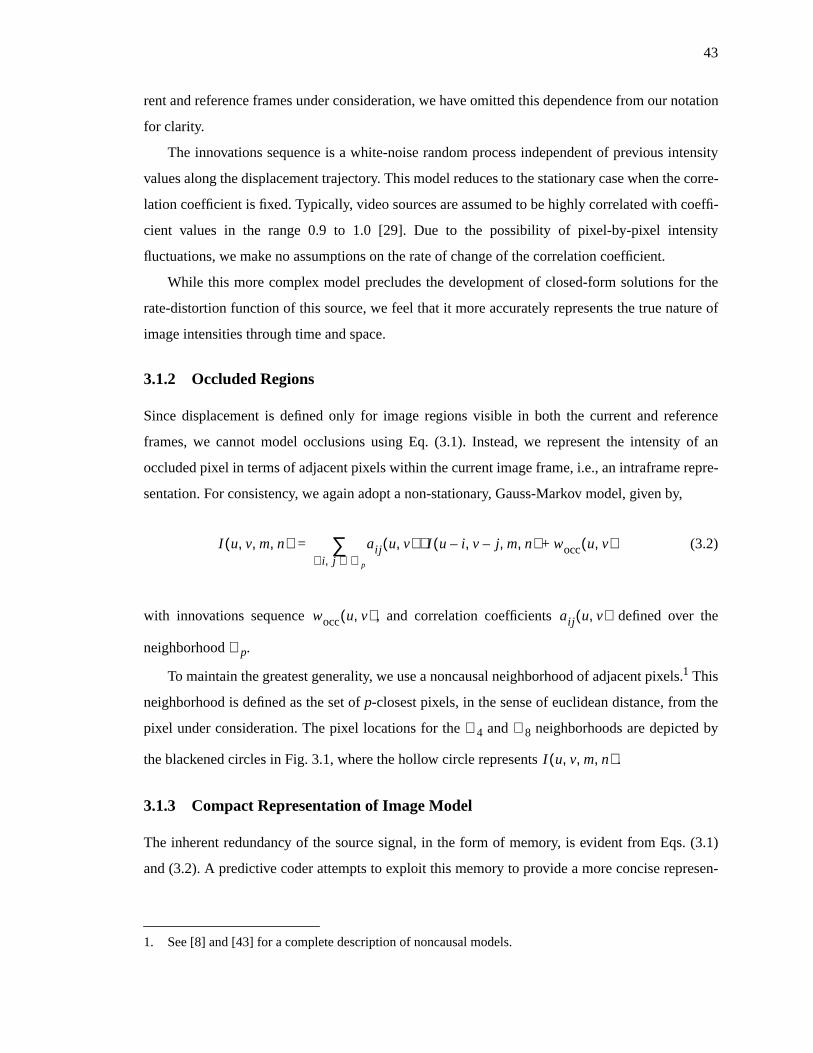
43
rent and reference frames under consideration, we have omitted this dependence from our notation
for clarity.
The innovations sequence is a white-noise random process independent of previous intensity
values along the displacement trajectory. This model reduces to the stationary case when the corre-
lation coefficient is fixed. Typically, video sources are assumed to be highly correlated with coeffi-
cient values in the range 0.9 to 1.0 [29]. Due to the possibility of pixel-by-pixel intensity
fluctuations, we make no assumptions on the rate of change of the correlation coefficient.
While this more complex model precludes the development of closed-form solutions for the
rate-distortion function of this source, we feel that it more accurately represents the true nature of
image intensities through time and space.
3.1.2 Occluded Regions
Since displacement is defined only for image regions visible in both the current and reference
frames, we cannot model occlusions using Eq. (3.1). Instead, we represent the intensity of an
occluded pixel in terms of adjacent pixels within the current image frame, i.e., an intraframe repre-
sentation. For consistency, we again adopt a non-stationary, Gauss-Markov model, given by,
(3.2)
with innovations sequence , and correlation coefficients defined over the
neighborhoodℵp.
To maintain the greatest generality, we use a noncausal neighborhood of adjacent pixels.1 This
neighborhood is defined as the set ofp-closest pixels, in the sense of euclidean distance, from the
pixel under consideration. The pixel locations for theℵ4 andℵ8 neighborhoods are depicted by
the blackened circles in Fig. 3.1, where the hollow circle represents .
3.1.3 Compact Representation of Image Model
The inherent redundancy of the source signal, in the form of memory, is evident from Eqs. (3.1)
and (3.2). A predictive coder attempts to exploit this memory to provide a more concise represen-
1. See [8] and [43] for a complete description of noncausal models.
I u v m n, , ,( ) aij u v,( ) I u i– v j– m n, , ,( )⋅i j ℵp∈,∀∑ wocc u v,( )+=
wocc u v,( ) aij u v,( )
I u v m n, , ,( )

44
tation of the multi-view signal. We next consider the task of generating a compact representation
for unoccluded regions.
The best linear mean square prediction of an unoccluded pixel, from a given reference frame,
is provided by the combination of correlation coefficient and displacement vector. If these parame-
ters are specified exactly, the error, or residual, between the actual and predicted pixel intensities
will equal the innovations sequence. Typically, the entropy of the residual image is considerably
less than that of the original image; hence, it can be encoded using fewer bits for a given level of
distortion. However, an excessive number of bits would be required to transmit the correlation
coefficient and displacement vector for each pixel. Since these quantities represent an over-deter-
mined set of parameters for the representation of the desired pixel, approximations of the image
model are often made to reduce the bit rate required to describe the prediction process.
Even though we hypothesize that our non-stationary model more accurately represents the true
progression of image intensities through a video signal, parameter estimation of the correlation
coefficient is a difficult process. This difficulty is due not only to the spatiotemporal variation of
the coefficient, but also to the fact that the actual displacement vectors are unknown and must be
estimated themselves. Therefore, one cannot directly calculate the covariance of the image intensi-
ties along displacement trajectories, which is required to estimate the best linear mean square pre-
diction filter. A common approximation then is through the use of a spatially-invariant prediction
filter, i.e., the filter is fixed over an entire image. Since the correlation coefficient of the image
model is sufficiently close to one, a unity filter tap is often employed. Although this prediction fil-
Figure 3.1:ℵ4 (a) andℵ8 (b) two-dimensional, noncausal neighborhoods.
u
v
u
v
a. b.
45
ter has a pole on the unit-circle, stability is not an issue since the output is bounded by the quanti-
zation of intensity values.
Another often used approximation is that contiguous regions of pixels have constant displace-
ment. This approximation is based on a rigid-body, translation displacement model. Only a single
displacement vector must be transmitted for each group of pixels, greatly reducing the bit rate of
the prediction.
Combining these approximations, the prediction of the pixel in the current frame, from the
corresponding point in the given reference frame is given by,
(3.3)
where and are interpreted as the average horizontal and vertical displacement components
of the image region assumed to possess constant displacement. This prediction is sub-optimal in
the sense that the error between the actual and predicted intensities no longer equals the innova-
tions sequence. Instead, the residual is correlated with the prediction, and generally requires more
bits to encode than that required for . Therefore, a trade-off exists between allocating
more bits to accurately represent the parameters of the image model or more bits to encode the
residual image. We discuss the ramifications of the predicted-residual image correlation and a
technique to exploit this information in Chapter 5.
A similar process is performed for the compression of occluded regions, where a single set of
correlation coefficients typically are assumed or estimated for the entire image frame. We note a
few observations on techniques used to obtain a compact representation for occluded regions.
The noncausal model lends itself to transform-based techniques [43]. This is the approach
taken by the MPEG class of video compression standards [2], where intraframe DCT-based com-
pression is performed on “poorly predicted” (read occluded) blocks within a predictively-coded
frame. The use of a fixed transform implies the assumption of a stationary image model. This con-
cept was extended in [24] to include image dependent statistics; an image block is coded using a
transform selected from a codebook of transforms designed off-line, each of which approximates
the KLT for a specific class of image sources. This approach can accommodate a finite number of
correlation variations.
Noncausal prediction, as described in [6], also can be used for the intraframe coding of occlu-
sions. Here, horizontal and vertical sample correlations are calculated over the entire image, and
I u v m n, , ,( ) I u du u v,( )– v dv u v,( )– mref nref,, ,( )=
du dv
wun u v,( )

46
are transmitted to the decoder. The image then is “whitened” using a backward representation of
the potential matrix, and the residual is encoded via a vector quantizer. The complexity of this
technique can be reduced, from its original form, since occlusions typically occupy only a rela-
tively small percentage of the image frame, and boundary values are readily available from neigh-
boring unoccluded regions.
Regardless of the method taken to generate a compact representation of occluded regions, in
general, substantially more bits are required to encode these regions as compared to unoccluded
regions; i.e., the entropy of is greater than that of . This discrepancy in rate-
distortion performance typically is most severe for highly-textured image regions, since the
intraframe model for these regions yields a poor prediction of the desired pixel intensity, in terms
of a large dynamic range for the prediction error.
Therefore, we wish to use the reference frame that has minimum occlusion with the current
frame for the frame-based prediction step of a multi-view hybrid encoder. We provide our solution
to the selection of the minimum-occlusion reference frame in Chapter 4.
3.2 Displacement Model
Displacement is formally defined as the vector difference between the pixel locations of corre-
sponding points in appropriately aligned image frames. Displacement is a function of scene struc-
ture, differential viewpoint parameters, object motion and temporal sampling rate.
The displacement vector for an unoccluded pixel in FrameA, with respect to reference Frame
B, is denoted by,
(3.4)
If there is no ambiguity, we will often omit the subscripts from our displacement notation. Since
displacement is undefined for occluded pixels, we set for these regions. We define the
displacement vector field (DVF) as the collection of displacement vectors over the entire image
frame:
, and (3.5)
wocc u v,( ) wun u v,( )
dA B← u v,( )duA B←
u v,( )
dvA B←u v,( )
=
d u v,( ) ∅≡
DVF d u v,( )= u 0 … U 1–, ,{ }∈∀ v 0 … V 1–, ,{ }∈∀

47
A useful quantity is the displacement vector discontinuity, which is defined as the difference
between displacement components of unoccluded pixels along the two image coordinates:
(3.6)
where and . These difference equations can be viewed as the partial
derivatives of the displacement along theu- andv-coordinates. We also use the form of Eq. (3.6)
for the discontinuity between adjacent image regions, when pixels within each region have con-
stant displacement.
When dealing with estimated displacement vectors, we will include a circumflex into this
notation, i.e., and respectively denote the estimated displacement and estimated
displacement discontinuity. Displacement estimates that are assumed to be inaccurate, based on
some knowledge of the reliability of the estimate, are likewise denoted by .
The complete estimated displacement vector field uniquely describes the frame-based predic-
tion of the current frame from Eq. (3.3). Fractional displacement estimates are handled in Eq. (3.3)
by performing some form of spatial interpolation to generate the intensity value at sub-pixel loca-
tions in the reference frame.
For simplicity, we assume a rigid-body, translational displacement model throughout this the-
sis, i.e., a contiguous region of pixels has constant displacement. Or, in terms of the scene, we
assume that the scene consists of a collection of “small” planar surfaces, which are perpendicular
to the camera axis and exhibit only planar motion between the temporal samples of the current and
reference frames. This model represents the relatively complex, affine geometric transformations
of rotation and scaling as a set of piecewise linear translations.
The displacement component along its corresponding image coordinate is a staircase function;
i.e., it consists of a set of flat regions with distinct jumps at the boundaries between objects either
located at different depth planes (for spatially-offset frames), or possessing differential velocities
(for temporally-offset frames). The displacement discontinuity then is a series of Kronecker delta
functions located at object boundaries.2
2. In statistical terms, the displacement along an image row (column) can be modeled as a generalizedPoisson process, and the displacement discontinuity as a generalized Poisson impulse process [73],where the location of the Poisson points are correlated between adjacent image rows (columns).
∆d u v,( )∆du u v,( )
∆dv u v,( )
du u v,( ) du u 1– v,( )–
dv u v,( ) dv u v 1–,( )–= =
du 1– v,( ) 0≡ dv u 1–,( ) 0≡
d u v,( ) ∆d u v,( )
d u v,( ) ∅=

48
We next develop two fundamental principles based on the rigid-body, translation displacement
model. We follow this by describing a reliability measure for block-based displacement estimates.
These results will be used extensively in Chapters 4 and 6 for the processing of noisy displacement
vector fields.
3.2.1 One-to-One Mapping of Unoccluded Regions
Consider an image region,ℜA, in FrameA that is visible in reference FrameB at the corresponding
region denoted byℜB. We describe this relationship by stating that, “ℜB maps toℜA”. Obviously,
the reverse relationship holds:ℜB is visible in FrameA atℜA. This bidirectional relationship rep-
resents the one-to-one mapping between unoccluded regions.
Neglecting image noise and lighting variations from Eq. (3.1), the intensity of an unoccluded
pixel in FrameA is expressed in terms of the intensity of the corresponding point in FrameB from
Eq. (3.7a), and the mapping of corresponding pixels from FrameA to FrameB is given by Eq
(3.7b).
(3.7a)
(3.7b)
We define the change of variables, and . Substituting
these quantities and reversing the left-hand and right-hand sides of Eq. (3.7a) yields,
(3.8)
Equating Eq. (3.8) with Eq. (3.7b), we obtain the relationship between bidirectional displacement
vectors for unoccluded regions:
(3.9)
This result implies that the displacement vector field relating FrameB from FrameA is uniquely
specified from the DVF of FrameA from FrameB. Therefore, given a unidirectional displacement
field, the complete reversed field is obtained by calculating the displacement vector for each pixel
I u v A, ,( ) I u duA B←u v,( )– v dvA B←
u v,( )– B, ,( )=
I u v B, ,( ) I u duB A←u v,( )– v dvB A←
u v,( )– A, ,( )=
u' u duA B←u v,( )–= v' v dvA B←
u v,( )–=
I u' v' B, ,( ) I u' duA B←u v,( )+ v' dvA B←
u v,( )+ A, ,( )=
dB A← u duA B←u v,( )– v dvA B←
u v,( )–,( ) d– A B← u v,( )=

49
using Eq. (3.9). We may also use this relationship to disregard displacement estimates that are
inconsistent with the one-to-one mapping. A final observation is that the number of occluded pix-
els in FrameA, with respect to FrameB, equals the number of occluded pixels in FrameB, with
respect to FrameA.
3.2.2 Occlusion / Displacement Discontinuity Relationship
We establish the fundamental property relating occlusion and displacement discontinuity by exam-
ining the source of occluded regions.
Assume that a real-world object lies completely within a camera’s field-of-view and is located
between the camera and some scene background. An occlusion is caused by the foreground object
if and only if the camera viewpoint changes or the object moves with respect to the background
between frames. For either case, the displacement of the foreground object differs from that of the
scene background, i.e., a displacement discontinuity exists.
We demonstrate the occlusion / displacement relationship by examining the effect of a dis-
placement discontinuity in a unidirectional field on the reversed field. Let the horizontal displace-
ment components of two adjacent unoccluded pixels within DVFA←B equal d1 and d2,
respectively:
and (3.10)
To simplify the notation, we assume that . Substituting these
quantities into Eq. (3.9) yields the horizontal displacements for the two corresponding points in the
reversed field:
(3.11a)
(3.11b)
If , then . However, if a discontinuity exists at this location, the two adjacent
pixels in FrameA are mapped from non-adjacent pixels in FrameB. While the region between
in FrameB might map to another region in Frame A, it is more likely that this region is
occluded, where the horizontal length of the occlusion equals .
duA B←u 1– v,( ) d1= duA B←
u v,( ) d2=
dvA B←u 1– v,( ) dvA B←
u v,( ) 0= =
duB A←u 1– d1– v,( ) d1– duB A←
u1 v,( )= =
duB A←u d2– v,( ) d2– duB A←
u2 v,( )= =
d1 d2= u1 u2 1–=
u1 u2,( )
d1 d2–
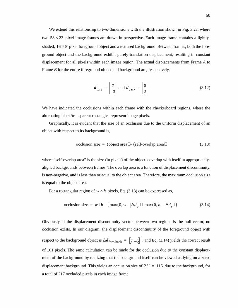
50
We extend this relationship to two-dimensions with the illustration shown in Fig. 3.2a, where
two pixel image frames are drawn in perspective. Each image frame contains a lightly-
shaded, pixel foreground object and a textured background. Between frames, both the fore-
ground object and the background exhibit purely translation displacement, resulting in constant
displacement for all pixels within each image region. The actual displacements from FrameA to
FrameB for the entire foreground object and background are, respectively,
and (3.12)
We have indicated the occlusions within each frame with the checkerboard regions, where the
alternating black/transparent rectangles represent image pixels.
Graphically, it is evident that the size of an occlusion due to the uniform displacement of an
object with respect to its background is,
(3.13)
where “self-overlap area” is the size (in pixels) of the object’s overlap with itself in appropriately-
aligned backgrounds between frames. The overlap area is a function of displacement discontinuity,
is non-negative, and is less than or equal to the object area. Therefore, the maximum occlusion size
is equal to the object area.
For a rectangular region of pixels, Eq. (3.13) can be expressed as,
(3.14)
Obviously, if the displacement discontinuity vector between two regions is the null-vector, no
occlusion exists. In our diagram, the displacement discontinuity of the foreground object with
respect to the background object is , and Eq. (3.14) yields the correct result
of 101 pixels. The same calculation can be made for the occlusion due to the constant displace-
ment of the background by realizing that the background itself can be viewed as lying on a zero-
displacement background. This yields an occlusion size of due to the background, for
a total of 217 occluded pixels in each image frame.
58 23×
16 8×
dfore7
3–= dback
0
2=
occlusion size object area( ) self-overlap area( )–=
w h×
occlusion size w h max 0 w ∆du–,( ) max 0 h ∆dv–,( )⋅{ }–⋅=
∆dfore-back 7 5–t
=
2U 116=

51
u
v
u
v
(-7,3)
(7,-3)
Figure 3.2: Relationship between occlusion and unoccluded region displacementdiscontinuity, a) sample frames with constant displacement for background andforeground object, b) vertical component of actual displacement along middle imagecolumn.
(0,2)
(0,-2)
a.
FrameA
FrameB
v
FrameB
FrameA
b.

52
The actual vertical displacement component of the middle image column is shown in Fig.
3.2b. Pixels are indicated by the shaded rectangles along each image column, where occlusions are
denoted by the blackened pixels. The slanted-lines connecting unoccluded pixels represent
. We observe that occlusions occur in FrameB only at the location of displacement dis-
continuities in FrameA, and vice versa. In particular, for this image column, the number of
occluded pixels is equal to the absolute value of the sum of all negative∆dv’s.
The calculation of the exact amount of occlusion becomes more difficult than the simple
expression of Eq. (3.14) when dealing with more complexly-shaped objects and situations of mul-
tiple, mutually-occluded objects; however, the fundamental relationship between occlusion and
displacement discontinuity still holds. Using this property, the location and size of occlusions
within the reference frame can be calculated from the discontinuites in the displacement vector
field of the current frame.
3.2.3 Reliability of Block-based Estimates
Since we have assumed rigid-body, translational displacement, only a single displacement vector
is required to describe the displacement of a contiguous region of pixels. Hence, a block-based
technique can be used to estimate these displacement vectors. In these techniques, the current
frame is partitioned into a set of non-overlapping blocks, where the blocks may be either fixed- or
variable-sized.3 A search is performed for each block in the current frame for the block in the ref-
erence frame that yields the minimum distortion. The estimated displacement vector is merely the
vector difference between the location of the original block and the minimum-distortion reference
block. Common causes of displacement estimation errors are when: the block has relatively uni-
form intensity, a displacement discontinuity occurs within a block, or the block contains occluded
pixels.
A simple measure of the reliability of an estimate is provided by the prediction signal-to-noise
ratio of the respective block, where the noise is defined as the distortion between the original block
and the corresponding block in the reference frame. The SNR is a more accurate reliability mea-
sure than merely the distortion, due to the problems encountered when the original block has rela-
tively low intensity variation. For these regions, the prediction distortion for all possible
3. The optimal block-dimensions for fixed-sized block-based techniques can be related to the relativecost incurred when coding a block with one or more displacement discontinuities and the densityparameter of the generalized Poisson process that models the displacement along each image coor-dinate (see footnote 2).
dv 29 v,( )

53
displacements within a uniform region in the reference frame will be approximately zero. It is
unlikely that the actual displacement for this block will be estimated correctly since multiple refer-
ence blocks yield nearly identical distortion. However, the prediction SNR for this block will be
low, indicating a high probability of error.
Therefore, the prediction SNR can be used as a rough detection criteria for erroneous esti-
mates. It can also be used to rank displacement estimates, based on the probability of error, when a
single displacement vector must be selected from two or more possible estimates.

54
Chapter 4
Optimal Reference Frame Selection
In this chapter, we examine the problem of selecting the optimum reference frame1 for the predic-
tive coding of multi-view video signals. We begin with a brief review of the effect of occlusions on
prediction performance, and demonstrate the need for adaptive reference frame selection. We then
present our novel selection algorithm that estimates the prediction performance that would be
obtained from using a particular reference frame without requiring the computationally costly pro-
cess of displacement estimation for each candidate reference. This approach relies on the relation-
ship between occlusion and displacement discontinuity of unoccluded regions (Section 3.2.2) to
select the reference frame that yields the best rate-distortion prediction performance.
The main contributions of this work are: 1) a set of simple tools to eliminate likely false esti-
mates from a noisy displacement vector field, 2) the indirect estimation of a candidate reference
frame’s displacement field through the combination of multiple,single-step DVF’s into acompos-
ite field, and 3) a variance-based measure to estimate the amount of occlusion between two frames
from a composite displacement field. This technique achieves impressive prediction and compres-
sion performance, while requiring an inconsequential number of bits to specify the selected refer-
ence frame and acceptable complexity and storage costs. We illustrate the superiority of this
algorithm through comparisons with both non-adaptive and exhaustive search approaches.
4.1 Prediction Performance
Frame-based predictive coders attempt to minimize both the distortion between the predicted and
original frames and the number of bits needed to describe the prediction. The rate-distortion per-
formance of the prediction process is related to numerous factors, including the frame sampling
1. The reference frame is said to be optimum when the rate-distortion prediction cost is minimized.

55
frequency, scene and camera motion, and the sophistication of the predictor’s motion model. Prob-
ably the most basic factor affecting performance is the amount of occlusion between the reference
and desired frames. Since frame-based predictors typically do not distinguish between occluded
and unoccluded regions, only regions within the desired frame that are present in the reference
frame can be predicted accurately. Conversely, the prediction process will fail for regions within
the desired frame that are occluded from the reference frame. Two frames are void of occlusion
when the scene objects are static with respect to the viewpoints of each frame; perfect prediction is
possible for this situation. The other extreme occurs when two frames have no corresponding
points.
Equivalently, prediction performance is related to thesimilarity of the desired and reference
frames, which we quantify as the complement of occlusion. Here, our definition of occlusion
incorporates all image regions that prove difficult for the particular prediction process used,
regardless of the source of this difficulty. Therefore, it is possible for a region to be “visible” to an
observer, yet be classified as occluded. For example, since we assume a translational displacement
model, if a region undergoes deformation (e.g., morphing) between two frames, an accurate pre-
diction of this region will not be possible and we characterize it as being occluded.
To achieve superior prediction and, hence, compression performance, the reference frame that
has minimum occlusion (maximum similarity) with the desired frame should be used in the predic-
tion process. For the case of single-view video signals, the relative amount of occlusion between
frames is obvious; in the absence of any inherent camera or scene object motion periodicity, the
temporally closest frames generally can be assumed to have the least amount of occlusion with the
desired frame. Indeed, this relationship is utilized in the MPEG and H.26x classes of video com-
pression standards, where the temporally closest previous and/or future decoded reference frames
are used for the prediction ofP-, B-, andPB-frame types.
The similarity relationship between frames in a multi-view video signal is not as straightfor-
ward. We next describe three scenarios that illustrate the need for adaptive reference frame selec-
tion to ensure that the most similar reference frame is used in the prediction process.
4.2 Multi-view Scenarios
For the first scenario, we consider a video signal consisting of two views with relatively large dif-
ferential viewpoint parameters, resulting in a high degree of inter-view occlusion. Assuming that
the camera and scene object motion is slow with respect to the frame rate, temporally adjacent
frames within each view will be quite similar. For this situation, the optimum reference frame

56
would be the frame previous in time and within the same view (i.e., the temporally-offset, intra-
view reference frame).
In the second scenario, the multi-view signal is comprised of three views with synchronized
temporal sampling and arbitrary viewpoints, where the relative viewpoint parameters are such that
a high degree of scene-overlap exists among the views. If the camera and/or scene object motion is
rapid or complex, with respect to the predictor’s displacement model, the temporally-offset, intra-
view frame will have a large amount of occlusion with the desired frame. Instead, a superior pre-
diction will be obtained by using a reference frame from one of the other views, whose temporal
index matches that of the desired frame (i.e., a temporally-equivalent, inter-view reference frame).
The selection between which of the two possible views to use for the reference frame depends on
the camera configuration and the direction of the motion.
Our final scenario demonstrates the possibility of the relative location of the best reference
frame being offset from the desired frame in both time and viewpoint. Let the multi-view signal
consist of two views, whose relative camera viewpoints are fixed. If the scene is slowly-varying
and the absolute viewpoint parameters exhibit motion in the direction of the differential values, a
temporally-offset, inter-view frame may yield the best prediction.
Such a scenario is illustrated in Fig. 4.1, where the scene is static, the viewpoints are separated
by a horizontal distance of∆cx for the duration of the sequence, and the camera motion is purely
horizontal. The curved, dotted-line traces the motion of the cameras through time, and the thumb-
nail images depict the spatiotemporal frame locations within each view. Since the scene objects are
motionless, the amount of occlusion is related directly to the spatial distance between frames.
Consider the prediction and compression of frames in View 0. Frame is spatially-
closest to and should be used for the prediction of this frame. For the next two temporal
samples, the most similar reference frames are the previous frames in time; i.e., predict
from . From till , the camera velocity is constant, and is equal to .
The perfect camera position alignment for this scenario yields:
, and (4.1)
Each of these frames can be reconstructed exactly from knowledge of the appropriate temporal
offsets and the corresponding frames in View 1; thus, they can be compressed extremely com-
pactly. The camera motion slows for the final two temporal samples. is equidistant from
F 1 0,( )
F 0 0,( )
F 0 n,( )
F 0 n 1–,( ) t 3T= t 5T=∆cx
T---------
F 0 3,( ) F 1 0,( )= F 0 4,( ) F 1 3,( )= F 0 5,( ) F 1 4,( )=
F 0 6,( )

57
cx
t
T
2T
6T
5T
4T
3T
7T
0
∆cx
View 0 View 1
Figure 4.1: Two-view scenario illustrating time-varying location of the optimalreference frame.

58
both and – optimum prediction performance would be obtained from using either
frame as the reference (or possibly both). The remaining frame should use the previous, intra-view
frame. Table 4.1 summarizes the best reference frames for this simulated signal.
From these scenarios, it is evident that the relative location of the optimum reference frame is
time-varying and signal-dependent. However, in all prior work known to the author on the predic-
tive coding of multi-view signals, the reference frames have been fixed and heuristically chosen [5,
7, 15, 78, 86, 87]. While the reasoning behind pre-selecting the reference frame has not been
explicitly mentioned in the literature, we feel that this approach is due to the naive replication of
single-view techniques or the overreliance on the epipolar-line-constraint.
4.3 Early Thoughts on Selection Algorithms
We next describe two approaches for the adaptive selection of the best possible reference frame for
the predictive coding of multi-view video signals. The first approach is a brute-force solution that
performs an exhaustive search on all candidate reference frames. The second approach utilizes the
established relationship between occlusion and prediction performance to perform the selection,
and is the foundation of our solution. The relative performance and costs of these techniques are
provided in Sections 4.5 and 4.6.
4.3.1 Exhaustive Prediction
Theoretically, the simplest reference frame selection technique would be to predict the desired
frame from all possible reference frames and then use the frame that yielded the best prediction.
While this method is guaranteed to achieve optimum prediction performance, its implementation
is impractical. In many video coders, the prediction operation consumes the largest share of the
processing cycles available. The number of prediction operations required at each temporal index
for an exhaustive search is quadratic in the number of views.
F 0 5,( ) F 1 5,( )
Original F(0,0) F(0,1) F(0,2) F(0,3) F(0,4) F(0,5) F(0,6) F(0,7)
Reference F(1,0) F(0,0) F(0,1) F(1,0) F(1,3) F(1,4) F(1,5) F(0,6)
Table 4.1: Optimal reference frames for View 0 in simulated multi-view signaldepicted in Fig. 4.1.

59
The complexity of this approach can be reduced through the use of a subband decomposition
of the image frames. Here, the image data is consecutively low-pass filtered and sub-sampled by a
factor of two in both image directions, resulting in a pyramidal image frame structure and dimin-
ished prediction complexity. Depending on the number of pyramid levels, performing the predic-
tion operation on each possible reference frame might be practical. However, due to the loss of
higher-frequency image components, the prediction performance for the low-resolution image
subband may not be consistent with the performance for the entire frame, and the selection of the
optimum reference frame can no longer be guaranteed.
4.3.2 Occlusion-based Selection
An alternative approach for the selection of the optimum reference frame would be to use an esti-
mate of the amount of occlusion as the selection criteria. Previously reported techniques for the
detection of occluded regions typically use a measure of symmetry between estimated, bidirec-
tional displacement vectors fields as the decision threshold [13, 83]. The problem with using these
occlusion estimation techniques for our reference frame selection task is that the estimation of a
displacement vector field is equivalent to performing a frame-based prediction; i.e., we have
merely reformulated the exhaustive search method.
We thus redefine the problem of selecting the best reference frame as: develop an estimate of
the relative amount of occlusion that avoids performing frame-based prediction for each candidate
reference frame. We can simplify this problem by realizing that we only are concerned with the
relative amount of occlusion, not the actual location of the occluded regions. Occlusion localiza-
tion is the goal of conventional occlusion detection schemes, and also the major source of diffi-
culty, due to the circular nature of this problem. We describe our occlusion estimation algorithm
that satisfies this complexity constraint in the following section.
4.4 New Algorithm
We calculate the relative amount of occlusion between frames from the degree of discontinuity in
the estimated displacement vector field for unoccluded regions, where the requisite vector fields
for each candidate reference frame are estimated indirectly.
We first perform a frame-based prediction of the desired frame from only one reference frame.
The reference frame for thissingle-step predictionis specified to ensure that any possible refer-
ence frame can be reached by stepping along multiple predictions. Since we only want to calculate

60
the degree of discontinuity from reliable, unoccluded region displacement vectors, we make use of
broad assumptions to eliminate probable estimation errors. We disregard the single-step displace-
ment estimate of a region if its prediction signal-to-noise ratio falls below a given threshold. We
also eliminate displacement estimation errors through the process of vector field reversal, which
utilizes the one-to-one relationship of the actual displacement of corresponding points between
two images. We complete the unoccluded region detection by discarding displacement estimates
along the image border based on the mean displacement vector.
A composite displacement vector field for each candidate reference frame then is obtained
through simple vector addition of processed single-step fields. For simplicity, we use a slightly
modified calculation of the variance of the composite displacement vector field as the measure of
discontinuity. The frame with minimum composite vector field variance is assumed to have the
least amount of occlusion with the desired frame and is selected as the best reference frame. This
approach also can be used to select multiple reference frames – the desired frame is predicted once
from each reference frame in the set ofNref frames with the lowest composite field variance; a final
prediction then is obtained by combining these predictions.
If the desired frame is to be predicted from only one reference frame, this algorithm requires a
maximum of two frame-based predictions: if the minimum variance frame was used in the single-
step prediction process, the predicted image is generated from the previously estimated, unproc-
essed displacement vector field; otherwise, an additional prediction is performed using the selected
frame. The major cost of this technique is the large amount of storage needed for the possible ref-
erence frames and the retention of the single-step displacement vector fields.
It should be noted that this algorithm can use sub-sampled image data to perform the reference
frame selection, as described in Section 4.3.1. Again, a trade-off exists between using higher-reso-
lution image subbands to improve the accuracy of the selection and using lower-resolution data to
reduce the complexity. However, since the complexity of the individual steps of eliminating likely
estimation errors, generating the composite fields and calculating the displacement variance are on
the order of one operation-per-pixel, our approach should be substantially less complex than the
sub-band exhaustive search technique.
A flow-chart depicting our reference frame selection algorithm is shown in Fig. 4.2. The vari-
ous steps of our algorithm are described in detail in the following sub-sections.

61
Figure 4.2: Flow-chart for adaptive reference frame selection algorithm.
EstimateOcclusion withinComposite Field
All ReferenceFrames Checked?
NO
YES
Predict Frame fromMinimum OcclusionReference Frame(s)
PerformSingle-stepPrediction
DetectUnoccluded
Regions
Generate CompositeField for PossibleReference Frame

62
4.4.1 Composite Displacement Vector Fields
The composite fields for each candidate reference frame are obtained through the vector addition
of multiple, processed, single-step displacement vector fields. The single-step fields provide the
displacement relationship between two frames in the multi-view signal, and are the basic building
block for the generation of the composite fields. Prior to vector addition, the single-step fields are
processed to eliminate false estimates that would otherwise corrupt the occlusion measure.
4.4.1.1 Single-step Predictions
The first task in the generation of the composite displacement vector fields is the specification of a
set of single-step predictions. These predictions must be ordered to ensure that each possible refer-
ence frame can be “reached” through the combination of successive single-step displacement vec-
tor fields.
We assign one of the views in the multi-view signal as theindependent view. This view is
coded using any combination of user-specifiedI-, P- andB-frame types, where the predictively-
coded frames use only intra-view reference frames. This stipulation of an independently coded
view does not result in an overall loss of compression performance since prediction cannot be per-
formed circularly, e.g., it is impossible to predict both from and
from . The forward predictions are used as the single-step predictions for the indepen-
dent view, and the associated displacement vector fields are retained.
A reference view then is assigned for each of the remaining,dependent views in the signal.
The assignment of the reference views must satisfy the following constraints: 1) at least one
dependent view must use the independent view as its reference, and 2) the independent view must
be accessible to all other dependent views through successive dependent/reference view links.
These constraints ensure a prediction relationship between all views and also avoid any circular
predictions. The single-step displacement vector field for each frame in a dependent view is
obtained by predicting the desired frame from the frame in its reference view with the same tem-
poral index. All frames within the dependent views will eventually be predicted using an adap-
tively selected reference frame.
We illustrate the single-step predictions for a three-view signal in Fig. 4.3a, where the bold,
vertical bars represent frames within each view. Both Views 1 and 2 reference the independent 0th
view, whose frame-type structure, for the five frames shown, isIBPBP. The curved arrows denote
the single-step predictions of a desired frame (arrow head) from a reference frame (arrow tail).
F m1 n1,( ) F m2 n2,( ) F m2 n2,( )
F m1 n1,( )

63
View 0
View 1
View 2
t
View 0
View 1
View 2
Figure 4.3: Three-view reference frame location scenario, a) single-step predictions,b) possible reference frames for a maximum temporal-offset of two frames.
a.
b.
0 T 2T 3T 4T
t0 T 2T 3T 4T

64
Only the forward prediction of the bidirectionally-predicted (B) frame is used as a single-step pre-
diction. We observe that any frame within this structure can be reached from any other frame by
stepping along successive prediction links. The dependent view predictions are used to step
between views, and the independent view’s single-step predictions allow for stepping in time.2 We
discuss the actual method of stepping along the single-step predictions to generate the composite
displacement vector fields in Section 4.4.1.3.
Since we assume that the minimum-occlusion reference frames will be temporally close to the
desired frame, we assign a maximum temporal-index delay, , which specifies the relative
temporal range of the possible reference frames. The complete set of reference frames is given by
this delay and the independent view’s frame type structure. To illustrate the relative reference
frame locations, we order the views such that is the independent view, is a depen-
dent view that references the independent view, references either or the indepen-
dent view, and so on. This ordering was used in Fig. 4.3a. Assuming that only P or B frames are
used in the independent view for frames within , a frame in a dependent view,
, then may be predicted from: 1) any independent view frame within , 2)
the frame previous in time and within the same view, or 3) any other dependent view frame within
the negative half of the temporal range, less the same temporal index if the reference view number
is greater than that of the desired frame’s. The relative locations of the possible reference frames,
, are summarized by,
(4.2)
Figure 4.3b depicts the possible references frames for the prediction of a desired frame in our
three-view signal, where and the dashed vertical bars represent uncoded frames.
2. If an I-frame type is present in the independent view, frames that have temporal indices equal to orbeyond this frame (in the sense of the temporal direction of the stepping) cannot be reached.
∆nmax
F 0 n,( ) F 1 n,( )
F 2 n,( ) F 1 n,( )
n ∆nmax±
F m 0≠ n,( ) n ∆nmax±
F mref nref,( )
nref
n ∆nref– … n ∆nref+, ,{ } , if mref 0=
n ∆nref– … n 1–, ,{ } , if mref m<
n 1–{ } , if mref m=
n ∆nref– … n, ,{ } , if mref m>
∈
∆nmax 2=

65
Here, a total of eight composite displacement vector fields must be generated and analyzed for the
prediction of . For the general case, the total number of possible reference frames for each
desired frame, in themth view, is:
(4.3)
4.4.1.2 Unoccluded Region Detection
Since we only want to use the actual displacement vectors for unoccluded regions in our occlusion
measure, we wish to exclude any single-step displacement vector estimates that have a high proba-
bility of error. Erroneous estimates may occur due to limitations of the prediction process or the
meaningless calculation of displacement for occluded regions.
We use the prediction block-SNR as a confidence measure of the accuracy of each displace-
ment estimate, as described in Section 3.2.3. The single-step displacement vector estimate associ-
ated with a region whose prediction PSNR falls below a user-defined threshold is assumed to be
erroneous, and is discarded from any further consideration.
The thresholding process can be viewed in terms of a classical, binary detection problem [96].
We observe the prediction PSNR for a particular displacement estimate, where the statistics of the
PSNR are governed by whether the estimate is either correct or incorrect. The threshold then is
based on some knowledge of these statistics and the relative costs of false alarms (i.e, say estimate
correct when it is not) and misses. For this application, we are most concerned with obtaining a
low probability of false alarm, so we generally will use a conservative (i.e., relatively high) thresh-
old.
We illustrate the displacement vector thresholding in Fig. 4.4 for a one-dimensional case. Fig-
ure 4.4a depicts the displacement predicting pixels in FrameB from FrameA, where a single dis-
placement value was estimated for each set of five neighboring pixels. The prediction signal-to-
noise ratios for each 5-pixel region are labelled such that . Only is less
than the given threshold and the associated displacement estimates are eliminated in Fig. 4.4b.
Here, the blackened pixels do not necessarily represent occlusions, but merely that the displace-
ment estimate for this region was likely inaccurate.
F 1 2,( )
ηref m( ) M ∆nmax m 1+ +⋅=
SNRi SNRi 1+> SNR5

66
Once thresholded, we can further eliminate false estimates by using the one-to-one relation-
ship between the true displacement of corresponding points from FrameA to FrameB, and vice
versa, satisfies:3
(4.4)
If the estimated displacement vector field is inconsistent with this relationship, we assume that an
error has occurred and eliminate the likely false estimate.
3. See Eq. (3.9) in Section 3.2.1.
dA B← u duB A←u v,( )– v dvB A←
u v,( )–,( ) d– B A← u v,( )=
Figure 4.4: Displacement vector thresholding and field reversal, a) original field, b)field after SNR thresholding, c) reversed field.
FrameA
FrameB
FrameA
FrameB
FrameA
FrameB
SNR3 SNR2 SNR1 SNR5 SNR4
a.
b.
c.
SNR3 SNR2 SNR1 SNR4
67
Given a single-step displacement vector field in one direction, we examine the usage of the
pixels in the reference frame. If a reference pixel is used for the prediction of only one pixel in the
desired frame, we assume that this displacement estimate is accurate and assign the reversed dis-
placement vector according to Eq. (4.4). Conversely, if a pixel is referenced by more than one dis-
placement vector, we are assured that all of these estimates cannot be correct. Again, we use the
prediction SNR for the decision as to which of these estimates has the lowest probability of error.
The displacement estimate for the reference pixel is assigned the negative of the forward displace-
ment vector with maximum prediction SNR, and all other vectors are invalidated. Finally, if a pixel
in the reference frame is not used in the prediction, we assume that this pixel is occluded and do
not assign a reversed displacement estimate to it. The field reversal process not only detects unoc-
cluded regions, but also provides valid displacement vector estimates in both directions that satisfy
Eq. (4.4), i.e., it generates from . This information will be used to step
along single-step predictions in both directions.
Figures 4.4b and 4.4c illustrate the process of eliminating displacement estimates that do not
satisfy the one-to-one mapping of actual unoccluded region displacements. The bidirectional
arrows in Fig. 4.4c indicate that these displacement values map corresponding pixels from Frame
A to FrameB, and vice versa. Again, the blackened pixels represent regions whose displacement
estimate has been invalidated. We note that even though the displacement was estimated for con-
tiguous regions of five pixels, only individual pixel displacement vectors are eliminated. Since the
displacement estimate might be accurate for portions of the region, we do not eliminate the dis-
placement for entire regions if a subset of its displacements is inconsistent with Eq. (4.4).
The final step in the detection of highly reliable displacement estimates is the elimination of
displacement vectors along the image borders. We assume that the global displacement of the
image background between image frames is given by the mean displacement vector of the single-
step field after thresholding and field reversal. If the mean vector is non-zero, pixels along the
appropriate horizontal and vertical image borders are likely occluded. The width and height of the
occluded region are, respectively, equal to the magnitude of the horizontal and vertical compo-
nents of the mean vector, and the appropriate border sides depend on the sign of the individual
components. For example, if the mean displacement vector is , we assume that a border
occlusion exists for the vertical strip of three pixels along the left image border and horizontal strip
of five pixels along the top border.
dA B← u v,( ) dB A← u v,( )
3– 5t

68
We first calculate the mean vector for all valid vectors in the single-step field and round the
vector to integer values. Here, we invalidate an entire image region of constant displacement if one
or more pixels within the region lies within the border occlusion. This differs from our approach to
the elimination of displacement estimates that were inconsistent with the one-to-one mapping of
actual displacement vectors. Since only a relatively limited number of image regions will lie
within the border occlusion, we can afford to be much more cautious as to which estimates to
retain.
4.4.1.3 Vector Field Addition
The composite displacement vector field for each possible reference frame is obtained through the
simple vector addition of the processed single-step fields. Given two displacement vectors fields
FrameA
FrameB
FrameA
FrameC
FrameC
FrameB
Figure 4.5: Generation of composite displacement vector field through field addition,a) and b) single-step displacement fields, c) composite field.
a.
b.
c.
69
predicting FrameA from FrameB ( ), and FrameB from FrameC ( ), the
composite field relating framesA andC is given by,
(4.5)
where the combined fields may be either single-step or composite fields. If FrameC is actually
FrameA, substituting Eq. (4.4) into (4.5) yields , as expected. The normal asso-
ciative and commutative properties also hold for the addition of vector fields.
The generation of composite fields relies on the property that a region unoccluded in FramesA
andB and also unoccluded in FramesB andC will be unoccluded between FramesA andC.4 The
displacement of unoccluded regions between the desired frame and its possible reference frames,
thus, can be estimated without the costly process of displacement estimation for each reference
frame. However, it should be noted that the composite displacement vector fields cannot be used
directly to provide an accurate estimate of prediction performance. The composite fields are gener-
ated for regions that are assumed to be unoccluded, and do not cover the entire image frame. The
resulting prediction performance from using these fields will likely be unrelated to the actual per-
formance for the complete frame.
In Fig. 4.5, we illustrate the addition of two displacement fields in one-dimension, where the
field relating FramesA andB is the processed single-step field from Fig. 4.4a. The majority of the
displacements of the resulting composite field between FramesA andC are close to zero, with
only one relatively large estimate in the middle of the field.
4.4.2 Occlusion Measure
For each composite field, we approximate the displacement discontinuity, and hence amount of
occlusion, from a modified variance calculation of valid displacement estimates. The modification
is the result of augmenting the composite field with a region of zero-displacement vectors. If used
in its initial, unaltered form, the variance of the composite DVF provides a measure of the relative
amount of inter-object occlusion. By augmenting the DVF, occlusions along the image borders,
due to the displacement of the background, are also accurately estimated.
4. The converse of this property obviously does not hold; nor will a region in FrameA that is occludedfrom FrameB necessarily be occluded from FrameC.
dA B← u v,( ) dB C← u v,( )
dA C← u v,( ) dA B← u v,( ) dB C← u duA B←u v,( )– v dvA B←
u v,( )–,( )+=
dA A← u v,( ) 0=

70
For example, consider a field where each valid displacement estimate equals the same non-
zero vector. The variances of the horizontal and vertical components of this field obviously will be
zero. However, occlusions are present on the image border, which may represent a substantial por-
tion of the entire frame.
We assume that the background has constant displacement equal to the mean displacement
vector of composite field. The mean values, and , are calculated from the valid displace-
ment estimates, and are substituted for the displacement discontinuity components in Eq. (3.14) to
yield the size of the augmented region:
(4.6)
where the functions from Eq. (3.14) have been removed since we are assured that
and . Finally, the relative occlusion measure between the desired and possible
reference frame is given by the sum of the variances of the displacement vector components of the
augmented field:5
(4.7)
This occlusion measure is a function of both the mean and variance of the composite displacement
vector field, and, thus, adequately approximates both inter-object and background displacement
discontinuity.
Returning to our example one-dimensional field in Fig. 4.5, we observe that the occlusion
measure for the field in Fig. 4.5c is significantly less than the top field, and FrameC would be
selected as the reference frame for the prediction of FrameA.
4.5 Cost Analysis
In this section, we compare the relative encoder complexity and storage costs of using the
described, adaptive algorithm versus an exhaustive search for the selection of the optimal refer-
ence frame; these costs are fixed for the multi-view decoder. Since the prediction and coding of the
5. We have experimented with a more sophisticated occlusion measure based on a direct applicationof Eq. (3.13), only to find the simple variance calculation more robust to spurious estimates.
µdu
µdv
augmented size U µdu
V µdv
µdu
µdv
⋅–⋅+⋅=
max( )
U µdu
≥ V µdv
≥
occlusion measure σdu
2 σdv
2+=

71
independent views are identical for both selection methods, the analysis is performed only on the
dependent views. A fixed, pre-selected reference frame scheme is used as the baseline for the com-
parison. We assume that the desired frame is predicted from reference frames (typically one
or two frames).6
4.5.1 Complexity
For a fixed reference frame scheme, the total complexity to generate the final predicted image is
given by,
(4.8)
where is the complexity of performing a frame-based prediction and is the
complexity of combining multiple predictions, with . If a full-search prediction
process is used, is on the order of the search area in pixels, where we have assumed, for sim-
plicity, that the search ranges for each reference frame are equal.
The prediction of the desired frame using an exhaustive search selection technique amounts to:
1) generating a prediction from each possible reference frame, 2) calculating the prediction distor-
tion for each reference, and 3) selecting and combining the minimum distortion predictions.
The average number of possible reference frames, for each desired frame, is obtained by averaging
Eq. (4.3) over the dependent views:
(4.9)
which is obviously greater than or equal to . Since the prediction distortion is a by-product of
the prediction operation and the reference frame ranking is performed for the entire frame, we dis-
6. If is greater than one, the individual predictions typically are combined into a final prediction
through selection and/or averaging of regions within each prediction.
Nref
Nref
Cfixed Nref C⋅pred
Ccomb Nref( )+=
Cpred Ccomb Nref( )
Ccomb 1( ) 0=
Cpred
Nref
M 1–( )
ηref-ave ∆nmax12---+
M 1+=
Nref

72
card its calculation from the per-pixel complexity calculation. The total complexity for the exhaus-
tive reference frame selection technique is given by,
(4.10)
The prediction of a desired frame using our adaptive reference frame selection algorithm con-
sists of: 1) performing a single-step prediction, 2) detecting unoccluded regions in the single-step
field, 3) generating and calculating the variance of the composite field for each possible reference,
and 4) predicting the desired frame from the selected references, less one prediction if the
single-step prediction is selected. Letting denote the probability that the single-
step prediction is not selected for the final prediction, the average complexity of the adaptive refer-
ence frame selection algorithm is:
(4.11)
where the last two quantities are, respectively, due to the generation of the composite fields (2
operations per pixel per reference for both the addition of the vector fields and the calculation of
the displacement variance) and the detection of unoccluded regions (one operation per pixel for the
thresholding, two for the field reversal, and another two for the calculation of the mean displace-
ment vector).
The complexity overhead of the exhaustive technique versus our algorithm is:
(4.12)
The bracketed term is always greater than or equal to zero, and it equals zero only if the desired
frame is to be predicted using all possible reference frames, i.e., . Assuming that
not all possible references are used, the adaptive selection technique is more complex only if:
(4.13)
For a three view signal, with a maximum temporal delay of one frame and a single reference
frame, Eq. (4.13) is satisfied if the prediction of the desired frame from one reference requires, on
Cexhaust ηref-ave Cpred Ccomb Nref( )+⋅=
Nref
Pr not selected{ }
Cadapt Nref Pr not selected{ }+( )Cpred Ccomb Nref( ) 4ηref-ave 5+ + +=
Cexhaust Cadapt– ηref-ave Nref Pr not selected{ }+( )–[ ]Cpred 4ηref-ave– 5–=
Nref ηref-ave=
Cpred
4ηref-ave 5+
ηref-ave Nref– Pr not selected{ }–---------------------------------------------------------------------------------<
73
average, less than 9 operations per pixel. This would restrict a full-search prediction technique to
have a maximum search range of only±1 pixel in both image coordinates.
This complexity analysis has been performed assuming that full-resolution image frames were
used in the exhaustive search and single-step predictions. Similar relative complexity costs would
be obtained if these predictions were performed using decimated imagery.
4.5.2 Storage
A frame used in the prediction of a desired frame obviously must be stored in memory until the
last frame that uses the reference has been coded. To facilitate our rate-distortion comparisons
(Section 4.6), we assume that the fixed reference frame scheme may use any of the possible refer-
ences frames available for the exhaustive search and adaptive techniques.7 The maximum number
of reference frames for the dependent views is,
(4.14)
In addition to these reference frames, the independent view requires at most two additional refer-
ences, and the image frame currently being coded must be reside in some physical memory. This
yields a total of frame stores, and a total storage for both the fixed-reference and
exhaustive reference frame selection techniques of:
(4.15)
The adaptive reference frame selection algorithm must store not only all the frames required
for the fixed-reference scheme, but also the processed single-step displacement vector fields
(DVF) for each possible reference frame. The maximum storage for our algorithm is given by,
(4.16)
Since each pixel within the processed field is described by a flag indicating whether the pixel is
valid along with a two-dimensional displacement vector if valid, the adaptive algorithm requires
7. Since a practical implementation of a fixed reference scheme will most likely only use the tempo-rally and/or spatially closest reference frames, the storage requirement will be reduced accordingly.
ηref-max ∆nmax 1+( )M=
ηref-max 3+( )
Sfixed Sexhaust ηref-max 3+( ) bytes per frame( )⋅= =
Sadapt Sfixed ηref-max bytes per DVF( )⋅+=

74
approximately 2-3 times the storage of the exhaustive search and fixed reference frame methods. A
reduction in the relative storage cost of our technique can be obtained through the use of subsam-
pled single-step displacement fields.
4.6 Experimental Results
The fixed, exhaustive search, and adaptive reference frame selection algorithms were applied to
the multi-view signals described in Section 2.4. All frame predictions were performed using a full-
search, block-based technique with pixel blocks and half-pixel accuracy. For simplicity,
the independent view in each sequence was coded using only forward prediction, similar to the
H.261 standard. The search range was specified for each sequence to ensure that it covered the
range of the actual displacement of corresponding points between the desired and candidate refer-
ence frames.
The displacement vector for each image block was estimated using the mean-absolute-differ-
ence (MAD) distortion function. Consequently, the exhaustive reference frame selection technique
used the predicted-block MAD, summed over the entire image frame, as its selection criteria. The
adaptive selection algorithm also used this distortion for the elimination of likely displacement
estimation errors; i.e., an image block was assumed to be unoccluded if its variance-to-MAD ratio
was greater than a specified threshold. A constant threshold of 25 was used for all sequences
examined.
The predicted frames were coded using a modified MPEG encoder capable of handling multi-
ple views. A fixed DCT coefficient quantization matrix was used, resulting in a constant quality
coded sequence.
As an initial test, the adaptive reference frame selection algorithm was applied to a simulated
multi-view signal consisting of two sets of frames from theFlower Garden sequence, where iden-
tically indexed frames in each view were offset by six temporal samples. The artificial motion of
the cameras was specified to coincide with that of Fig. 4.1, with the original sequence’s temporal
indices for the frames in each view given in Table 4.2. View 1 was defined as the independent
view, and a maximum temporal delay of three frames was permitted.
The reference frames selected by the adaptive algorithm are provided in Table 4.3. Except for
the selection error for the first frame, these are the exact reference frames that were discussed in
Section 4.2 (see Table 4.1). The only frame that we had previously speculated might have a differ-
ent optimal reference frame was . This frame is spatially equidistant from frames ,
16 16×
F 0 6,( ) F 0 5,( )

75
and , and the resulting occlusion measures for these references were, respectively,
38.8, 42.5, and 30.8; the other possible references for this frame had occlusion measures over
twice these values.
For a more meaningful evaluation, the selection algorithm was applied to numerous, real
multi-view signals. The first results that we will examine were obtained from theFinish Line
sequence. View 0 was coded independently, a maximum temporal delay of one frame was used,
and each of the frames in the dependent view was predicted from only one reference frame. The
51st temporally-indexed frame within View 1, , is shown in Fig. 4.6, along with its pos-
sible references and their relative temporal locations. The composite displacement vector fields for
each of these reference frames are shown in Fig. 4.7, where the left- and right-columns, respec-
tively, represent the horizontal and vertical image components of the estimated displacement vec-
tors. Each discernible variation in intensity represents a displacement discontinuity of one pixel.
Figure 4.7a illustrates the unprocessed, single-step displacement vector field obtained from the
prediction using .The single-step field after unoccluded region detection is shown in Fig.
4.7b, where the invalidated pixels have been blackened. Figures 4.7c and 4.7d show the composite
fields for the possible references and , obtained through the field addition of
the appropriate, processed single-step fields. Clearly, the valid displacement estimates within the
composite field for reference are significantly more uniform than those of the other
F 1 4,( ) F 1 5,( )
Temporal Index
0 1 2 3 4 5 6 7
View 0 0 1 3 6 12 18 21 22
View 1 6 7 9 12 18 24 27 28
Table 4.2:Flower Garden sequence’s original temporal indices for simulated two-view signal.
Original F(0,0) F(0,1) F(0,2) F(0,3) F(0,4) F(0,5) F(0,6) F(0,7)
Reference F(1,1) F(0,0) F(0,1) F(1,0) F(1,3) F(1,4) F(1,5) F(0,6)
Table 4.3: Adaptively selected reference frames for the original frames in View 1 ofthe simulated signal.
F 1 50.5,( )
F 0 51,( )
F 0 50,( ) F 1 49.5,( )
F 1 49.5,( )

76
49.5T
50.5T
50T
51T
t
cxView 0 View 1
Figure 4.6: Temporal location of possible references forF(1,50.5) inFinish Linesequence.

77
Figure 4.7: Horizontal (left-column) and vertical (right-column) displacementcomponents forFinish Line F(1,50.5), a) single-step field fromF(0,51), b) processedsingle-step field, c) composite field forF(0,50), d) composite field forF(1,49.5).
a.
b.
c.
d.

78
Figure 4.8: Graphical display of estimated displacement vectors forF(1,50.5), a)referenceF(0,51), b) referenceF(1,49.5).
a.
b.

79
0 50 100 150 200 250 30024
25
26
27
28
29
30
31
32
33
F(1,n−1); Adaptive
F(0,n+0.5)
F(0,n−0.5)
Frame number (n)
Pre
dict
ion
PS
NR
(dB
)
Prediction Performance for View 1
Figure 4.9: Finish Line performance for possible reference frames, a) predictionPSNR, b) total coded bits per frame.
0 50 100 150 200 250 3004
4.5
5
5.5
6
6.5
7
7.5
8
8.5x 10
4
F(1,n−1); AdaptiveF(0,n+0.5)F(0,n−0.5)
Frame number (n)
Bits
per
fram
e
Total coded bits per frame for View 1
a.
b.

80
possible reference frames. The occlusion measures for , and were
45.9, 49.3 and 7.6, respectively; thus, the intra-view reference was selected for the prediction of
this frame.
Figure 4.8 illustrates the ability of the algorithm to generate accurate displacement vector
fields for unoccluded regions through the use of composite fields. Here, estimated fields obtained
from the frame-based prediction of from reference frames and
are overlaid on the original image. Estimated vectors with non-zero magnitude are represented by
the white lines, positioned at the center of the pixel blocks. Again, we observe that the
field for reference is considerably more uniform than that for .
The per-frame prediction PSNR and bit count for View 1 in theFinish Line sequence are
shown in Fig. 4.9, where the three possible reference frames for are denoted by
, and . While the relative location of the optimal reference
frame does not vary for this sequence, this location would likely not be known a priori. In fact, if
either inter-view reference frame was used, the average prediction PSNR would have decreased by
over 4 dB and the coded bit rate would have increased by more than 40% when compared to the
intra-view reference, which was correctly selected by our algorithm.
The two-viewSkater sequence was coded using the same reference frame parameters as the
Finish Line sequence. The per-frame prediction PSNR over the entire sequence for the fixed and
adaptively selected reference frame schemes are shown in Fig. 4.10a. We observe that for the first
40 frames and the last 20 frames the intra-view reference frame, , yields a prediction
gain of approximately 1-1.5 dB over the two inter-view references. From frames 175 to 225, the
best reference is one of the two inter-view reference frames. For the remainder of the sequence, all
references achieve roughly the same performance. This variation validates our hypothesis that the
F 0 51,( ) F 0 50,( ) F 1 49.5,( )
F 1 50.5,( ) F 0 51,( ) F 1 49.5,( )
16 16×
F 1 49.5,( ) F 0 51,( )
F 1 n,( )
F 0 n 0.5+,( ) F 0 n 0.5–,( ) F 1 n 1–,( )
F 1 n 1–,( )
Reference Frame Ranking
Best 2nd Best Worst
F(1,n-1) 55 126 89
F(0,n+0.5) 151 97 22
F(0,n-0.5) 64 47 159
Table 4.4: Reference frame ranking, with respect to prediction PSNR, for theSkatersequence

81
0 50 100 150 200 25026
26.5
27
27.5
28
28.5
29
29.5
30
30.5
31 AdaptiveF(1,n−1)F(0,n+0.5)F(0,n−0.5)
Frame number (n)
Pre
dict
ion
PS
NR
(dB
)
Prediction Performance for View 1
170 180 190 200 210 220 230 240 250 260 27026
26.5
27
27.5
28
28.5
29
29.5
Frame number (n)
Pre
dict
ion
PS
NR
(dB
)
Prediction Performance for View 1
Figure 4.10: Skater prediction PSNR comparison of fixed vs. adaptive referenceframe selection for, a) entire sequence, b) last 100 frames.
a.
b.

82
reference frame should not be heuristically pre-selected. This conclusion is further substantiated
by Table 4.4, which provides the number of times a relative reference frame location yielded the
best, second best, or worst prediction PSNR.
The adaptive algorithm selected the best reference frame for the majority of the frames in this
sequence. In fact, the loss in prediction PSNR from using the adaptively selected frame, compared
to the optimal reference frame, was greater than 0.5 dB for only 27 out of the total 270 frames. For
clarity, we have re-plotted the prediction PSNR over the last 100 frames in Fig. 4.10b.
Results similar to these were obtained for theToy Train, Piano and Manege two-view
sequences. In each sequence, the frames in the dependent view were predicted using one of the
temporally-closest reference frames. The average per-frame prediction PSNR and coded sequence
bit rate for the dependent view are shown in Table 4.5, where the reference frames were either
fixed, selected through exhaustive search, or selected using our adaptive algorithm. The results
given for the fixed scheme are the combination of the results for all three possible reference
frames. We note that for theManege sequence the adaptive technique actually had a slightly lower
bit rate than the exhaustive search method. This is most likely due to the fact that the prediction
distortion was used as the selection criteria for the exhaustive method. A reference frame may then
have yielded a lower prediction distortion yet another reference might have required fewer bits to
encode.
The final results that we will examine illustrate the complexity reduction of our occlusion-
based technique over an exhaustive search. The three-viewCement Mixer sequence was coded
using View 0 as the independent view. The single-step predictions for the dependent Views 1 and 2
were obtained using reference frames in Views 0 and 1, respectively. The frames in the dependent
views were predicted using two reference frames, where a maximum delay of one temporal period
between the desired and reference frames was allowed. The set of possible reference frames for
Table 4.5: Average prediction PSNR and coded bit rate for fixed, exhaustive search,and adaptively-selected reference frame schemes.
Toy Train Piano Manege
PSNR (db) Rate (Mbps) PSNR (dB) Rate (Mbps) PSNR (dB) Rate (Mbps)
Fixed 27.04 2.99 27.62 2.54 23.18 4.08
Exhaustive 28.70 2.32 30.79 1.79 26.09 2.96
Adaptive 28.69 2.32 30.79 1.79 25.92 2.93

83
this situation are given by Eq. (4.2). For the adaptive algorithm, the occlusion measure of the refer-
ence frame used for the generation of the single-step prediction was weighted by 0.95 to avoid an
additional frame prediction when the amount of occlusion in the single-step reference was only
slightly more than the minimum-occlusion reference.
The compression simulation was performed on a Silicon Graphics workstation, with a single
RS4400, 174 MHz processor. The average processing times to select the two best reference frames
and perform the final prediction of the desired frame for the exhaustive search technique was 128.4
seconds, while our technique required only 64.4 seconds per frame. This reduction in processing
complexity did not result in a substantial loss in rate-distortion performance – the adaptive method
achieved prediction PSNR and coded bit rates within 0.1% of those for the exhaustive search tech-
nique for this sequence.
Table 4.6 provides the number of times a relative reference frame location was selected for the
two dependent views for both the exhaustive and adaptive techniques. Each row sums to 420
frames since the sequence consists of 210 frames per view and two reference frames were used for
the prediction of each frame. These tables yield identical conclusions: the intra-view references are
almost always one of the two best references, Views 1 and 2 are highly similar, and neither depen-
dent view is very similar to View 0. These results again illustrate our point, since based purely on
Table 4.6: Number of times a relative reference frame location was selected for theprediction of the two dependent views,F(1,n) and F(2,n), a) exhaustive searchtechnique, b) occlusion-based, adaptive technique.
Exhaustive Search for Optimal Reference Frames
F(0,n-1) F(1,n-1) F(2,n-1) F(0,n) F(1,n) F(0,n+1)
F(1,n) 0 210 210 0 N/A 0
F(2,n) 0 81 210 0 129 0
Adaptive Selection of Reference Frames
F(0,n-1) F(1,n-1) F(2,n-1) F(0,n) F(1,n) F(0,n+1)
F(1,n) 4 210 198 6 N/A 2
F(2,n) 0 0 210 0 210 0
a.
b.

84
the camera configuration, one would likely assume that would be one of the best two ref-
erence frames for .
4.7 Summary
In this chapter, we have presented a new algorithm for the adaptive selection of the best possible
reference frame for the predictive coding of multi-view signals. The selection is based on an esti-
mate of the amount of occlusion between the desired frame and each possible nearby reference
frame. We utilized the relationship between occlusion and displacement vector discontinuity, and
estimated the amount of occlusion from the variance of an augmented, composite displacement
vector field. A set of simple tools to detect unoccluded regions were developed, which yielded
highly reliable, bidirectional displacement estimates for the variance calculation. The composite
fields were obtained through vector field addition of single-step fields, and did not require a costly
displacement estimation process for each candidate reference frame.
The experimental results validated our hypothesis that the reference frame should not be pre-
selected. By using the optimal reference frame, the overall sequence bit rates were reduced from
10-30% compared to fixed reference frame schemes, while maintaining the same level of recon-
structed image quality. Our algorithm achieved rate-distortion performance within 1% of an
exhaustive search method and consumed substantially fewer processing cycles. The major cost of
this technique is that it requires approximately 2-3 times the storage of either a fixed or exhaustive
search method.
Future work includes refining the estimate of a particular reference frame’s performance to
further improve the accuracy of the selection. We speculate that the adaptive algorithm occasion-
ally selected the incorrect reference frame due to the fact that all occlusions are not equal – a
region may be occluded between two views yet a satisfactory prediction for this region is possible.
This would most likely occur when the occlusion has relatively uniform intensity. Basing the
selection solely on the amount of occlusion does not adequately handle such a situation. We pro-
pose that incorporating a measure of the uniformity of invalidated image regions into the selection
criteria may provide a solution to this problem.
F 0 n,( )
F 1 n,( )

85
Chapter 5
Restoration-based Residual Coding
In this chapter, we explore the low bit rate coding of the residual between the original and frame-
based predicted images. We begin by illustrating, both in theory and in practice, how the complex-
ity and bit rate constraints of the prediction process cause the predicted image to be sub-optimal, in
the sense that it is correlated with the residual. We then discuss various source coding techniques
and demonstrate their shortcomings with respect to this correlation. This leads to our novel class of
encoders, which view the decoding process in terms ofrestoring the residual image from the pre-
diction.
The basic functionality of the restoration-based residual coder resembles that of a predictive
vector quantizer. However, instead of utilizing a fixed, or slowly-varying prediction filter, a unique
restoration transform (vector predictor) is coupled with each reproduction vector. Each transform/
vector pair, or restoration operator, compensates for a class of degradations due to the non-station-
arity of image intensities along displacement trajectories and the practical limitations of the pre-
diction process. Encoding is performed by mapping the residual vector to the index of the
restoration operator that minimizes the distortion between the original and reconstructed vector.
Theoretical comparisons are made with comparable vector quantization implementations,
which are, in fact, special, and generally sub-optimal, cases of restoration-based coding. Simula-
tions on our multi-view signals yield gains of over 1 dB in the low bit rate region of 0.1 to 0.2 bits
per pixel. While not quite as impressive, gains also are achieved over a common DCT-based coder.
Due to its relatively high encoder complexity, this technique is most applicable for systems with
severe bit rate constraints, such as multi-view signals.

86
5.1 Residual Coding
From a complete prediction of the current frame to be encoded,1 the residual encoder attempts to
either: 1) reconstruct the original image to a desired level of quality using the minimum number of
bits (i.e., fixed-quality compression), or 2) reconstruct the original image to the best level of qual-
ity using at most a specified number of bits (i.e., fixed-rate compression). This operation consti-
tutes the lossy compression portion of the hybrid encoder. The rate-distortion performance of a
residual encoder is related to the quality of the prediction and the technique’s ability to remove
redundancy present in the given signal.
We are interested in residual encoders operating in the low bit rate region of less than 0.25
bits-per-pixel. This restriction is due to our desire to ensure that the coded multi-view signal has a
bit rate demand commensurate with the benefits afforded by multiple views of the scene; i.e.,
severe compression of these signals is required to allow for their practical use. To achieve accept-
able reconstructed image quality at these low rates, all correlations present in the signal must be
exploited. Previously reported residual coding implementations for image sequences typically
exploit the spatial correlation between neighboring pixels in the displacement-compensated frame
difference. We hypothesize that other forms of correlation are present in the information available
at both the encoder and decoder, which should be utilized to improve the residual coding perfor-
mance.
In the following section, we describe how the non-stationarity of image intensities and the
practical constraints on the prediction process result in significant correlation between the pre-
dicted and residual images. We then examine conventional residual encoder implementations, and
speculate as to why these techniques traditionally neglect this correlation. Finally, we present our
solution to the problem of low bit rate residual coding within a hybrid encoder framework, which
is based on a combination of vector quantization and image restoration theory.
5.2 Predicted - Residual Image Correlation
To achieve superior rate-distortion performance, we assume that the algorithm presented in the
previous chapter was used to select the minimum-occlusion reference frame for the prediction of
1. Conventionally, the input to the residual encoder is the difference, or error, between the original andpredicted images (see Fig. 1.2). To provide insight into the functionality of this operation, we willconsider the prediction as the input and combine the subtraction step into the residual encoding pro-cess.

87
the frame to be encoded in the multi-view signal. This assumption allows us to neglect the effect of
occlusions on the prediction process, and to focus on the residual coding of unoccluded regions.
Recall our image model for unoccluded regions described in Section 3.1, where we repre-
sented pixel intensity along a displacement trajectory using a Gauss-Markov process. A spatiotem-
porally-varying correlation coefficient was incorporated into the conventional model to handle
lighting and camera pick-up variations, which are typical in multi-view signals. Therefore, we
explicitly assumed a non-stationary source model for image intensities. For convenience, we have
re-written the image model given in Eq. (3.1), below:
(5.1)
The frame-based hybrid encoder attempts to exploit the inherent memory of this source by predict-
ing a pixel intensity from a previously decoded image frame via the estimation of the correlation
coefficient and the displacement vector.
Practical limitations imposed on the prediction process affect the quality of the predicted
image and, hence, the performance of the residual encoder. These limitations include constraints
on the number of bits allocated to describe the prediction, the processing time allowed to perform
the prediction, and the introduction of noise due to the lossy coding of the residual and the feed-
back structure of the hybrid coder. We next describe these limitations and their effect on the qual-
ity of the predicted image or, equivalently, the “randomness” of the resulting residual image.
As discussed in Section 3.1.3, a trade-off exists between allocating more bits to describe the
prediction process or more bits to perform the residual coding stage. Ideally, a joint rate-distortion
minimization would be performed to calculate the optimal bit allocation between these two pro-
cesses. A technique to perform this optimization was presented in [82], for the case of lossless
video coders. Here, an approximation of the total rate for encoding the current frame was related to
the resolution of the estimated motion vectors. This optimization is decidedly more complex for
lossy encoders. Therefore, approximations of the image model often are used, which result in a
relatively constant number of bits to describe the prediction process.
This is the case for the common fixed-sized, block-based displacement estimation techniques,
where a single displacement vector, estimated to a specified level of accuracy, is transmitted for
each identically-sized, nonoverlapping block in the current frame [1, 2, 3, 4]. These prediction
techniques have well-defined rate and complexity costs, which are related to the displacement
I u v m n, , ,( ) a00 u v,( ) I u du u v,( )– v dv u v,( )– mref nref,, ,( ) wun u v,( )+⋅=

88
range search area. Slight variations in the prediction bit rate are possible due to the entropy coding
of the displacement vectors.
It is also customary to use a spatially-invariant prediction coefficient that approximates the
correlation coefficient in Eq. (5.1) over an entire image or a class of images [1, 2, 3, 4, 71]. For
either case, the overhead in terms of the complexity to estimate the prediction coefficient and the
number of bits to transmit this quantity are inconsequential with respect to the displacement esti-
mation and residual encoding operations.
While the assumptions of a spatially-invariant correlation coefficient and constant displace-
ment over a fixed-sized region of pixels are often justified, they are nonetheless approximations –
depending on the deviation of the actual parameters from these approximations, the prediction
operation might yield a very poor estimate of the original image. By using more accurate approxi-
mations of the image model, it may be possible to generate a prediction that jointly requires fewer
bits to describe and is a more faithful reproduction of the original image. However, the overall cost
of this more elaborate operation must be considered; i.e., we must ensure that the prediction can be
performed within the timing constraints of the encoder.
For example, consider a frame-based predictor that assumes constant displacement over an
arbitrarily-shaped region of contiguous image pixels, and performs an exhaustive search on the
size and shape for the optimal image regions. The minimum rate-distortion prediction may be
obtained by this operation since it possess greater leeway in the manner in which the prediction is
formed, and it assumes a potentially more accurate model of the true structure of the scene. How-
ever, an excessive amount of time might be required to examine all of the possible permutations
afforded by arbitrarily-shaped image regions. To reduce the processing delay of this operation,
some structure must be imposed on the possible image regions that are predicted using a single
displacement estimate; this, in turn, reduces the quality of the prediction. Therefore, a trade-off
also exists between minimizing the processing delay and the rate-distortion cost of the prediction
process.
The final limitation of the prediction process that we will consider deals with the feedback
nature of the hybrid coder. Due to the lossy compression of the residual encoding process, the
reconstructed image will not be identical to the original image. This quantization noise will propa-
gate through the sequence since the prediction must be performed in a closed-loop structure, i.e.,
the prediction is generated from a previously decoded reference frame. The effect of this discrep-
ancy is particularly troublesome in very low bit rate regions, where coarse quantization of the

89
residual image results in a violation of the additive noise model often assumed by recursive, pre-
dictive coding schemes [29].
Each of these practical limitations of the prediction process result in the same conclusion:
optimal prediction of unoccluded pixel intensities, in the sense that the residual exactly equals the
innovations sequence, is impossible. The residual image, therefore, is not an uncorrelated white-
noise process, and instead is correlated with the signal. To formalize this correlation, we next
present the equations that describe the predicted and residual images, where we include the non-
ideal prediction quantities due to coarse quantization, and the bit rate and complexity cost con-
straints imposed on the prediction process.
The prediction of a pixel in the original image, from a reconstructed reference frame, is
obtained from a slight modification of the standard relationship of Eq. (3.3):
(5.2)
The quantity represents the reconstructed pixel intensity at the corresponding point in the refer-
ence frame, and is related to the actual pixel intensity by,
(5.3)
whereq is the quantization noise of the residual encoding process. The residual pixel intensity is
simply the difference between the original and predicted values:
(5.4)
For clarity, we respectively define the actual and estimated pixel locations of the correspond-
ing point in the reference frame as,
and (5.5)
I u v m n, , ,( ) I u du u v,( )– v dv u v,( )– mref nref, , ,( )=
I
I u v mref nref, , ,( ) I u v mref nref, , ,( ) q u v,( )+=
e u v m n, , ,( ) I u v m n, , ,( ) I u v m n, , ,( )–=
pu du u v,( )–
v dv u v,( )–= p
u du u v,( )–
v dv u v,( )–=

90
Substituting the appropriate quantities into Eq. (5.4) yields the somewhat unwieldy expression of
the residual intensity in terms of the uncoded reference frame:
(5.6)
Obviously, if , and over the entire image, the resid-
ual is merely the innovations sequence of the Gauss-Markov image model. In practice, though, this
is not possible. It is clear then that the predicted and residual images are correlated; in other words,
(5.7)
where denotes expectation. The degree of this correlation is inversely related to the quality
of the prediction.
The practical significance of this correlation is illustrated in Fig. 5.1. The original frame
F(0,45) and its decoded reference frameF’ (1,45), from theManege sequence, are shown in Figs.
5.1a and 5.1b, respectively.2 The reference frame was coded using a rate-controlled, DCT-based
residual coder, with a constant coded bit rate of 4 Mbps per view. The original image was pre-
dicted from the reference frame using a unity prediction coefficient and a fixed-sized, block-based
displacement estimation technique (exhaustive search) with pixel blocks and half-pixel
accuracy for the displacement vector components. Figures 5.1c and 5.1d respectively contain the
frame-based prediction and the absolute error between the original and predicted image for this
frame. While locally the error image appears quite random, viewed globally the basic structure of
the scene becomes apparent.3
Intuitively, if we, as observers, can recognize the structure of the scene from the residual,
redundancy exists between the predicted and residual images. Since the prediction is available at
the decoder, we hypothesize that this information can be used to achieve superior rate-distortion
performance for the residual encoding process. Our task then is to formulate a method that effi-
ciently exploits this redundancy and requires acceptable increases in complexity and storage costs.
2. While the inter-view reference frame is not the minimum-occlusion reference ofF(0,45), this refer-ence provides a more powerful demonstration of the practical constraints on the prediction processsince significant lighting variation exists between the two views.
3. The dynamic range of the residual image shown here suffers from the limitations of the printingprocess. When displayed on a high-resolution display, scene objects are easily recognized.
e u v m n, , ,( ) a00 u v,( ) I p mref nref,,( ) wun u v,( ) I p mref nref, ,( )– q p( )–+⋅=
a00 u v,( ) 1= d u v,( ) d u v,( )= q u v,( ) 0=
E e u v m n, , ,( ) I u v m n, , ,( )⋅{ } E e u v m n, , ,( ){ } E I u v m n, , ,( ){ }⋅≠
E{ }
16 16×

91
Figure 5.1: Illustration of predicted-residual image correlation forManege sequence,a) original F(0,45), b) decoded referenceF’ (1,45), c) predicted image, d) absoluteerror image.
a.
b.

92
Figure 5.1 (cont.):
c.
d.

93
5.3 Conventional Techniques
In this section, we review common techniques for encoding the residual image within a hybrid
encoder framework. In all implementations known to the author, only the spatial correlation within
the residual image is exploited; i.e, the correlation between the predicted and residual images is
neglected. We speculate that this sub-optimal approach is due to the fact that a stationary image
model is often valid for single-view signals, and that these coders typically operate in more moder-
ate-to-high bit rate regions. For these situations, the predicted-residual image correlation will be
negligible, and the gain achieved by exploiting this redundancy will probably not justify the
increased computational effort. However, these assumptions are invalid for our problem of low bit
rate coding of multi-view signals; thus, it will be advantageous to exploit this correlation. In the
following discussion, we highlight concepts that will be potentially useful for our task.
5.3.1 Transform-based with Scalar Quantization
A popular method for compressing the residual image is a transform-based technique [1, 2, 3, 4, 5,
22, 60, 78]. Here, the residual image data is transformed to a generalized frequency domain, with
the goal of decorrelating the signal and compacting most of the energy in the signal into a small
number of transform coefficients. A combination of both scalar quantization and entropy encoding
then is applied to these coefficients. To reduce the computational complexity of the transformation,
these techniques typically are applied to relatively small-sized image blocks, where the size of the
block used is a trade-off between spatial and frequency resolution [79].
The Karhunen-Loève Transform (KLT) is known to achieve optimal decorrelation and energy
compaction for a class of image sources [18]. However, the KLT has seen limited use in residual
coding applications since the statistics of the image source often are not known a priori, and the
computation and subsequent transmission of the KLT for a particular image is prohibitive.
The common approach then has been to use a non-optimal, data-independent transform that is
related to the statistics of all image sources. For example, the Discrete Cosine Transform (DCT)
approximates the KLT for highly correlated sources [42, 80]. This is the transform used in the
residual coding stage of the MPEG and H.26x video compression standards. Although the residual
image often contains considerable contrast and abrupt edges (i.e., it has relatively low spatial cor-
relation), the DCT repeatedly has been shown to achieve adequate, mid-bit rate performance. Also,
fast implementations of the DCT exist [57, 80], and it is possible to “piggy-back” off of existing
hardware used to perform DCT-based intraframe compression [60].

94
A solution to some of the difficulties associated with using the KLT recently was presented in
[24], where a finite set of transforms were designed that approximate the optimal transform for a
broad class of image sources, i.e., it isuniversal in nature. While this technique was applied to
intraframe coding, it should be easily extended to the residual coding problem. We make the obser-
vation that this algorithm might benefit from the correlation between the predicted and residual
images. For example, one can imagine a situation were the particular transform used for a block of
pixels in the residual image is based on the statistics of the corresponding block in the predicted
image. While we will not explore this thought further, we will revisit the concept of universal cod-
ers in our novel class of restoration-based residual encoders (see Section 5.4).
5.3.2 Vector Quantization
Another common set of techniques for the compression of images and video are known as vector
codes or vector quantizers (VQ) [19, 35, 36, 39, 50, 58, 69, 85]. From the classic result of Shan-
non, by coding blocks or vectors of source samples as a unit rather than individually, the theoreti-
cal limit on compression performance can be approached arbitrarily closely, in the sense of
minimizing the average distortion for a specified bit rate [88]. The bound is approached as the
dimensionality of the vector goes to infinity. This result holds even if the source is memoryless.
Applying this technique to the problem of residual encoding, the residual image first is parti-
tioned into a set of nonoverlapping image blocks, which are then listed in vector form. Encoding is
performed by mapping each vector within this set to a finite index. The indices then are transmitted
to the decoder, and the quantized residual vector is decoded by mapping the received index to a
reproduction vector drawn from a finite reproduction alphabet, or codebook. The optimum encod-
ing rule is the nearest-neighbor rule, in which a particular index is selected if the associated code
vector yields the minimum distortion over all reproduction vectors in the codebook.
For N-dimensional vectors and a codebook ofM reproduction vectors, the compression ratio
of the vector quantizer is , assuming that the indices are not entropy coded. The vec-
tor quantization codebook frequently is designed from a set of representative training vectors using
a clustering algorithm, such as the generalized Lloyd algorithm (GLA) [54].
In its most basic form (full-search vector quantization), the codebook is unstructured, and the
encoding process entails a full-search for the minimum-distortion reproduction vector. For high bit
rates, this search is prohibitive. For example, if a vector contains 16 pixels and a rate of 1 bit-per-
pixel is desired, the search must be performed over 65536 reproduction vectors. Conversely, the
log2M( ) N⁄

95
decoder has a very simple implementation – the quantized vector is obtained by a simple table
look-up based on the received index.
Numerous extensions of the basic vector quantizer have appeared in the literature. These tech-
niques attempt to either improve the performance of the coder, reduce its complexity, or both. We
briefly describe a sampling of these variants, which will prove useful in the latter sections of this
chapter.
A tree-structured vector quantizer (TSVQ) constrains the codebook to consist of a tree of
reproduction vectors [50, 58]. A balanced binary tree typically is employed (i.e., a tree with all of
its terminal nodes at the same layer), and only a sequence of binary searches is per-
formed, greatly reducing the encoding process compared to the full-search VQ. The process of
stepping through the tree-structured codebook can be viewed as a “successive approximation” of
the input vector. Due to the constrained codebook structure, a fixed rate TSVQ generally will have
average distortion higher than that of a comparable fixed rate full-search VQ.
Prior to entropy coding, the indices of a balanced TSVQ have fixed rate. A variable rate code
can be obtained if the balanced tree is replaced by a pruned tree, where the terminal nodes lie at
varying depths [16]. The number of bits to encode an index then will depend on the particular
reproduction vector selected. Optimal pruning of the balanced tree is performed using the general-
ized BFOS algorithm [12]. The two variations of this algorithm trade either average rate (length-
pruned tree-structure, PTSVQ) or average entropy (entropy-pruned tree-structure, EPTSVQ) for
average distortion. Pruned tree-structured VQ implementations typically achieve superior rate-dis-
tortion performance over full-search VQ, while maintaining the reduced complexity feature of
TSVQ.4
In the previously described VQ implementations, each vector is coded independently of previ-
ously encoded vectors, and are, therefore, referred to as memoryless VQ. Finite-state vector quan-
tization (FSVQ) and predictive vector quantization (PVQ) are capable of exploiting inter-vector
correlation [32, 39, 69]. As the name implies, FSVQ consists a finite number of states, where a dis-
tinct and relatively small codebook is associated with each state. The current state (uniquely avail-
able at both the encoder and decoder) is a function of the previous state and the previously encoded
vectors, and the input vector is quantized using the corresponding state codebook. A PVQ scheme
4. Another approach to achieving a variable rate vector quantizer, termed entropy-constrained vectorquantization (ECVQ), jointly optimizes an unstructured vector quantizer and a noiseless variablerate coder [17]. While this technique has the potential for optimal rate-distortion performance, itpossess a very high codebook design complexity.
log2M( )

96
predicts the vector from previously decoded vectors and vector quantizes the residual, where the
vector predictor is designed for optimal global performance (i.e, is fixed) or is allowed to vary
slowly. PVQ can be interpreted as an “infinite-state” vector quantizer, where both the state and
state codebook are a function of the previous vector. The design of a finite-state or a predictive
vector quantizer respectively involves the joint optimization of either the next-state/state codebook
or the predictor/residual-codebook.
An interesting, nonlinear predictive VQ (NLPVQ) technique was presented in [36] for the
compression of multispectral imagery. A single spectral band is extracted from the multi-spectral
imagery, and is defined as thefeature band. Vectors within the feature band are coded using a stan-
dard vector quantizer. The quantized feature vector takes on a finite set of possible values, namely,
the reproduction vectors of the VQ codebook. An optimal (mean-square error) nonlinear predic-
tion of a corresponding vector in another spectral band then is generated from the conditional
mean of this vector given that the feature vector was mapped to a specific codeword. Finally, if the
prediction error for the vector in the second band is greater than a threshold, the residual vector is
encoded by another VQ encoder. We note that this process is a “zero-rate” prediction; i.e., the pre-
diction is uniquely defined by the quantized feature vector and the previously stored conditional
means.
While not explicitly applied to the residual image coding task, one can envision how the pre-
dicted-residual image correlation might be exploited by NLPVQ. Consider a vector within the
residual image and a corresponding vector in the predicted image that possesses some correlation
with the residual vector. The predicted vector is analogous to the feature vector in NLPVQ, in that
information of the residual vector, available from the predicted vector, is utilized to generate a
superior representation of the residual vector.
We hypothesize that the NLPVQ paradigm can be improved by explicitly using knowledge of
the original image to adaptively reconstruct the residual from the given prediction. This forms the
basis of our novel concept for residual coding that aims at making the best possible use of the pre-
dicted image to reproduce the residual or, equivalently, original image.
5.4 New Approach: Restoration-based Coding
We begin our development of restoration-based coding by viewing the decoding process in terms
of an operation performed on the predicted image, which is a degraded version of the original
image. A measure of the encoder’s performance must be a combination of how succinctly this
operation can be described to the decoder and how well this operation reconstructs the original

97
Figure 5.2: Frame-based hybrid encoder and decoder structures with “prediction-directed” residual coding.
FramePrediction
ResidualEncoding
Prediction description (transmit)
ResidualDecoding
Decoding description (transmit)Original image
Predicted
Reconstructed image
+
-
+
+
Prediction description
Predicted
Reconstructed image
Frame
+
+
ENCODER
DECODER
Decodingdescription
Prediction
image
image
ResidualDecoding

98
image. As discussed in the previous section, this operation traditionally has amounted to the addi-
tion of a quantized (distorted) representation of the residual image to the prediction; the decoding
description merely contains the information needed to generate the quantized residual image,
which is obtained independently of the predicted image.
Our approach to exploiting the predicted-residual image correlation is essentially a “predic-
tion-directed” residual coder. Figure 5.2 illustrates this concept on a modified hybrid coder struc-
ture, where the dashed-line represents the dependence of both the residual encoder and decoder on
the predicted image.
We wish to find the optimal operation, in some sense, to be performed on the prediction that
restores it to the original image. Since the residual image is simply the difference between the
original and predicted images, we can, equivalently, formulate this task in terms of finding the
optimal operation that restores the residual image from the prediction. The latter formulation is
more consistent with the conventional hybrid coder structure; therefore, we will develop our tech-
nique within this context. To reduce the computational complexity, the operation developed to
restore the residual image will be applied to the prediction in a piecewise manner.
We speculate that the a wide variety of degradations present in the predicted image, with
respect to the residual image, can be represented by a finite set ofdegradation classes. If these
classes can be quantified, the coding problem can be framed in terms of specifying the operation to
“invert” the particular degradation that occurred at each image region. However, it would be very
difficult to define these classes a priori; we do not know what degradations are important, in an
information-theoretic sense. Therefore, in analogy to vector quantization, we design a codebook of
restoration operators, based on a representative set of predicted-residual image pairs. This process
is performed “off-line” and the codebooks are stored at both the encoder and decoder. Each opera-
tor is designed to optimally reconstruct the residual for a specific degradation class.
For each segment of the residual image, the encoder searches through the codebook for the
restoration operator that, when applied to a corresponding region in the predicted image, mini-
mizes the distortion between the original and restored residual image region. The decoding
description is merely the index of the selected restoration operator, which then is applied to the
copy of the predicted image available at the decoder. In the standard fashion, the decoded residual
is then added to the prediction to complete the reconstruction of the original image frame. We call
this approachrestoration-based residual coding.
From this description, this process obviously is closely related to the problem of restoring an
image from an observed, degraded versions of the original [21, 84]. In image restoration, only the

99
degraded image and a model of the degradation mechanism are available.5 A technique similar to
our approach of applying a set of restoration operators to the degraded image in a piecewise man-
ner, termed Vector Classified Adaptive Filtering (VCAF), was presented in [84]. Here, the selec-
tion of the restoration operator was based on a priori knowledge of typical image statistics in the
form of a classification codebook.
The basic concept of VCAF is essentially equivalent to that of NLPVQ, discussed in Section
5.3.2, where the quantized feature vector is replaced by the classification codebook. Restoration-
based coding differs from these approaches in that it explicitly uses the original image, available at
the encoder, to “direct” the restoration (prediction) operation; VCAF and NLVPQ rely solely on
the image statistics for adaptation and do not utilize the actual desired image to improve their per-
formance.
Our approach to hybrid coding of image sequences can be interpreted as a two-stage predictor
– the first stage generates the predicted image, and the second stage predicts (restores) the residual
from the initial frame-based prediction. The justification for this method is based on the existence
of predicted-residual image correlation. Ideally, these two predictions would be combined, and
only the prediction description would need to be transmitted to the decoder (see Fig. 5.2). How-
ever, this would require an enormous search space; the minimum-distortion prediction would need
to be searched for over all possible displacement-vector/restoration-operator permutations. While
the decoupling of these steps results in generally sub-optimal performance, restoration-based cod-
ing is still able to efficiently exploit the inherent redundancy between the predicted and residual
images.
We next describe the full encoder and decoder structure in detail, including the generation of
the restoration operators. To simplify the discussion, we first present the scalar version (i.e., resto-
ration of a single pixel in the residual image), then extend this to blocks or vectors. Theoretical
interpretations and comparisons with vector quantization are made, and we extend some of the
useful VQ variants to the vector restoration-based coder (VR).
5.4.1 Scalar Restoration (SR)
To simplify the notation, we respectively denote the predicted, original, and residual images by the
matricesX, Y andZ where . Consider a pixel at in the residual image,
5. For the task of blind deconvolution, only limited knowledge of the degradation mechanism is avail-able. See [53] for a tutorial on this subject.
U V×( ) Z Y X–= u v,( )

100
given byz, that is to be encoded using information in the displacement-compensated predicted
image. In this discussion, scalars are denoted by lower-case letters, vectors by bold, lower-case let-
ters, and matrices by bold, upper-case letters.
In general, the entire predicted image may be used to encode this pixel; in practice, a subre-
gion inX is extracted consisting of all samples that contain information aboutz. The region then is
ordered into ak-dimensional vector, denoted byx. We note that there is no loss of optimality
becausex contains all of the information there is inX regarding the valuez. Typically,x will con-
sists of the set ofk-closest pixels, in the sense of euclidean distance, to the corresponding image
location ofz in the predicted image, where the value ofk depends on the accuracy of the displace-
ment estimate (see Eq. (5.6)) This set of pixels is similar to the pixel neighborhood described in
Section 3.1.2, with the difference that the center pixel in Fig. 3.1 may be used here since the com-
plete predicted image is available. We denote this neighborhood byℵk+ to indicate this difference.
The neighborhoods for are shown by the union of the appropriately-shaded pixel
locations in Fig. 5.3.
We assume that a codebook ofM restoration operators, , are available at the encoder and
decoder, and we denote this codebook by: . Encoding is per-
formed by selecting the operator that yields the minimum-distortion prediction ofz. In general,
k 0 4 8, ,( )=
Figure 5.3: Typical pixel neighborhoods in predicted image for the restoration ofpixel location in the residual image. Each neighborhood is denoted by theunion of shaded circles.
u v,( )
u
v
ℵ0+:
ℵ4+:
ℵ8+:
∪
∪ ∪
f i x( )
A M( ) f i x( ) i 1 … M, ,=;{ }=

101
any distortion function may be used for the codebook search; however, for mathematical tractabil-
ity, we will constrain our discussion to the mean-squared distortion measure. Therefore, the near-
est-neighbor encoding rule is applied to generate the indexi, such that,6
(5.8)
This process is essentially a mapping from the residual-predicted pair, , to the finite indexi.
At the decoder, the received index specifies the desired restoration operation which is then applied
to the predicted vector to yield, . We next examine the design of the restoration code-
book.
An iterative, clustering algorithm can be applied to design the codebook of restoration opera-
tions from a representative set of pairs, similar to the well-known Generalized Lloyd Algo-
rithm (GLA) for vector quantization codebook design [54]. In each iteration, the training pairs are
first partitioned by encoding with the current codebook. The restoration operation associated with
partition i, (i.e.,Si), then is updated by computing the function that minimizes the partial mean-
squared error over the partition. Specifically, we seek the predictor that minimizes,
(5.9)
This is a standard least squares estimation problem, with a modification incorporating the known
partition, and the solution is [42],
(5.10)
6. The overall goal of the encoding process obviously is the minimization of the distortion betweenthe original and reconstructed images. We may reformulate Eq. (5.8) to reflect this goal by substi-
tuting forz, which yields for the bracketed-term. The restoration operator
then can be defined as , i.e., the restoration-based coder operates directly on the
predicted image to restore the original image. We note that these formulations achieve identicalrate-distortion performance.
y x–( ) y x f j x( )+( )–2
gj x( ) x f j x( )+=
i arg min1 j M≤ ≤
z f j x( )–2
=
z x,( )
z f i x( )=
z x,( )
z
Di E z z–2
x z x,( ) Si∈;
=
f i x( ) E z x z x,( ) Si∈;{ }=

102
The operator calculation is performed for all codebook partitions, and this process is repeated until
the overall distortion converges or reaches a specified level. Since the distortion is monotonically
decreasing with each iteration, a locally optimal codebook is guaranteed by this design algorithm.
We observe that the calculation of the general restoration operators, , from Eq. (5.10) is
impractical. For 8-bit images, the domain of is ; even small values ofk would
require an excessive computational effort to calculate the required conditional means. To over-
come this difficulty, in this thesis, we restrict the restoration operators to be affine transforms:
(5.11)
wherehi is ak-dimensional row vector,ci is a scalar, and the operator is parametrized by .
The optimal affine restoration transform for theith partition then is given by the Wiener-Hopf
equation for non-zero mean sources [98]:
and (5.12)
where, , denotes the conditional auto-covariance
matrix ofx, and each of the quantities in Eq. (5.12) is with respect to (i.e., conditioned on) theith
partition. These values can be numerically estimated by computing time-averages over the parti-
tioned training data.
Higher rate codebooks also are obtained in a manner analogous to that of vector quantization
codebook splitting [54]. At initialization, we set and define the initial codebook,
, as the solution of Eq. (5.12) for the entire training set. Given the codebook
, we “split” each codebook entry by perturbingci into the two close values
and . The new codebook then has 2M affine transformations:
(5.13)
f i x( )
f i x( ) 28k
102.4k≈
zi f i x( ) hi x ci+= =
hi ci,( )
hi rzx i Rxx i1–
= ci E z i{ } hiE x i{ }–=
rzx i E zxt
i{ } E z i{ }E xt
i{ }–= Rxx i
M 1=
A 1( ) h1 c1,( ){ }=
A m( ) hi ci,( ) ci εi+
ci εi–
A M( ) hi ci εi+,( ) hi ci εi–,( ) i 1 … M, ,=;,{ }=

103
Thehi’s are updated after the first iteration of the GLA on the new codebook. We set the perturba-
tion constant equal to one-half the standard deviation of the difference between the actual and
restored residual pixels, i.e., , where:7
(5.14)
5.4.2 Vector Restoration (VR)
To realize the gains afforded by dimensionality [88], we develop the vector restoration-based
coder, which is merely a generalization of the scalar case.
Here, the residual image is sectioned into small, nonoverlapping subimages containingN pix-
els, and the pixel values of the subimages are listed into the column vector denoted byz. For each
component of the residual vector,zj, we extract the subregion in the predicted image consisting of
all samples that contain information aboutzj, and this region is ordered into thekj-dimensional
“partial” predicted vector,xj. We note that the partial predicted vectors, for allj, are not restricted
to be equivalent or even have the same dimension. The partial predicted vectors are combined into
the “complete” predicted vector,x, where common terms are collected and retained only once in
the meta-vector. The maximum dimension of this vector,K, is less than or equal to , and,
more often, is approximately equal to N.
The residual vector is encoded in the same fashion as the scalar case using the nearest-neigh-
bor encoding rule. The reconstructed residual vector using theith codebook entry is now given by,
(5.15)
where H i is an matrix,ci is an N-dimensional column vector, and the codebook is
denoted by: .
Codebook design again is performed using the Generalized Lloyd Algorithm and a representa-
tive set of pairs. For each partitioned training set, we calculate the optimal affine recon-
7. Note that has zero mean.
εi
σi
2-----=
z z–( )
σi2
E z z–2{ } r zz i rzx i hi
t–= =
kjj 1=
N
∑
zi H i x ci+=
N K×( )
A M( ) H i ci,( ) i 1 … M, ,=;{ }=
z x,( )

104
struction transform for each component of the respective residual vector by modifying Eq. (5.12)
to indicate the dependence on the position j in the residual vector:
and (5.16)
where hij is akj-dimensional row vector. The vectorci is obtained by simply stacking theN scalars,
cij , into column-vector form. The specification ofH i from Eq. (5.16), requires a slightly more
detailed description.
Eachhij corresponds to a row of the matrixH i; however,H i is not necessarily obtained by
stacking theN row vectorshij . Instead, the components ofhij are placed at the locations in thejth
row of H i according to the placement of the components of the partial predicted vector inx; the
rest of the row’s entries are set to zero. TypicallyH i is a sparse matrix. For example, if theℵ0+
neighborhood was used for eachxj, only the main diagonal ofH i will be non-zero; forℵ4+, only
the main diagonal and four off-diagonals will be non-zero; and so on. Also, sinceH i is in general a
shift-variant filter, it is not necessarily a block-Toeplitz matrix [42]. If (i.e., each partial
predicted vector is identical), the auto-covariance matrix and its inverse need to be computed only
once for the generation ofH i in Eq. (5.15).
Finally, codebook splitting is performed by appropriately modifying Eqs. (5.13) and (5.14) to
reflect the extension of scalars to vectors and vectors to matrices; i.e., the perturbation vector
splits the codebook entry parameterized by , into and .
Figure 5.4 illustrates the vector restoration encoder and decoder structures. We make two
observations on this diagram: the vector formation blocks are different for the residual and pre-
dicted images, in that only nonoverlapping blocks are extracted from the residual image, and the
predicted blocks may overlap; and the “restoration” and “minimize” blocks in the encoder consti-
tutes the nearest-neighboring encoding procedure.
5.4.3 Interpretation and Comparison
Restoration-based coding is bothadaptive anduniversal in nature [24, 85, 105]. Its adaptive fea-
ture is based on the ability to adaptively select the best restoration operator for a region in the
residual image; basically, it is able to “track” non-stationarities of the source signal. We note that
rapid fluctuations8 in the source’s statistics are handled by this approach. Provided that the set of
hij rzj x j i Rx j x j i1–
= cij E zj i{ } hij E x j i{ }–=
x j x=
εi
H i ci,( ) H i ci εi+,( ) H i ci εi–,( )

105
images used to design the codebook is sufficiently diverse, multiple restoration operators also
yield the universal characteristic, in the sense that this approach is able to a priori encode a large
class of distinct sources. The restoration-based coder is essentially a locally linear (affine) – glo-
bally nonlinear, adaptive, shift-variant filter (“cluster-wise linear”).
Scalar- and vector-restoration are, respectively, related to Adaptive Differential Pulse Code
Modulation (ADPCM) and adaptive predictive vector quantization (APVQ) [50, 108]. In these
techniques, the prediction and quantization steps are decoupled. The major contribution common
to both SR and VR is that the adaptation does not require the transmission of any side information.
This is achieved by coupling the adaptive predictor (H i) with the quantizer (ci); i.e., they are jointly
specified by one index. This coupling also allows for the predictor and quantizer to be jointly opti-
mized in the codebook design phase.
While techniques for adaptive coding without side information have appeared in the literature
[36, 70, 85, 105], these methods base their adaptation on previously decoded signal; our approach
utilizes the current signal. The decoder is able to follow this adaptation since it is explicitly
described in the transmitted index.
Vector (scalar) restoration requires the same bit rate as non-adaptive PVQ (DPCM), but it
overcomes the limitations of using a single prediction filter designed for optimal global perfor-
mance. From Eq. (5.15), it is clear that PVQ is a special, and generally, sub-optimal case of VR,
where (i.e., the predictor is fixed for all partitions). Therefore, at any given bit rate, VR
outperforms or, in the worst case, is equivalent to PVQ in terms of average distortion. We quantify
this improvement with the following analysis.
For simplicity, we assume that the source signal is partitioned into identical partitions for both
VR and PVQ; that is, the vectorz will be encoded with indexi in both techniques. The average dis-
tortion for the signal is then given by , where
(5.17)
8. In the sense that a large change of the source’s statistics occur over a short duration window intime-space.
H i H=
D1M----- Di
i 1=
M
∑=
Di E z z–2
x z x,( ) Si∈;
=

106
Minimize:
z zj–2
Transmit index (i)
Codebook:
H1 c1,( ) H2 c2,( ) … H M cM,( ), , ,{ }
Restoration:z H i x ci+=
Vectorformation
x
Imageformation
Predictedimage
Reconstructedresidual image
Codebook:
H1 c1,( ) H2 c2,( ) … H M cM,( ), , ,{ }
Restoration:
zj H j x c j+=Vector
formationxPredicted
image
Vectorformation
zResidualimage
Index (i)
z
DECODER
ENCODER
Figure 5.4: Vector restoration encoder and decoder structures.
Vector/blockdimensions:z:x:
H i:
ci:
N 1×( )K 1×( )N K×( )
N 1×( )

107
is the distortion for partitioni. Substituting for PVQ9 (i.e. fixedH for all parti-
tions), and for VR, into Eq. (5.17) yields:
(5.18)
(5.19)
The average reduction in distortion, for this partition, realized by using VR as opposed to PVQ is
then,
(5.20)
The minimum of Equation (5.20) occurs, and is equal to zero, when either , i.e.,zj and
xj are uncorrelated, or , i.e., the local statistics equal the global statis-
tics.
5.4.4 Extensions
Since the only functional difference between vector restoration and vector quantization is the sub-
stitution of restoration operators for reproduction vectors, we can easily apply all of the VQ code-
book variations described in Section 5.3.2 to VR. As we will show in our cost analysis (Section
5.5), the complexity and storage costs of vector restoration can be substantially higher than either
VQ or transform-based techniques; therefore, the reduced complexity techniques will be particu-
larly useful.
9. Here, and .
zj h j x j cij+=
h j rzj x jRx j x j
1–= cij E zj{ } h jE x j{ }–=
zj hij x j cij+=
DPVQ i1N---- r zjzj i 2h j rzj x j i
– h j Rx j x j ih jt
+
j 1=
N
∑=
DVR i1N---- r zjzj i rzj x j i Rx j x j i
1–( )r x j zj i–
j 1=
N
∑=
Gi DPVQ i DVR i–1n--- r zj x j i Rx j x j i
1–( )r x j zj i h jRx j x j ih jt
2h j r zj x j i–+
j 1=
N
∑= =
r zj x j i 0=
r zj x j iRx j x j i1–
r zj x jRx j x j
1–=

108
5.5 Cost Analysis
In this section, we provide the complexity and storage costs of the vector restoration residual
coder. Comparisons are made with common DCT-based and vector quantization coding schemes.
To facilitate a meaningful comparison, we assume that the block sizes for each of these techniques
are identical – all common DCT-based techniques use , so in the VR and VQ
schemes. Due to the asymmetric nature of our approach, we quantify the relative costs for both the
encoder and decoder structures.
5.5.1 Complexity
Since all techniques must subtract the predicted image from the original image to generate the
residual, and perform the opposite operation at the decoder, we will not consider this step in our
complexity analysis.10
An image block is encoded using VR by calculating the restored vector, , and its distortion,
Di, for each candidate codebook entry. For thejth pixel in the residual vector, this amounts to the
calculation of both , which requireskj multiplications andkj additions, and
, which requires 1 subtraction and 1 multiplication. For simplicity, we assume
that the partial predicted vectors all have the same dimension, i.e., .
For full-search VR (unstructured codebook), the per-pixel encoder complexity of our tech-
nique is then,
(5.21)
where we recallM is the number of restoration operations in the codebook. For tree-structured
vector restoration (TSVR), only a sequence of binary searches are performed, and the complexity
is reduced considerably to:
(5.22)
10. Vector restoration can be used to directly restore the original image, thereby avoiding the genera-tion of the residual image (see [66] and footnote 6). For consistency with the standard hybrid coderstructure, we have presented it here as an operation to reconstruct the residual image.
8 8× N 64=
zi
zij hij x j cij+=
Dij zj zij–( )2=
kj k=
CVR-encoder 2M k 1+( )=
CTSVR-encoder 4 log2M( ) k 1+( )=

109
At the decoder, only one restoration operation is performed, regardless of the codebook structure:
(5.23)
Vector quantization proceeds in the same manner. For standard (non-predictive) VQ, the
encoder must calculate the distortion between the residual vector and each reproduction vector in
the codebook :
(5.24)
If a predictive VQ scheme is used, the prediction must be performed once per vector, not once for
each codebook entry as in VR. Therefore, the per-pixel encoder complexity of PVQ is,
(5.25)
Obviously, for binary tree-structured codebooks, the quantityM in both Eqs. (5.24) and (5.25) is
replaced by
One of VQ’s major benefits is its very low decoder complexity; decoding is performed by a
simple look-up of the reproduction vector from the received index. Therefore, .
Conversely, for predictive VQ, the reconstructed vector is generated by applying the global predic-
tion filter, which results in a complexity equal to the VR decoder, given in Eq. (5.23).
The typical encoding steps for a block in a DCT-based coder are: apply the transform, scalar
quantize the transformed coefficients, and run-length encode (RLE) the quantized values. The two-
dimensional DCT is a separable transform, which can be performing by a applying series of 1-D
DCT’s on the rows and columns of the image block. Numerous fast implementations exist; for our
simulations, we used the “alternative” method described in [57], which requires 12 multiplications
and 32 additions per 1-D DCT. For an image block, this amounts to 11 operations-per-pixel.
The scalar quantization (simple division) and RLE each require approximately 1 operation-per-
pixel, resulting in the encoder complexity:
(5.26)
CVR-decoder 2k=
A M( )
CVQ-encoder 2M=
CPVQ-encoder 2M 2k+=
2 log2M( )
CVQ-decoder 0=
8 8×
CDCT-encoder 13=

110
Decoding performs the inverse of the encoding operations, in reversed order, namely, run-length
decoding, scalar multiplication, and inverse DCT. The complexity of the DCT-based decoder is,
therefore, equal to its encoder.
Table 5.1 summarizes these results, where we have assumed that (0.15625
bpp) and (theℵ4+ neighborhood was used for the restoration of each residual image pixel).
We note the highly asymmetric nature of both VR and VQ, and that the VR decoder is comparable
to that of the DCT-based scheme.
5.5.2 Storage
For vector restoration, the codebook must be stored at both the
encoder and decoder. For 8-bit images, each component of theN-dimensional vectorci can be rep-
resented by one byte. Also, sinceH i typically is sparse, we only need to store thekj non-zero coef-
ficients that constitutehij for each row of this matrix. While in theory, the coefficients can take any
real-value, we can utilize the finite, integer-valued range of pixel intensities to represent these
quantities with scaled, fixed-point numbers. This will greatly reduce the storage requirement,
along with the complexity of computing the restored pixel values since fixed-point arithmetic can
be employed.
Assume that pixel intensities are represented by 8-bits, with range , and that each
row of the matrixH hask non-zero coefficients. To ensure that the error from using scaled, fixed-
point coefficients is less than 0.5, the round-off error, ε, for each matrix coefficient is constrained
by,
(5.27)
TSVR TSVQ DCT
Encoder 240 40 13
Decoder 10 0 13
Table 5.1: Per-pixel complexity comparison for coding schemes.
log2M( ) 10=
k 5=
A M( ) H i ci,( ) i 1 … M, ,=;{ }=
0 255,[ ]
ε 0.5255k------------<
111
Therefore, we require a precision of bits for the fractional portion of each coeffi-
cient, where denotes the ceiling function. In our simulations, we have observed that the inte-
ger portion of the matrix coefficients falls within the range , which is represented by a 3-
bit value.
Using the above analysis, a matrix coefficient can be accurately represented by only two bytes
if . The total VR encoder and decoder storage requirement, in bytes, for this situation is
then,
(5.28)
If a tree-structured codebook is utilized, the encoder storage requirement approximately doubles
due to the internal nodes of the tree; conversely, only the leaf nodes must be stored at the decoder.
For vector quantization, the codebook only consists of the reproduction vectors,ci, which
results in identical encoder and decoder storage requirements of:
(5.29)
If predictive VQ is utilized, the global prediction filter also must be stored:
(5.30)
Identical to the VR case, if tree-structured codebooks are utilized, the respective encoder storage
requirements for both VQ implementations are approximately doubled.
In common DCT-based residual coder schemes, a single quantization matrix is used for the
uniform scalar quantization of the transformed image block coefficients; rate-control is achieved
by scaling this matrix according to buffer-fullness. Regardless of whether the quantization matrix
is fixed or allowed to vary, only a single integer value must be stored for each of the 64 coeffi-
cients. The only other storage requirement for these schemes is the Huffman table for the run-
length encoded coefficients. The storage of both the quantization matrix and the Huffman table are
insignificant when compared to that required for the VR and VQ codebooks; therefore, we set
.
log2 510k( )
3 3,–( )
k 16≤
SVR MN 2k 1+( )=
SVQ MN=
SPVQ MN N 2k 1+( )+=
SDCT 0=

112
Table 5.2 compares the storage requirements of these three schemes, were we have again
assumed that , , and . While the TSVR technique requires substan-
tially more memory than either TSVQ or DCT scheme, we note that it is on the order of that
required to store a single pixel image frame.
5.6 Experimental Results
In this section, we compare the rate-distortion performance for the vector restoration, vector quan-
tization, and DCT-based residual coding schemes on a representative sampling of the multi-view
signals described Section 2.4. For all techniques, the predicted images were generated using a full-
search, block-based technique, with pixel blocks and half-pixel accuracy. The first frame
in each sequence was intraframe encoded, and the remaining frames were predictively coded from
a previously decoded reference frame. The optimal (minimum-occlusion) reference frame was
always used for the prediction of frames within the dependent view; View 0 was specified as the
independent view for all sequences.
To perform a direct comparison with current standards, which perform DCT/scalar-quantiza-
tion for the coding of the residual image [1, 2, 3, 4], image blocks were used in the vector
coding techniques. These blocks were obtained by sectioning the luminance and two chrominance
components of the residual image into nonoverlapping blocks. While this block size is larger than
that typically used in vector quantization implementations for image sequence coding [19, 39, 58],
we justify this selection with our requirement of low bit rate coding in the region of less than 0.25
bits-per-pixel, and the consistency with the macroblock/block partitioning of image frames in the
MPEG and H.26x standards.
For vector restoration, we experimented with using the predicted image neighborhoods of
ℵ0+, ℵ4+, andℵ8+ as shown in Fig. 5.3; therefore, the predicted image block corresponding to the
residual image block were of dimension , , and , respectively. At
log2M( ) 10=
Table 5.2: Storage requirement comparison for coding schemes (in megabytes).
TSVR TSVQ DCT
Encoder 1.44 0.13 0
Decoder 0.72 0.07 0
N 64= k 5=
640 480×
16 16×
8 8×
8 8× 8 8× 10 10× 10 10×

113
image borders, off-image pixels in the neighborhood were mapped from the symmetric location
within the image, about the border.
Our restriction to these three neighborhoods is based on the accuracy of the displacement vec-
tor estimation stage and the trade-off between rate-distortion performance and complexity/storage
costs. From our analysis of the practical constraints of the prediction process (Section 5.2), we
assume that the majority of the distortions (degradations) in the prediction are due to: the non-sta-
tionarity of image intensities, the finite resolution of the displacement vector estimates, and the
occurrence of displacement discontinuities within the predicted image block. The first two causes
of distortion are handled by the small, local regions that we utilize; a much larger neighborhood
would be required to compensate for the last cause. Although incremental gains may be possible
from using such a region, we feel that these gains do not justify the substantial complexity and
storage increases associated with larger-sized regions.
The training sequences used for the design of the vector restoration and vector quantization
codebooks11 were obtained from the coding of sequences using a modified MPEG encoder. A par-
ticular block in the residual image, and the corresponding block in the predicted image, were
included in the training set if the residual block was encoded in the DCT-based simulation; i.e., if
there existed any non-zero quantized transform coefficients. Codebook design was performed in an
open-loop structure: the residual/predicted image pairs were generated only once by the DCT-
based coder; full-rate codebooks then were designed on this data, which was not re-generated after
each iteration of the Generalized Lloyd Algorithm based on a new codebook.
In keeping with our desire for acceptable encoder complexity, we only considered tree-struc-
tured variants of the vector restoration and vector quantization schemes. In particular, optimal
length-pruning of moderate rate codebooks was performed to generate variable rate codebooks
with either a specified average rate or average distortion.
Due to the inherent feedback of the hybrid coder structure, both VR and VQ schemes con-
tained a second coder stage, which performed scalar quantization on residual image blocks that
were poorly reconstructed from the first, vector coding stage. Finally, a residual vector (block) in
all schemes was coded only if its distortion was greater than a specified threshold.
The first results that we will examine were obtained from theManege sequence. Residual/pre-
dicted image vector pairs from the first 25 frames from each view were used as the training set,
which contained over 100000 vector pairs. Balanced, binary tree-structured, VR (TSVR) and VQ
11. Separate codebooks were used for the luminance and chrominance image components.

114
(TSVQ) codebooks were designed to level 10 (i.e., 10 bits-per-vector) using this training set.
Three separate VR codebooks were generated for the neighborhoods ℵ0+, ℵ4+, andℵ8+. The
PSNR versus average rate results for the for these codebooks on the training set are shown in Fig
5.5a, where the TSVR_0+ denotes neighborhoodℵ0+, and so on.
As expected, VR with neighborhoodℵ0+ achieves only incremental improvement over vector
quantization. Conversely, a gain of over 1.3 dB, at 0.15625 bpp, is realized by using TSVR_4+
over VQ. We also observe that TSVR_4+ and TSVR_8+ have almost identical performance for
rates less than 0.125 bpp, after which the performance curves separate. We speculate that the gain
achieved by TSVR_8+ for rates over 0.125 bpp are due to over-training of the codebook.12
These codebooks were then pruned to various average rates using the generalized BFOS algo-
rithm [16]. The performance plots for the pruned TSVR (PTSVR) and pruned TSVQ (PTSVQ)
codebooks are shown in Fig. 5.5b. Again, we note that using theℵ4+ neighborhood provides the
best compromise between rate-distortion performance and complexity/storage costs. For the
remainder of the experimental results, we will only consider this neighborhood.
To achieve lower distortion, the TSVQ and TSVR codebooks were extended to levels 13 and
11, respectively, Both were then pruned to an average mean-squared-error distortion of 120. The
resulting PTSVR codebook had a rate of approximately 0.09375 bbp, and the PTSVQ codebook
0.15625 bpp. These codebooks were then used to encode the multi-view sequence. The per-frame
PSNR and bits required to encode the luminance component for View 0 are shown in Figure 5.6
(average values in parentheses). We have included the image frames used in the training set for two
reasons: 1) since the training set was generated using a DCT-based coder and the codebooks were
generated in an open-loop structure, its is unlikely that the same residual/predicted vector pairs
will occur during the coding of the sequence, and 2) it is useful to compare the performance for
image frames within and outside the training set to evaluate the “diversity” of the training vectors.
Vector restoration is able to achieve slightly better PSNR performance while requiring 17%
fewer bits to encode the luminance component. No appreciable reduction in this gain is observed
between the training (frame numbers 1-25) and the test (frame numbers 26-47) image frames. This
is particularly impressive due to the large amount of complex motion in this sequence. In fact, the
average predicted image PSNR was approximately 24.6 dB for both schemes.
12. While we did not compare VR with a PVQ implementation, we feel that the gain over the residualVQ analyzed here would be constant for all bit rates, and equal to the “zero-rate” gain of VR overVR, i.e., approximately 0.1 dB forℵ4+ andℵ8+, and no gain forℵo+.

115
0 0.05 0.1 0.1510
10.5
11
11.5
12
12.5
13
13.5
14
14.5
15
Average rate (bits/pixel)
SN
R (
dB)
Rate−distortion performance for Manege training set
PTSVR_8+PTSVR_4+PTSVR_0+PTSVQ
0 0.05 0.1 0.1510
10.5
11
11.5
12
12.5
13
13.5
14
14.5
15
Average rate (bits/pixel)
SN
R (
dB)
Rate−distortion performance for Manege training set
TSVR_8+TSVR_4+TSVR_0+TSVQ
Figure 5.5: PSNR vs. average rate forManege training set, a) balanced, binary trees,b) length-pruned trees.
a.
b.

116
Figure 5.6: Per-frame performance for View 0 ofManege sequence, a) PSNR, b) bitsused to encode the luminance image component.
a.
b.
0 5 10 15 20 25 30 35 40 452.5
3
3.5
4
4.5
5x 10
4
Frame number
Bit
per
fram
e
Luminance bits per frame for Manege sequence (View 0)
PTSVR (36.0 Kbpf)
PTSVQ (43.4 Kbpf)
0 5 10 15 20 25 30 35 40 4528
28.5
29
29.5
30
30.5
Frame number
PS
NR
(dB
)
Reconstructed PSNR for Manege sequence (View 0)
PTSVR (28.97 dB)PTSVQ (28.89 dB)
117
The same steps were performed for the coding of thePiano sequence; however, this time, we
were interested in achieving a fixed-rate comparison between the VR, VQ, and DCT-based
schemes. Balanced, binary tree codebooks were designed to level 10 and then pruned back to level
8, for both VR and VQ, with respective average mean-squared-error distortions of 120 and 168.
The rate-distortion performance for frames outside of the training set for the two views are
shown in Figs. 5.7 and 5.8. Here, VR yields an average PSNR improvement of approximately 0.8
dB over VQ and 0.6 dB over the DCT-based technique. While these average values are not overly
impressive, the gain realized by VR was over 1.3 dB for select frames. Also, only approximately
one-third of all residual image blocks were coded in the three schemes; therefore, the performance
gain of VR is likely to be considerably higher for these blocks than the overall PSNR values indi-
cate.
From our complexity analysis (Section 5.5.1), an average level 8 TSVR encoder usingℵ4+
should require 6 times as many operations compared to a comparable TSVQ encoder, and approx-
imately 12 times as many compared to the DCT scheme; however, in our simulations, these values
were effectively halved, i.e., the amount of time required to encode a frame using VR was respec-
tively 3 and 6 as much as that required for either VQ or DCT. This deviation from our analysis is
likely due to the fact that the entire distortion function need be computed for each codebook entry
– if the distortion for part of the vector is greater than the previous minimum, the calculation can
be aborted.
The final results that we will examine were obtained for the two-view,Finish Line sequence,
where the codebooks used were those generated for theManege sequence. These two sequences
possess no common frames or scene objects. The rate-distortion comparison between the PTSVR
and PTSVQ implementations is illustrated in Figs. 5.9 and 5.10.
These results are similar to those obtained for theManege sequence, namely, that vector resto-
ration requires approximately 14% fewer bits per frame to encode than vector quantization with a
comparable average distortion. We note that the total bits-per-frame values include all prediction
and header descriptions, which were approximately equal for both coders. Broken down into the
individual luminance and chrominance components of the residual image, the bits-per-frame quan-
tities were: VR: 11999 (Y) and 336 (C); VQ: 14724 (Y) and 926 (C).
This sequence also was coded using the DCT-based scheme. The average PSNR results for
this technique were approximately equal to that of VR and VQ; however, it required approxi-
mately 10% fewer total bits per frame than VR. From an analysis of the bit allocation, we conclude
that this improvement is due to the fact that the VR and VQ implementations contained a second

118
30 40 50 60 70 80 90 10028
28.5
29
29.5
30
30.5
31
Frame number
PS
NR
(dB
)
Reconstructed PSNR for Piano sequence (View 0)
PTSVR (29.98 dB)
PTSVQ (29.21 dB)
DCT (29.42 dB)
30 40 50 60 70 80 90 1003.7
3.75
3.8
3.85
3.9
3.95
4x 10
4
Frame number
Bit
per
fram
e
Total bits per frame for Piano sequence (View 0)
PTSVR (38.8 Kbpf)PTSVQ (38.6 Kbpf)DCT (39.0 Kbpf)
Figure 5.7: Rate-distortion comparison for View 0 ofPiano sequence, a) PSNR, b)total coded bits per frame.
a.
b.

119
Figure 5.8: Rate-distortion comparison for View 1 ofPiano sequence, a) PSNR, b)total coded bits per frame.
a.
b.
30 40 50 60 70 80 90 10031
31.5
32
32.5
33
33.5
Frame number
PS
NR
(dB
)
Reconstructed PSNR for Piano sequence (View 1)
PTSVR (32.73 dB)
PTSVQ (31.92 dB)
DCT (32.11 dB)
30 40 50 60 70 80 90 1003.7
3.75
3.8
3.85
3.9
3.95
4x 10
4
Frame number
Bit
per
fram
e
Total bits per frame for Piano sequence (View 1)
PTSVR (38.8 Kbpf)PTSVQ (38.8 Kbpf)DCT (38.9 Kbpf)

120
0 50 100 150 200 250 3001.4
1.6
1.8
2
2.2
2.4
2.6
2.8
3
3.2x 10
4
Frame number
Bit
per
fram
e
Total bits per frame for Finish Line sequence (View 0)
PTSVR (21.5 Kbpf)PTSVQ (24.9 Kbpf)
Figure 5.9: Rate-distortion comparison for View 0 ofFinish Line sequence, a) PSNR,b) total coded bits per frame.
a.
b.
0 50 100 150 200 250 30031
31.5
32
32.5
33
33.5
34
Frame number
PS
NR
(dB
)
Reconstructed PSNR for Finish Line sequence (View 0)
PTSVR (32.10 dB)PTSVQ (32.06 dB)

121
0 50 100 150 200 250 30031.2
31.4
31.6
31.8
32
32.2
32.4
32.6
32.8
33
33.2
Frame number
PS
NR
(dB
)
Reconstructed PSNR for Finish Line sequence (View 1)
PTSVR (31.91 dB)
PTSVQ (31.88 dB)
0 50 100 150 200 250 3001.6
1.8
2
2.2
2.4
2.6
2.8
3
3.2x 10
4
Frame number
Bit
per
fram
e
Total bits per frame for Finish Line sequence (View 1)
PTSVR (21.8 Kbpf)PTSVQ (24.9 Kbpf)
Figure 5.10: Rate-distortion comparison for View 1 ofFinish Line sequence, a)PSNR, b) total coded bits per frame.
a.
b.

122
coder stage to handle poorly reconstructed blocks. While this stage was used relatively infre-
quently (approximately 10% of the image blocks were encoded with this stage), a flag had to be
transmitted for each block indicating whether this stage was utilized. Examining only the average
bit counts for the luminance and chrominance components of the DCT-coder, 13046 (Y) and 232
(C), we notice that VR performs slightly better. Therefore, it would be advantageous to use a more
efficient method of specifying whether the second stage was used, possibly by entropy-encoding
these flags for an entire macroblock.
One final observation on this sequence is that we might have been overly optimistic, in terms
of using a codebook trained on only one, highly-unrelated sequence; nonetheless, vector restora-
tion still outperformed vector quantization. We have included these results here to demonstrate the
problems associated with codebook design.
5.7 Summary
In this chapter, we have presented the novel class of low bit rate, restoration-based residual coders.
The basic structure and operation of this technique resembles that of a predictive vector quantizer.
However, instead of utilizing a fixed, or slowly varying prediction filter, the codebook contains a
set of optimal affine transforms that are applied to the predicted image, in a piecewise manner, to
restore the residual. Each affine transform essentially represents a coupled linear predictor and
quantizer, which are jointly transmitted with one index.
The two main points of this work are that: 1) the non-stationarity of pixel intensities and the
practical constraints (namely, the rate and complexity costs) of the prediction process cause the
predicted image to be sub-optimal, in the sense that the residual image is not a white-process and
is instead correlated with the prediction; and 2) the performance of a residual encoder can be
improved by “directing” the encoding process based on the prediction.
The experimental results illustrated the gain achievable by exploiting the predicted-residual
image correlation in the low bit rate region of less than 0.25 bits per pixel. Vector restoration con-
sistently achieved superior rate-distortion performance over comparable vector quantization
implementations. Gains over a Discrete Cosine Transform scheme were also observed, when the
restoration codebook was designed from a representative training sequence. Complexity and stor-
age requirements of this technique were presented. Due to the relatively high encoder complexity
cost and the incremental improvement obtained by this technique, we feel that it is most applicable
for situations were the rate-distortion performance of the system is of primary concern, e.g., our
multi-view system to provide the viewer with 2-D simulated motion parallax.

123
Future work includes the design of vector restoration codebooks using more representative
image sequences to evaluate the viability of this technique for the compression of a diverse class of
video signals. We speculate that a method to adapt the codebook will alleviate some of the prob-
lems associated codebook generation, in particular the codebook design time and over-training.
For example, we plan to apply the concepts of “super-codebooks” [106], codebook replenishment
[39], and adaptive filter techniques [85] to our vector restoration coder.

124
Chapter 6
Interpolation from a Noisy Displacement Vector Field
This chapter considers the problem of interpolating intermediate views1 from two decoded image
frames captured by spatially-offset cameras. This work has application in multi-view binocular
display systems to provide the viewer with simulated motion parallax and interactive control over
the perceived depth range in the imagery. We first discuss the viewpoint interpolation problem and
illustrate the simple procedure of interpolating unoccluded regions when the actual displacement
information is known. We then present an improved technique that accurately handles occlusions,
displacement estimation errors and ambiguously-referenced image regions.
The key contributions of this work are the development of: 1) theself-synthesis procedure,
which uses the occlusion-displacement discontinuity relationship (Section 3.2.2) to refine an initial
displacement vector field and to detect occlusion boundaries, 2) scene assumptions that yield esti-
mated range information for occluded regions, and 3) a method to accurately select the correct dis-
placement for interpolated image regions that are referenced by more than one displacement
vector. A viewpoint interpolator has been implemented that incorporates these enhancements and
requires only one block-based displacement estimation operation. A representative set of interpo-
lated views are illustrated, and comparisons are made with displacement-compensated interpola-
tion schemes that do not use these enhancements. For the one sequence where the actual
intermediate views were available, the average peak signal-to-noise ratio of the interpolated views
was approximately 27.5 dB. The interpolated views have been displayed on a multi-view binocular
imaging system, with subjectively effective motion parallax and control over the perceived depth
range. These gains are obtained without any additional bit rate beyond that required to encode the
two reference frames.
1. An intermediate view is defined as the image that would be obtained from a virtual camera locatedbetween and on a straight-line connecting two cameras in a multi-view signal.

125
6.1 Viewpoint Interpolation
We are concerned with generating subjectively-pleasing intermediate views from two decoded
image frames within a multi-view signal. We require that the given views were sampled at the
same time instant, and were captured by cameras offset in only their horizontal and/or vertical
position. These restrictions will allow us to make reasonable scene assumptions, which provide for
the rectification of displacement estimation errors and the accurate interpolation of occluded and
ambiguously-referenced image regions.
After briefly illustrating our applications for the interpolated views, we describe the process of
viewpoint interpolation for unoccluded regions. This leads to a discussion on the effects of occlu-
sions and displacement estimation errors on the quality of the interpolated views. We then summa-
rize prior work that has addressed these problems.
6.1.1 Motivation
We have previously discussed the application of providing a viewer with simulated motion paral-
lax in Section 1.1.2. Improved depth perception is achieved by presenting the appropriate image
(or pair of images for binocular systems) based on the viewer’s location.
Intermediate views also can be used to ensure that stereoscopic imagery is comfortable to
view. Discomfort is often experienced when viewing stereoscopic images on a two-dimensional
display device. The breakdown of the accommodation/convergence relationship has been widely
reported as a cause of this discomfort [55, 62, 65, 74, 103]. An additional source of eye strain is
related to the viewer’s ability to fuse binocular information [97].
To achieve geometrically correct stereo-vision, in the sense that the viewer sees what would be
seen by the naked-eye, the cameras capturing the binocular image pair must be separated by the
viewer’s inter-ocular separation [33]. However, this quantity is viewer dependent and individuals
often prefer varying degrees of depth perception based on individual stereoscopic viewing ability
and the range of depth present in the scene [97]. A greater sense of depth is provided by a rela-
tively large inter-camera separation, but the larger the separation the more difficulty marginal
viewers have in fusing the images. If a continuum of views between two extreme viewpoints are
available, a viewer can dynamically select the inter-camera separation for comfort and preferred
sense of depth in a manner similar to the adjustments of brightness and contrast found on most dis-
play devices [63, 67, 97]. Decreasing the camera separation also reduces the breakdown between
the accommodation/convergence relationship.

126
Figure 6.1: Multi-view system for simulated motion parallax and viewer-specifiedinter-camera separation, (a) functional block diagram, (b) virtual camera positions ofdesired intermediate views.
Cl
C0
C1
Cr
Viewer-specifiedinter-cameraseparation
Location ofmid-point betweenviewer’s eyes
Multi-viewEncoder
Multi-viewDecoder
ViewpointInterpolator
F(0,n)
F(1,n)Coded
bit-stream
Left-eye view
Right-eye view
F’ (0,n)
F’ (1,n)
Viewer’slocation
Desiredcamera separation
a.
b.
Auxiliaryinformation

127
Since an infinitesimal camera spacing is required for the motion parallax and viewer-specified
inter-camera separation applications, it is impractical to capture and encode all of these views.
Instead, we wish to compress the two extreme views and synthesize the desired intermediate views
at the decoder. Figure 6.1 illustrates such a system for a two view signal. The viewpoint interpola-
tor takes as its input the two reconstructed views, the parameters that describe the location of the
desired intermediate views, and any auxiliary information extracted by the decoder that is useful to
the interpolation process. The virtual camera positions of the interpolated views lie between the
viewpoints of the extreme views, and are depicted by the shaded cameras for the left-eye (Cl) and
right-eye (Cr).
6.1.2 Unoccluded Regions
We assume that the desired intermediate viewpoint is located between Views 0 and 1 of a decoded
multi-view signal. Applying our camera geometry constraint, the differential viewpoint parameter
matrix of View 1 with respect to View 0 is:
(6.1)
The intermediate view is parameterized by its relative position between the given views byβ,
where and,
(6.2)
Viewpoint interpolation is related to the range of objects in the scene. Since we have restricted
the cameras to have coplanar image sensors, parallel camera axes and coincident roll-vectors, only
translational displacement of objects between views is possible. As such, unoccluded regions are
interpolated by linearly scaling the displacement field relating corresponding points in the refer-
ence views byβ. For now, we assume that the locations of occluded regions are known and that the
actual displacement field relating corresponding points in View 0 from View 1, i.e., ,
∆Φ1
∆cx 0
∆cy 0
0 0
=
0 β 1≤ ≤
∆Φβ β ∆Φ1⋅=
d0 1← u v,( )

128
is provided. The vector field that describes the displacement of unoccluded pixels from View 0 to
the intermediate view is obtained from,
(6.3)
If , the location of the intermediate view obviously coincides with that of View 0, and all
displacement vectors are zero. Conversely, if , the desired view is merely View 1 and Eq.
(6.3) reduces to Eq. (3.9). The symmetrical relationship that provides the interpolated displace-
ment field from View 1 is obtained by substituting the appropriate displacement vector compo-
nents and forβ in the proceeding equation.
Even though a one-to-one relationship exists between bidirectional displacement vectors relat-
ing Views 0 and 1, it is possible for two distinct vectors to satisfy Eq. (6.3), i.e., a many-to-one
mapping of displacement vectors may exist. This situation occurs when an object lies between the
camera pair and another object, and the magnitude of the difference between the displacements of
the two objects is greater than the dimension of the foreground object along an epipolar line. Since
the foreground object will occlude the background object, the interpolated displacement vector for
this region should be set to the scaled displacement vector of the foreground object. The range
ordering of objects is a function of the relative displacement values of the foreground and back-
ground objects and the camera geometry.
Once the interpolated displacement field for unoccluded pixels has been calculated, the inten-
sity values for these pixels are predicted equivalently from either given view using the standard
displacement relationship (see Section 3.1.3):
(6.4)
We illustrate the process of viewpoint interpolation for unoccluded regions in Fig. 6.2. This
figure depicts the familiar one-dimensional displacement field along an epipolar line. The dis-
placement of a pixel in the interpolated view is equal to the appropriately-scaled displacement
between corresponding points in Views 0 and 1 that intersects the desired pixel. The intermediate
pixel is mapped from the pixel at either end-point of the intersecting vector.
dβ 0← u βdu0 1←u v,( ) v βdv0 1←
u v,( )–,–( ) βd0 1← u v,( )–=
β 0=
β 1=
1 β–( )
I u v β, ,( ) I u duβ 0←u v,( ) v dvβ 0←
u v,( )–,– 0,( )
I u duβ 1←u v,( ) v dvβ 1←
u v,( )–,– 1,( )
=
=

129
If the camera geometry is known and if we are provided with the true displacement vector
field, unoccluded pixels are interpolated simply from Eqs. (6.3) and (6.4). However, so far, we
have neglected two important considerations: 1) the displacement vector field is unknown and
must be estimated, and 2) a displacement vector for each pixel in the interpolated view cannot be
generated due to occlusions in the given views. We next describe the effects of displacement esti-
mation errors and occlusions on the subjective quality of the interpolated view.
6.1.3 Effects of Displacement Estimation Errors and Occlusions
The first step in the displacement-compensated interpolation process is the estimation of the dis-
placement vector field relating corresponding points between the two given views. Regardless of
the method used to compute the displacement field, errors are likely to occur. We classify both
inaccurate estimates for unoccluded regions and meaningless displacement values for occluded
regions as errors. Estimation errors propagate to the interpolated displacement field, and result in
pixels that are interpolated incorrectly.
Our experience has shown that an erroneous displacement vector will not result in a visually-
discernible artifact in the interpolated image provided that the error occurs in an image region with
relatively uniform intensity, or that the individual components of the estimated vector are within
one pixel of the actual values. Therefore, exact range information of the scene is not required to
yield subjectively-pleasing interpolated views.2
We have also observed that the most objectionable artifacts occur when: 1) an estimation error
occurs in a highly textured region, 2) the magnitude of the error is greater than two pixels, 3) an
2. This represents a significant computational reduction compared with applications that require asolution to the ill-posed problem of generating an exact, dense range map of the scene [90].
View 1
View 0
View β β
0
1
Figure 6.2: Interpolated displacement vector field along epipolar line.
130
inaccurate boundary between unoccluded regions with differing displacements is estimated, or 4)
the meaningless displacement estimates for occlusions are used in the calculation of the interpo-
lated field. These errors not only adversely affect the interpolation of individual pixels, they may
also destroy thedisplacement continuity of objects, which occurs when poorly-interpolated views
are used in the motion parallax and/or viewer-specified inter-camera separation applications. As
consecutively-spaced interpolated viewpoints are presented to the viewer, these serious errors will
cause portions of objects at identical depth planes to appear to move with varying displacements.
This situation is particularly detrimental to the subjective quality of the interpolated imagery, and
may negate any benefits provided by synthesizing intermediate views of the scene.
An object’s displacement continuity is often violated when two estimated displacement vec-
tors intersect at a pixel location in the interpolated field. For example, assume that one of these
estimates is correct and the other is false. Also assume that the displacement of the false estimate
indicates that this pixel lies in front of the other pixel. Even though the true displacement for this
pixel was estimated correctly, one would likely select the incorrect displacement vector due to the
range ordering of actual unoccluded regions. If proper displacement vectors are used for the inter-
polation of neighboring pixels, this pixel will appear disjunct from the adjacent image region.
We refer to interpolated image regions that are intersected by more than one displacement esti-
mate as beingambiguously-referenced. Due to the non-ideal displacement estimation process, the
selection between which estimate to use for these regions should not depend solely on apparent
range ordering.
Even if it is possible to generate an error-free DVF,holes, or regions that do not have a valid
displacement vector, will be present in the interpolated displacement field. Holes are due to occlu-
sions in the given reference frames, or may result from displacement estimation errors. Since we
have no direct knowledge of the displacement for these regions, we cannot use Eq. (6.4) to interpo-
late these pixels. We are also hampered by the fact that the locations of the occluded regions are
unknown; we cannot differentiate whether the hole is due to an actual occlusion or an estimation
error. The un-interpolated regions typically occur in clusters, which may contain a significant
number of pixels;3 therefore, simple region filling procedures will not yield satisfactory results.
An actual one-dimensional displacement field of a sample scene and its corresponding esti-
mated field are depicted in Fig. 6.3. The estimated field contains numerous occlusions and an
ambiguously-referenced region. Holes will exist in the intermediate image at pixels that lie within
3. For reference frames with moderate amounts of occlusion, holes typically occupy 5-10% of the pix-els in the interpolated view.

131
the blackened region; pixels that lie within the lightly-shaded region are intersected by two dis-
placement vectors. It is unclear how these regions should be interpolated. These “difficult-to-inter-
polate” image regions are particularly troublesome since we have explicitly assumed that the
actual intermediate view is not available and, thus, residual coding of poorly interpolated regions
is not possible.
In summary, to improve the subjective quality of the interpolated image, we wish to: 1) reduce
displacement estimation errors, 2) select the proper displacement vector for ambiguously-refer-
enced regions, 3) accurately localize the boundaries between occluded and unoccluded regions,
and 4) infer range information for occluded regions. If these goals can be obtained, accurate and
robust interpolation of the complete intermediate view is possible. We next describe prior work
that has addressed at least some of these issues.
6.2 Prior Work
The majority of work dealing with the interpolation of spatially-offset views has used more than
two views of the scene to minimize the effects of occlusions and displacement estimation error.
View 1
View 0
Figure 6.3: (a) Actual displacement field, (b) estimated field with occluded(blackened) and ambiguously-referenced (lightly-shaded) image regions.
View 1
View 0
β
0
1
a.
b.

132
A common interpolation approach is through the generation of epipolar plane images [30, 40,
47]. We have discussed the various advantages and disadvantages of these non-arbitrary multi-
view signals in detail in Section 2.2. Essentially, numerous views of the scene are captured and
processed at the encoder to estimate the displacement variation of objects through the set of image
frames. Improved displacement estimation is possible due to the repeated observations, and the
minute spacing between the views minimizes the size and number of image regions visible in one,
and only one, view.
Both EPI-based techniques reported by Katayama,et. al, and Hsu,et. al, handle holes in the
interpolated image by simple region filling with adjacent pixel data. In [40], ambiguously-refer-
enced image regions are addressed through the use ofaspect graphs [25] to layer scene objects
based on range; hidden surface removal then is performed to ensure that foreground objects are
mapped in front of background objects. A more cautious approach to interpolating image regions
with more than one possible displacement trajectory is taken in [47]. Here, the selection is based
on a measure of the reliability of the intersecting displacement estimates; the displacement esti-
mates from regions that have fewer valid trace lines through the EPI are assumed to be more accu-
rate than those that have numerous valid traces.
A slightly different EPI-based approach was described by Fujii and Harashima [30]. This work
was presented in the context of both compressing the multiple views and synthesizing virtual
viewpoints. A more compact representation of the pixel displacements, compared to trace lines,
was obtained using triangular patches of textured regions. The grid nodes of the triangular mesh
were specified by minimizing theVar-space, which represents the prediction error of a mesh for a
particular displacement. The initial algorithm was observed to have difficulty when occlusions
were present in the scene; this was addressed through the segmentation of theVar-space based on
depth.
Skerjanc and Liu presented a technique for synthesizing intermediate views using three cam-
eras positioned at the corner-points of a right-angled isosceles triangle [89]. An object-oriented,
feature matching approach was used to analyze the range information of the scene. Displacement
correlation between epipolar-lines is exploited through the use of feature points, as opposed to the
single-line EPI displacement estimation methods. Even though the additional view reduces the
amount of occluded regions and the occurrence of displacement estimation errors, it is unlikely
that these problems will be completely eliminated; however, no solution to these problems was
provided in their work.

133
A larger body of research has been devoted to the related problem of interpolating images
frames from two temporally-offset images captured by the same camera. Motion-compensated
interpolation is used for the applications of frame rate conversion, de-interlacing and frame skip-
ping [13, 48, 83, 93]. Since constant, translational object motion is often assumed, interpolation of
unoccluded regions is performed in the same manner as described in Section 6.1.2.
Cafforio,et. al., achieve a highly accurate motion field by using bidirectional motion estimates
obtained from a pel-recursive algorithm [13]. To reduce “streaking effects” at object boundaries, a
total of eight recursions must be performed and combined to yield the final vector field. They pre-
sented an interesting procedure to detect occlusions that uses the one-to-one relationship between
the displacement of unoccluded regions.4 After direct interpolation of unoccluded regions, the
authors reported that holes occupied only 2% of the intermediate view, which were then filled
using spatial interpolation. However, a relatively small amount of occlusion must have been
present between the reference frames to yield such a limited number of holes – an accurate inter-
polation should be fairly simple for these images. No mention of ambiguously-referenced regions
was provided.
Thoma and Bierling explicitly consider the effects of occluded regions in their motion-com-
pensated interpolation algorithm [93]. They combined a hierarchical displacement estimator with a
change detector to improve the accuracy of the displacement vector field and to classify occlusions
as being covered or uncovered between the two reference frames in the image sequence. Holes
were assumed to be due to occlusions of the background; they were assigned zero displacement
and mapped from the appropriate frame in which region was visible. The change detection and
occlusion mapping steps rely on the assumption of a stationary background. While this assumption
may be valid for image sequences, it is not valid for spatially-offset views – only a single-depth
plane will exhibit zero displacement.
A motion-compensated interpolation scheme that considers object scaling was presented by
Ribas-Corbera and Sklansky [83]. They used a bidirectional optical flow analysis and Cafforio’s
occlusion detection algorithm to generate the displacement field containing only likely unoccluded
regions. Again, holes were filled using a zero displacement mapping from the reference frame that
contained the occlusion. Due to the more elaborate, non-translational motion model, ambiguously-
referenced regions could be due to both occlusion and scaling; they were handled by selecting the
displacement with the greatest slope, i.e., via range ordering. The results of this technique indi-
4. This approach is similar to our independently developed technique for displacement field reversal,described in Section 4.4.1.2.

134
cated incremental improvement over Cafforio’s; yet, the reference frames used in the comparison
had relatively modest maximum displacements of 12 pixels and limited occlusion.
While the techniques that use three or more views to interpolate the desired intermediate views
often provide impressive results, we feel that the additional views are essentially overkill and
unnecessarily increase the camera and encoder complexity. If all image regions within the actual
intermediate view are visible within at least one of the extreme viewpoints, we contend that it is
possible to interpolate subjectively-pleasing views from only two reference views. Also, many of
the assumptions used in the motion-compensated interpolation techniques to handle occluded and
ambiguously-referenced image regions are only valid for temporally-offset image frames. We next
describe our improved technique for synthesizing intermediate viewpoints from two, spatially-off-
set views that accurately interpolates these difficult image regions.
6.3 Improved Interpolation
Since we are concerned with viewpoint interpolation within a complete multi-view encoder/
decoder system, we assume that the estimated displacement vector field relating corresponding
points between the extreme views is provided from the predictive coding of one of these views
from the other. This auxiliary information (see Fig. 6.1) is readily extracted from the coded bit-
stream, which alleviates the need to perform a displacement estimation procedure at the decoder.5
To facilitate the application of this work to standardized compression algorithms, we assume
that the displacement field was estimated using a fixed-size, block-based technique [1, 2, 3, 4, 60].
While block-based techniques provide an adequate prediction and a compact representation of the
displacement field, they are prone to serious estimation errors. Displacement errors are due to: 1)
displacement discontinuities within an image block, 2) occluded regions, 3) blocks with uniform
intensity, and 4) image noise. From our discussion in Section 6.1.3, we are most interested in recti-
fying errors due to the former two causes.
We view the initial displacement field as a rough approximation of the actual displacement of
objects in the scene. We first preprocess the initial field to eliminate likely false estimates using our
set of tools developed in Chapter 4 to detect unoccluded regions, namely, SNR thresholding, field
reversal and border elimination. We assume that the resulting bidirectional displacement field con-
5. Obviously, if one of the extreme views was not predictively coded from the other view, the interpo-lation operation must include the estimation of the displacement vector field.
135
tains only highly reliable estimates for a majority of the unoccluded pixels in the two reference
views.
The preprocessed field will contain numerous holes due to the elimination of displacement
vectors that were assumed to be erroneous. While many of these holes correspond to occlusions in
the reference views, both correct and incorrect displacement estimates for unoccluded regions
might have been eliminated. We would like to estimate displacement vectors for unoccluded
regions that have been invalidated by using neighboring, valid estimates. Also, due to the block-
based displacement estimation procedure, displacement discontinuities will exist only at image
block boundaries; it is unlikely that these arbitrary boundaries represent the true junction between
scene objects located at varying depth planes. Therefore, we perform a two-pass,self-synthesis
operation to fillimproper holes and refine the location of displacement discontinuities.
The self-synthesis procedure essentially interpolates one of the given views from the other
view and modifies the displacement vectors of regions that yield poor reconstruction. It uses the
fundamental principle that a displacement discontinuity in one view corresponds to an occlusion in
the other view, whose length, along an epipolar-line, is equal to the magnitude of the discontinuity.
Holes that do not satisfy this relationship are classified as beingimproper, and are filled using dis-
placement vectors from adjacent regions with valid vectors. The self-synthesis operation also
searches for the minimum-distortion location for all displacement discontinuities along an epipo-
lar-line. Adjusting the discontinuity boundaries in a unidirectional field is tantamount to localizing
occluded regions in the reversed field.
The first pass fills improper holes and adjusts displacement discontinuities within View 0, and
the second pass performs the equivalent operation on View 1. This process effectively rectifies
many of the displacement estimation errors due to the block-based technique, and provides a sig-
nificantly complete field to generate an accurate, interpolated DVF.6
After the displacement field has been processed, we calculate the interpolated displacement
field from pixels with valid displacement estimates using Eq. (6.3). Even though the processed
field has considerably fewer errors than the initial field, we are still wary of violating the displace-
ment continuity of scene objects. Therefore, we handle ambiguously-referenced pixels by combin-
ing range ordering with a displacement estimation confidence measure to select the proper vector.
If a pixel in the interpolated view is referenced by more than one displacement vector and the pre-
dicted block-SNR of one of the vectors is significantly greater than the other vectors, we select this
6. We note that the preprocessing and self-synthesis are performed only once per pair of referenceviews, regardless of the number of intermediate views to be synthesized.

136
vector for the interpolated field. Otherwise, we select the vector from the object closest to the cam-
eras.
We complete the interpolated field by inferring range information for occluded regions (proper
holes). We make the reasonable scene assumptions that occluded regions have constant depth, and
that this depth is equal to the depth of theappropriate unoccluded region adjacent to the occlusion.
All occlusions, that do not occur at image borders, are bounded by two unoccluded regions, along
an epipolar-line, that correspond to two scene objects at different depth planes. The occlusion
results from the covering of one of these objects by the other object. The appropriate unoccluded
region is defined as the region that is the farther of the two regions from the camera pair, i.e., the
background unoccluded region. We use knowledge of the camera geometry and the relative dis-
placements for the unoccluded regions surrounding an occlusion to calculate which region is
behind the other. Occluded pixels in the interpolated field are assigned displacement vectors equal
to that of the background region, and these pixels are marked to indicate in which view the occlu-
sion was visible.
Finally, we perform the actual interpolation from the complete, interpolated displacement
field. Pixels that were referenced by one or more valid vectors are assumed to be unoccluded, and
are predicted from a weighted average of the corresponding pixels in the two decoded reference
views:
(6.5)
and (6.6)
wherep0 andp1 respectively denote the pixel locations in Views 0 and 1. The intensities for frac-
tional pixel locations are obtained through bilinear interpolation of the reference view. Averaging
pixels from both views for unoccluded regions reduces the effect of high frequency noise compo-
nents in the interpolation process, and it “blends” the intensity variations between the two exterior
views.
I u v β, ,( ) 1 β–( ) I p0 0,( )⋅ β I p1 1,( )⋅+=
p0u duβ 0←
u v,( )–
v dvβ 0←u v,( )–
= p1u duβ 1←
u v,( )–
v dvβ 1←u v,( )–
=

137
Proper holes in the interpolated field, that were filled by inferring range information for
occluded regions, are predicted directly from the corresponding pixel in one of the reference
views, based on the visibility of the occlusion:
(6.7)
A flow-chart depicting the entire viewpoint interpolator is provided in Fig. 6.4.
The following three sections provide a detailed description of our novel enhancements to the
basic interpolation operation that, respectively: 1) refine an initial, error prone displacement field,
2) accurately select the proper displacement estimate for ambiguously-referenced image regions,
and 3) fill holes in the interpolated field by inferring range information for occluded regions. We
then present a cost analysis of our improved viewpoint interpolator, and present interpolation
results for numerous binocular sequences.
6.3.1 Field Refinement via Self-Synthesis
The self-synthesis procedure adjusts the location of displacement discontinuities and fills improper
holes in the preprocessed field by evaluating the performance of interpolating each of the given
views from the other view. In this section, we present the procedure for refining the forward dis-
placement field (self-synthesis of View 0 from View 1); the corresponding operation in the oppo-
site direction is obtained simply through the substitution of appropriate quantities in the following
discussion.
Since the displacement of corresponding points within spatially-offset views is constrained to
one-dimension, the field refinement is performed along individual epipolar-lines. For simplicity,
we assume that the reference views were obtained from cameras that were offset in only their hor-
izontal positions:
(6.8)
I u v β, ,( )I p0 0,( ) if visible in View 0,
I p1 1,( ) if visible in View 1,=
∆Φ1
∆cx 0
0 0
0 0
=

138
Figure 6.4: Flow-chart for improved viewpoint interpolation technique.
Generate interpolatedfield from valid vectors(select proper vector for
ambiguous pixels)
Fill holes byinferring rangeinformation for
occlusions
Preprocessdisplacement
field
Refine field viaself-synthesis(two passes)
Initial, unidirectional,estimated DVF
Bidirectional DVF
Complete,interpolated DVF
Interpolated DVFcontaining holes
Interpolateviewpoint

139
This constraint restricts the epipolar-lines to be parallel with theu-axis of the image frames. We
will also assume that Camera 0 was located to the left of Camera 1, i.e., , which provides
the required relationship between relative displacement values and the range ordering of objects in
the scene.
The vth-row in the preprocessed field, , is traversed, starting at pixel location
, until either a displacement discontinuity or a pixel with that does not have a valid dis-
placement estimate is found. First, we consider the case of a displacement discontinuity.
We denote the pixel location of the discontinuity byuL. We define and
, which are the displacement values for the pixels on either side of the discontinu-
ity. Obviously, . We assume that these values are the actual displacements for nearby
image regions along the epipolar-line, but that the boundary between these unoccluded regions
may be incorrect due to the block-based displacement estimation procedure. Therefore, our task is
to estimate the true location of the displacement discontinuity.
The field’s epipolar-line is traversed from the discontinuity, in the direction of the negativeu-
axis, to find the initial pixel location,ui, of the region that has constant displace-
ment equal todi. The same operation is performed along the positiveu-axis to locate the region
, where each displacement estimate equalsdj.7 Mathematically, the boundaries of
these regions are given by,
(6.9)
(6.10)
7. A more efficient implementation than repeated traversals of the epipolar-line can be obtainedthrough the use a doubly-linked list of displacement discontinuities. However, we present the self-synthesis algorithm in this manner to simplify the discussion.
∆cx 0>
d0 1← u v,( )
u 0=
di du uL 1– v,( )≡
d f du uL v,( )≡
di d f≠
ui … uL 1–, ,[ ]
uL … uf, ,[ ]
ui arg minuj
du u v,( ) di= u∀ uj … uL 1–, ,[ ]∈,{ }=
uf arg maxuj
du u v,( ) d f= u∀ uL … uj, ,[ ]∈,{ }=

140
We estimate the true location of the displacement discontinuity within by calculating
the optimal unoccluded region boundary, where the optimization is with respect to generating the
minimum-distortion interpolation of View 0 from View 1 for this region.
To reduce the effects of image noise and to exploit the correlation between displacements of
neighboring epipolar-lines, we use a distortion function with a region of support that encompasses
adjacent image rows. For simplicity, we use the MAD distortion function for the calculation of the
optimal displacement discontinuity location. The synthesis distortions for each pixel in the region
of interest, obtained from using either displacement valuesdi or df, are,
(6.11)
(6.12)
where filters the absolute residual between the reconstructed and interpolated pixels along
thev-axis over the region of support specified byRk. The complete synthesis distortion, ,
over the entire region for the discontinuity location,L, is given by,
(6.13)
The estimate of the actual discontinuity location is defined as the boundary that minimizes
:
(6.14)
where .
We can reduce the complexity of the synthesis distortion calculation from that presented in Eq.
(6.13) by realizing that only a single term varies in each of the two summations for successive val-
ues ofL. In our implementation, we first calculate the synthesis distortion obtained from using the
ui … uf, ,[ ]
ei u( ) h k( ) I u v k– 0, ,( ) I u di– v k– 1, ,( )–k Rk∈∑=
ef u( ) h k( ) I u v k– 0, ,( ) I u d f– v k– 1, ,( )–k Rk∈∑=
h k( )
Dss L( )
Dss L( ) ei u( ) ef u( )u L=
uf
∑+u ui=
L 1–
∑=
Dss L( )
Lopt arg minL RL∈
Dss L( ){ }=
RL ui … uf 1+, ,[ ]∈
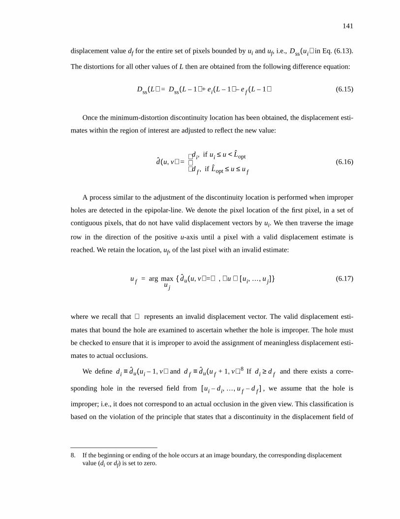
141
displacement valuedf for the entire set of pixels bounded byui anduf, i.e., in Eq. (6.13).
The distortions for all other values ofL then are obtained from the following difference equation:
(6.15)
Once the minimum-distortion discontinuity location has been obtained, the displacement esti-
mates within the region of interest are adjusted to reflect the new value:
(6.16)
A process similar to the adjustment of the discontinuity location is performed when improper
holes are detected in the epipolar-line. We denote the pixel location of the first pixel, in a set of
contiguous pixels, that do not have valid displacement vectors byui. We then traverse the image
row in the direction of the positiveu-axis until a pixel with a valid displacement estimate is
reached. We retain the location,uf, of the last pixel with an invalid estimate:
(6.17)
where we recall that represents an invalid displacement vector. The valid displacement esti-
mates that bound the hole are examined to ascertain whether the hole is improper. The hole must
be checked to ensure that it is improper to avoid the assignment of meaningless displacement esti-
mates to actual occlusions.
We define and .8 If and there exists a corre-
sponding hole in the reversed field from , we assume that the hole is
improper; i.e., it does not correspond to an actual occlusion in the given view. This classification is
based on the violation of the principle that states that a discontinuity in the displacement field of
8. If the beginning or ending of the hole occurs at an image boundary, the corresponding displacementvalue (di or df) is set to zero.
Dss ui( )
Dss L( ) Dss L 1–( ) ei L 1–( ) ef L 1–( )–+=
d u v,( )di if ui u Lopt<≤,
d f if Lopt u uf≤ ≤,
=
uf arg maxuj
du u v,( ) ∅= u∀ ui … uj, ,[ ]∈,{ }=
∅
di du ui 1– v,( )≡ d f du uf 1+ v,( )≡ di d f≥
ui di … uf d f–, ,–[ ]

142
one view corresponds to an occlusion in the other view, whose length, along an epipolar-line, is
equal to the magnitude of the discontinuity (see Section 3.2.2).
The improper hole in the displacement field is filled from Eq. (6.16) using an arbitrary bound-
ary between unoccluded regions. If , we use the previously described discontinuity adjust-
ment procedure to obtain the optimal location of the new unoccluded region boundary formed by
filling the hole.
This process of filling improper holes and adjusting the location of displacement discontinui-
ties is repeated until the entire image row has been traversed. The self-synthesis of the forward
field is complete when each row has been processed. The same procedure then is performed on the
reversed field.
The process of self-synthesis for a single image row is depicted in Fig. 6.5. The actual dis-
placement field and the estimated field after preprocessing are shown in Figs. 6.5a and 6.5b,
respectively. The various steps of the first pass that synthesizes View 0 from View 1 are shown in
Figs. 6.5(b)-(d), and the second pass is illustrated in Figs. 6.5(e)-(h). The adjusted and filled dis-
placement values are represented by the dashed lines after each step. We observe that the final,
processed field is identical to the actual field. While perfect reconstruction is unlikely in practice,
this scenario illustrates the capability of the self-synthesis technique to refine an estimated field,
provided that the initial field contains a sufficient number of accurate estimates.
6.3.2 Displacement Selection for Ambiguous Regions
Refining the displacement field through the self-synthesis process alleviates many of the displace-
ment errors that otherwise would have resulted in ambiguously-referenced regions in the interpo-
lated field. Nevertheless, inaccurate displacement estimates may still exist in the processed field.
We incorporate both range ordering and a measure of the reliability of an estimate to select the
proper displacement for pixels that are referenced by more than one vector.
We denote two displacement vectors that intersect at a pixel location in the interpolated field,
, by d1 andd2. We use the prediction block-SNR of each of these vectors, SNR1 and
SNR2, to quantify the reliability of the estimates. The SNR of a displacement estimate is calcu-
lated from the variance and prediction distortion of an image block in the decoded reference
di d f≠
dβ 0← u v,( )

143
View 1
View 0
View 1
View 0
View 1
View 0new locationof discontinuity
View 1
View 0
proper hole
a.
d.
c.
b.
Figure 6.5: Self-synthesis operation along single epipolar-line, (a) actualdisplacement field, (b)-(d) synthesis of View 0 from View 1, (e)-(g) synthesis of View1 from View 0, (h) final processed field.
ui uf
discontinuity
ui uf
di df
di df
u

144
e.
Figure 6.5: (cont.)
ui uf
di df
proper hole
View 1
View 0
f.
ui uf
di df
improper hole
View 1
View 0
g.
ui uf
di df
discontinuity
View 1
View 0
h.
ui uf
di df = 0
of discontinuitynew location
proper hole
View 1
View 0

145
frames. We include an additive term,q, to account for quantization noise introduced by the lossy
encoder:
(6.18)
where is the variance of the reconstructed image region (Eq. (2.11)), andD is the distortion
between the predicted and reconstructed block after residual decoding (Eq. (2.9)). The quantiza-
tion term is obtained from the characteristics of the residual encoder.
The selection of the displacement vector for the ambiguously-referenced pixel is given by,
(6.19)
whereTlow andThigh are user-specified thresholds that control the contribution of range ordering
and estimate reliability on the selection. If and , this scheme is equivalent to
the common approach of using only range ordering. If more than two displacement estimates inter-
sect at a single pixel in the interpolated field, a binary search is performed for the likely correct
estimate using Eq. (6.19).
6.3.3 Inferring Range Information for Occlusions
All holes remaining in the interpolated field are assumed to proper holes, i.e., they are due to
occlusions in the reference views. We assign displacement vectors to these regions based on
inferred range information for the occlusion. We again consider the case of two, horizontally-off-
set cameras, whereC0 is positioned to the left ofC1.
We assume that the scene has aregular structure, in that occluded regions have constant depth,
and that this depth is equal to the depth of the background unoccluded region adjacent to the occlu-
sion. While one can imagine situations were these assumptions are violated, our experience is that
the majority of real-world scenes have regular structures.
The interpolated field, , is traversed along each row. When a pixel is reached that
does not have a valid displacement estimate is reached, the initial location of the hole is noted (ui).
SNR σ2q+
D q+---------------=
σ2
dambig u v,( )d1 if
SNR1
SNR2-------------- Thigh or
SNR1
SNR2-------------- T low and d1 d2>>
>
,
d2 otherwise,
=
T low 0= Thigh ∞→
dβ 0← u v,( )

146
The final pixel location of this hole then is obtained from Eq. (6.17), which we have re-written for
convenience:
(6.20)
The displacements values on either side of the hole, and , are
examined to calculate the proper mapping for the hole and to resolve its visibility.
For the given camera geometry, the range of a scene object is related directly to its displace-
ment – the larger the displacement, the farther the object is from the camera pair. Therefore, the
background unoccluded region adjacent to the hole is the region with maximum displacement. We
assign pixels in the hole using,
(6.21)
Also, if , the geometry of the scene indicates that the occlusion was visible in View 0; oth-
erwise, it was visible in View 1. We mark each pixel in the hole as to in which view the region was
visible. This information is used in the final interpolation of the pixel intensity from Eq. (6.7).
A special case for this procedure occurs when one of the end-points of the hole is located at an
image border. If , we assign the displacementdf to the pixels in the hole. The visibility of
the occlusion is given by: visible in View 0 if , or visible in View 1 if . Appropriate
modifications are performed when the hole occurs at the right image border, i.e., .
Figure 6.6a depicts a simple scene consisting of three planar objects, in one dimension. The
perspective projection of an object for each view is given by the intersection the projection plane
with the projection from the object through the center of projection (camera lens). Interesting pro-
jections are drawn in the figure, where the objects have been shaded according to whether a partic-
ular portion is visible to one or both of the cameras. The tic-marks along the projection plane
represent pixels in the image frames.
The displacement field relating corresponding points in Views 0 and 1 for this sample scene is
shown in Fig. 6.6b. The interpolated field obtained by mapping unoccluded regions also is pro-
uf arg maxuj
du u v,( ) ∅= u∀ ui … uj, ,[ ]∈,{ }=
di du ui 1– v,( )≡ d f du uf 1+ v,( )≡
dhole u v,( )di if di d f>,
d f otherwise,
=
di d j>
ui 0=
d f 0< d f 0>
uf U 1–=

147
View 1
View 0b.
Object 1
Object 2
Object 3
Projectionplane
C0 C1
View β
View 1
View 0c.
View β
a.
Figure 6.6: Inferring range information for occluded regions, (a) perspective projectof sample scene, (b) field interpolated from unoccluded regions, (c) interpolated fieldafter filling occluded regions.
Object Key:Visible in both views
Visible in View 0
Visible in View 1
Cβ
148
vided, where the holes in the interpolated field are marked by the blackened pixels. Figure 6.6c
illustrates the results of the described algorithm – the dashed lines represent the inferred displace-
ment vectors for occluded regions. Since this scene has a regular structure, the inferred displace-
ment vectors corresponds exactly to the true object displacement.
6.4 Cost Analysis
In this section, we quantify the complexity and storage costs of our improved viewpoint interpola-
tion technique. When applicable, we make comparisons to the interpolation schemes described in
Section 6.2.
Before we provide our cost analysis, we make two observations on interpolation techniques.
The first observation is that the complete synthesis operation can be broken down into the distinct
steps of generating adense interpolated displacement vector field9, and interpolating pixel intensi-
ties using this field. All of the interpolation schemes known to the author perform the latter step in
roughly the same manner; therefore, we will not consider this process in our complexity compari-
sons. Secondly, many of the previously reported algorithms have not been developed in the context
of a complete multi-view encoder/decoder system; they do not indicate if the dense field is gener-
ated at the receiver or transmitter, and they do not consider the cost of transmitting the field if it
was estimated at the transmitter. To provide the most meaningful comparison, we will make rea-
sonable assumptions for the techniques that fail to mention these issues.
6.4.1 Complexity
Our technique generates the dense interpolated field by processing an initial displacement field,
obtained from a block-based procedure. Since we assume that the initial field is extracted from the
coded bit-stream, its calculation is essentially free, with respect to the interpolation operation. For
completeness, we denote the encoder complexity of our new algorithm by,
(6.22)
whereCBMA is the complexity of the block-matching algorithm, which is on the order of the dis-
placement estimation search range for a full-search technique.
9. The field is considered dense if it contains a displacement vector for each pixel location in theimage.
Cnew-encoder CBMA=

149
The initial field is processed at the decoder to: 1) eliminate likely false estimates (preprocess-
ing), 2) adjust the location of displacement discontinuities and fill improper holes (self-synthesis),
3) select the displacement for ambiguously-referenced pixels, and 4) fill proper holes by inferring
range information for occlusions. Except for the self-synthesis procedure, each of these steps
requires a fixed number of operations-per-pixel (see Table 6.1). The total decoder complexity of
the our method is:
(6.23)
whereCss represents the number of operations for the unidirectional self-synthesis procedure, and
the constant term equals the maximum number of operations for the steps with fixed complexity.
The complexity of the self-synthesis operation is difficult to analyze since it depends on the
number of discontinuities and improper holes in the initial field. Using Eq. (6.16) reduces the com-
plexity of locating the optimal unoccluded region boundary to a linear search over
. Experimental results indicate that both passes of the self-synthesis procedure
require an order of magnitude fewer operations than the full-search, block-based displacement
estimation step. This is particularly impressive since the search range for spatially-offset views is
one-dimensional. Our technique, therefore, is applicable to systems with a low-complexity
decoder constraint.
The EPI-based techniques generate the dense interpolated field using numerous, closely-
spaced views of the scene; the individual techniques used vary from nine [47] to 180 views [40].
Hence, we assume that the displacement field relating corresponding points within the extreme
views is generated at the encoder. The interpolated field is calculated at the decoder based on the
relative location of the desired viewpoint. The number of operations required to handle occlusions
Table 6.1: Average fixed complexity costs for the generation of interpolateddisplacement vector field.
Procedure Operations-per-pixel
Preprocessing 5
Unoccluded regions 4
Ambiguous regions < 1
Occluded regions < 1
Cnew-decoder 2Css 11+=
ui … uf 1+, ,[ ]
150
and ambiguously-referenced regions for each of these techniques are approximately equal to the
last three rows in Table 6.1, i.e., .
Hsu,et. al., use an edge detection and region growing procedure to estimate the displacement
field. Although the exact method was not described, region growing is typically considered a diffi-
cult (read computationally costly) procedure [40].
In [47], the interpolated field is generated by searching for the minimum variance trace line for
each pixel. To constrain the search, minimum and maximum trace line slopes are specified. For an
EPI containingM views, the per-pixel encoder complexity of this method is given by,
(6.24)
wheredmin anddmax at the relative locations of the end-points for the trace lines with the extre-
mum slope values.
The final EPI-based method of Fujii and Harashima requires an enormous search space for the
calculation of the triangular mesh grid points that yield the minimumVar-space. The authors did
not provide the search boundaries, so we cannot directly calculate the number of operations-per-
pixel; however, they did indicate the processing time required to perform their algorithm on a Sili-
con Graphics Iris Indigo Elan.10 Without theVar-space segmentation enhancement, fields for CIF-
sized images were obtained in “a few minutes”; with segmentation, the computational time was
“about 10 minutes” [30]. Obviously, this approach has excessive complexity.
The three-camera technique developed by Skerjanc and Liu generates the interpolated field
through: feature extraction, feature correspondence matching, and correspondence compatibility.
Due to the object-oriented (i.e., feature-based) approach, it is difficult to compute per-pixel com-
plexity quantities. Since each of these steps are performed in triplicate – once for each view or
pairs of views – we feel that this method is considerably more complex than our technique.
The technique presented by Thoma and Bierling is the most similar to our method in terms of
the partitioning of operations and complexity. An initial displacement field is obtained at the
encoder using a hierarchical block-matching algorithm (H-BMA):
(6.25)
10. Unfortunately, no mention of the processor or clock speed was given.
CEPI-decoder 6=
CKatayama-encoder 2M dmax dmin– 1+( )=
CThoma-encoder CH-BMA=

151
The field then is processed at the decoder to classify covered and uncovered regions using: change
detection, median filtering of a binary classification mask, and elimination of small regions. The
change detection and median filtering operations are sufficiently well described that we can calcu-
late the complexity of these steps; however, the explanation on how small regions are eliminated
was left somewhat open-ended. For the values provided in Table 3 of their work, the decoder com-
plexity is:
(6.26)
where is the number of operations-per-pixel to eliminate small regions and the constant
term is due to the change detection (9 operations), median filtering (13 operations), and mapping
of unoccluded pixels (4 operations).
Cafforio’s,et. al., method for motion-compensated interpolation performs a pel-recursive cal-
culation of the forward and backward displacement fields between temporally-offset frames. To
improve the robustness of the field, the recursion is performed four times for each field:
(6.27)
whereCpel-recur represents the number of operations-per-pixel for the pel-recursive analysis. Due
to the iterative process to generate the initial fields, we cannot assign a definitive quantity to this
variable. At the decoder, the bidirectional fields are processed to detect occluded regions and fill
pixels un-interpolated pels. Since the authors claim that only 2% of the pixels in the interpolated
field do not have valid displacement estimates, we will not include the filling of these pixels in the
complexity analysis. Finally, a 5-point median filter is applied to the interpolated field to ensure
spatial congruence in low detail areas. Assuming that the occlusion detection uses a window size
of pixels, the total complexity of the decoder is then,
(6.28)
which is broken down into: 9 operations for the occlusion detection, 4 operations for the mapping
of valid vectors, and 6 operations for the median filter.
CThoma-decoder CESR 26+=
CESR
CCafforio-encoder 8Cpel-recur=
3 3×
CCafforio-decoder 19=

152
The interpolation algorithm by Ribas-Corbera and Sklansky is very similar to that of Cafforio,
et. al. Here, bidirectional fields are generated at the encoder using optical flow analysis:
(6.29)
The fields then are analyzed at the decoder to detect occluded regions (using Cafforio’s searching
algorithm), and suppress gaps (holes) and ambiguities. The filling of gaps requires two compari-
sons, while ambiguities are handled through range ordering, i.e., a single comparison of the inter-
secting displacements. The total decoder complexity, including the mapping of unoccluded
displacements, is given by,11
(6.30)
In summary, our technique is substantially less complex than the EPI-based algorithms. While
our decoder requires slightly more operations than that of [13] or [83], our block-based displace-
ment field is encoded considerably more efficiently than their multiple, pixel-based fields; hence,
our approach is more applicable to viewpoint interpolation within a complete encoder/decoder
system.
6.4.2 Storage
At the encoder, our technique must store the two reference views and asparse displacement field.
The field is sparse since the displacement of each image block is described by a single vec-
tor.
At the decoder, additional frame memories are needed to store all of the desired intermediate
views. For the binocular motion parallax application, this amounts to a total of four frame stores –
two reference views and two interpolated views. We also require two dense displacement fields.
The first field relates corresponding pixels between Views 0 and 1, which is obtained by replicat-
ing the block vectors in the sparse field to each pixel, followed by the preprocessing and self-syn-
thesis operations. The second displacement field is the actual interpolated field used to predict the
11. The authors of this technique felt that the procedure presented by Thoma and Bierling was of“much higher complexity than [their] algorithm and Cafforio’s” [83]. In light of this discussion, webelieve this characterization is unjustified, unless the “elimination of small regions” in [93] consti-tutes a significant computational burden.
CRibas-Corbera-encoder 2Cflow=
CRibas-Corbera-decoder 16=
K L×

153
pixel intensities in the desired view. The data set for each pixel in these fields includes: a binary
flag indicating whether the pixel has a valid vector, along with the displacement vector and block-
SNR, if valid.
Our storage requirement is approximately equal to that of the various viewpoint interpolation
schemes that use only two views. Only our method requires SNR values for each valid vector.
Appropriate increases to the total storage cost are experienced if a technique uses bidirectional
fields [13, 83] or a change detection operator [93]. The other techniques that process more than
two views at the encoder require proportionally more storage based on the total number of views
[30, 40, 47, 89].
6.5 Experimental Results
The improved interpolation technique was used to synthesize intermediate viewpoints between
numerous views in the compressed multi-view sequences described in Section 2.4. The initial dis-
placement vector fields were extracted from the coded bit-stream that described the predictive cod-
ing of one of the reference views from the other. The reference views were predicted using a full-
search, block-based technique with full-pixel accuracy, where the displacement vectors were esti-
mated using an open-loop structure [68]. Block sizes of either or pixels were used,
depending on whether the view was a complete image frame or only a single field, i.e., sampled at
twice the frame rate. The reconstructed quality of the reference views was such that they were
indistinguishable from the original views.
For the self-synthesis operations, we used filter taps of and in
Eqs. (6.11) and (6.12). Also, the thresholds for the selection of ambiguously-referenced regions
were set to and . Nominally, all of the reference views were offset in
only their horizontal positions. Since exact camera alignment could not be guaranteed, we allowed
for some vertical displacement by slightly modifying our procedure to include deviations from the
epipolar-line constraint. The self-synthesis operation was still performed along scan-lines, but we
perturbed the locations of vertical displacement discontinuities to avoid long stretches of horizon-
tal holes.
The first results were obtained for theFlower Garden sequence. Although this is actually a
single-view sequence, the scene objects are stationary and the camera motion is almost completely
horizontal – two temporally-offset frames satisfy our camera geometry constraint. We illustrate the
interpolation results from using frames 0 and 3 as the reference views (Fig. 6.7). The major occlu-
16 16× 16 8×
h 1–( ) h 1( ) 1= = h 0( ) 2=
T low 0.95= T low 1.05=

154
sions in frame 0 are to the left of the large foreground tree and the left image border, and vice versa
for frame 3. The occluded portions are estimated to occupy roughly 7% of the image frames. The
true horizontal displacement in this pair of images was calculated to vary from 0 to 20 pixels.
Figure 6.8 illustrates the horizontal component of the displacement fields relating frames 0 and
3 after the various processing steps of our algorithm. We observe the poorly delineated object
boundaries and improper holes in the preprocessed field. After self-synthesis of frame 0 from
frame 3, Fig. 6.8b, the displacement discontinuity along the right side of the tree closely matches
the true object boundary. Similar refinement for the left side of the tree is obtained from the second
self-synthesis pass; the blockiness of the initial field is completely eliminated.
The blackened pixels in the displacement fields represent pixels assumed to be occluded. The
corresponding pixels in the original frames have been blackened in Fig. 6.9 to examine the perfor-
mance of this method to detect occlusion. The major occlusions are accurately localized. Most of
the spurious invalidated pixels are due to displacement errors in regions with uniform intensity,
e.g., the sky, and should not detract from the subjective quality of the interpolated views.
Frame 1 was interpolated using the processed field by setting . The interpolated view is
virtually indistinguishable from the original (Fig. 6.10). Accurate synthesis of the image borders
and sides of the foreground tree were obtained, and a PSNR of over 28 dB was measured.12 This
represents an improvement of over 3.5 dB from our earlier work [63], which did not include the
preprocessing and self-synthesis steps. Fujii and Harashima reported only 17 dB for the interpola-
tion of a similar frame in this sequence [30].13 The absolute frame difference from using the repiti-
tion of frame 0 and our interpolation technique for this image are shown in Fig. 6.11. The frame
repitition results indicate that a majority of the image is displaced between frames.
For comparison, we interpolated this frame using the unprocessed, block-based displacement
field, where the displacement of ambiguously-referenced pixels were chosen based solely on range
ordering (Fig. 6.12a). Since the common assumption of zero displacement for holes in the interpo-
lated field is violated for spatially-offset views, we filled these holes by using our method of infer-
ring range information for occluded regions. We observe very poor reconstruction of the image
borders and the regions surrounding the foreground tree. We also include the results of performing
12. We note that even better performance could have been obtained if we were provided with the exactcamera motion between frames, as opposed to the assumed motion – calculation of the exact epipo-lar-line would be possible and the relative location of the intermediate frames would be known.
13. The authors did not distinguish between SNR and PSNR in their work. Based on the subjectivequality of the reconstructed image, we feel that the 17 dB quantity represented PSNR.
β 13---=

155
a bidirectional block-based prediction of this frame using frame 0 and 3 as the reference frames in
Fig. 6.12b. While the PSNR of this image is comparable to the interpolated view using our
improved technique, the subjective quality of the interpolated image is far superior. Also, over
4000 bits are required to describe the bidirectionally-predicted image, while no bits need to be
transmitted for the interpolated view.
The results obtained for the interpolation of frame 2, , are illustrated in Figs. 6.13-6.15.
The same procedure was performed for the entire Flower Garden sequence, where the reference
views were offset by three frames, i.e., 3:1 temporal subsampling. The average PSNR for the inter-
polated views was approximately 27.5 dB. The interpolation was simulated in C on a Silicon
Graphics workstation with a single R4400, 174 MHz processor. Each interpolated displacement
vector field was generated in less than 1.5 seconds.
A total of sixty views, obtained from the interpolation of 20 views between each of first three
pairs of reference views, have been used extensively in a binocular multi-view display system. A
head-tracking device is used to display the appropriate stereo-pair based on the viewer’s horizontal
position, and a “stereo-dial” allows viewers to specify the inter-camera separation. Although some
regions of the interpolated views exhibit inconsistent object displacement due to unrectified errors
in the displacement field, viewers report effective motion parallax and diminished eye strain with
this system.
The second result that we will examine is the viewpoint interpolation of the two-viewVolley-
ball sequence. The original 155th frames for each view of this sequence are shown in Fig. 6.16. We
observe that the reference views are very similar – occluded regions are almost totally non-existent
and when an occlusion does exist it has uniform intensity, e.g., the occlusions between the players
and the ground. We manually calculated the true range of the horizontal displacement to equal 14
pixels.
Interpolation of the viewpoint located halfway between the reference views was performed
using our improved technique and a basic interpolation scheme (Fig. 6.17). The basic interpolator
uses the unprocessed, block-based displacement field, selects the displacement for ambiguous
regions using range ordering, and assigns zero displacement to holes in the interpolated field using
the technique described in [83]. Both methods achieve subjectively-pleasing interpolated views for
this sequence. These results indicate that the basic interpolator is sufficient for scenes with rela-
tively simple structures and limited occlusion. The real advantage of our improved technique is
evident for more complex scenes, as illustrated for the following sequence.
β 23---=

156
Numerous intermediate views were synthesized between Views 1 and 2 of theCement Mixer
sequence.14 We will examine the results for the 175th frame, where the original images are illus-
trated in Fig. 6.18. Large occlusions exist on either side of the foreground tree and image borders,
and the scene objects are located at numerous depth planes; less obvious occlusions are present
surrounding the person located between the cars and truck. The occluded portions are estimated to
occupy roughly 10% of the reference views. The horizontal displacement range was estimated to
be over 50 pixels, which is substantially greater than any scene used to evaluate prior interpolation
techniques known to the author.
The intermediate viewpoints, , obtained from using our technique are shown in
Figs 6.19, 6.20, and 6.21, respectively. While visual artifacts are present, we feel that these inter-
polated views are quite impressive given the complexity of the scene. In particular, the image bor-
ders are faithfully reconstructed and appropriate regions behind the foreground tree become visible
asβ varies; e.g., the entire ladder is visible inF(1.75,175), but only a portion of it can be seen in
F(1.25.175).
We compare these results with those obtained by the basic interpolator by eliminating various
enhancements from our procedure. The interpolated view shown in Fig. 6.22 was generated using
the initial, unprocessed displacement vector field. Ambiguous regions and holes in the interpolated
field were handled using our method. The right image border is poorly interpolated, and objection-
able block artifacts are present throughout the intermediate view. The next comparison was made
by interpolating the same viewpoint using the displacement field after preprocessing and self-syn-
thesis, but without our ambiguous regions selection and occlusion filling procedures (Fig. 6.23).
The blockiness of the previous scheme is eliminated, but artifacts resembling speckle noise now
exist at object boundaries. Also, many of the regions in the interpolated view do not correspond to
the true geometry of the scene; the end of the cement chute is visible on the right side of the tree
and the majority of the ladder is missing. These errors are due to the improper assumption of zero
displacement for holes in the interpolated field. Figure 6.24 illustrates the interpolation perfor-
mance of the basic scheme that does not include any of our enhancements. This unsatisfactory
intermediate view is plagued by both blockiness and incorrect scene geometry.
The final results obtained for thePiano sequence illustrate the subtleties of our enhanced inter-
polation scheme. The original 25th frame for Views 0 and 1 of this sequence are shown in Fig.
14. The interpolation of viewpoints between Views 0 and 1 of this sequence were not performed sincethe respective foci were so poorly aligned.
β 14--- 1
2--- 3
4---, ,=

157
6.25. While there is a moderate amount of object depth discontinuity, the majority of occlusions
are regions of uniform intensity, e.g., the background surrounding the person’s head. For a more
interesting occlusion, we direct the reader to examine the lower-left corner ofF(0,25), where a
portion of the flower arrangement is occluded by the piano player.
The interpolated viewpoints, located at , obtained from using our enhanced scheme and
the basic scheme are shown in Fig. 6.26. Both of these techniques provide subjectively-pleasing
results for a majority of the image. Upon closer examination, though, we observe the superiority of
our technique. Figure 6.27 contains close-ups of the lower-left corner of the reference and interpo-
lated views. The object to the left of the person, which is only partially visible inF(1,25), is accu-
rately reconstructed in Fig. 6.27b. While such improvements appear minor when viewing
individual frames, they are significant when the interpolated views are used in the motion parallax
and viewer-specified camera separation applications to ensure object continuity.
6.6 Summary
In this chapter, we have presented an improved displacement-compensated interpolation scheme.
The interpolation problem was considered in the context of a complete multi-view encoder/
decoder system, capable of providing the viewer with simulated motion parallax and control over
the perceived depth range in the imagery. To ensure compliance with current predictive coding
standards, the interpolation was performed using a single, noisy displacement vector field obtained
from a conventional block-based displacement estimation technique.
Errors traditionally associated with block-based displacement estimation schemes were
reduced through a preprocessing step to eliminate likely false estimates and a self-synthesis proce-
dure to refine displacement discontinuities and fill improper holes. By using the initial field as a
guide as to how the field may be adjusted, pixel-based accuracy for unoccluded region boundaries
and occlusions were obtained via the self-synthesis operation with minimal computational com-
plexity.
Pixels assumed to be unoccluded in the processed displacement field were mapped to the inter-
mediate image using the geometric relationship between the views. We used a combination of both
range ordering and a displacement estimation confidence measure to handle the situation when a
pixel in the intermediate view was mapped by more than one reference image pixel. Un-interpo-
lated pixels were assumed to be due to occlusions in the reference views. To fill these pixels, we
inferred range information for occlusions based on a regular-scene-structure assumption.
β 12---=

158
Interpolation results for numerous multi-view signals were presented. Our technique synthe-
sized subjectively-pleasing intermediate views from reference views with moderate to high per-
centages of occlusions, and required relatively low complexity and storage costs. For the one
sequence were the actual intermediate views were available, our improved method achieved an
average PSNR of approximately 27.5 dB without requiring any additional bit rate beyond that
needed to encode the two reference views. These results validate our claim that satisfactory inter-
polation is possible from only two spatially-offset views.
Future work includes incorporating additional image information into the self-synthesis proce-
dure to further improve the localization of displacement discontinuities and occlusions. This may
entail the integration of edge and color information into the optimal boundary cost function.

159
Figure 6.7:Flower Garden, (a) original frame 0, (b) original frame 3
a.
b.

160
Figure 6.8: Estimated displacement fields (horizontal component) after variousprocessing stages. Left column: frame 0 from frame 3. Right column: frame 3 fromframe 0. (a) after thresholding, border elimination and field reversal, (b) after self-synthesis of frame 0, (c) after self-synthesis of frame 3.
a.
c.
b.

161
Figure 6.9: Occlusion localization results, (a) frame 0, (b) frame 3.
a.
b.

162
Figure 6.10:Flower Garden frame 1, (a) original, (b) interpolated.
a.
b.

163
Figure 6.11: Absolute frame difference for frame 1, (a) frame repetition,PSNR=15.72 dB, (b) interpolation, PSNR=28.14 dB.
a.
b.

164
Figure 6.12: Flower Garden frame 1, (a) interpolated without performingdisplacement field processing and ambiguous region selection (PSNR=24.54 dB),(b) bidirectionally-predicted from reference frames 0 and 3 using a fixed-size,block-based technique (PSNR= 28.55 dB).
a.
b.

165
Figure 6.13:Flower Garden frame 2, (a) original, (b) interpolated.
a.
b.

166
Figure 6.14: Absolute frame difference for frame 2, (a) frame repetition,PSNR=15.85 dB, (b) interpolation, PSNR=28.00 dB.
a.
b.

167
Figure 6.15: Flower Garden frame 2, (a) interpolated without performingdisplacement field processing and ambiguous region selection (PSNR=24.86 dB),(b) bidirectionally-predicted from reference frames 0 and 3 using a fixed-size,block-based technique (PSNR= 28.89 dB).
a.
b.

168
Figure 6.16:Volleyball, (a) originalF(0,155), (b) originalF(1,155)
a.
b.

169
Figure 6.17: Volleyball F(0.5,155), (a) interpolated using enhancements, (b)interpolated without enhancements.
a.
b.

170
Figure 6.18:Cement Mixer, (a) originalF(1,175), (b) originalF(2,175)
a.
b.

171
Figure 6.19:Cement Mixer F(1.25,175) interpolated using improved technique.

172
Figure 6.20:Cement Mixer F(1.5,175) interpolated using improved technique.

173
Figure 6.21:Cement Mixer F(1.75,175) interpolated using improved technique.

174
Figure 6.22: Cement Mixer F(1.5,175) interpolated without displacement fieldprocessing.

175
Figure 6.23: Cement Mixer F(1.5,175) interpolated using range ordering forambiguously-referenced image regions and zero displacement occlusion filling.

176
Figure 6.24: Cement Mixer F(1.5,175) interpolated using unprocessed field, rangeordering for the selection of ambiguously-referenced image regions, and filling ofholes with zero displacement.

177
Figure 6.25:Piano, (a) originalF(0,25), (b) originalF(1,25)
a.
b.

178
Figure 6.26: Piano F(0.5,25), (a) interpolated using improved technique, (b)interpolated using basic scheme.
a.
b.

179
Figure 6.27: Close-ups ofPiano frame, (a) originalF(0,25), (b) interpolatedF(0.5,25) using improved technique (c) interpolatedF(0.5,25) using basicinterpolation scheme, (d) originalF(1,25)
a.
c.b.
d.

180
Chapter 7
Conclusions and Future Work
In this thesis, we addressed the problem of efficiently compressing multiple, concurrent views of a
scene, obtained from cameras arranged in an arbitrary (non-periodic) configuration. The underly-
ing concept behind this work is that single-view video signal characteristics, typically exploited by
coding algorithms, do not necessarily apply to multi-view signals. For example, in these signals: 1)
the relative location of the optimal reference frame depends on the structure and motion of both
scene objects and cameras, 2) significant correlation exists between the predicted and residual
images due to lighting and camera pick-up variations, and 3) most scene objects possess non-zero
displacement between frames within separate views. We developed three distinct algorithms that
utilized the special characteristics of multi-view signals with the goal of achieving superior rate-
distortion performance while maintaining acceptable complexity and storage costs.
Improved frame-based prediction was achieved by a simple method to adaptively select the
best possible reference for the frame to be encoded. The selection was based on the adverse effect
of occlusions on prediction performance, and the one-to-one relationship between occlusions and
discontinuities within a displacement vector field. For constant quality reconstructed images, this
technique realized a bit rate reduction of 10-30% when compared with fixed, pre-selected refer-
ence frame schemes; it also achieved rate-distortion performance within 1% of an exhaustive
search method, while consuming considerably fewer processing cycles. These gains were offset by
a storage requirement approximately 2-3 times that of the fixed or exhaustive search methods.
A novel class of residual encoders was presented that is capable of exploiting correlation
between the predicted and residual images. The functionality of this coder resembles that of a pre-
dictive vector quantizer, with the significant difference that a unique vector predictor is associated
with each reproduction vector. This explicit coupling allows for the tracking of non-stationarities
in the source signal without the transmission of side information; it also provides for the joint opti-
mization of the predictor and quantizer. For fixed average distortion, this technique required

181
roughly 15% fewer bits compared with a comparable vector quantizer; for a constant bit rate of
approximately 0.13 bpp, the average gain in signal-to-noise ratio was over 0.8 dB. Unfortunately,
these gains were obtained at the expense of high encoder complexity and storage costs.
An enhanced viewpoint interpolation scheme was developed, which requires the use of only
two decoded exterior views and the noisy, block-based, displacement vector field extracted from
the coded bit stream relating these views. Problems typically encountered in interpolation schemes
were minimized by: rectifying displacement estimation errors, due to displacement discontinuities
within an image block, via the self-synthesis procedure; inferring range information for occlusions
from neighboring unoccluded regions; and selecting the correct displacement for ambiguously-ref-
erenced regions by using a displacement estimate confidence measure. This technique was applied
to numerous stereo-pairs, and subjectively-pleasing intermediate views were obtained; impressive
results were realized even for image pairs with relatively large displacement ranges.
A summary of the relative costs for our novel reference frame selection, residual encoding,
and viewpoint interpolation algorithms are provided in Tables 7.1, 7.2, and 7.3, respectively. The
cost values were obtained from the simulations performed on our set of multi-view signals, and
they were normalized with respect to the corresponding baseline technique. Definitions of these
costs are provided in Section 2.3, where we used the mean-squared-error distortion function, and
measured complexity in terms of the processing time to perform each technique.
Figure 7.1 illustrates a complete multi-view hybrid coder structure that incorporates all three
of these algorithms. We observe that any or all of these techniques may be employed. With respect
to overall system cost, we reach the following conclusions. If encoder storage is not a concern,
adaptive reference frame selection should be performed – the rate-distortion performance afforded
by this technique far outweighs it relatively moderate complexity cost. Only in systems that have
severe bit rate constraints should the restoration-based coder be utilized – more substantial
improvements will need to be observed, on diverse multi-view signals, for this technique to over-
come its complexity and storage requirements. Finally, due to its superior performance and mini-
mal costs, interior views should not be generated, and, instead, viewpoint interpolation should be
performed at the decoder.
Besides the future work described for each algorithm in their respective chapter summaries,
we plan on applying these techniques to more elaborate multi-view signals, i.e., number of views
greater than two. The techniques that prove most useful then should be implemented into a real-
time, multi-view communication system possessing the desirable features of simulated motion
parallax and viewer-specified level of stereoscopy.

182
Table 7.1: Relative encoder cost comparison summary between fixed, exhaustive, andadaptive reference frame selection schemes.
Technique Rate Distortion Complexity Storage
Fixed 1.00 1.00 1.00 1.00
Exhaustive 0.79 1.00 3.83 1.00
Adaptive 0.78 1.00 2.40 2.06
Table 7.2: Relative encoder cost comparison summary between vector quantization(PTSVQ) and vector restoration (PTSVR) residual encoder implementations.
Technique Rate Distortion Complexity Storage
PTSVQ 1.00 1.00 1.00 1.00
PTSVR 0.87 0.99 3.12 1.37
Table 7.3: Relative decoder cost comparison summary between basic and enhancedviewpoint interpolation techniques.
Technique Rate Distortion Complexity Storage
Basic 1.00 1.00 1.00 1.00
Enhanced 1.00 0.58 1.32 1.39

183
Figure 7.1: Complete multi-view hybrid coder structure incorporating adaptivereference frame selection, restoration-based residual coding, and viewpointinterpolation from a noisy displacement vector field.
Prediction description
Decoding description (transmit)Original image
Reconstructed image
ENCODER
Adaptive
Restoration-basedResidual Encoding
ResidualDecoding
ReferenceSelection
FrameMemories
Predicted image
Decoding
Reconstructed
DECODER
FramePrediction
FrameMemories
Predicted
description ViewpointInterpolator
Relative reference
image
image
ResidualDecoding
Interpolatedimage
+
+
+
-
+
+
Prediction description
FramePrediction
(transmit)
frame location
Relative referenceframe location (transmit)

184
Bibliography
[1] CCITT Study Group XV - Report R95, Recommendation H.261, “Video Codec for Audiovi-sual Services at p x 64 kbits,” May 1992.
[2] ISO/IEC JTC1/SG29/WG11, ISO/IEC 11172-2, “Information Technology - Coding of mov-ing pictures and associated audio for digital storage media at up to about 1.5 Mbits/s - Part 2:Video”, May 1993.
[3] ISO/IEC JTC1/SC29/WG11 Test Model Editing Committee, “MPEG-2 Video Test Model5", ISO/IEC JTC1/SC29/WG11 Doc. N0400, April 1993.
[4] ISO/IEC JTC1/SC29/WG11, “Information Technology - Generic Coding of Moving Picturesand Associated Audio, Recommendation H.262, ISO/IEC 13818-2, Draft International Stan-dard,” March 1994.
[5] G. P. Abousleman, M. W. Marcellin and B. R. Hunt, “Compression of hyperspectral imageryusing the 3-D DCT and hybrid DPCM/DCT,”IEEE Trans. Geoscience and Remote Sensing,vol. 33, no. 1, pp. 26-34, Jan. 1995.
[6] A. Asif and J. M. F. Moura, “Image codec by noncausal prediction, residual mean removal,and cascaded VQ,”IEEE Trans. on Circuits and Systems for Video Tech., vol. 6, no. 1, pp.42-55, Feb. 1996.
[7] H. Aydinoglu and M. H. Hayes, “Compression of multi-view images,” inProc. IEEE Int.Conf. Image Processing, vol. 2, pp. 385-389, Nov. 1994.
[8] N. Balram and J. M. F. Moura, “Noncausal Gauss Markov random fields: Parameter struc-ture and estimation,”IEEE Trans. Inform. Theory, vol. 38, no. 2, pp. 334-354, Mar. 1993.
[9] H. H. Baker and R. C. Bolles, “Generalizing epipolar plane image analysis on the spatiotem-poral surface,”Int. J. of Computer Vision, vol. 3, no. 1, pp. 33-49, 1989.
[10] S. T. Barnar and M. A. Fischler, “Disparity analysis of images,”IEEE Trans. Pattern Anal.Machine Intell., vol. 2, pp. 333-340, July 1980.
[11] R. C. Bolles, H. H. Baker and D. H. Marimont, “Epipolar-plane image analysis: An approachto determining structure from motion,”Int. J. of Computer Vision, vol. 1, no. 1, pp. 176-185,1987.

185
[12] L. Breiman, J. H. Friedman, R. A. Olshen and C. J. Stone,Classification and RegressionTrees. The Wadsworth Statistics / Probability Series, Belmont CA: Wadsworth, 1984.
[13] C. Cafforio, F. Rocca and S. Tubaro, “Motion compensated image interpolation,”IEEETrans. Comm., vol. 38, no. 2, pp. 215-222, Feb. 1990.
[14] E. Chalom, E. and V. M. Bove, V.M, “Segmentation of frames in a video sequence usingmotion and other attributes,” inProc. Digital Video Compression: Algorithms and Technolo-gies 1995, SPIE, vol. 2419, pp. 230-241, 1995.
[15] R. Chassaing, B. Choquet and D. Pele, “A stereoscopic television system (3D-TV) and com-patible transmission on a MAC channel (3D-MAC)”,Signal Processing: Image Communica-tion, vol. 4, no. 1, pp. 33-43, Nov. 1991.
[16] P. A. Chou, T. Lookabaugh and R. M. Gray, “Optimal pruning with application to tree-struc-tured source coding and modeling,”IEEE Tran. Inform. Theory, vol. 35, no. 2, pp. 299-315,1989.
[17] P. A. Chou, T. Lookabaugh and R. M. Gray, “Entropy-constrained vector quantization,”IEEE Trans. Acoust., Speech, Signal Processing, vol. 37, no. 1, pp. 31-42, 1989.
[18] R. J. Clarke,Transform Coding of Images, London: Academic Press, 1985.
[19] L. Corte-Real and A. P. Alves, “A very low bit rate video coder based on vector quantiza-tion,” IEEE Trans. Image Processing, vol. 5, no. 2, pp. 263-273, Feb. 1996.
[20] J. L. Crowley, P. Bobet and C. Schmid, “Auto-calibration by direct observation of objects,”Image and Vision Computing, vol. 11, no. 2, pp. 67-81, Mar. 1993.
[21] G. Demoment, “Image reconstruction and restoration: Overview of common estimationstructures and problems,”IEEE Trans. Acoust., Speech, Signal Processing, vol. 37, no. 12,pp. 2024-2036, Dec. 1989.
[22] I. Dinstein, M. G. Kim, A. Henik and J. Tzelgov, “Compression of stereo images using sub-sampling and transform coding,”Optical Engineering, vol. 30, no. 9, pp. 1359-1364, Sept.1991.
[23] I. Dinstein, G. Guy, J. Rabany, J. Tzelgov and A. Henik, “On the compression of stereoimages: Preliminary results,”Signal Processing, vol. 17, no. 4, pp. 373-382, Aug. 1989.
[24] M. Effros and P. A. Chou, “Weighted universal transform coding: Universal image compres-sion with the Karhunen-Loève Transform,” inProc. IEEE Internat. Conf. Image Processing,vol. 2, pp. 61-64, 1995.
[25] D. Eggert and K. Bowyer, “Computing the perspective projection aspect graph of solids ofrevolution,” IEEE Trans. Pattern Analysis and Machine Intelligence, vol. 15, no. 2, pp. 109-128, 1993.
[26] N. Farvardin and J. W. Modestino, “Rate-distortion performance of DPCM schemes forautoregressive sources,”IEEE Trans. Inform. Theory, vol., 31, no. 3, pp. 402-418, May 1985.

186
[27] J. D. Fooley,Introduction to Computer Graphics,Reading, MA: Addison-Wesley, 1994.
[28] M. Foodeei and E. Dubois, “Coding image sequence intensities along motion trajectoriesusing EC-CELP quantization,” inProc. IEEE Int. Conf. Image Processing, pp. 720-724,1994.
[29] M. Foodeei and E. Dubois, “Rate-distortion performance of source coders in the low bit-rateregion for highly correlated Gauss-Markov source,” inProc. GLOBECOM, pp. 123-127,1993.
[30] T. Fujii and H. Harashima, “Data compression of an autostereoscopic 3-D image,” Univer-sity of Tokyo Tech. Rep., 1994.
[31] B. Gerod, “The efficiency of motion-compensating prediction for hybrid coding of videosequences,”IEEE J. Select. Areas Commun., vol. 5, pp. 1140-1154, Aug. 1987
[32] A. Gersho and R. Gray,Vector Quantization and Signal Compression, Boston: Kluwer Aca-demic, 1991.
[33] V. S. Grinberg, G. Podnar and M. W. Siegel, “Geometry of binocular imaging,” inProc. Ste-reoscopic Displays and Virtual Reality Systems, SPIE, vol. 2177, pp. 56-65, 1994.
[34] E. Grosso and M. Tistarelli, “Active/dynamic stereo vision,”IEEE Trans. on Pattern Analysisand Machine Intelligence, vol. 17, no. 9, pp. 868-879, Sept. 1995.
[35] S. Gupta and A. Gersho, “Feature predictive vector quantization of multispectral images,”IEEE Trans. Geoscience and Remote Sensing, vol. 30, no. 3, pp. 491-501, May 1992.
[36] S. Gupta and A. Gersho, “Nonlinear predictive vector quantization of multispectral imag-ery,” in Proc. Twenty-Fourth Asilomar Conf. Signals, Systems and Computers, pp. 331-335,1990.
[37] C. Hansen, N. Ayache and F. Lustman, “Efficient depth estimation using trinocular stereo,”in Proc. Sensor Fusion: Spatial Reasoning and Scene Interpretation, Cambridge, MA, SPIE,vol. 1003, pp. 124-131, 1988.
[38] R. Hopkins, “Digital terrestrial HDTV for North America: The Grand Alliance HDTV sys-tem,”, IEEE Trans. Consumer Electronics, vol. 40, no. 3, pp. 185-198, Aug. 1994.
[39] C.-H. Hsieh and J.-S. Shue, “Frame adaptive finite-state vector quantization for imagesequence coding,”Signal Processing: Image Communication, vol. 7, pp. 13-26, 1995.
[40] R. Hsu, K. Kodama and H. Harashima, “View interpolation using epipolar plane images,” inProc. IEEE Int. Conf. Image Processing, vol. 2, pp. 745-749, 1994.
[41] C.-L. Huang and T.-T. Chao, “Motion-compensated interpolation for scan rate up-conver-sion,” Optical Engineering, vol. 35, no. 1, pp. 166-176, Jan. 1996.
[42] A. K. Jain,Fundamentals of Digital Image Processing, Englewood Cliffs NJ: Prentice Hall,1989.

187
[43] A. K. Jain, “Advances in mathematical models for image processing,”Proc. IEEE, vol. 69,no. 5, pp. 502-528, May 1981.
[44] J. R. Jain and A. K. Jain, “Displacement measurement and its application in interframeimage coding,”IEEE Trans. Comm., vol. 29, pp. 1799-1808, Dec. 1981.
[45] B. Julesz,Foundations of Cyclopean Perception, Chicago: The University of Chicago Press,1971.
[46] T. Kanade and M. Okutomi, “A stereo matching algorithm with an adaptive window: Theoryand experiment,” inProc. Int. Conf. Robotics and Automation, pp. 1088-1095, 1991.
[47] A. Katayama, K. Tanaka, T. Oshino and H. Tamura, “A viewpoint dependent stereoscopicdisplay using interpolation of multi-viewpoint images,” inProc. Stereoscopic Displays andVirtual Reality Systems II, SPIE, vol. 2409, pp. 11-20, 1995.
[48] J.-S. Kim and R.-H. Park, “Local motion-adaptive interpolation technique based on blockmatching algorithms,”Signal Processing: Image Communications, vol. 4, no. 6, pp. 519-528, Nov. 1992.
[49] Y. Kim, I. Choi, I. Lee, T. Yun, and K. T. Park, “Wavelet transform image compression usinghuman visual characteristics and a tree structure with a height attribute,”Optical Engineer-ing, vol. 35, no. 1, pp. 204-212, Jan. 1996.
[50] Y. H. Kim and J. W. Modestino, “Adaptive entropy-coded pruned tree-structured predictivevector quantization of images,”IEEE Trans. Comm., vol. 41, no. 1, Jan. 1993.
[51] B. Kost and S. Pastoor, “Visibility thresholds for disparity quantization errors in stereoscopicdisplays,”Proc. SID, vol. 32, no. 2, pp. 165-170, 1991.
[52] E. Krotkov, M. Hebert and Simmons, “Stereo perception and dead reckoning for a prototypelunar rover,”Autonomous Robots, vol. 2, no. 4, pp. 313-331, 1995.
[53] D. Kundur and D. Hatzinakos, “Blind image deconvolution,”IEEE Signal Processing Mag.,vol. 13, no. 3, pp. 43-64, May 1996.
[54] Y. Linde, A. Buzo and R. M. Gray, “An algorithm for vector quantization design,”IEEETran. Comm., vol. 28, no. 1, pp. 84-95, 1980.
[55] L. Lipton, The CrystalEyes Handbook, San Rafael CA: StereoGraphics Corporation, 1991.
[56] J. Liu and R. Skerjanc, “Stereo and motion correspondence in a sequence of stereo images,”Signal Processing: Image Communication, vol. 5, pp. 305-318, 1993.
[57] C. Loeffler, A. Ligtenberg and G. Moschytz, “Practical fast 1-D DCT algorithms with 11multiplications,” inProc. Int. Conf. Acoust., Speech, Signal Processing, pp. 988-991, 1989.
[58] T. Lookabaugh, E. A. Riskin, P. A. Chou and R. M. Gray, “Variable rate vector quantizationfor speech, image, and video compression,”IEEE Trans. Comm., vol. 41, no. 1, pp. 186-199,Jan. 1993.

188
[59] M. E. Lukacs, “Predictive coding of multi-viewpoint image sets,” inProc. IEEE Int. Conf.Acoust., Speech, Signal Processing, vol. 1, pp. 521-524, 1986.
[60] J. N. Mailhot and H. Derovanessian, “Grand Alliance HDTV video encoder,”IEEE Trans.Consumer Electronics, vol. 41, no. 4, pp. 1014-1019, Nov. 1995.
[61] F. C. M. Martins and J. M. F. Moura, “3-D video compositing: Towards a compact represen-tation for video sequences,” inProc. IEEE Int. Conf. Image Processing, pp. 550-553, 1995.
[62] T. Miyashita and T. Uchida, “Cause of fatigue and its improvement in stereoscopic displays,”Proc. SID, vol. 31, no. 3, pp. 249-254, 1990.
[63] J. S. McVeigh, M. W. Siegel and A. G. Jordan, “Intermediate view synthesis consideringoccluded and ambiguously referenced image regions,”Signal Processing: Image Communi-cations, accepted.
[64] J. S. McVeigh, M. W. Siegel and A. G. Jordan, “Adaptive reference frame selection for gen-eralized video signal coding,” inProc. Digital Video Compression: Algorithms and Technol-ogies 1996, SPIE, vol. 2668, pp. 441-449, 1996.
[65] J. S. McVeigh, M. W. Siegel and A. G. Jordan, “Algorithm for automated eye-strain reduc-tion in real stereoscopic images and sequences,” inProc. Human Vision and ElectronicImaging, SPIE, vol. 2657, pp. 307-316, 1996.
[66] J. S. McVeigh, S.-W. Wu, M. W. Siegel and A. G. Jordan, “Vector restoration for video cod-ing,” in Proc. IEEE Int. Conf. Image Processing, vol. 1, pp. 93-96, 1995.
[67] J. S. McVeigh, V. S. Grinberg and M. W. Siegel, “Double buffering technique for binocularimaging in a window,” inProc. Stereoscopic Displays and Virtual Reality Systems II, SPIE,vol. 2409, pp. 168-175, 1995.
[68] J. S. McVeigh and S.-W. Wu, “Partial closed loop versus open loop motion estimation forHDTV compression,”Int. J. Imaging Systems and Technology, vol. 5, no. 4, pp. 268-275,1994.
[69] N. M. Nasrabadi, C. Y. Choo and Y. S. Feng, “Finite-state vector quantization of digitalimages,”IEEE Trans. Comm., vol. 32, no. 5, pp. 2145-2154, May 1994.
[70] A. Ortega and M. Vetterli, “Adaptive quantization without side information,” inProc. IEEEInt. Conf. Image Processing, vol. 3, pp. 856-860, 1994.
[71] K. K. Pang and T. K. Tan, “Optimum loop filter in hybrid coders,”IEEE Trans. Circuits andSystems for Video Tech., vol. 4, no. 2, pp. 158-167, Apr. 1994.
[72] S. Panis and M. Ziegler, “Object-based coding using motion and stereo information,” inProc. Picture Coding Symposium, pp. 308-312, 1994.
[73] A. Papoulis,Probability, random variables, and stochastic processes, New York: McGraw-Hill, 1991, ch. 12.

189
[74] S. Pastoor, “3D-television: A survey of recent research results on subjective requirements,”Signal Processing: Image Communication, vol. 4, no. 1, pp. 21-32, Nov. 1991.
[75] S. Pastoor and K. Schenke, “Subjective assessments of the resolution of viewing directionsin a multi-viewpoint 3D TV system,”Proc. SID, vol. 30, no. 3, pp. 217-223, 1989.
[76] M. G. Perkins, “Data compression of stereopairs,”IEEE Trans. Comm, vol. 40, no. 4, pp.684-696, Apr. 1992.
[77] A. Puri and B. Haskell, “Straw man proposal for multi-view profile,” ISO/IEC JTC1/SC29/WG11 MPEG95/485, Nov. 1995.
[78] A. Puri, R. V. Kollarits and B. G. Haskell, “Stereoscopic video compression using temporalscalability,” in Proc. Visual Communications and Image Processing, SPIE, vol. 2501, pp.745-756, 1995.
[79] R. L. de Queiroz and K. R. Rao, “Variable block size lapped transforms,” inProc. IEEE Int.Conf. Image Processing, vol. 2, pp. 290-293, 1995.
[80] K. R. Rao and P. Yip,Discrete Cosine Transform - Algorithms, Advantages, Applications,London: Academic Press, 1990, appendix A.2.
[81] C. Reader, “MPEG4: coding for content, interactively, and universal accessibility,”OpticalEngineering, vol. 35, no. 1, pp. 104-108, Jan. 1996.
[82] J. Ribas-Corbera and D. L. Neuhoff, “Optimal bit allocations for lossless video coders:Motion vectors vs. difference frames,” inProc. IEEE Int. Conf. Image Processing, vol. 3, pp.180-183, 1995.
[83] J. Ribas-Corbera and J. Sklansky, “Interframe interpolation of cinematic sequences,”J.Visual Communication and Image Representation, vol. 4, no. 4, pp. 392-406, Dec. 1993.
[84] P. Richardson, “Image restoration using vector classified adaptive filtering,” inProc. VisualCommunication and Image Processing, SPIE, vol. 2094, pp. 1581-1591, 1993.
[85] S. A. Rizvi and N. M. Nasrabadi, “Predictive residual vector quantization,”IEEE Trans.Image Processing, vol. 4, no. 11, pp. 1482-1495, Nov. 1995.
[86] A. Schertz, “Source coding of stereoscopic television pictures”, inProc. IEE Int. Conf.Image Processing and its Applications, pp. 462-464, 1992.
[87] S. Sethuraman, M. W. Siegel, and A. G. Jordan, “A multiresolution framework for stereo-scopic image sequence compression,” inProc. IEEE Int. Conf. Image Processing, vol. 2, pp.361-365, 1994.
[88] C. E. Shannon, “Coding theorems for a discrete source with a fidelity criteria,” inIRE Nat.Conv. Rec., vol. 4, pp. 142-163, 1959.

190
[89] R. Skerjanc and J. Liu, “A three camera approach for calculating disparity and synthesizingintermediate pictures,”Signal Processing: Image Communication, vol. 4, no. 1, pp. 55-64,Nov. 1991.
[90] P. W. Smith and N. Nandhakumar, “An improved power cepstrum based stereo correspon-dence method for textured scenes,”IEEE Trans. Pattern Anal. Mach. Intell., vol. 18, no. 3,pp. 338-348, Mar. 1996.
[91] J. Takeno and U. Rembold, “Stereovision systems for autonomous mobile robots,” inProc.Int. Conf. Intelligent Autonomous Systems, pp. 26-41, 1995.
[92] A. Tamtaoui and C. Labit, “Constrained disparity and motion estimators for 3DTV imagesequence coding,”Signal Processing: Image Communication, vol. 4, pp. 45-54, 1991.
[93] R. Thoma and M. Bierling, “Motion compensating interpolation considering covered anduncovered background,”Signal Processing: Image Communications, vol. 1, no. 2, pp. 191-212, Oct. 1989.
[94] D. Tzovaras, N. Grammalidis, M. G. Strintzis, “Joint three-dimensional motion/disparitysegmentation for object-based stereo image sequence coding,”Optical Engineering, vol. 35,no. 1, pp. 137-144, Jan. 1996.
[95] N. A. Valyus,Stereoscopy, London: The Focal Press, 1966.
[96] H. Van Trees,Detection, Estimation, and Modulation Theory, New York: Wiley, 1968, vol. 1,ch. 2.
[97] C. Ware, C. Gobrecht and M. Paton, “Algorithm for dynamic disparity adjustment,” inProc.Stereoscopic Displays and Virtual Reality Systems II, SPIE, vol. 2409, pp. 150-156, 1995.
[98] N. Wiener,Extrapolation, Interpolation, and Smoothing of Stationary Time Series, Cam-bridge MA: MIT Press, 1949.
[99] C. D. Wilkens, “Three-dimensional stereoscopic display implementation: Guidelines derivedfrom human visual capabilities,” inProc. Stereoscopic Displays and Applications, SPIE, vol.1256, pp. 2-11, 1990.
[100]X. Wu and Y. Fang, “A segmentation-based predictive multiresolution image coder,”IEEETrans. Image Processing, vol. 4, no. 1, pp. 34-47, Jan. 1995.
[101]H. Yamaguchi, “Multifocus synthesis and its application to 3-D image capturing,” inProc.Visual Communications and Image Processing, SPIE, vol. 2094, pp. 281-291, 1993.
[102]H. Yamaguchi, Y. Tatehira, K. Akiyama and Y. Kobayashi, “Stereoscopic images disparityfor predictive coding,” inProc. IEEE Int. Conf. Acoust., Speech, Signal Processing, pp.1976-1979, 1989.
[103]T. Yamazaki, K. Kamijo and S. Fukuzumi, “Quantitative evaluation of visual fatigue encoun-tered in viewing stereoscopic 3D displays: Near-point distance and visual evoked potentialstudy,”Proc. SID, vol. 31, no. 3, pp. 245-247, 1990.

191
[104]A. Zakhor and F. Lari, “Edge-based 3-D camera motion estimation with application to videocoding,” IEEE Trans. Image Processing, vol. 2, no. 4, pp. 481-498, Oct. 1993.
[105]K. Zeger and A. Bist, “Universal source coding with codebook transmission,”IEEE Trans.Comm., vol. 42, no. 2-4, pp. 336-346, 1994.
[106]K. Zeger and A. Bist, “Universal adaptive vector quantization using codebook quantizationwith application to image compression,” inProc. Int. Conf. Acoust., Speech, Signal Process-ing, vol. 5, pp. 381-384, 1992.
[107]Q. Zheng and R. Chellappa, “A computational vision approach to image registration,”IEEETrans. Image Processing, vol. 2, no. 3, pp. 311-325, July 1993.
[108]W. Zschunke, “DPCM picture coding with adaptive prediction,”IEEE Trans. Comm., vol.25, no. 11, pp. 1295-1302, Nov. 1977.