multimedia signals and systems still image …engr signals and systems still image compression -...
TRANSCRIPT
Multimedia Signals andSystems
Still Image Compression -JPEGKunio Takaya
Electrical and Computer Engineering
University of Saskatchewan
January 27, 2008
** Go to full-screen mode now by hitting CTRL-L
1
Contents
1 Information Entropy 4
2 Huffman Coding 8
3 JPEG Image Compression 18
4 Application of DCT to 8× 8 bolcks 27
5 Coding the reduced size DC image 41
6 Encoding DCT (AC) coefficients 46
7 Assignment JPEG 55
2

Rµν −1
2Rδµν =
8πG
c4Tµν
Here Tµν is tensor of energy momentum.
black blue
red magenta
green cyan
yellow
3
1 Information Entropy
The average amount of information is defined by the information
entropy measured in bits.
E =L−1∑
i=0
pi log2
1
pi= −
L−1∑
i=0
pi log2 pi
The probability for the pixel value i to occur pi can be determined
from the histogram of a picture by
pi = h(i)/(N ×M).
If a difference image, capable of reconstructing the original image
(loss less), is produced by
I ′(i, j) = I(i, j)− 1
2fI(i− 1, j) + I(i, j − 1)g
4

for 0 ≤ i ≤ N − 1 and 0 ≤ j ≤M − 1, the information entropy for
I ′ is smaller than that of the image I. As long as the first row and
the first column of the original image I are retained, the original
image I is restored by
I(i, j) = I ′(i, j)− 1
2fI(i− 1, j) + I(i, j − 1)g
The reconstruction must be done in the sequence of raster scanning
by using the first row and column.
Another simpler difference image define by
I ′(i, j) = I(i, j)− I(i− 1, j)
is usded in DPCM for the reduced size DC component image
resulting from the 2D DCT. In this case, the first column must be
retained for lossless reconstruction.
5

6
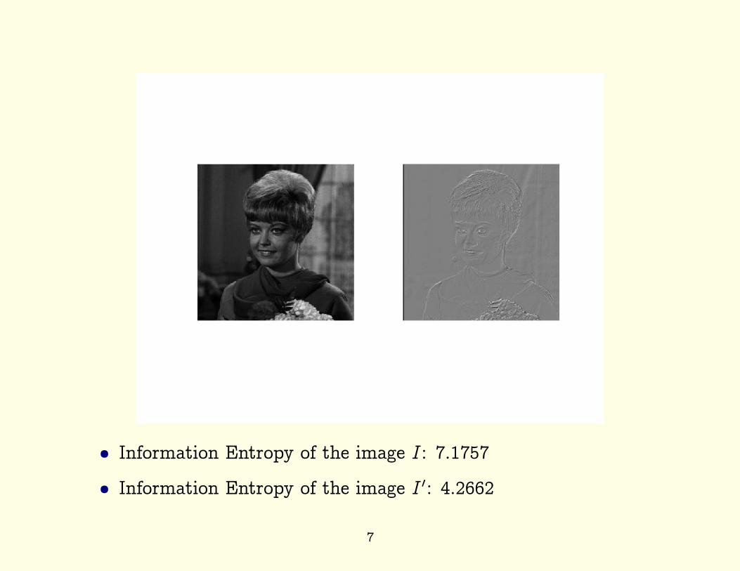
• Information Entropy of the image I: 7.1757
• Information Entropy of the image I ′: 4.2662
7
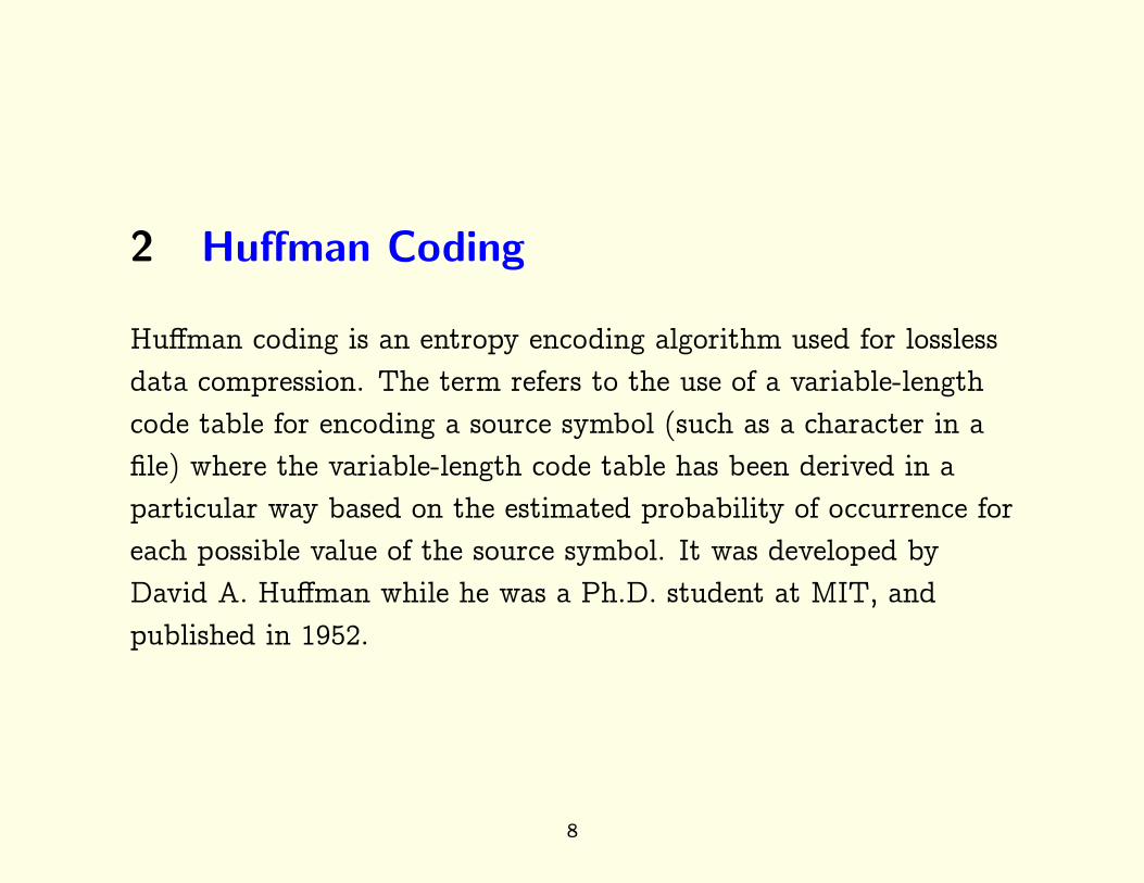
2 Huffman Coding
Huffman coding is an entropy encoding algorithm used for lossless
data compression. The term refers to the use of a variable-length
code table for encoding a source symbol (such as a character in a
file) where the variable-length code table has been derived in a
particular way based on the estimated probability of occurrence for
each possible value of the source symbol. It was developed by
David A. Huffman while he was a Ph.D. student at MIT, and
published in 1952.
8
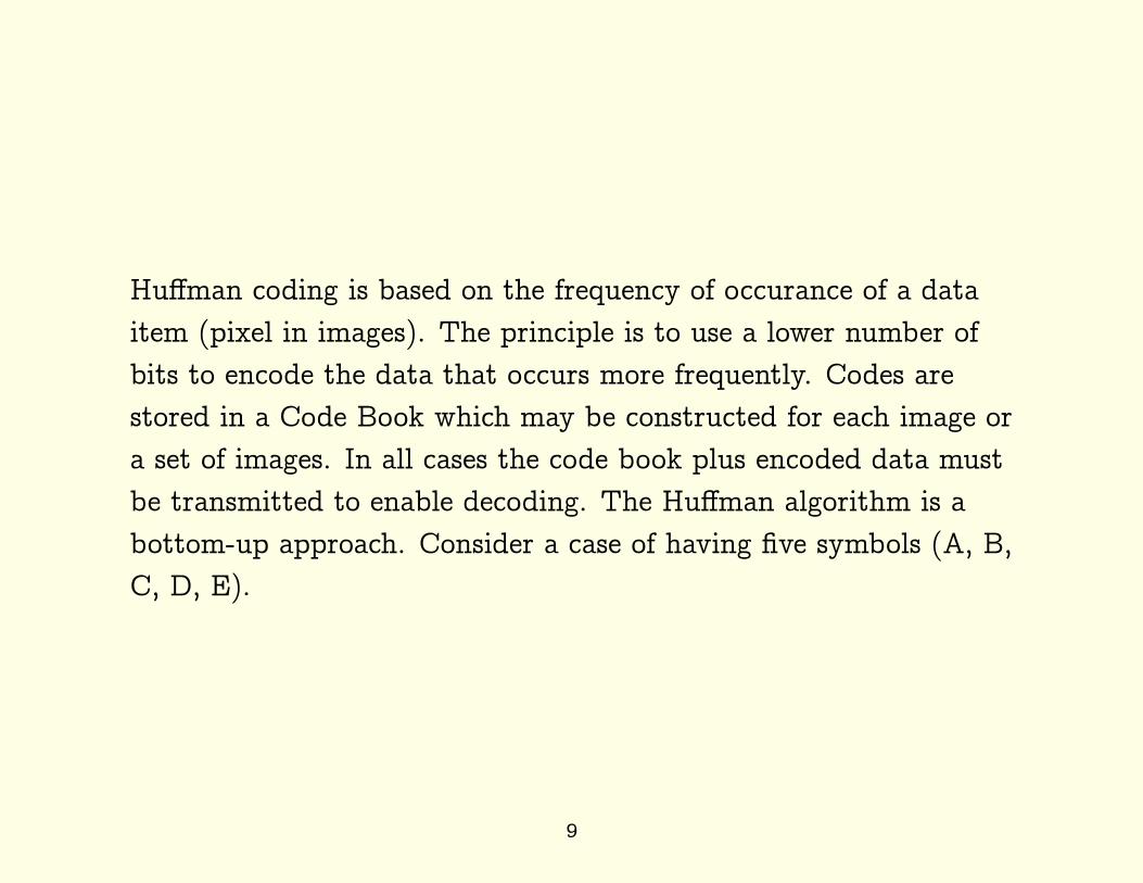
Huffman coding is based on the frequency of occurance of a data
item (pixel in images). The principle is to use a lower number of
bits to encode the data that occurs more frequently. Codes are
stored in a Code Book which may be constructed for each image or
a set of images. In all cases the code book plus encoded data must
be transmitted to enable decoding. The Huffman algorithm is a
bottom-up approach. Consider a case of having five symbols (A, B,
C, D, E).
9

Symbol Count Probability Entropy
A 15 0.3846 1.3785
B 7 0.1795 2.4780
C 6 0.1538 2.7004
D 6 0.1538 2.7004
E 5 0.1282 2.9635
Total 39 1.0000 2.1858 (average)
From this table, the theoretical total information is
2.1858× 39 = 85.2467 bits. If we use a fixed length code of 3 bits,
the total would be 4× 39 = 156 bits. The procedure of the
Huffman coding is as follows:
10

1. From the table, pick two nodes (symbols) having the lowest
frequencies or probabilities. Assign ’1’ to the one with the
lowest, then ’0’ to the second lowest. Or, simply assign ’1’ to
one of the two, and ’0’ to the other. Create a parent node of
these two symbols combined, ’DE’ for this case.
Symbol Count Probability Code
A 15 0.3846 -
B 7 0.1795 -
C 6 0.1538 -
D 6 0.1538 0
E 5 0.1282 1
11
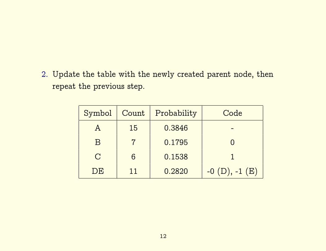
2. Update the table with the newly created parent node, then
repeat the previous step.
Symbol Count Probability Code
A 15 0.3846 -
B 7 0.1795 0
C 6 0.1538 1
DE 11 0.2820 -0 (D), -1 (E)
12
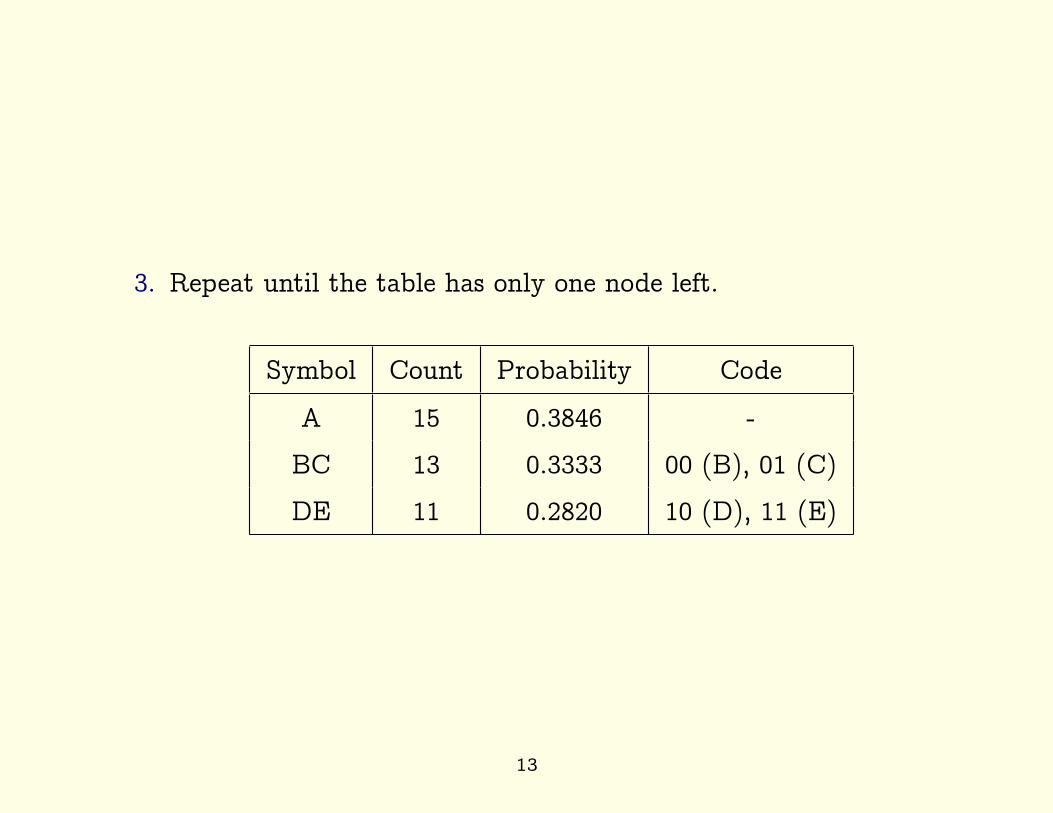
3. Repeat until the table has only one node left.
Symbol Count Probability Code
A 15 0.3846 -
BC 13 0.3333 00 (B), 01 (C)
DE 11 0.2820 10 (D), 11 (E)
13
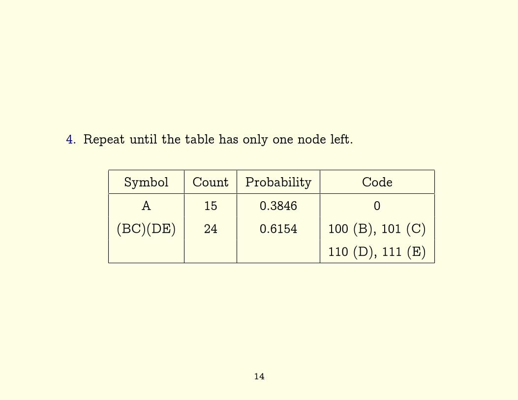
4. Repeat until the table has only one node left.
Symbol Count Probability Code
A 15 0.3846 0
(BC)(DE) 24 0.6154 100 (B), 101 (C)
110 (D), 111 (E)
14

15

Symbol Count Probability Entropy Code Subtotal
A 15 0.3846 1.3785 0 15
B 7 0.1795 2.4780 100 21
C 6 0.1538 2.7004 101 18
D 6 0.1538 2.7004 110 18
E 5 0.1282 2.9635 111 15
Total 39 1.0000 2.1858 (avg) 87
Compare this with the theoretical total information of
2.1858× 39 = 85.2467 bits.
16
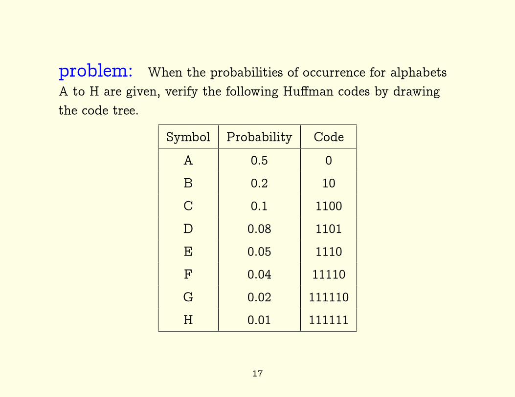
problem: When the probabilities of occurrence for alphabets
A to H are given, verify the following Huffman codes by drawing
the code tree.
Symbol Probability Code
A 0.5 0
B 0.2 10
C 0.1 1100
D 0.08 1101
E 0.05 1110
F 0.04 11110
G 0.02 111110
H 0.01 111111
17

3 JPEG Image Compression
A joint ISO/CCITT committee known as JPEG (Joint
Photographic Experts Group) has established the international
compression standard for continuoustone still images, both
grayscale and color, early in 1990’s. JPEG now supports four
modes of operation, sequential encoding, progressive encoding,
lossless encoding, hierarchical encoding. The most fundamental
sequential encoding that encodes a picture in a single left-to-right,
top-to-bottom scan, is discussed here. This is a lossy compression.
18

The encoder consists of 3 major components, (1) Forward DCT
(Discrete Cosine Transform, (2) Quantizer based on the
quantization table, and (3) Entropy Encoder that employs Huffman
coding and Run-Length coding. These are applied to each of three
components in the YUV (YCbCr) color space, sequentially.
The paper, Gregory K. Wallace, “The JPEG Still Picture
Compression Standard”, is a good reference available at
http://man.lupaworld.com/content/other/jpg.pdf
19

§1. Forward 8×8 DCT
An image is divided into a stream of 8× 8 blocks of gray scale
image samples. The image is scanned left-to-right, top-to-bottom.
Source image samples grouped in 8× 8 blocks are shifted from
unsigned integers [0, 2p − 1] to signed integers [−2p−1, 2p−1 − 1].
Each block of 8× 8 pixels is then transformed by the forward DCT
into the spectral domain. The forward DCT (FDCT) is given by
F (u, v) =1
4C(u)C(v)
7∑
x=0
7∑
y=0
f(x, y) cos(2x+ 1)uπ
16cos
(2y + 1)vπ
16
C(u), C(v) =
1√2
for u, v = 0
1 otherwise
20

clear all; close all;
I=imread(’lenna-y.jpg’);
imshow(I); hold on;
[x0,y0]=ginput(1);
x0=fix(x0); y0=fix(y0);
x=x0; y=y0;
x=[x-1,x+8,x+8,x-1,x-1]
y=[y-1,y-1,y+8,y+8,y-1]
plot(x,y,’-r’);
I88=double(I(x0:x0+7,y0:y0+7))-128
DCT88=fix(dct2(I88))
% FUJIFILM - FinePix F40fd ()
A=[6 5 6 6 7 10 20 29
4 5 5 7 9 14 26 37
4 6 6 9 15 22 31 38
6 8 10 12 22 26 35 39
10 10 16 20 27 32 41 45
16 23 23 35 44 42 48 40
20 24 28 32 41 45 48 41
24 22 22 25 31 37 40 40]
DQ=fix(DCT88./A)
21

An area of DCT block set in the eye. Numerical values are sampled
from this area.
22
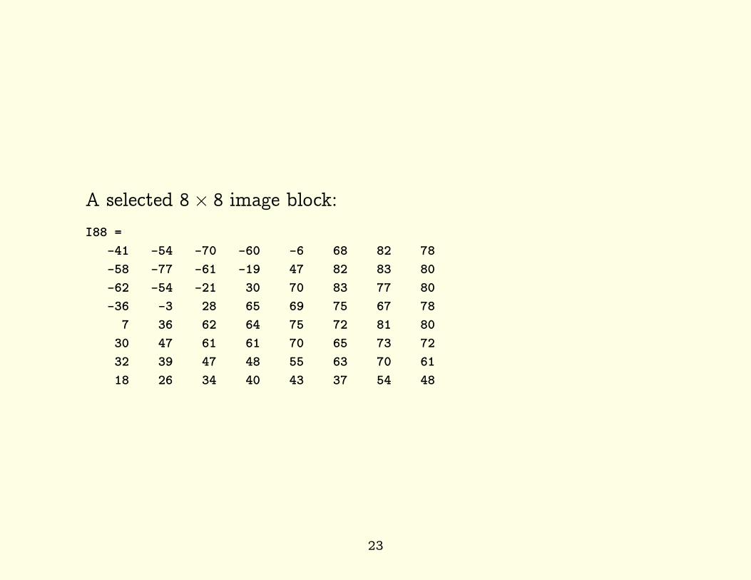
A selected 8× 8 image block:
I88 =
-41 -54 -70 -60 -6 68 82 78
-58 -77 -61 -19 47 82 83 80
-62 -54 -21 30 70 83 77 80
-36 -3 28 65 69 75 67 78
7 36 62 64 75 72 81 80
30 47 61 61 70 65 73 72
32 39 47 48 55 63 70 61
18 26 34 40 43 37 54 48
23

The result of forward DCT:
DCT88 =
286 -263 -35 20 -6 -3 0 3
-133 -164 18 52 3 -4 11 -7
-98 -17 66 41 -8 5 0 1
28 31 46 4 -20 -2 1 3
-7 21 14 -17 -11 0 -2 -4
0 7 4 -4 -6 0 1 -10
-4 4 0 -5 0 -1 -2 0
5 -3 4 2 -5 0 0 3
24

A quantization matrix (FUJIFILM - FinePix F40fd):
A =
6 5 6 6 7 10 20 29
4 5 5 7 9 14 26 37
4 6 6 9 15 22 31 38
6 8 10 12 22 26 35 39
10 10 16 20 27 32 41 45
16 23 23 35 44 42 48 40
20 24 28 32 41 45 48 41
24 22 22 25 31 37 40 40
25

The DCT matrix after quantizxation:
DQ =
47 -52 -5 3 0 0 0 0
-33 -32 3 7 0 0 0 0
-24 -2 11 4 0 0 0 0
4 3 4 0 0 0 0 0
0 2 0 0 0 0 0 0
0 0 0 0 0 0 0 0
0 0 0 0 0 0 0 0
0 0 0 0 0 0 0 0
26

4 Application of DCT to 8× 8 bolcks
DCT, Quantization, DC-component
The detailed procedure of JPEG encoding takes the following steps:
1. Subdivide a given picture into blocks of a 8 × 8 pixel area.
Then, process the blcoks sequentially from left-to-right then
top-to-bottom.
2. Convert pixel values of a block from the unsigned integer
[0, 2N − 1] to signed integer [−2N−1,+2N−1 − 1].
3. Apply 2D DCT to the block. For a 8 bit gray scale image
[0, 255], the values of 2D DCT transform are in the range of
−2048 ≤ I(i, j) ≤ 2048, 12 bits. The double summation makes
the possible largest value be 255 (8 bits) times 64, 8 × 8, (6
bits). The constant 14 divides the result by 4 or (2 bits). Thus,
27

the DCT values are 12 bits.
4. Divide each of the 8× 8 DCT elements by the corresponding
value in the quantization table.
5. Repeating these steps until all blocks are processed.
The encoding part of JPEG compression without Huffman and
Run-length coding looks like the following:
I=imread(’lenna-y.jpg’);
imshow(I);
Img=double(I);
% FUJIFILM - FinePix F40fd ()
A=[6 5 6 6 7 10 20 29
4 5 5 7 9 14 26 37
4 6 6 9 15 22 31 38
6 8 10 12 22 26 35 39
10 10 16 20 27 32 41 45
16 23 23 35 44 42 48 40
20 24 28 32 41 45 48 41
24 22 22 25 31 37 40 40]
28
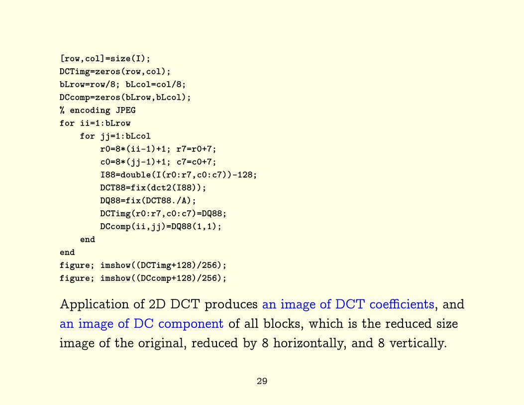
[row,col]=size(I);
DCTimg=zeros(row,col);
bLrow=row/8; bLcol=col/8;
DCcomp=zeros(bLrow,bLcol);
% encoding JPEG
for ii=1:bLrow
for jj=1:bLcol
r0=8*(ii-1)+1; r7=r0+7;
c0=8*(jj-1)+1; c7=c0+7;
I88=double(I(r0:r7,c0:c7))-128;
DCT88=fix(dct2(I88));
DQ88=fix(DCT88./A);
DCTimg(r0:r7,c0:c7)=DQ88;
DCcomp(ii,jj)=DQ88(1,1);
end
end
figure; imshow((DCTimg+128)/256);
figure; imshow((DCcomp+128)/256);
Application of 2D DCT produces an image of DCT coefficients, and
an image of DC component of all blocks, which is the reduced size
image of the original, reduced by 8 horizontally, and 8 vertically.
29

The original picture of Lena, and its quantized DCT image.
30
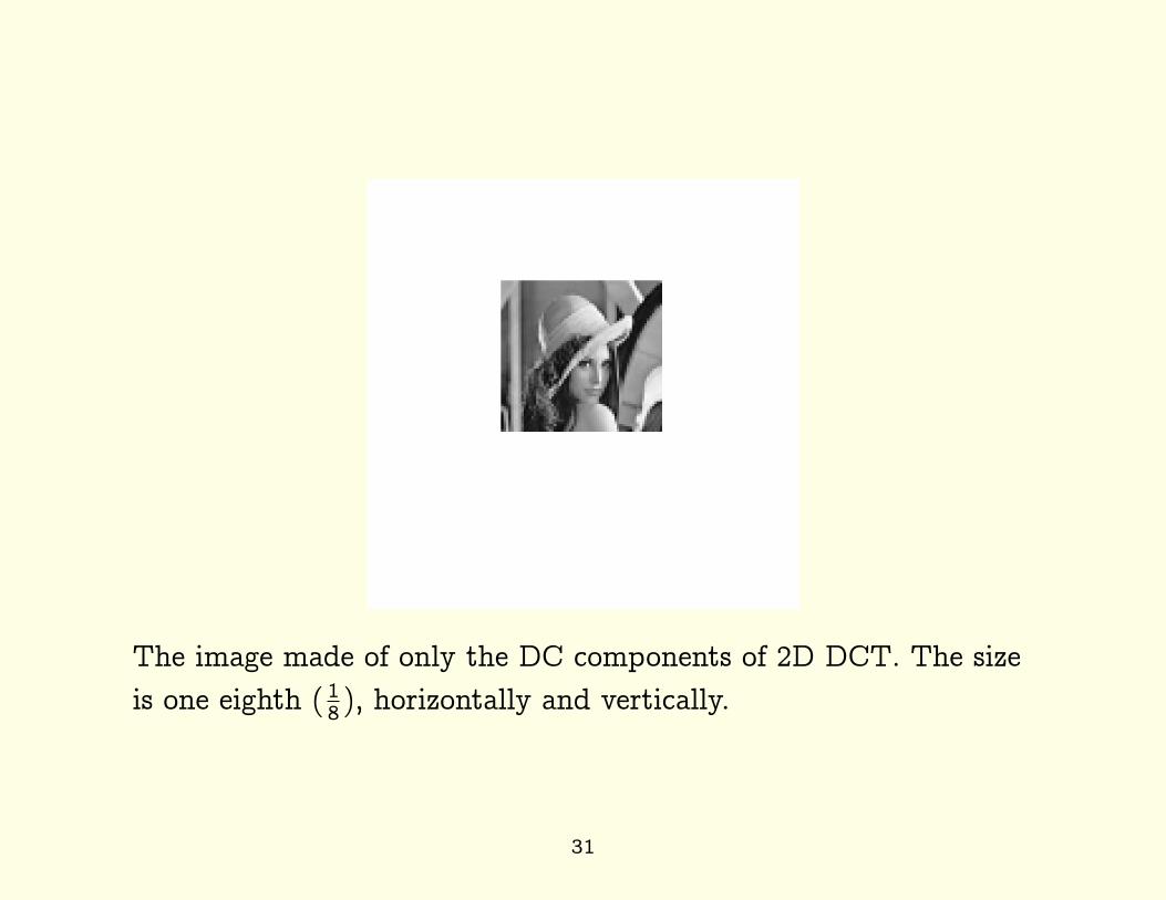
The image made of only the DC components of 2D DCT. The size
is one eighth ( 18 ), horizontally and vertically.
31
Inverse DCT to reconstruct a compressedJPEG image
In order to reconstruct the image from the quantized DCT
coefficients, actually the image of quantized DCT shown above, the
process of encoding with the 2D DCT was entirely reversed as
shown in the following MATLAB codes. The 2D DCT was replaced
by the 2D inverse DCT (iDCT2).
32

% decoding JPEG
RCNimg=zeros(row,col);
for ii=1:bLrow
for jj=1:bLcol
r0=8*(ii-1)+1; r7=r0+7;
c0=8*(jj-1)+1; c7=c0+7;
DQ88=DCTimg(r0:r7,c0:c7);
DCT88=DQ88.*A;
iDCT88=idct2(DCT88)+128;
RCNimg(r0:r7,c0:c7)=iDCT88;
end
end
figure; imshow(RCNimg/256);
33

The original picture of Lena, and its reconstructed image with the
inverse DCT and dequantization.
34
PSNR and Entropy Values
Image reconstruction from the DCT image, quantized DCT
coefficients to be exact, was successful in appearance. The peak
signal to noise ratio PSNR was measured for the reconstructed
image referenced to the original image. The value obtained was
37.8 dB. The peak value of 255 was used. The mean squared error
MSE was 10.78, giving an average error in magnitude be around
3.28, compared with the maximum pixel value of 255. The
information entropy was calculated for the original and the
reconstructed. They are very close, 7.4217 vs. 7.4080. The entropy
of the DCT image was only 1.0266, which means that this image
can be compressed down to about 1 bit per pixel.
35
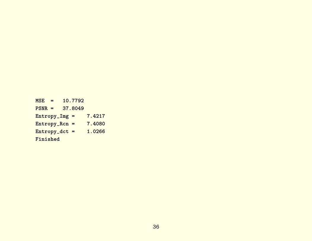
MSE = 10.7792
PSNR = 37.8049
Entropy_Img = 7.4217
Entropy_Rcn = 7.4080
Entropy_dct = 1.0266
Finished
36

The histogram of the original picture of Lena, and the histogram of
the DCT image.
37

MATLAB program to test JPEG encoding anddecoding
clear all; close all;
I=imread(’lenna-y.jpg’);
imshow(I);
Img=double(I);
% FUJIFILM - FinePix F40fd ()
A=[6 5 6 6 7 10 20 29
4 5 5 7 9 14 26 37
4 6 6 9 15 22 31 38
6 8 10 12 22 26 35 39
10 10 16 20 27 32 41 45
16 23 23 35 44 42 48 40
20 24 28 32 41 45 48 41
24 22 22 25 31 37 40 40]
[row,col]=size(I);
DCTimg=zeros(row,col);
bLrow=row/8; bLcol=col/8;
DCcomp=zeros(bLrow,bLcol);
% encoding JPEG
for ii=1:bLrow
38

for jj=1:bLcol
r0=8*(ii-1)+1; r7=r0+7;
c0=8*(jj-1)+1; c7=c0+7;
I88=double(I(r0:r7,c0:c7))-128;
DCT88=fix(dct2(I88));
DQ88=fix(DCT88./A);
DCTimg(r0:r7,c0:c7)=DQ88;
DCcomp(ii,jj)=DQ88(1,1);
end
end
figure; imshow((DCTimg+128)/256);
figure; imshow((DCcomp+128)/256);
% decoding JPEG
RCNimg=zeros(row,col);
for ii=1:bLrow
for jj=1:bLcol
r0=8*(ii-1)+1; r7=r0+7;
c0=8*(jj-1)+1; c7=c0+7;
DQ88=DCTimg(r0:r7,c0:c7);
DCT88=DQ88.*A;
iDCT88=idct2(DCT88)+128;
RCNimg(r0:r7,c0:c7)=iDCT88;
end
end
39

figure; imshow(RCNimg/256);
% Calculate PSNR
SSE=0;
for i=1:row
for j=1:col
SSE=SSE+(Img(i,j)-RCNimg(i,j))^2;
end
end
MSE=SSE/(row*col)
PSNR=10*log10(255^2/MSE)
Entropy_Img=entropy(Img/256)
Entropy_Rcn=entropy(RCNimg/256)
Entropy_dct=entropy((DCTimg+128)/256)
figure;
subplot(121); imhist(Img/256);
subplot(122); imhist((DCTimg+128)/256);
disp(’Finished’);
40
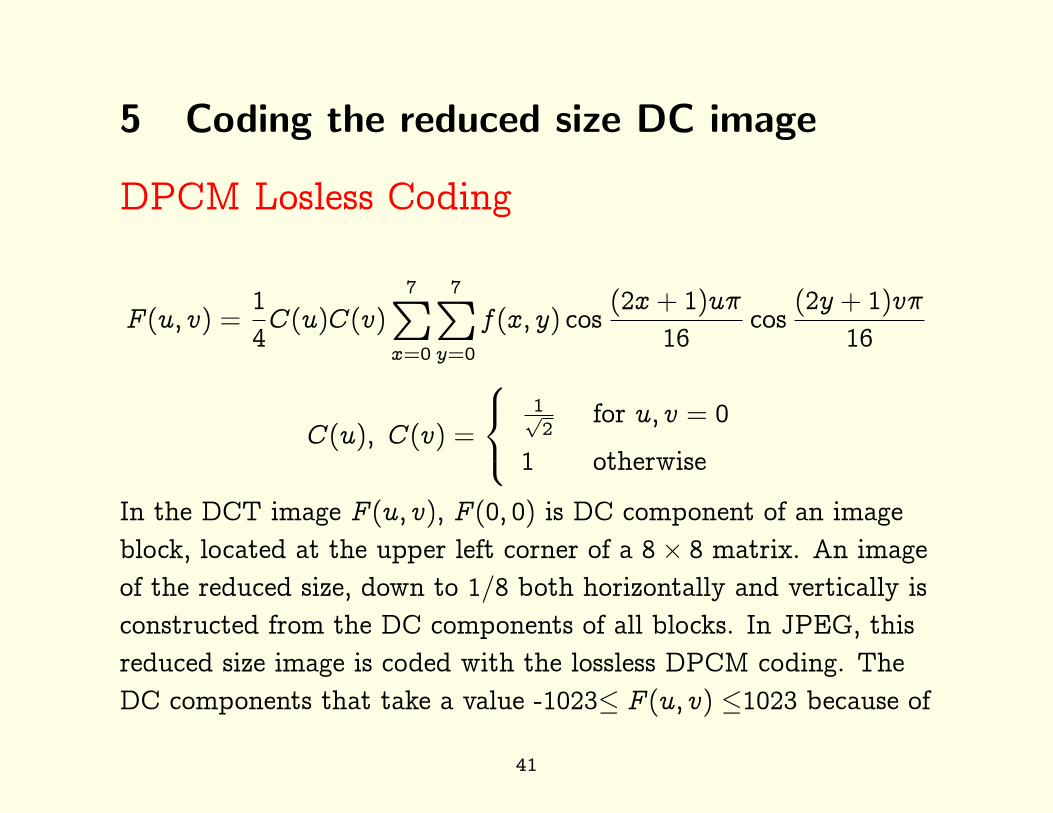
5 Coding the reduced size DC image
DPCM Losless Coding
F (u, v) =1
4C(u)C(v)
7∑
x=0
7∑
y=0
f(x, y) cos(2x+ 1)uπ
16cos
(2y + 1)vπ
16
C(u), C(v) =
1√2
for u, v = 0
1 otherwise
In the DCT image F (u, v), F (0, 0) is DC component of an image
block, located at the upper left corner of a 8× 8 matrix. An image
of the reduced size, down to 1/8 both horizontally and vertically is
constructed from the DC components of all blocks. In JPEG, this
reduced size image is coded with the lossless DPCM coding. The
DC components that take a value -1023≤ F (u, v) ≤1023 because of
41
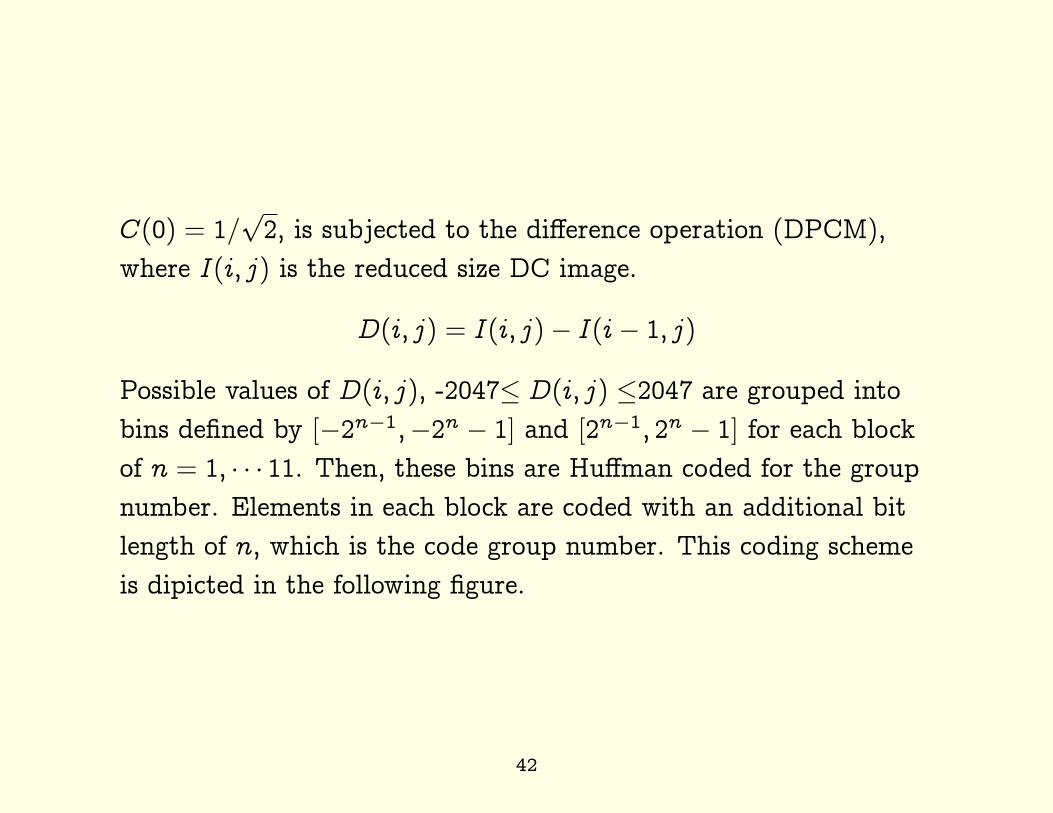
C(0) = 1/√
2, is subjected to the difference operation (DPCM),
where I(i, j) is the reduced size DC image.
D(i, j) = I(i, j)− I(i− 1, j)
Possible values of D(i, j), -2047≤ D(i, j) ≤2047 are grouped into
bins defined by [−2n−1,−2n − 1] and [2n−1, 2n − 1] for each block
of n = 1, · · · 11. Then, these bins are Huffman coded for the group
number. Elements in each block are coded with an additional bit
length of n, which is the code group number. This coding scheme
is dipicted in the following figure.
42

0(00)1(010)
2 (011)3(100)
4(101)5
67
89
1011
12
3
-7, -6, -5, -4 4, 5, 6, 78, 9, 10,11,12,13,14,15
(000,001,010,011) (100,101,110,111)
20471023
512255
12763
31
Group code
Difference code
43

Gr. Difference of DC values Group code Added bits
0 0 00 0
1 -1,1 010 1
2 -3,-2,2,3 011 2
3 -7..-4,4..7 100 3
4 -15...-8,8...15 101 4
5 -31...-16,16...31 110 5
6 -63...-32,32...63 1110 6
7 -127...-64,64...127 11110 7
8 -255...-128,128...255 111110 8
9 -511...-256,256...511 1111110 9
10 -1023...-512,512...1023 11111110 10
11 -2047...-1024,1024...2047 111111110 11
44

Examples:
• difference=-5, Group code (100) + Added code (011) =
(100011)
• difference=63, Group code (1110) + Added code (111111) =
(1110111111)
• difference=1, Group code (101) + Added code (1) = (1011)
• difference=0, Group code (00) + no Added code
45

6 Encoding DCT (AC) coefficients
Zigzag scanning
DCT coefficients of a block other than the DC components are
46

scanned in a zigzag fashion as shown in the figure above. The
zigzag scanning moves from lower frequencies to higher frequencies.
As the DCT tends to concentrate AC coefficients (components) in
the upper left area, the zigzag scan encounters more zeros as it goes
to higher frequencies. Therefore, JPEG uses Huffmann coding for
non-zero DCT coefficients, and Run-length coding to encode the
length of repeated zeros (of the DCT coefficinets) in order to
encode the DCT’s AC components.
Nonzero AC DCT coefficientsNonzero AC DCT coefficients, namely valid coefficients for Huffman
coding, are grouped into 10 groups. the same number of bits as the
group number are appended to the Huffman code for a group code.
47
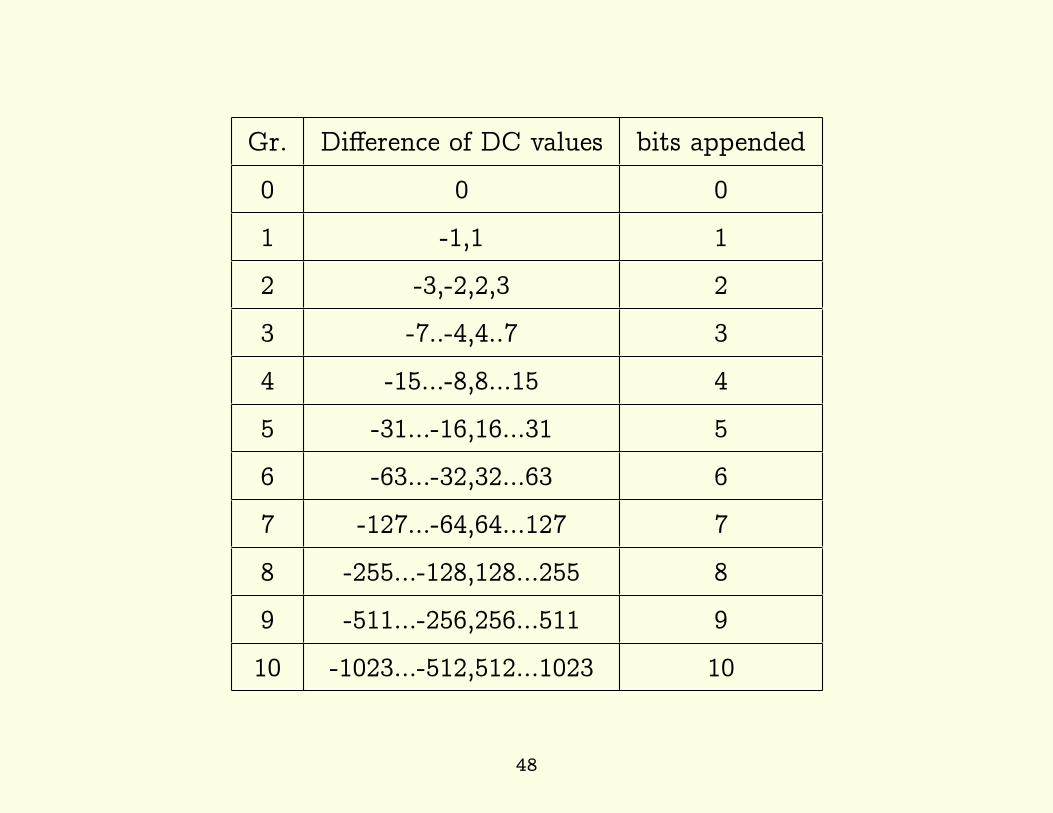
Gr. Difference of DC values bits appended
0 0 0
1 -1,1 1
2 -3,-2,2,3 2
3 -7..-4,4..7 3
4 -15...-8,8...15 4
5 -31...-16,16...31 5
6 -63...-32,32...63 6
7 -127...-64,64...127 7
8 -255...-128,128...255 8
9 -511...-256,256...511 9
10 -1023...-512,512...1023 10
48
Huffman coding for Run-length, GroupNumber combined
49

Gr. Group No. Huffman Code
0 EOB 1010
0 1 00
0 2 01
0 3 100
0 4 1011
0 5 11010
0 6 1111000
0 7 11111000
0 8 1111110110
0 9 111111110000010
0 10 111111110000011
1 1 1100
1 2 11011
1 3 1111001
1 4 111110110...
......
50
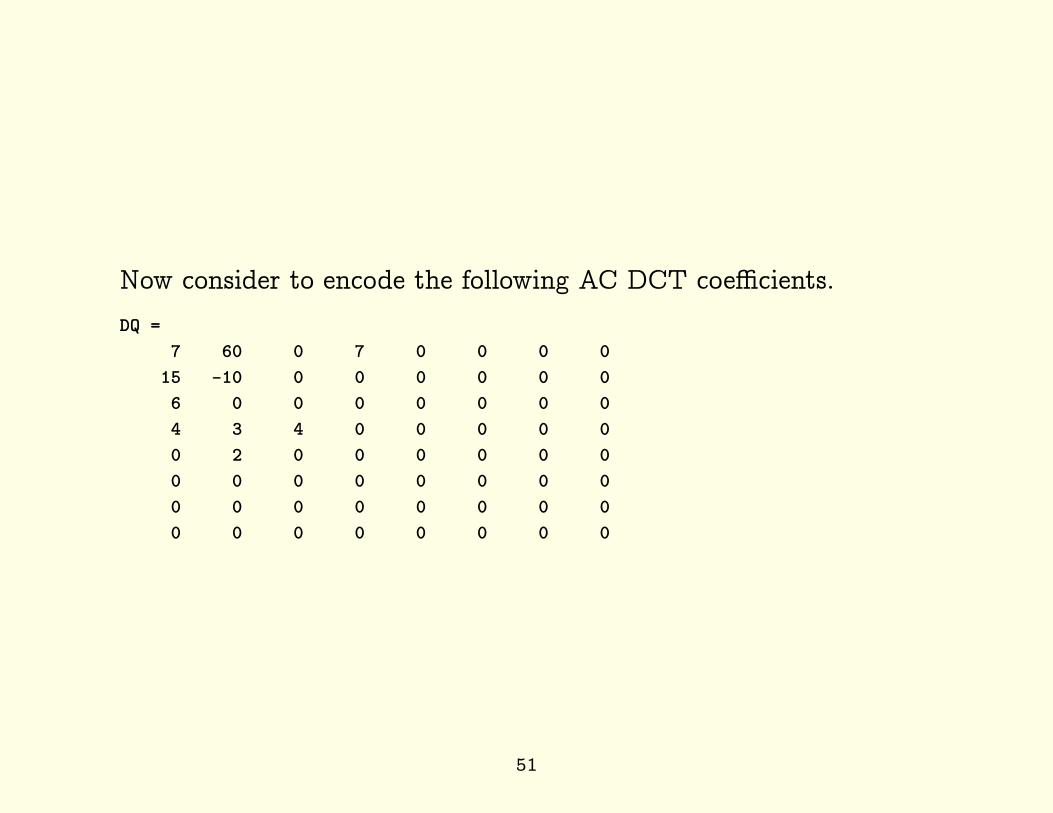
Now consider to encode the following AC DCT coefficients.
DQ =
7 60 0 7 0 0 0 0
15 -10 0 0 0 0 0 0
6 0 0 0 0 0 0 0
4 3 4 0 0 0 0 0
0 2 0 0 0 0 0 0
0 0 0 0 0 0 0 0
0 0 0 0 0 0 0 0
0 0 0 0 0 0 0 0
51
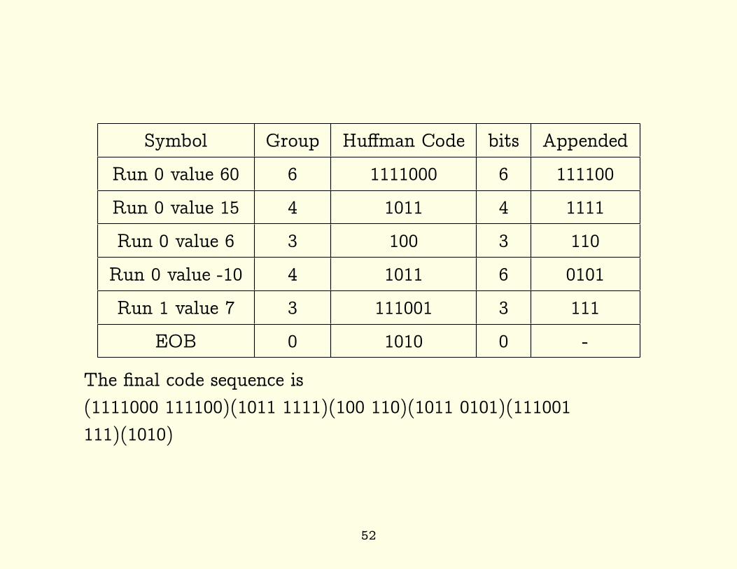
Symbol Group Huffman Code bits Appended
Run 0 value 60 6 1111000 6 111100
Run 0 value 15 4 1011 4 1111
Run 0 value 6 3 100 3 110
Run 0 value -10 4 1011 6 0101
Run 1 value 7 3 111001 3 111
EOB 0 1010 0 -
The final code sequence is
(1111000 111100)(1011 1111)(100 110)(1011 0101)(111001
111)(1010)
52
Chroma Subsampling
Color images are transformed from RGB to YUV in JPEG. Luma
component Y, and two chroma components U (Cb) and V (Cr) are
independently quantized then entropy coded. However, chroma has
less amount of informatio compared with luma. In JPEG, chroma
subsampling can be specified. Chroma subsampling notation is
shown in the figure below. Typically, one of 4:4:4, 4:2:2, or 4:2:0 is
used.
53
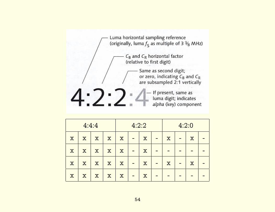
4:4:4 4:2:2 4:2:0
x x x x x - x - x - x -
x x x x x - x - - - - -
x x x x x - x - x - x -
x x x x x - x - - - - -
54
7 Assignment JPEG
Free, portable C code for JPEG compression is available from the
Independent JPEG Group. Source code, documentation, and test
files are included. Version 6b is available from
ftp.uu.net:/graphics/jpeg/jpegsrc.v6b.tar.gz. If you are on a PC
you may prefer ZIP archive format jpegsr6b.zip, which you can find
at http://www.sac.sk/files.php?d=5&l=J This assignment is to
compile this JPEG source code on either PC or Linux platform
then study jpeg files produced by this software with various control
parameters.
This free portable C code was tested with djgpp on Windows XP.
Djgpp is a complete 32-bit C/C++ development system for Intel
80386 (and higher) PCs running DOS. If you are not familiar with
Linux (Unix based PC operating system), you are advised to use
55
djgpp. Note that this source code jpegsr6b.zip provides Makefile
and config.h for djgpp, but not specifically for Linux.
• The coding part of the compiled program cjpeg.exe has a
command line switch -quality N which scales the quantization
tables to adjust image qaulity. Quality is 0 (worst) to 100
(best); default is 75. For an image of your choice in ppm, bmp,
gif, run cjpeg.exe with different setting of -quality N to obtain
an output image of that specified quality. Calculate first the
entropy of the input image to compare the degree of
compression achieved for varied -quality N. Try N=100, N=75,
N=50, N=25 and N=10. Measure the achieved entropy by
dividing the total number of bits of the jpeg file by the image
size. Also calculate MSE and PSNR of each image generated.
Discuss how -quality N affects compression, and image quality.
• The ”wizard” switches are intended for experimentation with
56

JPEG. These switches are documented in the file wizard.doc.
One of the wizard switches is -qtables file. You can specify
the quantization tables given in the specified text file to use it
instead of default file. Quantization tables used in digital
cameras are found at
http://www.impulseadventure.com/photo/jpeg-
quantization.html. Try the Quantization Table for FUJIFILM -
FinePix F40fd () to encode your image. Discuss how this
quantization table affects compression, and image quality.
• By default, cjpeg uses 2:1 horizontal and vertical
downsampling when compressing YCbCr data. Other chroma
subsampling can be experimented by -sample HxV[,...]. Try
4:4:4, 4:2:2 and 4:2:0. Discuss how this switch for setting
subsampling factor affects compression, and image quality.
57