EFFICIENCY IN AGRICULTURAL PRODUCTION OF BIODIVERSITY:

ORGANIC VS. CONVENTIONAL PRACTICES

Timo Sipiläinen*, Per-Olov Marklund# and Anni Huhtala*

*MTT Agrifood Research Finland, Luutnantintie 13, 00410 Helsinki, Finland #Department of Economics, University of Umeå, Sweden

Contact: Anni Huhtala, anni.huhtala@mtt.fi, phone: +358-9-56080

Paper prepared for presentation at the 107th EAAE Seminar "Modeling of Agricultural and Rural Development Policies". Sevilla, Spain, January 29th -February 1st, 2008 Copyright 2007 by Timo Sipiläinen, Per-Olov Marklund and Anni Huhtala. All rights reserved. Readers may make verbatim copies of this document for non-commercial purposes by any means, provided that this copyright notice appears on all such copies.

Abstract

Promotion of environmental sustainable farming practices is an important policy goal for the whole

agricultural sector. However, when the efficiency of production is measured in practice,

enhancement of environmental quality such as biodiversity and other environmental amenities does

not seem to be recognized as a positive output produced by agriculture. Here, we include crop

diversity index as an indicator of environmental output in a comparison of efficiency of

conventional and organic crop farms. Non-parametric technical efficiency scores are estimated

applying data envelopment analysis on a sample of Finnish crop farms for 1994 – 2002. The results

show that in a pooled data set conventional crop farms are more technically efficient than organic

farms when only crop output is considered. When taking crop diversity into account the difference

between production techniques vanishes. In separate comparisons of conventional and organic

farms, the average efficiencies of the two groups do not differ statistically significantly. Thus, the

assumptions on the technology and reference sets are crucial with respect to the results of the

comparison. This has important implications for policy evaluations when alternative farming

technologies are compared.

JEL Classification:

Keywords: crop diversity, Shannon index, DEA, technical efficiency

1

1. Introduction

Agriculture is inherently multifunctional producing both food and fiber but also a wide range of

other outputs and services. That is why the concept of multifunctionality has been adopted when

reforming the European common agricultural policy to meet the demands of consumers with

heterogeneous preferences. The challenge is how to translate the diverse objectives into effective

policies. Increasing emphasis has been placed on the stewardship like payment schemes and social

type objectives when support for farmers cannot be justified only as an effort to secure food supply

(Dobbs and Pretty, 2004).

Biodiversity conservation on agricultural land is one of the objectives that has received a

considerable attention from policy makers when policies have been developed to pursue

environmental targets (see Wossink and van Wenum, 2003; van Wenum et al., 2004). As

agriculture has shaped the landscapes for centuries, much of the apparently “natural” biodiversity in

Europe is in fact a result of active farming practices. Evidently, agricultural production plays an

important role in conserving biodiversity, and promotion of environmental sustainable farming

practices is an overall goal for the whole sector independently of technology adopted. However, it

seems that enhancement of environmental quality, such as biodiversity, is not explicitly recognized

as a proper target, or a positive output when production efficiency is measured in practice. We

hypothesize that this ignorance may create biases in traditional efficiency scores, and incomplete

scores may discriminate environmentally benign technologies. This is an important issue to be taken

into account in comparison of conventional and organic farming technologies in agriculture.

Several studies have investigated the differences in technical efficiency of organic and conventional

farms. The results of Oude Lansink et al. (2002) indicate that the productivity of organic farms is

considerably lower than that of conventional farms. In particular, productivity of capital, but also

productivity of land and labor are low on organic farms. According to Ricci Maccarini and Zanoli

(2004), this may be related to problems of converting from conventional to organic farming.

Sipiläinen et al. (2005) show that technical efficiency decreases considerably when the conversion

to organic farming starts but that significant learning effects can be observed over time even though

the recovery of technical efficiency takes for a fairly long time. However, the previous studies only

have taken into account inputs and outputs that are included in a standard bookkeeping. They do not

take possible external effects - like nutrient leakages or landscape values - of different technologies

into account. Including these effects may have a significant effect on efficiency and productivity

2

measures. For example, crop rotation requirements suggest that organic farming may be

characterized by more diverse cropping systems than conventional farming.

The existing studies on environmental performance of organic and conventional farms provide

contradictory results on how well organic farming technology uses natural resources (Stoltze et al.,

2000; Oude Lansink et al., 2002). Hole et al. (2005) have analyzed extensive literature on

biodiversity and several biodiversity enhancing measures to investigate the superiority of organic

farming in the biodiversity conservation. Even though further research is required to assess the

performance of organic systems, they conclude that organic farming could play a significant role in

increasing biodiversity. However, no economic impacts were considered in their analysis.

Our contribution is to analyze efficiency in production within the frame of economic theory by

taking into account biodiversity as a good output produced on farms. The motivation is that if the

environmental goals are truly part of agricultural policies, the performance of policies implemented

should be possible to evaluate. In particular, it is necessary to have indicators for following up how

the policies implemented have become manifested in technology choices and corresponding

(environmental) benefits accrued. As the scarcity of resources is a point of departure for an

economic analysis we make explicit the trade-offs in production of market and non-market outputs.

It is these trade-offs that ultimately determine the costs of agri-environmental policies implemented.

The purpose of this paper is to estimate the performance of conventional and organic crop farms

and to evaluate the effect of the inclusion of biodiversity on performance measures. Our measure of

biodiversity, or more specifically, crop diversity is a farm level Shannon diversity index, which

captures both richness and evenness of cultivated crops on the farms. Thus, we rely in our analysis

on a landscape diversity indicator and do not consider for example genetic diversity. We evaluate

how efficient alternative farming practices are in using scarce resources in production of both crop

yield and crop diversity.

We compare how efficient production is when only conventional output (crop yield) and when also

environmental by-product (biodiversity) is taken into account. Moreover, we consider efficiency

scores when one of the outputs is held as a minimum constraint. Non-parametric technical

efficiency scores are estimated applying data envelopment analysis (DEA). The empirical analysis

is based on annual cross sections of Finnish crop farms participating in the bookkeeping system for

1994 – 2002. Since the number of organic farms is small we first rely on the assumption that both

3

conventional and organic farms face the same production frontier, although organic production can

be seen as a more restricted production technology1. In addition, we estimate efficiency scores for

organic and conventional technologies separately. In this separate estimation we apply so called

window analysis (Charnes et al., 1985) for organic farms. In that case we assume progressive

technical change in four year periods.

The results show that when only crop output is considered assuming that all farms face the same

production frontier, conventional crop farms are more technically efficient than organic farms.

When taking into account the effect of crop diversity on economic performance the difference

between the farming technologies vanishes. On average, efficiency scores are even higher on

organic than conventional farms. In separate comparisons of conventional and organic farms,

assuming different production frontiers the average efficiencies of the groups do not differ

significantly. This shows that the assumptions made about the technology and reference sets are

crucial with respect to the results of the comparison.

The paper is organized as follows. In Section 2 we introduce the crop diversity index applied in the

study and in section 3 we elaborate the production economic grounds of the study. Section 4

presents the empirical method and the next section the Finnish data. Section 6 includes empirical

results and the last section concludes.

2. Biodiversity - Crop diversity

Biodiversity (biological diversity) is defined as the variety of all forms of life and can be subdivided

into genetic diversity, species diversity, and ecological or ecosystem diversity (Biodiversity, 2005).

The concept is widely used, and a distinction can be made between functional – emphasizing the

perspective of ecosystem and evolutionary processes - and compositional – emphasizing in turn the

perspective of populations, species and other categories (Callicott et al., 1999). Biodiversity is also

often connected to the conservation of biological variation, the extent and future value of which are

largely unknown.

1 Organic farming as a method of production puts high emphasis on environmental protection. It avoids, or largely reduces, the use of synthetic chemical inputs like fertilizers, pesticides or additives. In the field of crop production fertilization with manure, growing legumes to bind nitrogen from the air, compost of vegetables of low soluble fertilizers, and preventive measures to control pests and diseases, are used. Also crop rotations, mechanical weed control and protection of beneficial organisms are important (Organic Farming in the EU: Facts and Figures, 2004). These restrictions most likely affect the performance of organic farms.

4

Two different schools of considering diversity have evolved in the literature, where different

species are given different weights. The ecological school weighs different species according their

relative abundance, whereas the economical school emphasizes that different species should be

given different weights in the diversity measure due to the attributes they possess (Baumgärtner,

2005). The attributes are what the society actually values and consumes. Here we choose to

incorporate an ecological measure of diversity into an economical production theory framework.

This approach is based on the idea that the ecological diversity is a good that the society values.

In agricultural systems, biodiversity may be produced as a positive by-product in addition to

marketable output such as cereals. Management practices may have various impacts on biodiversity

due to crop rotation, application of chemical inputs etc. The problem is that biodiversity is a

complex concept with several dimensions. Therefore, it is a challenge to choose proper measures or

indicators for biodiversity. The availability of data is a major limitation for the empirical analysis.

Here, we rely on a relatively simple measure of biodiversity, so called crop diversity index which

can be described as a landscape diversity measure. According to a classification of Callicott et al.

(1999) crop diversity index belongs to compositional measures of species diversity.

The species level of biodiversity is quantified in the number of species in a given area (richness)

and how evenly balanced the abundances of each species are (evenness) (Armsworth et al., 2004).

Note that the species level biodiversity is only one of the levels that can be used in analyzing the

biodiversity issue. For example, community level biodiversity describes the species interactions in

their natural habitats. The spatial scale is also important since richness increases with area. Usually

the choice is either an economically or an ecologically meaningful scale. We choose to study the

diversity of agricultural land use at the farm level, within an economical production theory

framework. At the farm level, we know the number of crops cultivated and the area under these

specific crops.

In this study, richness is measured by the number of cultivated crops like barley, grass silage,

potato, or fallow. Evenness refers to how uniformly the arable land area of the farm is distributed to

these different crops. Evenness and richness, describing diversity, can be quantified by Shannon

diversity index (SHDI) (Armsworth et al., 2004). It has its origin in the information theory

(Shannon 1948) and it has been applied in a number of environmental economic studies (e.g., Pacini

et al., 2003; Hietala-Koivu et al., 2004; Latacz-Lohman, 2004; Miettinen et al., 2004; Di Falco and

Perrings, 2005).

5

SHDI is calculated applying the following formula:

)ln(1

i

J

ii PPSHDI ×−= ∑

=

(1)

where J is the number of cultivated crops, Pi denotes the proportion of the area covered by a

specific crop and the natural logarithmn 2. The diversity index in equation (1) equals zero when

there is only one crop, indicating no diversity. The value increases with the number of cultivated

crops and when the cultivated areas under various crops become more even. The index reaches its

maximum when the crops are cultivated in equal shares, i.e., when Pi =1/J (McGarical and Marks

1995).

In this paper, the index is used to approximate the diversity produced by farms, and is therefore

modeled as a good output within the frames of production theory. Crop diversity has usually been

applied as a landscape indicator at the regional level. However, the use of crop diversity as a proxy

for biodiversity at the farm level can be motivated by the fact that the number of different habitats is

likely to increase with crop diversity. In conventional farming, a monoculture may be successful

whereas organic production technology sets higher requirements for crop rotation ruling out the

possibility of monoculture. Thus, organic farming technology is likely to produce higher crop

diversity. Numerous studies have also shown that crop rotations conserve soil fertility (Riedell et

al., 1998; Watson et al., 2002), improve nutrient and water use efficiency (Karlen et al., 1994) and

increase yield sustainability (Struik and Bonciarelli, 1997; see also Herzog et al., 2006).

3. Production Theory

3.1 Technology

To describe production technology formally, let and Mmyyy +ℜ∈= ),...,( 1 1( ,..., ) N

nx x x += ∈ℜ

}

be

vectors of outputs and inputs, respectively. Production technology can then be represented by the

output possibilities set

{ TyxyxP ∈= ),(|)( (2)

2 Shannon diversity index appears in the literature by names Shannon-Wiener (-Weiner or –Weaver) index. According to Keylock (2005) it belongs to the Hill family of indices (like Simpson diversity index) and is based on Bolzmann-Gibbs-Shannon entropic form. Sometimes the index is presented in the form of exp(SHDI). At the maximum the latter form provides the number of species for the uniform distribution (maximum entropy).

6

which describes all feasible output and input combinations of the producer. The technology is

denoted by T , and the condition is interpreted as can produce Tyx ∈),( x y . We assume that

is convex, closed, and bounded, i.e., compact, and that)(xP { }0)0( =P . The latter equality ensures

that inactivity is possible but there is no free lunch. Finally, outputs and inputs are assumed to be

freely disposable.

Input and output distance functions can be used to describe the technology when only input and

output quantities are known (Shephard, 1953; 1970). In contrast to the traditional scalar-valued

production function, distance functions allow multiple outputs (and multiple inputs). For any (x,y)

∈ R+M+N the output distance function Do(x,y) is such that

Do(x,y) = min {λ > 0: y/λ ∈ P(x)}. (3)

The output distance function calculates the largest expansion of y along the ray through y as far

from 0 as possible while staying in P(x), which means that y belongs to the producible output set if

and only if Do(x,y) ≤ 1. It is also obvious that the distance function takes the value one only if the

output vector belongs to the frontier of the corresponding input vector. Therefore, the output

distance function completely characterizes the technology, because it inherits its properties from

P(x).

The Farrell (1957) measure of output oriented technical efficiency is the reciprocal of the output

distance function, i.e. Fo(x,y) = (Do(x,y))-1. Thus

Fo(x,y) = max {µ: µy∈ P(x)}. (4)

Probably the most often used models of technical efficiency are variants of the Farrell type model3.

By duality output and input orientations have a convenient interpretation as an increase in revenue

and a reduction in costs, respectively. One desirable property of the Farrell type measure is that it is

invariant with respect to the units of measurement in inputs and outputs.

3 Chambers et al. (1998) have shown that the proportional distance function (the reciprocal of Farrell technical efficiency) is a special case of directional distance functions.

7

3.2 Modeling Biodiversity as a Good Output

To illustrate the measurement of technical efficiency, we assume first that a farm is producing only

one good output, crop (Figure 1a). At the output level b (on the vertical axis) and input level a (on

the horizontal axis), the technical output efficiency of the farm depends on the choice of reference

set. If the reference set is technology 1 the efficiency is 0b/0c, but if it is technology 2 the efficiency

is lower, 0b/0d. In this context, technology 2 is more productive than technology 1, which may be

constrained by restrictions on the use of inputs or crop rotation requirements (as is the case for

organic farming technology).

Figure 1a and b. An illustration of technical output efficiency in one (crop) and two output (crop

and crop diversity) cases.

In Figure 1a we only consider production of crops that can be sold on the market. However,

agricultural production provides also other, non-market outputs. This is illustrated in Figure 1b

where we have two outputs: crop output and non-market crop diversity. The transformation curves

Common frontier

Technology 1

0

Crop

g f

e

j

i

h

Technology 2

Crop diversity

d

c

b

a

Technology 1

Technology 2

a Crop

0 Input

b

8

show how much of the crop output has to be sacrificed to increase crop diversity, given inputs.

Technologies 1 and 2 (organic vs. conventional) which allow for different production possibiliti

a given input level are illustrated by two separate transformation curves (or outer boundaries of

producible output sets). Technical efficiencies are derived from the radial distances from the

frontier. For example, a technical efficiency score for point e with respect to technology 1 (0e

different compared to technical efficiency with respect to technology 2 (0f/0g). In our illustration in

Figure 1b, producible output sets of the two technologies cross

es at

/0g) is

e

to

. Empirical Method

odels

y efficient if it lies on the boundary of the output possibility set,

envel

he DEA models applied in this study are output oriented assuming that P(x) satisfies convexity. If

s

EA models are fairly simple linear programming (LP) models which have to be solved for each

l

4. Therefore, if we use a common,

joint reference frontier without separating two underlying technologies, it is defined by the units

representing different technologies. In the high crop output – low crop diversity dimension the

frontier is defined by the units applying technology 2 but in the opposite case it is defined by th

units using technology 1. Figure 1b shows that the assumption of whether all farms having access

the same technology, or of whether organic and conventional farms not having access to the same

technology, may be crucial in the measurement of efficiency.

4

4.1 Data Envelopment M

The firm is said to be technicall

)(xP . There are several possibilities to define the boundary, often referred as the frontier. Data

opment analysis (DEA) is a non-parametric method that provides a piecewise linear, either

convex or non-convex envelopment for the observations. It has been developed for evaluating the

performance of multi-input multi-output production (see Debreu, 1951; Farrell, 1957 and

Koopmans, 1951; Charnes et al., 1978).

T

technical efficiency obtains its maximal value (one), the production is efficient, and it is not

possible to increase output (given inputs) in comparison to the reference units. If production i

technically output inefficient, output can be increased using given inputs.

D

decision making unit (farm) separately. In the case of variable returns to scale, we define the mode

with outputs, ym, and inputs, xn, when k decision making units form the reference set and each of

them, k’, is in turn compared to the reference set. In our notation below, ( , )oF VRS S or φ denotes

4 It is of course possible that one of the technologies dominates at all output combinations.

9

technical output efficiency under variable returns to scale (V) and strong disposability (S)

assumptions. The efficiency measure is the reciprocal of output distance function, ( ( ,oD x y 1))−

the LP pro em.

. . , 1,..., ,

, 1,... ,

1,

0, 1,..., .

Kt tk m k km

kK

t tk kn k n

kK

kk

k

s t y z y m M

z x x n N

z

z k K

(Färe et al., 1994). The superscript t in Equation (5) refers to the annual solution of bl1( , ) ( ( , )) maxt

o oF VRS S D x y

'1

'1

1

φ

φ=

=

=

≤ =

≤ =

=

≥ =

∑

∑

∑

(5)

he DEA model of variable returns to scale is obtained by a constraint for intensity

lution such that

nd to be

le is

we are only interested in technical efficiency of crop production, disregarding crop diversity, we

at

−= =

T

variables 1kz =∑ , which restricts the scaling of units in the search for an optimal so

the sum of weights of the observations has to equal to one. When the intensity variables z are not

constrained, the scaling of reference units up and down is unlimited, which coincide with constant

returns to scale (CRS). The CRS assumption implies that the efficiency ranking of units is

independent of the choice of orientation, be it input or output. In agriculture, larger farms te

more technically efficient than smaller ones when assessed by the CRS DEA model (e.g.,

Sipiläinen, 2003). The possible heterogeneity in size, or indication on the economies of sca

partially removed when VRS models are applied. This also supports the VRS type model for our

application as the average sizes of farms in alternative production technologies differ.

If

may apply the model with only one traditional crop output. We may, however, easily extend the

analysis taking into account other outputs. If we assume that crop diversity is a desirable output th

farms also produce we may solve the LP problem with two outputs. The very nature of the DEA

models is that after adding other outputs the number of efficient decision making units increases.5

This property coincides with the problem of omitted outputs since in that case we may

underestimate the true technical efficiency of a decision making unit.

5 Coelli et al., (1998) writes: ”The addition of an extra input or output in a DEA model cannot result in a reduction in the technical efficiency scores” (p. 181).

10

The traditional two output DEA model assumes that the efficiency score is calculated as a

possibility for an equi-proportional increase in outputs, given inputs and reference units. Thus, we

in principle assume that socially optimal proportions of these outputs are already produced but our

target is to produce more both of them. This is a critical assumption when we take into account non-

market outputs which do not have a market price. We may also think that the target of the society

would be to increase either crop diversity given inputs and traditional output or to increase

traditional output given inputs and crop diversity. This would be interpreted as if a socially optimal

level of one of the outputs was already produced but the purpose was to evaluate the possibilities to

increase the other output. To assess these options, we introduce in the LP model a slightly different

set of constraints. In particular, we assume that only the traditional output is adjusted but the crop

diversity is treated as an ordinary constraint indicating that crop diversity of the feasible solution

should be at least as large as in our decision making unit. Technical efficiency is thus only

measured in relation to traditional output. This is similar to technical sub-vector efficiency

introduced by Färe et al. (1994), and applied to variable inputs by Oude Lansink et al. (2002).

Traditional technical efficiency and sub-vector efficiencies are illustrated in Figure 2. The output set

includes both crop output and crop diversity. Traditional Farrell type technical output efficiency is

measured as a proportional expansion of outputs along the solid line from point A to the frontier.

The crop sub-vector efficiency specified in Equation (6) below is described as an increase of crop

output along the vertical broken line from point A to the frontier, and crop diversity sub-vector

efficiency is defined as an expansion of crop diversity output along the horizontal dotted line from

point A to the frontier.

Crop

Crop subvector efficiency

Figure 2. An illustration of traditional and sub-vector technical efficiencies.

Radial technical efficiency

A

Crop diversity subvector efficiency

Crop diversity

11

A formal presentation of the crop sub-vector efficiency when m=1 denotes crop output and m=2

crop diversity is the following6:

1

1 ' 11

2 ' 21

'1

1

( , , ) ( ( , )) max

. .

, 1,... ,

1,

0, 1,..., .

to o

Kt tk k k

k

Kt t

k k kk

Kt t

k kn k nk

K

kk

k

F VRS S sub D x y

s t y z y

y z y

z x x n N

z

z k K

φ

φ

−

=

=

=

=

= =

≤

≤

≤ =

=

≥ =

∑

∑

∑

∑

(6)

We still have to choose the reference sets for the efficiency analysis. When solving an optimization

problem applying an annually pooled data set we actually assume that the farms have access to each

others’ technology independently of their actual farming technology (conventional or organic). In

other words, efficient units and their linear combinations may consist of organic and/or

conventional farms. This is somewhat problematic since the production possibilities sets of organic

and conventional farms may differ because of the restrictions for organic farming in the application

of inputs like fertilizers and pesticides. In spite of this, the data are in the basic case annually pooled

because of the small number of organic farms. The results of this analysis serve as a benchmark for

further analysis. The models are solved separately for each farm in each year. Thus, there is no

technical change over time in the model.

In previous studies, it has been observed that organic farms are less technically efficient than

conventional farms when observations on both organic and conventional farms are pooled, but that

the technical efficiency of organic farms in relation to their ‘own’ technology reference frontier is

higher than the efficiency of their conventional counterparts (Oude Lansink et al., 2002; Ricci

Maccarini and Zanoli, 2004). Finding evidence for this hypothesis may not be easy by using DEA

when the number of organic farms is small compared to conventional ones. The small number of

observations poses a challenge for analyzing organic farms separately. Therefore, we apply window

12

analysis suggested by Charnes et al. (1985): observations from several years (in our case four years)

are assumed as different units. In traditional window analysis the earliest period is dropped out

when a new period is introduced. We apply a four years’ window, or a rotating unbalanced panel. In

principle, we take a technical change into account as the reference set for the last period in the

window includes observations of this specific year and three earlier years. However, we cannot

totally avoid the problem of a small number of observations in these comparisons as the averages of

technical efficiencies tend to diminish when the number of observations increases. When the

number of observations in the sample increases, the convergence to the minimum is relatively slow.

5. Data

We use a Finnish bookkeeping farm data set which covers the period from 1994 to 2002. The

original farm data formed a complete panel, but because of a small number of organic farms the

panel was complemented with organic farms which participated in the bookkeeping system at least

for two years. This increased the number of observations towards the end of the study period, in

addition to the switches from other production lines (e.g., milk production) to crop production. The

farms were classified as crop farms if their animal density was less than 0.1 animal units per hectare

and the share of grains in total sales return at least 20 %. The first criterion was the same as in a

previous study of Oude Lansink et al. (2002). The second one drops specialized sugar beet and

potato farms out of the sample. The total number of observations was 78 in 1994 and it increased up

to 103 by 2002. The data set consists of 831 observations in total.

Table 1. Descriptive statistics of conventional and organic farms.

Conventional Organic

N 689 142

Mean St.dev. Mean St.dev.

Output (FIM) 195725 148859 88901 122026

SHDI 1.30 0.18 1.41 0.33

Labor (h) 1831 1010 1533 1104

Land (ha) 64.39 35.98 48.67 42.73

Energy (FIM) 32377 20427 26481 32303

Other variable (FIM) 119262 82880 72815 106696

Capital (FIM) 376637 262078 303522 341838

6 Also in this case the VRS model is obtained by adding a constraint for weights z that should sum up to one.

13

The number of organic crop farms was 11 in 1994, and in 2002 it was 20. We use crop returns as a

proxy of the quantity of aggregate marketable output. Crop output is measured at constant prices of

the year 2000. Both for organic and conventional farms output at constant prices is obtained by

dividing crop returns by the respective price indices of conventional outputs published by Statistics

Finland7. The main reason for using only price indices for conventionally produced goods is that we

do not have a reliable price index for organic products. In addition, we do not know the exact

magnitude of a price premium for organic production. This means that we have to assume equal

prices and price changes for organic and conventional products, and a possible price premium for

organic products will increase our proxy of the output quantity. In spite of this, the average

traditional crop output is considerably lower on organic than on conventional farms (see Table 1).

All subsidies (direct payments) paid on the basis of the arable land areas of the farms are excluded.

As a measure of another positive output, or desirable environmental by-product, we use an indicator

of crop diversity, or a Shannon crop diversity index (SHDI). The average crop diversity index is on

average larger on organic farms.8

The outputs are produced by using five inputs. Labor is measured in hours as a sum of family and

hired labor input. Land is measured in hectares covering total arable land area of the farm. Input

variables accounted for at constant prices of 2000 are 1) energy including both fuel and electricity,

2) other variable input consisting of purchased fertilizers, seed, feed etc., and 3) capital including

the value of buildings and machinery. The respective input price indices are obtained from Statistics

Finland. The average arable land area of conventional farms is more than 16 hectares larger than

that of organic farms, and the difference is statistically significant (t-test statistics 4.58).

Conventional farms consume on average more of all inputs than organic farms.

When comparing crop farms we observed very low crop output values in some cases. Low output

relative to inputs yields also a low technical efficiency score for the farm. However, it is difficult to

determine whether these observations should be regarded as outliers and on which grounds.

Therefore, no observation has been dropped.

7 The division of monetary input or crop output values by respective indices is not necessary if we only analyze the farms in cross-sections of specific years. However, when we employ for example a window analysis over time for organic farms the use of constant monetary values is necessary. 8 The t-test statistics for differences in output and crop diversity index were 8.01 and 5.60, respectively.

14

6. Results

6.1 Joined data set for conventional and organic farms

Pooling all the data we implicitly assume that organic and conventional farms have access to the

same technology.9 Thus, all the observations of the same year, for each year separately, are in the

reference set against which each farm in the respective year is evaluated. First we estimate the

Farrell type technical output efficiencies for the pooled data set applying a model of one output

(crop output) and five inputs and variable returns to scale (Equation 5). The overall mean technical

efficiency is 0.70810. This indicates that on average only approximately 71 percent of the obtainable

output is produced, given inputs. Table 2 shows arithmetic average technical efficiencies for all

farms as well as both for conventional and organic farms for each year in 1994 – 2002. The annual

average is higher in the group of conventional than organic farms except in 1998 and 1999, when

the harvests were on average poor. However, according to Wilcoxon rank sum -test, annual

technical efficiencies between organic and conventional farms differ significantly at five percent

risk level from each other only in 2000. When we compare the efficiencies in these two groups over

the whole research period, we observe that technical efficiencies are significantly higher on

conventional than organic farms (p-value = 0.0285), although the difference is only six percentage

units. Annual averages of efficiency scores vary but there is no statistically significant trend of

change in the technical efficiency over time.

Table 2. Technical efficiencies of one output – five input VRS models.

All farms Conventional Organic

Mean St.dev Mean St.dev Mean St.dev

1994 0.680 0.180 0.693 0.178 0.598 0.181

1995 0.730 0.228 0.745 0.223 0.654 0.245

1996 0.746 0.222 0.762 0.203 0.658 0.305

1997 0.751 0.222 0.768 0.213 0.664 0.251

1998 0.659 0.249 0.652 0.237 0.697 0.322

9 This is a simplistic assumption as chemical inputs (fertilizers, pesticides) cannot be used in organic farming. However, to certain extent this is compensated, e.g., by increased use of labor per output unit. As long as all inputs are measured this should not be a problem but reflect the alternative strategies in the use of inputs to maximize outputs. 10 We report technical efficiency as a value between 0 and 1, which is a reciprocal to the value defined in Equation 4.

15

1999 0.630 0.281 0.626 0.275 0.646 0.612

2000 0.782 0.214 0.810 0.181 0.651 0.301

2001 0.693 0.249 0.733 0.243 0.690 0.312

2002 0.697 0.248 0.750 0.216 0.631 0.337

Mean 0.708 0.239 0.719 0.226 0.655 0.287

The outcome changes when we take into account biodiversity effects of the production. This is

described in Table 3. The overall mean technical efficiency is 0.874 when we have two outputs; the

traditional crop output and crop diversity. The former one is sold on the market and the latter is

assigned to the landscape effects. From Table 3 we can see that in the two output case the efficiency

scores are on average higher and the difference is quite large compared to the results in Table 2.

The ranking of technologies also changes; the average efficiency is higher in the group of organic

farms except in 1995. The efficiencies differ at five percent risk level in 1996, 1998, 1999, 2001

and 2002. Over the whole period, the average technical efficiency on organic farms is

approximately six percentage units higher than on conventional farms. According to the Wilcoxon

test, the difference is statistically significant (p-value < 0.0001).

Table 3. Technical efficiencies of two output – five input VRS models.

All farms Conventional Organic

Mean St.dev Mean St.dev Mean St.dev

1994 0.845 0.132 0.837 0.133 0.892 0.120

1995 0.914 0.113 0.916 0.109 0.903 0.136

1996 0.918 0.124 0.906 0.130 0.986 0.036

1997 0.895 0.126 0.888 0.127 0.932 0.118

1998 0.844 0.158 0.827 0.157 0.952 0.123

1999 0.834 0.169 0.806 0.173 0.947 0.082

2000 0.890 0.145 0.888 0.144 0.900 0.158

2001 0.856 0.151 0.844 0.150 0.908 0.153

2002 0.870 0.137 0.860 0.138 0.916 0.125

Mean 0.874 0.143 0.863 0.145 0.925 0.124

On conventional farms, the mean technical efficiency is 0.863. Thus, it should be possible to

increase crop output and crop diversity by about 16 percent. This can be compared to an increase in

the Shannon diversity index (SHDI) e.g., given evenness. SHDI increases approximately by 26

percent when we increase the number of crops from 3 to 4 and 16 percent when the number of crops

16

increases from 4 to 5. Similarly, when the evenness of two crops changes from 30:70 to 50:50 the

index value increases by 13 percent.

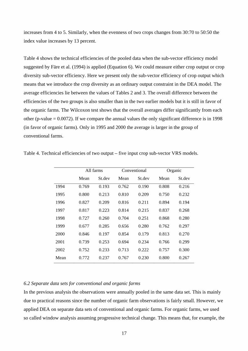
Table 4 shows the technical efficiencies of the pooled data when the sub-vector efficiency model

suggested by Färe et al. (1994) is applied (Equation 6). We could measure either crop output or crop

diversity sub-vector efficiency. Here we present only the sub-vector efficiency of crop output which

means that we introduce the crop diversity as an ordinary output constraint in the DEA model. The

average efficiencies lie between the values of Tables 2 and 3. The overall difference between the

efficiencies of the two groups is also smaller than in the two earlier models but it is still in favor of

the organic farms. The Wilcoxon test shows that the overall averages differ significantly from each

other (p-value = 0.0072). If we compare the annual values the only significant difference is in 1998

(in favor of organic farms). Only in 1995 and 2000 the average is larger in the group of

conventional farms.

Table 4. Technical efficiencies of two output – five input crop sub-vector VRS models.

All farms Conventional Organic

Mean St.dev Mean St.dev Mean St.dev

1994 0.769 0.193 0.762 0.190 0.808 0.216

1995 0.800 0.213 0.810 0.209 0.750 0.232

1996 0.827 0.209 0.816 0.211 0.894 0.194

1997 0.817 0.223 0.814 0.215 0.837 0.268

1998 0.727 0.260 0.704 0.251 0.868 0.280

1999 0.677 0.285 0.656 0.280 0.762 0.297

2000 0.846 0.197 0.854 0.179 0.813 0.270

2001 0.739 0.253 0.694 0.234 0.766 0.299

2002 0.752 0.233 0.713 0.222 0.757 0.300

Mean 0.772 0.237 0.767 0.230 0.800 0.267

6.2 Separate data sets for conventional and organic farms

In the previous analysis the observations were annually pooled in the same data set. This is mainly

due to practical reasons since the number of organic farm observations is fairly small. However, we

applied DEA on separate data sets of conventional and organic farms. For organic farms, we used

so called window analysis assuming progressive technical change. This means that, for example, the

17

efficiency scores for 1997 are calculated using the observations from 1994 to 1997 as the reference

set but the mean is calculated on the basis technical efficiencies of the farms observed in 199711.

Using several years’ observations as the reference set of organic farms increases the dimensions in

the DEA almost to the same level as in the annual analysis of conventional farms (without a

window).

The results for separate data sets for conventional and organic farms (window analysis for organic)

are presented in Tables 5 and 6. The means of these two groups are very close to each other but the

pattern of changes varies; in the group of conventional farms the average technical efficiencies are

at their lowest level in 1998 and 1999, and at their highest in 2000. In the group of organic farms,

efficiency decreases constantly since 1999. It seems that the variation in these two technologies is

somewhat different but this may be explained by the different ways of constructing the reference

sets.

Table 5. Technical efficiencies for conventional farms (annual reference sets).

1O5I 2O5I 2O5Isub

Mean St. dev Mean St. dev Mean St. dev

1997 0.771 0.177 0.911 0.095 0.832 0.177

1998 0.671 0.203 0.834 0.132 0.717 0.215

1999 0.663 0.241 0.872 0.129 0.735 0.246

2000 0.835 0.154 0.903 0.113 0.867 0.150

2001 0.728 0.189 0.878 0.115 0.789 0.190

2002 0.723 0.196 0.897 0.099 0.793 0.183

Mean 0.734 0.883 0.791

1O5I – one output, five input Farrell type model; 2O5I – two output, five input Farrell

type model; 2O5ICsub - two output, five input crop sub-vector efficiency model.

Table 6. Technical efficiencies for organic farms (reference sets of four year windows).

1O5I 2O5I 2O5Isub

Mean St. dev Mean St. dev Mean St. dev

1997 0.787 0.209 0.905 0.115 0.804 0.209

1998 0.749 0.282 0.933 0.086 0.812 0.269

1999 0.756 0.236 0.950 0.061 0.818 0.211

11 When we apply a four year window and assume technical progress we cannot calculate mean efficiencies in 1994- 1996.

18

2000 0.710 0.236 0.898 0.114 0.805 0.222

2001 0.734 0.240 0.882 0.133 0.780 0.230

2002 0.719 0.253 0.886 0.123 0.746 0.258

Mean 0.740 0.906 0.791

1O5I – one output, five input Farrell type model; 2O5I – two output, five input Farrell

type model; 2O5ICsub - two output, five input crop sub-vector efficiency model.

We should notice that the number of observations on which the annual average technical

efficiencies of organic farms are calculated, is only 14-2012. However, the results suggest that the

average efficiencies in the two technologies do not differ considerably when the reference group

applies the same technology, i.e., organic reference technology for organic farms and conventional

for conventional farms. The result is independent of the model the analysis is based upon. This

partially contradicts the result obtained when all farms were assumed to face the same technology,

i.e. the frontier of pooled reference set as presented in Tables 3 and 4, indicating the importance of

technology assumptions

7. Summary and Conclusions

We have estimated technical efficiencies for conventional and organic farms using data

envelopment analysis. When only traditional crop output is taken into account, conventional farms

prove to be technically more efficient than organic farms. A similar result has been obtained in

several studies (e.g., Oude Lansink et al., 2002) suggesting that conventional farms are more

productive than organic ones. Traditional technical efficiency analysis only accounts for market

inputs and outputs although the grounds for promotion of organic farming actually builds on the

demand of the society for non-market, environmental attributes.

The inclusion of crop diversity as another desirable output in the analysis leads to a relative increase

in technical efficiency of organic farms compared to conventional ones. Presuming the society to

prefer more diversity to less, for given crop output, conventional farms are no longer more efficient

than organic farms from the social point of view.

12 The number of annual observation in the last year of the window.

19

The Shannon crop diversity index used in comparison of conventional and organic practices in this

study has been an attempt to introduce another desirable output into the production process and

extend the analysis of different production technologies to a more comprehensive level. Further

research is needed in specifying possible inputs and outputs which should be taken into account in

the efficiency comparisons. In our analysis, we concentrated on the annual diversity variation at the

farm level. Regarding the evaluation of landscape values, the scale of analysis should, however,

exceed the borders of farm units. Therefore, the aggregation over farms and time become important

issues for policy assessments.

Even though our approach is only a first step towards analyzing simultaneously economic and

environmental impacts of alternative farming technologies, the overall message of our analysis is

clear. Normally, there is a trade-off between several outputs. Multiple outputs, including

environmental impacts, should be accounted for as the efficiency ranking of alternative

technologies is dependent on what is actually considered as outputs.

20

References

Armsworth, P.R., Kendall, B.E. & Davis, F.W. 2004. An introduction to biodiversity concepts

for environmental economists. Resource and Energy Economics 26: 115-136.

Baumgärtner, 2005. ‘Measuring the diversity of what? And for what purpose? A conceptual comparison of ecological and economic biodiversity indices’, Working Paper, University of Heidelberg. Biodiversity. 2005. Stanford Encyclopedia of Philosophy.

http://plato.stanford.edu/entries/biodiversity/, referred 8.12.2005)

Callicott, J.B., Crowder, L.B. & Mumford, M.R. 1999. Current normative concepts in

conservation. Conservation Biology 13: 22-35.

Chambers, R.G., Chung, Y. & Färe, R. 1998. Profit, directional distance function, and Nerlovian

efficiency. Journal of Optimization Theory and Applications 98(2): 351 - 364.

Charnes, A., Cooper, W.W. & Rhodes, E. 1978. Measuring the inefficiency of decision making

units. European Journal of Operational Research 2: 429 – 444.

Charnes, A., Clark, T., Cooper, W.W. & Golany, B. 1985. A developmental study of data

envelopment analysis in measuring efficiency of maintenance units in U.S. Air Forces. Annals of

Operational Research 2: 95-112.

Coelli, T., Rao, D.S.P. & Battese, G.E. 1998. An introduction to efficiency and productivity

analysis. Kluwer Academic Publishers.

Debreu, G. 1951. The coefficient of resource utilization. Econometrica 19(3): 273 – 292.

Di Falco, S. & Perrings, C. 2005. Crop biodiversity, risk management and the implications of

agricultural assistance. Ecological Economics 55: 459-466.

Dobbs, T.L. & Pretty, J.N. 2004. Agri-environmental stewardship schemes and

‘multifunctionality’. Review of Agricultural Economics 26(2): 220-237.

Farrell, M.J. 1957. The measurement of productive efficiency. Journal of the Royal Statistical

Society. Series A, 120: 253 – 281.

Färe, R., Grosskopf, S. & Lovell, C.A.K. 1994. Production frontiers. Cambridge.

Herzog, F., Steiner, B., Bailey, D., Baundry, J., Billeter, R., Bukácek, R., De Blust, G., De

Cock, R., Dirksen, J., Dormann, C.F., De Filippi, R., Frossard, E., Liira, J., Schmidt, T.,

Stöckli, C., Thenail, C., van Wingerden, W. & Bugter, R. 2006. Assessing the intensity of

temperate European agriculture at the landscape scale. European Journal of Agronomy 24: 165-181.

21

Hietala-Koivu, R., Lankoski, J. & Tarmi, S. 2004. Loss of biodiversity and its social cost in an

agricultural landscape. Agriculture, Ecosystem and Environment 103: 75-83.

Hole, D.G., Perkins, A.J., Wilson, J.D., Alexander, I.H., Grice, P.V. & Evans A.D. 2005. Does

organic farming benefit biodiversity? Biological Conservation 122: 113-130.

Karlen, D.L., Varvel, G.E., Bullock, D.G. & Cruse, R.M. 1994. Crop rotations for the 21st

century. Advanced Agronomy 53: 1-44.

Keylock, C.J. 2005. Simpson diversity and the Shannon-Wiener index as special cases of a

generalized entropy. Oikos 109(1): 203-207.

Koopmans, T.C. 1951. An analysis of production as an efficient combination of activities. In T.C.

Koopmans (ed.) Activity analysis of production and allocation. Cowles Commission for Research

in Economics. Monograph 13. New York. John Wiley and sons, Inc.

Latacz-Lohman, U. 2004. Dealing with limited information in designing and evaluating agri-

environmental policy. Paper presented in 90th EAAE seminar on 28.-29.10.2004, Rennes, France.

17 p.

McGarical, K. & Marks, B.J. 1995. FRAGSTATS: Spatial pattern analysis program for

quantifying landscape structure. USDA Forest Services. PNW-GTR-351. Portland, OR, USA.

Miettinen, A., Lehtonen, H. & Hietala-Koivu, R. 2004. On diversity effects of alternative

agricultural policy reforms in Finland: An agricultural sector modelling approach. Agricultural and

Food Science 13: 229-246.

Organic Farming in the EU: Facts and Figures, 2004.

(http://europa.eu.int/comm/agriculture/qual/organic/facts_en.pdf, referred 23.7.2004)

Oude Lansink, A., Pietola, K. & Bäckman, S. 2002. Efficiency and productivity of conventional

and organic farms in Finland 1994-1997. European Review of Agricultural Economics 29(1): 51-

65..

Pacini, C., Wossink, A., Giesen, G., Vazzana, C. & Huirne, R. 2003. Evaluation of sustainability

of organic, integrated and conventional farming systems: A farm and field-scale analysis.

Agriculture, Ecosystems and Environment 95: 273-288.

Ricci Maccarini, E. & Zanoli, A. 2004. Technical efficiency and economic performances of

organic and conventional livestock farms in Italy. Paper presented in 91st EAAE seminar on 24.-

25.9.2004, Crete, Greece. 28 p.

Riedell, W.E., Schumacher, T.E., Clay, S.A., Ellsbury, M.M., Pravecek,M. & Evenson, P.D.

1998. Corn and soil fertility responses to crop rotation with low, medium, or high inputs. Crop

Science 38: 427-433.

22

Shannon, C.E. 1948. A mathematical theory of communication. Bell System Technical Journal

27:379-423, 623-656.

Sipiläinen, T. 2003. Suurten maito- ja viljatilojen suorituskyky. Helsingin yliopisto. Taloustieteen

laitos. Julkaisuja 38.(In Finnish, English summary)

Sipiläinen, T., Oude Lansink, A. & Pietola, K. 2005. Learning in organic farming – An

application on Finnish dairy farms. Paper presented at the XIth Congress of EAAE, Copenhagen,

Denmark, August 24-27, 2005.

Stoltze, M., Piorr, A. Häring, A. & Dabbert, S. 2000. Environmtental impacts of organic farming

in Europe. Organic farming in Europe: Economics and Policy 6: 1-127.

Struik, P.C. & Bonciarelli, F. 1997. Resource use of cropping system level. European Journal of

Agronomy 7: 133-143.

Watson, C.A., Atkinson, D., Gosling, P. Jackson, L.R. & Rayns, F.W. 2002. Managing soil

fertility in organic farming systems. Soil Use Management 18: 239-247.

van Wenum, J.H., Wossink, G.A.A. & Renkema, J.A. 2004. Location specific modeling for

optimizing wildlife management on crop farms. Ecological Economist 48: 395-407.

Wossink, G.A.A. & van Wenum, J.H. 2003. Biodiversity conservation by farmers: analysis of

actual and contingent valuation. European Review of Agricultural Economics 30(4): 461-485.

Shephard, R.W. 1953. Cost and production functions. Princeton: Princeton University Press.

Shephard, R.W. 1970. Theory of cost and production functions. Princeton: Princeton University

Press.

23