effects of thermal conduction in microchannel gas...

Paper No. to be defined

1

Effects of Thermal Conduction

in Microchannel Gas Coolers for Carbon Dioxide

Pietro Asinaria, Luca Cecchinato

b, Ezio Fornasieri

*b

aDipartimento di Energetica, Politecnico di Torino, Corso Duca degli Abruzzi 24, I-10129 Torino, Italy

bDipartimento di Fisica Tecnica, Università degli Studi di Padova, via Venezia 1, I-35131 Padova, Italy

* Corresponding Author. Tel.: +39 049 827 6878; fax: +39 049 827 6896; e-mail: [email protected] - Member of

IIR Commission B2

Abstract

A numerical code was developed for an accurate fully three-dimensional simulation of

crossflow compact heat exchangers with finned, internally microchannelled flat tubes, which are

often used as gas coolers in transcritical refrigerating machines CO2 operated. The equations

describing the system were discretised by means of a finite-volume and finite-element hybrid

technique for strictly adhering to the real heat transfer process regarding the finned surfaces. The

numerical code uses recent correlations by different authors for predicting the heat transfer

coefficients both refrigerant side and air side. The results of simulations are verified against

experimental data reported in the open literature.

The aim of this work is to investigate the effects of thermal conduction inside metal on the

overall performance of the considered gas coolers; high-resolution meshes for the discretisation of

separating wall and fins makes it possible to avoid much of the approximations typical of the

traditional approaches. In particular the efficiency of finned surfaces, the real distribution of thermal

fluxes between the two fin roots and the effects of thermal conduction along the walls of

microchannel flat tubes are extensively discussed.

The numerical simulations confirm that the traditional approach for describing fins, which

assumes them as adiabatic at the middle section in order to decouple the equations accounting for

the effect of different temperatures at the fin roots, can be considered acceptable in a wide range of

applications. In a similar way, the conduction on fins along the direction of the air velocity and the

longitudinal conduction on tubes produce a negligible effect on the performance of the considered

class of heat exchangers.

Keywords: Refrigerant; Carbon Dioxide; Transcritical cycle; Gas Cooling; Design; Heat Exchangers; Modeling.

mailto:[email protected]


2

1. Introduction

Finned heat exchangers made of flat extruded aluminium tubes with internal microchannels are

a topical subject, both from the technological and the scientific point of view. With respect to the

traditional finned coil heat exchangers, they appear to have a better energy efficiency, in terms of

larger heat transfer capability being the same the mechanical power spent for circulation of the

working fluids. This is true both for the inside and outside sides of the heat exhanger.

Furthermore, microchannel tubes, because of their high mechanical resistance to the internal

pressure, are a suitable solution for gas cooling in CO2 transcritical cycles. The optimisation of this

type of heat exchanger is therefore one of the main research goal for the development of

refrigerating systems operated by this natural fluid.

The CO2 transcritical cycle differs much from a traditional vapour compression cycle: a

fundamental difference is that the upper pressure is not any longer related to heat transfer condtions

of a condenser, but is a parameter subjected to optimisation since its value, as well as the gas

temperature at the throttling valve inlet, has a great impact on the thermodinamic efficiency of the

cycle. High thermal efficiency of gas cooler is an essential condition to obtain high COP values,

since a low value of the CO2 temperature at its outlet increases the cooling capacity, so allowing a

reduction of the upper pressure and thus of the mechanical compression power. In fact, the optimal

upper pressure value can be regarded, at a rough estimate, as inversely proportional to the gas

cooler thermal efficiency.

The gas cooler analysis, aimed at optimising its design, faces the problem related to the wide

variations of the thermodinamical and thermophysical properties near the critical point: using a

high-resolution mesh is the mandatory solution.

The aim of this work is to analyse the possible drawbacks of the common assumptions used to

simplify the solution of the equations related to conduction inside metal. To this end, a code was

developed, which takes into account the real distribution of heat flux due to transverse and

longitudinal conduction along both tubes and fins. In the following sections, the physical model and

the implemented discretisation will be illustrated and some results of a simulation will be discussed.

2. The numerical code

Since crossflow compact heat exchangers with microchannelled flat tubes provide high thermal

efficiency, they are widely utilised as gas coolers in transcritical refrigeration machines with CO2 as

the operating fluid [1]. These components conceptually belong to the general class of crossflow heat

exchangers and they look as the one shown in Fig. 1(a).

For convenience, the calculation domain is subdivided into a wall domain w , which identifies

all metal parts, and a fluid domain f , which identifies all volumes containing fluids. The fluid

domain is constituted by many fluid paths, each one characterised by a proper dimensionless

coordinate 1/0 iii lXx . The physical model, defined over the whole computation domain, is

expressed by the following equations.

fP ix

iiiiiwiiiii dyAyTyThxhG0

)()()0()( (1)

i

i

ii

i

i

i

iiid

xlf

Gxpp

2)()0(

2

(2)

wP 0)( ww Tk (3)


3

The overall thermal balance for the heat exchanger can be expressed as:

0)1()0()0()1()(

hc

N

ij

jjj

N

ii

iiiww PPhhGhhGdVTkh

w

c

(4)

For solving the system of equations (1), (2), (3) and (4), a proper set of boundary conditions is

needed. Usually for equations (1) and (2), Dirichlet-type conditions at the fluid inlet for enthalpy

)0(ih and pressure )0(ip are imposed. On the other hand for equation (3), a Neumann-type

condition is imposed on the portion of the wall surface A which is in contact with the external

environment. Since the heat exchangers are usually well insulated, a zero value is set for this heat

flux ( 0/ nTw for AP w ). The phenomenological coefficients which characterise heat

transfer ( i ) and pressure drops ( if and i ) are evaluated according to common correlations

reported in the open literature (see Tab. 1).

The described physical model is characterised by strong coupling among equations, mainly due

to equation (3), which depends on the temperature profile inside the metallic walls. According to

the purpose of this work, the effects of thermal conduction is investigated without any simplifying

hypothesis regarding the coupling of equations. Recently, a general numerical approach for heat

exchangers, dubbed Semi-Explicit Method for Wall Temperature Linked Equations SEWTLE, has

been proposed [7]. This method decouples the calculation of the wall temperature field from that of

fluid temperature and computes the final solution by means of an iterative procedure which is

brought to convergence by verifying the enthalpy balance between hot-side and cold-side. In

particular, a guess profile for temperature inside metallic wall is assumed as the starting point; on

this basis, the convective thermal fluxes is calculated by means of equations (1) and (2). Then a new

distribution of wall temperature, which will be closer to final solution, is determined by equation

(3). This iterative procedure continues until the condition (4) is satisfied within the desired

tolerance.

In order to create a numerical code for simulating the physical model, a discretisation technique

must be considered. According to the Finite Volume Method (FVM) [8], the flat tubes are

discretised into elementary control volumes, characterized by centroids located at intersections

between the fins and the separating walls that identify microchannels, as shown in Fig. 1(b). The

same techniques is applied to the fluid domain: numerical convenience suggests to introduce a

transversal dislocation between fluid and tube centroids [9], as shown in Fig. 1(c). The application

of the FVM to fins discretisation would increase beyond reasonableness the number of nodal values

in order to obtain a sound accuracy: for this reason the Finite Element Method (FEM) was

employed. Unfortunately, the technique of classical surrounded elements does not ensure the

thermal continuity needed by the SEWTLE approach. Then an intrinsically conservative element

was introduced for the FEM definition of fins, as shown in Fig. 2(a), which is compatible with the

SEWTLE technique [9], since the shape function (5) coincides with the exact solution of the

equations of the convective heat transfer in fins, under some simplifying hypotheses [10].

)exp()exp()exp()exp(),( 4321 zCzCyCyCzy (5)

where )( skwi is the inverse of a characteristic length and

iiiw TzyTzy ),(),( represents the effective temperature difference. The couple of

temperature at fin roots and the conductive heat fluxes at remaining borders constitute a proper set

of boundary conditions to calculate the constants iC . In particular this set makes the element

intrinsically conservative and produces an accurate description of temperature profile, as shown in

Fig. 2(b).


4

The described discretisation scheme is an hybrid one, which adopts both FVM and FEM to

avoid simplifying hypotheses, providing therefore high accuracy, without demanding too much

calculation resources.

3. Comparison with experimental data

In order to verify the reliability of the numerical code, a comparison between simulation results

and experimental data was carried out. The experimental data were found in [11] and cover a wide

range of operating conditions of the gas-cooler for automotive applications depicted in Fig. 3. The

simulation speed and the results accuracy depend on the number of nodes of the grid in the section

of microchannelled tube; the best definition is the one that considers the number of virtual

microchannels equal to the real case, but a smaller number can be chosen for simplifying the

calculation.

In Fig. 4, the calculated values of the total heat transfer rate are reported against the

experimental values; the simulation slightly overestimate the real thermal performance, but the

accuracy is high, since most of the errors are smaller than 3%, being the maximum error around 6%.

Even if from these results the simulation model appears reliable and accurate, it is worth noting that

this high accuracy could be related to the high thermal efficiency of the gas cooler, that makes the

thermal power not very sensitive to the heat transfer characteristics. Furthermore, the total heat flow

exchanged is strongly dependent on the correlations chosen to evaluate the heat transfer

coefficients. On the other hand, applying the direct numerical analysis of convective heat transfer

has been considered impractical, because it would have required a tremendous increase in the mesh

size.

It is interesting to investigate the effect of the mesh resolution on the final results, since in

transcritical CO2 cycles the modelling of the cooling process at high pressure raises some problems

related to transformation close to the critical point, where very large variations of the

thermodynamical and thermophysical properties occur.

To this end, a dimensionless parameter, 2211 crincrin hhppD , was proposed by

the authors to quantify the proximity of the operating conditions to the critical point.

Although the error distribution is quite scattered, as shown in Fig. 4(b), the trend curve with

reasonable accuracy can be described by eq. (6) which clearly demonstrates that errors increase

when the system is operating near the critical point:

)/exp( 00 DDEE (6)

To analyse the sensitivity of the simulation errors to the mesh resolution, the calculation for

Test n° 9 [11], which is a critical case for the operating conditions, was repeated, increasing the

number of nodes from the most simplified case. Increasing the number of nodes brings about a

better accuracy in representing the thermal fields in the system and from a physical point of view is

equivalent to increase the number of virtual microchannels inside the flat tube. When the number of

virtual microchannels is equal to the real number of microchannels in the gas cooler, the maximum

possible accuracy is reached. The results of this comparison are shown in Tab. 2; increasing the

number of virtual channels from 1 to 3 greatly improves the accuracy in evaluating heat flow, but a

further increase in the mesh resolution does not produce a significant benefit. In the same Tab. 2 the

total heat flow was subdivided into three contributions, referring to the three sections of the heat

exchanger, corresponding to the three gas passages; the deviations of the calculated values for

different numbers of virtual channels with respect to the most simplified case (one virtual channel)

can give an account of the effect of the mesh size on the heat transfer prediction for heat exchanger

of different effectiveness, or subjected to different heat flow: as expected, when comparing the


5

deviations for Section I and for the whole heat exchanger, high heat flux calls for high resolution,

because the consequent high temperature gradients require more detail in describing the process.

As far as the pressure drop of the refrigerant is concerned, in [12] it is asserted that the most of

the traditional correlations underestimate the experimental data: this has been confirmed by the

results of the simulations, which show an average mean error of –70% in predicting pressure drop.

To investigate the effect of this variable on heat flow, simulations have been carried out having

increased, according to different multiplying factors, the values of pressure drop calculated from the

correlations reported in Tab. 1. The results in Tab. 3 point out small improvement in the prediction

of heat flow and highlight small sensitivity of the heat transfer performance to pressure drops.

4. The thermal conduction in fins

The numerical code described in the previous sections can investigate some phenomena usually

neglected in evaluating the fins efficiency. In modelling compact heat exchangers as the one shown

in Fig. 1, an usual approximation is employed, consisting in the half-fin-length idealisation.

According to this idealisation, the section of the fin at the middle distance from the tubes is assumed

as adiabatic; this is strictly true only when the fin bases are both at the same temperature. In a real

case, these temperatures in general are different and, as a consequence, the adiabatic line is shifted

from the middle position and unequal lengths of fin transport heat to the tubes at its roots. In

extreme cases, the adiabatic line is not present on the fin and the two tubes are subjected to opposite

heat flows (entering one tube and exiting from the other).

The transverse heat flows for unit length Aq and Bq at fin roots A and B can respectively be

expressed by the following correlations [13]:

BAwABAwA kz

syqzk

z

syq

)sinh(

2)()cosh(

)sinh(

2)(

0

*

0

0

(7)

BAwBABwB kz

syqzk

z

syq

)sinh(

2)()cosh(

)sinh(

2)(

0

*

0

0

(8)

where 0z is the fin height, *

Aq and *

Bq the heat flows per unit length predicted by the half-fin-

length idealisation. To discuss the adequacy of this idealisation, a splitting factor is introduced:

00

00

)()()(

y

BA

y

A dyyqyqdyyqr (9)

where the heat flows due to thermal conduction is considered positive if entering the fin. The

half-fin-length idealisation is exactly complying with reality when the temperature differences at

both ends are equal BA ; in this case the splitting factor is 2/1r . For most of the typical

operating conditions of multi-stream plate fin heat exchangers, this condition is very close to be

fulfilled and half-fin-length approximation produces acceptable errors. When A greatly differs from

B, the splitting factor are far from 1/2 and therefore in these cases the half-fin-length idealisation is

not any longer acceptable.

Another approximation widely employed in modelling heat transfer with extended surfaces

suggests to neglect the thermal conduction directed along the direction of air flow. For louvered

fins, the longitudinal conduction can be taken into account through a suitable value of an equivalent

directional thermal conductivity.


6

To show the potential of the present numerical code and to verifying the accuracy of the

simplifying hypotheses of common use, a simulation was performed for the compact heat exchanger

shown in Fig. 3. In particular Test n° 32 [11] is considered: the mass flow rate of carbon dioxide is

26 sg / , the inlet pressure is 76 bar and the inlet temperature is 78.2 C , while for air the mass

flow rate is 454 sg / and the inlet temperature is 26.8 C .

In Fig. 5 the contour lines of the splitting factor are reported for the face area of the heat

exchanger; this variable is not defined in all point of the face area, but only for fins and

consequently the curves are built by linking points located on the fins; moreover, in the definition of

splitting factor (9), subscript A refers to the upper fin root, so that 2/1r means that the upper

thermal flux is greater than lower one.

Only few fins are characterized by splitting factors far from ideal value 2/1r ; they are

located between flat tubes which are close to different refrigerant passages, where the temperature

difference between the refrigerant flowing inside adjacent tubes is large. In this situation the half-

fin-length idealisation introduces a significant error in estimating the distribution of thermal fluxes

and the related temperature field inside the metal. However since BABA qqqq ** , as follows

from equations (8) and (9), it can be concluded that the half-fin-length idealisation correctly

predicts the total heat transfer from/to a fin, but it is wrong in predicting the individual heat flows at

the roots. This involves a modest effect on the prediction of the total heat transfer rate, as results

from Tab. 4.

In Fig. 6 some relevant values of the thermal variables are shown for different section of a fin,

subdivided into vertical strips linking two adjacent tubes. The values inside the circles show the

convective heat flow exchanged with air on both fin sides. The values at the fin root show the heat

flow entering (negative value) or exiting (positive values) from the tubes; the values inside

parentheses refer to heat flow predicted by half-fin-length idealisation. The temperatures at the fin

roots are printed outside the fin contour. The longitudinal heat flow transferred by conduction is

indicated next the related arrows. For the considered fin, the splitting factor is equal to 47.2r ,

which is very close to maximum value in Fig. 5, and entails a reversed conductive flux (i.e. from the

fin to the tube) at the lower fin root. The sum of heat flow entering both the fin bases is equal to

440 mW, as predicted by half-fin-length idealisation, according to theory. The longitudinal

conductive heat flow in the direction of the air flow shows its maximum at the central portion of the

fin, while is very small at both fin ends; anyway the maximum value, which is equal to 12 mW , is

nearly negligible if compared with the transverse conductive heat flow.

5. The thermal conduction in microchannelled tubes

It is common practice to consider the wall temperature of the tubes uniform on any cross

section and to neglect the heat flowing longitudinally by conduction through the walls, even if

longitudinal temperature gradients exists. Instead, the present simulation code takes into account

these aspects of heat transfer and therefore can quantify the error associated to the mentioned

simplifying assumptions.

In the following Figg. 7 and 8 some of the numerical results obtained with the simulation code

are reported, referring to the operating conditions of Test n° 32 [11], already considered in Fig. 5.

A factor has been defined to take into account the non-uniformity of the temperature field in

the cross section of microchannel tubes:

N N N N

i i i i i ii i i i

A T A T A A

2

1 1 1 1

(10)


7

The contour lines of factor for the cross sections of microchannel tubes are plotted in Fig. 7.

Notwithstanding the factor is a variable defined only for the tube section, for the sake of

readability, the curves are built by linking all points with equal values (the same for the following

Fig. 8).

According to heat flux resulting from simulation, compared with the one of an ideal case with

isothermal cross section, it follows that the common assumptions can be considered fully

acceptable. This holds also for most critical sections located at the inlet of refrigerant where there is

the maximum temperature differences between the fluids and consequently the maximum heat flux.

In Fig. 8 the contours lines of the longitudinal heat flow by conduction along the tube walls (in

the direction of the refrigerant flow) are plotted. The numerical results of Fig. 8 show that the

longitudinal heat flow can be neglected in evaluating the heat transfer process in such a kind of heat

exchanger, also for the tubes subject to the maximum temperature gradients. In fact, the order of

magnitude of the overall heat flow for a single tube is about one hundred Watt.

6. Final remarks

At last, a sensitivity analysis has been carried out about the influence of the heat transfer

coefficients and the thermal conductivity of the metal for both fins and tubes on the heat transfer

capability of the heat exchanger; to this purpose simulations were performed, increasing these

parameters by 20%, one at a time. The results of simulations reported in Tab. 5 show that the

increase in the air side heat transfer coefficient has comparatively the largest effect because it acts

on the side where the largest thermal resistance exists, but this effect is nevertheless rather small,

because of the high thermal efficiency of the heat exchanger.

To complete the analysis of the effect of the thermal conduction inside the metal, with

reference to the simplifications assumed in the traditional numerical codes, other simulations have

been performed, setting to zero, one at a time, the thermal conductivity along different axes,

excepting the one orthogonal to the fin bases. From the results, shown in Tab. 6, it can be inferred

that the longitudinal conduction, both in fins and tubes, and the transverse conduction in tubes are

not significant for thermal process; thence it results that the traditional calculation procedures, even

if they do not take into account these effects, nevertheless do not suffer any significant loss of

accuracy in relation to these simplifications.

Conclusions

A numerical simulation model for compact heat exchangers which takes into account the effect

of thermal conduction along the fins and the walls of tubes was developed to analyse the effect of

the simplifying assumption used in the classical approach.

The conclusions drawn from the analyses are:

a) The models using the half-fin length idealisation, although do not accurately represent

the real distribution of heat flow between the fin roots, when the temperatures at the fin

bases are different, nevertheless give a reasonably accurate prediction of the total heat

flow exchanged.

b) The longitudinal conduction in fins, the transverse and the longitudinal conduction in

tubes give negligible effects on the total heat flow and on the temperature field.

The innovative numerical code here presented certainly offers improved accuracy, with respect

to the simplified simulation models, in predicting the thermal variables and the total heat flow:

although in most cases the accuracy of the simplified models can be regarded as acceptable, when


8

thermal conduction assumes a key role in determining the heat flow (low metal thermal

conductivity, low wall thickness, high convective heat transfer coefficients) there is a need for a

more sophisticated modelisation, as the one described in the present paper.

Nomenclature

A area [m

2] s fin thickness [m]

d hydraulic diameter [m] V volume [m3]

f friction factor for distributed pressure drop [-] T temperature [K]

G mass flow rate [kg/s] convective heat transfer coefficient [W/(m

2K)]

h specific enthalpy [J/kg] friction factor for concentrated pressure drop

[-]

k thermal conductivity [W/(mK)] density [kg/m3]

P heat flow [W] temperature field variance [K]

p pressure [Pa] The inverse of a characteristic length [1/m]

q Heat flow for unit length [W/m] Effective temperature difference [K]

r splitting factor [-]

Subscripts:

w wall

f fin

i, in inlet

cr critical


9

References

[1] McEnaney R. P., Park Y. C., Yin J. M., ,Hrnjak P. S.: Performance of the prototype of

transcritical R-744 mobile A/C system, SAE International Congress and Exposition, Paper

1999-01-0872, 1999.

[2] Chang Y., J. Wang C. C.: A generalized heat transfer correlation for louver fin geometry,

International Journal of Heat and Mass Transfer, vol. 40, n 3, pp. 533-544, 1997.

[3] Chang Y., J. Wang C. C.: Air side performance of brazed aluminium heat exchangers, Journal

of Enhanced Heat Transfer, vol. 3, n 1, pp. 15-28, 1996.

[4] Idelchik E., Handbook of Hydraulic Resistance, 3rd Edition, CRC Press, 1994.

[5] Gnielinski V.: New equations for heat and mass transfer in turbulent pipe and channel flow,

International Chemical Engineering, vol. 16, pp. 359-368, 1976.

[6] Churchill S. W.: Friction-factor equation spans all fluid flow regimes, Chemical Engineering,

vol. 7, pp. 91-92, 1977.

[7] Corberan J. M., De Cordoba P. F., Gonzalvez J., Alias F.: Semiexplicit Method for Wall

Temperature Linked Equations (SEWTLE): a General Finite-Volume Technique for the

Calculation of complex Heat Exchangers, Numerical Heat Transfer: Part B, vol. 40, pp. 37-

59, 2001.

[8] Patankar S. V.: Numerical Heat Transfer and Fluid Flow, Hemisphere, New York, 1980.

[9] Asinari P., Finite-Volume and Finite-Element Hybrid Technique for the Calculation of

Complex Heat Exchangers by Semi-Explicit Method for Wall Temperature Linked Equations

(SEWTLE), to be published on Numerical Heat Transfer: Part B, 2003.

[10] Kern D. Q., Kraus A. D.: Extended Surface Heat Transfer, McGraw-Hill, New York, 1994.

[11] Yin J. M., Bullard C. W., Hrnjak P. S.: R-744 gas cooler model development and validation,

International Journal of Refrigeration, vol. 24, pp. 692-701, 2001.

[12] Rieberer R.: CO2 properties, IIR Workshop on CO2 Technology in Refrigeration, Heat Pump

and Air Conditioning Systems, Mainz, Germany, 1999.

[13] Prasad B. S. V.: Fin Efficiency and Mechanisms of Heat Exchange Through Fins in Multi-

Streams Plate-Fin Heat Exchangers: Formulation, International Journal of Heat and Mass

Transfer, vol. 39, n 2, pp. 419-428, 1996.


10

Figure Captions

Figure 1. (a) Generic element of compact crossflow heat exchanger. (b) Plan view of control

volume centroids. (c) Isometric view of control volume centroids.

Figure 2. (a) Intrinsically conservative element for fin discretisation. (b) Three-dimensional plot of

fin temperature field by intrinsically conservative elements.

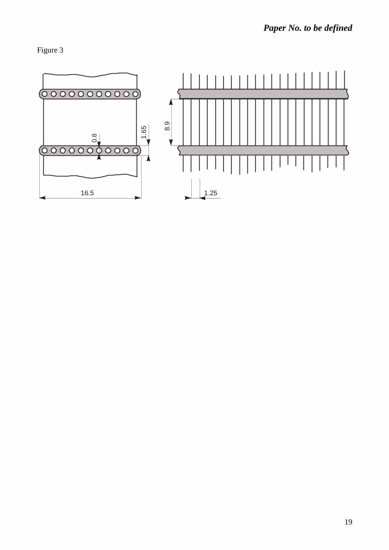
Figure 3. Basic geometry of the considered heat exchanger. The frontal area is equal to 545 x 350

)(h mm . The number of flat tubes is equal to 34 and they are subdivided into 3 passages [11].

Figure 4. Comparison between total heat flow calculated by numerical code and experimental data

[11]. (a) Simulations performed with detailed meshes: Test n° 9, n° 32 and n° 37. (b) Correlation

between error and factor E accounting for operation near the critical point.

Figure 5. Contour lines of the splitting factor for conductive heat flow at fin roots (air side frontal

view, XZ plane in Fig. 1).

Figure 6. Thermal variables in a fin ( 47.2r ) located between the first and the second passage.

Black arrows refer to conductive heat flows (transverse and longitudinal). Values inside circles refer

to convective thermal fluxes. Values inside parentheses refer to half-fin-length idealisation.

Figure 7. Contour lines of parameter (temperature variance in the cross sections of flat tubes)

(air side frontal view, XZ plane in Fig. 1).

Figure 8. Contours lines of longitudinal conductive heat flow in flat tubes (air side frontal view,

XZ plane in Fig. 1).


11

List of Tables

Table 1

Phenomenological coefficients used in numerical code.

Heat Transfer Pressure Drop

Localized Distributed

[W/m2K] f [-] [-]

Air Chang e Wang, 1997 [2] Chang e Wang, 1996 [3] Idelchik, 1994 [4]

CO2 Gnielinski, 1976 [5] Churchill, 1977 [6] Idelchik, 1994 [4]


12

Table 2

Effects of mesh resolution on transferred thermal power.

TEST

[11]

Virtual

Micro

channels

Transferred Thermal Power

Measured (1) Code (2) I II III Error (2)/(1)

[W] [W] [W] [W] [W] [%]

Test n° 9 1 3643 4041 2418 1027 595 +10.9

Test n° 9 3 3643 3887 2354 976 557 +6.7

Test n° 9 5 3643 3872 2324 975 572 +6.3

Test n° 9 7 3643 3820 2250 975 595 +4.9

Test n° 9 9 3643 3836 2251 978 607 +5.3

Test n° 9 11 3643 3845 2251 987 607 +5.5


13

Table 3

Effects of pressure drops on transferred thermal power.

TEST

[11]

Pressure

Drops


Measured (1) Code (2) Error (2)/(1)

[W] [W] [%]

Test n° 9 p (Tab. 1) 3643 4041 +10.9

Test n° 9 p2 3643 4022 +10.4

Test n° 9 p3 3643 4002 +9.9

Test n° 9 p4 3643 3983 +9.3


14

Table 4

Effects of different assumptions in fin modelling on transferred thermal power.

TEST

[11]

Fin Modeling Transferred Thermal Power

Measured (1) Code (2) Error (2)/(1)

[W] [W] [%]

Test n° 27 Half-Fin-Length

Idealization

3285 3420 +4.1

Test n° 27 Improved

Temperature Field

3285 3385 +3.0


Idealization

3596 3918 +9.0


Temperature Field

3596 3879 +7.9


Idealization

3138 3353 +6.9


Temperature Field

3138 3327 +6.0


15

Table 5

Effects of heat transfer coefficients on transferred thermal power.

TEST

[11]

Heat Transfer

Coefficients


Measured (1) Code (2) Variation (2)/(1)

[W] [W] [%]

Test n° 11 Reference 4774 4845 +1.5

Test n° 11 e +20% - 4897 +2.6

Test n° 11 i +20% - 4848 +1.6

Test n° 11 +20% - 4843 +1.4


Test n° 32 e +20% - 4079 +13.4

Test n° 32 i +20% - 3895 +8.3

Test n° 32 +20% - 3882 +8.0


16

Table 6

Effects of conduction modelling on transferred thermal power.

TEST

[11]

Conduction

Modeling


Measured (1) Code (2) Variation (2)/(1)

[W] [W] [%]


Test n° 11 No Conduction

Longitudinal Fin

- 4844 +1.5


Longitudinal Tube

- 4845 +1.5


Transverse Tube

- 4843 +1.4



Longitudinal Fin

- 3879 +7.9


Longitudinal Tube

- 3882 +8.0


Transverse Tube

- 3878 +7.8


17

List of figures

Figure 1


18

Figure 2


19

Figure 3

1.25

0.8

16.5

1.6

5

8.9


20

Figure 4


21

Figure 5


22

Figure 6


23

Figure 7


24

Figure 8

effects of thermal conduction in microchannel gas...

Documents