effects of phase and amplitude errors on qam …

Clemson UniversityTigerPrints

All Theses Theses

8-2009

EFFECTS OF PHASE AND AMPLITUDEERRORS ON QAM SYSTEMS WITH ERROR-CONTROL CODING AND SOFT DECISIONDECODINGJason EllisClemson University, [email protected]

Follow this and additional works at: https://tigerprints.clemson.edu/all_theses

Part of the Electrical and Computer Engineering Commons

This Thesis is brought to you for free and open access by the Theses at TigerPrints. It has been accepted for inclusion in All Theses by an authorizedadministrator of TigerPrints. For more information, please contact [email protected].

Recommended CitationEllis, Jason, "EFFECTS OF PHASE AND AMPLITUDE ERRORS ON QAM SYSTEMS WITH ERROR-CONTROL CODINGAND SOFT DECISION DECODING" (2009). All Theses. 649.https://tigerprints.clemson.edu/all_theses/649

https://tigerprints.clemson.edu?utm_source=tigerprints.clemson.edu%2Fall_theses%2F649&utm_medium=PDF&utm_campaign=PDFCoverPages

https://tigerprints.clemson.edu/all_theses?utm_source=tigerprints.clemson.edu%2Fall_theses%2F649&utm_medium=PDF&utm_campaign=PDFCoverPages

https://tigerprints.clemson.edu/theses?utm_source=tigerprints.clemson.edu%2Fall_theses%2F649&utm_medium=PDF&utm_campaign=PDFCoverPages

https://tigerprints.clemson.edu/all_theses?utm_source=tigerprints.clemson.edu%2Fall_theses%2F649&utm_medium=PDF&utm_campaign=PDFCoverPages

http://network.bepress.com/hgg/discipline/266?utm_source=tigerprints.clemson.edu%2Fall_theses%2F649&utm_medium=PDF&utm_campaign=PDFCoverPages

https://tigerprints.clemson.edu/all_theses/649?utm_source=tigerprints.clemson.edu%2Fall_theses%2F649&utm_medium=PDF&utm_campaign=PDFCoverPages

mailto:[email protected]

EFFECTS OF PHASE AND AMPLITUDE ERRORS ONQAM SYSTEMS WITH ERROR-CONTROL CODING AND

SOFT-DECISION DECODING

A ThesisPresented to

the Graduate School ofClemson University

In Partial Fulfillmentof the Requirements for the Degree

Master of ScienceElectrical Engineering

byJason D. EllisAugust 2009

Accepted by:Dr. Michael Pursley, Committee Chair

Dr. Daniel NoneakerDr. Harlan Russell

ABSTRACT

Demodulation of M-ary quadrature amplitude modulation (M-QAM) requires the

receiver to estimate the phase and amplitude of the received signal. The demodulator

performance is sensitive to errors in these estimates, and the sensitivity increases as M

increases. We examine the effects of phase and amplitude errors on the performance

of QAM communication systems with error-control coding and soft-decision decoding.

A mathematical analysis of these effects is presented for two soft-decision decoding

metrics. Performance comparisons are given for 16-QAM and 64-QAM for two error-

control coding techniques and two soft-decision decoding metrics.

ACKNOWLEDGMENTS

I would like to thank my advisor, Dr. Michael B. Pursley, for all of his assistance

in the preparation of this thesis. I am very grateful for all of the guidance and support

that he has given me during my graduate education, and I look forward to continued

success working under his advisement. I would like to thank Dr. Daniel L. Noneaker

and Dr. Harlan B. Russell for their generous efforts in serving on my committee. I

am very grateful for the support that they have shown me and the roles that they

have played in my success here at Clemson.

I would also like to thank family and friends for their love, prayers, and support.

I am truly blessed to have such wonderful people in my life.

TABLE OF CONTENTS

Page

TITLE PAGE . . . . . . . . . . . . . . . . . . . . . . . . . . . . . . . . . i

ABSTRACT . . . . . . . . . . . . . . . . . . . . . . . . . . . . . . . . . . ii

ACKNOWLEDGMENTS . . . . . . . . . . . . . . . . . . . . . . . . . . . iii

LIST OF TABLES . . . . . . . . . . . . . . . . . . . . . . . . . . . . . . . vi

LIST OF FIGURES . . . . . . . . . . . . . . . . . . . . . . . . . . . . . . viii

CHAPTER

1. Introduction . . . . . . . . . . . . . . . . . . . . . . . . . . . . . 1

2. Phase and Amplitude Errors . . . . . . . . . . . . . . . . . . . . 3

2.1 Phase Error . . . . . . . . . . . . . . . . . . . . . . . . . . . 32.2 Amplitude Error . . . . . . . . . . . . . . . . . . . . . . . . 7

3. Log Likelihood Ratio Metric . . . . . . . . . . . . . . . . . . . . 10

3.1 Mathematical Analysis of a Phase Error . . . . . . . . . . . 113.2 Mathematical Analysis of an Amplitude Error . . . . . . . . 17

4. Distance Metric . . . . . . . . . . . . . . . . . . . . . . . . . . . 22

4.1 Mathematical Analysis of a Phase Error . . . . . . . . . . . 234.2 Mathematical Analysis of an Amplitude Error . . . . . . . . 27

5. Performance Analysis . . . . . . . . . . . . . . . . . . . . . . . . 30

5.1 Performance Results for a System with a Phase Error . . . 305.2 Performance Results for a System with an Ampli-

tude Error . . . . . . . . . . . . . . . . . . . . . . . . . . . 37

Table of Contents (Continued)

Page

6. Conclusion . . . . . . . . . . . . . . . . . . . . . . . . . . . . . . 44

v

LIST OF TABLES

Table Page

2.1 Required ENR for a symbol error probability of 10−5 in a16-QAM system. . . . . . . . . . . . . . . . . . . . . . . . . . . . . . 6

2.2 Required ENR for a symbol error probability of 10−5 in a16-QAM system. . . . . . . . . . . . . . . . . . . . . . . . . . . . . . 9

3.1 Slopes of LLR metrics for 16-QAM with zero phase error. . . . . . . 14

3.2 Average slope magnitudes of LLR metrics for 16-QAM withzero phase error. . . . . . . . . . . . . . . . . . . . . . . . . . . . . . 15

3.3 LLR slope magnitudes for an interior point in a 16-QAM sys-tem with zero phase error. . . . . . . . . . . . . . . . . . . . . . . . 16

3.4 Normalized LLR slope magnitudes for an interior point in a16-QAM system with zero phase error. . . . . . . . . . . . . . . . . . 16

3.5 Normalized LLR slope magnitudes for a corner point in a 16-QAM system with zero phase error. . . . . . . . . . . . . . . . . . . 17

3.6 Normalized LLR slope magnitudes for an other exterior pointin a 16-QAM system with zero phase error. . . . . . . . . . . . . . . 17

3.7 Slopes of LLR metrics with a gain factor of unity. . . . . . . . . . . 19

3.8 LLR slope magnitudes for an interior point in a 16-QAM sys-tem with a gain factor of unity. . . . . . . . . . . . . . . . . . . . . . 19

3.9 Normalized LLR slope magnitudes for an interior point in a16-QAM system with a gain factor of unity. . . . . . . . . . . . . . . 20

3.10 Normalized LLR slope magnitudes for a corner point in a 16-QAM system with a gain factor of unity. . . . . . . . . . . . . . . . 20

3.11 Normalized LLR slope magnitudes for an other exterior pointin a 16-QAM system with a gain factor of unity. . . . . . . . . . . . 21

4.1 Slopes of distance metrics with zero phase error. . . . . . . . . . . . 25

List of Tables (Continued)

Table Page

4.2 Distance metric slope magnitudes for an interior point in a16-QAM system with zero phase error. . . . . . . . . . . . . . . . . . 25

4.3 Distance metric slope magnitudes for a corner point in a 16-QAM system with zero phase error. . . . . . . . . . . . . . . . . . . 26

4.4 Distance metric slope magnitudes for an other exterior pointin a 16-QAM system with zero phase error. . . . . . . . . . . . . . . 26

4.5 Slopes of distance metrics with a gain factor of unity. . . . . . . . . 28

4.6 Distance metric slope magnitudes for an interior point in a16-QAM system with a gain factor of unity. . . . . . . . . . . . . . . 28

4.7 Distance metric slope magnitudes for a corner point in a 16-QAM system with a gain factor of unity. . . . . . . . . . . . . . . . 29

4.8 Distance metric slope magnitudes for an other exterior pointin a 16-QAM system with a gain factor of unity. . . . . . . . . . . . 29

vii

LIST OF FIGURES

Figure Page

2.1 Inphase-quadrature coherent correlation receiver used for QAMdemodulation. . . . . . . . . . . . . . . . . . . . . . . . . . . . . . . 4

2.2 16-QAM signal constellation and decision boundaries for asystem with no phase error and a constellation with a 5◦ phaseerror. . . . . . . . . . . . . . . . . . . . . . . . . . . . . . . . . . . . 4

2.3 16-QAM signal constellation and maximum likelihood deci-sion boundaries. . . . . . . . . . . . . . . . . . . . . . . . . . . . . . 8

2.4 Receiver’s estimate of a 16-QAM signal constellation and de-cision boundaries for a system with β = 1.1. . . . . . . . . . . . . . . 8

3.1 Possible received points near a QAM output signal. . . . . . . . . . 14

5.1 Required ENR to achieve a 10−2 packet error probability asa function of the phase error . . . . . . . . . . . . . . . . . . . . . . 31

5.2 Packet error probabilities for several values of the phase errorin a 16-QAM system with the convolutional code and thedistance metric. . . . . . . . . . . . . . . . . . . . . . . . . . . . . . 32

5.3 Packet error probabilities for several values of the phase errorin a 16-QAM system with the convolutional code and the LLRmetric. . . . . . . . . . . . . . . . . . . . . . . . . . . . . . . . . . . 32

5.4 Packet error probabilities for several values of the phase errorin a 16-QAM system with the turbo product code and thedistance metric. . . . . . . . . . . . . . . . . . . . . . . . . . . . . . 33

5.5 Packet error probabilities for several values of the phase errorin a 16-QAM system with the turbo product code and theLLR metric. . . . . . . . . . . . . . . . . . . . . . . . . . . . . . . . 33

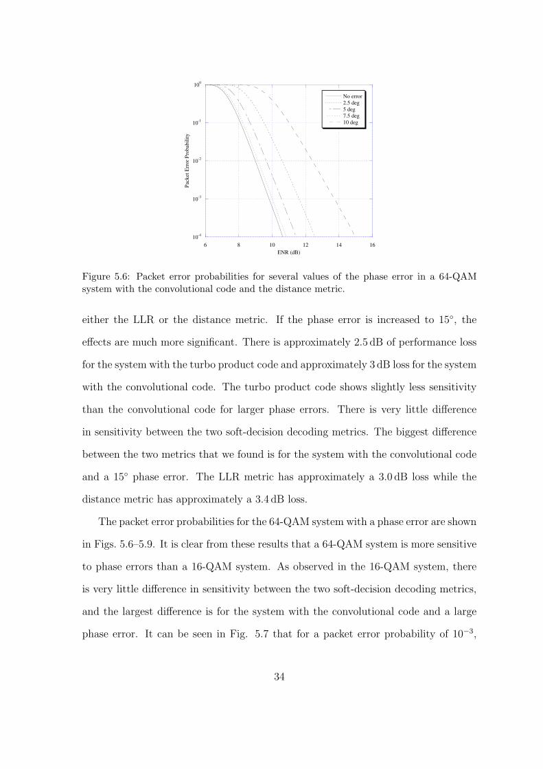
5.6 Packet error probabilities for several values of the phase errorin a 64-QAM system with the convolutional code and thedistance metric. . . . . . . . . . . . . . . . . . . . . . . . . . . . . . 34

List of Figures (Continued)

Figure Page

5.7 Packet error probabilities for several values of the phase errorin a 64-QAM system with the convolutional code and the LLRmetric. . . . . . . . . . . . . . . . . . . . . . . . . . . . . . . . . . . 35

5.8 Packet error probabilities for several values of the phase errorin a 64-QAM system with the turbo product code and thedistance metric. . . . . . . . . . . . . . . . . . . . . . . . . . . . . . 35

5.9 Packet error probabilities for several values of the phase errorin a 64-QAM system with the turbo product code and theLLR metric. . . . . . . . . . . . . . . . . . . . . . . . . . . . . . . . 36

5.10 Required ENR to achieve a 10−2 packet error probability asa function of the gain factor. . . . . . . . . . . . . . . . . . . . . . . 37

5.11 Packet error probabilities for several values of β in a 16-QAMsystem with the convolutional code and the distance metric. . . . . . 38

5.12 Packet error probabilities for several values of β in a 16-QAMsystem with the convolutional code and the LLR metric. . . . . . . . 39

5.13 Packet error probabilities for several values of β in a 64-QAMsystem with the convolutional code and the distance metric. . . . . . 39

5.14 Packet error probabilities for several values of β in a 64-QAMsystem with the convolutional code and the LLR metric. . . . . . . . 40

5.15 Packet error probabilities for several values of β in a 16-QAMsystem with the turbo product code and the distance metric. . . . . 41

5.16 Packet error probabilities for several values of β in a 16-QAMsystem with the turbo product code and the LLR metric. . . . . . . 41

5.17 Packet error probabilities for several values of β in a 64-QAMsystem with the turbo product code and the distance metric. . . . . 42

5.18 Packet error probabilities for several values of β in a 64-QAMsystem with the turbo product code and the LLR metric. . . . . . . 42

5.19 Packet error probabilities for a 64-QAM system with phaseand amplitude errors using the convolutional code. . . . . . . . . . . 43

ix

List of Figures (Continued)

Figure Page

5.20 Packet error probabilities for a 64-QAM system with phaseand amplitude errors using the turbo product code. . . . . . . . . . 43

x

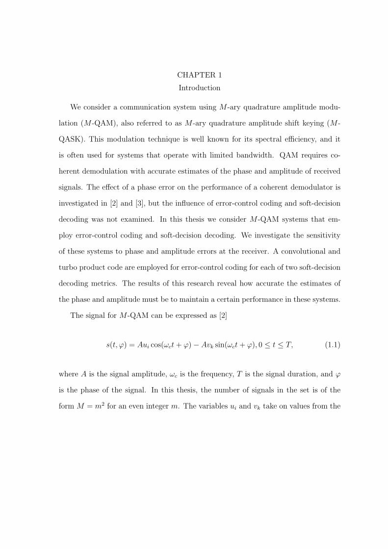
CHAPTER 1

Introduction

We consider a communication system using M -ary quadrature amplitude modu-

lation (M -QAM), also referred to as M -ary quadrature amplitude shift keying (M -

QASK). This modulation technique is well known for its spectral efficiency, and it

is often used for systems that operate with limited bandwidth. QAM requires co-

herent demodulation with accurate estimates of the phase and amplitude of received

signals. The effect of a phase error on the performance of a coherent demodulator is

investigated in [2] and [3], but the influence of error-control coding and soft-decision

decoding was not examined. In this thesis we consider M -QAM systems that em-

ploy error-control coding and soft-decision decoding. We investigate the sensitivity

of these systems to phase and amplitude errors at the receiver. A convolutional and

turbo product code are employed for error-control coding for each of two soft-decision

decoding metrics. The results of this research reveal how accurate the estimates of

the phase and amplitude must be to maintain a certain performance in these systems.

The signal for M -QAM can be expressed as [2]

s(t, ϕ) = Aui cos(ωct + ϕ)− Avk sin(ωct + ϕ), 0 ≤ t ≤ T, (1.1)

where A is the signal amplitude, ωc is the frequency, T is the signal duration, and ϕ

is the phase of the signal. In this thesis, the number of signals in the set is of the

form M = m2 for an even integer m. The variables ui and vk take on values from the

set {±1,±3, . . . ,±(m − 1)} [4]. If M = 2q, q is an even integer, and n = q/2, then

a regular M -QAM signal constellation consists of a square grid of uniformly spaced

symbols in a 2n by 2n square array. Symbols in this type of constellation are called

nearest neighbors if they are two adjacent symbols in the same row or column. A

Gray code is a one-to-one assignment of binary words of length q to the symbols in a

QAM constellation with the property that assignments for nearest neighbors disagree

in exactly one bit position. There are many Gray codes for a given constellation, but

we use the IEEE Standard Gray code for 16-QAM and 64-QAM [5]. The resulting

constellations and bit assignments are referred to as standard 16-QAM and standard

64-QAM.

All results presented in this thesis are for an additive white Gaussian noise (AWGN)

channel. A signal is sent over an AWGN channel and demodulated with a coherent

inphase-quadrature correlation receiver. The outputs of the integrators in the re-

ceiver produce the decision statistic Z = (Z1, Z2), where Z1 and Z2 are independent

Gaussian random variables. If Z1 = z1 and Z2 = z2, then we say the received point

is r = (z1, z2). The correlators require perfect knowledge of the phase and amplitude

of the received signals in order to use the maximum-likelihood decision regions. In

practice, however, the receiver’s estimates of the phase and amplitude are not per-

fectly accurate, and errors in these estimates degrade the performance of the system.

In this thesis, we investigate the level of performance degradation caused by these

types of errors.

2

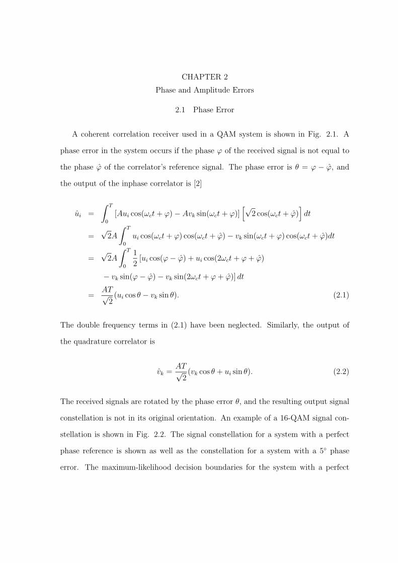
CHAPTER 2

Phase and Amplitude Errors

2.1 Phase Error

A coherent correlation receiver used in a QAM system is shown in Fig. 2.1. A

phase error in the system occurs if the phase ϕ of the received signal is not equal to

the phase ϕ of the correlator’s reference signal. The phase error is θ = ϕ − ϕ, and

the output of the inphase correlator is [2]

ui =

∫ T

0

[Aui cos(ωct + ϕ)− Avk sin(ωct + ϕ)][√

2 cos(ωct + ϕ)]dt

=√

2A

∫ T

0

ui cos(ωct + ϕ) cos(ωct + ϕ)− vk sin(ωct + ϕ) cos(ωct + ϕ)dt

=√

2A

∫ T

0

1

2[ui cos(ϕ− ϕ) + ui cos(2ωct + ϕ + ϕ)

− vk sin(ϕ− ϕ)− vk sin(2ωct + ϕ + ϕ)] dt

=AT√

2(ui cos θ − vk sin θ). (2.1)

The double frequency terms in (2.1) have been neglected. Similarly, the output of

the quadrature correlator is

vk =AT√

2(vk cos θ + ui sin θ). (2.2)

The received signals are rotated by the phase error θ, and the resulting output signal

constellation is not in its original orientation. An example of a 16-QAM signal con-

stellation is shown in Fig. 2.2. The signal constellation for a system with a perfect

phase reference is shown as well as the constellation for a system with a 5◦ phase

error. The maximum-likelihood decision boundaries for the system with a perfect

Y(t)

∫0T Z1

Z2∫0

T

Decision Device√2 α(t) cos(ωct+ϕ)

−√2 α(t) sin(ωct+ϕ)^

^

Figure 2.1: Inphase-quadrature coherent correlation receiver used for QAM demodulation.

signal constellation with no phase errorsignal constellation with 5 degree phase errormaximum likelihood decision boundaries for a system with no phase error

Figure 2.2: 16-QAM signal constellation and decision boundaries for a system with no phaseerror and a constellation with a 5◦ phase error.

phase reference are included. Each point in the rotated constellation is closer to at

least one boundary, which causes an increase of incorrect bit decisions.

The effects of phase errors on QAM systems with no error-control coding have been

investigated in [3] and [4]. The rotation of the received signals causes degradation in

the performance of the system. An expression for the average symbol error probability

for an M -QAM system with a phase error is presented in [3] and [4]. The average

4

symbol error probability as a function of θ is given by

PE(θ) =4

M

∑j

∑

l

Q{∆ [l + (1− l) cos θ − j sin θ]}

− 4

M

∑

k

∑

l

Q{∆ [k + (1− k) cos θ + (l − 1) sin θ]} ×

Q{∆ [l + (1− l) cos θ − (k − 1) sin θ]}, (2.3)

where Q(x) =∫∞

x(1/√

2π) exp (−y2/2)dy, and ∆ is related to the signal-to-noise ratio

in [4]. For 16-QAM, ∆ =√

4Eb/5N0, and for 64-QAM, ∆ =√

2Eb/7N0, where Eb/N0

is the bit-energy-to-noise density ratio. The sums over j and l are for the values

j = ±1,±3, . . . ,±(m− 1) and l = ±2,±4, . . . ,±(m− 1). The sums over k and l are

for the values k, l = 0,±2,±4, . . . ,±(m− 2). Because of the symmetry in these sets

and the behavior of the sine and cosine functions, the expression is symmetric about

θ = 0. Substituting −θ into (2.3) gives

PE(θ) =4

M

∑j

∑

l

Q{∆ [l + (1− l) cos θ + j sin θ]}

− 4

M

∑

k

∑

l

Q{∆ [k + (1− k) cos θ − (l − 1) sin θ]} ×

Q{∆ [l + (1− l) cos θ + (k − 1) sin θ]}. (2.4)

Because the set of values for the variable j contains both the positive and negative

values of each integer, the first double summation in this expression is equal to the

first double summation in (2.3). Also, because k and l take on the same values, the

second double summation in this expression is equal to the second double summation

in (2.3). Thus, the two equations are equal, and the same symbol error probability is

achieved for a phase error of θ or −θ.

As the phase error is increased, the required signal-to-noise ratio to reach a given

5

symbol error probability is also increased. Table 2.1 shows the required bit-energy-to-

noise density ratio to achieve a symbol error probability of 10−5 in a 16-QAM system

with no error control coding [3], [4]. As the phase error is increased, the required

value of ENR = 10 log10 (Eb/N0) also increases.

Table 2.1: Required ENR for a symbol error probability of 10−5 in a 16-QAM system.

Phase (deg) Required ENR (dB)0.0 14.022.5 14.725.0 16.137.5 17.9310.0 20.31

6

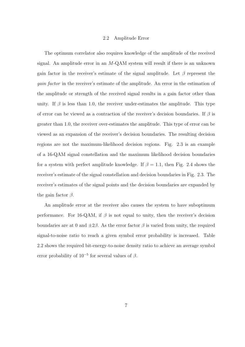
2.2 Amplitude Error

The optimum correlator also requires knowledge of the amplitude of the received

signal. An amplitude error in an M -QAM system will result if there is an unknown

gain factor in the receiver’s estimate of the signal amplitude. Let β represent the

gain factor in the receiver’s estimate of the amplitude. An error in the estimation of

the amplitude or strength of the received signal results in a gain factor other than

unity. If β is less than 1.0, the receiver under-estimates the amplitude. This type

of error can be viewed as a contraction of the receiver’s decision boundaries. If β is

greater than 1.0, the receiver over-estimates the amplitude. This type of error can be

viewed as an expansion of the receiver’s decision boundaries. The resulting decision

regions are not the maximum-likelihood decision regions. Fig. 2.3 is an example

of a 16-QAM signal constellation and the maximum likelihood decision boundaries

for a system with perfect amplitude knowledge. If β = 1.1, then Fig. 2.4 shows the

receiver’s estimate of the signal constellation and decision boundaries in Fig. 2.3. The

receiver’s estimates of the signal points and the decision boundaries are expanded by

the gain factor β.

An amplitude error at the receiver also causes the system to have suboptimum

performance. For 16-QAM, if β is not equal to unity, then the receiver’s decision

boundaries are at 0 and ±2β. As the error factor β is varied from unity, the required

signal-to-noise ratio to reach a given symbol error probability is increased. Table

2.2 shows the required bit-energy-to-noise density ratio to achieve an average symbol

error probability of 10−5 for several values of β.

7

signal constellationmaximum likelihood decision boundaries

Figure 2.3: 16-QAM signal constellation and maximum likelihood decision boundaries.

signal constellationreceiver's estimate of signal constellationmaximum likelihood decision boundariesreceiver's estimate of decision boundaries

Figure 2.4: Receiver’s estimate of a 16-QAM signal constellation and decision boundariesfor a system with β = 1.1.

8

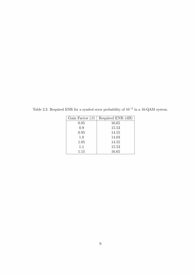
Table 2.2: Required ENR for a symbol error probability of 10−5 in a 16-QAM system.

Gain Factor (β) Required ENR (dB)0.85 16.650.9 15.530.95 14.551.0 14.031.05 14.551.1 15.531.15 16.65

9

CHAPTER 3

Log Likelihood Ratio Metric

One of the soft-decision metrics considered for decoding the received signals is a

bit metric that uses the log likelihood ratio for each of the bit positions. The value

of the ratio is used to decide what bits were sent and to place a quantitative measure

of reliability on the bit decisions. The specifications of the metric depend on the

Gray code being used in the system. For standard 16-QAM and 64-QAM, half of the

bits depend on the horizontal component of the received point, z1, and the other half

depend on the vertical component, z2. For 16-QAM, the set of coordinates used for

the symbols in the output constellation are from the set {−3,−1, +1, +3}. These are

the mean values of each coordinate of the vector decision statistic Z = (Z1, Z2) at the

output of the receiver. The log likelihood ratios for each bit decision can be written

in terms of two functions g1 and g2 [1] that are defined by

g1(z) =exp {−(z + 3)2/2σ2}+ exp {−(z + 1)2/2σ2}exp {−(z − 3)2/2σ2}+ exp {−(z − 1)2/2σ2} (3.1)

and

g2(z) =exp {−(z + 3)2/2σ2}+ exp {−(z − 3)2/2σ2}exp {−(z + 1)2/2σ2}+ exp {−(z − 1)2/2σ2} . (3.2)

For 16-QAM, the noise variance, σ2, is given by [1]

σ2 =5N0

Es

=5

4r

N0

Eb

, (3.3)

where r is the code rate of the error-control code, Es is the average energy per QAM

symbol, and Eb is the average energy per information bit. The four log likelihood ratios

are L1(r) = ln [g1(z1)], L2(r) = ln [g2(z1)], L3(r) = ln [g1(z2)], and L4(r) = ln [g2(z2)],

where Li is used for the ith bit decision. These four ratios make up the log likelihood

ratio (LLR) metric for 16-QAM.

The same concept can be applied to standard 64-QAM. The coordinates for the

symbols in the 64-QAM signal constellation are taken from the set {−7,−5,−3,−1,

+ 1, +3, +5, +7}, and the log likelihood ratios can be written in terms of three func-

tions g1, g2, and g3 that are defined by

g1(z) =exp

{−(z+7)2

2σ2

}+ exp

{−(z+5)2

2σ2

}+ exp

{−(z+3)2

2σ2

}+ exp

{−(z+1)2

2σ2

}

exp{−(z−7)2

2σ2

}+ exp

{−(z−5)2

2σ2

}+ exp

{−(z−3)2

2σ2

}+ exp

{−(z−1)2

2σ2

} , (3.4)

g2(z) =exp

{−(z+7)2

2σ2

}+ exp

{−(z+5)2

2σ2

}+ exp

{−(z−5)2

2σ2

}+ exp

{−(z−7)2

2σ2

}

exp{−(z+3)2

2σ2

}+ exp

{−(z+1)2

2σ2

}+ exp

{−(z−1)2

2σ2

}+ exp

{−(z−3)2

2σ2

} , (3.5)

and

g3(z) =exp

{−(z+7)2

2σ2

}+ exp

{−(z+1)2

2σ2

}+ exp

{−(z−1)2

2σ2

}+ exp

{−(z−7)2

2σ2

}

exp{−(z+5)2

2σ2

}+ exp

{−(z+3)2

2σ2

}+ exp

{−(z−3)2

2σ2

}+ exp

{−(z−5)2

2σ2

} . (3.6)

In this case, σ2 is given by

σ2 =21N0

Es

=7

2r

N0

Eb

. (3.7)

The six LLRs are L1(r) = ln [g1(z1)], L2(r) = ln [g2(z1)], L3(r) = ln [g3(z1)], L4(r) =

ln [g1(z2)], L5(r) = ln [g2(z2)], and L6(r) = ln [g3(z2)]. These metrics are used to make

bit decisions and provide a measure of reliability for the bit decisions that can be used

in soft-decision decoding.

3.1 Mathematical Analysis of a Phase Error

The LLR metric depends on the distances between the received point and the

inphase and quadrature components of the signal constellation points. A phase error

11

in the system causes these distances to change. The LLR metrics depend on the

fact that the x and y values of the signal constellation points come from the set

{±1,±3, . . . ,±(m−1)}. In the event of a phase error, the rotated signal constellation

points do not take on values from this set. However, there are straight lines connecting

the rotated signal points. Equations for these lines can be determined using a simple

point-slope method. These equations are in terms of the phase error θ, and can be

used to replace the signal components in the LLR metrics. Applying this method to

L1(r) results in the exponents of (3.1) taking on the form

l1(r, θ) =−(z1 − z2 tan θ + 3

√2 tan θ sin(3π

4− θ)− 3

√2 cos(3π

4− θ))2

2σ2, (3.8)

l2(r, θ) =−(z1 − z2 tan θ +

√2 tan θ sin(3π

4− θ)−√2 cos(3π

4− θ))2

2σ2, (3.9)

l3(r, θ) =−(z1 − z2 tan θ + 3

√2 tan θ sin(π

4− θ)− 3

√2 cos(π

4− θ))2

2σ2, (3.10)

and

l4(r, θ) =−(z1 − z2 tan θ +

√2 tan θ sin(π

4− θ)−√2 cos(π

4− θ))2

2σ2. (3.11)

For a phase error θ, the LLR metric for the first bit is

L1(r, θ) = ln

[exp {l1(r, θ)}+ exp {l2(r, θ)}exp {l3(r, θ)}+ exp {l4(r, θ)}

]. (3.12)

The other metrics have similar forms that depend on z1, z2, and θ. These metrics are

not symmetric about θ for a given received point; however, because of the symmetry

of the regular QAM constellation, the average effects of a phase error on a system

using the LLR metric are symmetric. For example, a phase error θ has opposite effects

12

on the first bit metric for mirrored symbols across the x-axis. So in the absence of

noise, L1((z1, z2), θ) = L1((z1,−z2),−θ). This is also true for the second bit metric,

L2. Similarly, a phase error has opposite effects on the third and fourth bit metrics for

mirrored symbols across the y-axis. Thus, in the absence of noise, L3((z1, z2), θ) =

L3((−z1, z2),−θ) and L4((z1, z2), θ) = L4((−z1, z2),−θ). This symmetry results in

the same performance for a system using the LLR metric with a phase error of θ or

−θ.

The sensitivity of the LLR to phase errors can be investigated by determining

the slopes of the lines tangent to the metric functions with respect to the variable θ.

Differentiating the metrics with respect to θ shows the level of sensitivity to changes

in phase. A phase error in any practical communication system is a small value, so the

slope of interest is the slope at θ = 0. Evaluating the derivatives at θ = 0 provides a

quantitative measure of sensitivity that can be used for comparison to other metrics.

The derivatives were evaluated for 16-QAM using eight possible received points.

These points lie on a circle centered at the signal constellation point (1,1). They are

spaced π/4 radians apart with a radius equal to one standard deviation of the noise

in the system. Most received points fall within one standard deviation of the noise,

so the majority of received points lie within this circle of test points. A depiction of

these possible received points is shown in Fig. 3.1. A 4-QAM signal constellation is

shown, but the received points can be placed around any symbol in a constellation

of any size. Using these values for z1 and z2 and θ = 0, eight slopes of the LLR

metrics were calculated. The magnitudes of these slopes were then averaged to find

the average magnitude of the slope at a phase error of zero. Table 3.1 shows the

evaluated derivatives at the 8 possible received points. The results are shown for a

bit-energy-to-noise density ratio of 2.0 dB.

If the received points lie near a corner point or other exterior point rather than an

13

signal constellation pointspossible received points

Figure 3.1: Possible received points near a QAM output signal.

Table 3.1: Slopes of LLR metrics for 16-QAM with zero phase error.

z1 z2 L′1(0) L′2(0) L′3(0) L′4(0)1.8881 1.8881 3.5233 -2.5887 -3.5233 2.5887

1 2.2559 .5509 -3.3014 -2.0096 1.33590.1119 1.8881 2.7481 -0.6682 -0.2088 0.1534-0.2559 1 1.4618 0.757 0.4029 -0.37460.1119 0.1119 0.1629 -0.0396 -0.1629 0.0396

1 -0.2559 -0.4029 0.3746 -1.4618 -0.7571.8881 0.1119 0.2088 -0.1534 -2.7481 0.66822.2559 1 2.0096 -1.3359 -3.5509 3.3014Average (magnitude) 1.7585 1.1523 1.7585 1.1523

interior point, the magnitudes of the slopes are larger. The distance from the origin

is proportional to the distance that a point moves due to a phase shift. Given a fixed

value of θ, a received point near the corner point (3,3) moves a greater distance than a

received point near the interior point (1,1). Table 3.2 displays the average magnitudes

of slopes using received points near three different symbols, each of which is a different

distance from the origin. The values in the table are for a bit-energy-to-noise density

ratio of 2.0 dB.

As the signal-to-noise ratio increases, the magnitudes of the slopes of the tangent

14

Table 3.2: Average slope magnitudes of LLR metrics for 16-QAM with zero phase error.

type (x,y) for symbol Avg |L′1(0)| Avg |L′2(0)| Avg |L′3(0)| Avg |L′4(0)|interior (1,1) 1.7585 1.1523 1.7585 1.1523

other ext. (3,1) 2.3403 1.3958 4.9734 3.1761corner (3,3) 6.5872 3.9387 6.5872 3.9387

lines increase as well. This is due to the fact that the LLR metrics depend on the

noise variance σ2. As the signal-to-noise ratio increases, the output values for the LLR

metrics increase in magnitude. A higher signal-to-noise ratio results in bit decisions

with higher reliability. An increase in the magnitude of the slope suggests an increase

in sensitivity to phase errors; however, the performance analysis of a coded system

using the LLR metric does not reflect an increase in sensitivity to phase errors as

the signal-to-noise ratio increases. So some type of normalization should be used

to account for the increase in magnitude as the signal-to-noise ratio increases. One

technique is to normalize the slope values by the magnitudes of the LLR metrics.

In Tables 3.1 and 3.2, the derivatives of the metrics were evaluated at points near

the symbol at (1,1). The signal constellation point (1,1) is also the mean value of

the random decision statistic Z, so z1 = 1 and z2 = 1 can be considered the most

likely values for the variables z1 and z2 in the LLR metric functions. Dividing the

slopes by the magnitudes of these functions at (z1, z2) = (1, 1) and θ = 0 normalizes

the effects of the signal-to-noise ratio. Table 3.3 shows the average slope magnitudes

for the interior point (1,1) in a 16-QAM system with zero phase error, and Table

3.4 shows these slopes normalized by the magnitudes of the LLR function values at

(z1, z2) = (1, 1). This same normalization technique was applied to the analysis of

a corner point and other exterior point to give the normalized magnitudes in Tables

3.5 and 3.6.

15

Table 3.3: LLR slope magnitudes for an interior point in a 16-QAM system with zero phaseerror.

ENR (dB) |L′1(0)| |L′2(0)| |L′3(0)| |L′4(0)|2 1.7585 1.1523 1.7585 1.15233 2.0489 1.4545 2.0489 1.45454 2.4043 1.7974 2.4043 1.79745 2.9065 2.5094 2.9065 2.50946 3.5171 3.3364 3.5171 3.33647 4.2672 4.2171 4.2672 4.21718 5.2133 5.2055 5.2133 5.20559 6.4373 6.4367 6.4373 6.436710 8.03 8.03 8.03 8.03

Table 3.4: Normalized LLR slope magnitudes for an interior point in a 16-QAM systemwith zero phase error.

ENR (dB) norm |L′1(0)| norm |L′2(0)| norm |L′3(0)| norm |L′4(0)|2 1.1772 0.7714 1.1772 0.77143 1.1560 0.8206 1.1560 0.82064 1.1273 0.8427 1.1273 0.84275 1.1153 0.9629 1.1153 0.96296 1.0905 1.0344 1.0905 1.03447 1.0595 1.0471 1.0595 1.04718 1.0315 1.0300 1.0315 1.03009 1.0127 1.0126 1.0127 1.012610 1.0037 1.0037 1.0037 1.0037

The normalized slope values for 16-QAM suggest that metrics for corner points

and other exterior points are more sensitive to phase errors than metrics for interior

points. Also for corner points and other exterior points, some bit decisions are more

sensitive to phase errors than others. Though the derivative analysis does not give a

conclusive result on the sensitivity of the LLR to phase errors, it does provide some

insight into the behavior of the LLR in an M -QAM system with a phase error.

16

Table 3.5: Normalized LLR slope magnitudes for a corner point in a 16-QAM system withzero phase error.


Table 3.6: Normalized LLR slope magnitudes for an other exterior point in a 16-QAMsystem with zero phase error.


3.2 Mathematical Analysis of an Amplitude Error

An amplitude error in an M -QAM system causes the distances used in the LLR

metrics to change. If there is an amplitude error, then the receiver over-estimates

or under-estimates the amplitude of the received signals, which leads to the val-

ues in the metrics being from the set {±β,±3β, . . . ,±(m − 1)β} instead of the set

{±1,±3, . . . ,±(m− 1)}. The LLR metrics for a 16-QAM system with an amplitude

17

error are

L1(r, β) = ln

[exp {−(z1 + 3β)2/2σ2}+ exp {−(z1 + β)2/2σ2}exp {−(z1 − 3β)2/2σ2}+ exp {−(z1 − β)2/2σ2}

], (3.13)

L2(r, β) = ln

[exp {−(z1 + 3β)2/2σ2}+ exp {−(z1 − 3β)2/2σ2}exp {−(z1 + β)2/2σ2}+ exp {−(z1 − β)2/2σ2}

], (3.14)

L3(r, β) = ln

[exp {−(z2 + 3β)2/2σ2}+ exp {−(z2 + β)2/2σ2}exp {−(z2 − 3β)2/2σ2}+ exp {−(z2 − β)2/2σ2}

], (3.15)

and

L4(r, β) = ln

[exp {−(z2 + 3β)2/2σ2}+ exp {−(z2 − 3β)2/2σ2}exp {−(z2 + β)2/2σ2}+ exp {−(z2 − β)2/2σ2}

]. (3.16)

The sensitivity of the LLR metric to amplitude errors can be investigated by

determining the slope of the functions in (3.13)–(3.16) with respect to the variable

β. For an amplitude error, the slope of interest is the slope at β = 1. The same type

of analysis that is described in Section 3.1 was performed for an amplitude error.

The derivatives were evaluated using eight possible received points lying on a circle

centered at the signal constellation point (1,1). Using these values for z1 and z2 and

β = 1, eight slopes of the LLR metrics were calculated. The magnitudes of these

slopes were then averaged to find the average magnitude of the slope at β = 1. Table

3.7 shows the evaluated derivatives at the eight received points using a bit-energy-to-

noise density ratio of 2.0 dB.

The magnitudes of the slopes again have a strong dependence on the signal-to-

noise ratio. As seen in Table 3.8, larger values of Eb/N0 result in larger magnitudes

for the slopes of the LLR metrics. The same method described in Section 3.1 for

normalizing the effects of the signal-to-noise ratio is employed, and the results for an

interior point are shown in Table 3.9.

18

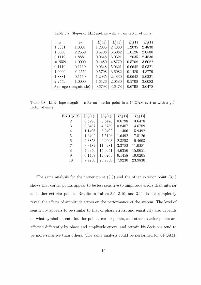
Table 3.7: Slopes of LLR metrics with a gain factor of unity.

z1 z2 L′1(1) L′2(1) L′3(1) L′4(1)1.8881 1.8881 1.2035 2.4830 1.2035 2.48301.0000 2.2559 0.5708 3.6082 1.6126 2.05800.1119 1.8881 0.0648 5.0321 1.2035 2.4830-0.2559 1.0000 -0.1480 4.8779 0.5708 3.60820.1119 0.1119 0.0648 5.0321 0.0648 5.03211.0000 -0.2559 0.5708 3.6082 -0.1480 4.87791.8881 0.1119 1.2035 2.4830 0.0648 5.03212.2559 1.0000 1.6126 2.0580 0.5708 3.6082Average (magnitude) 0.6798 3.6478 0.6798 3.6478

Table 3.8: LLR slope magnitudes for an interior point in a 16-QAM system with a gainfactor of unity.

ENR (dB) |L′1(1)| |L′2(1)| |L′3(1)| |L′4(1)|2 0.6798 3.6478 0.6798 3.64783 0.8487 4.6789 0.8487 4.67894 1.1406 5.9492 1.1406 5.94925 1.6492 7.5126 1.6492 7.51266 2.3853 9.4603 2.3853 9.46037 3.3782 11.9281 3.3782 11.92818 4.6356 15.0651 4.6356 15.06519 6.1458 19.0205 6.1458 19.020510 7.9230 23.9830 7.9230 23.9830

The same analysis for the corner point (3,3) and the other exterior point (3,1)

shows that corner points appear to be less sensitive to amplitude errors than interior

and other exterior points. Results in Tables 3.9, 3.10, and 3.11 do not completely

reveal the effects of amplitude errors on the performance of the system. The level of

sensitivity appears to be similar to that of phase errors, and sensitivity also depends

on what symbol is sent. Interior points, corner points, and other exterior points are

affected differently by phase and amplitude errors, and certain bit decisions tend to

be more sensitive than others. The same analysis could be performed for 64-QAM;

19

Table 3.9: Normalized LLR slope magnitudes for an interior point in a 16-QAM systemwith a gain factor of unity.


Table 3.10: Normalized LLR slope magnitudes for a corner point in a 16-QAM system witha gain factor of unity.


however, because of the inconclusive results of the mathematical analysis, simulations

are used for the investigation of 64-QAM.

20

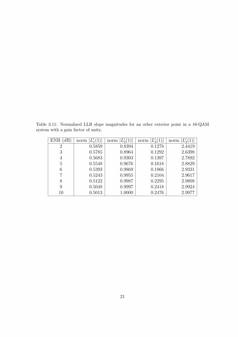
Table 3.11: Normalized LLR slope magnitudes for an other exterior point in a 16-QAMsystem with a gain factor of unity.


21

CHAPTER 4

Distance Metric

Another soft-decision metric considered for decoding received signals is referred

to as the distance metric [1]. This bit metric compares the distances from a received

point to the nearest symbols in the output constellation in order to make bit decisions.

If r = (z1, z2) is the received point, then the symbol s0 is the symbol in the output

constellation that is closest to the received point r. The bits assigned to symbol s0 are

the bit decisions. The distance from the received point to the symbol s0 is denoted

by d0. Now consider all symbols such that the ith bit differs from the ith bit of s0.

Of these symbols, the closest to the received point is denoted by si, and let di be the

distance from the received point to the symbol si. If di is much greater than d0, then

the received point is far away from any symbols that differ from s0 in the ith bit. So

the reliability for the ith bit decision should be high if di − d0 is large. Thus, the

reliability measure for each bit decision is di − d0, and these functions make up the

distance metric. Because each symbol has different neighbors, the bit metrics will be

different depending on where the received point falls. For 16-QAM, if the received

point falls closest to the symbol at the interior point (1,1), then the distances used

for the distance metric are

d0(r) =√

(z1 − 1)2 + (z2 − 1)2, (4.1)

d1(r) =√

(z1 + 1)2 + (z2 − 1)2, (4.2)

d2(r) =√

(z1 − 3)2 + (z2 − 1)2, (4.3)

d3(r) =√

(z1 − 1)2 + (z2 + 1)2, (4.4)

and

d4(r) =√

(z1 − 1)2 + (z2 − 3)2. (4.5)

The metrics used for bit decisions are D1(r) = d1−d0, D2(r) = d2−d0, D3(r) = d3−d0,

and D4(r) = d4−d0. The symbols used for these distances are all nearest neighbors of

the symbol at (1,1); however, this is not always the case. For example, if the received

point falls closest to the corner point (3,3), then there are no nearest neighbors that

differ in the first or third bits, so symbols that lie beyond nearest neighbors must be

used for these bit decisions. If the distance metric is applied to 64-QAM, there are

always bit decisions that require the use of symbols beyond nearest neighbors.

4.1 Mathematical Analysis of a Phase Error

Recall that a phase error rotates the received signal constellation points by an

angle θ. The distance metric depends on the distances from the received point to

the signal constellation points, so rotating these signals will cause these distances to

change. A QAM signal constellation occupies a two dimensional space and can be

represented by points in the complex plane. For example, the signal at the point

(1,1) can be represented by the complex value 1 + j or√

2 exp (jπ/4). Given a phase

error, θ, the angle θ is added to the phase of this signal point, and the signal becomes√

2 exp (jπ/4 + θ). The distances for the distance metric can then be viewed as the

magnitudes of vectors connecting a complex received point r = z1 + jz2 and rotated

versions of the signal constellation points. If this principle is applied to 16-QAM at

the interior point located at√

2 exp (jπ/4 + θ), then (4.1)–(4.5) become

d0(r, θ) =

√(z1 −

√2 cos(π/4 + θ))2 + (z2 −

√2 sin(π/4 + θ))2, (4.6)

23

d1(r, θ) =

√(z1 −

√2 cos(3π/4 + θ))2 + (z2 −

√2 sin(3π/4 + θ))2, (4.7)

d2(r, θ) =

√(z1 −

√10 cos(tan−1(1/3) + θ))2 + (z2 −

√10 sin(tan−1(1/3) + θ))2,

(4.8)

d3(r, θ) =

√(z1 −

√2 cos(7π/4 + θ))2 + (z2 −

√2 sin(7π/4 + θ))2, (4.9)

and

d4(r, θ) =

√(z1 −

√10 cos(tan−1(3) + θ))2 + (z2 −

√10 sin(tan−1(3) + θ))2. (4.10)

Using the argument from Section 3.1, the symmetry of the QAM constellation causes

the overall effects of a phase error on the distance metric to be symmetric. For each

symbol in the constellation, there is a mirrored symbol that has an opposing effect

for a given phase error. Thus, on average, a system with phase error θ will have the

same performance as a system with phase error −θ.

The mathematical analysis from Chapter 3 was performed to investigate the sen-

sitivity of the distance metric to phase errors. The distances in (4.6)–(4.10) are

differentiable with respect to θ. The derivatives were evaluated using eight possible

received points lying on a circle centered at (1,1) with a radius equal to one standard

deviation of the noise. Using the eight test points and θ = 0, eight slopes of the

lines tangent to the distance metrics were calculated. The magnitudes of these slopes

were then averaged to find the average magnitude of the slope at a phase error of

zero. Table 4.1 shows the evaluated derivatives at eight different received points using

a bit-energy-to-noise density ratio of 2.0 dB. Table 4.2 shows the results for several

values of Eb/N0 at this interior point.

The distance metric is not as heavily dependent on the signal-to-noise ratio as

the LLR metric. The average slope magnitudes are approximately the same for all

24

Table 4.1: Slopes of distance metrics with zero phase error.

z1 z2 D′1(0) D′

2(0) D′3(0) D′

4(0)1.8881 1.8881 3.5233 -2.5887 -3.5233 2.5887

1 2.2559 .5509 -3.3014 -2.0096 1.33590.1119 1.8881 2.7481 -0.6682 -0.2088 0.1534-0.2559 1 1.4618 0.757 0.4029 -0.37460.1119 0.1119 0.1629 -0.0396 -0.1629 0.0396

1 -0.2559 -0.4029 0.3746 -1.4618 -0.7571.8881 0.1119 0.2088 -0.1534 -2.7481 0.66822.2559 1 2.0096 -1.3359 -3.5509 3.3014Average (magnitude) 1.2553 0.896 1.2553 0.896

Table 4.2: Distance metric slope magnitudes for an interior point in a 16-QAM system withzero phase error.

ENR (dB) |D′1(0)| |D′

2(0)| |D′3(0)| |D′

4(0)|2 1.2553 0.896 1.2553 0.8963 1.253 0.9178 1.253 0.91784 1.2477 0.9351 1.2477 0.93515 1.2405 0.9488 1.2405 0.94886 1.2321 0.9596 1.2321 0.95967 1.223 0.9681 1.223 0.96818 1.2137 0.9748 1.2137 0.97489 1.2046 0.98 1.2046 0.9810 1.1958 0.9842 1.1958 0.9842

values of Eb/N0 in Table 4.2. This is also true for corner points and other exterior

points, as seen in Tables 4.3 and 4.4, so no normalization techniques are needed.

As with the LLR metric, the distance metrics that involve corner points and other

exterior points appear to be more sensitive to changes in phase than the metrics for

interior points. However, unlike the LLR metric, there appears to be little variation

among the sensitivity of different bit decisions. The slope magnitudes from Tables

4.2, 4.3, and 4.4 are often fairly close in value to the normalized slopes of the LLR

metrics in Tables 3.4, 3.5, and 3.6. This suggests that the LLR and distance metrics

25

Table 4.3: Distance metric slope magnitudes for a corner point in a 16-QAM system withzero phase error.

ENR (dB) |D′1(0)| |D′

2(0)| |D′3(0)| |D′

4(0)|2 3.4014 2.9584 3.4014 2.95843 3.3969 3.0243 3.3969 3.02434 3.3916 3.0773 3.3916 3.07735 3.3858 3.1196 3.3858 3.11966 3.38 3.1534 3.38 3.15347 3.3742 3.1805 3.3742 3.18058 3.3686 3.2023 3.3686 3.20239 3.3633 3.22 3.3633 3.2210 3.3584 3.2344 3.3584 3.2344

Table 4.4: Distance metric slope magnitudes for an other exterior point in a 16-QAM systemwith zero phase error.

ENR (dB) |D′1(0)| |D′

2(0)| |D′3(0)| |D′

4(0)|2 2.2488 1.6982 2.7518 2.6883 2.2287 1.7334 2.8072 2.75344 2.2106 1.7664 2.8499 2.80545 2.1944 1.7968 2.8823 2.84656 2.1799 1.8244 2.9067 2.87887 2.167 1.8495 2.9249 2.90438 2.1555 1.872 2.9383 2.92439 2.1452 1.8923 2.9481 2.940110 2.136 1.9104 2.9551 2.9526

have about the same level of sensitivity to phase errors. This is confirmed in the

performance analysis discussed in Chapter 5, which shows very little difference in

sensitivity to phase errors between the LLR and distance metrics. The mathematical

analysis does not provide any conclusive observations on the behavior of these metrics

in the presence of phase errors; however, it does serve as a useful tool to supplement

observations made from simulation.

26

4.2 Mathematical Analysis of an Amplitude Error

An amplitude error also affects the distance metrics. Given a gain factor β, the

receiver over-estimates or under-estimates the amplitude of the received signals such

that the values used for the distances are from the set {±β,±3β, . . . ,±(m − 1)β}.So the interior point (1,1) is assumed to be located at (β, β). Thus, (4.1)–(4.5) for

16-QAM become

d0(r, β) =√

(z1 − β)2 + (z2 − β)2, (4.11)

d1(r, β) =√

(z1 + β)2 + (z2 − β)2, (4.12)

d2(r, β) =√

(z1 − 3β)2 + (z2 − β)2, (4.13)

d3(r, β) =√

(z1 − β)2 + (z2 + β)2, (4.14)

and

d4(r, β) =√

(z1 − β)2 + (z2 − 3β)2. (4.15)

These functions can be differentiated and tested using the same method as in Section

4.1 to reveal the level of sensitivity of the distance metric to errors in amplitude.

The results for the interior point (β, β) are shown in Table 4.5 for Eb/N0 = 2.0 dB,

and Table 4.6 shows the average slope magnitudes for several values of Eb/N0. The

slope magnitudes for the distance metric again have little dependence on the signal-

to-noise ratio, but there appears to be more variation among the bit decisions than

for phase errors. The second and fourth bits appear to be more sensitive to changes

in amplitude than the first and third bits for an interior point. This is also true for

the LLR metric, as shown in Tables 3.7 and 3.9.

The average slope magnitudes for metrics that involve a corner point and other

exterior point are shown in Tables 4.7 and 4.8. For a corner point, there is little

27

Table 4.5: Slopes of distance metrics with a gain factor of unity.

z1 z2 D′1(1) D′

2(1) D′3(1) D′

4(1)1.8881 1.8881 -2.0761 -3.1342 -2.0761 -3.13421.0000 2.2559 -1.3151 -3.0088 -2.0000 -4.00000.1119 1.8881 -0.1573 -2.5736 -1.2497 -2.9682-0.2559 1.0000 0.0000 -2.0000 -0.3787 -2.07240.1119 0.1119 0.0088 -1.7472 0.0088 -1.74721.0000 -0.2559 -0.3787 -2.0724 0.0000 -2.00001.8881 0.1119 -1.2497 -2.9682 -0.1573 -2.57362.2559 1.0000 -2.0000 -4.0000 -1.3151 -3.0088Average (magnitude) 0.8982 2.6880 0.8982 2.6880

Table 4.6: Distance metric slope magnitudes for an interior point in a 16-QAM system witha gain factor of unity.

ENR (dB) |D′1(1)| |D′

2(1)| |D′3(1)| |D′

4(1)|2 0.8982 2.6880 0.8982 2.68803 0.9253 2.7534 0.9253 2.75344 0.9496 2.8054 0.9496 2.80545 0.9709 2.8465 0.9709 2.84656 0.9895 2.8788 0.9895 2.87887 1.0055 2.9043 1.0055 2.90438 1.0192 2.9243 1.0192 2.92439 1.0309 2.9401 1.0309 2.940110 1.0408 2.9526 1.0408 2.9526

variation in sensitivity among bit decisions. This differs from Table 3.10 for the

LLR metric, where the slope magnitudes of the first and third bits differ from those

of the second and fourth bits. Corner points also appear to be less sensitive to

amplitude errors than interior points for the LLR metric, but this is not the case

for the distance metric. For other exterior points, there is more variation in slope

magnitudes among different bit decisions for the LLR than for the distance metric.

In both cases, the third bit has the smallest average slope. It is difficult to determine

how these differences affect the performance of these two metrics, but simulations

28

Table 4.7: Distance metric slope magnitudes for a corner point in a 16-QAM system witha gain factor of unity.

ENR (dB) |D′1(1)| |D′

2(1)| |D′3(1)| |D′

4(1)|2 2.3761 2.1367 2.3761 2.13673 2.4256 2.1989 2.4256 2.19894 2.4694 2.2562 2.4694 2.25625 2.5081 2.3088 2.5081 2.30886 2.5425 2.3570 2.5425 2.35707 2.5728 2.4012 2.5728 2.40128 2.5996 2.4415 2.5996 2.44159 2.6234 2.4783 2.6234 2.478310 2.6444 2.5118 2.6444 2.5118

Table 4.8: Distance metric slope magnitudes for an other exterior point in a 16-QAM systemwith a gain factor of unity.

ENR (dB) |D′1(1)| |D′

2(1)| |D′3(1)| |D′

4(1)|2 2.0548 1.9788 1.0792 2.68803 2.0553 1.9974 1.1704 2.75344 2.0560 2.0120 1.2554 2.80545 2.0567 2.0232 1.3330 2.84656 2.0573 2.0318 1.4030 2.87887 2.0578 2.0384 1.4657 2.90438 2.0583 2.0435 1.5215 2.92439 2.0587 2.0474 1.5711 2.940110 2.0591 2.0504 1.6150 2.9526

show little difference in sensitivity to amplitude errors between the LLR and distance

metrics. Simulation results presented in Chapter 5, provide more insight on the effects

of phase and amplitude errors on systems using these two soft-decision decoding

metrics.

29

CHAPTER 5

Performance Analysis

5.1 Performance Results for a System with a Phase Error

To further investigate the sensitivity to phase and amplitude errors of M -QAM

systems using error-control coding and soft-decision decoding, we determine the

packet error probability for an AWGN channel. Information bits are randomly gen-

erated and encoded using two error-control coding techniques. Packets are divided

into QAM symbols and transmitted over an AWGN channel. The received signals

are demodulated with a phase error θ. Each value of θ represents the phase of the

transmitted signals, while the receiver is designed as if signals are transmitted with

a phase of zero. The received points are decoded using two soft-decision decoding

metrics. The packet error probability is shown as a function of ENR for several values

of the phase error θ. Also, the required ENR to achieve a packet error probability

of 10−2 is shown as a function of θ. The effects of a phase error were observed from

simulation results to be symmetric about zero, so results are only shown for positive

values of θ. Two error-control coding techniques are considered. A rate 1/2 convo-

lutional code with constraint length 7 is used with Viterbi decoding. The generator

polynomials for this code are (133,171) in octal. The encoder uses a packet size of

4096 binary code symbols with 2042 information bits and 6 tail bits, so the actual

code rate for the encoder is approximately 0.4985. A turbo product code of rate

0.495 [6] is also considered. This three-dimensional code is derived from two (32,26)

extended Hamming codes and a (4,3) parity-check code. This code also uses a packet

size of 4096 binary code symbols with 2028 information bits [1].

The ENR required to achieve a packet error probability of 10−2 is shown in Fig.

4

5

6

7

8

9

10

11

12

0 2 4 6 8 10 12 14 16

Requ

ired

ENR

(dB)

Phase Error (deg)

16-QAM, ConvolutionalDistance LLR

16-QAM, TPCDistance LLR



Figure 5.1: Required ENR to achieve a 10−2 packet error probability as a function of thephase error

5.1 for the different M -QAM systems considered. The biggest factor in determining

phase error sensitivity is the size of the QAM signal set. The curves for 64-QAM are

much steeper than those for 16-QAM. The phase error is varied from zero to 10◦ for

64-QAM and zero to 15◦ for 16-QAM. Given a 10◦ phase error, the 64-QAM system

requires an ENR approximately 3 dB larger than a system with no phase error. There

is very little difference in sensitivity between the two error-control coding techniques

or the soft-decision decoding metrics, although there are slight differences for large

phase errors. These subtle differences are further examined in Figs. 5.2–5.5.

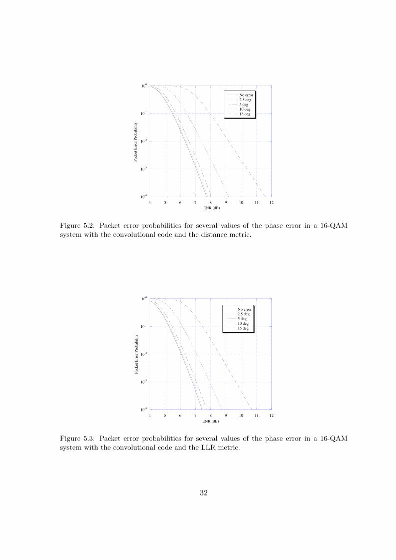
The packet error probabilities for the 16-QAM system with the convolutional code

are shown in Figs. 5.2 and 5.3. For a packet error probability of 10−3, a 16-QAM

system with the convolutional code and a 10◦ phase error requires approximately

1.2 dB higher Eb/N0 than a system with no phase error. This is true for a system

that employs either the LLR or the distance metric. The performance for a 16-QAM

system with the turbo product code is shown in Figs. 5.4 and 5.5. With a 10◦ phase

error, this system requires approximately 1.0 dB higher Eb/N0 for a system employing

31

10-4

10-3

10-2

10-1

100

4 5 6 7 8 9 10 11 12

No error2.5 deg5 deg10 deg15 deg

Pack

et E

rror P

roba

bilit

y

ENR (dB)

Figure 5.2: Packet error probabilities for several values of the phase error in a 16-QAMsystem with the convolutional code and the distance metric.

10-4

10-3

10-2

10-1

100

4 5 6 7 8 9 10 11 12


Pack

et E

rror P

roba

bilit

y

ENR (dB)

Figure 5.3: Packet error probabilities for several values of the phase error in a 16-QAMsystem with the convolutional code and the LLR metric.

32

10-4

10-3

10-2

10-1

100

3 4 5 6 7 8 9


Pack

et E

rror P

roba

bilit

y

ENR (dB)

Figure 5.4: Packet error probabilities for several values of the phase error in a 16-QAMsystem with the turbo product code and the distance metric.

10-4

10-3

10-2

10-1

100

3 4 5 6 7 8


Pack

et E

rror P

roba

bilit

y

ENR (dB)

Figure 5.5: Packet error probabilities for several values of the phase error in a 16-QAMsystem with the turbo product code and the LLR metric.

33

10-4

10-3

10-2

10-1

100

6 8 10 12 14 16

No error2.5 deg5 deg7.5 deg10 deg

Pack

et E

rror P

roba

bilit

y

ENR (dB)

Figure 5.6: Packet error probabilities for several values of the phase error in a 64-QAMsystem with the convolutional code and the distance metric.

either the LLR or the distance metric. If the phase error is increased to 15◦, the

effects are much more significant. There is approximately 2.5 dB of performance loss

for the system with the turbo product code and approximately 3 dB loss for the system

with the convolutional code. The turbo product code shows slightly less sensitivity

than the convolutional code for larger phase errors. There is very little difference

in sensitivity between the two soft-decision decoding metrics. The biggest difference

between the two metrics that we found is for the system with the convolutional code

and a 15◦ phase error. The LLR metric has approximately a 3.0 dB loss while the

distance metric has approximately a 3.4 dB loss.

The packet error probabilities for the 64-QAM system with a phase error are shown

in Figs. 5.6–5.9. It is clear from these results that a 64-QAM system is more sensitive

to phase errors than a 16-QAM system. As observed in the 16-QAM system, there

is very little difference in sensitivity between the two soft-decision decoding metrics,

and the largest difference is for the system with the convolutional code and a large

phase error. It can be seen in Fig. 5.7 that for a packet error probability of 10−3,

34

10-4

10-3

10-2

10-1

100

6 8 10 12 14 16


Pack

et E

rror P

roba

bilit

y

ENR (dB)

Figure 5.7: Packet error probabilities for several values of the phase error in a 64-QAMsystem with the convolutional code and the LLR metric.

10-4

10-3

10-2

10-1

100

6 7 8 9 10 11 12 13


Pack

et E

rror P

roba

bilit

y

ENR (dB)

Figure 5.8: Packet error probabilities for several values of the phase error in a 64-QAMsystem with the turbo product code and the distance metric.

35

10-4

10-3

10-2

10-1

100

6 7 8 9 10 11 12 13


Pack

et E

rror P

roba

bilit

y

ENR (dB)

Figure 5.9: Packet error probabilities for several values of the phase error in a 64-QAMsystem with the turbo product code and the LLR metric.

there is approximately a 3 dB loss in performance for a system with the LLR metric

and a 10◦ phase error. In Fig. 5.6, for the system with the distance metric, there

is approximately a 4 dB loss. In both the 16-QAM and 64-QAM systems with the

convolutional code and a large phase error, the LLR metric shows less performance

degradation than the distance metric.

The LLR metric outperforms the distance metric in all cases. However, the dis-

tance metric has the benefit of lower complexity, and it does not require knowledge

of the noise variance. There is little difference in sensitivity to phase errors between

the two metrics, but the LLR metric was observed to be slightly less sensitive in some

cases for large phase errors. The sensitivity also increases as the size of the QAM

signal set increases. 64-QAM is much more sensitive to phase errors than 16-QAM

for both the LLR and distance metrics and for both the convolutional and turbo

product codes. The number of signals in an M -QAM system is the primary factor in

determining the sensitivity to a phase error in the system.

36

4

5

6

7

8

9

10

11

0.8 0.85 0.9 0.95 1 1.05 1.1 1.15 1.2

Requ

ired

ENR

(dB)

Gain Factor



Distance LLR16-QAM, Convolutional


Figure 5.10: Required ENR to achieve a 10−2 packet error probability as a function of thegain factor.

5.2 Performance Results for a System with an Amplitude Error

To examine the effects of amplitude errors on the performance of QAM systems,

a gain factor of β is applied at the receiver in the performance analysis from Section

5.1. The required ENR to achieve a packet error probability of 10−2 is shown as a

function of the gain factor in Fig. 5.10. Results are included for the 16-QAM and 64-

QAM systems for the two error-control coding techniques and soft-decision decoding

metrics considered in Section 5.1.

The performance degradation caused by an amplitude error is not symmetric.

Under-estimating the amplitude at the receiver (i.e., β < 1) causes slightly worse

performance than over-estimating by the same amount(i.e., β > 1), and this can be

seen in Figs. 5.10–5.18. In Fig. 5.10, each curve is slightly higher on the left than

on the right because under-estimating the amplitude requires a higher value of ENR.

It is also clear from Fig. 5.10 that 64-QAM is much more sensitive to amplitude

errors than 16-QAM. The curves for 64-QAM are much steeper than the curves for

16-QAM, and for a gain factor of 0.85, the 64-QAM system suffers more than twice

37

10-4

10-3

10-2

10-1

100

4 5 6 7 8 9

No error0.91.10.851.150.81.2

Pack

et E

rror P

roba

bilit

y

ENR (dB)

No error

0.9

1.10.85

1.15

1.2

0.8

Figure 5.11: Packet error probabilities for several values of β in a 16-QAM system with theconvolutional code and the distance metric.

the performance loss of the 16-QAM system.

The packet error probability is shown as a function of ENR for several values of

β in Figs. 5.11–5.18. These results also show the reduced penalty of over-estimating

compared with under-estimating the amplitude. In each case, under-estimating the

amplitude results in a higher packet error probability than over-estimating by the

same amount. The LLR metric shows better performance and is also slightly less

sensitive to amplitude errors than the distance metric. However, as with phase errors,

these differences are subtle and the size of the QAM signal set is the primary factor

in sensitivity to amplitude errors. 64-QAM requires more accurate estimates of the

amplitude than 16-QAM. In Figs. 5.13 and 5.14, a gain factor of 0.85 in a 64-QAM

system requires approximately 2 dB higher ENR to achieve a packet error probability

of 10−3 versus approximately 0.5 dB for 16-QAM, as seen in Figs. 5.11 and 5.12.

There is also very little difference in sensitivity between the two error-control coding

techniques. The performance degradation due to amplitude errors in systems with

the turbo product code is about the same as the degradation in systems with the

38

10-4

10-3

10-2

10-1

100

4 5 6 7 8 9

No error0.91.10.851.150.81.2

Pack

et E

rror P

roba

bilit

y

ENR (dB)

No error

1.1

0.9

1.15

0.85

1.2

0.8

Figure 5.12: Packet error probabilities for several values of β in a 16-QAM system with theconvolutional code and the LLR metric.

10-4

10-3

10-2

10-1

100

6 7 8 9 10 11 12 13

No Error0.951.050.91.10.851.15

Pack

et E

rror P

roba

bilit

y

ENR (dB)

Figure 5.13: Packet error probabilities for several values of β in a 64-QAM system with theconvolutional code and the distance metric.

39

10-4

10-3

10-2

10-1

100

6 7 8 9 10 11 12 13

No Error0.951.050.91.10.851.15

Pack

et E

rror P

roba

bilit

y

ENR (dB)

Figure 5.14: Packet error probabilities for several values of β in a 64-QAM system with theconvolutional code and the LLR metric.

convolutional code.

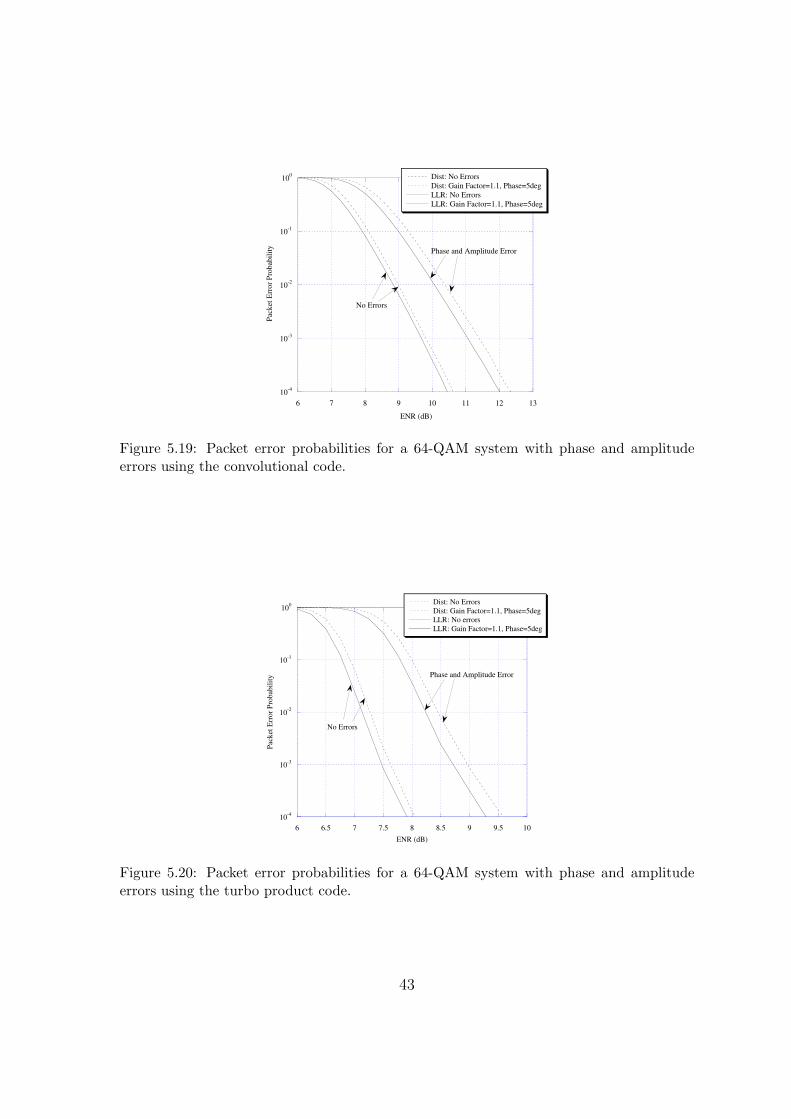
In practice, both the phase and amplitude must be estimated. Figures 5.19 and

5.20 show results for a 64-QAM system with both a 5◦ phase error and a gain factor

of 1.1. As expected, an incorrect estimate of both the phase and amplitude causes

more performance degradation than an incorrect estimate of either one alone. A 5◦

phase error or gain factor of 1.1 causes about a 0.5 dB loss in performance in a 64-

QAM system; however, the presence of both errors causes over 1 dB of performance

loss in the system for both error-control coding techniques and soft-decision decoding

metrics.

40

10-4

10-3

10-2

10-1

100

3 3.5 4 4.5 5 5.5 6

No error0.91.10.851.150.81.2

Pack

et E

rror P

roba

bilit

y

ENR (dB)

0.8

1.2

0.851.1

0.9

1.15

No error

Figure 5.15: Packet error probabilities for several values of β in a 16-QAM system with theturbo product code and the distance metric.

10-4

10-3

10-2

10-1

100

3 3.5 4 4.5 5 5.5 6

No error 0.91.10.851.150.81.2

Pack

et E

rror P

roba

bilit

y

ENR (dB)

0.8

1.2

0.85

No error

1.1

0.9

1.15

Figure 5.16: Packet error probabilities for several values of β in a 16-QAM system with theturbo product code and the LLR metric.

41

10-4

10-3

10-2

10-1

100

6 6.5 7 7.5 8 8.5 9 9.5 10

No error0.951.050.91.10.851.15

Pack

et E

rror P

roba

bilit

y

ENR (dB)

Figure 5.17: Packet error probabilities for several values of β in a 64-QAM system with theturbo product code and the distance metric.

10-4

10-3

10-2

10-1

100

6 6.5 7 7.5 8 8.5 9 9.5 10

No error 0.951.050.91.10.851.15

Pack

et E

rror P

roba

bilit

y

ENR (dB)

Figure 5.18: Packet error probabilities for several values of β in a 64-QAM system with theturbo product code and the LLR metric.

42

10-4

10-3

10-2

10-1

100

6 7 8 9 10 11 12 13

Dist: No ErrorsDist: Gain Factor=1.1, Phase=5degLLR: No ErrorsLLR: Gain Factor=1.1, Phase=5deg

Pack

et E

rror P

roba

bilit

y

ENR (dB)

No Errors

Phase and Amplitude Error

Figure 5.19: Packet error probabilities for a 64-QAM system with phase and amplitudeerrors using the convolutional code.

10-4

10-3

10-2

10-1

100

6 6.5 7 7.5 8 8.5 9 9.5 10

Dist: No ErrorsDist: Gain Factor=1.1, Phase=5degLLR: No errorsLLR: Gain Factor=1.1, Phase=5deg

Pack

et E

rror P

roba

bilit

y

ENR (dB)

No Errors

Phase and Amplitude Error

Figure 5.20: Packet error probabilities for a 64-QAM system with phase and amplitudeerrors using the turbo product code.

43

CHAPTER 6

Conclusion

Inaccurate estimates of the phase and amplitude of M -QAM signals can cause

significant degradation in the performance of the system. Although error-control

coding and soft-decision decoding can reduce the effects of phase and amplitude errors,

they do not remove them. The log likelihood ratio metric and the distance metric

have similar performance in the presence of phase and amplitude errors in an M -

QAM system. The LLR metric has a slight advantage for amplitude errors and for

large phase errors. The turbo product code has a clear advantage in performance over

the convolutional code; however, it does not show a clear advantage in performance

sensitivity to phase and amplitude errors. Both error-control coding techniques have

about the same degree of sensitivity to such errors. In general, the number of signals

in an M -QAM signal set is the primary factor in determining the required accuracy

of phase and amplitude estimates. As the size of the signal set increases, more

accurate estimates are required and thus more sophisticated techniques for estimating

these parameters are required. Under-estimating the amplitude causes slightly worse

performance than over-estimating the amplitude by the same amount. This suggests

that a positive bias might be used for the amplitude estimates of a QAM signal.

REFERENCES

[1] W. G. Phoel, J. A. Pursley, M. B. Pursley, and J. S. Skinner, “Frequency-hopspread spectrum with quadrature amplitude modulation and error-control cod-ing,” Proceedings of the 2004 IEEE Military Communications Conference (Mon-terey, CA), vol. 2, pp. 913–919, November 2004.

[2] M. B. Pursley, Introduction to Digital Communications, Upper Saddle River, NJ:Prentice Hall, 2005.

[3] M. K. Simon, S. M. Hinedi, and W. C. Lindsey, Digital Communication Tech-niques, Englewood Cliffs, NJ: PTR Prentice Hall, 1995.

[4] M. K. Simon and J. G. Smith, “Carrier synchronization and detection of QASKsignal sets,” IEEE Transactions on Communications, vol. 22, no. 2, pp. 98–106,February 1974.

[5] Institute of Electrical and Electronics Engineers, Standard 802.11-2007, Part 11: Wireless LAN Medium Access Control (MAC)and Physical Layer (PHY) Specifications, June 2007. Available:http://standards.ieee.org/getieee802/download/802.11-2007.pdf

[6] Advanced Hardware Architectures, Inc., Product Specification for AHA4501Astro 36 Mbits/sec Turbo Product Code Encoder/Decoder. Available:http://www.aha.com

effects of phase and amplitude errors on qam …

Documents