effects of landscape pattern and topography on emissions and...

Effects of Landscape Pattern and Topography onEmissions and Transport

Franz X. Meixner1 and Werner Eugster2

1Biogeochemistry Dept., Max Planck Institute for Chemistry,P.O. Box 3060, D–55020 Mainz, Germany

2Institute of Geography, University of Bern, Hallerstrasse 12, CH-3012 Bern, Switzerland

and Dept. of Plant Ecology, University of Bayreuth, D–95440 Bayreuth, Germany

This article appeared as Chapter 8 in Tenhunen and Kabat (1999)1 on pages 143–175.

Abstract

Landscape pattern (land use and natural patchiness) and complex topography strongly influence re-gional variation in emissions of trace gases and pollutants, as well as atmospheric transport processes.This leads to small-scale variation in the amount of (biogenic) emission, atmospheric deposition and inlocal concentrations of atmospheric consitutents. This chapter addresses the most important processesthat control trace gas emission and that govern atmospheric transport in nonflat and nonhomogeneouslandscapes. The focus is on the controlling factors of biogenic emissions and on those transport anddeposition processes that differ from idealized conditions in flat and homogeneous terrain.

1 Introduction

The steady increase of carbon dioxide and several other trace gases in our atmosphere will have seriousconsequences for the habitability of our planet (Ramanathan et al. 1987). Among these consequences are:

1. global warming due to increased atmospheric concentrations of greenhouse gases (e.g. CO2, CH4,N2O),

2. destruction of the stratospheric ozone layer due to increased halogenated compounds and N2O,

3. the increase of tropospheric ozone due to increased emissions of nitrogen oxides NOx (NOx = NO + NO2),CO, and volatile organic compounds (VOCs), and

4. changes in tropospheric cloud cover and stratospheric aerosol due to increased emissions of ofdimethyl sulfate (DMS) and carbonyl sulfide (COS).

While the global cycles of some of these trace gases are heavily affected by anthropogenic emissions(e.g. CO2, CO, NOx), most of them are dominated by biospheric processes (within soil, vegetation, waters,and animals). In this chapter, we focus on biogenic emissions, especially those from soils. Knowledge onhow biogenic emissions vary with landscape pattern and/or topography is scarce. Therefore, we emphasizethose emission controlling factors that may be affected most by landscape pattern and topography.

Both anthropogenic and biogenic emissions are generally nonequally distributed in complex land-scapes. Furthermore, atmospheric transport in complex landscapes also leads to regional- and small-scaledifferences in concentrations and deposition. We examine the potential effects of specific transport pro-cesses thought to have an influence at regional and local scales that result in differences between idealized(homogeneous landscape, flat terrain) and actual encountered conditions. In the case of atmospheric trans-port processes, patchy land-use pattern and complex terrain exhibit interactive effects. Therefore, we willnot separate our discussion two components and are well aware that some of our considerations also applyto patchy land-use patterns on a flat topography.

1Tenhunen, J. D. and P. Kabat (eds.), 1999. Integrating Hydrology, Ecosystem Dynamics, and Biogeochemistry in ComplexLandscapes Series Report of the Dahlem Workshop held in Berlin, January 18–23, 1998. Chichester: John Wiley & Sons Ltd., 367pp.

1

Table 1: Contribution of soils to the global cycles of atmospheric trace gases. AfterConrad (1996); Meixner (1994).

Trace Ambient Lifetime Total Annual Contribution ContributionGas Concentration (days) Budget Increase of Soils as of Soils as

(ppb) (Tg y−1) (%) Source (%) Sink (%)CO 70–170 100 2600 1.0 1 15CH4 1700 4000 540 ≈0.8 60 5COS 0.5 1500 2.3 0 23?a 23?a

N2O 310 60,000 15 0.2–0.3 70 ?NO 0.1-20 1 60 ? 20 ?DMS ≈0.1 ≈0.9 38 ? ≈0.1 0

aInferred from Andreae and Crutzen (1997); however, any contribution of soils as a source of COSis presently under discussion.

2 Emission of trace gases from soils and vegetation

Many trace gases are produced and consumed within soils. Therefore, soils can contribute to the globalbudgets of CO, CH4, COS, N2O, NO, and DMS as both sources and sinks (Table 1). The budget values andpercent contributions in Table 1 are highly uncertain for a number of reasons (Conrad 1996). With a vary-ing degree of reliability, fluxes of many trace gases can presently be measured with a variety of techniques,ranging from small (leaf) scale enclosure to tower based/airborne micrometeorological techniques, rangingfrom small-scale leaf enclosure to tower-based and airborne micrometeorological methods (Matson andHarriss 1995). Nevertheless, it is by far not trivial to estimate atmospheric budgets from fluxes measured atindividual field sites (Andreae and Schimel 1989). Most uncertainties and problems can be traced to the factthat fluxes, determined by a vast diversity in mostly microbial processes, are highly variable with respectto time and space. The problems are not necessarily solved by integration of fluxes over larger areas andlonger time periods, since “each individual flux event is caused by deterministic processes that change in anonlinear way when conditions even change slightly” (Conrad 1996). This is also valid for the variation inbiogenic emissions from plants (Table 2, especially for those of volatile organic compounds (nonmethaneVOCs). There are several hundreds of biogenic VOCs known, but those of atmospheric relevance maycomprise the isoprenoids, alkanes and alkenes, organic acids (e.g., formic and acetic acids), carbonyl com-pounds (e.g., aldehydes), alcohols, as well as esters and ethers (e.g., methanol, ethanol, ethylacetate). Theglobal source strength of the most prominent biogenic VOC compounds, isoprene and monoterpenes, isestimated to range between 300–980 Tg y−1, which is similar to and above the global source strength ofCH4 (540 Tg y−1; Table 1). The carbon loss due to biogenic VOC emissions is generally considered notto exceed some few percent of plant assimilated carbon (c.f. Kesselmeier and Staudt 1999); occasionallyit may reach some 10%–20%. However, biogenic VOC emissions comprise more than two thirds of globalVOC emissions, which play a crucial role in atmospheric chemistry, particulary for tropospheric oxidantformation, including ozone.

2.1 Mechanisms of Trace Gas Production and Consumption in Soils

Soil processes can be classified into chemical (abiotic), and microbial (biotic) processes. Additional soilenzymatic processes, which are very important for the sink strength of atmospheric hydrogen (H2), butunimportant for CO, CH4, COS, N2O, NO, and DMS, are not discussed here. Chemical processes forCOS production and consumption are likely but unknown; those for NO can either not be quantified atpresent, or their importance (e.g., NO oxidation by O2) is limited by the requirement of unrealistic high NOmixing ratios in soil air (Conrad 1996). The production of CO in soils is dominated by chemical processes,namely the thermal decomposition of humic acids and other organic material. However, the contributionof soil emissions to the global CO budget is marginal (Table 1). Microorgamisms are responsible for mostproduction and consumption processes in soils. In their oxidative and reductive metabolisms, trace gasescould act as growth substrates and/or co-metabolites, or they are considered to be stoichiometric and other

2

Table 2: Contribution of plants to the global cycles of atmospheric trace gases.Trace Ambient Lifetime Total Annual Contribution ContributionGas Concentration (days) Budget Increase of Plants as of Plants as

(ppb) (Tg y−1) (%) Source (%) Sink (%)CO a 70–170 100 2600 1.0 6 0VOCsb 0.1–100 0.004–2 900–1400 ? 80 1?COSc 0.5 1500 2.3 0 0 40d

NO e 0.1–20 1 60 ? 4 ?DMS f ≈0.1 ≈0.9 32–83 ? 5–45 0

aSeiler and Conrad (1987); Schade (1997)bKesselmeier and Staudt (1999)cKesselmeier et al. (1997)dAndreae and Crutzen (1997)eWildt et al. (1996)fAndreae and Jaeschke (1992)

products. For a comprehensive review on microorganisms and relevant metabolic mechanisms, the readeris referred to Conrad (1996). From this review, we can learn that production and consumption, and henceexchange of trace gases between soils and atmosphere, are predominantly controlled on the microscopiclevel, i.e., the level of microorganisms’ metabolism. However, in the context of how landscape pattern andtopography may affect biogenic trace gas emissions, a higher scale of organization and controls must beconsidered.

2.2 Controls of Emission Pathways from Soils by Functional Groups and Processes

Considering production and consumption of trace gases from soils, Davidson and Schimel (1995) preferso-called functional groups rather than species of microorganisms, since (a) common modes of metabolismexist among many groups of microbes and (b) knowing the predominant functional group facilitates iden-tification of factors which control rates of production and consumption. Because of limited space, weconfine the following discussion to functional groups, processes, and chemical and physical properties thatare important for CH4, N2O, and NO emissions from soils.

2.2.1 Methane Production

Methane-producing bacteria (methanogens) are a group of the archaeobacteria, which predominantely pro-duce CH4 via cleaving acetate to CO2 and CH4, and reducing CO2 with H2. Acetate (as substrate formethanogens) and H2 may originate from the fermentation of simple substrates (sugars, amino acids, etc.),which are released directly by plants or from soil organic matter breakdown. Most methanogens operatewithin a temperature range of about 20◦–40◦C and are very responsive to temperature changes within thisrange. Methanogens are extremely sensitive to oxygen and reactive oxygen species: methane productionin soils occurs under anaerobic and highly reducing conditions in the absence of NO3

−, SO42−, or ferric

ion. Therefore, rice paddies (rich in organic matter), wetlands (tropical, temperate and arctic or boreal),marine sediments, the digestive tract of many animals and insects, as well as anaerobic sewage digestors areprominent methane production sites. Significant CH4 production was also observed in (generally aerobic)upland soils as a consequence of rain events saturating the soil for a more or less extended period. How-ever, CH4 production in soils should not be confused with CH4 emission from wetland soils: more than80% of the diffusive CH4 flux from the anaerobic part of the soil is oxidized in the oxic layer of freshwaterwetlands. However, ebullition flux of CH4 (and other trace gases contained in the bubbles) from inundatedand nonvegetated wetlands does not seem to be affected by the CH4-oxidizing bacteria (Conrad 1996). Ifwetland soils are covered by appropriate vegetation, the transport through the aerenchyme of those plantsis the dominating emission pathway to the atmosphere (e.g., Davidson and Schimel 1995).

3

2.2.2 Methane Oxidation

Methane-oxidizing bacteria (methanotrophs) are a diverse group of aerobic bacteria, but they are ubiquitousand can be found in all types of soils. They oxidize CH4 primarily by (a) the enzyme CH4 monooxygenase(methanotrophic bacteria) and (b) the enzyme NH3 monooxygenase (nitrifying bacteria). O2 is requiredand is an obligate reagent in the first reaction of the oxidation pathway. Thus, any soil that is porous enoughto allow the diffusion of atmospheric O2 into it has the potential to act as a net consumer of CH4 (as it is thecase for the majority of aerated upland soils). In those ecosystems where seasonal inundation occurs (ricepaddies, tropical floodplains, arctic or boreal wetlands), the position of the water table may be the primaryfactor regulating the magnitude and even the sign of the CH4 exchange with the atmosphere.

2.2.3 Denitrification

In denitrification (an anaerobic process), bacteria utilize nitrate (NO3−) and nitrite (NO2

−) for their growthand reduce them (via N2O and NO) to N2. The absence of oxygen results from either high soil watercontent or large respiration and oxygen consumption rates in the soil. Readily oxidizable organic carbon isa requirement for most denitrifying bacteria (heterotrophs). Denitrification occurs over a wide temperaturerange (maximum rate at∼65–70◦C), roughly doubling with every 10 K increase. However, the ability ofspecific denitrifying bacteria to produce and consume N2O and NO was shown (Conrad 1996).

2.2.4 Nitrification

Nitrification involves the biological oxidation of nitrogen, typically the oxidation of soil ammonium (NH4+)

to NO3− (with NO2

− as intermediate), but there are also bacteria which oxidize NH4+ to NO2

− and NO2−

to NO3−. These bacteria are generally chemoautotrophic and require only CO2, H2O, O2, and either NH4+

or NO2− for growth. If NH4

+ or urea ((NH2)2CO) is present, nitrification will occur in well-aerated soils.As a by-product of NH4+ oxidation, nitrifying bactria produce N2O and NO. While in case of NO it isunknown which biochemical pathway is the most important for NO, the N2O production is most likelyvia reduction of NO2− by NH4

+ oxidizers. It has been shown that NO production may be dominated bynitrification in a particular soil and by denitrification in another one (Conrad 1996).

2.2.5 Bidirectional Fluxes and the Compensation-Concentration Concept

As discussed above, trace gas production and consumption processes occur simultaneously in a given(upland) soil; consequently, bidirectional fluxes have been observed under laboratory and field conditions.A conceptual explanation is given in Figure 1: the relative distribution of trace gas-producing vs. trace gas-consuming soil crumbs in upland soil determines the magnitude of corresponding (gross) fluxes from andto the surface (caveat: only net fluxes can be measured with techniques commonly applied in the field). Inaggregated soils, soil crumbs may be considered as units of trace gas metabolism (in nonaggregated soils,sand grains covered with a microbial biofilm may play that role). Soil crumbs are usually heteorogeneousregarding their aerobic–anaerobic metabolism, since even (generally well) aerated upland soils may alsocontain anoxic microniches (Conrad 1996).

The compensation-concentration concept is based on simultaneous trace gas production and consump-tion in a given bulk soil sample and on the observation that consumption rates are a function of trace gasconcentration, whereas production rates are not. The compensation concentration is then “the concentra-tion at which the consumption rate reaches the same value as the production rate so that the result of bothprocesses is zero flux” (Conrad 1994). Given the (gross) production rateP and the pseudo first-order up-take constantk of a specific trace gas, then the net release rateR is given asR = P − km (wherem isthe atmospheric trace gas concentration), and the compensation concentration is given asmc = P/k. Thenet release rate is linked to the fluxF between the soil and the atmosphere by the diffusion within the soil.This was first described by the conceptual model of Galbally and Johansson (1989) and can be formulatedasF = R/k

√(kρsD) = (mc − m)

√(kρsD), whereρs is the bulk density of the dry soil andD the

diffusivity of the trace gas in the soil. It is evident that (a) the magnitude of the fluxF increases with thedifference between the compensation and ambient concentrations, and (b)F will result in a net emission

4

F.X. Meixner and W. Eugster Figure 1——————————————————————————————————————————

——————————————————————————————————————————All rights reserved by the authors. No citing, abstracting, or other usage is permitted.

Figure 1 : Conceptual scheme of H2, CO, NO, and N2O bi-directional fluxes between upland

soil and the atmosphere as a result of the relative amount of soil entities (e.g. soil

crumbs) that either release trace gas into the soil air (solid symbols) or take it up

(open symbols). Figure taken from Conrad (1996).

Figure 1: Conceptual scheme of H2, CO, NO, and N2O bidirectional fluxes between upland soil and theatmosphere as a result of the relative amount of soil entities (e.g., soil crumbs) that either release trace gasinto the soil air (solid symbols) or take it up (open symbols). Figure taken from Conrad (1996).

from the soil ifmc > m and in a net uptake ifmc < m. Sensitivity analysis has shown thatF stronglydepends onk (Remde et al. 1993).

For the application of the compensation concept, it is essential that production and consumption pro-cesses are more or less homogeneously distributed in the soil layer (sample) under investigation. In thecase of CH4, there is obviously a substantial vertical separation of both processes in most soils; no CH4

compensation points were reported so far (Conrad 1994, 1996). Generally, the compensation concentrationmay be considered as a critical variable of the regulation of trace gas surface exchange, if (a) there is a dy-namic change of compensation concentration in the soil and/or high fluctuations of ambient concentrations,and (b) at least a partial overlap of ranges of compensation and ambient concentration must exist (see Table3). Under these premises, CO and NO are likely candidates for the compensation-concentration concept,whereas COS and N2O are usually not. For techniques and methods how to determine compensation pointconcentrations, the reader is referred to Conrad (1994).

Table 3: Overlapping and nonoverlapping ranges of am-bient and compensation concentrations. After Conrad(1994); completed by data from Meixner (1994).

Trace Gas Ambient Concentration Compensation-Concentration(ppb) (ppb)

CO 70–170 ≈5–1200COS 0.5 10–200N2O 310 ca. 500NO <0.1–20 0.3–75 (aerobic)

1600–2200 (anaerobic)

5



-5

0

5

10

15

20

1 10 100soil nitrate content [mg-N kg-1]

net N

O fl

ux

[ng-

N m

-2s-1

] Manndorf (D), wheat, reduced fertilization Manndorf (D), wheat, normal fertilizationGrote Heide (NL), heathland Halvergate Marshes (UK), pasture

Figure 2 : The net NO flux from different European ecosystems as dependent from their soil

nitrate content : Halvergate (UK) September 1989; Manndorf (D, Lower Bavaria)

May, June, July, August 1990; Grote Heide (NL) May 1991. Data are from Ludwig,

J. 1994. Untersuchungen zum Austausch von Stickoxiden zwischen Biosphäre und

Atmosphäre. PhD Thesis. University of Bayreuth, Bayreuth, Germany.

Figure 2: The net NO flux from different European ecosystems as a function of soil nitrate content: Halver-gate (UK) September 1989; Manndorf (D, Lower Bavaria) May, June, July, August 1990; Grote Heide (NL)May 1991. Data are from Ludwig (1994).

2.2.6 Nitrogen Availability

Considering the microbial processes which determine the production and consumption of CO, CH4, N2O,and NO in soils, it becomes obvious that any biological process controlling nitrogen and carbon availability(and their interrelation) is of fundamental importance for emission fluxes. Several attempts have beenmade to describe local, regional, and global CH4, N2O, and NO emission patterns on the basis of carbonavailability, gross N mineralization, denitrification, nitrification, decomposition, and soil carbon–nitrogenfluxes (see Bartlett and Harris 1993, Potter et al. 1996, and references therein). Numerous significantcorrelations between N2O and NO fluxes and the NO3− or NH4

+ soil concentration exist in literature,but they were shown to be very site specific, and there is no consistent trend across the different studies(Davidson and Schimel 1995). Conversely, intersite predictions of NO emission from actual soil NO3

− areless significant, but large-scale differences between ecosystem types are usually reflected by accumulationof soil NO3

−, for which an example is given in Figure 2.

2.2.7 Soil Water Content and Gaseous Diffusivity

Soil water content is intimately related to CH4 production and oxidation, as well as to nitrification anddenitrification for two important reasons (Davidson and Schimel 1995): (a) the substrate supply for soilmicroorganisms (e.g., NH4+ for nitrifying and acetate for methanogenic bacteria) is accomplished by dif-fusion of the substrates in soil water films, and (b) water in soil pores is the dominant controller of gaseousdiffusion in soils. Since O2 and CH4 have to enter soil water films prior to their consumption by microor-ganisms, this phase change may also be rate limiting. The water-filled pore space (WFPS), the ratio ofvolumetric soil water content to total porosity of the soil, was shown to be the most suitable among variousexpressions of soil water, since WFPS is largely comparable among soils of different texture.

Sixty percent WFPS seems to be the optimal soil water content for aerobic processes,>80% WFPSfor anaerobic processes. Considering N2O and NO sources and source partition, it was suggested that (a)if WFPS<60%, nitrification is more important than denitrification and the N2O:NO emission ratio is<1,while (b) if WFPS>60%, denitrification overrides nitrification and N2O:NO>1 (Davidson and Schimel1995). Under completely anaerobic conditions production of N2 may be the dominant end product of

6

Figure 3: The influence of water-filled pore space on the relative emissions of NO, N2O, and N2 from(upland) soils. After Potter et al. (1996); completed by recent data of Yang and Meixner (1997).

denitrification. Potter et al. (1996) calculated soil biogenic N2O and NO release from global patterns ofgross mineralization and scaled them by relative emission rates which are dependent on the transient water-filled pore space (Figure 3). For many soils, field capacity is around 60% WFPS, which according to Figure3, separates ranges of dominance of nitrification versus denitrification and NO vs. N2O production. Theshape of relative N2O and NO emission curves, a result of two opposing processes, the substrate diffusionlimit (towards low WFPS) and the O2 diffusion limit (towards high WFPS) is a more general issue of soilwater content versus soil microbial activity (Skopp et al. 1990).

Bartlett and Harriss (1993), having analyzed global data sets of CH4 uptake of upland soils from thesubarctic to the tropics, found a striking similarity of uptake rates regardless of ecosystem type and/orlatitude. Consequently, they suggested that CH4 uptake on a global scale is controlled primarily by ratesof diffusion rather than by more variable biological factors, which meanwhile received confirmation (seeDavidson and Schimel 1995, Conrad 1996, and references therein). Diffusion of CH4 into the soil there-fore largely controls CH4 oxidation rates by controlling the supply of substrate to microbial populations.Whereas geomorphological and eaphic factors (soil texture) are determining the diffusion characteristicsof a given soil, WFPS (which can be related to soil diffusivity) it is also an important parameter to scaleCH4 uptake in upland soils. Since substantial rates of CH4 production are only observed in fully saturatedsoils, WFPS will certainly not be an appropriate parameter for its description. However, water table heightis the more useful measure of soil water in studying CH4 production. For temperate wetlands, water tableheight was found to explain 62% of the CH4 flux variability (see Bartlett and Harriss 1993). As soon asthe water table drops below the soil surface, CH4 emission rate will decrease rapidly: this is caused by thecombined effect of reduced CH4 production (the anaerobic soil volume becomes smaller) and increasingCH4 consumption in the growing layer of aerobic surface soil.

2.2.8 Soil Temperature

Production and consumption of CH4, N2O, and NO have frequently been reported to be temperature de-pendent. For instance, an approximate doubling of the NO emission rate for each 10 K rise in (soil surface)temperature was found (Andreae and Schimel 1989). This is due to the fact that rates of enzymatic pro-cesses usually increase exponentially with temperature, as long as other factors (substrate or moistureavailability) are not limiting. Indeed, complete temperature control of short term (diel) NO emission wasobserved for subtropical savanna soils immediatedly after the first rains which terminated the dry season(Meixner et al. 1997). Within temperate wetlands there is a general correspondence between CH4 emis-sion and temperature in virtually all seasonal flux studies (Bartlett and Harriss 1993). However, the attempt

7



Figure 4 : CH4 emission fluxes and soil temperatures from northern wetlands (after Bartlett and

Harriss, 1993). Soil temperatures: Minnesota (MN) at -0.1m, Alaska (AK) at -0.15m

(an average of those from -0.1 and -0.2m), Sweden at -0.02m.

Figure 4: CH4 emission fluxes and soil temperatures from northern wetlands (after Bartlett and Harriss1993). Measurement depth of soil temperatures: -0.1 m (Minnesota, MN), -0.15 m (Alaska, AK; anaverage of those from -0.1 and -0.2 m), and -0.02 m (Sweden).

to correlate CH4 emissions from temperate wetlands with soil temperature for spatial extrapolation failedin most cases. As far as northern wetlands are concerned, the situation tends to improve. That is, sta-tistically significant correlations between flux and environmental variables are generally found betweenCH4 flux and soil temperature (Bartlett and Harriss 1993). An example is given in Figure 4. While thereis still considerable variation within each data set, slopes of the individual relationships are of surprisingsimilarity.

2.3 Mechanisms of VOC and NH3 Emissions from Plants

From a biochemical perspective, isoprene and monoterpenes belong to the isoprenoids which all originatefrom isopentenylpyrophosphate (IPP). Biosynthesis of IPP (“mevalonat pathway”) requires activated sub-strates (e.g., acetyl-CoA), chemical energy (ATP), and reduction equivalents (NADPH, NADH). Isomeriza-tion of IPP leads finally to the substrate of the key enzyme isoprene synthase. Very recently, an alternativepathway (“Rohmer pathway”) of isoprenoid biosynthesis, which avoids the acetyl-CoA-pool, was reported(cf. Kesselmeier and Staudt 1999). Flowers and fruits release VOCs, but the majority of VOCs is emitted

8

from green leaves. The actual production of terpenes occurs within leaf plastids or cytosol. Ammoniaexchange with vegetation is related to the glutamine synthetase/glutamate synthase (GS/GOGAT) cycle,the dominant pathway of NH4+ assimilation in plants. In leaf tissues, NH4

+ is constantly produced in sub-stantial ammounts during photorespiration, NO3

− reduction, protein turnover (e.g., senescence-inducedprotein degradation), and lignin biosynthesis (cf. Schjørring et al. 1998). Dissolved NH4

+ is found inthe aqueous interface between the leaf and the atmosphere, which is the apoplast (consisting of the watercontained within the cell wall of the mesophyll cells). GS and GOGAT activities are critical to avoid (toxic)NH4

+ accumulation in leaf tissues.

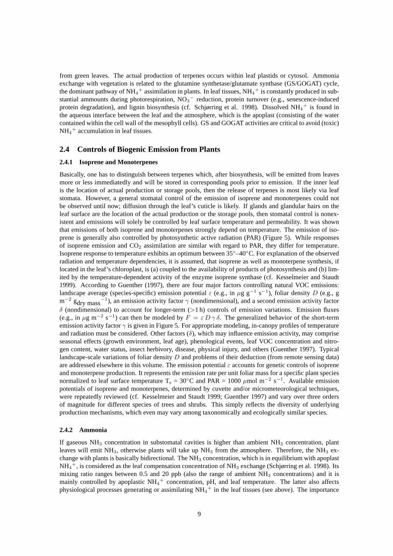
2.4 Controls of Biogenic Emission from Plants

2.4.1 Isoprene and Monoterpenes

Basically, one has to distinguish between terpenes which, after biosynthesis, will be emitted from leavesmore or less immediatedly and will be stored in corresponding pools prior to emission. If the inner leafis the location of actual production or storage pools, then the release of terpenes is most likely via leafstomata. However, a general stomatal control of the emission of isoprene and monoterpenes could notbe observed until now; diffusion through the leaf’s cuticle is likely. If glands and glandular hairs on theleaf surface are the location of the actual production or the storage pools, then stomatal control is nonex-istent and emissions will solely be controlled by leaf surface temperature and permeability. It was shownthat emissions of both isoprene and monoterpenes strongly depend on temperature. The emission of iso-prene is generally also controlled by photosynthetic active radiation (PAR) (Figure 5). While responsesof isoprene emission and CO2 assimilation are similar with regard to PAR, they differ for temperature.Isoprene response to temperature exhibits an optimum between 35◦–40◦C. For explanation of the observedradiation and temperature dependencies, it is assumed, that isoprene as well as monoterpene synthesis, iflocated in the leaf’s chloroplast, is (a) coupled to the availability of products of photosynthesis and (b) lim-ited by the temperature-dependent activity of the enzyme isoprene synthase (cf. Kesselmeier and Staudt1999). According to Guenther (1997), there are four major factors controlling natural VOC emissions:landscape average (species-specific) emission potentialε (e.g., inµg g−1 s−1), foliar densityD (e.g., gm−2 gdry mass

−1), an emission activity factorγ (nondimensional), and a second emission activity factorδ (nondimensional) to account for longer-term (>1 h) controls of emission variations. Emission fluxes(e.g., inµg m−2 s−1) can then be modeled byF = εD γ δ. The generalized behavior of the short-termemission activity factorγ is given in Figure 5. For appropriate modeling, in-canopy profiles of temperatureand radiation must be considered. Other factors (δ), which may influence emission activity, may compriseseasonal effects (growth environment, leaf age), phenological events, leaf VOC concentration and nitro-gen content, water status, insect herbivory, disease, physical injury, and others (Guenther 1997). Typicallandscape-scale variations of foliar densityD and problems of their deduction (from remote sensing data)are addressed elsewhere in this volume. The emission potentialε accounts for genetic controls of isopreneand monoterpene production. It represents the emission rate per unit foliar mass for a specific plant speciesnormalized to leaf surface temperature Ts = 30◦C and PAR = 1000µmol m−2 s−1. Available emissionpotentials of isoprene and monoterpenes, determined by cuvette and/or micrometeorological techniques,were repeatedly reviewed (cf. Kesselmeier and Staudt 1999; Guenther 1997) and vary over three ordersof magnitude for different species of trees and shrubs. This simply reflects the diversity of underlyingproduction mechanisms, which even may vary among taxonomically and ecologically similar species.

2.4.2 Ammonia

If gaseous NH3 concentration in substomatal cavities is higher than ambient NH3 concentration, plantleaves will emit NH3, otherwise plants will take up NH3 from the atmosphere. Therefore, the NH3 ex-change with plants is basically bidirectional. The NH3 concentration, which is in equilibrium with apoplastNH4

+, is considered as the leaf compensation concentration of NH3 exchange (Schjørring et al. 1998). Itsmixing ratio ranges between 0.5 and 20 ppb (also the range of ambient NH3 concentrations) and it ismainly controlled by apoplastic NH4+ concentration, pH, and leaf temperature. The latter also affectsphysiological processes generating or assimilating NH4

+ in the leaf tissues (see above). The importance

9

Figure 5: Generalized behavior of nondimensional actgivity factorsγ=γ(Ts) andγ=γ(PAR) for biogenicemissions of isoprenoids. Emission activity factors are used to scale plant species specific emission po-tentials to short-term variations of leaf surface temperature (Ts) and photosynthetic active radiation (PAR).Figures are taken from Kesselmeier and Staudt (1999).

10

Figure 6: The effect of increasing leaf temperature inBrassica napusplants exposed to 15 ppb NH3 atTair = 25◦C, PAR = 500µmol m−2 s−1, and r. h. = 20%. Plants were growing at a high nitrogensupply and (duplicate) measurements were performed during the vegetative growth state. The dashed line isdeduced from relevant thermodynamical equilibria at ambient NH3 concentration 15 ppbv (a temperature-independent leaf NH3 conductance of 0.12 mol m−2 s−1 was assumed). Figure taken from Schjørring etal. (1998).

of leaf temperature is demonstrated in Figure 6: under controlled environmental and nutritional conditions,increasing leaf temperature switches the NH3 exchange status from deposition to emission. Diffusion intoand out of the plant leaves was found to be entirely controlled by stomatal openings. However, it wasobserved that the leaf NH3 conductance varies with the nitrogen status of the plant (Schjørring et al. 1998).Furthermore, the plant’s nitrogen uptake (from the root medium in the form of NO3

− or NH4+) affects the

strength of NH3 emission: NH4+-absorbing plants emit considerably more NH3 than those which absorbNO3

−. Assimilation, (internal) transport and turnover of nitrogen change dramatically over the variousstages of plant development: a bimodal pattern of the NH3 compensation point of cereals is generallyfound (with maxima around tillering and grain filling, separately).

2.4.3 Nitric Oxide

Very recently, biogenic NO emission from a variety of plant species was observed by Wildt et al. (1996)during laboratory fumigation experiments at low ambient NO concentrations. For the plants studied so far(sunflower, sugar cane, soybean, corn, rape, spruce, spinach, and tobacco) they suggest an NO compen-sation point around 1 ppb. The nature of plant physiological processes that emit NO is almost unkown.However, a first-order relationship between rates of daytime NO emission and uptake rates of CO2 wasobserved (3× 10−6 mol of NO emitted per mole CO2 taken up). Based on this relation, the global strengthof NO emission by plants may be in the order of 2.4 Tg N y−1.

2.5 Landscape Pattern Control over Biogenic Emissions: Some Examples

Soil water, due to its outstanding role in plant physiology, substrate (trace gas precursor) production, anddiffusivity of trace gases could certainly be considered as the most important controlling factor amongthose discussed above. However, temporal and spatial distribution of (surface) soil water results from mi-croclimatic and hydrological conditions in the landscape, which are usually modified by landforms (whichcomprise the landscape). In turn, the type and intensity of key factors for plants and soils (and hence,patterns of soils and plants at a site) are largely controlled by these land form-influenced environmentalconditions. Therefore, biogenic emissions of trace gases, particulary those from soils, should be prone tocharacteristic variations of landforms best studied along toposequences (e.g., Figure 7).

11



ecosystemtype

transportprocess

oxidation process

� diffusion almost complete reoxidation in the water co-lumn at the oxycline; ± permanent CH4

emission

� diffusion almost complete reoxidation in the oxic sur-face sediment; ± permanent CH 4 emission

� ebullit ion almost no reoxidation; ± permanent CH4

emission

� vasculartransport

reoxidation in the rhizosphere (depends onvascular transport of O 2 and respiration inrhizosphere) ; ± permanent CH4 emission

� diffusion temporary CH4 production (due to submer-gence or stagnant water); change betweenCH 4 emission and CH 4 deposition

� diffusion ± permanent CH 4 deposition

Figure 7 : Soil transport and oxidation processes involved in CH4 cycling between terrestrial

ecosystems and the atmosphere (figure taken from: Conrad, R. 1989. Control of

methane production in terrestrial ecosystems. In: Exchange of trace gases between

terrestrial ecosystems and the atmosphere, eds. M.O. Andreae and D.S. Schimel, pp.

39-58. Chichester, New York: John Wiley & Sons Ltd.)

Figure 7: Soil transport and oxidation processes involved in CH4 cycling between terrestrial ecosystemsand the atmosphere (Conrad 1989).

The inserted table in Figure 7 summarizes CH4 oxidation processes and CH4transport processes al-ready described above under the sectionsMethane ProductionandMethane Oxidation. These are mainlycontrolled by (seasonal) inundation, changes in water table height, and soil moisture content; as thesehydrological quantities vary with landscape/landform pattern, CH4 exchange will also vary. While the(surface) soil moisture content (and soil temperature) will determine the intensity of CH4 deposition withinecosystem type 6, special emphasis sould be put on type 5 (Figure 7). In this system, the water table heightmay switch parts of or the entire (periodically drying) wetland ecosystem from a significant CH4 sourceto a significant CH4 sink (Bartlett and Harriss 1993). For northern boreal peatlands, spatial scales of thevariability of CH4 exchange were recently reported by Waddington and Roulet (1996): seasonally averagedCH4 emissions ranged over up to three orders of magnitude between hummocks and hollows (3 m scale),ridges, lawns and pools (100 m scale), and on the landform scale (500 m).

In case of N2O emissions from cultivated soils, high spatial variability of soil microbial activity isusually considered to prevent the development of predictive relationships between factors which impact agiven microbial process. However, Corre et al. (1996) showed that such relationships can be derived if anappropriate spatial sampling scheme is used and those statistical measures for data evaluation, which areresistant to the effects of few extreme values, are applied. Some of their results are summarized in Figure 8.With the exception of the pasture site, a significant pattern on the landscape-scale (50–250 m) was observed,showing higher N2O emissions on the footslope than on the shoulder complexes. As suggested by theinserted schematic in Figure 8, the lower N2O emission activity associated with the shoulder comparedwith the footslope complex reflects the influence of topographically induced water redistribution and betterinternal drainage conditions of the soils on the upper than on the lower landscape conditions. Corre et al.(1996) conclude that, during their study in the Canadian Black soil zone, only a discrete number of factorscontrolled the N2O flux variability, namely, soil-parent sediment, vegetation–land-use pattern, climate, andtopography. They present a concept of links between large-scale controllers and proximal factors of N2Oemissions which is shown in Figure 9.

As already mentioned in sectionSoil Water Content and Gaseous Diffusivity(see also Figure 3), thepartition of gaseous nitrogen emissions between NO, N2O, and N2 depends strongly on the actual soilmoisture content. If we accept general validity of the observations by Corre et al. (1996), we would expecthigher NO emissions from shoulder than from footslope complexes of areas of similar geomorphologicalcharacteristics. In case of NO emissions, it has also to be emphasized that the controlling processes are most

12

Figure 8: Landscape patterns of N2O emissions (May, 1993, to May, 1995) form the black soil zone (UdicBoroll soils) near St. Louis, Saskatchewan, Canada (data are taken from Corre et al. 1996). Basic landform classification (2 = shoulder complex, = footslope complex) are from Pennock et al. (1994). Theinsert shows a summary diagram of probable water movement and concentration associated with differentlandform elements in a hillslope system (from Pennock et al. 1987).

Figure 9: Conceptual links between large-scale controllers and proximal factors of N2O emissions (afterCorre et al. 1996).

13

likely confined to the uppermost soil layers (0–3 cm; cf. Remde et al. 1993, Meixner 1994). Therefore,diurnal effects of surface soil temperature and wetness may result in more short-term variations of NOemissions as compared to N2O emissions. Also unlike N2O, NO is highly reactive in the atmosphere andconverts (by reaction with ozone) rapidly to NO2, which in turn is photolyzed back to NO on a similar timescale under daylight conditions (cf. Remde et al. 1993). However, within vegetation canopies, biogenicNO from soil will partly be converted to NO2, since shadowing by vegetation elements will more or lesssuppress NO2 photolysis. Uptake of NO2 by vegetation elements is small but still an order of magnitudelarger than that for NO (cf. Meixner 1994). As a result, not all of the NO emitted from soils may escapeto the atmospheric boundary layer (ABL). First estimates of the so-called “canopy reduction” of soil NOemission range within some ten percent; quantification on local and/or regional scales is lacking.

3 Transport and Deposition Processes in Complex Landscapes

Transport processes in complex landscapes with variable topography and small- to large-scale differencesin land use are strongly affected by local wind systems, which develop owing to differential surface heatingand differences in surface moisture (see Pielke et al., this volume). In general, the transport of a trace gasin the atmosphere ends with the deposition to the Earth’s surface or with chemical depletion (which is notconsidered here). In this chapter we do not address all transport and deposition processes in detail butrestrict ourselves to the most specific onces for complex landscapes.

3.1 Sea- and Land-breeze Systems, and the Effect of Large-Scale Differences inLand Use

We start our discussion of the transport processes at the largest scale considered in the present context,which is less than 100 km in the horizontal direction. On this scale, the most spectacular transport processesare related to photochemical smog problems, e.g., those of Los Angeles and Athens. The daytime sea-breeze wind system transports pollutants from the seashore into the urban area, where they are trappedby local topography (mountain barrier), while at night, when the land surface becomes colder than the seasurface, the trapped pollutants are blown back to the sea without the possibility of rapid turbulent dispersioninto the free troposphere, as would be the general case in flat and level terrain.

Although topography is the main factor in this example, Zhong and Doran (1995) showed that regionalvariation in the land-use pattern might even have a stronger effect on atmospheric transport than topog-raphy alone, even in complex terrain. In a modeling excercise on the regional distribution of (potential)temperature and wind fields over a rural area in northwestern U.S.A., they demonstrated that model runsconsidering actual topography and different land use (steppe vs. irrigated farmland or open water surface)represented observed fields more closely when topography was neglected than when land use was neglected(Figure 10).

However, the question of how large areas of different land-use pattern must be to have a significantinfluence on the regional scale still remains open. For instance, aircraft transect flights addressing thetransition from dry to irrigated farmland (Pielke and Avissar 1990; Mahrt et al. 1994) showed that thetransition of (potential) temperature was gradual (rather than stepwise) and extended over a horizontaldistance of more than 10 km (at flight levels of 140 m and more above ground; Pielke and Avissar 1990)to a few km (at flight levels of 30 m; Mahrt et al. 1994). Thus, for most areas of the world where land-usepatterns change at the smaller scale of a few tens to hundreds of meters, the importance of such land-usedifferences seems to lie primarily in the alteration of turbulent exchange with the surface within the surfacelayer.

3.2 Valley and Slope Wind Systems, and the Recirculation of Trace Substances

Valley and slope wind systems were initially described for deep and long moutain valleys. There, a persis-tent diel wind direction pattern with frequently high wind speeds (typically on the order of 10–20 m s−1 invalleys like the Kaligandaki valley of Nepal) can be observed not only by the educated meteorologists. Theimportance of valley and slope wind systems for the transport and recirculation of atmospheric consitutents

14

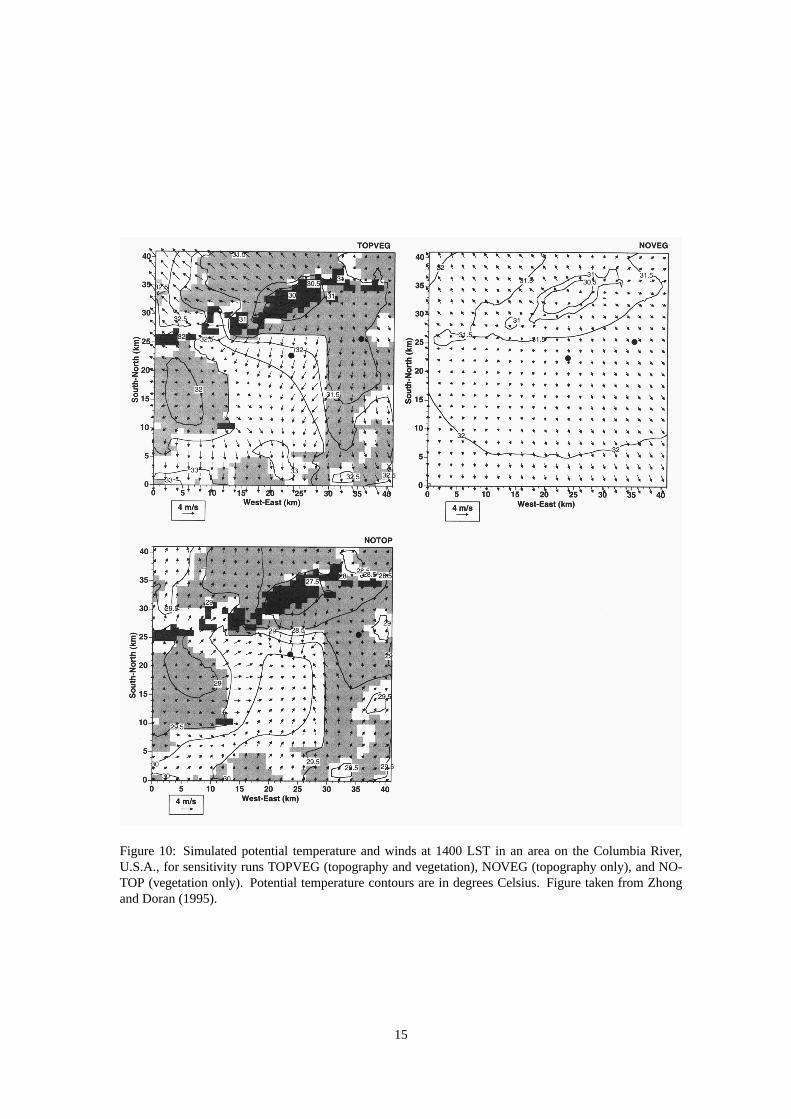
Figure 10: Simulated potential temperature and winds at 1400 LST in an area on the Columbia River,U.S.A., for sensitivity runs TOPVEG (topography and vegetation), NOVEG (topography only), and NO-TOP (vegetation only). Potential temperature contours are in degrees Celsius. Figure taken from Zhongand Doran (1995).

15

was recently shown by Allwine and Whiteman (1994) for the Grand Canyon region. Although with lesssevere restrictions on dispersion and transport due to the local topography, similar influences of landscapepatterns and topography can be expected in moderately complex terrain. This is due to the interaction be-tween the lateral topographic restrictions of the air volume in which trace gases are dispersed and the heightof the ABL. Usually, a (temperature) inversion is topping the ABL within which most surface-emitted tracegases are trapped owing to the very weak turbulent exchange across the inversion layer. For moderatelycomplex topography with differences in elevation less than 400 m, the top of the noon and early afternoonABL is typically higher than the peaks of local topography. Therefore, the restrictions on lateral disper-sion due to topography are limited to late afternoon, nighttime and early morning periods, when the ABLheight may be less than the peak heights of local topography. In deep mountain valleys even the maxi-mum daytime ABL height may stay below the moutain crests, which significantly reduces the atmosphericvolume into which surface emitted trace gases can be dispersed. The simple concept of the topographicamplification factor (TAF) (Whiteman 1990) illustrates this for air temperature, but is also applicable tothe transport of trace substances. In complex terrain, there is a smaller volume of air inside a box with thebottom defined by the terrain elevation, compared to a box of the same size over flat terrain. Additionally,the real surface of the topography inside the complex terrain box is larger than the corresponding surfaceof the flat terrain. Given a constant incoming solar radiation flux density, this causes the larger surface toheat a smaller volume, and hence the higher air temperatures are higher over complex terrain than overflat topography. By analogy, the concentration of a trace gas emitted from complex terrain should be, inprinciple, higher than over flat terrain, as the larger surface area would emit the trace gas into a smallervolume of air. However, we showed above underSoil Temperaturethat surface (soil) temperature may bea major influencing factor for the biogenic emission of many trace gases and the response to it is generallyexponential. On the other hand, there is the dependence of surface temperatures on slope angle and orien-tation (e.g., Swift 1976). Therefore, it cannot be said a priori that a complex topography will directly resultin higher overall emissions only owing to its larger surface: some of the area in complex terrain would cer-tainly have significantly lower surface temperature owing to its exposition away from the sun, which mayreduce overall emissions as compared to a flat plain with the same projected surface area. Soil moistureis probably themostimportant factor for emissions, especially for methane (water table controls whetherCH4 is emitted or taken up by soils). Surface soil moisture on slopes is not only controlled by radiativeinput and thus exposure of the slope, but also by subsurface flows of water. If subsurface flow is absent,then the slopes exposed towards the sun are drier and warmer compared with those exposed away from thesun, potentially leading to a moisture limitation of soil emission processes or to a temperature limitation inthe second case.

3.3 Air-mass Blocking and Cavities

An important factor for atmospheric transport in complex terrain is air-mass blocking in front of cavitiesor behind obstacles, owing to deceleration of atmospheric flow. This can be seen on all scales from wholemountain systems down to exposed single hills, forest edges, and buildings, when the atmosphere is stablystratified. Depending on the strength of atmospheric stability and the size of the obstacle, atmosphericflow will be either around (small Froude numbers,Fr, very stable stratification with weak winds) or overobstacles (highFr, slightly stable stratification with moderate to strong winds), or a combination of both.On the upwind side (upwind cold-air blocking, lowFr) or on the downwind side (lee-side rotor cavity,intermediateFr), trace gases may accumulate and lead to both higher concentrations and higher surfacedeposition than the regional average. Additionally, wind direction and wind speed can differ considerablyin blocked air mass owing to the decoupling from the atmosphere aloft. This is often the case in valleyswhen synoptic winds are perpendicular to the valley (Whiteman and Doran 1993). In such cases, theatmosphere inside the valley may be decoupled from the atmosphere aloft, which can have significantimpact on the direction of atmospheric transport and vertical dispersion at the interface between the blockedair near the surface and the rest of the ABL aloft. The general pattern based on the Froude number is thefollowing: during weak wind conditions with (very) stable stratification, air pollutants accumulate upwindof an obstacle; while at higher wind speed and decreased stability, air pollutants tend to trap behind theobstacle in a cavity.

16

3.4 Orographic Effects: The Seeder–Feeder Mechanism

The picture gets even more complicated in the presence of clouds. Fowler et al. (1995) found that theconcentration of major pollutant ions (Cl−, SO4

2−, NO3−, NH4

+) in the cloud water is related to therelative proximity of a site to marine or anthropogenic sources of aerosol. However, they also found thatconcentrations in orographic clouds (e.g., “cap clouds” around summits, generated by the forced ascent ofmoist air on a mountain barrier) exceed those in frontal (upwind) clouds by a factor of five to ten, leadingto 20%–50% higher wet deposition at summit sites compared to low ground locations. This importantinfluence of topography on transport and deposition of dissolved pollutants is called the seeder–feedermechanism: rain droplets from frontal clouds (seeder) in higher levels are incorporated in orographical capclouds (feeder), where pollutants accumulate before they are wet deposited to the surface. In addition tothe dissolved pollutants received from the seeder clouds, orographical clouds may scavenge trace gases andaerosol particles out of the upwind air mass, thus further influencing the transport and wet deposition ofsuch constituents in complex landscapes. Such orographic effects may shift the ratio between dry and wetdeposition towards increased wet deposition.

3.5 Forest Edges, Changes in Displacement Height, and the Smooth-to-rough Tran-sition

Along forest edges and wherever surface roughness suddenly increases or a considerable step of the heightof roughness elements occurs (i.e., where the so-called aerodynamic displacement height increases), thereis an aerodynamic effect that may lead to enhanced dry deposition of trace gases and particles, as well as ofenhanced interception of fog droplets at some (short) distance from the edge line. This is due to a rotatingturbulence element which is created at the edge. It will lead to persistent downdrafts at a downwinddistance of the turbulence element’s average size from the edge line. This is also the range of highestdynamic pressure, where most windfelled trees can be found, and agricultural crops are most likely bentdown at some distance from the field edge after the passage of a thunderstorm. Draaijers et al. (1994)performed a field experiment at eight forest edges and showed that current deposition models underestimatedeposition of acidifying compounds to Dutch forests by 10% just owing to edge effects. Although theirfocus was on forest edges, this phenomenon is not restricted to forest edges alone but also to any similarcondition in a landscape. As the total length per unit area of edge lines (between surfaces of differentroughness-displacement height) increases with the complexity of landscape pattern and vegetation mosaic,we expect biased estimates of both transport and exchange of trace substances in complex terrain, if thebasic assumptions in the corresponding modeling approach is based on homogeneous and flat surface.We think that this may generally lead to a systematic underestimation of local deposition and thus to anoverestimation of horizontal transport distances in complex landscapes.

3.6 Rough-to-smooth Transition and Other Roughness Length Effects

Together with atmospheric stability (i.e., the thermal structure of the ABL), the aerodynamic roughness ofa surface determines the turbulent structure (the vertical turbulent exchange) and the vertical wind profile(the vertical shape of horizontal transport) in the ABL. There is an important difference of total surfaceroughness between homogeneous terrain and patchy landscapes, where very frequent transitions from asmooth to a rough surfaces and vice versa occur. Over horizontally homogeneous terrain, the aerodynamicroughness of the surface can be described by only the geometry and density of the vegetation elementsgrowing on the surface or by the size of small-scale structures of nonvegetated surfaces (e.g., wave heightover water surfaces). However, in complex terrain, the total aerodynamic roughness of the landscape isa composite of local surface roughness plus the roughness of the (bare) topography, which is generallya few orders of magnitude larger than the local surface roughness. Thus, aerodynamic roughness is notscale-invariant. Models will use different values, depending on spatial resolution and thus on the scale ofprocesses which are explicitely modeled. Due to the fact that turbulence is generated almost immediatelyat a smooth to rough transition, the decay of this turbulence at the rough to smooth transition is governedby the internal properties of the flow, the dissipation rate for kinetic energy, which has a much longer timeconstant than the generation of turbulence. Thus, the atmosphere above a landscape with frequent changes

17

in surface roughness has a higher grade of turbulence than a homogeneous landscape, and the effect ofmechanic turbulence created over complex topography adds to this landscape-influenced turbulence. Theconsequences for transport of constituents in the atmosphere are identical to those already stated for theforest edge effect: over complex landscapes we expect increased turbulence, which leads to increaseddeposition and thus to decreased horizontal transport distances compared to horizontally homogeneouslandscapes. Because the concentration of trace gases in the atmosphere is extremely low, there is no back-pressure effect induced by increased deposition and decreased transport distances over rough surfaces thatwould lead to an increase or reduction of trace gas emissions.

3.7 The Laminar-turbulent Transfer Resistance

So far, our description of transport processes considered turbulent and mesoscale scales, which are roughlythree orders of magnitude more efficient for dispersion of consituents in the atmosphere than moleculardiffusion. However, very close to the surface, around any vegetation element, object, obstacle, etc. thereis a quasi-laminar layer of air, which is only a few tens of micro- or millimeters depth. Transfer acrossthis quasi-laminar layer may be an essential control both for the exchange (emission and deposition) oftrace substances. Given the rough guess of the efficiencies of turbulent versus molecular diffusion, one canestimate that it should take an atmospheric constituent as long to cross a 1 mm quasi-laminar layer as itwould take it to travel 1 m in the turbulent ABL. The depth of this quasi-laminar layer depends mainly onwind speed and other micrometeorological parameters, but also on the shape and size of the object.

3.8 Internal Boundary Layers, Fetch and Footprint, and the Urban Heat Island

Changes in landscape pattern are almost always associated with changes in surface roughness, albedo, sur-face moisture, plant activity, and thus surface energy balance. Such changes induce new internal boundarylayers due to changes in mechanic turbulence production (especially at the smooth-to-rough transition) andthermal convection (due to changes in sensible heat flux). The urban heat island is an example of such aninternal boundary layer resulting from increased sensible heat flux from urban areas (where surface wateravailability is low and thus evapotranspiration is small). Raupach (1993) has shown that there are threekinds of heterogeneity to be considered:

1. microscale heterogeneity between adjacient surface patches for which advection occurs in the surfacelayer;

2. mesoscale heterogeneity for which the ABL is well-mixed, but advection occurs on the scale of theABL; and

3. macroscale heterogeneity for which advection is negligible and surface patches are energeticallyindependent.

Currently there are two experimental concepts used by micrometeorologists to deal with inhomo-geneities in landscape:

1. Flux measurements are made in the surface layer as close to the canopy as possible to get measure-ments that are representative of a distinctive surface or vegetation type due to its small footprint (areathat influences the flux measurement) (Schmid and Oke 1990).

2. Flux measurements are made on a tall tower 10–100 m or with an aircraft to get flux measurementsthat represent an average of a large area and thus integrate over all the patches represented in thefootprint of the measurement.

The remaining key question, however, is: what is the footprint of a measurement and how representativeare any of the flux measurements taken with either measuring concept? The concepts of instrument fetch(the upwind distance, which must be homogeneous to allow equilibration of the atmospheric flow with thatsurface) and the footprint (the contributing surface area for a measurement) are both based on homogeneousand idealized conditions. For example, a change in roughness is most often also in direct combination with

18

a change in displacement height. However, footprint models neglect differences in displacement height,not to mention complex topography. This may lead to severe errors in estimation of footprint areas incomplex landscapes. However, there is some general agreement that, although imperfect, such footprintmodels are a valid tool to assess the problem of spatial representativity of flux measurements obtained overnonhomogeneous and nonflat terrain.

The independent variables in the Flux Source Area Model by Schmid and Oke (1990) are the ratio be-tween measuring height and surface roughness (z/z0), the atmospheric stability (z/L), and the turbulenceparameter for lateral turbulence (σv/u∗) which determines the width of the footprint. While largez/z0 leadto large footprints, any increase ofz0 due to landscape pattern and complex terrain automatically results inthe reduction of the the footprint size, while lateral dispersion typically increases over such landscapes, andthus, the flux footprint area gets wider. In general, it seems possible to extend atmospheric flux measure-ments, which are best described for horizontally homogeneous and flat landscape, to complex terrain andpatchy landscape, if they are accompanied with careful investigation of the flux footprint in order to knowwhat flux measurements obtained in nonideal terrain actually represent. In most cases, a good startingpoint is to investigate the dependence of a flux measurement on wind direction (e.g., Jarvis et al. 1997).Such an analysis reveals many features that can be directly explained by local heterogeneities within thefootprint area. Although the size of the footprint area may not be accurately estimated by a footprint modelthat was designed for homogeneous topography, the order of magnitude is expected to be correct even incomplex landscape and is an indication of where to search for surface heterogeneities that may explain themeasured dependence of flux on wind direction. A further refinement would include a classification of themeasuring conditions according to atmospheric stability, which strongly influences the horizontal extent ofthe footprint area.

3.9 Effects of Atmospheric Stability: Katabatic Drainage Flow and Cold Air Lakes

We cannot make a priori statements about the effect of landscape pattern and topography on emission andtransport which are generally be valid for any and all types of complex landscapes. Atmospheric stabilityinfluences all of the above listed transport processes, and atmospheric stability depends on (a) net radiativeinput (which varies with time of day and season); (b) how this energy is partitioned into sensible, latent,and ground heat flux at the surface (the fraction converted to sensible heat flux directly affects atmosphericstability); and (c) mechanical turbulence driven by the wind shear in the surface layer. All these propertiesare influenced by complex terrain and a vegetation mosaic in a nonlinear way such that their influence onatmospheric stability and transport must be studied seperately for each unique study area of the world. Evenwell-known and widely accepted models about processes like katabatic drainage flow (bringing cold air andits consituents from higher elevations into basins and valleys during nighttime) do not necessarily lead toidentical results in similar landscapes. In one case, drainage flow may lead to deep cold air lakes withsurface fog, while in another case there is no fog and cold air is not pooling within the study domain. Thismay be due to differences in orientation of the complex landscape: in south-going valleys of the northernhemisphere, the daytime up-valley wind is generally stronger than the nocturnal down-valley wind, while avalley with identical shape and topographic relief that is opening to the north may show a weaker daytimeup-valley wind and a stronger nocturnal down-valley wind, a difference that only results from exposuredifferences, not differences in landscape patterning, topographic relief, or the vegetation mosaic.

4 Open Questions, Points of Controversy, Research Needs

Our description of effects of landscape and topography on emission and transport addresses a very widerange of scales for the processes involved, with the smallest scale for the microbial processes describedunder the sectionEMISSIONS OF TRACE GASES FROM SOILS AND VEGETATION , and a larger scalefor the atmospheric processes inTRANSPORT AND DEPOSITION PROCESSES IN COMPLEX L AND-SCAPES, where we emphasize the small-scale processes with a more detailed description. This simplyreflects the fact that, unlike for transport (as well as for water and CO2 exchange), research on the biogenicemission of most trace gases is comparably young and still needs basic mechanistic studies for under-standing. In contrast, research on turbulent transports has reached a more advanced state of scientific

19

understanding, thanks to all the well-funded research that was carried out in the past few decades in thefields of aircraft engineering and atmospheric dispersion of radioactive substances that would occur follow-ing a nuclear strike. To link small-scale heterogeneity with the large-scale atmospheric processes is alsothe key issue. We believe, that despite some obvious success of previous large-field experiments, there arestill plenty of open questions to be addressed here.

Under the consensus that the microscopic level of microorganisms’ metabolism exerts anyinitial con-trol over biogenic emissions (Conrad 1996), the open question that still remain are:

1. What are the consequences of the vast microbial diversity in plants and soils for higher levels oforganisation and control?

2. Can we—as for energy, CO2 and H2O (see Valentini et al., this volume)—define any spatial unit(s)on which biogenic emission of a given trace gas shows a coordinated and specific response to envi-ronmental factors?

3. What is the appropriate level of control (microbial community, soil crumbs, vegetation elements,(whole) species, patch, biome) where the development of functional relationships (for extrapolationto larger spatial and temporal scales) can start?

There is some discussion (not even controversy) to which extent the diversity of microorganisms mattersin terms of trace gas emissions. While Conrad (1996) favors microbial species diversity as an importantfactor in ecosystem function, Schimel (1995) asks whether the microbial diversity and community structurein soil have any consequences at the ecosystem level. However, there is growing interest with respect tofunctional groups of microbes (rather than on species of microorganisms) for identification of factors whichcontrol rates of production and consumption (Davidson and Schimel 1995). Simple concepts on how todeal with the effects of nonhomogeneous and nonflat landscapes do not exist, neither for biogenic emissionsnor for atmospheric transport. Major points of controversy in this respect exist on where and how to doexperimental measurements in order to get representative data sets for an extended area (e.g., a region).The most widespread concept to date is to select locations that are only disturbed by as few heterogeneitiesand as little terrain relief as is unavoidable in a given region. A second concept, which is finding moreacceptance within the scientific community, is to view landscape heterogeneity and complex terrain issuesas a challenge, based on the understanding that this is the real world. Another concept, although it utilizesa better theoretical base so far, does not address the real situation of large areas of the Earth’s land surface.The drawback, however, is the need for additional data that are not required in studies carried out in flatand homogeneous landscapes. However, we believe that the scientific community has already begun todevelop the right tools for understanding complex landscapes, such that the expenses needed for measuringadditional data can be scientifically justified. Two key questions addressing these scientific tools weresupplied by one of the reviewing workshop participants:

1. How can the relationships between large-scale landscape pattern, small-scale spatial heterogeneity,and emission of trace gases be quantitatively related?

2. How can spatial variability be handled by appropriate experimental designs?

We think that the most promising approach to answer the first question is spatial explicit modelingwith a dynamic atmospheric model that incorporates a mosaic of small-scale land use (and thus trace gasemissions sources) for each model grid cell with a resolution that suits the subgrid scale heterogeneity ofcomplex landscapes. We suggest that the required grid resolution, depending on the application, should be1 km2 (or finer) and the mosaic within each grid cell must be able to resolve surface heterogeneities on thescale of 10×10 m2 plots. An approach to develop the methodology addressing the second question waspresented by Eugster et al. (1997). The general idea is similar to what has been practiced in climatology fordecades: long-term (anchor) stations should provide flux measurements against which short-term measure-ments from various localities in a complex landscape can be cross-referenced to address spatial variability.Furthermore, as in the field study of Corre et al. (1996), spatial sampling schemes for biogenic emissions,which are tailored to the particular local situation, should be developed; and those statistical measures fordata evaluation, which are resistant to the effects of few extreme values, should be applied. Difficult and

20

unresolved problems, however, lie in the statistical integration of such spatiotemporal data sets. Wikle andCressie (1999) presented a statistical approach for measurements obtained from research vessels, and weexpect that similar approaches will be extended to land surfaces and, especially, complex landscapes in thenear future.

Research needs may be summarized as:

• continuing field experiment on biogenic emission of trace gases from carefully selected key ecosys-tems of the globeand laboratory experiments on the corresponding soils and plants;

• finding more generally applicable theories on where to measure and how to measure nonideal land-scapes in order to be able to receive accurate regional estimates;

• separating local problems from general problems within different types of complex landscapes;

• defining the time lags and scales of processes which are affected by landscape pattern and topography(e.g., inundations, pollutant-rich cold-air lakes); and

• improving knowledge on how land-use changes, anthropogenic activities (in a widest sense), climatevariability, and climate change interact with each other on the landscape scale (human dimensionsaspect not addressed herein).

Clearly, for biogenic emissions, solutions to methodological problems will promote field studies fo-cusing on increasingly complex landscapes, and the complementary laboratory experiments, under well-defined conditions, will increase knowledge of underlying mechanisms and quantify controlling factors,provided the applicability of laboratory results to field conditions is guaranteed.

Acknowledgments

We acknowledge generous support received from the Universities of Bern and Bayreuth (WE), and the MaxPlanck Institute for Chemistry, Mainz (FXM) to work on this paper. Many thanks to Ms. Carol Strametzfor improving the language and style of this paper considerably.

ReferencesAllwine, K. J., and C. D. Whiteman. 1994. Single-station integral measures of atmospheric stagnation, recirculation and ventilation.

Atmospheric Environment28: 713–721.

Andreae, M. O., and P. J. Crutzen. 1997. Atmospheric aerosols: Biogeochemical sources and role in atmospheric chemistry.Science,276: 1052–1058.

Andreae, M. O., and W. A. Jaeschke. 1992. Exchange of sulfure between biosphere and atmosphere over temperate and tropicalregions. In: Sulfure Cycling on the Continents Systems and Wetlands, ed. R. W. Howarth, J. W. B. Stewart, and M. V. Ivanov,pp. 27–61. Chichester: Wiley.

Andreae, M. O., and D. S. Schimel. 1989. Exchange of trace gases between terrestrial ecosystems and the atmosphere. DahlemKonferenzen. John Wiley & Sons Ltd., Chichester, U.K.

Bartlett, K. B., and R. C. Harriss. 1993. Review and assessment of methane emissions from wetlands.Chemosphere26 (1–4):261–320.

Conrad, R. 1989. Control of methane production in terrestrial ecosystems. In: Exchange of Trace Gases between Terrestrial Ecosys-tems and the Atmosphere, ed. M. O. Andreae and D. S. Schimel, pp. 39–58. Dahlem Workshop Report LS 47. Chichester:Wiley.

Conrad, R. 1994. Compensation concentration as critical variable for regulating the flux of trace gases between soil and atmosphere.Biogeochemistry. 27: 155–170.

Conrad, R. 1996. Soil microorganisms as controllers of atmospheric trace gases (H2, CO, CH4, OCS, N2O, and NO),MicrobiologicalReviews, 60 (4), 609–640.

Corre, M. D., C. van Kessel, and D. J. Pennock. 1996. Landscape and seasonal patterns of nitrous oxide emissions in a semiaridregion.Soil Sci. Soc. Am. J. 60: 1806–1815).

Davidson, E. A., and Schimel, J. P. 1995. Microbial processes of production and consumption of nitric oxide, nitrous oxide andmethane. In: Biogenic trace gases: measuring emissions from soil and water, eds. P.A. Matson and R.C. Harriss, pp. 327–357. Oxford: Blackwell Scientific Publications Ltd.

21

Draaijers, G. P. J., R. van Ek, and W. Bleuten. 1994. Atmospheric deposition in complex forest landscapes.Boundary-LayerMeteorol. 69: 343–366.

Eugster, W., J. P. McFadden, and F. S. Chapin III. 1997. A comparative approach to regional variation in surface fluxes using mobileeddy correlation towers.Boundary-Layer Meteorol.85: 293–307.

Fowler, D., I. D. Leith, J. Binnie, A. Crossley, D. W. F. Inglis, T. W. Choularton, M. Gay, J. W. S. Longhurst and D. E. Conland.1995a. Orographic enhancement of wet deposition in the United Kingdom: continuous monitoring.Water, Air and SoilPollution85: 2107–2112.

Galbally I. E., and C. Johansson. 1989. A model relating laboratory measurements of rates of nitric oxide production and fieldmeasurements of nitric oxides from soils.J. Geophys. Res. 94: 6473–6480.

Guenther, A. 1997. Seasonal and spatial variations in natural volatile organic compound emissions.Ecological Applications7 (1):34–45.

Jarvis, P. G., J. M. Massheder, S. E. Hale, J. B. Moncrieff, M. Rayment, and S. L. Scott. 1997. Seasonal variation of carbon dioxide,water vapor, and energy exchanges of a boreal black spruce forest.J. Geophys. Res.102: 28,953–28,966.

Kesselmeier, J., P. Schroder, and J. W. Erisman. 1997. Exchange of sulfure gases between biosphere and the atmosphere. In:Transport and Chemical Transformation of Pollutants in the Troposphere, ed. P. Borrel, P. M. Borrel, T. Cvitas, K. Kelly,and W. Seiler, vol. 4, Biosphere–Atmsophere Exchange of Pollutants and Trace Substances, ed. J. Slanina, pp. 176–198.Heidelberg: Springer.

Kesselmeier, J., and M. Staudt. 1999. Emissions of biogenic volatile hydrocarbons—A review.J. Atmos. Chem., in press.

Ludwig, J. 1994. Untersuchungen zum Austausch von Stickoxiden zwischen Biosphare und Atmosphare. Ph.D. diss., Univ. ofBayreuth, Germany.

Mahrt, L., J. I. MacPherson, and R. Desjardins. 1994. Observations of fluxes over heterogeneous surfaces.Boundary-Layer Meteorol.67: 345–367.

Matson, P. A., and R. C. Harriss. 1995. Biogenic trace gases: measuring emissions from soil and water. Oxford: Blackwell ScientificPublications Ltd.

Meixner, F. X. 1994. Surface exchange of odd nitrogen oxides,Nova Acta Leopoldina NF70 (288): 299–348.

Meixner, F. X., Th. Fickinger, L. Marufu, D. Serca, F. J. Nathaus, E. Makina, L. Mukurumbira, and M. O. Andreae. 1997. Preliminaryresults on nitric oxide emission from a southern African savanna ecosystem,Nutrient Cycling in Agroecosystems48 (1-2):123–138.

Pennock, D. J., D. W. Anderson, and E. de Jong. 1994. Landscape-scale changes in indicators of soil quality due to cultivation inSaskatchewan, Canada.Geoderma, 64: 1–19.

Pennock, D. J., B. J. Zebarth, and E. de Jong. 1987. Landform classification and soil distribution in hummocky terrain, inSaskatchewan, Canada.Geoderma, 40: 297–315.

Pielke, R. A., and R. Avissar. 1990. Influence of landscape structure on local and regional climate.Landscape Ecology4: 133–155.

Potter, C. S., Matson P. A., Vitousek P. M., Davidson E. A. 1996. Process modeling of controls on nitrogen trace gas emission fromsoils worldwide.J. Geophys. Res. 101: 1361–1377.

Ramanathan, V., L. Callis, R. Cess, J. Hansen, I. Isaksen, W. Kuhn, A. Lacis, F. Luther, J. Mahlman, R. Reck, and M. Schlesinger.1987. Climate-chemical interactions and effects of changing atmospheric trace gases.Rev. Geophys. 25: 1441–1482.

Raupach, M. R. 1993. The averaging of surface flux densities in heterogeneous landscapes. Exchange Processes at the Land Surfacefor a Range of Space and Time Scales (Proceedings of the Yokohama Symposium, July 1993). IAHS Publ. no. 212, 343–355.

Remde A., J. Ludwig, F. X. Meixner, and R. Conrad. 1993. A study to explain the emission of nitric oxide from a marsh soil.J.Atmos. Chem. 17: 249–275.

Schade, G. 1997. CO Emissions from Degrading Plant Litter. Ph.D. diss., J. Gutenberg Univ., Mainz, Germany.

Schimel, J. P. 1995. Ecosystem consequences of microbial diversity and community structures.Ecol. Stud. (Berlin)113: 239–254.

Schjørring, J. K., S. Husted, and M. Mattson. 1998. Physiological parameters controlling plant-atmosphere ammonia exchange,Atmos. Environ., in press.

Schmid, H. P., and T. R. Oke. 1990. A model to estimate the source area contributing to turbulent exchange in the surface layer overpatchy terrain.Q. J. R. Meteorol. Soc.116: 965–988.

Seiler, W., and R. Conrad. 1987. Contribution of tropical ecosystems to the global budget of trace gases, especially CH4, H2, CO,and N2O. In: The Geophysiology of Amazonia, ed. R. E. Dickinson, pp. 133–162. Chichester: Wiley.

Skopp, J., M. D. Jawson, and J. W. Doran. 1990. Steady-state aerobic microbial activity as a function of soil water content.Soil Sci.Soc. Am. J. 54: 1619–1625.

Swift, L. W. 1976. Algorithm for solar radiation on mountain slopes.Water Resources Research12: 108–112.

Waddington, J. M. and N. T. Roulet. 1996. Atmosphere-wetland carbon exchange: Scale dependency of CO2 and CH4 exchange onthe developmental topography of a peatland.Global Biogeochemical Cycles10 (2): 233–245.

Whiteman, C. D. 1990. Observations of thermally developed wind systems in mountainous terrain.Atmospheric Processes overComplex Terrain, Meteor. Monogr.No. 40, Amer. Meteorol. Soc., 5–42.

22

Whiteman, C. D., and J. C. Doran. 1993. The relationship between overlying synoptic-scale flows and winds within a valley.J. Appl.Meteorol.32: 1669–1682.

Wikle, C. K., and N. Cressie. 1999. A dimension reduction approach to space time Kalman filtering.Biometrika86: 815–829.

Wildt, J., D. Kley, A. Rockel, P. Rockel, and H. J. Segschneider. 1996. Emission of NO from several higher plant species.J. Geophys.Res. 102(D5): 5919–5927.

Yang, W. X., and F. X. Meixner. 1997. Laboratory studies on the release of nitric oxide from sub-tropical grassland soils: The effectof soil temperature and moisture. In: Gaseous Nitrogen Emissions from Grasslands, ed. S. C. Jarvis and B. F. Pain, pp. 67–71.Wallingford, U.K.: CAB International.

Zhong, S., and J. C. Doran. 1995. A modeling study of the effect of inhomogeneous surface fluxes on boundary-layer properties.J.Atm. Sci. 52: 3129–3142.

23

effects of landscape pattern and topography on emissions and...

Documents