effects of ignoring discrimination parameter in cat item

Effects of Ignoring Discrimination Parameter in CAT Item Selection on Student Scores

Shudong Wang

NWEA

Liru Zhang

Delaware Department of Education

Paper to be presented at the annual meeting of the National Council on Measurement in Education. April

26-30, 2017, San Antonio, TX

Send correspondence to:

Shudong Wang ([email protected])

Northwest Evaluation Association (NWEA)

121 NW Everett St.

Portland, OR 97206

mailto:[email protected]

1

Effects of Ignoring Discrimination Parameter in CAT Item Selection on Student Scores

Introduction

The core feature of computerized adaptive test (CAT) compared to linear test is that CAT can be

tailored to the need of students with high efficiency and great precision in measurement. Many states

and assessment programs take the advantage of CAT in their K-12 educational summative and formative

assessments. For example, the Smarter Balanced Assessment Consortium (SBAC), as one of two state-

led consortia, uses CAT to accurately and efficiently measure student achievement and growth based on

Common Core State Standards. To be successful in practice, several major components required for

CAT must be accomplished (Wainer, Dorans, Eignor, Flaugher, Green, Mislevy, & Steinberg, 2000).

They are item response theory (IRT) model, item bank, item selection method, approach for ability

estimation, and termination rule.

The first basic building block of CAT is the selection of an IRT model, which is vital to any IRT

based CAT because many important elements of CAT, such as the algorithm and implementation of

ability estimation, item bank calibration, item selection, and other functions of CAT, depend on the

selected IRT model. A number of factors should be considered in the process for decision, for instance,

the type of data (number of response categories, item formats, etc.), model assumptions, model data fit,

philosophical considerations, and parsimony (Dodd, DeAyala, & Koch, 1995). In the current practice,

three IRT models (Lord & Novick, 1968), one-parameter model (1PL or Rasch model), two-parameter

model (2PL), and three-parameter model (3PL), are usually considered for dichotomous score items. For

polytomous score items, two commonly used models are the partial credit model (PCM, Masters, 1982)

and the generalized partial credit model (GPCM, Muraki, 1992). For the tests that contain both

dichotomous and polytomous items, a combination of both dichotomous and polytomous IRT models

would be the option to support CAT. The second important component of CAT is the item selection

method that could enhance test measurement efficiency (van der Linden, 1998; van der Linden &

Pashley, 2000). There are many different methods based on non-statistical constraints used for item

selection, such as content balancing and item exposure control, such as Kingsbury and Zara’s (1989)

constrained CAT (CCAT) method, weighted deviation modelling (WDM) method (Stocking &

Swanson, 1993), weighted penalty model (WPM) method (Shin, Chien, Way & Swanson, 2009), the

maximum priority index (MPI) method (Cheng & Chang, 2009), the shadow-test (ST) method (van der

Linden & Reese, 1998), and the Smarter Balanced Test Delivery System (SBTDY) method (Cohen &

2

Albright, 2014), etc. Regardless of the method employed for item selection, it is necessary to generate

the Fisher’s item information (FII) and maximize it at the current theta estimate under certain content

constraints. The use of FII function depends on the IRT model and consequently determine the method

for item selection. The third critical component of CAT is the ability estimation method, a statistical

computation procedure based on the pattern of responses to the test items, including the maximum

likelihood estimation (MLE) method (Birnbaum, 1968; Lord, 1980), the expected a posteriori (EAP)

method (Bock & Aitken, 1981; Bock & Misley, 1982), the maximum a posteriori (MAP) method

(Samejima, 1969), and the Warm method (Warm, 1989). The last important component of CAT is the

item bank. The quality of CAT largely depends on the quality of items in the bank. The item bank of

CAT usually consists of pretested items with parameters calibrated based on IRT models. For example,

for the GPCM model, the item discrimination (slope) parameter and the step parameters are calibrated

and stored in the computer as the item bank. A sizeable and well-balanced item bank with items having

desirable psychometric characteristics is a fundamental condition that impacts many aspects of CAT,

such as test security, constraints on item content, psychometric considerations, exposure rates, stopping

rules, refresh operational item banks, and so forth (Stocking & Swanson, 1993; Stocking, Ward, &

Potenza, 1998; Wainer etc., 2000).

In most operational CATs, the choice of the IRT models and its application is usually consistent.

This means that the item parameters are utilized in the same way as the item parameters are calibrated.

However, in some instances, the choice and the application of IRT models may be inconsistent. For an

example, the SBAC employed the 2PL and the GPCM (Smarter Balanced Assessment Consortia, 2016)

in calibration, scaling, and scoring, however, SBAC CAT system (SBTDY), the discrimination (slope)

parameters is artificially replaced with a constant for item information in the SBAC CAT system (SBTDY).

According to Cohen & Albright (2014),

“The information value associated with an item will be an approximation of information. The system

will be designed to use generalized IRT models; however, it will treat all items as though they offer

equal measurement precision. This is the assumption made by the Rasch model, but in more general

models, items known to offer better measurement are given preference by many algorithms. Subsequent

algorithms are then required to control the exposure of the items that measure best. Ignoring the

differences in slopes serves to eliminate this bias and help equalize exposure.” (p. 6).

Because item information plays such a pivotal role in CAT, it is worth to elaborate item

information based on 2PL and GPCM models used in SBAC tests. The two types of information,

3

observed item information (OII) and expected item information (or FII), the FII is the expectation of the

OII (van der Linden, 1998). According to Samejima (1969, 1994), both OII and FII can be expressed as

,)(ln

2

2

d

XLdOII

i

i (1)

.)(ln

2

2

d

XLdEFII

i

i (2)

Where L is likelihood of the responses Xi on item i, and is person ability. For dichotomous item

response and under 2PL and Rasch models, both OII and FII are equivalent (Bradlow, 1996; Samejima,

1973; van der Linden, 1998; Veerkamp, 1996; Yen, Burket & Sykes1991). For polytomous item

responses and under GPCM, both OII and FII are also equivalent (Magis, 2015) and this is also true for

the class of divide-by-total models (partial credit, rating scale, and nominal response models). Because

the equivalency between OII and FII, we will treat them interchangeably here. For 2PL, the probability

of a student with ability to obtain a correct score for item i is

,)](exp[1

)](exp[)(

ii

iii

bDa

bDaP

(3)

where ai is item discrimination parameter and bi is item difficulty parameter for item i. The D is scaling

constant and is equal to 1.72. The OII under 2PL is

)).(1)((22 iiii PPaDOI (4)

For GPCM, the probability of a student with ability to obtain a score k for item i is

,

)(exp

)(exp

)(

0 0

0

im

c

c

v

ivi

k

v

ivi

ik

ba

ba

P

(5)

where k = 0,1, .., mi and item scores from 0 to mi, biv is absolute threshold (or step) parameter. The OII

under GMCP (Donoghue, 1994) is

2

00

22 )()(ii m

k

ikik

m

k

ii kPPkaOI (6)

4

The equations (4) and (6) show that the information functions for both dichotomous and

polytomous scored items and they are part of the function of discrimination parameters ai and

probability function Pi() or Pik(). The probability function is also a function of the discrimination

parameters. This leads to two possible ways for discrimination parameters to influence item information

– one is a direct effect of ai on information and the other is an indirect effect of ai through Pi() or Pik(),

on item information. Because there is no detailed description on how discrimination parameters are

treated in the SBTDY system, it is assumed that there are two different scenarios for treating ai in

calculating item information. The first case is only to change ai to constant in equations (4) and (6) and in

calculation of Pi() and Pik(), the ai remain the same unchanged. The second case is to change ai, and ai

in Pi() and Pik() in equations (4) and (6). It is worth noting that only in the second case, the information

function for dichotomous items becomes Rasch information for equation (4) and the information function for

polytomous items becomes partial credit model (PCM, Master, 1982) information for equation (6). Since

Rasch model is a special model of PCM, the information function in the second case is named PCM changed

information (PCM_C) in this study. For the first case, the information function is different from the

information of PCM_C as the ai remains unchanged in probability, the information function is named PCM

unchanged information (PCM_U).

The SBAC tests are high-stakes accountability tests and test results are used to make important

decisions about students, educators, schools, and/or school districts. It is important to examine the impact of

using the approximation of the information function on student scores to validate the approach for item

selection in CAT. The purpose of this study is to investigate the effects of ignoring discrimination parameter

in CAT item selection on test scores in a large scale assessments.

5

Methods

1. Research Design

This study uses a Monte Carlo simulation method to evaluate the impact of using approximation

of information in item selection in CAT on student scores. The three manipulated independent variables

are item bank (low discrimination, median discrimination, high discrimination), item information type

(GPCM, PCM_U, PCM_C), and item information zone size (small, median, large) in item selection.

The five dependent variables that quantify the conditional accuracy of person ability estimation and item

quality in CAT are (1) biases, (2) standard errors (SEs), (3) root mean square errors (RMSEs), (4) sub-

content coverage, and (5) average item exposure rate. Some dependent variables are presented as

follows.

N

Bias

N

n

n

1

)ˆ(ˆ

, (7)

N

NSE

N

n

N

n

nn

1

2

1

ˆ1ˆ

ˆ

, (8)

NRMSE

N

n

n

1

2ˆ

ˆ

, (9)

where is the true ability and n̂ is the estimated of nth simulees in sample N. There are the 8 spaced

conditional true ability levels or thetas that range from –3 to 3 in logits. A CAT was simulated N=200

simulees at each of the 7 conditional true ability parameter points and the n̂ is the estimated ability for

nth number of simulees. Because the N is equivalent to the sample size for conditional theta, so the total

sample size is equal to 200 x 7 = 1,400. Table 1 summarizes the plan of research design.

2. IRT Models

In this study, the 2PL model in equation (3) is used for dichotomous items and the GPCM in

equation (5) is used for polytomous items.

6

3. Item Bank

For the purpose of this study, three simulated item banks are used and each banks consist of two

types of items, dichotomous and polytomous items. For both types of items, the discrimination

parameters ai are generated from lognormal distribution a =exp(X) and here X is from normal

distribution X~N(μ, σ2). The mean m and variance v of a can be derived from normal distribution m =

exp(μ + σ2/2) and variance is equal to v = (exp(σ2) -1) exp(2μ + σ2). All item difficulty parameters are

generated from normal distribution with mean=0 and standard deviation 1.2. For polytomous items, the

absolute threshold (or step) parameter bik for item i with category k is re-parameterized as the

combination of item location (difficulty) parameters (bi) and relative threshold parameter tik using

following equations,

iikik bbt (10)

k

b

b

k

v

iv

i

1 . (11)

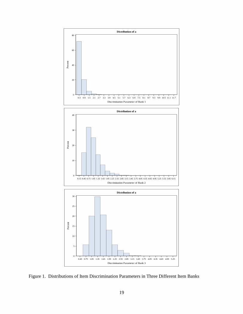
Table 2 summarizes the characteristics of the three item banks. The discrimination parameters ai

are generated from lowest values for item bank 1 to the highest values for bank 3. There are 2000 items

in each bank, and 1500 items are dichotomous items and 500 item s are polytomous items. Among 500

polytomous items, 250 are three category items and 250 are four category items. In terms of content

distribution, there are four sub-contents among all items. Regardless of item type, the distribution of

sub-content is uniform distribution of all items. Figure 1 depicts the distributions of item discrimination

parameters ai in three different item banks.

4. CAT Design

The CAT employs a fixed test length design with the target test length of 40 items. The

maximum test length could be 43 and the 3 extra items are used for the sub-content(s) that has largest

standard error of measurement (SEM). Each test cover four sub-contents with 20% of items for each

sub-content areas.

5. Method for Selecting the First Item

In this study, the first item for any given examinee has a difficulty value of 0.5 logit lower than

examinee’s true ability. The true ability for the first item is simulated with mean of standard normal

7

distribution.

6. Ability Estimation Method

The ability estimation method used is a combination of the EAP and the MLE methods. The

EAP method provides provisional ability estimation to select items and the MLE method provides the

final estimates. The person ability is simulated based on standard normal distributions.

7. Item Selection Method

Item selection methods used in this study are sequential. This means the selection is in

a hierarchical order based on item information with sub-content constraints. There are three information

zone sizes (another independent variable) of the item information in equations (4) and (6) for different

selection tiers. All item selection of different research designs follows the same steps with three tiers:

Tier 1. Selecting a group of 5 items from the item bank based on information zone size one, then

selecting one item randomly from a group items. If none item can be found, then go to tier 2.

Tier 2. Selecting a group of 5 items from the item bank based on information zone size two, then

selecting one item randomly from a group items. If none item can be found, then go to tier 3.

Tier 3. Selecting an item that have the best (by sorting) values in tier 2.

The size of item information is determined by the absolute distance (zone) infˆ in logit

between provisional ability estimation ̂ and theta inf to calculate the candidate items information.

There are three information zone sizes for tier 1 and 2 selection.

Tier1. Small zone size 1.0înf ;

Median zone size 3.0înf ;

Large zone size 5.0înf ;

Tier2. Small zone size 2.0înf ;

Median size 4.0înf ;

Large size 6.0înf ;

All three tiers use randomization strategy (McBride & Martin, 1983; Kingsbury & Zara, 1989) to

control for item exposure by randomly selecting an item from a given group of items mentioned above.

8

In addition to the information criterion, the additional constraint is set on the content balance (Kingsbury

& Zara, 1991) for sub-content. In tier 3, if there is no item required for the sub-content, then the item

selection will drop this constraint requirement. This guarantees that the test will not stop with a content

proportion deviating from the test specification.

All simulations and statistical analyses are conducted by using SAS (SAS Institute Inc. 2013).

9

Results

The major objectives of this study are the effect of ignoring item discrimination parameters in

item selection on the accuracy of estimation of person parameters in CAT under given conditions of

item banks and test content coverage for matching the test specification.

1. Accuracy of Ability Estimation of Test

For a fixed-length CAT, the efficiency is embodied within the accuracy of examinee’s ability

estimation compared to a linear test. In this study, the conditional accuracies of examinees’ ability

estimation at each of true ability levels are expressed in terms of bias, SE, and RMSE under different

simulation conditions. Table 3 presents the average accuracy of conditional ability estimation across

information type (GPCM, PCM_U, PCM_C), information zone size (small, median, large), and item

bank (low, median, high). Figure 2 to 4 depicts the conditional accuracy of ability estimation in terms of

bias, SE, and RMSE under three different item information zone sizes.

First, across three information zone sizes, the item information type has some impact on ability

estimation accuracy indexes bias, SE, and RMSE along ability range (theta from -3 to 3) for the bank

with low ai discrimination parameters. The item information type has a slight impact on ability

estimation accuracy indexes SE and RMSE at high ability range (theta>2) for the banks with median and

high ai discrimination parameters. Second, across the three information zone sizes, it seems that the

small information zone has large differences of ability estimation over the three information types. The

bias difference among the three information types is small and the difference of SE and RMSE of the

three information types are inconsistent across item bank and information zone sizes. However, in the

high ability range, in general, the information from GPCM seems to be better than both the information

of PCM_U and PCM_C. The results for the accuracy of the conditional ability estimation indicate that

an item bank with higher ai discrimination parameters has a better estimation than the bank that with

lower ai discrimination parameters. However, the difference is larger over different information types

from the item bank with either high or low discrimination parameter than that from the item bank with

median discrimination parameters.

2. Content Coverage

Content coverage measures how well the test meets the test specification and content constraints

specified in this study.

10

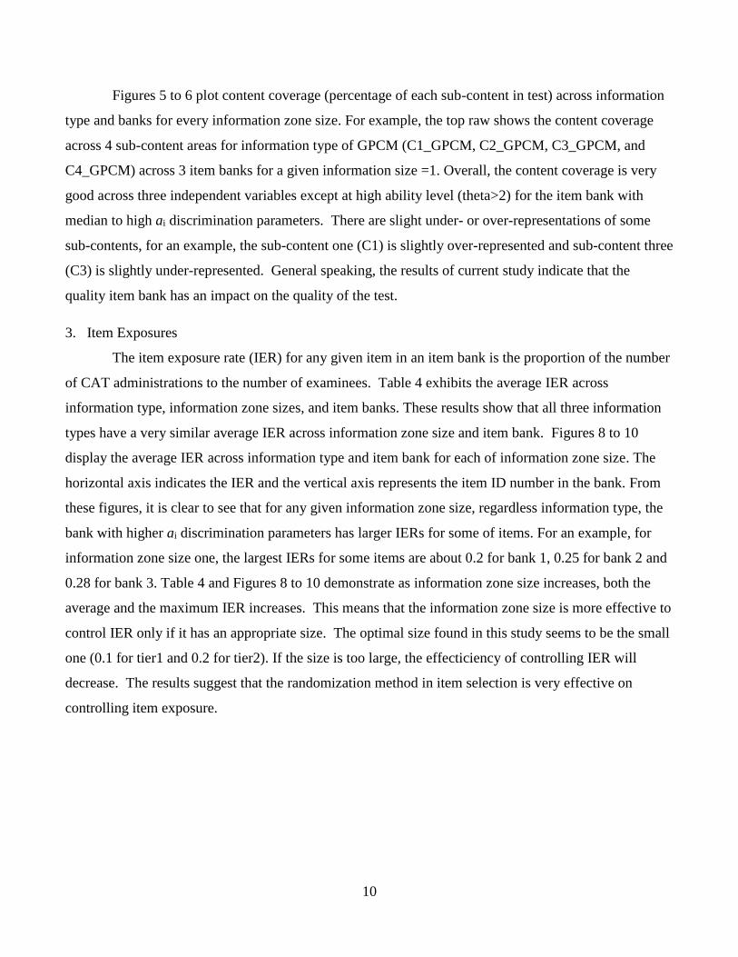
Figures 5 to 6 plot content coverage (percentage of each sub-content in test) across information

type and banks for every information zone size. For example, the top raw shows the content coverage

across 4 sub-content areas for information type of GPCM (C1_GPCM, C2_GPCM, C3_GPCM, and

C4_GPCM) across 3 item banks for a given information size =1. Overall, the content coverage is very

good across three independent variables except at high ability level (theta>2) for the item bank with

median to high ai discrimination parameters. There are slight under- or over-representations of some

sub-contents, for an example, the sub-content one (C1) is slightly over-represented and sub-content three

(C3) is slightly under-represented. General speaking, the results of current study indicate that the

quality item bank has an impact on the quality of the test.

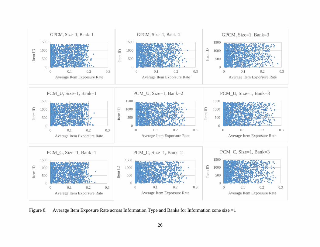
3. Item Exposures

The item exposure rate (IER) for any given item in an item bank is the proportion of the number

of CAT administrations to the number of examinees. Table 4 exhibits the average IER across

information type, information zone sizes, and item banks. These results show that all three information

types have a very similar average IER across information zone size and item bank. Figures 8 to 10

display the average IER across information type and item bank for each of information zone size. The

horizontal axis indicates the IER and the vertical axis represents the item ID number in the bank. From

these figures, it is clear to see that for any given information zone size, regardless information type, the

bank with higher ai discrimination parameters has larger IERs for some of items. For an example, for

information zone size one, the largest IERs for some items are about 0.2 for bank 1, 0.25 for bank 2 and

0.28 for bank 3. Table 4 and Figures 8 to 10 demonstrate as information zone size increases, both the

average and the maximum IER increases. This means that the information zone size is more effective to

control IER only if it has an appropriate size. The optimal size found in this study seems to be the small

one (0.1 for tier1 and 0.2 for tier2). If the size is too large, the effecticiency of controlling IER will

decrease. The results suggest that the randomization method in item selection is very effective on

controlling item exposure.

11

Discussion and Conclusions

Because item information plays such an important role in today’s large-scale, high-stakes CAT

assessments in K-12 education, the impact on test scores must be explored and evidence must be

provided for any modifications about item information equation. The major purpose of this study is to

examine the impact of using approximation of information on student scores and to verify on the claims

made by test vendors. The most important independent variable in this study is information type that includes

original IRT model GPCM information, and two approximated information (PCM_U and PCM_C

information). The reason for using two approximate information is lack of detailed information on the

modification or approximation of the GPCM information. We are confident that SBAC could employ either

of these two approximated information. The second important independent variable in this study is item

bank; because we do not have the access to the SBAC operational item banks, but simulated item banks

instead. How closely our simulated item bank is to SBAC is not clear even though we attempted to target the

distribution of SBAC item parameters.

The results from this study show that information type has certain effects on the accuracy of ability

estimation at conditional theta level. This is especially true for the item bank with low discrimination

parameters (Bank 1). For example, the left-top rows plots in figures 2 to 3 show that at the high ability level

(theta>0), the biases are under-estimated (bias has negative value). On the contrary, the MLE is usually over-

estimated ability at high ability level for normal item parameters. The direction of biases for item banks with

median and high discrimination parameters (banks 2 and 3) are no longer “bent-down” by low discrimination

parameters. Although the difference of bias across item information type for different information zone size

and item bank is negligible, the differences of SE and RMSE across information type and information zone

sizes are very noticeable for banks (bank 1 and 3) with both low and high item discrimination parameters.

Such as obvious differences indicate that the item bank contains a large portion of items that have either low

or high discrimination parameters, replacing the original item information (information based IRT model

used to calibrate items) with approximated information will have impact on the accuracy of ability

estimation. When the item bank contains a large proportion item with median discrimination values, such as

ai values are close to 1, then the impact of using approximated information could be negligible. This is

because when ai values are close to 1, the information equations (4) and (6) based on the GPCM is close

to the information based on Rasch and PCM. Then, the future research questions could be if most

calibrated items in the item bank have ai values close to 1, if there are any advantages using the

12

2PL/GPCM over Rasch/PCM? Is it true to choose the 2PL/GPCM over Rasch/PCM because

2PL/GPCM can model higher discrimination parameters?

The second finding in this study is that information type has no impact on content recovery

across information zone size and item banks because content constraints built-in for item selection is

fixed and the information type is unlikely to have an impact on content recovery, unless the item bank

size is extremely small or the distribution of item content in the bank is out of balance.

The last finding from this study is on IER. One of rationale claimed by the test vendor to use

approximate information instead of using original information is to treat discrimination parameters as a

constant to eliminate bias and help equalize exposure. The results (Table 4) from this study did not find

evidence to support such claim. However, this could be because two different item exposure control methods

are used in the process for item selection. This study shows that other factors such as information zone size

has more of an impact on IER than information type. In general, the randomization method in item

selection in this study is very effective on controlling item exposure.

Educational Importance of the Study

Item information in CAT has a significant impact on the item selection and quality of scoring student

in educational and psychological tests, and the accuracy of scoring in CAT affects educational selection,

classification, and evaluation decisions at individual student and group levels. When sub-content scores are

reported at the individual student level, such as SBAC assessments, the quality of scoring is critical due to

limited number of items. The choice of item information function is usually consistent with selected IRT

model in CAT. Using approximated information in item selection in CAT will lead to differences in the

accuracy of ability estimation and item exposure. It is also fund that other factors, such as quality of item

bank, item selection method, etc. may contribute the difference as well.

13

References

Birnbaum, A. (1968). Some latent ability models and their use in inferring an examinee’s ability. In F.

M. Lord & M. R. Novick, Statistical theories of mental test scores. Reading MA: Addison-

Wesley.

Bock, R. D., & Aitken, M. (1981). Marginal maximum likelihood estimation of item parameters:

Application of an EM algorithm. Psychomtrika, 46, 443-459.

Bock, R. D., & Mislevy, R. J. (1982). Adaptive EAP estimation of ability in a microcomputer

environment. Applied Psychological Measurement, 6, 431-444.

Bradlow, E. T. (1996). Negative information and the three-parameter logistic model. Journal of

Educational and Behavioral Statistics, 21, 179–185. doi:10.2307/1165216

Cheng, Y., & Chang, H. (2009). The maximum priority index method for severely constrained item

selection in computerized adaptive testing. British Journal of Mathematical and Statistical

Psychology, 63, 369-383

Cohen, J. & Albright, L. (2014). Smarter Balanced adaptive item selection algorithm design report.

Retrieved from http://www.smarterapp.org/specs/AdaptiveAlgorithm.html

Dodd, B. G., De Ayala, R. J., & Koch, W. R. (1995). Computerized adaptive testing with polytomous

items. Applied Psychological Measurement, 19, 5-22.

Kingsbury, G. G., & Zara, A. R. (1989). Procedures for selecting items for computerized adaptive tests.

Applied Measurement in Education, 2, 359–375.

Kingsbury, G. G., & Zara, A. (1991). A comparison of procedures for content-sensitive item

selection in computerized adaptive testing. Applied Measurement in Education, 4, 241–261.

Lord, F. M., & Novick, M. R. (1968). Statistical theories of mental test scores. Reading, MA: Addison-

Wesley

Magis, D. (2015). A Note on the Equivalence Between Observed and Expected Information Functions

With Polytomous IRT Models. Journal of Educational and Behavioral Statistics, Vol. 40, No. 1,

pp. 96–105.

Masters, G.N. (1982). A Rasch model for partial credit scoring. Psychometrika, 47, 149-174.

McBride, J. R., & Martin, J. T. (1983). Reliability and validity of adaptive ability tests in a military

setting. In D. J. Weiss (Ed.), New horizons in testing: Latent trait test theory and computerized

adaptive testing (pp.224-236). New York: Academic Press.

Muraki, E. (1992). A Generalized Partial Credit Model: Application of an EM algorithm. Applied

Psychological Measurement, 16(2): 159–176.

http://www.smarterapp.org/specs/AdaptiveAlgorithm.html

14

Samejima, F. (1969). Estimation of latent ability using a response pattern of graded scores.

Psychomtrika monograph, No. 17.

Samejima, F. (1973). A comment to Birnbaum’s three-parameter logistic model in the latent trait theory.

Psychometrika, 38, 221–233. doi:10.1007/BF02291115

Samejima, F. (1994). Some critical observations of the test information function as a measure of local

accuracy in ability estimation. Psychometrika, 59, 307–329. doi:10.1007/BF02296127

SAS Institute Inc. (2013). SAS® 9.4 Guide to Software. Updates. Cary, NC: SAS Institute Inc.

Shin, C., Chien, Y., Way, W. D., & Swanson, L. (2009). Weighted penalty model for content balancing

in CATs. Pearson. Retrieved from

http://www.pearsonedmeasurement.com/downloads/research/Weighted%20Penalty%20Mod

el.pdf.

Smarter Balanced Assessment Consortium (2016). Smarter Balanced Assessment Consortium: 2014-15

Technical Report. Retrieved from https://portal.smarterbalanced.org/library/en/2014-15-

technical-report.pdf

Stocking, M. L., & Swanson, L. (1993). A method for severely constrained item selection in adaptive

testing. Applied Psychological Measurement, 17, 277-292.

Stocking, M. L., Ward, W. C., & Potenza, M. T. (1998). Simulating the use of disclosed items in

computerized adaptive testing. Journal of Educational Measurement, 35, 46-68.

van der Linden, W. J. (1998). Bayesian item selection criteria for adaptive testing, Psychometrika, 2,

201-216.

van der Linden, W. J., & Pashley, P. J. (2000). Item selection and ability estimation in adaptive testing.

In W. J. vander Linder & C. A. W. Glas (Eds.), Computerized adaptive testing: Theory and

practice (pp. 1-25). Boston: Kluwer Academic.

van der Linden, W. J., & Reese, L. (1998). A model for optimal constrained adaptive testing. Applied

Psychological Measurement, 22 (3), 259-270.

Veerkamp, W. J. J. (1996). Statistical inference for adaptive testing. Internal report. Enschede, The

Netherlands: University of Twente.

Wainer, H., Dorans, N., Eignor, D., Flaugher, R., Green, B.F., Mislevy, R.J. and Steinberg, L. (2000).

Computerized adaptive testing: A primer (2nd ed.). Mahwah, NJ: Erlbaum.

Warm, T. A. (1989). Weighted likelihood estimation of ability in the item response theory.

Psychometrika, 54, 427-450.

Yen, W. M., Burket, G. R., & Sykes, R. C. (1991). Nonunique solutions to the likelihood equation for

the three-parameter logistic model. Psychometrika, 56, 39–54. doi:10. 1007/BF02294584

15

Table 1. Plan of Research Design

Dependent Variable Independent Variable

Average Conditional Index Information Type Information zone size Bank*

Bias GPCM, PCM_U, PCM_C Small, Median, Large 1,2,3

SE GPCM, PCM_U, PCM_C Small, Median, Large 1,2,3

RMSE GPCM, PCM_U, PCM_C Small, Median, Large 1,2,3

Content recovery GPCM, PCM_U, PCM_C Small, Median, Large 1,2,3

Item Exposure Rate GPCM, PCM_U, PCM_C Small, Median, Large 1,2,3

*: 1, 2, 3 – low, median, high discrimination parameters

16

Table 2. Item Characteristic in Item Bank

Bank Number of Category Number of Item Item Parameter Distributions

ai ~exp(x), xi~N(, 2) bi~N(, 2) ti1 ~U(l, h) ti2~U(l, h) ti3~U(l, h)

1 2 1500 =0.5, 2=0.2 =0, 2=1.2

3 250 =0.5, 2=0.2 =0, 2=1.0 l=-2.0, h=2.0 -ti1

4 250 =0.5, 2=0.2 =0, 2=1.0 -(ti2+-ti3) l=-1.0, h=0 l=0, h=1.0

2 2 1500 =1.0, 2=0.2 =0, 2=1.2

3 250 =1.0, 2=0.2 =0, 2=1.0 l=-2.0, h=2.0 -ti1

4 250 =1.0, 2=0.2 =0, 2=1.0 -(ti2+-ti3) l=-1.0, h=0 l=0, h=1.0

3 2 1500 =1.5, 2=0.2 =0, 2=1.2

3 250 =1.5, 2=0.2 =0, 2=1.0 l=-2.0, h=2.0 -ti1

4 250 =1.5, 2=0.2 =0, 2=1.0 -(ti2+-ti3) l=-1.0, h=0 l=0, h=1.0

17

Table 3. Average Accuracy of Conditional Person Estimation across Information Type,

Information zone size, and Item Bank.

Theta

Statistics Based on Different Information Function

Size Bank GPCM PCM_U PCM_C GPCM PCM_U PCM_C GPCM PCM_U PCM_C

Bias Bias Bias SE SE SE RMSE RMSE RMSE

Small 1 -3 0.56 0.26 0.58 2.90 2.30 3.14 2.95 2.32 3.19

-2 0.34 0.53 0.53 2.17 3.03 3.04 2.20 3.08 3.08 -1 0.26 0.18 0.21 2.07 2.27 2.07 2.08 2.28 2.08

-0.5 0.23 0.03 0.22 2.23 1.79 2.14 2.24 1.79 2.15

0 0.18 0.06 0.08 2.07 1.52 2.33 2.08 1.52 2.33 1 -0.80 -0.38 -0.22 2.61 2.89 2.95 2.73 2.91 2.96

2 -1.04 -1.00 -0.89 3.02 3.33 2.65 3.19 3.48 2.79

3 -1.62 -1.47 -1.66 4.21 3.86 3.64 4.51 4.13 4.00

2 -3 0.00 0.00 0.00 0.41 0.38 0.37 0.41 0.38 0.37

-2 0.05 0.05 0.05 0.39 0.34 0.38 0.39 0.35 0.38 -1 0.07 0.02 0.00 0.40 0.41 0.40 0.41 0.41 0.40

-0.5 0.07 0.02 -0.02 0.46 0.44 0.44 0.46 0.44 0.44

0 0.04 0.00 0.00 0.43 0.43 0.39 0.44 0.43 0.39 1 -0.05 0.01 0.02 0.53 0.56 0.55 0.53 0.56 0.55

2 0.09 0.11 0.07 0.72 0.75 0.80 0.73 0.76 0.81

3 0.36 0.14 0.10 1.52 1.24 0.90 1.56 1.25 0.91

3 -3 -0.02 -0.01 0.01 0.27 0.24 0.25 0.27 0.24 0.26

-2 0.01 0.01 0.02 0.28 0.28 0.27 0.28 0.28 0.27 -1 0.01 0.01 -0.01 0.29 0.31 0.30 0.29 0.31 0.30

-0.5 0.01 0.04 -0.01 0.31 0.34 0.32 0.31 0.34 0.32

0 0.02 -0.01 -0.05 0.36 0.33 0.35 0.36 0.33 0.35 1 0.04 0.01 -0.01 0.44 0.43 0.45 0.44 0.43 0.45

2 0.06 0.07 -0.04 1.05 1.07 0.53 1.05 1.07 0.53

3 -0.04 -0.35 -0.22 1.98 0.41 1.30 1.98 0.54 1.31

Median 1 -3 0.57 0.19 0.59 3.15 1.92 3.13 3.20 1.93 3.19

-2 0.23 0.41 0.48 1.85 2.75 2.75 1.86 2.78 2.79 -1 0.17 0.12 -0.10 1.86 1.34 1.33 1.87 1.35 1.33

-0.5 0.22 0.01 0.02 2.00 2.44 2.53 2.01 2.44 2.53

0 -0.32 0.32 -0.36 2.13 2.57 2.87 2.16 2.58 2.90 1 -0.68 -0.98 -0.53 2.28 2.92 2.59 2.38 3.08 2.65

2 -1.33 -1.30 -0.91 3.14 3.16 2.70 3.41 3.41 2.85

3 -1.46 -1.26 -1.41 3.66 3.37 3.96 3.94 3.59 4.20

2 -3 -0.02 0.01 -0.02 0.39 0.39 0.35 0.39 0.39 0.35

-2 0.02 0.05 0.05 0.38 0.33 0.38 0.38 0.33 0.38 -1 0.00 0.00 -0.03 0.44 0.40 0.41 0.44 0.40 0.41

-0.5 -0.01 0.04 0.05 0.45 0.43 0.44 0.45 0.43 0.44

0 0.03 0.04 0.04 0.44 0.42 0.43 0.44 0.42 0.43 1 0.08 0.15 0.03 0.67 0.64 0.56 0.67 0.66 0.56

2 0.05 0.05 0.08 0.74 0.69 0.72 0.74 0.69 0.72

3 0.03 0.00 0.14 0.87 0.88 0.96 0.87 0.88 0.97

3 -3 0.02 0.00 0.00 0.26 0.27 0.27 0.26 0.27 0.27 -2 0.02 0.02 0.02 0.27 0.26 0.26 0.27 0.26 0.26

-1 0.01 -0.02 -0.03 0.28 0.31 0.31 0.28 0.31 0.32

-0.5 0.02 -0.01 -0.02 0.33 0.29 0.30 0.33 0.29 0.30 0 0.02 -0.04 -0.05 0.34 0.34 0.34 0.34 0.34 0.35

1 0.03 0.06 0.05 0.47 0.45 0.47 0.47 0.45 0.47

2 -0.03 0.12 0.00 0.54 1.06 0.50 0.54 1.07 0.50 3 -0.13 -0.07 -0.19 1.77 1.97 1.57 1.78 1.98 1.58

Large 1 -3 0.27 0.65 0.67 2.32 3.12 3.60 2.34 3.19 3.66

-2 0.70 0.10 0.07 3.44 1.38 1.52 3.51 1.39 1.52

-1 0.60 -0.03 0.04 2.89 0.77 2.08 2.96 0.77 2.08 -0.5 0.26 -0.06 -0.10 2.42 2.06 1.06 2.43 2.07 1.07

0 0.00 0.24 -0.10 1.94 2.79 2.24 1.94 2.80 2.25

1 -0.32 -0.32 -0.61 2.70 2.70 2.47 2.72 2.72 2.55 2 -1.14 -1.17 -1.15 3.54 3.63 2.65 3.72 3.81 2.88

18

3 -1.97 -1.90 -1.53 4.62 4.56 4.45 5.02 4.94 4.70

2 -3 0.01 0.00 -0.01 0.39 0.38 0.33 0.39 0.38 0.33 -2 0.03 0.03 0.04 0.36 0.39 0.36 0.36 0.39 0.36

-1 0.00 0.06 0.02 0.39 0.41 0.41 0.39 0.42 0.41

-0.5 0.02 0.04 0.04 0.41 0.42 0.42 0.41 0.42 0.42 0 0.00 -0.03 0.02 0.49 0.42 0.45 0.49 0.42 0.45

1 0.02 0.04 0.05 0.61 0.59 0.56 0.61 0.59 0.56

2 0.09 -0.01 0.08 0.80 0.85 0.73 0.80 0.85 0.73 3 0.22 0.15 0.14 1.28 0.97 1.24 1.30 0.98 1.25

3 -3 0.00 0.01 -0.01 0.28 0.27 0.29 0.28 0.27 0.29 -2 0.03 0.01 0.02 0.28 0.27 0.29 0.28 0.27 0.29

-1 0.01 0.02 0.04 0.33 0.30 0.32 0.33 0.30 0.32

-0.5 0.00 0.02 0.05 0.31 0.35 0.32 0.31 0.35 0.32 0 0.02 0.01 -0.02 0.35 0.37 0.34 0.35 0.37 0.34

1 0.04 0.03 0.03 0.50 0.48 0.44 0.50 0.48 0.44

2 0.02 0.00 0.11 0.53 0.50 1.04 0.53 0.50 1.05 3 -0.07 -0.14 -0.12 2.34 1.99 1.99 2.34 2.00 1.99

Table 4. Average Item Exposure Rate across Information Type, Information zone size, and Item

Bank.

Information zone

size Item Bank*

Average Item Exposure

GPCM PCM_U PCUM_C

Small 1 0.074 0.074 0.074

2 0.070 0.071 0.071

3 0.070 0.071 0.070

Median 1 0.075 0.075 0.075

2 0.072 0.073 0.072

3 0.071 0.071 0.071

Large 1 0.076 0.076 0.075

2 0.073 0.074 0.072

3 0.072 0.072 0.071

*: 1, 2, 3 – low, median, high discrimination parameters

19

Figure 1. Distributions of Item Discrimination Parameters in Three Different Item Banks

0.3 0.9 1.5 2.1 2.7 3.3 3.9 4.5 5.1 5.7 6.3 6.9 7.5 8.1 8.7 9.3 9.9 10.5 11.1 11.7

Discrimination Parameter of Bank 1

0

20

40

60

80

Per

cent

Distribution of a

0.15 0.45 0.75 1.05 1.35 1.65 1.95 2.25 2.55 2.85 3.15 3.45 3.75 4.05 4.35 4.65 4.95 5.25 5.55 5.85 6.15


0

10

20

30

40

Per

cent

Distribution of a

0.45 0.75 1.05 1.35 1.65 1.95 2.25 2.55 2.85 3.15 3.45 3.75 4.05 4.35 4.65 4.95 5.25


0

5

10

15

20

25

30

Per

cent

Distribution of a

20

Figure 2. Average Conditional Bias, SE, and RMSE across Information Type and Banks for Information zone size=1

-2.0

-1.0

0.0

1.0

2.0

-3.0 -2.0 -1.0 0.0 1.0 2.0 3.0

Bia

s

Theta

Bias (Size=1, Bank=1)

Bias_GPCMBias_PCM_UBias_PCM_C

-2.0

-1.0

0.0

1.0

2.0

-3.0 -2.0 -1.0 0.0 1.0 2.0 3.0

Bia

s

Theta



-2.0

-1.0

0.0

1.0

2.0

-3.0 -2.0 -1.0 0.0 1.0 2.0 3.0

Bia

s

Theta



0.0

1.0

2.0

3.0

4.0

5.0

-3.0 -2.0 -1.0 0.0 1.0 2.0 3.0

SE

Theta

SE (Size=1, Bank=1)

SE_GPCM

SE_PCM_U

SE_PCM_C 0.0

1.0

2.0

3.0

4.0

5.0

-3.0 -2.0 -1.0 0.0 1.0 2.0 3.0

SE

Theta

SE (Size=1, Bank=2)

SE_GPCM

SE_PCM_U

SE_PCM_C

0.0

1.0

2.0

3.0

4.0

5.0

-3.0 -2.0 -1.0 0.0 1.0 2.0 3.0

SE

Theta

SE (Size=1, Bank=3)

SE_GPCMSE_PCM_USE_PCM_C

0.0

1.0

2.0

3.0

4.0

5.0

-3.0 -2.0 -1.0 0.0 1.0 2.0 3.0

RM

SE

Theta

RMSE (Size=1, Bank=1)

RMSE_GPCM

RMSE_PCM_U

RMSE_PCM_C

0.0

1.0

2.0

3.0

4.0

5.0

-3.0 -2.0 -1.0 0.0 1.0 2.0 3.0

RM

SE

Theta


RMSE_GPCMRMSE_PCM_URMSE_PCM_C

0.0

1.0

2.0

3.0

4.0

5.0

-3.0 -2.0 -1.0 0.0 1.0 2.0 3.0

RM

SE

Theta



21

Figure 3. Average Conditional Bias, SE, and RMSE across Information Type and Banks for Information zone size =2

-2.0

-1.0

0.0

1.0

2.0

-3.0 -2.0 -1.0 0.0 1.0 2.0 3.0

Bia

s

Theta

Bias (Size=2, Bank=1) Bias_GPCM

Bias_PCM_U

Bias_PCM_C

-2.0

-1.0

0.0

1.0

2.0

-3.0 -2.0 -1.0 0.0 1.0 2.0 3.0

Bia

s

Theta


Bias_GPCM

Bias_PCM_U

Bias_PCM_C-2.0

-1.0

0.0

1.0

2.0

-3.0 -2.0 -1.0 0.0 1.0 2.0 3.0

Bia

s

Theta


Bias_GPCM

Bias_PCM_U

Bias_PCM_C

0.0

1.0

2.0

3.0

4.0

5.0

-3.0 -2.0 -1.0 0.0 1.0 2.0 3.0

SE

Theta

SE (Size=2, Bank=1)

SE_GPCMSE_PCM_USE_PCM_C

0.0

1.0

2.0

3.0

4.0

5.0

-3.0 -2.0 -1.0 0.0 1.0 2.0 3.0

SE

Theta

SE (Size=2, Bank=2)

SE_GPCM

SE_PCM_U

SE_PCM_C

0.0

1.0

2.0

3.0

4.0

5.0

-3.0 -2.0 -1.0 0.0 1.0 2.0 3.0

SE

Theta

SE (Size=2, Bank=3)

SE_GPCM

SE_PCM_U

SE_PCM_C

0.0

1.0

2.0

3.0

4.0

5.0

-3.0 -2.0 -1.0 0.0 1.0 2.0 3.0

RM

SE

Theta


RMSE_GPCM

RMSE_PCM_U

RMSE_PCM_C0.0

1.0

2.0

3.0

4.0

5.0

-3.0 -2.0 -1.0 0.0 1.0 2.0 3.0

RM

SE

Theta



0.0

1.0

2.0

3.0

4.0

5.0

-3.0 -2.0 -1.0 0.0 1.0 2.0 3.0

RM

SE

Theta



22

Figure 4. Average Conditional Bias, SE, and RMSE across Information Type and Banks for Information zone size =3

-2.0

-1.0

0.0

1.0

2.0

-3.0 -2.0 -1.0 0.0 1.0 2.0 3.0

Bia

s

Theta



-2.0

-1.0

0.0

1.0

2.0

-3.0 -2.0 -1.0 0.0 1.0 2.0 3.0

Bia

s

Theta


Bias_GPCM

Bias_PCM_U

Bias_PCM_C

-2.0

-1.0

0.0

1.0

2.0

-3.0 -2.0 -1.0 0.0 1.0 2.0 3.0

Bia

s

Theta


Bias_GPCM

Bias_PCM_U

Bias_PCM_C

0.0

1.0

2.0

3.0

4.0

5.0

-3.0 -2.0 -1.0 0.0 1.0 2.0 3.0

SE

Theta

SE (Size=3, Bank=1)

SE_GPCMSE_PCM_USE_PCM_C 0.0

1.0

2.0

3.0

4.0

5.0

-3.0 -2.0 -1.0 0.0 1.0 2.0 3.0

SE

Theta

SE (Size=3, Bank=2)

SE_GPCM

SE_PCM_U

SE_PCM_C

0.0

1.0

2.0

3.0

4.0

5.0

-3.0 -2.0 -1.0 0.0 1.0 2.0 3.0

SE

Theta

SE (Size=3, Bank=3)

SE_GPCM

SE_PCM_U

SE_PCM_C

0.0

1.0

2.0

3.0

4.0

5.0

-3.0 -2.0 -1.0 0.0 1.0 2.0 3.0

RM

SE

Theta


RMSE_GPCM

0.0

1.0

2.0

3.0

4.0

5.0

-3.0 -2.0 -1.0 0.0 1.0 2.0 3.0

RM

SE

Theta



0.0

1.0

2.0

3.0

4.0

5.0

-3.0 -2.0 -1.0 0.0 1.0 2.0 3.0

RM

SE

Theta



23

Figure 5. Content Coverage across Information Type and Banks for Information zone size =1

0.0

0.1

0.2

0.3

0.4

0.5

-3.0 -1.0 1.0 3.0

Per

centa

ge

Co

ver

age

Conditional Theta

Content Coverage (Size=1, Bank=1)

C1_GPCM C2_GPCM

C3_GPCM C4_GPCM

0.0

0.1

0.2

0.3

0.4

0.5

-3.0 -1.0 1.0 3.0

Per

centa

ge

Co

ver

age

Conditional Theta


C1_GPCM C2_GPCM

C3_GPCM C4_GPCM

0.0

0.1

0.2

0.3

0.4

0.5

-3.0 -1.0 1.0 3.0

Per

centa

ge

Co

ver

age

Conditional Theta


C1_GPCM C2_GPCM

C3_GPCM C4_GPCM

0.0

0.1

0.2

0.3

0.4

0.5

-3.0 -1.0 1.0 3.0

Per

centa

ge

Co

ver

age

Conditional Theta


C1_PCM_C C2_PCM_C

C3_PCM_C C4_PCM_C

0.0

0.1

0.2

0.3

0.4

0.5

-3.0 -1.0 1.0 3.0Per

centa

ge

Co

ver

age

Conditional Theta


C1_PCM_C C2_PCM_C

C3_PCM_C C4_PCM_C

0.0

0.1

0.2

0.3

0.4

0.5

-3.0 -1.0 1.0 3.0

Per

centa

ge

Co

ver

age

Conditional Theta


C1_PCM_C C2_PCM_C

C3_PCM_C C4_PCM_C

0.0

0.1

0.2

0.3

0.4

0.5

-3.0 -1.0 1.0 3.0

Per

centa

ge

Co

ver

age

Conditional Theta


C1_PCM_U C2_PCM_UC3_PCM_U C4_PCM_U

0.0

0.1

0.2

0.3

0.4

0.5

-3.0 -1.0 1.0 3.0

Per

centa

ge

Co

ver

age

Conditional Theta



0.0

0.1

0.2

0.3

0.4

0.5

-3.0 -1.0 1.0 3.0

Per

centa

ge

Co

ver

age

Conditional Theta


C1_PCM_U C2_PCM_U

C3_PCM_U C4_PCM_U

24


0.0

0.1

0.2

0.3

0.4

0.5

-3.0 -1.0 1.0 3.0

Per

centa

ge

Co

ver

age

Conditional Theta


C1_GPCM C2_GPCM

C3_GPCM C4_GPCM

0.0

0.1

0.2

0.3

0.4

0.5

-3.0 -1.0 1.0 3.0

Per

centa

ge

Co

ver

age

Conditional Theta


C1_GPCM C2_GPCMC3_GPCM C4_GPCM

0.0

0.1

0.2

0.3

0.4

0.5

-3.0 -1.0 1.0 3.0

Per

centa

ge

Co

ver

age

Conditional Theta


C1_GPCM C2_GPCMC3_GPCM C4_GPCM

0.0

0.1

0.2

0.3

0.4

0.5

-3.0 -1.0 1.0 3.0

Per

centa

ge

Co

ver

age

Conditional Theta


C1_PCM_C C2_PCM_C

C3_PCM_C C4_PCM_C

0.0

0.1

0.2

0.3

0.4

0.5

-3.0 -1.0 1.0 3.0

Per

centa

ge

Co

ver

age

Conditional Theta


C1_PCM_C C2_PCM_C

C3_PCM_C C4_PCM_C

0.0

0.1

0.2

0.3

0.4

0.5

-3.0 -1.0 1.0 3.0

Per

centa

ge

Co

ver

age

Conditional Theta


C1_PCM_C C2_PCM_C

C3_PCM_C C4_PCM_C

0.0

0.1

0.2

0.3

0.4

0.5

-3.0 -1.0 1.0 3.0

Per

centa

ge

Co

ver

age

Conditional Theta



0.0

0.1

0.2

0.3

0.4

0.5

-3.0 -1.0 1.0 3.0

Per

centa

ge

Co

ver

age

Conditional Theta



0.0

0.1

0.2

0.3

0.4

0.5

-3.0 -1.0 1.0 3.0

Per

centa

ge

Co

ver

age

Conditional Theta


C1_PCM_U C2_PCM_U

C3_PCM_U C4_PCM_U

25


0.0

0.1

0.2

0.3

0.4

0.5

-3.0 -1.0 1.0 3.0

Per

centa

ge

Co

ver

age

Conditional Theta


C1_GPCM C2_GPCM

C3_GPCM C4_GPCM

0.0

0.1

0.2

0.3

0.4

0.5

-3.0 -1.0 1.0 3.0

Per

centa

ge

Co

ver

age

Conditional Theta


C1_GPCM C2_GPCM

C3_GPCM C4_GPCM

0.0

0.1

0.2

0.3

0.4

0.5

-3.0 -1.0 1.0 3.0

Per

centa

ge

Co

ver

age

Conditional Theta


C1_GPCM C2_GPCM

C3_GPCM C4_GPCM

0.0

0.1

0.2

0.3

0.4

0.5

-3.0 -1.0 1.0 3.0

Per

centa

ge

Co

ver

age

Conditional Theta


C1_PCM_C C2_PCM_C

C3_PCM_C C4_PCM_C

0.0

0.1

0.2

0.3

0.4

0.5

-3.0 -1.0 1.0 3.0

Per

centa

ge

Co

ver

age

Conditional Theta


C1_PCM_C C2_PCM_C

C3_PCM_C C4_PCM_C

0.0

0.1

0.2

0.3

0.4

0.5

-3.0 -1.0 1.0 3.0

Per

centa

ge

Co

ver

age

Conditional Theta


C1_PCM_C C2_PCM_C

C3_PCM_C C4_PCM_C

0.0

0.1

0.2

0.3

0.4

0.5

-3.0 -1.0 1.0 3.0

Per

centa

ge

Co

ver

age

Conditional Theta



0.0

0.1

0.2

0.3

0.4

0.5

-3.0 -1.0 1.0 3.0

Per

centa

ge

Co

ver

age

Conditional Theta



0.0

0.1

0.2

0.3

0.4

0.5

-3.0 -1.0 1.0 3.0

Per

centa

ge

Co

ver

age

Conditional Theta


C1_PCM_U C2_PCM_U

C3_PCM_U C4_PCM_U

26

Figure 8. Average Item Exposure Rate across Information Type and Banks for Information zone size =1

0

500

1000

1500

0 0.1 0.2 0.3

Item

ID

Average Item Exporsure Rate

GPCM, Size=1, Bank=1

0

500

1000

1500

0 0.1 0.2 0.3

Item

ID



0

500

1000

1500

0 0.1 0.2 0.3

Item

ID



0

500

1000

1500

0 0.1 0.2 0.3

Item

ID


PCM_U, Size=1, Bank=1

0

500

1000

1500

0 0.1 0.2 0.3

Item

ID



0

500

1000

1500

0 0.1 0.2 0.3

Item

ID



0

500

1000

1500

0 0.1 0.2 0.3

Item

ID


PCM_C, Size=1, Bank=1

0

500

1000

1500

0 0.1 0.2 0.3

Item

ID



0

500

1000

1500

0 0.1 0.2 0.3

Item

ID



27


0

500

1000

1500

0 0.1 0.2 0.3

Item

ID



0

500

1000

1500

0 0.1 0.2 0.3

Item

ID



0

500

1000

1500

0 0.1 0.2 0.3

Item

ID



0

500

1000

1500

0 0.1 0.2 0.3

Item

ID



0

500

1000

1500

0 0.1 0.2 0.3

Item

ID



0

500

1000

1500

0 0.1 0.2 0.3

Item

ID



0

500

1000

1500

0 0.1 0.2 0.3

Item

ID



0

500

1000

1500

0 0.1 0.2 0.3

Item

ID



0

500

1000

1500

0 0.1 0.2 0.3

Item

ID



28


0

500

1000

1500

0 0.1 0.2 0.3

Item

ID



0

500

1000

1500

0 0.1 0.2 0.3

Item

ID



0

500

1000

1500

0 0.1 0.2 0.3

Item

ID



0

500

1000

1500

0 0.1 0.2 0.3

Item

ID



0

500

1000

1500

0 0.1 0.2 0.3

Item

ID



0

500

1000

1500

0 0.1 0.2 0.3

Item

ID



0

500

1000

1500

0 0.1 0.2 0.3

Item

ID



0

500

1000

1500

0 0.1 0.2 0.3

Item

ID



0

500

1000

1500

0 0.1 0.2 0.3

Item

ID



effects of ignoring discrimination parameter in cat item

Documents