animal-human discrimination track-level discrimination
TRANSCRIPT
Animal-Human Discrimination
Track-level Discrimination
Organization of Presentation
• Patterns of movement among non-human animals
• Home range concept
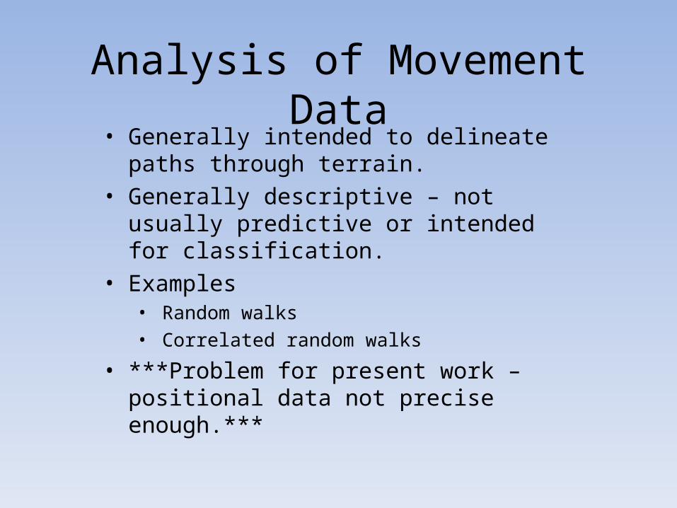
Analysis of Movement Data• Generally intended to delineate paths through
terrain.• Generally descriptive – not usually predictive
or intended for classification.• Examples
• Random walks• Correlated random walks
• ***Problem for present work – positional data not precise enough.***
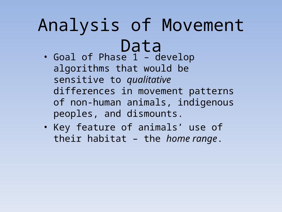
Analysis of Movement Data• Goal of Phase 1 – develop algorithms that
would be sensitive to qualitative differences in movement patterns of non-human animals, indigenous peoples, and dismounts.
• Key feature of animals’ use of their habitat – the home range.
Home Range Concept
• Territory = area that animal actively defends – by marking or actual physical combat
• Home range – area that an animal samples on a more-or-less regular basis.
• Home range may overlap with territories/home ranges of conspecifics.
• Habitat ‘quality’ is key determinant of home range size, location and utilization patterns
Home Range Concept
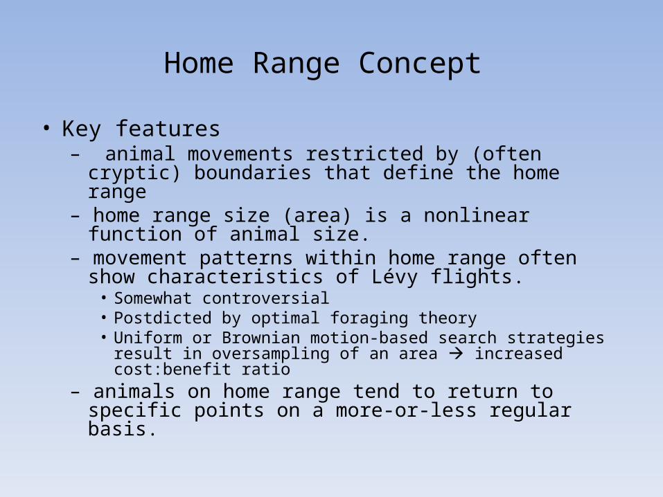
• Key features – animal movements restricted by (often cryptic) boundaries
that define the home range– home range size (area) is a nonlinear function of animal
size.– movement patterns within home range often show
characteristics of Lévy flights.• Somewhat controversial• Postdicted by optimal foraging theory• Uniform or Brownian motion-based search strategies result in
oversampling of an area increased cost:benefit ratio– animals on home range tend to return to specific points on
a more-or-less regular basis.
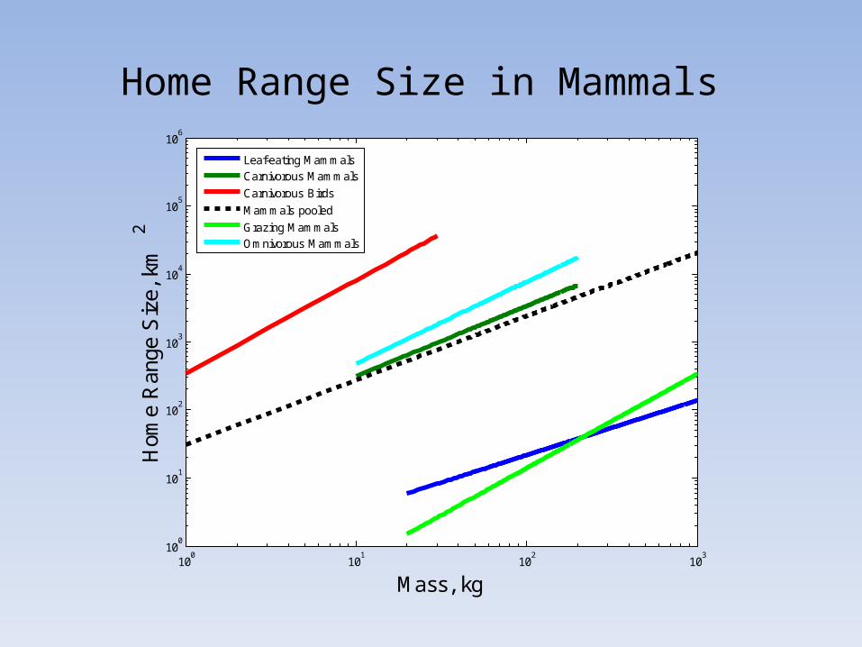
Home Range Size in Mammals
100
101
102
103
100
101
102
103
104
105
106
Mass, kg
Hom
e R
ange
Siz
e, k
m
2
Leaf-eating MammalsCarnivorous Mammals
Carnivorous Birds
Mammals pooled
Grazing MammalsOmnivorous Mammals
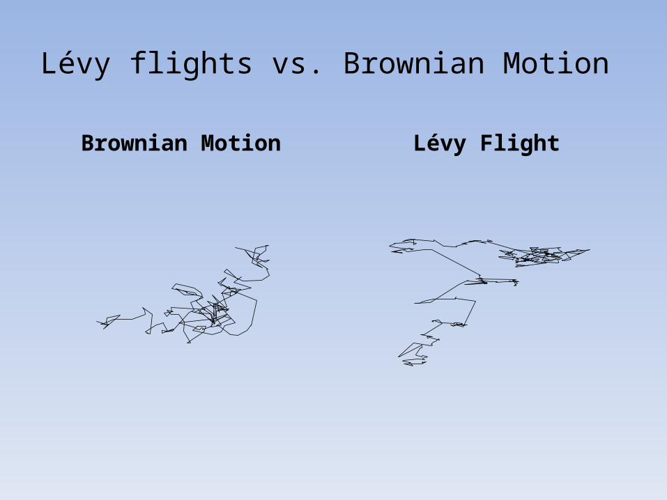
Lévy flights vs. Brownian Motion
Brownian Motion Lévy Flight
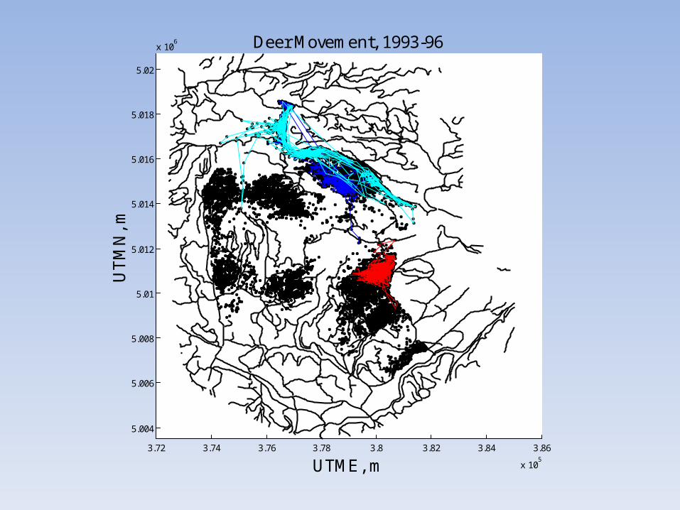
3.72 3.74 3.76 3.78 3.8 3.82 3.84 3.86
x 105
5.004
5.006
5.008
5.01
5.012
5.014
5.016
5.018
5.02
x 106 Deer Movement, 1993-96
UTME, m
UT
MN
, m
3.72 3.74 3.76 3.78 3.8 3.82 3.84 3.86
x 105
5.004
5.006
5.008
5.01
5.012
5.014
5.016
5.018
5.02
x 106 Elk Movement, 1993-96
UTME, m
UT
MN
, m
3.72 3.74 3.76 3.78 3.8 3.82 3.84 3.86
x 105
5.004
5.006
5.008
5.01
5.012
5.014
5.016
5.018
5.02
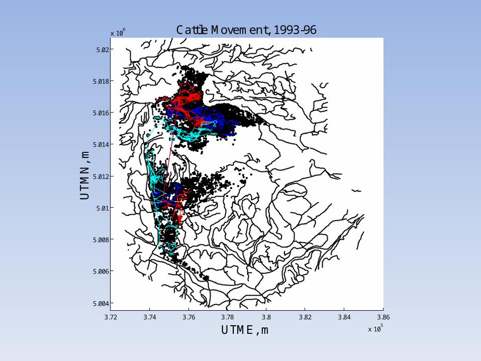
x 106 Cattle Movement, 1993-96
UTME, m
UT
MN
, m
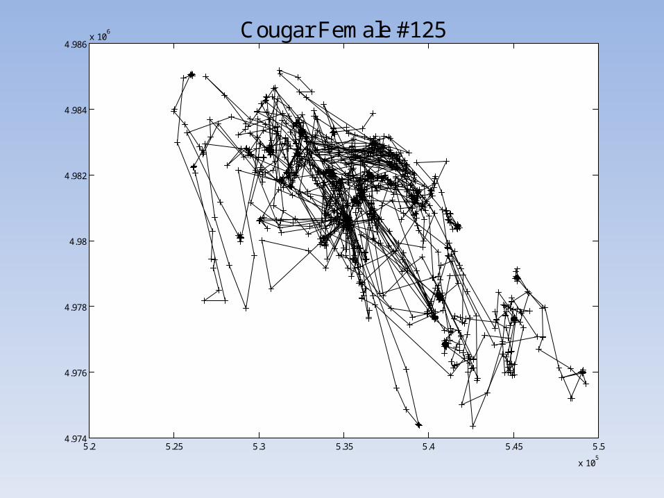
5.2 5.25 5.3 5.35 5.4 5.45 5.5
x 105
4.974
4.976
4.978
4.98
4.982
4.984
4.986x 10
6 Cougar Female #125
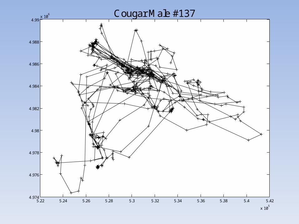
5.22 5.24 5.26 5.28 5.3 5.32 5.34 5.36 5.38 5.4 5.42
x 105
4.974
4.976
4.978
4.98
4.982
4.984
4.986
4.988
4.99x 10
6 Cougar Male #137
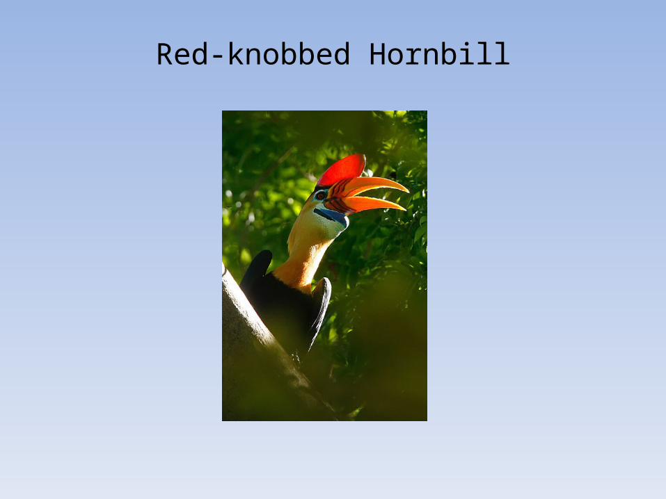
Red-knobbed Hornbill
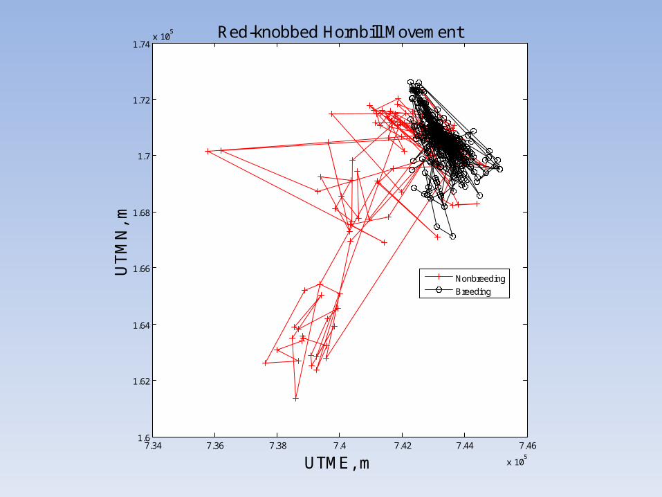
7.34 7.36 7.38 7.4 7.42 7.44 7.46
x 105
1.6
1.62
1.64
1.66
1.68
1.7
1.72
1.74x 10
5 Red-knobbed Hornbill Movement
UTME, m
UT
MN
, m
Nonbreeding
Breeding
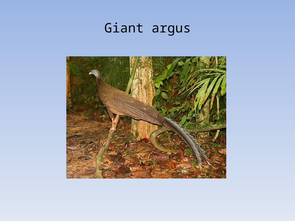
Giant argus
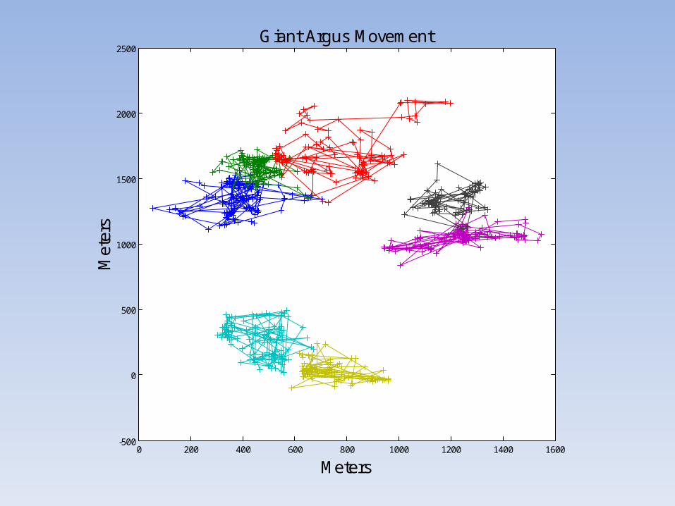
0 200 400 600 800 1000 1200 1400 1600-500
0
500
1000
1500
2000
2500
Meters
Met
ers
Giant Argus Movement
Analysis of Movement Data• We’re going to argue for a combined approach
based on a number of algorithms• My work so far – and for foreseeable future – is
aimed at producing an eclectic mix of algorithms that do the best job of meeting your needs.
Analysis of Movement Data
Wavelet Analysis(Discrete) Differential Geometry
Nonlinear algorithms
Analysis of Movement Data
Wavelet Analysis(Discrete) Differential Geometry
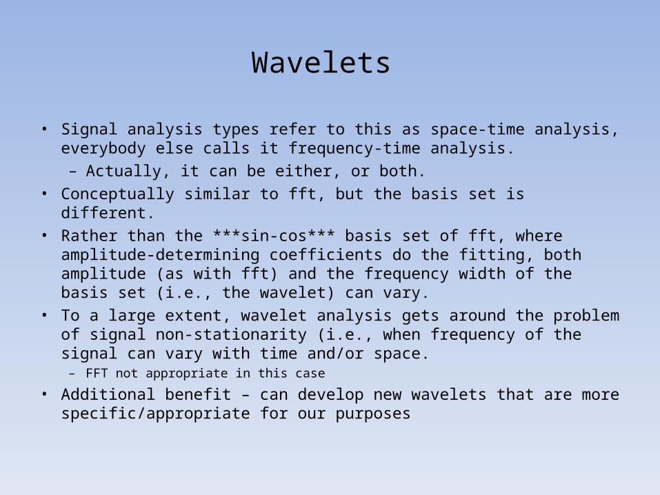
Wavelets
• Signal analysis types refer to this as space-time analysis, everybody else calls it frequency-time analysis. – Actually, it can be either, or both.
• Conceptually similar to fft, but the basis set is different.• Rather than the ***sin-cos*** basis set of fft, where amplitude-
determining coefficients do the fitting, both amplitude (as with fft) and the frequency width of the basis set (i.e., the wavelet) can vary.
• To a large extent, wavelet analysis gets around the problem of signal non-stationarity (i.e., when frequency of the signal can vary with time and/or space.
– FFT not appropriate in this case
• Additional benefit – can develop new wavelets that are more specific/appropriate for our purposes
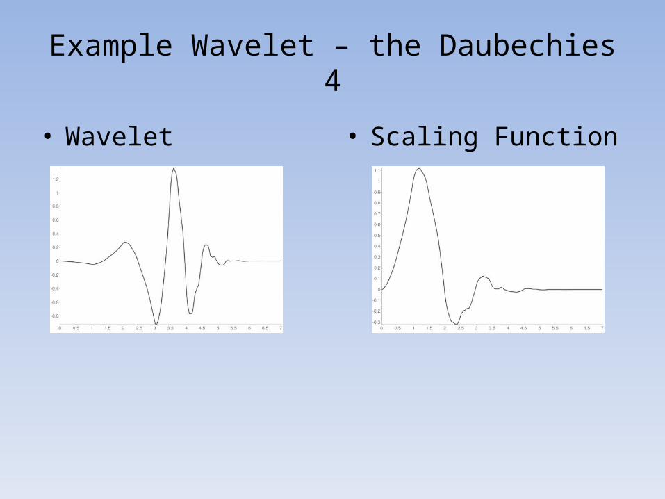
Example Wavelet – the Daubechies 4
• Wavelet • Scaling Function

x-axis 4.9 km
y-ax
is
6.7
km
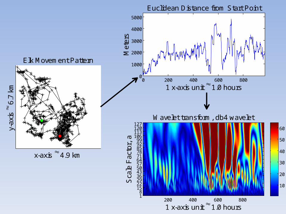
Elk Movement Pattern
0 200 400 600 8000
1000
2000
3000
4000
5000
1 x-axis unit 1.0 hours
Met
ers
Euclidean Distance from Start Point
Wavelet transform, db4 wavelet
1 x-axis unit 1.0 hours
Sca
le F
acto
r, a
200 400 600 800 1 8
15 22 29 36 43 50 57 64 71 78 85 92 99
106113120127
10
20
30
40
50
60
x-axis 24.3 km
y-ax
is
10.
8 km
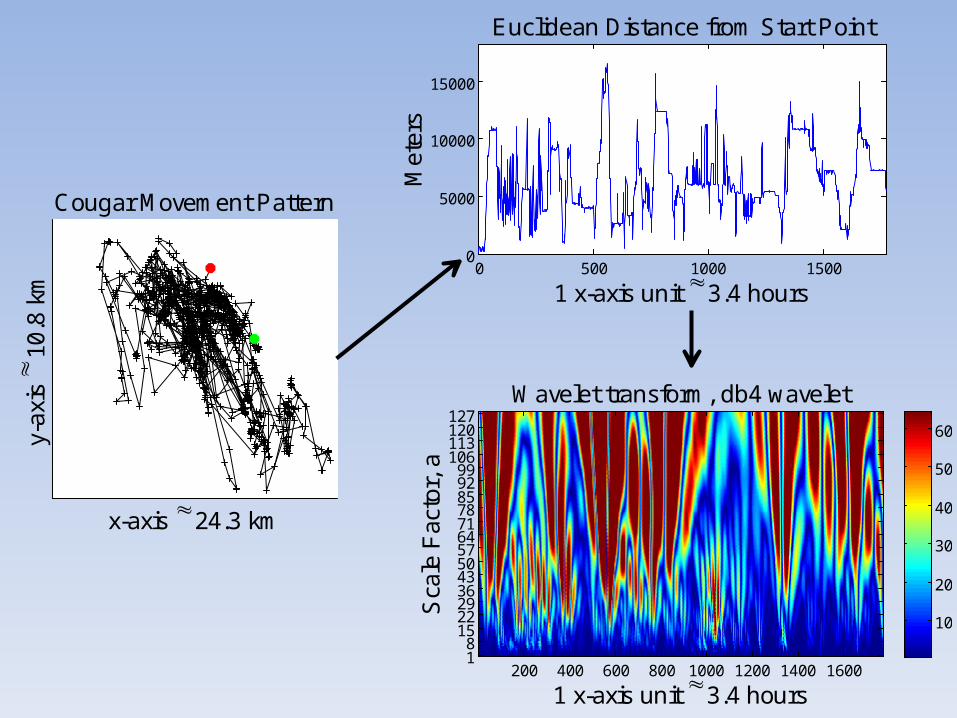
Cougar Movement Pattern
0 500 1000 15000
5000
10000
15000
1 x-axis unit 3.4 hours
Met
ers
Euclidean Distance from Start Point
Wavelet transform, db4 wavelet
1 x-axis unit 3.4 hours
Sca
le F
acto
r, a
200 400 600 800 1000 1200 1400 1600 1 8
15 22 29 36 43 50 57 64 71 78 85 92 99
106113120127
10
20
30
40
50
60
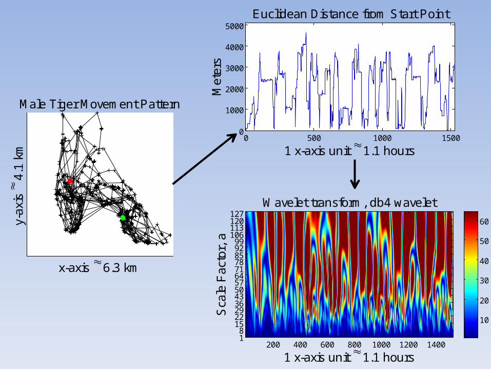
x-axis 6.3 km
y-ax
is
4.1
km
Male Tiger Movement Pattern
0 500 1000 15000
1000
2000
3000
4000
5000
1 x-axis unit 1.1 hours
Met
ers
Euclidean Distance from Start Point
Wavelet transform, db4 wavelet
1 x-axis unit 1.1 hours
Sca
le F
acto
r, a
200 400 600 800 1000 1200 1400 1 8
15 22 29 36 43 50 57 64 71 78 85 92 99
106113120127
10
20
30
40
50
60
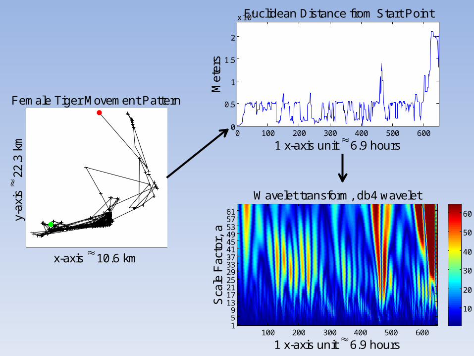
Female Tiger Movement Pattern
x-axis 10.6 km
y-ax
is
22.
3 km
0 100 200 300 400 500 6000
0.5
1
1.5
2
x 104
1 x-axis unit 6.9 hours
Met
ers
Euclidean Distance from Start Point
Wavelet transform, db4 wavelet
1 x-axis unit 6.9 hours
Sca
le F
acto
r, a
100 200 300 400 500 600 1 5 9
13172125293337414549535761
10
20
30
40
50
60
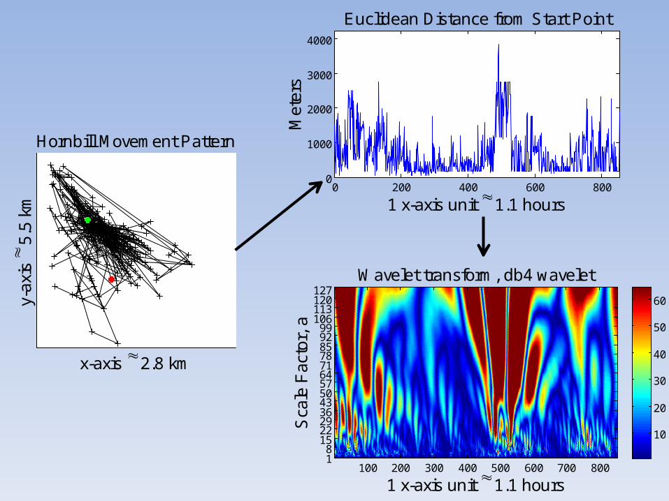
x-axis 2.8 km
y-ax
is
5.5
km
Hornbill Movement Pattern
0 200 400 600 8000
1000
2000
3000
4000
1 x-axis unit 1.1 hours
Met
ers
Euclidean Distance from Start Point
Wavelet transform, db4 wavelet
1 x-axis unit 1.1 hours
Sca
le F
acto
r, a
100 200 300 400 500 600 700 800 1 8
15 22 29 36 43 50 57 64 71 78 85 92 99
106113120127
10
20
30
40
50
60
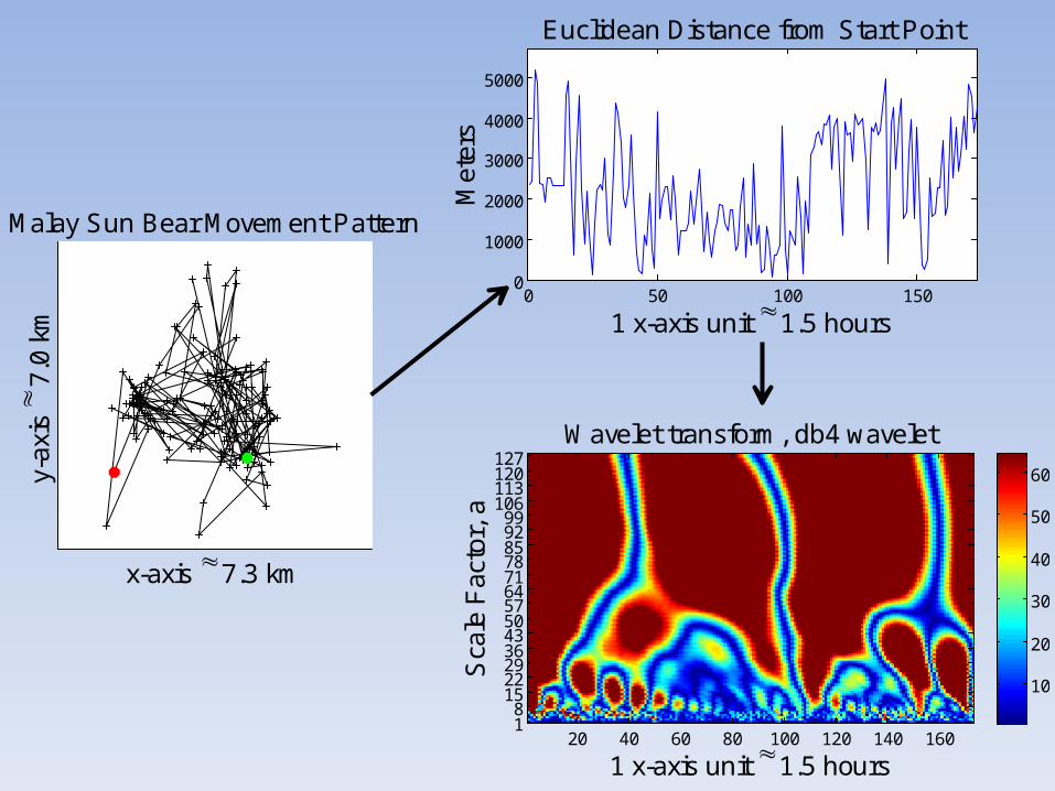
x-axis 7.3 km
y-ax
is
7.0
km
Malay Sun Bear Movement Pattern
0 50 100 1500
1000
2000
3000
4000
5000
1 x-axis unit 1.5 hours
Met
ers
Euclidean Distance from Start Point
Wavelet transform, db4 wavelet
1 x-axis unit 1.5 hours
Sca
le F
acto
r, a
20 40 60 80 100 120 140 160 1 8
15 22 29 36 43 50 57 64 71 78 85 92 99
106113120127
10
20
30
40
50
60
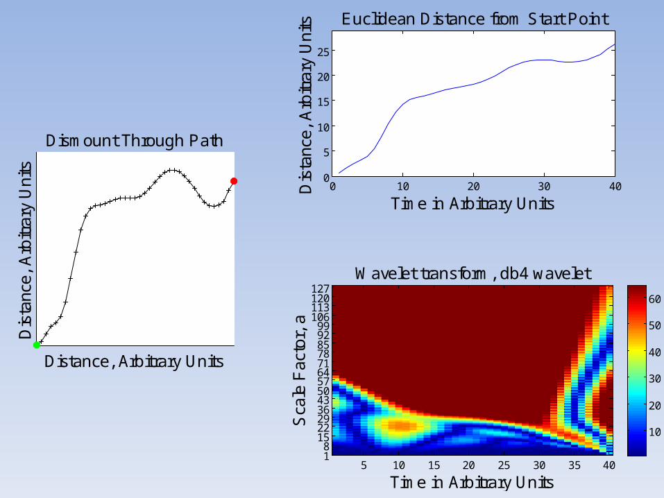
Distance, Arbitrary Units
Dis
tanc
e, A
rbitr
ary
Uni
ts
Dismount Through Path
0 10 20 30 400
5
10
15
20
25
Time in Arbitrary Units
Dis
tanc
e, A
rbitr
ary
Uni
ts Euclidean Distance from Start Point
Wavelet transform, db4 wavelet
Time in Arbitrary Units
Sca
le F
acto
r, a
5 10 15 20 25 30 35 40 1 8
15 22 29 36 43 50 57 64 71 78 85 92 99
106113120127
10
20
30
40
50
60
Analysis of Movement Data
Wavelet Analysis(Discrete) Differential Geometry
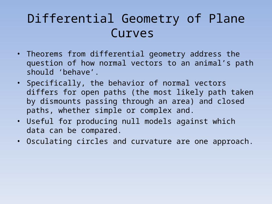
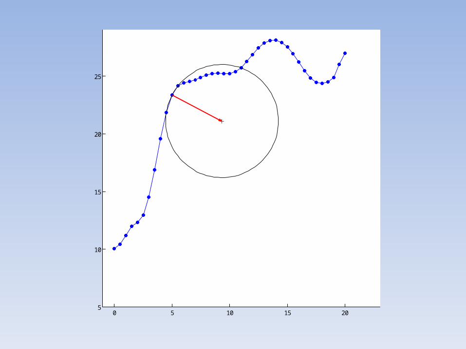
Differential Geometry of Plane Curves
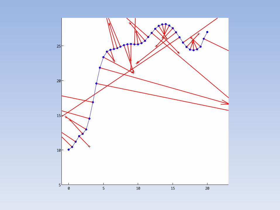
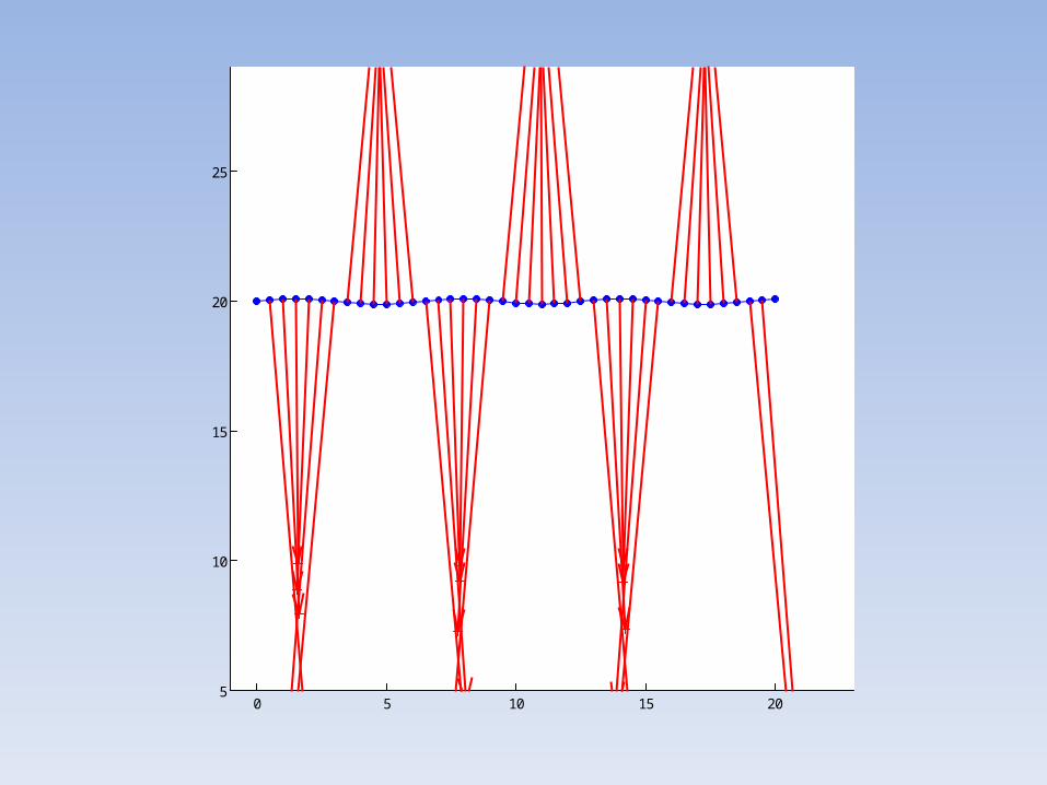
• Theorems from differential geometry address the question of how normal vectors to an animal’s path should ‘behave’.
• Specifically, the behavior of normal vectors differs for open paths (the most likely path taken by dismounts passing through an area) and closed paths, whether simple or complex and.
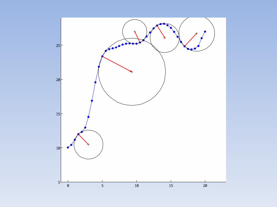
• Useful for producing null models against which data can be compared.• Osculating circles and curvature are one approach.

0 5 10 15 205
10
15
20
25
0 5 10 15 205
10
15
20
25
0 5 10 15 205
10
15
20
25
0 5 10 15 205
10
15
20
25
0 5 10 15 205
10
15
20
25
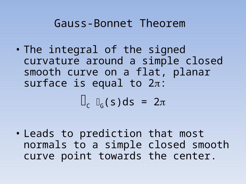
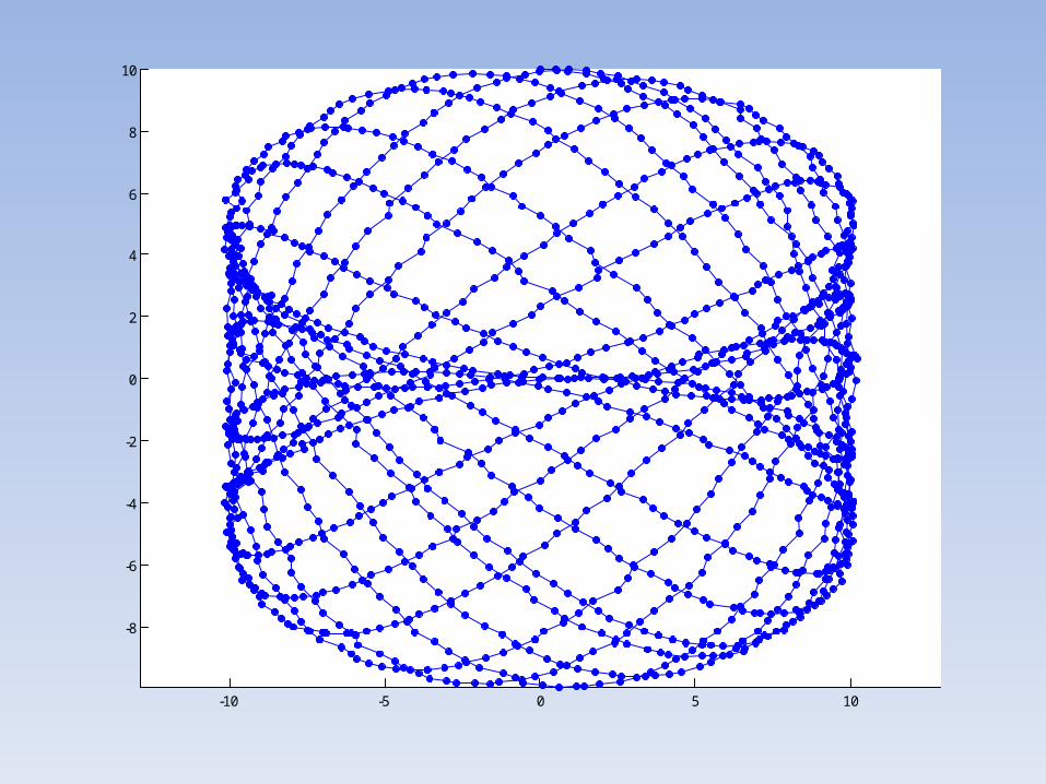
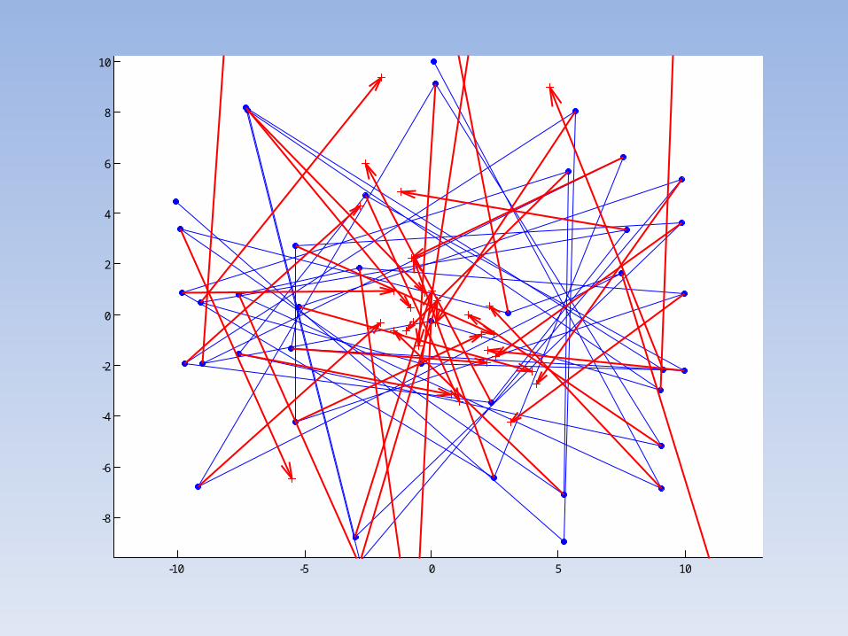
Gauss-Bonnet Theorem
• The integral of the signed curvature around a simple closed smooth curve on a flat, planar surface is equal to 2:
C G(s)ds = 2
• Leads to prediction that most normals to a simple closed smooth curve point towards the center.
-10 -5 0 5 10
-8
-6
-4
-2
0
2
4
6
8
10
-10 -5 0 5 10
-8
-6
-4
-2
0
2
4
6
8
10
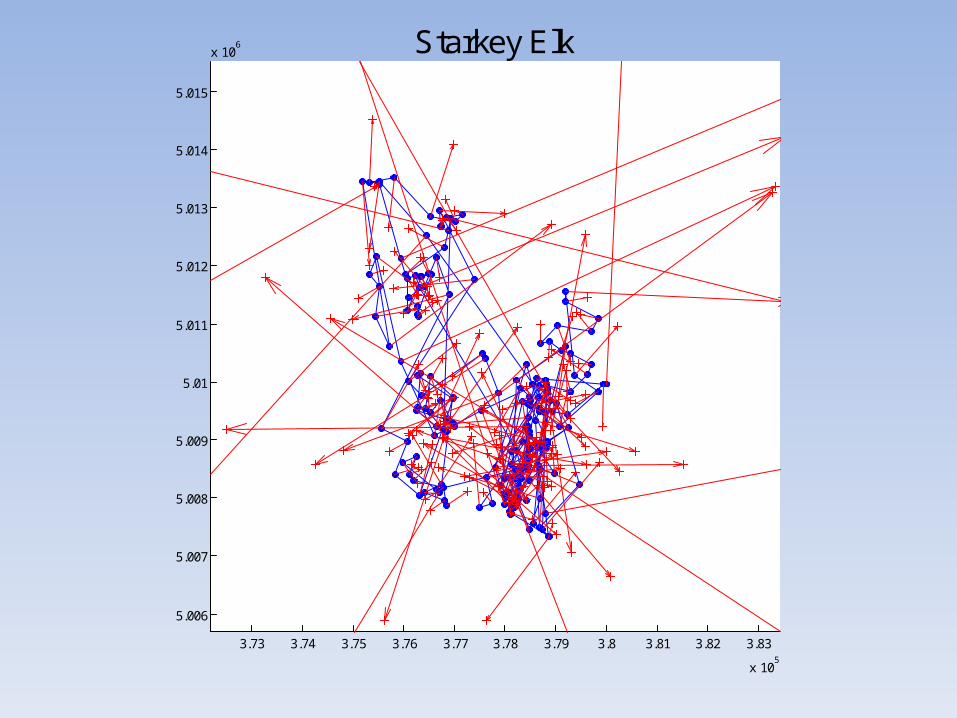
3.73 3.74 3.75 3.76 3.77 3.78 3.79 3.8 3.81 3.82 3.83
x 105
5.006
5.007
5.008
5.009
5.01
5.011
5.012
5.013
5.014
5.015
x 106 Starkey Elk
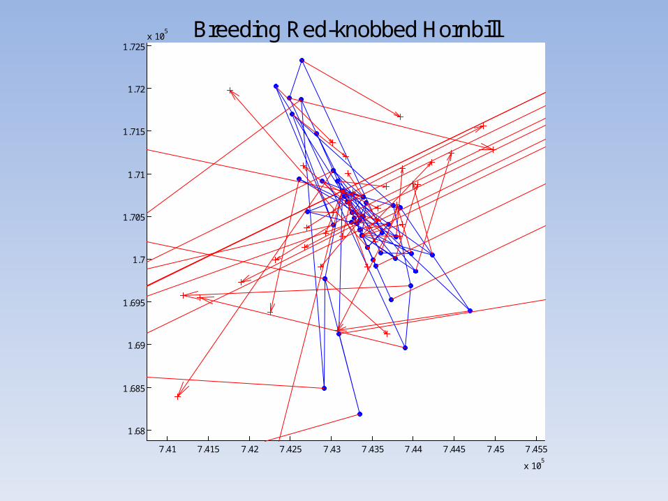
7.41 7.415 7.42 7.425 7.43 7.435 7.44 7.445 7.45 7.455
x 105
1.68
1.685
1.69
1.695
1.7
1.705
1.71
1.715
1.72
1.725x 10
5 Breeding Red-knobbed Hornbill
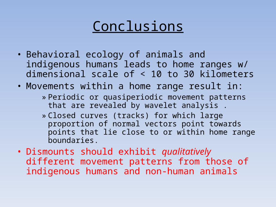
Conclusions
• Behavioral ecology of animals and indigenous humans leads to home ranges w/ dimensional scale of < 10 to 30 kilometers
• Movements within a home range result in:» Periodic or quasiperiodic movement patterns that are
revealed by wavelet analysis .» Closed curves (tracks) for which large proportion of normal
vectors point towards points that lie close to or within home range boundaries.
• Dismounts should exhibit qualitatively different movement patterns from those of indigenous humans and non-human animals

***The following slides would be optional***
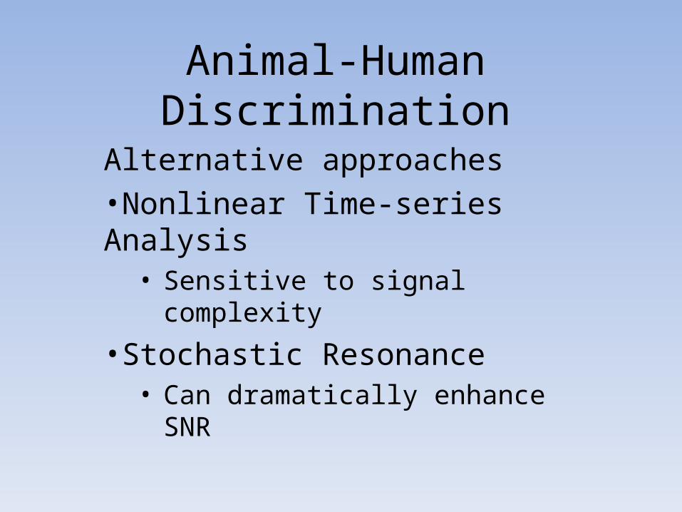
Animal-Human Discrimination
Alternative approaches•Nonlinear Time-series Analysis
• Sensitive to signal complexity
•Stochastic Resonance• Can dramatically enhance SNR
Nonlinear Algorithms
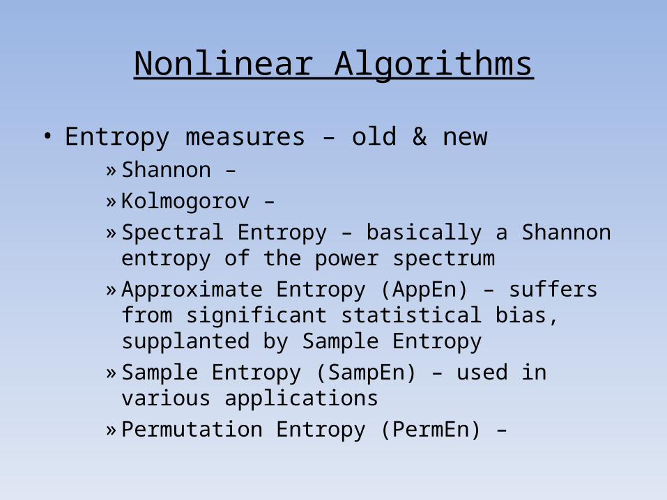
• Entropy measures – old & new» Shannon – » Kolmogorov –» Spectral Entropy – basically a Shannon entropy of the
power spectrum » Approximate Entropy (AppEn) – suffers from significant
statistical bias, supplanted by Sample Entropy» Sample Entropy (SampEn) – used in various
applications » Permutation Entropy (PermEn) –
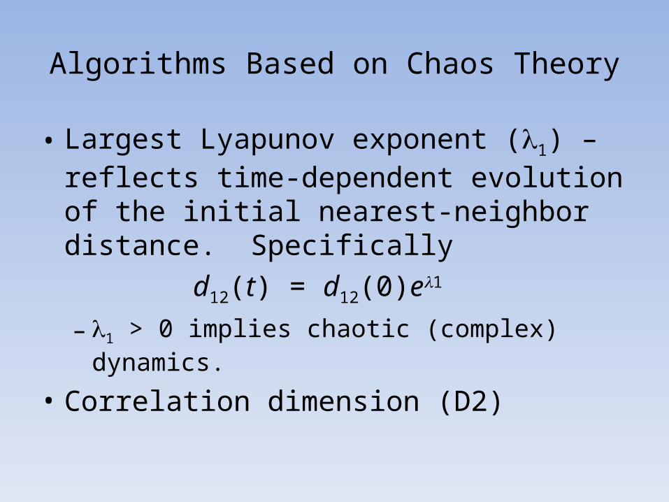
Algorithms Based on Chaos Theory
• Largest Lyapunov exponent (1) – reflects time-dependent evolution of the initial nearest-neighbor distance. Specifically
d12(t) = d12(0)e1 – 1 > 0 implies chaotic (complex) dynamics.
• Correlation dimension (D2)
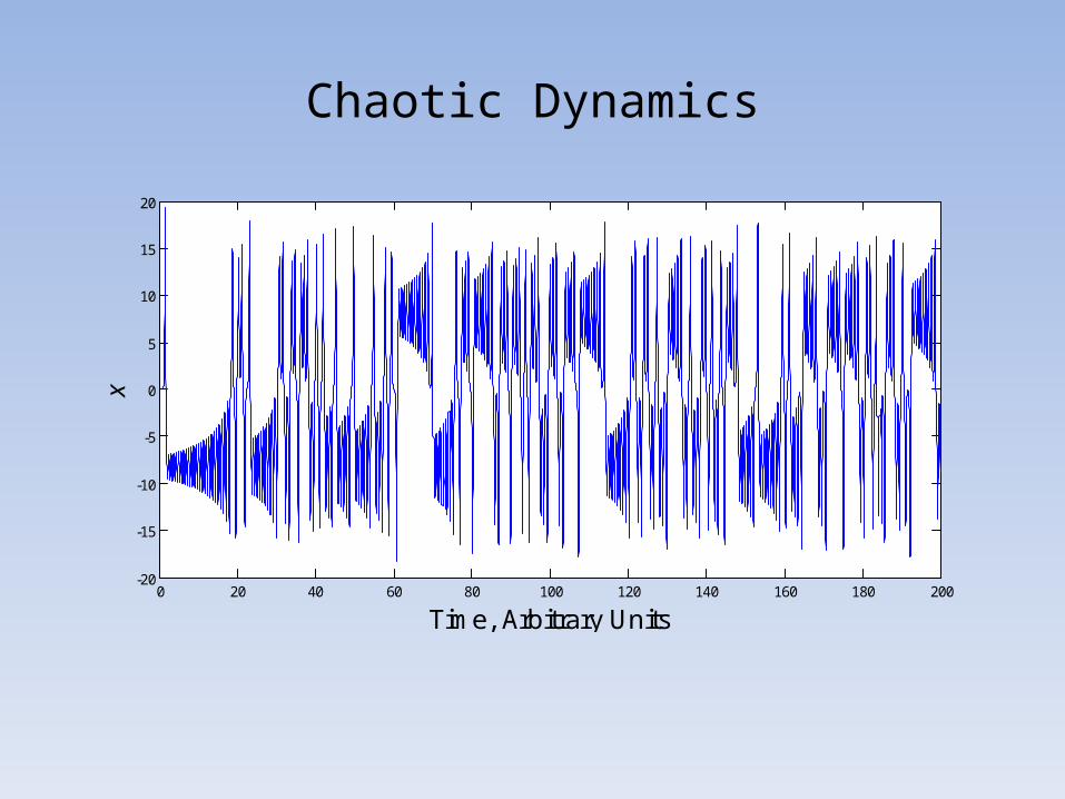
Chaotic Dynamics
0 20 40 60 80 100 120 140 160 180 200-20
-15
-10
-5
0
5
10
15
20
Time, Arbitrary Units
x
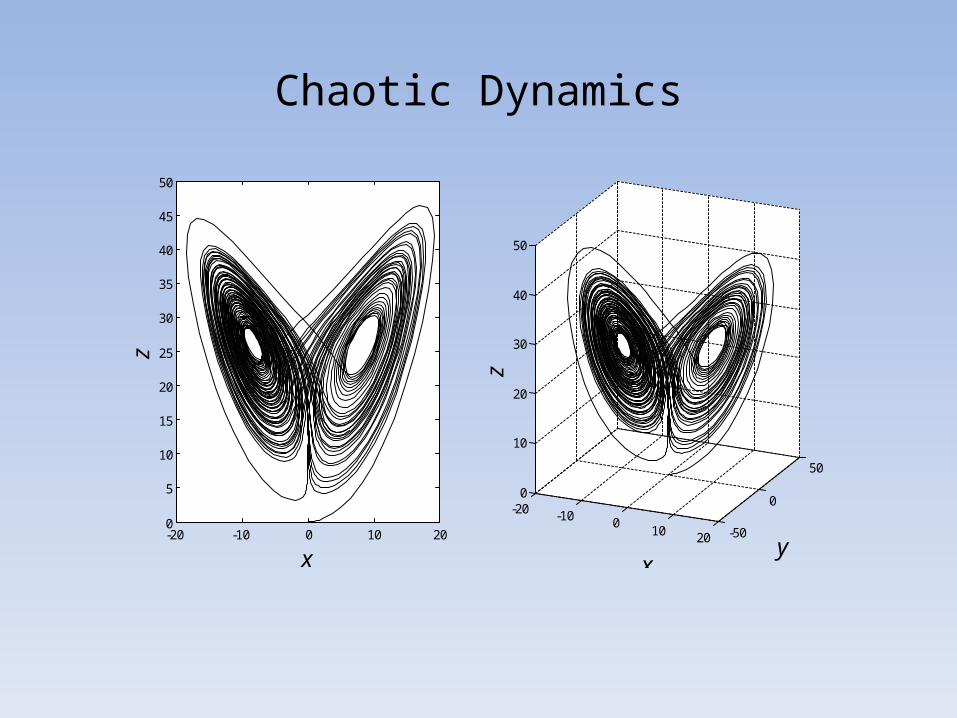
Chaotic Dynamics
-20 -10 0 10 200
5
10
15
20
25
30
35
40
45
50
x
z
-20 -10 010 20 -50
0
50
0
10
20
30
40
50
yx
z
Chaotic Dynamics
0 20 40 60 80 100 120 140 160 180 200-20
-15
-10
-5
0
5
10
15
20
Time, Arbitrary Units
x
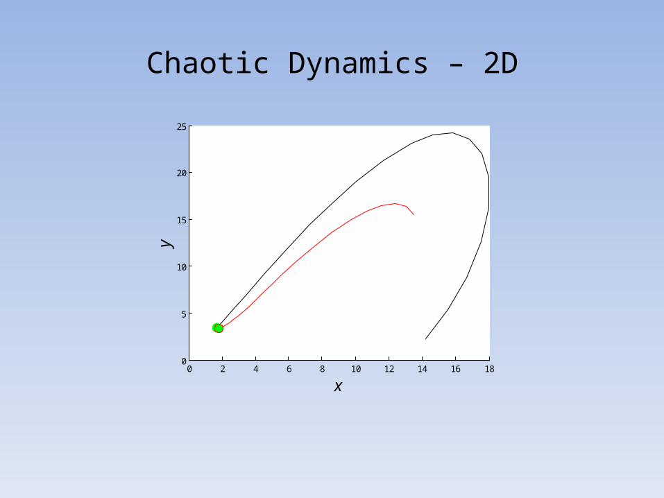
Chaotic Dynamics – 2D
0 2 4 6 8 10 12 14 16 180
5
10
15
20
25
x
y
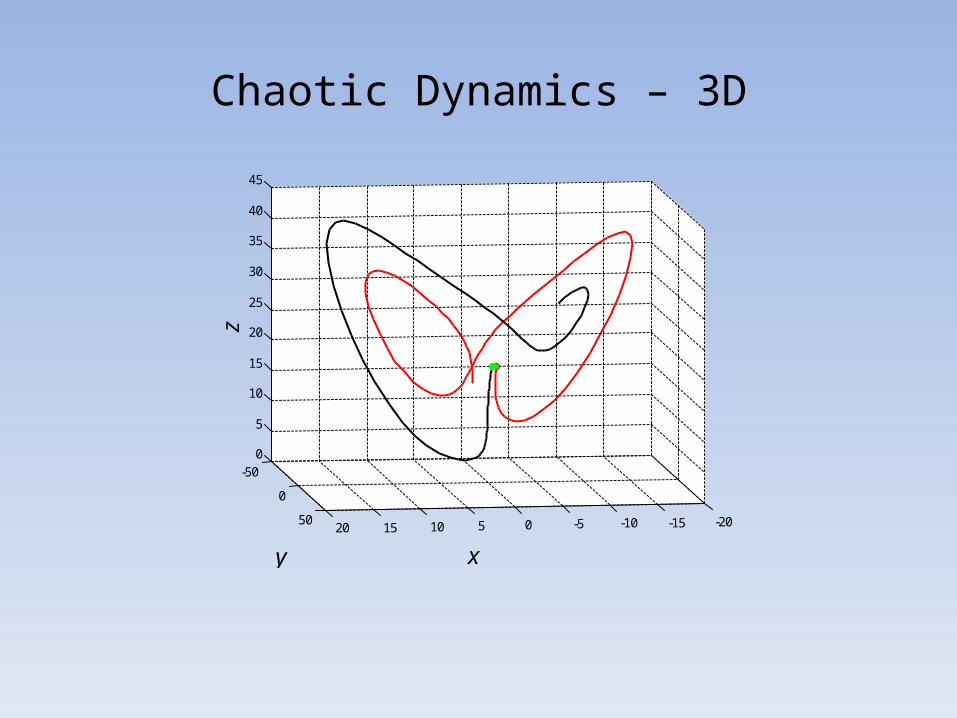
Chaotic Dynamics – 3D
-20-15-10-505101520
-50
0
50
0
5
10
15
20
25
30
35
40
45
xy
z
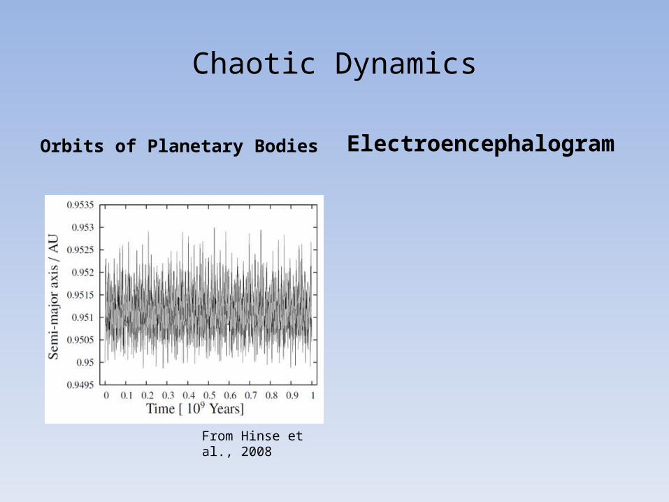
Chaotic Dynamics
Orbits of Planetary Bodies Electroencephalogram
From Hinse et al., 2008
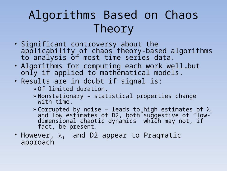
Algorithms Based on Chaos Theory
• Significant controversy about the applicability of chaos theory-based algorithms to analysis of most time series data.
• Algorithms for computing each work well…but only if applied to mathematical models.
• Results are in doubt if signal is:» Of limited duration.» Nonstationary – statistical properties change with time.» Corrupted by noise – leads to high estimates of 1 and low
estimates of D2, both suggestive of “low-dimensional chaotic dynamics” which may not, if fact, be present.
• However, 1 and D2 appear to Pragmatic approach
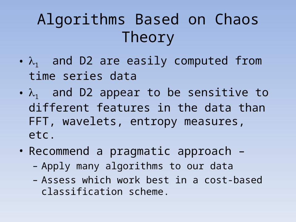
Algorithms Based on Chaos Theory
• 1 and D2 are easily computed from time series data
• 1 and D2 appear to be sensitive to different features in the data than FFT, wavelets, entropy measures, etc.
• Recommend a pragmatic approach – – Apply many algorithms to our data– Assess which work best in a cost-based classification
scheme.
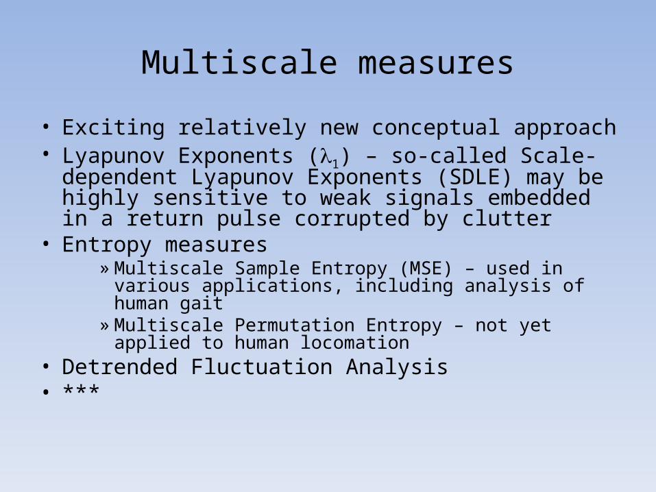
Multiscale measures
• Exciting relatively new conceptual approach• Lyapunov Exponents (1) – so-called Scale-dependent
Lyapunov Exponents (SDLE) may be highly sensitive to weak signals embedded in a return pulse corrupted by clutter
• Entropy measures» Multiscale Sample Entropy (MSE) – used in various
applications, including analysis of human gait » Multiscale Permutation Entropy – not yet applied to human
locomation• Detrended Fluctuation Analysis• ***
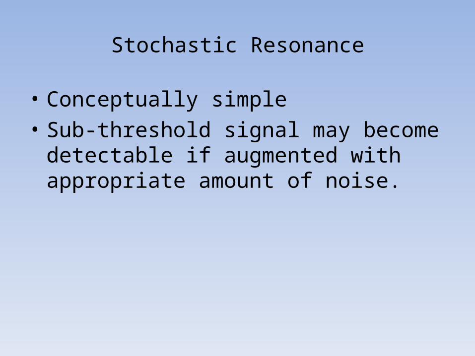
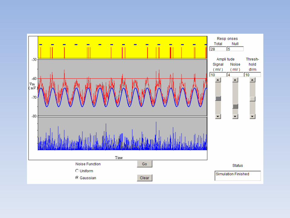
Stochastic Resonance
• Conceptually simple• Sub-threshold signal may become detectable
if augmented with appropriate amount of noise.
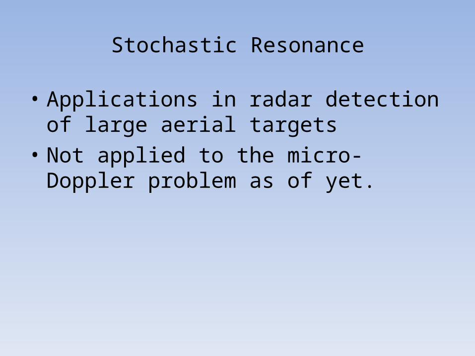
Stochastic Resonance
• Applications in radar detection of large aerial targets
• Not applied to the micro-Doppler problem as of yet.

Have to decide whether to use the following slides and, if so, where to put?
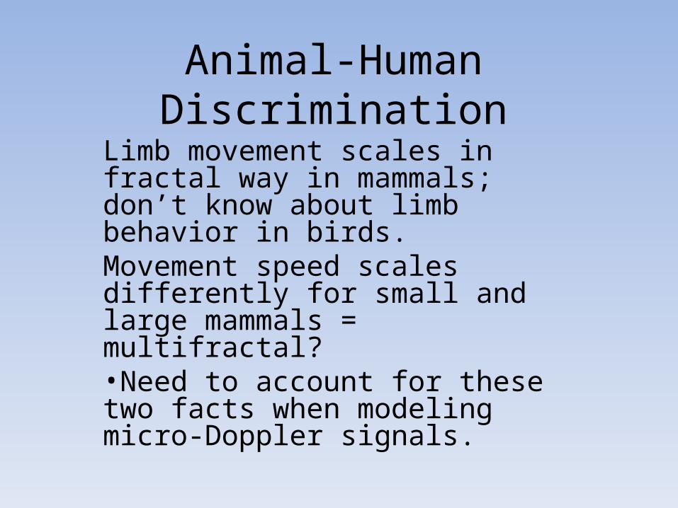
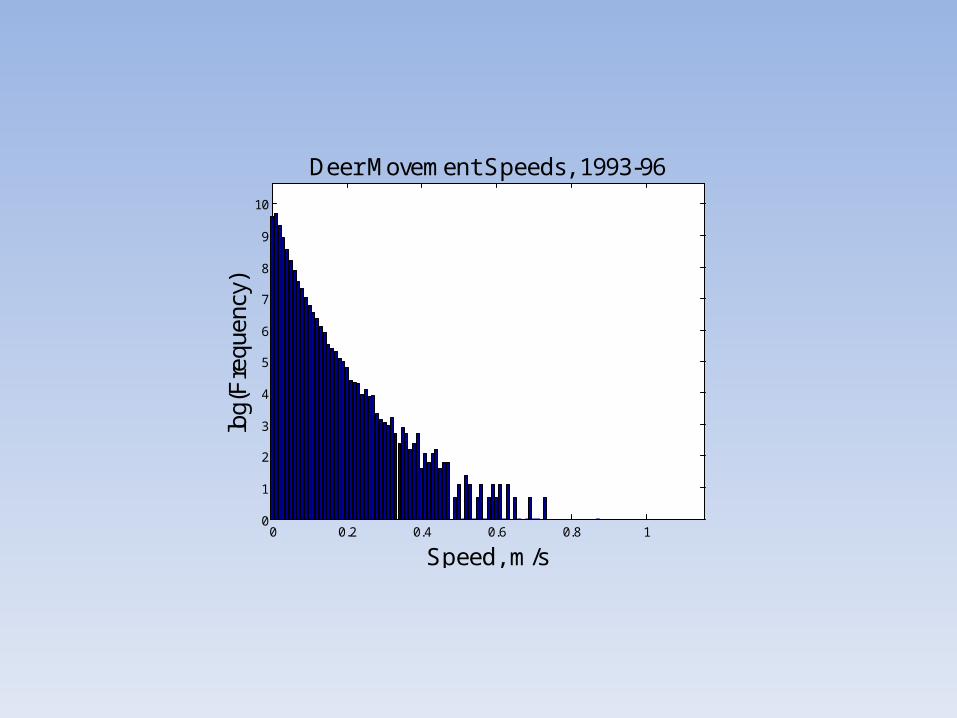
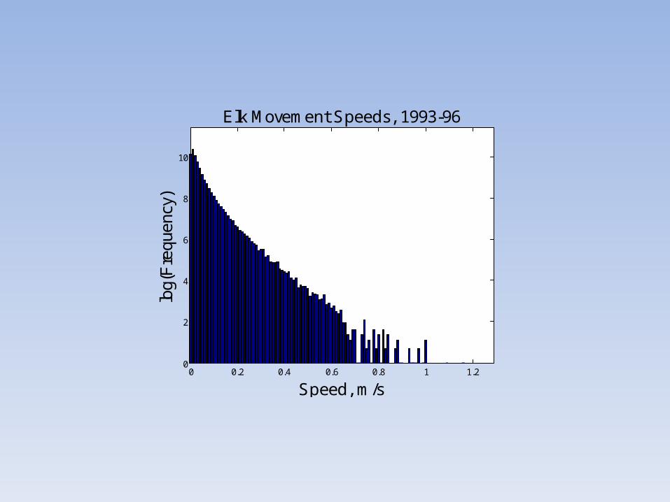
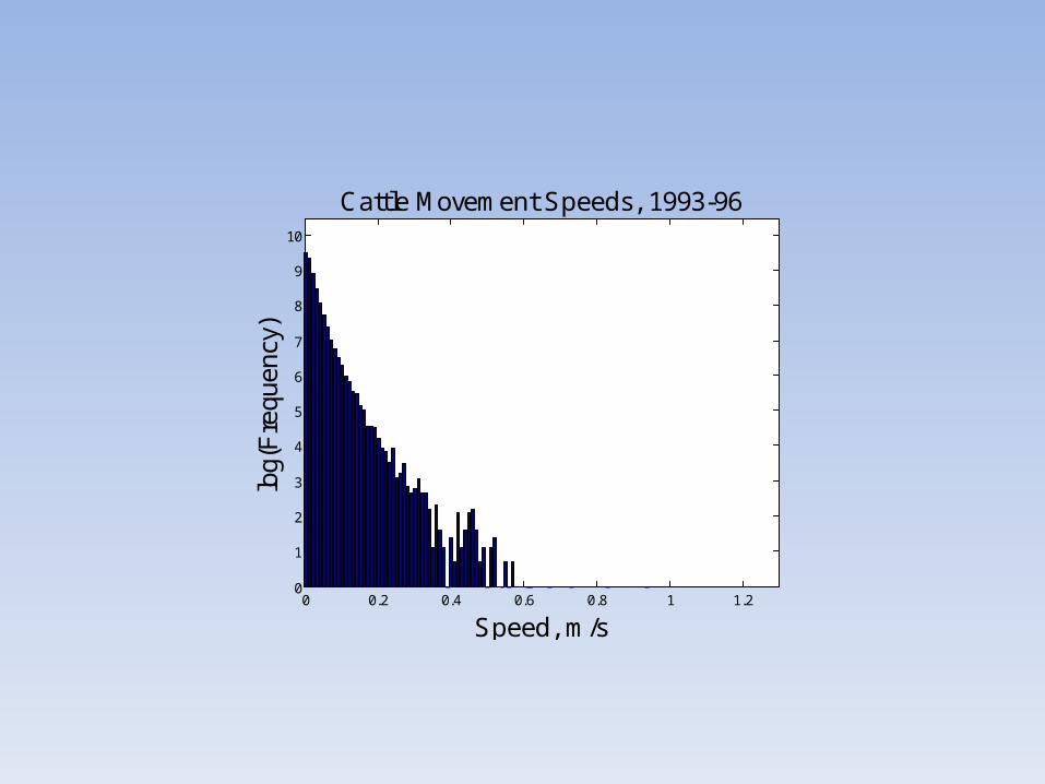
Animal-Human DiscriminationLimb movement scales in fractal way in mammals; don’t know about limb behavior in birds.Movement speed scales differently for small and large mammals = multifractal?•Need to account for these two facts when modeling micro-Doppler signals.
0 0.2 0.4 0.6 0.8 10
1
2
3
4
5
6
7
8
9
10
Deer Movement Speeds, 1993-96
Speed, m/s
log(
Fre
quen
cy)
0 0.2 0.4 0.6 0.8 1 1.20
2
4
6
8
10
Elk Movement Speeds, 1993-96
Speed, m/s
log(
Fre
quen
cy)
0 0.2 0.4 0.6 0.8 1 1.20
1
2
3
4
5
6
7
8
9
10
Cattle Movement Speeds, 1993-96
Speed, m/s
log(
Fre
quen
cy)