effects of emigration on rural labor markets may … · effects of emigration on rural labor...

Effects of Emigration on Rural Labor

Markets

Agha Ali Akram Shyamal Chowdhury Ahmed Mushfiq MobarakYale University

University of Sydney Yale University

May 2017 Preliminary and Incomplete, Do Not Post or Circulate without Authors’ Permission

Abstract Rural to urban migration is integral to scholarship on structural transformation and economic development, but there is little evidence on how out-migration transforms the rural labor market. We offer to subsidize transport costs for 5792 potential seasonal migrants in Bangladesh, randomly varying the proportion of landless agricultural workers across 133 villages induced to move, to generate labor supply shocks of different magnitudes in different villages. We use this variation coupled with a general equilibrium model to document spillover effects on the village labor market. The decision to migrate is a strategic complement: A larger number of simultaneous migration offers in the village increases the likelihood that each individual takes up the offer, and induces those connected to offer recipients to also migrate. The 35% emigration rate in control villages increases to 42% in lower intensity villages, and to 66% with the higher density of offers. This increases the male agricultural wage rate in the village with an elasticity of about 0.2. Migration offers lead to large increases in income earned at the destination, but also increases income earned at home due to the increase in the wage rate and in available work hours. The wage bill for agricultural employers increases, which reduces their profit, with no significant change in yield. There is not much intra-household substitution in labor supply. The primary worker earns more when he returns home from the city during weeks in which many of his village co-residents were induced to move. Although most of the migration income is consumed, there is no systematic effect food prices, suggesting that food markets are better integrated than labor markets across villages. Seasonal migration generates both direct and indirect spillover benefits on the origin economies.

JEL Codes: Keywords: Seasonal migration, spillovers, general equilibrium, Bangladesh. _________________ Contact: [email protected]. We thank Innovations for Poverty Action – Bangladesh team for field and implementation support, Givewell.org for financial support, Mohammad Ashraful Haque, _____ for research assistance, and Sam Asher, Abhijit Banerjee, Ben Faber, Andrew Foster, Edward Glaeser, David Lagakos, Gautam Rao, and conference and seminar participants at Oxford University, Harvard University, Stanford University (IGC/SCID conference), Brown University, DIW-Berlin, BREAD conference, and Yale University for comments.

1

1. Introduction

A shift in labor from rural to urban areas has been integral part of the process of economic

development, and central to theories of long-run growth and structural transformation (Lewis 1954,

Harris and Todaro 1970). Migration marked American agricultural development in the 19th century,

Chinese development in the late 20th century, and has been a feature of the growth path of virtually

every developing country (Taylor and Martin 2001). Understanding the causes and consequences of

mobility – both for the migrant, and for the broader rural society – are therefore central to

understanding development.

A modern literature links migration to development by carefully documenting that workers

are more productive in cities, both within developed (Glaeser and Mare 2001) and developing

(Gollin et al 2001) economies.1 The accompanying empirical literature has largely focused on the

benefits of migration to the migrant and his immediate family (e.g. McKenzie et al 2010, Garlick et

al 2016), but not the spillover effects on the broader rural economy that are surely central to the

links between migration and development. Many scholars have theorized that migration “may

deprive source regions of critically needed human capital,” (Greenwood 1997), “increase rural

poverty and income inequality,” (Connell 1981), but generations of review articles (e.g. Lucas 1997,

Foster and Rosenzweig 2008) lament the lack of evidence on these topics. This study attempts to fill

that gap by conducting a field experiment in which we randomly vary the fraction of landless

households in Bangladeshi villages that are induced to out-migrate temporarily, to generate labor

supply shocks of varying magnitudes, and use those to study spillover effects on the rural economy.

1 This is likely due to the benefits of agglomeration (Combes et al 2010). There is also evidence that cities speed up human capital accumulation, producing growth (and not just level) effects in productivity (Glaeser and Resseger 2010).

2

While social scientists and policymakers have noted the pervasiveness of rural-urban

migration in both developed and developing societies2, the facts that (a) most of this migration is

internal rather than international3, and (b) that much of the internal rural-urban movement is

seasonal and circular in nature, are less well known. The rural-urban wage gap varies within the year

due to crop cycles, and seasonal migration is one of the primary methods used by Indians (Banerjee

and Duflo 2007) and Bangladeshis (Bryan et al 2014) to diversify income and cope with seasonality.

Such seasonal fluctuations in rural labor productivity are widespread in Ethiopia (Dercon and

Krishnan 2000), Thailand (Paxson 1993), Indonesia (Basu and Wong 201x), Malawi (Brune et al

2016) and Ghana (Banerjee et al 2015). Seasonal migration also appears to be more responsive to

policy interventions and to changes in local labor market conditions than permanent migration

(Imbert and Papp 2015).

Bryan et al (2014) encourage a sample of 1292 landless households in rural Bangladesh to

migrate during the 2008 lean season using conditional transfers to cover the roundtrip travel cost to

nearby cities, and show that migration significantly improves the consumption in induced

households. That simple research design can only evaluate the direct effects of migration

opportunities on beneficiary households, and does not answer questions about spillover effects on

non-beneficiaries. We expand on that design in several ways during the 2014 lean season to study

general equilibrium effects on the rural labor market, and in the process, provide a more

comprehensive evaluation of a program to encourage migration.

2 Long (1991) notes that over 6% of the US population migrates internally within a year, and about 20% of the population of US and Canada move over a 5-year interval. Long-run panel data from India and Bangladesh show that 23 percent of men left the village after 17–20 years (Foster and Rosenzweig 2008). 3 There were 240 times as many internal migrants in China in 2001 as there were international migrants (Ping 2003), and 4.3 million people migrated internally in the 5 years leading up to the 1999 Vietnam census compared to only 300,000 international migrants (Ahn et al, 2003).

3

First, in addition to randomly assigning migration subsidies to an expanded sample of 5792

poor landless households, our design also randomly varies the proportion of the eligible population in

the village receiving such offers, because that market-level variation is necessary to track general

equilibrium effects on wages and prices. Second, we collect data from both households that receive

the randomized offers as well as households that do not, to track spillover effects on the migration

and labor supply choices of non-beneficiaries. Third, we collect high-frequency data on earnings and

hours worked by week, by location, and by individual worker, to create a richer description of the

effects of migration including intra-household adjustments in labor supply. Fourth, we collect data

from employers in the village to study effects on market wages, labor costs and profits. Fifth, we

collect price data from local shopkeepers to study equilibrium effects on goods market prices.

We develop a general equilibrium model of the village labor market with endogenous

migration to organize our empirical results on migration, labor supply, earnings, wages and prices.

While the prior literature has explored whether migration generates indirect benefits through risk

sharing (Morten 2015, Munshi and Rosenzweig 2016, Meghir et al. 2016), no study estimates

equilibrium effects on the village economy. Scholars have theorized that migration may increase

rural poverty and income inequality (Connell 1981), or that it has “the effect of draining away from

the rural areas, either temporarily or permanently, some of the strongest, most able, most energetic

young men” (Hance 1970), but empirical evidence on these spillover issues is lacking.4

4 Lipton (1980) counters that the departure of young men would not necessarily lower the productivity or earnings of those left behind. Pritchett (2006) shows using census data that agricultural, coal mining and cotton farming areas of the United States lost 27-37% of its population to emigration between 1930 and 1990, but the population exodus was not accompanied by any large decrease in absolute or relative income. Rempel and Lobdell (1978) informally argue that net remittances are too small to have much effect on enhancing rural productivity, and that remittances are generally consumed not invested. Other scholars (e.g. Ashraf et al 2015) have employed modern research methods to describe remittance behavior and use more rigorously, but have not attempted to tackle effects on the village economy.

4

We find that emigration generates a few different categories of spillovers. First, migration

decisions are strategic complements: a larger number of simultaneous migration subsidy offers in a

village increases each household’s propensity to migrate. Much of the spillover benefit to non-

beneficiaries stem from their own increased propensity to migrate when their neighbors receive

subsidies. Second, although these induced migrants earn much more in nearby cities, the time spent

away does not displace home income. On the contrary, the income that the family earns at home

also increases, due to increases in both the equilibrium agricultural wage rate at home and in

available works hours. We use individual-specific data to explore whether departure of the migrant

induces other household members to supply more labor (Rosenzweig 1988), but find that the

increase in home-income is mostly due to the primary worker earning more when he returns home

from the city during weeks in which many of his village co-residents are away. Third, the increased

agricultural wage rate increases the wage bill for employers and reduces their profit. Fourth, there are

no systematic changes in food prices in the village, which suggests that food markets are spatially

well integrated.

Our results carry several important implications for development theory and policy. First,

the increase in the agricultural wage rate that we document implies that rural labor supply is not as

elastic as labor surplus models (e.g. Lewis 1954) presumed. Second, the marginal product of labor in

agrarian societies is highly seasonal. Models of rural labor markets should be augmented to account

for seasonality, to provide better descriptions of the links between migration and rural development.

Third, our results should encourage policymakers to re-think the various restrictions to internal

mobility they have instituted under the guise of rural development policy (Oberai 1983). Anti-

migration bias remains rampant in policy circles, and many governments, including China,

5

Indonesia, South Africa, have historically reacted to migration as if “it were an invasion to repel”

(Simmons 1981). The large direct benefits for the migrant’s family and indirect benefits for non-

migrants competing in those same labor markets that we document suggest that this mode of

thinking, and the associated restrictions imposed on migrants’ transport, settlement and employment

by policymakers, may be misguided. Concerns about emigration increasing rural poverty and

inequality appear to be unfounded, at least in our context.

This paper also contributes more broadly to the burgeoning economics literature on

program evaluation by developing an experimental and analytical framework that goes beyond

estimation of direct effects on the treated population. Comprehensive evaluation requires

consideration of general-equilibrium changes, especially if we are interested in assessing possible

effects of programs when they are scaled up (Heckman, 1992; Rodrik, 2008; Acemoglu, 2010). For

example, providing skills training to large numbers of beneficiaries (Banerjee et al. 2007; Blattman et

al. 2014) may change skilled wages, or providing livestock assets on a large scale (Banerjee et al 2015,

Bandiera et al 2015) may affect livestock prices. Randomized controlled trials examining aggregate

effects of equilibrium price changes induced by programs implemented on a large scale are still rare5,

but our results suggest that these considerations might be important.

We describe the problem of seasonality and earlier research on seasonal migration in the

next section. We develop a framework to organize our analysis of migration decisions and general

5 One exception is Mobarak and Rosenzweig (2016), who use a general equilibrium model to study labor market effects of rainfall insurance. It is more common for RCTs to track non-market spillovers on the non-treated, including health externalities (Miguel and Kremer 2004), financial transfers (Angelucci and DeGiorgi 2009), and social learning (Kremer and Miguel 2007, Oster and Thornton 2012, Miller and Mobarak 2015). Crepon et al. 2012 and Muralidharan and Sundararaman (2013) study aggregate effects in relevant markets, but do not estimate price or (teacher) wage effects. Cortes (2008) is a non-experimental study exploring the price and wage effects of international migration.

6

equilibrium effects in Section 3. We describe the experiment and the data in Section 4, and present

empirical results in Section 5.

2. Context

2.1 Background on Seasonality and Seasonal Migration

Globally, approximately 805 million people are food insecure (FAO 2016), of which about

600 million are rural residents. Estimated conservatively, half of these people—300 million of the

world’s rural poor—suffer from seasonal hunger (Devereux et al, 2009). In predominantly agrarian

economies, seasonal deprivation often occurs between planting and harvest, while farmers have to

wait for the crop to grow. Labor demand and wages are low during this period, and the prices of

staples like rice tend to increase.

These two facts combine to produce a dire situation in the Rangpur region of Northern

Bangladesh, where rice consumption drops dramatically during the lean season.6 This is an annually

repeating phenomenon known as “monga” in Bangladesh, and by other names in other agrarian

societies around the world (“hungry season” in southern Africa (Beegle et al 2016), and “musim

paceklik” in eastern Indonesia (Basu and Wong 2012)). The landless poor supplying agricultural

labor on others’ farms are especially affected when demand for agricultural labor falls. They

constitute around 56% of the population in our sample area, and will be the target of the seasonal

migration encouragement intervention that we design. Our sampling frame is representative of this

6 Figure A.1 uses nationally representative Household Income and Expenditure Survey (HIES) data collected by the Bangladesh Bureau of Statistics to illustrate these facts. Figure A.2 shows the drop in labor hours and earning capacity in the agricultural sector during the pre-harvest lean season using a different data source (Khandker and Mahmud 2012).

7

landless population in the Rangpur region of Northern Bangladesh. According to the Bangladesh

Bureau of Statistics, there are roughly 15.8 million such inhabitants in Rangpur (BBS, 2011).

According to anthropological accounts, nearby urban and peri-urban areas do not face the

same seasonal downturns, and these locations offer low-skilled employment opportunities during

that same period (Zug, 2006). This contrast suggests a seasonal labor misallocation, or a spatial

mismatch between the location of jobs and the location of people during that particular season.

Inspired by these observations, Bryan et al (2014) conduct a randomized controlled trial to

encourage landless households from the Rangpur region facing seasonal deprivation to migrate

during the Monga period to nearby cities to find work. They document positive effects of migration

on consumption, and then explore why these households were not already migrating. A conditional

transfer of about $8.50-$11 (equivalent to the round-trip travel cost by bus) increases the seasonal

migration rate in 2008 by 22%, increases consumption amongst the migrant’s family members by

757 calories per person per day in 2008 on average, and also induces 9.2% of the treated households

to re-migrate the following year.

Bryan et al (2014) show that the fact that these households were not already migrating in

spite of these large consumption gains can be explained by a model in which people living very close

to the margin of subsistence are unwilling to take on the risk of paying the cost of migration and

sending a member away. Even a small chance that the costly migration fails to generate income

could be catastrophic if the household faces a risk of falling below subsistence. Thus, uninsured risk

creates a poverty trap in which the extreme poor fail to take advantage of migration opportunities

that turn out to be profitable on average. A conditional transfer can address that constraint and

create efficiency gains.

8

2.2 Potential Spillover Effects of Seasonal Migration

Bryan et al (2014) only focused on households that received migration subsidies, not the

spillover effects on non-beneficiaries, or any general equilibrium changes associated with increased

scale of emigration. Consideration of general equilibrium effects requires a fundamentally different,

and more complicated, data collection and experimental strategy that we employ in this study.

To study market-level effects, the scale of our experiment is five times as large, and we

further randomize the proportion of the village population induced to migrate. This design, coupled

with data on both households that receive these offers and households that do not, and data from

employers and grocers, allow us to report results on general equilibrium effects in labor and food

markets. This has become a policy-relevant question, because implementers and funding agencies

are advocating for and deploying seasonal migration subsidies in large scale as a social policy to

counter seasonal poverty (Evidence Action 2016). Such scale up should be evaluated in terms of

both direct and indirect effects.

3. Experiment and Data

The next two sub-sections set out the details of the experiment and the data collection.

Figures 1 and 2 provide a visual account of the main features of the experiment and the type and

timing of data collection.

3.1 Intervention

The basic form of our intervention was the offer of a cash grant worth Taka 1,000 ($13.00

USD) to rural households in northern Bangladesh to cover the round-trip cost of travel to nearby

cities where there are job opportunities during the lean season. This is a conditional transfer, where

9

the subsidy is conditional on one person from the household agreeing to out-migrate during the lean

season. As offers were made, we let households know that they may have a better chance of finding

work outside of their village, but we did not offer to make any connections to employers. No

requirement is imposed on who within the household has to migrate, or what city they have to go to.

As in Bryan et al (2014), migration was carefully and strictly monitored by project staff to ensure

adherence to the conditionality.

3.1.1 Sampling

The experiment was conducted in 133 randomly selected villages in Kurigram and

Lalmonirhat districts of Rangpur. We first conducted village censuses to identify all households that

would be “eligible” to receive this intervention in each of these villages. A household was deemed

eligible if (1) it owns less than 0.5 acres of land, and (2) it reported back in 2008 that a member had

experienced hunger (i.e., skipped meals) during the 2007 monga season. We focused on

landownership because land is the most important component of wealth in rural Bangladesh, and it

is easily measurable and verifiable. We used the second question on skipping meals to avoid

professional, non-agricultural households (who may not own much land, but who are comparatively

well off). Our census data suggests that about 57% of households in these villages were eligible to

receive the intervention after applying these two criteria.

3.1.2 Random Assignment

We randomly assigned the 133 villages into three groups:

(a) Low Intensity – 48 villages where we targeted migration subsidies to roughly 14% of the

eligible population.

10

(b) High Intensity – 47 villages where we targeted roughly 70% of the eligible population with

migration subsidy offers.

(c) Control – 38 randomly selected villages where nobody is offered a migration subsidy.

The high vs low intensity design was chosen to generate significant variation in the size of

the emigration shock, but the precise target (14% vs 70%) varied a little across villages within

treatment arms. This is because our village population estimates were dated (from 2008) for most

(100) villages, and imprecise in the 33 other villages, which made it difficult for us to precisely

estimate the ratio (offers/eligible population) in each village.

The sample of 133 villages included the 100 villages that were part of the earlier Bryan et al

(2014) experiment, but the majority of the households in our sample are new, and were not included

in the earlier experiment. We show in Appendix Tables A2-A4 that participation in the earlier

rounds of the experiment has no significant effect on migration decisions this year, and therefore

does not materially affect the main results of this paper on the downstream effects of migration on

income earned. Controlling for village level random assignment in the earlier rounds does not affect

our results either.

Landless households are engaged in both agricultural and non-agricultural work. We had

provided experimental instructions to target non-agricultural households first in some (randomly

chosen) villages, and our randomization of low vs high intensity was stratified and perfectly balanced

by this instruction. During implementation we learned that in reality most households supply labor

to some form of agriculture. We show in Tables A2-A4 that the stratification had no effect on

migration decisions, nor does it affect our estimates of the effect of treatment intensity on migration

or income outcomes.

11

There were a total of 883 subsidy offers made in the 48 low-intensity villages, 4,881 subsidy

offers made in the 47 high intensity villages. The total number of households resident in these 133

villages was 36,808.

3.1.3 Timing

We disbursed grants during the latter part of the monga season, in early November, 2014.

Figure 2 provides a timeline of project activities. Ideally, seasonal migration subsidy offers should

be made in September after the rice planting work is done, but our disbursement was delayed due to

political disturbance in Bangladesh at that time. Despite this delay, we observe high overall take-up

and migration during both the late Monga, and as well as some post-harvest migration after January.

We will also report results on re-migration a year later, covering the full 2015-16 migration season.

3.1.4 Implementing Organizations

All of the implementation activities – the offers and marketing, grant disbursement, and

monitoring to ensure adherence to the conditionality, were conducted by RDRS, a local NGO with

a long history of engagement in Rangpur, and substantial presence in the region. RDRS runs a

microfinance program among other poverty alleviation activities, and this expertise was useful to

handle the disbursement of grants, and ensure recovery of funds in cases of non-compliance with

the condition associated this grant.

Innovations for Poverty Action in Bangladesh (IPA-B) coordinated all research activities and

was responsible for testing and fielding surveys, collecting, cleaning and maintaining data. They also

monitored RDRS’ implementation activities to ensure that they were conducted in accordance with

the research protocol.

3.1.5 Protocol and Logistics

12

After the research team conducted the sampling and randomization, they provided RDRS

staff a list of eligible households in the village and their treatment assignment, and RDRS staff are

deployed to the village to implement the intervention. Staff members approach a specific household

on their list and first verify that they satisfy the eligibility criteria. Then the household is offered the

grant to migrate, and the conditionality is made explicit. The head of the household is told that it if it

accepts the grant, one member must use it toward migration travel expenses, and that this will be

monitored. Households were also informed that nearby areas may offer better chances of

employment than their home village.

Once the conditions of the offer are explained clearly, the household is provided guidance

on how to collect the grant funds from their local RDRS office. The staff member collects

identification information from the household. If the beneficiary visited the RDRS office to collect

the grant, an officer checked their ID before disbursing funds. The grant amount (1000 Taka) was

large enough to cover the cost of a round trip bus ticket to nearby popular urban destinations, with

some money left over for a few days of board and lodging.7

RDRS carefully monitored adherence to the conditionality. After funds disbursement, an

RDRS officer visited the household to check whether someone had migrated or not. If no one had

migrated at the time, the officer reminded the head of household that the grant he received was

conditional on migration and if he would not migrate he would be required to return the funds. The

officer made two more visits to the households that had failed to migrate, and requested that funds

be returned in migration still had not taken place.

7 We considered the possibility of providing bus tickets to migrants, but the logistics of contracting with multiple transport companies, and finding flexible means to match transporters to migrants were too daunting. Previous experience also suggested that it was possible to get beneficiaries to adhere to the migration condition, so we settled on cash transfers.

13

3.2 Data Collection

We conducted four separate types of surveys in 2014-15 to capture effects on the labor

market choices, other household impacts, effects on employers, and effects on food prices. We

conducted two additional surveys a year later (after the lean season in the following year) to capture

longer-term persistent effects on households and employers in 2015-16. Figure 1 depicts sample

sizes by experimental cell, Figure 2 lays out the timeline of data collection and intervention activities

relative to the agricultural season.

3.2.1 High Frequency Labor Market Survey of Households

Soon after the travel grants were disbursed in November 2014, we started surveying 2294

households in both treatment and control villages about their wage and employment conditions. The

survey was administered once every 10 days for six rounds starting on December 22, 2014. We

therefore refer to this as the “High Frequency Origin Survey”. The survey instrument asked

respondents about labor market outcomes (income, time spent working, location, industry) and a

brief set of questions on consumption (essential food and non-food items) and migrant remittances.

We focus on income and labor market outcomes given our interest in general equilibrium

effects, in contrast to Bryan et al (2014), who largely focused on consumption to evaluate the direct

effects of inducing migration. Income is generally thought to be more difficult to measure well in

rural, agrarian areas of low income countries due to seasonal variation, multiplicity in sources of

income, weekly variation in activities over the course of the agricultural cycle, self-employment and

family employment (Deaton and Muellbauer 1982). This is why we engage in a very expensive

method of surveying, visiting households six times on an almost weekly basis and asking about

income-generation activities of all household members over only the previous week to minimize

14

recall bias. We also conduct the surveys during a narrow two-month window during which seasonal

and employment variation is minimized. The surveys focus on landless households that have

minimal self-employment or unpaid family employment on their own farm. This provides us with

labor supply choices of all working individuals within each household, the location where they

worked (inside the village or at migration destinations), and how much they earn on a daily basis.

This method of surveying produces some ancillary benefits. First, it allows us to track high-

frequency movements back and forth between the village and the city. Many migrants travel for only

3-4 weeks at a time and engage in multiple trips during the season. We observe 1.6 trips per migrant

on average in our data. Second, the technique also allows us to track intra-household substitutions in

labor supply, because we collect data at the individual level. Third, it allows us to cross-validate the

direct (income) effects of migration that we estimate, with the consumption outcomes Bryan et al

(2014) collected using a completely different surveying method six years prior, but administered on a

similar population chosen using the same sampling frame. The magnitudes of income and

consumption effects need to be coherent. Fourth, we can also validate our income estimates from

the high-frequency survey using income measures collected at the endline household survey we

ourselves conduct a few months later. The endline survey, conducted on an overlapping sample of

households, asked about migration experience and income during the same season, described in

further detail below.

The high-frequency surveys were administered to 709 households that did not receive

migration offers in treatment villages, in addition to 865 households that did. Our goal was to track

whether offers to a certain sub-group of households lead others to migrate, and track any spillover

income and employment effects on those households either at home or at the destination.

15

3.2.2 Food Price Data: High Frequency Survey of Shopkeepers

We pair the brief consumption module in the high-frequency survey described above with a

survey of shopkeepers (i.e. grocery store owners) that was administered simultaneously, in order to

collect prices for the same food items that the consumption module asked households about. We

collected data on the prices of major food items, including rice, wheat, pulses, edible oil, meat, fish,

eggs, milk, salt and sugar. These data allow us to explore whether encouraging migration at large

scale in a village (and the extra income that generates) leads to a general equilibrium effects on food

markets. It also allows us to convert the food consumption effects to monetary values.

3.2.3 Endline Survey

Next, we conducted a detailed endline survey of 3,602 households during April 2015, before

the next rice planting season starts. Figure 1 displays the sample breakdown across treatment arms

and across types of households (those offered grants and those who were not). This endline survey

collected a broader set of information on migration and other socio-economic outcomes that were

not sensible or possible to ask repeatedly on a weekly basis, as in the high frequency survey. Core

modules focused on collecting detailed information on the migration experience, including number

of members who migrated, timing of migration events and destinations. The survey also delved into

income generated by households (especially from migration), behavior and attitude changes, risk

coping, credit and savings.

3.2.4 Employer Survey

To measure impacts on the demand-side of the labor market we conducted a survey of 1,099

employers across all villages on the wages they paid for employees around (and after) the time that

we disbursed migration grants. We also asked employers to provide qualitative assessments of the

16

ease of finding and hiring workers during that period. We collected data on wages for multiple

activities in both agricultural and non-agricultural sectors, separately for males and females hired

(since almost all seasonal migrants are male). Unlike the high-frequency wage survey, the employer

survey was retrospective, and asked employers to recall wage and employment conditions for every

two-week period starting mid-October through the end of December 2014. We are confident of

high quality recall because (a) our survey referred to wages paid for specific agricultural activities (e.g.

for planting or for harvest), (b) employers tend to maintain records for their businesses, and (c)

survey staff were trained to prompt employers with cues on types and timing of events (e.g.

associating the timing of a given employment activity with a significant cultural or religious event).

3.2.5 Follow-up Survey 2016: Households

To study the longer-term behavior of households, we conducted a follow-up survey in 2016

enquiring about a number of items over the time period beginning mid-August 2015 through mid-

August 2016. This survey included questions on migration – specifically, timing and number of

episodes, income from migration and questions about resource-sharing by migrants – and the

household’s experience of hunger over the previous year. This was administered to the original

endline sample from the 2014-2015 round of study and we were able to effectively re-interview

3,386 households (from the original 3,602).

3.2.6 Follow-up Survey 2016: Employers

The second component of our follow-up survey work targeted the demand-side of the labor

market i.e. employers. We administered a labor demand and wage survey to agricultural employers to

better understand the impacts of emigration on their enterprise and decisions. The employer labor

demand and wage survey was administered to 649 employers across all 133 villages.

17

4. Theory

4.1 Offer Intensity and Migration

Our theory characterizes the response of rural labor markets to labor supply shocks

(migration). We define a village as the local labor market in which two types of households interact:

a. Landless households that supply labor

b. Landed farmers that hire labor

Our intervention targeted landless households. In any given village, a proportion, , of

landless households was provided a travel grant, . The proportion that received the grant was

experimentally varied. A member of a landless household that receives the grant, , decides to

migrate if the value of migration is greater than wage income from the local labor market,

(4.1.1)

Where, is wage at migration destination, is the migration subsidy conditional on

migration, is the individual specific cost of migration, is the cost of migration that can be

shared with other migrants (hence a function of ) and is the village wage. can be interpreted

as sharing risk as well, and both and can be influenced by .

And for the remaining 1 households (those who did not receive the grant) decide to

migrate if,

(4.1.2)

In the above, we assume that the individual cost of migration is distributed,

~ . (4.1.3)

18

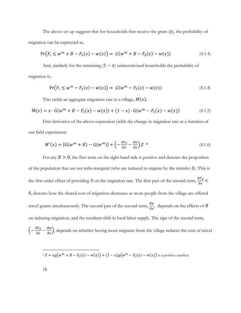
The above set up suggests that for households that receive the grant ( ), the probability of

migration can be expressed as,

Pr (4.1.4)

And, similarly for the remaining (1 ) unincentivized households the probability of

migration is,

Pr (4.1.4)

This yields an aggregate migration rate in a village, ,

M ∙ G 1 ∙ G (4.1.5)

First derivative of the above expression yields the change in migration rate as a function of

our field experiment:

G G 8 (4.1.6)

For any 0, the first term on the right-hand side is positive and denotes the proportion

of the population that are not infra-marginal (who are induced to migrate by the transfer B). This is

the first order effect of providing B on the migration rate. The first part of the second term,

0, denotes how the shared cost of migration decreases as more people from the village are offered

travel grants simultaneously. The second part of the second term, , depends on the effects of

on inducing migration, and the resultant shift in local labor supply. The sign of the second term,

, depends on whether having more migrants from the village reduces the cost of travel

8 1 is a positive number.

19

(by permitting sharing) by more than the benefits of staying back at home to take advantage of the

fact that wages will not fall by as much when many other people in the village emigrate. The relative

size of these two factors is testable in our setting: We can compare how each individual receiving a

migration subsidy (B) in the low- versus high- intensity village respond to the offer. The response to

the exact same offer of B will be stronger in the high intensity village if is larger in

magnitude than .

4.2 Income and Wage in Origin Labor Market

Suppose each landless household who has not migrated out has a Cobb-Douglas utility

function,

(4.2.1)

Where denotes consumption goods measured in taka and are hours of leisure. is

given by,

Where is labor hours supplied within the village, is wage in the village, is outside

income including income from migration. The time constraint function is given by,

1

The household maximizes expected utility subject to the budget and time constraint,

Max 1 (4.2.2)

The FOC condition is,

Control

Villages: 38Offers: 0

Low Intensity

Villages: 48Offers: 883

High Intensity

Villages: 47Offers: 4,881

• Hi-Freq Survey: 722• Endline Survey:

• 697• 655


• 814• 760


• 975• 910


• 558• 520


• 562• 541

• Grocer Survey: 114 • Employer Survey:

• 316• 182

• Grocer Survey: 144• Employer Survey:

• 401• 237

• Grocer Survey: 141• Employer Survey:

• 382• 230

Fig 1: Experimental Design to understand GE

Offered Household

Non-offered Household

Endline survey and the employer survey administered twice.

Fig 2: Intervention and Data Collection Calendar

Sep Oct Nov Dec

Endline Survey

Grant Handout

2014 2015

Employer SurveyHigh FrequencyOrigin Survey

High Frequency Origin Survey

1 2 3 4 5 6

6 survey rounds in 8 weeks to ask about labor hours and wage income by location, minimizing recall bias.

Monga2014

Mini‐Monga2015

Monga2015

Mini‐Monga2016

Jan Feb Mar Apr May Sep Oct Nov DecJun … Aug Jan Feb Mar Apr May Jun Jul Aug Sep

• Endline Re‐survey• Employer Re‐survey

2016

(1) (2) (3) (4)

VARIABLESAt least one migrant

(2014-15)

Number of migrants

(2014-15)

Migration episodes

(2014-15)

Re-migration in 2016

at least one migrant

0.248*** 0.260*** 0.390*** 0.188***

(0.0366) (0.0409) (0.0669) (0.0341)

0.0333 0.0318 0.0660 0.0282

(0.0388) (0.0442) (0.0730) (0.0347)

0.398*** 0.415*** 0.618*** 0.293***

(0.0333) (0.0382) (0.0636) (0.0352)

0.0965** 0.111** 0.123* 0.127***

(0.0397) (0.0463) (0.0742) (0.0371)

Mean in control 0.34 0.37 0.50 0.38

Observations 3,600 3,600 3,600 3,382

R-squared 0.14 0.12 0.12 0.09

Upazila FE YES YES YES YES

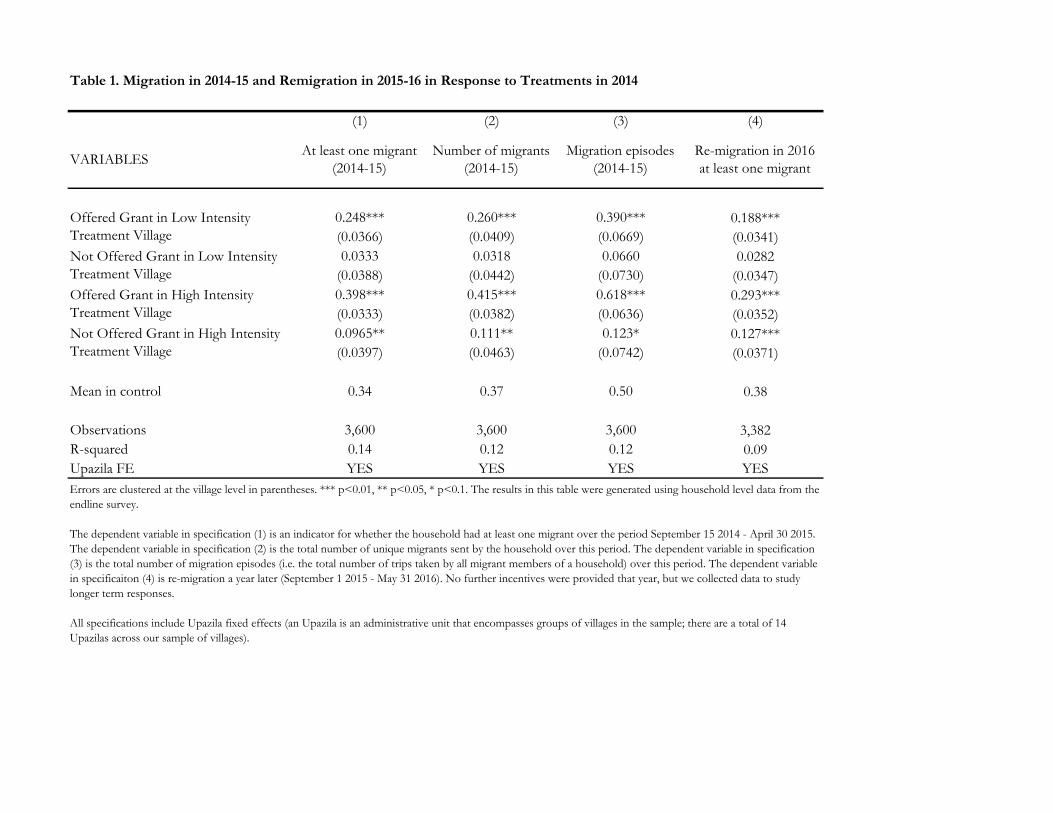
Errors are clustered at the village level in parentheses. *** p<0.01, ** p<0.05, * p<0.1. The results in this table were generated using household level data from the

endline survey.

The dependent variable in specification (1) is an indicator for whether the household had at least one migrant over the period September 15 2014 - April 30 2015.

The dependent variable in specification (2) is the total number of unique migrants sent by the household over this period. The dependent variable in specification

(3) is the total number of migration episodes (i.e. the total number of trips taken by all migrant members of a household) over this period. The dependent variable

in specificaiton (4) is re-migration a year later (September 1 2015 - May 31 2016). No further incentives were provided that year, but we collected data to study

longer term responses.

All specifications include Upazila fixed effects (an Upazila is an administrative unit that encompasses groups of villages in the sample; there are a total of 14

Upazilas across our sample of villages).

Table 1. Migration in 2014-15 and Remigration in 2015-16 in Response to Treatments in 2014

Offered Grant in Low Intensity

Treatment Village

Not Offered Grant in Low Intensity

Treatment Village

Offered Grant in High Intensity

Treatment Village

Not Offered Grant in High Intensity

Treatment Village

(1) (2)

VARIABLESAt least one migrant

(2014-15)

At least one migrant

(2014-15)

0.209*** 0.191***

-0.0444 -0.0526

0.226***

(0.0522)

0.208*** 0.216***

-0.0637 -0.0636

0.0991* 0.122*

-0.0556 -0.0678

0.0666

(0.0772)

-0.0443 -0.0473

-0.137 -0.137

0.311*** 0.344***

-0.0589 -0.0717

0.249***

-0.0692

0.112

-0.374

0.126** 0.156*

(0.0632) (0.0833)

0.0686

(0.0865)

-0.213 -0.173

(0.23) (0.245)

Mean in control 0.33 0.33

Observations 998 994

Upazila FE YES YES

Table 2. Effect of Household's Network on Probability of Migrating in 2014-15

Not Offered Grant in High Intensity Treatment Village and

Connected to Someone Offered

Not Offered Grant in High Intensity Treatment Village and

Partially Connected to Someone Offered

Not Offered Grant in High Intensity Treatment Village and Not


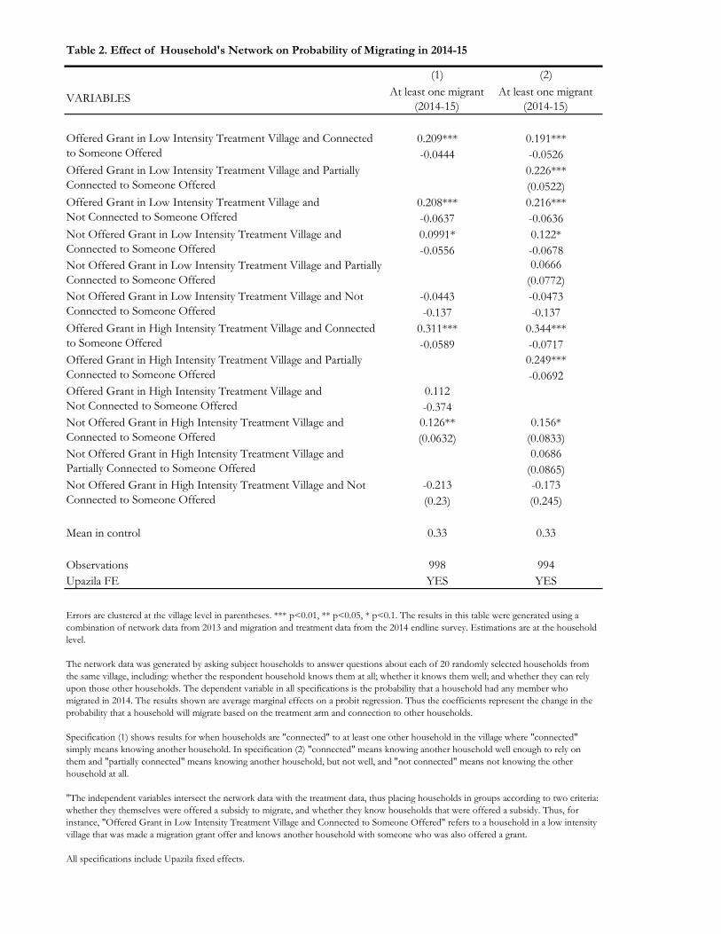
Errors are clustered at the village level in parentheses. *** p<0.01, ** p<0.05, * p<0.1. The results in this table were generated using a

combination of network data from 2013 and migration and treatment data from the 2014 endline survey. Estimations are at the household

level.

The network data was generated by asking subject households to answer questions about each of 20 randomly selected households from

the same village, including: whether the respondent household knows them at all; whether it knows them well; and whether they can rely

upon those other households. The dependent variable in all specifications is the probability that a household had any member who

migrated in 2014. The results shown are average marginal effects on a probit regression. Thus the coefficients represent the change in the

probability that a household will migrate based on the treatment arm and connection to other households.

Specification (1) shows results for when households are "connected" to at least one other household in the village where "connected"

simply means knowing another household. In specification (2) "connected" means knowing another household well enough to rely on

them and "partially connected" means knowing another household, but not well, and "not connected" means not knowing the other

household at all.

"The independent variables intersect the network data with the treatment data, thus placing households in groups according to two criteria:

whether they themselves were offered a subsidy to migrate, and whether they know households that were offered a subsidy. Thus, for

instance, "Offered Grant in Low Intensity Treatment Village and Connected to Someone Offered" refers to a household in a low intensity

village that was made a migration grant offer and knows another household with someone who was also offered a grant.

All specifications include Upazila fixed effects.

Offered Grant in Low Intensity Treatment Village and Connected

to Someone Offered

Offered Grant in Low Intensity Treatment Village and Partially


Offered Grant in Low Intensity Treatment Village and

Not Connected to Someone Offered

Not Offered Grant in Low Intensity Treatment Village and


Not Offered Grant in Low Intensity Treatment Village and Partially


Not Offered Grant in Low Intensity Treatment Village and Not


Offered Grant in High Intensity Treatment Village and Connected

to Someone Offered

Offered Grant in High Intensity Treatment Village and Partially


Offered Grant in High Intensity Treatment Village and

Not Connected to Someone Offered

VARIABLENumber of campanions with

whom sharing accomodationNumber of travel companions

-0.123 0.586

(0.778) (0.583)

-0.164 1.007

(1.017) (0.642)

1.293 2.819***

(0.892) (0.708)

-0.286 2.434***

(0.781) (0.641)

Mean in control 10.12 6.17

Observations 1,678 1,756

R-squared 0.052 0.091

Upazila FE YES YES

Errors are clustered at the village level in parentheses. *** p<0.01, ** p<0.05, * p<0.1. The results in this table were generated

using household level data from the 2015-16 follow-up survey.

Both specifications use the subset of the sample that migrated in the year subsequent to the intervention-year i.e. the 1,793

households that sent at least one migrant during the period September 1 2015 - May 31 2016. The dependent variable in

specification (1) is the number of companions with whom a migrant shared their accomodation during this period. The

dependent variable in specification (2) is the number of companions with whom a migrant traveled during this period.


Table 3. Accomodation Sharing and Traveling with Companions Among Migrants (2015-16)


Treatment Village


Treatment Village


Treatment Village


Treatment Village

(1) (2) (3) (4) (6) (5)

VARIABLES

Proportion of

Landless/Eligible

Households Migrated

Landless/Eligible

Migration Rate as a

Fraction of Total

Households in the

Village

Proportion of

Landless/Eligible

Households Migrated

Landless/Eligible

Migration Rate as a

Fraction of Total

Households in the

VillageTotalMigrated

_int

Proportion of

Landless/Eligible

Households that Re-

Migrated in 2015-16

0.0697* 0.0317 0.0759** 0.0443* 0.0287 0.0596*

(0.0363) (0.0273) (0.0380) (0.0258) (0.0276) (0.0304)

0.313*** 0.120*** 0.291*** 0.162*** 0.161*** 0.206***

(0.0368) (0.0278) (0.0402) (0.0274) (0.0282) (0.0319)

Mean in control 0.35 0.21 0.35 0.21 .2070321795163733 0.36

Observations 132 126 116 110 100 111

R-squared 0.59 0.49 0.59 0.59 0.602 0.59

Sample FULL FULL PARTIAL PARTIAL COMPACT PARTIAL

Standard errors in parentheses. *** p<0.01, ** p<0.05, * p<0.1. The results were generated using a combination of the 2014-15 endline

survey and the 2014-15 employer survey.

The dependent variable in specification (1) is the proportion of landless households eligible for a subsidy in each village that migrated at any

point over the period September 15, 2014 - April 30, 2015. The number of eligible households in a village (the denominator) computed

based on census data collected in 2008. The formula we used to compute the fractions accounts for the fact that differing fractions of

offered and non-offered households were sampled, and we know the sampling probabilities. Specification (2) changes the denominator to

"number of total households in the village" also reported in the census data. Note that we do not know the migration rate among

landed/ineligible households, so the dependent variable is smaller than the total fraction of the village population that out-migrates.

Specifications (3) and (4) limit the sample to villages where we have the highest quality listing data on numbers of total and eligible landless

households in the village (which are the denominators of the dep. vars.). All specifications are at the village level. All specifications include

Upazila fixed effects.

Low Intensity

Treatment Village

High Intensity

Treatment Village

Table 4. Population Movements in Aggregate

(1) (2) (3) (4) (5) (6) (7)

VARIABLESIncome from

migration Savings

All non-migration

income and profits

Non-migration labor

market income

All Income and Profits

(inclusive of migration

income)

All labor market

income (wages

earned at home and

destinations)

Income from Re-

migration in 2015-16

3,537*** 16.71 -920.2 -747.9 3,200*** 2,706*** 5,392***

(819.6) (201.1) (999.6) (783.3) (1,033) (995.3) (1,359)

1,349 -91.24 -705.2 523.9 978.7 2,339** 241.6

(860.5) (221.6) (924.5) (751.2) (986.1) (993.2) (1,196)

4,519*** -15.26 -2,628*** -1,599** 2,440*** 3,114*** 7,500***

(747.3) (205.4) (891.6) (701.6) (919.3) (910.2) (1,380)

1,463* 116.6 -1,512* 517.2 462.5 2,169** 3,867***

(784.0) (271.4) (910.9) (697.9) (962.8) (961.9) (1,370)

Mean in control 5,829 5,829 18,758 11,776 24,231 17,880 9,204

Observations 3,281 3,600 3,600 3,600 3,281 3,281 3,382

Errors are clustered at the village level in parentheses. *** p<0.01, ** p<0.05, * p<0.1. The results in this table use household level data from the 2014-15 endline survey. The

dependent variable in specification (1) is gross income from migration that migrants generated during the period September 15 2014 - April 30 2015. There are a few massive

outliers in reported income, and all columns therefore trim out the extreme 1% of values for the dependent variable (top and bottom). The dependent variable in specification

(2) is savings reported by the household, accruing over the same period. All specifications include Upazila fixed effects.

Table 5. Treatment Effects on Migration Income, Labor Income and Profits at Home, and Savings using Endline Survey


Treatment Village


Treatment Village


Treatment Village


Treatment Village

Panel A. Full Sample

(1) (2) (3) (4) (5) (6) (7) (8) (9) (10) (11)

VARIABLES IncomeIncome

(home)

Income

(away)

Income

per capita

Days

worked

Days

worked

(home)

Days

worked

(away)

Daily

income

Daily

income

(home)

Daily

income

(away)

Food

expenditure

per capita

377.5 226.1 184.7 8.409 1.330 1.077 0.230 6.374 2.404 16.75** 8.991** 1

(314.8) (245.3) (317.7) (10.29) (1.388) (1.331) (1.270) (4.136) (3.758) (7.435) (3.953)

37.79 269.2 -214.1 9.853 0.236 1.159 -1.034 2.908 2.910 10.93 -1.288

(309.9) (223.9) (297.4) (10.10) (1.483) (1.316) (1.201) (4.579) (3.901) (8.367) (4.783)

1,263*** 199.4 1,049*** 7.984 4.839*** 0.425 4.367*** 10.31*** 5.520* 7.159 1.231

(359.5) (227.9) (383.7) (10.14) (1.637) (1.287) (1.638) (3.726) (3.222) (5.377) (4.926)

419.4 -15.13 460.3 7.105 1.652 -0.316 2.002 3.521 0.275 2.223 5.922

(342.9) (261.9) (356.1) (11.33) (1.529) (1.358) (1.543) (3.630) (3.536) (6.804) (4.848)

Mean in control 6,760 4,429 2,279 186 37 27 10 180 166 229 201

Observations 2,293 2,293 2,293 13,637 2,293 2,293 2,293 2,276 2,115 988 13,637

Panel B. Partial Sample (117 Villages with Higher Quality Data on Population)

IncomeIncome

(home)

Income

(away)

Income

per capita

Days

worked

Days

worked

(home)

Days

worked

(away)

Daily

income

Daily

income

(home)

Daily

income

(away)

Food

expenditure

per capita

411.9 273.4 171.1 13.18 1.628 1.461 0.178 5.219 1.973 15.32** 8.178**

(325.4) (260.8) (340.3) (10.85) (1.447) (1.454) (1.368) (3.935) (3.850) (6.918) (3.959)

87.33 282.1 -184.1 9.501 0.816 1.674 -0.999 1.677 0.341 11.91 -2.124

(318.6) (239.1) (300.0) (10.63) (1.520) (1.417) (1.213) (4.811) (4.057) (8.157) (4.876)

1,401*** 265.2 1,094** 11.74 5.830*** 0.962 4.764** 8.276** 3.835 6.136 4.681

(417.3) (242.0) (458.1) (11.32) (1.849) (1.339) (1.959) (3.696) (3.378) (5.567) (5.077)

618.9* 106.8 534.8 13.27 2.619* 0.457 2.181 3.686 0.691 4.978 4.719

(345.3) (268.4) (384.7) (11.34) (1.529) (1.365) (1.675) (3.795) (3.636) (6.717) (5.142)

Mean in control 6760.45 4429.54 2279.07 186.32 36.85 26.89 9.83 180.48 165.61 229.10 201.92

Observations 2,032 2,032 2,032 12,086 2,032 2,032 2,032 2,016 1,878 864 12,086

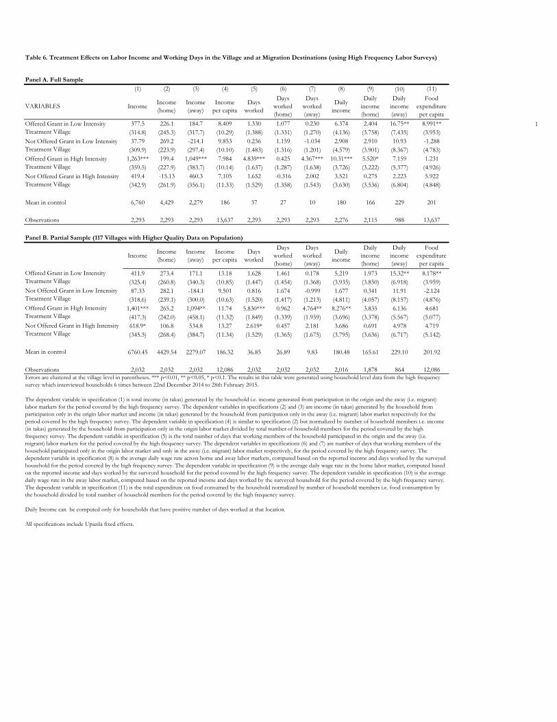
Errors are clustered at the village level in parentheses. *** p<0.01, ** p<0.05, * p<0.1. The results in this table were generated using household level data from the high frequency

survey which interviewed households 6 times between 22nd December 2014 to 28th February 2015.

The dependent variable in specification (1) is total income (in takas) generated by the household i.e. income generated from participation in the origin and the away (i.e. migrant)

labor markets for the period covered by the high frequency survey. The dependent variables in specifications (2) and (3) are income (in takas) generated by the household from

participation only in the origin labor market and income (in takas) generated by the household from participation only in the away (i.e. migrant) labor market respectively for the

period covered by the high frequency survey. The dependent variable in specification (4) is similar to specification (2) but normalized by number of household members i.e. income

(in takas) generated by the household from participation only in the origin labor market divided by total number of household members for the period covered by the high

frequency survey. The dependent variable in specification (5) is the total number of days that working members of the household participated in the origin and the away (i.e.

migrant) labor markets for the period covered by the high frequency survey. The dependent variables in specifications (6) and (7) are number of days that working members of the

household participated only in the origin labor market and only in the away (i.e. migrant) labor market respectively, for the period covered by the high frequency survey. The

dependent variable in specification (8) is the average daily wage rate across home and away labor markets, computed based on the reported income and days worked by the surveyed

household for the period covered by the high frequency survey. The dependent variable in specification (9) is the average daily wage rate in the home labor market, computed based

on the reported income and days worked by the surveyed household for the period covered by the high frequency survey. The dependent variable in specification (10) is the average

daily wage rate in the away labor market, computed based on the reported income and days worked by the surveyed household for the period covered by the high frequency survey.

The dependent variable in specification (11) is the total expenditure on food consumed by the household normalized by number of household members i.e. food consumption by

the household divided by total number of household members for the period covered by the high frequency survey.

Daily Income can be computed only for households that have positive number of days worked at that location.


Table 6. Treatment Effects on Labor Income and Working Days in the Village and at Migration Destinations (using High Frequency Labor Surveys)


Treatment Village


Treatment Village


Treatment Village


Treatment Village


Treatment Village


Treatment Village


Treatment Village


Treatment Village

(1) (2) (3) (4) (5) (6) (7) (8) (9) (10) (11)


(home)

Income

(away)

Income

per capita

Days

worked

Days

worked

(home)

Days

worked

(away)

Daily

income

Daily

income

(home)

Daily

income

(away)

Food

expenditure

per capita

206.8 247.2 -14.97 9.125 0.779 1.117 -0.404 4.635 2.651 14.09** 3.895

(272.6) (198.6) (271.5) (9.091) (1.216) (1.144) (1.103) (3.935) (3.412) (6.307) (4.095)

912.2*** 110.3 803.9** 7.620 3.513** 0.117 3.382** 7.489** 3.319 5.337 3.169

(307.9) (215.2) (331.3) (9.488) (1.425) (1.168) (1.421) (3.261) (2.980) (5.012) (4.394)

Mean in control 6,760.45 4,429.54 2,279.07 186.32 36.85 26.89 9.83 180.48 165.61 229.10 201.92

Observations 2,293 2,293 2,293 13,637 2,293 2,293 2,293 2,276 2,115 988 13,637

Upazila FE YES YES YES YES YES YES YES YES YES YES YES

Low Intensity Treatment

Village

High Intensity Treatment

Village

Table 7. Treatment Effects on Employment Outcomes using Village-Level Treatment Indicators (using High Frequency Labor Surveys)

Errors are clustered at the village level in parentheses. *** p<0.01, ** p<0.05, * p<0.1. The results in this table were generated using household level data from the high frequency survey which

interviewed households 6 times between 22nd December 2014 to 28th February 2015. These results complement the results in table 7. The dependent variables are the same as in table 7 but the

independent variables indicate village level treatment assignment. The sample includes all households surveyed in the high frequency survey i.e. households offered the travel grant and those not

offered the grant.

The dependent variable in specification (1) is total income (in takas) generated by the household i.e. income generated from participation in the origin and the away (i.e. migrant) labor markets

for the period covered by the high frequency survey. The dependent variables in specifications (2) and (3) are income (in takas) generated by the household from participation only in the origin

labor market and income (in takas) generated by the household from participation only in the away (i.e. migrant) labor market respectively for the period covered by the high frequency survey.

The dependent variable in specification (4) is similar to specification (2) but normalized by number of household members i.e. income (in takas) generated by the household from participation

only in the origin labor market divided by total number of household members for the period covered by the high frequency survey. The dependent variable in specification (5) is the total

number of days that working members of the household participated in the origin and the away (i.e. migrant) labor markets for the period covered by the high frequency survey. The dependent

variables in specifications (6) and (7) are number of days that working members of the household participated only in the origin labor market and only in the away (i.e. migrant) labor market

respectively, for the period covered by the high frequency survey. The dependent variable in specification (8) is the average daily wage rate across home and away labor markets, computed based

on the reported income and days worked by the surveyed household for the period covered by the high frequency survey. The dependent variable in specification (9) is the average daily wage

rate in the home labor market, computed based on the reported income and days worked by the surveyed household for the period covered by the high frequency survey. The dependent

variable in specification (10) is the total expenditure on food consumed by the household normalized by number of household members i.e. food consumption by the household divided by total

number of household members for the period covered by the high frequency survey.


(1) (2) (3) (4) (5) (6) (7) (8)

VARIABLES Migration Income Migration Income Savings Savings

All Income and

Profits (inclusive of

migration income)

All Income and

Profits (inclusive of

migration income)

All labor market

income (wages

earned at home and

destinations)

All labor market

income (wages

earned at home and

destinations)

Migrated 16,157*** 12,906*** -247.1 151.2 13,734** 7,030** 16,134*** 10,318***

(2,328) (1,621) (1,201) (690.9) (5,936) (2,999) (5,556) (2,804)

Observations 1,828 2,052 2,069 2,226 1,828 2,052 1,828 2,052

R-squared 0.479 0.447 0.008 0.021 0.006 0.045 0.099 0.145

SampleOnly Control

and Low-Intensity

Only Control

and High-Intensity

Only Control

and Low-Intensity

Only Control

and high-Intensity

Only Control

and Low-Intensity

Only Control

and High-Intensity

Only Control

and Low-Intensity

Only Control

and high-Intensity

1st-Stage Low-Intensity High-Intensity Low-Intensity High-Intensity Low-Intensity High-Intensity Low-Intensity High-Intensity

First stage partial R-squared 0.02 0.06 0.02 0.07 0.02 0.06 0.02 0.06

First stage F-test 15.70 55.56 19.50 79.30 15.70 55.56 15.70 55.56

First stage P-value 0.00 0.00 0.00 0 0.00 0.00 0.00 0.00

Table 8. LATE (IV) Estimates to Study the Differential Effects of Migration from Low-Intensity and High-Intensity Villages

Errors are clustered at the village level in parentheses. *** p<0.01, ** p<0.05, * p<0.1. The results in this table show IV specifications using household level data from the endline survey.

The dependent variable in specifications (1) and (2) are gross migration income; in specifications (3) and (4) are savings; in specifications (5) and (6) are all income (i.e. income from migration, income from home-labor market

participation and own-enterprise profits); and, are all labor market income (i.e. income from migration and income from home-labor market participation) reported by the household, accruing over the period September 15 2014 - April

30 2015. Specifications (1), (3), (5) and (7) restrict the analysis to only the control and low-intensity arms; specifications (2), (4), (6) and (8) restrict the analysis to only the control and high-intensity arms. There are a few massive outliers

in reported income, and all columns therefore trim out the extreme 1% of values for the dependent variable (top and bottom).

The dependent variable is regressed on a binary variable "Migrated" that takes on the value 1 if at least one member of household migrated during the relevant period and zero otherwise. This variable was instrumented in a 2SLS

regression using assignment to low-intensity or high-intensity treatment (as indicated). All specifications include Upazila fixed effects.

Panel A. Full Sample (Both High and Low Intensity Treatment Villages compared to Control)

(1) (2) (3) (4) (5) (6) (7) (8) (9) (10)


(home)

Income

(away)

Income

per capita

Days

worked

Days

worked

(home)

Days

worked

(away)

Daily

income

Daily

income

(home)

Food

expenditure

per capita

Migrated 8,255*** 555.3 7,549*** 33.18 31.54*** -0.446 32.01*** 59.32*** 26.24 12.59

(1,748) (1,483) (1,299) (95.25) (9.220) (7.888) (5.906) (20.41) (21.77) (43.43)

Observations 2,293 2,293 2,293 13,637 2,293 2,293 2,293 2,276 2,115 13,637

First stage partial R-squared 0.0141 0.0141 0.0141 0.00869 0.0141 0.0141 0.0141 0.0137 0.0131 0.00869

First stage F-test 4 4 4 3 4 4 4 3 3 3

First stage P-value 0 0 0 0 0 0 0 0 0 0

Panel B. Only High Intensity Treatment Villages Compared to Control Villages.

Migrated 9,135*** 1,787 7,171*** 93.19 34.15*** 3.971 29.67*** 80.05*** 51.16* 11.84

(2,452) (1,881) (1,567) (116.1) (11.89) (9.678) (6.953) (24.78) (29.44) (48.20)

Observations 1,644 1,644 1,644 9,769 1,644 1,644 1,644 1,629 1,516 9,769


First stage F-test 5.636 5.636 5.636 5.167 5.636 5.636 5.636 5.217 4.500 5.167

First stage P-value 0 0 0 0 0 0 0 0 0 0

Errors are clustered at the village level in parentheses. *** p<0.01, ** p<0.05, * p<0.1. The results in this table show a set of IV specifications that were generated using household level

data from the high frequency survey which interviewed households 6 times between 22nd December 2014 to 28th February 2015. The data across six rounds of surveys are pooled. Labor

income is measured as total income (in takas) generated by all household members participating in the labor market in their the origin village or away from the village for the period

covered by the high frequency origin survey (HFOS). Specifications (2) and (3) break down income by location. The HFOS also allows to track the number of working days for all

household members. The "average daily income" divides home earnings by number of days worked at home, and approximates a wage rate earned by household members working in the

home village. HFOS also added just a few questions on food consumption in a few aggregate categories, and we report effects on the total expenditure on food per capita in the last

column.

"Migrated", the RHS variable is binary, and =1 if at least one member of household migrated during the entire period covered by HFOS. This variable is instrumented in a 2SLS

regression using assignment to treatment (High and Low Intensity, Offered and Non-offered). All specifications include Upazila fixed effects.

Table 9. LATE (IV) Estimates of the Effects of Migration on Labor Income and Days Worked in the Village and at Migration

Destinations (using High Frequency Labor Surveys)

Panel A. Both High and Low Intensity Treatment Villages compared to Control

(1) (2) (3) (4) (5) (6)

VARIABLES

Monthly Frequency of

downsizing meals, Average

Across Lean Season

Months (August-January)



Across Non-Lean Season

Months (January-August)



Across Lean Season








Across Lean Season






Share of eligible villagers who migrated in 2015-2016 -0.316 -0.388 -0.644* -0.677* -0.852** -0.778**

(0.284) (0.286) (0.373) (0.369) (0.376) (0.388)

Observations 3,088 3,191 2,448 2,540 2,156 2,244

R-squared 0.073 0.049 0.085 0.047 0.081 0.047

Mean 0.919 0.573 0.92 0.586 0.921 0.586

Upazila FE YES YES YES YES YES YES

Sample All 133 villages All 133 villages 117 villages 117 villages 100 villages 100 villages

First stage partial R-squared 0.35 0.35 0.327 0.33 0.32 0.32

First stage F-test 29.28 30.28 26.83 27.6 23.37 24.15

First stage P-value 0.00 0.00 0.00 0.00 0.00 0.00

Table Food Security 1. LATE(IV) Estimates of the Effects of Migration on Frequency of Meal Downsizing in the Village During Lean and Non-Lean Seasons

Errors are clustered at the village level in parentheses. *** p<0.01, ** p<0.05, * p<0.1.

The results in this table show a set of IV specifications that were generated using village level data from the 2016 follow-up survey. The independent variable throughout is the share of eligible villagers who migrated in 2015-2016,

instrumented by treatment assignment to high- or low-intensity villages (two excluded dummy variables).

Food insecurity is measured as follows. For every given month from mid-August 2015 to midAugust 2016, each household was asked how many days in that month any member of that household had to cut down on meal portions

or number of meals in a day: rarely (0-5 days) or more than that (6 days to the whole month). In our data, rarely is marked as "0" and more than that as "1". Averaged across each village, this gives a village-level measure of food

insecurity per month, where a higher score (from 0 to 1) represents more food insecurity (i.e. more hunger). For these tables, the monthly numbers were averaged across the lean months (mid-August 2015-mid-January 2016) and

nonlean months (mid-January 2016 to mid-August 2016), giving a measure of food insecurity in each village across these periods. Columns (1), (3) and (5) represent the lean month averages while (2), (4) and (6) represent the

nonlean averages. Columns (1) and (2) use the full sample of villages, columns (3) and (4) use the partial sample, where data on village population is of higher quality, and columns (5) and (6) use the compact sample,

which is the subset of villages for which we have the most consistent and precise data.

Panel B restricts the sample to the high intensity and control villages only.


(1) (2) (3) (4) (5) (6) (7) (8) (9) (10)

VARIABLES

Worry About

Having Enough

Food?

Eat Less

Preferred

Food?

Limit

Variety of

Foods?

Limit Meal

Portion

Sizes?

Reduce

Number of

Daily Meals?

Go 24 Hours

Without Eating?

Have no Food

at All in the

House?

Go to

Sleep

Hungry?

Borrow Food

from Others

or on Credit?

Sell an Animal to Buy Food?

Share of eligible villagers who migrated in 2015-2016 -1.508* -1.022* -0.00403 -0.964 -0.694 -0.0428 -0.0501 -0.255 0.885 0.875

(0.831) (0.567) (0.602) (0.598) (0.527) (0.066) (0.290) (0.354) (0.570) (0.729)

Observations 2679 2679 2679 2679 2679 2679 2671 2679 2679 1122

R-squared 0.089 0.124 0.124 0.071 0.067 0.007 0.028 0.037 0.044 0.024

Mean 2.884 2.814 2.843 2.503 2.133 0.038 0.397 0.589 1.829 2.23


First stage F-test 26.28 26.28 26.28 26.28 26.28 26.28 26.24 26.28 26.28 28.18

First stage P-value 0.00 0.00 0.00 0.00 0.00 0.00 0.00 0.00 0.00 0.00

How Many Times in the Last

12 Months Did Household

Members:

How Many Times in the Last Week Did Household Members:

Table Food Security 2. LATE(IV) Estimates of the Effects of Migration on Various Food Security Variables in the Village

Errors are clustered at the village level in parentheses. *** p<0.01, ** p<0.05, * p<0.1.

The results in this table show a set of IV specifications that were generated using village level data from the 2016 follow-up survey. The independent variable throughout is the share of eligible villagers who migrated in 2015-2016, instrumented by

treatment assignment to high- or low-intensity villages (two excluded dummy variables).

Each column represents the village-level average of answers to the questions shown in the columns, where "0" represents a "no" and "1" represents a "yes".

All these specifications use the partial sample of 117 villages, for which we have higher-quality data on village population (the denominator on the RHS).


(1) (2) (4) (3) (4) (5) (6) (7) (8)

VARIABLES

Male wage

for

agricultural

work

Male wage

for non-

agricultural

work

Ln(Male

wage)

Log of

male

agricultural

wage

Log of

male

non-

agricultural

wage

Log of

female

agricultural

wage

Log of

female

non-

agricultural

wage

Log of

male

agricultural

wage

Log of

male

non-

agricultural

wage

Proportion Eligible Migrated 50.77* -0.425 0.172 0.265* 0.0619 0.224 0.362 0.178* 0.00664

(30.23) (36.30) (0.122) (0.137) (0.151) (0.216) (0.245) (0.107) (0.110)

Observations 333 239 477 333 239 187 45 380 268

1st-StageHigh

Intensity

High

Intensity

High

Intensity

High

Intensity

High

Intensity

High

Intensity

High

Intensity

High

Intensity

High

Intensity

First stage partial R-squared 0.447 0.476 0.463 0.447 0.476 0.439 0.645 0.506 0.512

First stage F-test 48.09 44.11 53.06 48.09 44.11 25.97 24.06 66.24 47.13

First stage P-value 1.75e-09 9.53e-09 3.30e-10 1.75e-09 9.53e-09 6.37e-06 5.29e-05 0 2.64e-09

Sample Partial Partial Partial Partial Partial Partial Partial Full Full

Standard errors clustered at the village level reported in parentheses. *** p<0.01, ** p<0.05, * p<0.1. Uses data from the employer survey which interviewed agricultural and non-

agricultural employers across all villages in the sample, and asked about wages paid during the period of out-migration. The survey asked separately about male and female wages, and

about agricultural and non-agricultural wages.

The dependent variable is regressed on the proportion of the eligible population that migrated in each village. This was constructed as a ratio of total migrant households in a village

and total eligible households in a village. The number of eligible households was available based on previous census data. The total number of migrants was constructed using the

same data and formulas used in Table 1. The independent variable was intrumented with village level assignment to the high intensity treatment.


Table 10. LATE (IV) Estimates of the Effects of Emigration on Wages Paid in the Home Village as Reported by Employers

(1) (2) (3) (4) (5) (6) (7) (8) (9)


(home)

Income

(away)

Days

worked

Days

worked

(home)

Days

worked

(away)

Daily

income

Daily

income

(home)

Daily

income

(away)

-318.7 14.67 -351.8** -1.252 0.221 -1.615*** -11.44 -5.752 12.10

(203.4) (101.6) (152.3) (1.051) (0.763) (0.593) (8.483) (7.963) (13.28)

136.9 -18.84 133.3 0.574 -0.170 0.631 -6.091 -8.388 0.0824

(228.7) (90.62) (189.9) (1.085) (0.626) (0.774) (8.070) (7.464) (9.291)

Mean in control 2090.11 856.6759 1212.00 12.22064 6.901385 5.207064 149.1694 121.2275 232.1413

Observations 2,293 2,293 2,293 2,293 2,293 2,293 1,152 973 400

Upazila FE YES YES YES YES YES YES YES YES YES

Errors are clustered at the village level in parentheses. *** p<0.01, ** p<0.05, * p<0.1. The results in this table were generated using household level

data from the high frequency survey which interviewed households 6 times between 22nd December 2014 to 28th February 2015. The sample is

restricted to the contributions of only non-primary working members to each of the outcomes (dependent variables as described below).

The dependent variable in specification (1) is total income (in takas) generated by the non-primary working members i.e. income generated by non-

primary working members from participation in the origin and the away (i.e. migrant) labor markets for the period covered by the high frequency

survey. The dependent variables in specifications (2) and (3) are income (in takas) generated by non-primary working members from participation only

in the origin labor market and income (in takas) generated by non-primary working members from participation only in the away (i.e. migrant) labor

market respectively for the period covered by the high frequency survey. The dependent variable in specification (4) is similar to specification (2) but

normalized by number of household members i.e. income (in takas) generated by the household from participation only in the origin labor market

divided by total number of household members for the period covered by the high frequency survey. The dependent variable in specification (5) is the

total number of days that non-primary working members of the household participated in the origin and the away (i.e. migrant) labor markets for the

period covered by the high frequency survey. The dependent variables in specifications (6) and (7) are number of days that non-primary working

members of the household participated only in the origin labor market and only in the away (i.e. migrant) labor market respectively, for the period

covered by the high frequency survey. The dependent variable in specification (8) is the average daily wage rate across home and away labor markets,

computed based on the reported income and days worked by the non-primary working members for the period covered by the high frequency survey.

The dependent variable in specification (9) is the average daily wage rate in the home labor market, computed based on the reported income and days

worked by the non-primary working members for the period covered by the high frequency survey.


Table 11 Treatment Effects on Employment Outcomes Restricting Only to Contributions Made by Non-

primary Workers (using High Frequency Labor Surveys)

Low Intensity

Treatment Village

High Intensity

Treatment Village

Variable Control VillageLow Intensity Treatment

Village


Village

Income 0.78 0.84 0.81

Income (Home) 0.82 0.84 0.84

Income (Away) 0.57 0.72 0.69

Days Worked 0.75 0.81 0.79

Days Worked (Home) 0.79 0.80 0.81

Days Worked (Away) 0.57 0.72 0.68

Daily Income 0.78 0.81 0.80

DailyIncome (Home) 0.82 0.84 0.84

DailyIncome (Away) 0.88 0.92 0.91

The results in this table were generated using household level data from the high frequency survey which interviewed households 6 times between 22nd

December 2014 to 28th February 2015. The table presents the proportion of the primary worker's contribution to the total for 9 key labor market

outcomes for all households sampled.

The variable in row (1) is income (in takas) generated by the primary worker divided by total household income, for income generated from

participation in both the origin and the away (i.e. migrant) labor markets for the period covered by the high frequency survey. The variables in rows (2)

and (3) are income (in takas) generated by the primary worker divided by total household income from participation only in the origin labor market and

income (in takas) generated by the primary worker divided by total household income from participation only in the away (i.e. migrant) labor market

respectively for the period covered by the high frequency survey. The variable in row (4) is the total number of days worked by the primary worker

divided by the total number of days worked by the household, for working members of the household that participated in the origin and the away (i.e.

migrant) labor markets for the period covered by the high frequency survey. The variables in specifications (5) and (6) are number of days worked by the

primary worker divided by the total number of days worked by the household only in the origin labor market and only in the away (i.e. migrant) labor

market respectively, for the period covered by the high frequency survey. The variable in specification (7) is the average daily income earned by primary

working members divided by household daily income across home and away labor markets, computed based on the reported income and days worked

by the surveyed household for the period covered by the high frequency survey. The variables in rows (8) and (9) are the average daily income earned by

primary working members divided by household daily income only in the origin labor market and only in the away (i.e. migrant) labor market

respectively, computed based on the reported income and days worked by the surveyed household for the period covered by the high frequency survey.

Table 12. Proportion of Contribution to Employment Outcomes Made by the One Primary Worker in the

Household

VARIABLE Control VillageLow Intensity

Treatment Village

High Intensity

Treatment Village

Proportion of Time Migrant Spends Away 0.33 0.32 0.32

Number of Trips Migrant Makes 1.49 1.55 1.56

Probability that when one Ever-Migrant is Home Another

Randomly Chosen Ever-Migrant in the Same Village is Away0.75 0.76 0.75

The results in rows (1) and (2) of this table were generated using household level data from the endline survey, while results in row (3) were generated using

household level data from the high frequency survey.

Row (1) presents simple arithmetic means of the time that migrant members spend away as a proportion of the total time enquired about (over the period

September 15 2014 - April 30 2015) for all households in the endline sample. Row (2) presents simple arithmetic mean number of trips that migrant members

take (over the period September 15 2014 - April 30 2015) for all households in the endline sample. Row (3) presents the probability that, for a given household

in a given round of the interview with no members away, at least one other household within their village has a member away (i.e. a member who is migrant.

Table 13. Migrants' Time Spent Away, Number of Trips Taken and Probability of Another Migrant Being Away

(1) (2) (3)

VARIABLES Income (home) Days worked (home) Daily income (home)

59.76** 0.231* 3.745

(29.35) (0.128) (2.516)

88.03*** 0.349*** 4.776**

(28.47) (0.133) (2.408)

Mean in control 592.57 3.37 177.61

Observations 9,730 9,730 8,310

Upazila FE YES YES YES


using household level data from the high frequency survey which interviewed households 6 times between 22nd December 2014

to 28th February 2015. The sample is restricted to the contributions of only primary working members to each of the outcomes

and only employment outcomes at origin are studied (dependent variables as described below).

The dependent variable in specification (1) is total income (in takas) generated by the primary working member from

participation in the origin labor market for the period covered by the high frequency survey. The dependent variable in

specification (2) is the total number of days that the primary working member of the household participated in the origin labor

market for the period covered by the high frequency survey. The dependent variable in specification (3) is the average daily wage

rate in the home labor markets, computed based on the reported income and days worked by the primary working members for

the period covered by the high frequency survey.


Low Intensity Treatment Village

High Intensity Treatment Village

Table 14. Treatment Effects on Employment Outcomes Restricting Only to Contributions

Made by Primary Workers while at Home (using High Frequency Labor Surveys)

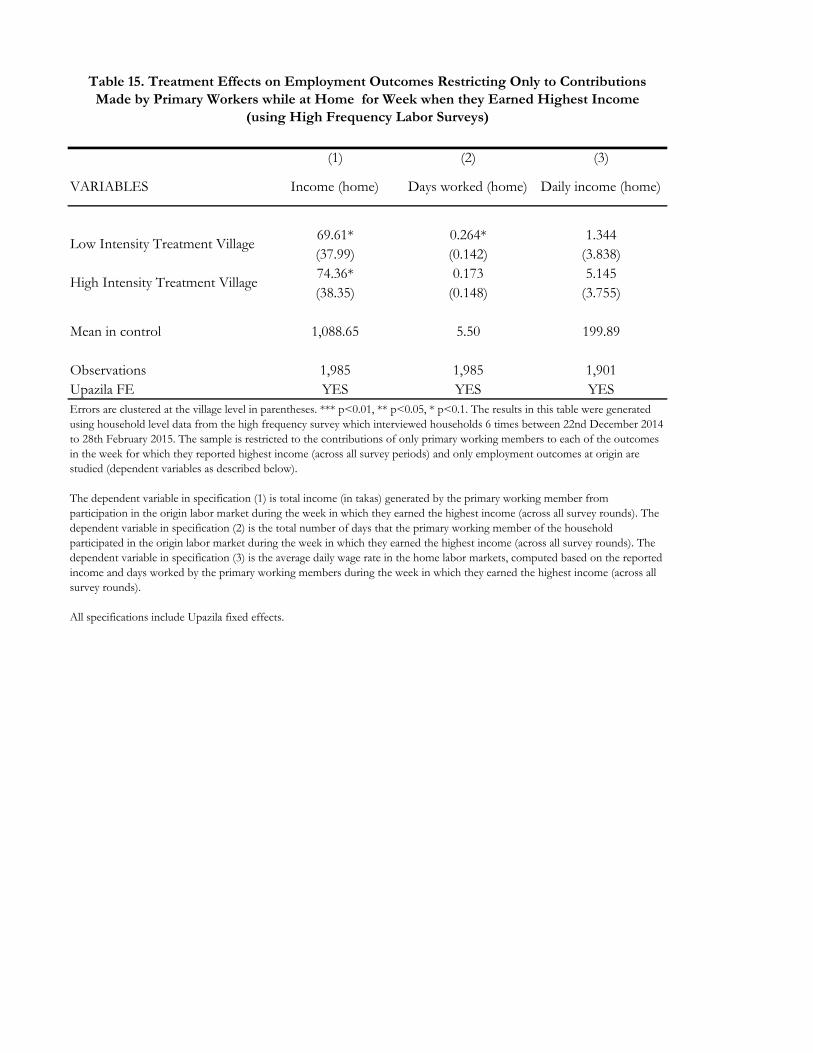
(1) (2) (3)

VARIABLES Income (home) Days worked (home) Daily income (home)

69.61* 0.264* 1.344

(37.99) (0.142) (3.838)

74.36* 0.173 5.145

(38.35) (0.148) (3.755)

Mean in control 1,088.65 5.50 199.89

Observations 1,985 1,985 1,901

Upazila FE YES YES YES

Low Intensity Treatment Village

High Intensity Treatment Village


using household level data from the high frequency survey which interviewed households 6 times between 22nd December 2014

to 28th February 2015. The sample is restricted to the contributions of only primary working members to each of the outcomes

in the week for which they reported highest income (across all survey periods) and only employment outcomes at origin are

studied (dependent variables as described below).

The dependent variable in specification (1) is total income (in takas) generated by the primary working member from

participation in the origin labor market during the week in which they earned the highest income (across all survey rounds). The

dependent variable in specification (2) is the total number of days that the primary working member of the household

participated in the origin labor market during the week in which they earned the highest income (across all survey rounds). The

dependent variable in specification (3) is the average daily wage rate in the home labor markets, computed based on the reported

income and days worked by the primary working members during the week in which they earned the highest income (across all

survey rounds).


Table 15. Treatment Effects on Employment Outcomes Restricting Only to Contributions

Made by Primary Workers while at Home for Week when they Earned Highest Income

(using High Frequency Labor Surveys)

(1) (2) (3) (1) (2) (3)

VARIABLESProfits per decimal

Aman 2015 (current)

Profits per decimal

Aman 2014

(previous)

Change in Profits per

decimal from 2013 to

2015

Profits per decimal

Aman 2015 (current)

Profits per decimal

Aman 2014

(previous)

Change in Profits per

decimal from 2013 to

2015

Share of eligible villagers who migrated in 2015-16 -254.9** -204.3* -19.55 -290.2** -234.8* -15.46

(124.8) (115.9) (72.23) (136.0) (134.9) (82.65)

Observations 626 626 626 547 547 547

Sample FULL FULL FULL PARTIAL PARTIAL PARTIAL

R-squared 0.086 0.088 0.040 0.095 0.092 0.041

Control Mean 83.361 95.842 -23.578 83.361 95.842 -23.578

Control Median 45.454 60 -18.399 45.454 60 -18.399

Firststage_R2partial 0.305 0.305 0.305 0.296 0.296 0.296

Firststage_Ftest 24.56 24.56 24.56 24.49 24.49 24.49

Firststage_Pvalue 8.94e-10 8.94e-10 8.94e-10 1.41e-09 1.41e-09 1.41e-09

Errors are clustered at the village level in parentheses. *** p<0.01, ** p<0.05, * p<0.1. The IV results in these tables were

generated with the 2016 Follow-up Employer Survey, combined with 2015 migration rates per village derived from the

2016 Follow-up Household Survey. Analysis is conducted at the village level. Uses data from the full sample of villages,

and results from the partial sample (with higher quality data on population) look very similar. All money-related variables

are measured in taka.

Dependent variables are all measures of profit (net revenues) per decimal (land unit) paid by the employer. Column (1)

measures this for 2015; column (2) for 2014; column (3) for 2013; column (4) measures the change in profits per decimal

from 2013 to 2014; column (5) measures the change in profits per decimal from 2013 to 2015.

The dependent variable is regressed on a binary variable "Migrated" that takes on the value 1 if at least one member of

household migrated during the relevant period and zero otherwise. This variable was instrumented in a 2SLS regression

using assignment to low-intensity or high-intensity treatment (as indicated). All specifications include Upazila fixed effects.


Table 16. LATE (IV) Estimates of the Effect of Emigration on Employer Profits

(1) (2) (3) (1) (2) (3)

VARIABLESRevenues per decimal

Aman 2015 (current)

Revenues per decimal

Aman 2014

(previous)


Aman 2013=>Aman

2015


Aman 2015 (current)


Aman 2014

(previous)


Aman 2013=>Aman

2015

Share of eligible villagers who migrated in 2015-16 -163.1 -183.5 -83.04 -133.8 -164.5 -102.6

(232.4) (220.2) (119.4) (272.4) (261.3) (144.9)

Observations 626 626 626 547 547 547

Sample FULL FULL FULL PARTIAL PARTIAL PARTIAL

R-squared 0.119 0.111 0.063 0.123 0.115 0.07

Control Mean 367.521 383.882 1.68 367.521 383.882 1.68

Control Median 254.545 294.193 -10.714 254.545 294.193 -10.714

Firststage_R2partial 0.305 0.305 0.305 0.296 0.296 0.296

Firststage_Ftest 24.56 24.56 24.56 24.49 24.49 24.49

Firststage_Pvalue 8.94e-10 8.94e-10 8.94e-10 1.41e-09 1.41e-09 1.41e-09


generated with the 2016 Follow-up Employer Survey, combined with 2015 migration rates per village derived from the 2016

Follow-up Household Survey. Analysis is conducted at the village level. Uses data from the full sample of villages, and results

from the partial sample (with higher quality data on population) look very similar. All money-related variables are measured in

taka.

Dependent variables are all measures of revenues per decimal (land unit) paid by the employer. Specification (1) has revenue per

decimal for 2015; specification (2) has this for 2014 and column (3) has the change in revenues per decimal from 2013 to 2015.


household migrated during the relevant period and zero otherwise. This variable was instrumented in a 2SLS regression using

assignment to low-intensity or high-intensity treatment (as indicated). All specifications include Upazila fixed effects.

Table 17. LATE (IV) Estimates of the Effect of Emigration on Employer Revenues

(1) (2) (3) (4) (5) (1) (2) (3) (4) (5)

VARIABLESCosts per decimal

(Aman 2015)

Costs per decimal

(Aman 2014)

Change in Costs per

decimal

from 2013 to 2015

Wage bill per

decimal

(Aman 2015)

Non-wage costs per

decimal

(Aman 2015)

Costs per decimal

(Aman 2015)

Costs per decimal

(Aman 2014)

Change in Costs per

decimal

from 2013 to 2015

Wage bill per

decimal

(Aman 2015)

Non-wage costs per

decimal

(Aman 2015)

Share of eligible villagers

who migrated in 2015-16145.6 58.48 224.1** 81.41 64.17 210.1 118.9 268.9** 93.78 116.3

(174.6) (165.1) (103.3) (79.42) (108.0) (214.8) (203.9) (124.8) (98.13) (132.3)

Observations 626 626 626 626 626 547 547 547 547 547

Sample FULL FULL FULL FULL FULL PARTIAL PARTIAL PARTIAL PARTIAL PARTIAL

R-squared 0.108 0.099 0.030 0.108 0.095 0.100 0.092 0.034 0.095 0.090

Control Mean 288.564 289.163 -25.507 149.011 139.553 288.564 289.163 -25.507 149.011 139.553

Control Median 232.33 231.481 4.962 122.125 103.634 232.33 231.481 4.962 122.125 103.634

Firststage_R2partial 0.305 0.305 0.305 0.305 0.305 0.296 0.296 0.296 0.296 0.296

Firststage_Ftest 24.56 24.56 24.56 24.56 24.56 24.49 24.49 24.49 24.49 24.49

Firststage_Pvalue 8.94e-10 8.94e-10 8.94e-10 8.94e-10 8.94e-10 1.41e-09 1.41e-09 1.41e-09 1.41e-09 1.41e-09


generated with the 2016 Follow-up Employer Survey, combined with 2015 migration rates per village derived from the

2016 Follow-up Household Survey. Analysis is conducted at the village level. Uses data from the full sample of villages,

and results from the partial sample (with higher quality data on population) look very similar. All money-related variables

are measured in taka.

Dependent variables in the first three specifications are all measures of costs per decimal (land unit) paid by the employer.

Column (1) has cost per decimal for 2015; specification (2) has this for 2014 and specificaiton (3) has the change in costs

per decimal from 2013 to 2015. The dependent variable in specificaiton (4) is wage per decimal (land unit) paid by the

employer in 2015 (including labor costs of land preparation, sowing, maintenance and harvesting). The dependent variable

in specification (5) encompasses costs per decimal incurred by the employer non-wage costs.


household migrated during the relevant period and zero otherwise. This variable was instrumented in a 2SLS regression

using assignment to low-intensity or high-intensity treatment (as indicated). All specifications include Upazila fixed effects.

Table 18. LATE (IV) Estimates of the Effect of Emigration on Employer Costs

(1) (2) (3) (4) (5) (6) (7) (8) (9) (10)

VARIABLES Rice (kg) Flour (kg) Pulses (kg)Edible oil

(liter)Fish (kg) Meat (kg)

Egg

(per egg)Milk (liter) Salt (kg) Sugar (kg)

-0.258** 0.0366 -0.432 -0.108 0.206 0.829 0.0222 0.836** 0.0724 -0.360**

(0.103) (0.199) (0.757) (0.597) (3.146) (1.708) (0.226) (0.396) (0.0882) (0.147)

-0.176* -0.240 -0.315 0.916 8.122* 1.713 -0.114 0.000563 0.00832 0.0110

(0.0964) (0.197) (0.682) (0.683) (4.644) (1.967) (0.143) (0.435) (0.0919) (0.145)

Mean in control 31.62 33.37 101.53 110.84 209.88 113.96 8.66 39.56 10.72 46.51

Observations 2,374 2,374 2,374 2,374 2,374 2,374 2,374 2,374 2,374 2,374

Upazila FE YES YES YES YES YES YES YES YES YES YES

Low Intensity Treatment

Village


Village

Errors are clustered at the village level in parentheses. *** p<0.01, ** p<0.05, * p<0.1. The results in this table were generated using shopkeeper (grocery store) level data from

the endline survey which interviewed households 6 times between 22nd December 2014 to 28th February 2015. The dependent variable in each specification is the price per

unit of a given item of food in the local village market.


Table 19. Treatment Effects on Local Food Prices

Table A1. Randomization Balance on Observables at Baseline

Control

Low

Intensity

(L)

High

Intensity

(H)

L - C p-Value H - C p-Value Treat. - C p-Value

Baseline Characteristics for 100 Villages Inducted in 2008

86.55 62.44 64.18 -24.10* 0.05 -22.37 0.10 -23.25* 0.05

(11.01) (5.35) (7.86) (12.15) (13.43) (11.86)

33.73 32.29 37.12 -1.44 0.69 3.39 0.40 0.92 0.78

(2.49) (2.7) (3.23) (3.64) (4.04) (3.23)

156.70 150.18 160.97 -6.52 0.66 4.27 0.79 -1.21 0.93

(11.2) (9.69) (11.31) (14.69) (15.79) (13.32)

4.04 3.87 4.00 -0.17 0.12 -0.04 0.70 -0.10 0.26

(0.08) (0.08) (0.07) (0.11) (0.10) (0.09)

2161.77 1982.55 1975.06 -179.23* 0.08 -186.72* 0.07 -182.89** 0.05**

(82.94) (57.89) (58.94) (100.40) (101.00) (91.73)

2988.85 2863.19 3002.75 -125.66 0.23 13.89 0.89 -57.12 0.55

(86.08) (57.35) (56.85) (102.68) (102.40) (94.50)

91.95 71.91 81.05 -20.03* 0.07 -10.90 0.39 -15.55 0.14

(8.96) (5.98) (8.89) (10.69) (12.53) (10.33)

67.44 72.55 54.42 5.12 0.60 -13.02 0.12 -3.83 0.63

(6.44) (7.25) (5.12) (9.62) (8.16) (7.83)

140.70 137.15 150.45 -3.56 0.66 9.75 0.24 2.98 0.68

(5.98) (5.37) (5.79) (7.97) (8.25) (7.13)

30.12 28.80 29.26 -1.31 0.74 -0.86 0.82 -1.09 0.75

(3.14) (2.39) (2.07) (3.91) (3.73) (3.47)

924.15 952.88 962.29 28.72 0.55 38.14 0.42 33.34 0.42

(33.87) (34.37) (32.67) (47.90) (46.70) (40.94)

1,960.56 1,955.12 1,984.76 -5.44 0.89 24.20 0.53 9.13 0.79

(27.95) (30.43) (26.32) (41.02) (38.10) (34.17)

2,062.61 2,047.24 2,095.15 -15.36 0.71 32.54 0.39 8.22 0.81

(29.13) (29.2) (24.7) (40.94) (37.91) (34.64)

2.03 1.91 2.05 -0.12 0.11 0.02 0.76 -0.05 0.44

(0.06) (0.06) (0.04) (0.08) (0.07) (0.07)

2.01 1.94 1.95 -0.06 0.29 -0.05 0.35 -0.06 0.25

(0.05) (0.05) (0.04) (0.06) (0.05) (0.05)

1.90 1.78 1.83 -0.11 0.22 -0.07 0.45 -0.09 0.26

(0.07) (0.07) (0.06) (0.09) (0.09) (0.08)

0.76 0.80 0.78 0.03 0.53 0.02 0.74 0.03 0.59

(0.04) (0.04) (0.04) (0.05) (0.05) (0.05)

77.79 78.76 77.96 0.97 0.68 0.18 0.95 0.58 0.79

(1.86) (1.52) (1.8) (2.38) (2.56) (2.17)

58.51 59.27 59.31 0.76 0.73 0.80 0.72 0.78 0.68

(1.6) (1.5) (1.54) (2.17) (2.19) (1.90)

49.71 53.26 54.21 3.54 0.14 4.50* 0.06 4.02** 0.05**

(1.56) (1.81) (1.84) (2.37) (2.39) (2.00)

0.26 0.23 0.24 -0.04 0.20 -0.02 0.42 -0.03 0.23

(0.03) (0.02) (0.03) (0.03) (0.03) (0.03)

1.20 1.15 1.19 -0.06 0.15 -0.01 0.84 -0.03 0.35

(0.04) (0.03) (0.03) (0.04) (0.04) (0.03)

1.07 1.01 1.03 -0.06 0.41 -0.04 0.50 -0.05 0.40

(0.06) (0.05) (0.04) (0.07) (0.06) (0.06)

Calorie intake per person per day

Value of total purchased meat

consumed per HH per month

Value of total purchased milk-egg


Value of total purchased fish


Household size

Value of purchased food consumed

per HH per month

Monthly total food expenditure

Value of medical exp incurred for

males per HH per month


females per HH per month

Value of clothes and shoes in 3

months per HH

Value of edu exp in 3 months per

Montly total non-food expenditure

Total Calories (per person per day)

Number of males in HH

Number of females in HH

Number of children in HH aged 0-

18


18 attending school

Subjective expectation: Monga

occurrence this year

Subjective expectation: Can send

remittance from Dhaka

Subjective expectation: Will get

social network help in Dhaka

HH Head Education (1=Educated)

Number of Males Age>14

Number of Children Age<9

Table A1. (Continued) Randomization Balance on Observables at Baseline

Control

Low

Intensity

(L)

High

Intensity

(H)

L - C p-Value H - C p-Value Treat. - C p-Value

Baseline Characteristics for 33 Villages Inducted in 2011

18.39 18.87 11.10 0.48 0.94 -7.29 0.23 -3.40 0.56

(5.56) (4.57) (3.04) (6.83) (5.93) (5.77)

6.66 5.83 5.76 -0.83 0.75 -0.91 0.74 -0.87 0.73

(2.61) (0.9) (1.13) (2.56) (2.65) (2.47)

565.28 588.74 590.72 23.46 0.61 25.45 0.57 24.46 0.56

(43.52) (22.13) (17.21) (45.66) (43.53) (41.87)

4.20 4.05 4.11 -0.15 0.28 -0.09 0.47 -0.12 0.31

(0.12) (0.09) (0.06) (0.14) (0.12) (0.12)

602.76 631.21 619.53 28.45 0.58 16.76 0.73 22.62 0.62

(45.84) (28.23) (20.85) (50.62) (46.97) (45.09)

13.96 36.02 27.99 22.05*** 0.01** 14.03*** 0.01** 18.04*** 0.01**

(2.45) (5.64) (3.54) (6.02) (4.16) (4.02)

14.15 22.62 25.24 8.46 0.20 11.09* 0.07 9.77** 0.05**

(3.37) (5.63) (4.82) (6.38) (5.69) (4.75)

147.68 157.55 153.22 9.87 0.36 5.54 0.59 7.69 0.41

(9.12) (6.36) (5.77) (10.49) (10.15) (9.30)

32.07 42.62 36.22 10.55 0.18 4.15 0.60 7.33 0.31

(7.11) (3.83) (4.39) (7.56) (7.85) (7.09)

14,965.80 17,021.89 15,530.85 2,056.09 0.18 565.05 0.70 1,300.36 0.33

(1270.04) (889.74) (832.88) (1,464.33) (1,431.04) (1,306.78)

2.23 2.08 2.15 -0.15 0.24 -0.08 0.47 -0.12 0.30

(0.12) (0.07) (0.05) (0.12) (0.11) (0.11)

1.97 1.97 1.97 0.00 0.99 -0.00 0.98 -0.00 1.00

(0.12) (0.05) (0.05) (0.12) (0.12) (0.11)

4.10 3.94 4.08 -0.16 0.18 -0.02 0.84 -0.09 0.37

(0.1) (0.08) (0.07) (0.11) (0.10) (0.10)

4.10 3.94 4.08 -0.16 0.18 -0.02 0.84 -0.09 0.37

(0.1) (0.08) (0.07) (0.11) (0.10) (0.10)

37.58 38.74 36.84 1.17 0.79 -0.74 0.86 0.21 0.95

(3.43) (3.03) (2.9) (4.35) (4.26) (3.73)

57.37 53.00 52.29 -4.37 0.25 -5.08 0.12 -4.72 0.11

(2.36) (3.04) (2.27) (3.71) (3.12) (2.83)

48.84 45.23 46.81 -3.62 0.21 -2.03 0.55 -2.83 0.23

(1.38) (2.53) (3.08) (2.80) (3.30) (2.32)

0.15 0.28 0.30 0.13** 0.04** 0.16** 0.02** 0.14** 0.02**

(0.06) (0.04) (0.04) (0.06) (0.06) (0.05)

1.27 1.25 1.30 -0.01 0.79 0.03 0.46 0.01 0.82

(0.03) (0.05) (0.04) (0.05) (0.04) (0.04)

0.91 0.93 0.93 0.02 0.89 0.01 0.90 0.02 0.89

(0.11) (0.09) (0.06) (0.12) (0.11) (0.10)

Value of total purchased meat



18

Value of total purchased milk-egg


Value of total purchased fish


Household size

Value of purchased food consumed

per HH per month


males per HH per month


females per HH per month

Value of clothes and shoes in 3

months per HH

Value of edu exp in 3 months per

Montly total non-food expenditure

Number of males in HH

Number of females in HH

Number of Children Age<9


18 attending school

Subjective expectation: Monga

occurrence this year

Subjective expectation: Can send

remittance from Dhaka

Subjective expectation: Will get

social network help in Dhaka

HH Head Education (1=Educated)

Number of Males Age>14

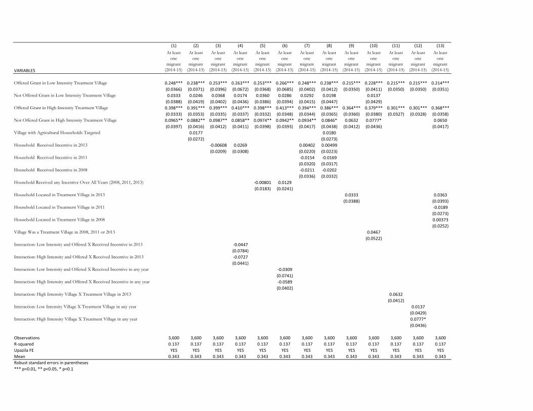
(1) (2) (3) (4) (5) (6) (7) (8) (9) (10) (11) (12) (13)

VARIABLES

At least

one

migrant

(2014-15)

At least

one

migrant

(2014-15)

At least

one

migrant

(2014-15)

At least

one

migrant

(2014-15)

At least

one

migrant

(2014-15)

At least

one

migrant

(2014-15)

At least

one

migrant

(2014-15)

At least

one

migrant

(2014-15)

At least

one

migrant

(2014-15)

At least

one

migrant

(2014-15)

At least

one

migrant

(2014-15)

At least

one

migrant

(2014-15)

At least

one

migrant

(2014-15)

Offered Grant in Low Intensity Treatment Village 0.248*** 0.238*** 0.253*** 0.263*** 0.253*** 0.266*** 0.248*** 0.238*** 0.215*** 0.228*** 0.215*** 0.215*** 0.214***

(0.0366) (0.0371) (0.0396) (0.0672) (0.0368) (0.0685) (0.0402) (0.0412) (0.0350) (0.0411) (0.0350) (0.0350) (0.0351)

Not Offered Grant in Low Intensity Treatment Village 0.0333 0.0246 0.0368 0.0174 0.0360 0.0286 0.0292 0.0198 0.0137

(0.0388) (0.0419) (0.0402) (0.0436) (0.0386) (0.0394) (0.0415) (0.0447) (0.0429)

Offered Grant in High Intensity Treatment Village 0.398*** 0.391*** 0.399*** 0.410*** 0.398*** 0.413*** 0.394*** 0.386*** 0.364*** 0.379*** 0.301*** 0.301*** 0.368***

(0.0333) (0.0353) (0.0335) (0.0337) (0.0332) (0.0348) (0.0344) (0.0365) (0.0360) (0.0380) (0.0327) (0.0328) (0.0358)

Not Offered Grant in High Intensity Treatment Village 0.0965** 0.0882** 0.0987** 0.0858** 0.0974** 0.0942** 0.0934** 0.0846* 0.0632 0.0777* 0.0650

(0.0397) (0.0416) (0.0412) (0.0411) (0.0398) (0.0393) (0.0417) (0.0438) (0.0412) (0.0436) (0.0417)

Village with Agricultural Households Targeted 0.0177 0.0180

(0.0272) (0.0273)

Household Received Incentive in 2013 -0.00608 0.0269 0.00402 0.00499

(0.0209) (0.0308) (0.0220) (0.0223)

Household Received Incentive in 2011 -0.0154 -0.0169

(0.0320) (0.0317)


(0.0336) (0.0332)

Household Received any Incentive Over All Years (2008, 2011, 2013) -0.00801 0.0129

(0.0183) (0.0241)

Household Located in Treatment Village in 2013 0.0333 0.0363

(0.0388) (0.0393)

Household Located in Treatment Village in 2011 -0.0189

(0.0273)

Household Located in Treatment Village in 2008 0.00373

(0.0252)

Village Was a Treatment Village in 2008, 2011 or 2013 0.0467

(0.0522)

Interaction: Low Intensity and Offered X Received Incentive in 2013 -0.0447

(0.0784)

Interaction: High Intensity and Offered X Received Incentive in 2013 -0.0727

(0.0441)

Interaction: Low Intensity and Offered X Received Incentive in any year -0.0309

(0.0741)

Interaction: High Intensity and Offered X Received Incentive in any year -0.0589

(0.0402)

Interaction: High Intensity Village X Treatment Village in 2013 0.0632

(0.0412)

Interaction: Low Intensity Village X Treatment Village in any year 0.0137

(0.0429)

Interaction: High Intensity Village X Treatment Village in any year 0.0777*

(0.0436)

Observations 3,600 3,600 3,600 3,600 3,600 3,600 3,600 3,600 3,600 3,600 3,600 3,600 3,600

R-squared 0.137 0.137 0.137 0.137 0.137 0.137 0.137 0.137 0.137 0.137 0.137 0.137 0.137

Upazila FE YES YES YES YES YES YES YES YES YES YES YES YES YES

Mean 0.343 0.343 0.343 0.343 0.343 0.343 0.343 0.343 0.343 0.343 0.343 0.343 0.343

Robust standard errors in parentheses

*** p<0.01, ** p<0.05, * p<0.1

(1) (2) (3) (4) (5) (6) (7) (8) (9) (10) (11) (12) (13)

VARIABLES

Migration

income

Migration

income

Migration

income

Migration

income

Migration

income

Migration

income

Migration

income

Migration

income

Migration

income

Migration

income

Migration

income

Migration

income

Migration

income

Offered Grant in Low Intensity Treatment Village 3,501*** 3,304*** 3,123** 3,842*** 3,317*** 3,883*** 2,909** 2,681* 2,259*** 3,525*** 2,259*** 2,259*** 2,263***

(846.40) (953.50) (1241.00) (1305.00) (1014.00) (1315.00) (1316.00) (1607.00) (843.40) (919.20) (843.40) (843.60) (850.10)Not Offered Grant in Low Intensity Treatment Village 1,242 1,071 985.5 1,017 1,142 1,192 653.4 456.6 1,267

(888.4) (1,044) (1,133) (1,042) (971.2) (921.7) (1,240) (1,513) (992.1)Offered Grant in High Intensity Treatment Village 5,093*** 4,954*** 4,982*** 4,849*** 5,093*** 4,888*** 4,738*** 4,582*** 3,851*** 5,117*** 3,656*** 3,656*** 3,910***

(904.30) (897.70) (842.50) (841.50) (904.40) (865.80) (836.60) (923.60) (1094.00) (953.00) (947.50) (947.00) (1085.00)Not Offered Grant in High Intensity Treatment Village 1,437* 1262.00 1277.00 1295.00 1,404* 1,422* 1046.00 848.00 195.20 1461.00 148.8

(783.60) (972.70) (875.60) (857.20) (791.70) (786.80) (923.20) (1215.00) (914.40) (888.90) (913.00)Village with Agricultural Households Targeted 351.5 386.2

(961.5) (994.8)Household Received Incentive in 2013 454.2 400.6 933.6 950.0

(968.0) (801.5) (1,170) (1,192)Household Received Incentive in 2011 -776.5 -808.9

(897.5) (923.6)Household Received Incentive in 2008 -845.7 -823.5

(816.3) (803.9)Household Received any Incentive Over All Years (2008, 2011, 2013) 313.2 165.8

(816.9) (604.2)Household Located in Treatment Village in 2013 1,242 1,130

(888.4) (984.0)Household Located in Treatment Village in 2011 -37.28

(805.9)Household Located in Treatment Village in 2008 597.8

(803.4)Village Was a Treatment Village in 2008, 2011 or 2013 -61.24

(1,210)Interaction: Low Intensity and Offered X Received Incentive in 2013 -789.2

(1,446)Interaction: High Intensity and Offered X Received Incentive in 2013 554.6

(2,675)Interaction: Low Intensity and Offered X Received Incentive in any year -557.3

(1,348)Interaction: High Intensity and Offered X Received Incentive in any year 786.7

(2,583)

Interaction: High Intensity Village X Treatment Village in 2013 195.2

(914.40)Interaction: Low Intensity Village X Treatment Village in any year 1,267

(992.10)Interaction: High Intensity Village X Treatment Village in any year 1,461

(888.90)

Observations 3,281 3,281 3,281 3,281 3,281 3,281 3,281 3,281 3,281 3,281 3,281 3,281 3,281

R-squared 0.046 0.046 0.046 0.046 0.046 0.046 0.046 0.047 0.046 0.046 0.046 0.046 0.046


Mean 5911.55 5911.55 5911.55 5911.55 5911.55 5911.55 5911.55 5911.55 5911.55 5911.55 5911.55 5911.55 5911.55


*** p<0.01, ** p<0.05, * p<0.1

Table A3. Robustness Checks on Effects of Migration on Migration Income

(1) (2) (3) (4) (5) (6) (7) (8) (9) (10) (11) (12) (13)

VARIABLES Income Income Income Income Income Income Income Income Income Income Income Income Income

Offered Grant in Low Intensity Treatment Village 382.9 544.5 594.7 1,898** 519.7 1,912** 585.6 762.3* 312.8 812.0** 312.8 315.2 311.7

(317.1) (355.8) (410.4) (761.3) (373.2) (758.0) (420.6) (452.8) (298.2) (369.0) (298.2) (298.3) (298.4)

Not Offered Grant in Low Intensity Treatment Village 70.16 232.1 197.8 -42.78 134.5 45.08 227.5 404.5 496.7

(314.2) (349.6) (342.0) (357.3) (327.4) (335.6) (356.9) (392.9) (361.8)

Offered Grant in High Intensity Treatment Village 1,222*** 1,343*** 1,292*** 1,383*** 1,236*** 1,399*** 1,319*** 1,450*** 1,152*** 1,636*** 707.4** 714.2** 1,163***

(341.8) (379.2) (354.0) (362.7) (342.6) (357.7) (352.2) (391.4) (350.9) (385.6) (316.7) (316.9) (345.9)

Not Offered Grant in High Intensity Treatment Village 514.9 659.6* 601.8* 434.9 542.9 500.0 628.8* 784.1** 444.7 921.5** 452.8

(330.9) (374.8) (340.0) (339.5) (333.0) (334.5) (340.4) (386.3) (343.4) (375.5) (347.5)

Village with Agricultural Households Targeted -320.3 -327.3

(322.6) (323.9)

Household Received Incentive in 2013 -233.0 196.9 -266.0 -283.3

(258.8) (308.7) (298.6) (295.0)


(309.7) (311.6)

Household Received Incentive in 2008 477.2 485.1

(356.2) (356.2)

Household Received any Incentive Over All Years (2008, 2011, 2013) -200.0 64.06

(228.5) (273.3)

Household Located in Treatment Village in 2013 70.16 98.17

(314.2) (324.4)

Household Located in Treatment Village in 2011 -172.6

(280.5)

Household Located in Treatment Village in 2008 36.22

(247.5)

Village Was a Treatment Village in 2008, 2011 or 2013 -987.0**

(435.4)

Interaction: Low Intensity and Offered X Received Incentive in 2013 -1,861**

(793.0)

Interaction: High Intensity and Offered X Received Incentive in 2013 -745.1

(503.7)

Interaction: Low Intensity and Offered X Received Incentive in any year -1,727**

(793.3)

Interaction: High Intensity and Offered X Received Incentive in any year -613.2

(501.0)

Interaction: Low Intensity Village X Treatment Village in 2013 444.7

(343.4)

Interaction: Low Intensity Village X Treatment Village in any year 496.7

(361.8)

Interaction: High Intensity Village X Treatment Village in any year 921.5**

(375.5)

Observations 2,249 2,249 2,249 2,249 2,249 2,249 2,249 2,249 2,249 2,249 2,249 2,249 2,249

R-squared 0.073 0.074 0.073 0.076 0.073 0.076 0.075 0.076 0.073 0.077 0.073 0.077 0.073


Mean 6853.37 6853.37 6853.37 6853.37 6853.37 6853.37 6853.37 6853.37 6853.37 6853.37 6853.37 6853.37 6853.37


*** p<0.01, ** p<0.05, * p<0.1

Table A4. Robustness Checks on Effects of Migration on Income (From High-Frequency Surveys)

(1) (2) (3) (4) (5) (6) (7) (8) (9) (10) (11) (12) (13)

VARIABLES

Away

Income

Away

Income

Away

Income

Away

Income

Away

Income

Away

Income

Away

Income

Away

Income

Away

Income

Away

Income

Away

Income

Away

Income

Away

Income

Offered Grant in Low Intensity Treatment Village 327.3 511.0 464.6 2,266** 413.0 2,316** 419.6 609.8 448.1 579.3 448.1 449.1 444.6

(319.7) (351.9) (411.5) (1,033) (369.4) (1,031) (416.8) (461.6) (288.4) (361.1) (288.4) (288.5) (288.2)Not Offered Grant in Low Intensity Treatment Village -120.8 62.36 -37.85 -361.6 -80.70 -195.0 -82.76 106.9 130.2

(290.5) (340.8) (327.2) (344.6) (305.9) (316.5) (330.2) (391.8) (331.9)Offered Grant in High Intensity Treatment Village 1,072*** 1,210*** 1,118*** 1,234*** 1,081*** 1,285*** 1,091*** 1,232*** 1,193*** 1,315*** 543.3 547.5* 1,128***

(360.3) (440.6) (378.5) (393.7) (362.1) (387.3) (373.7) (459.9) (405.3) (409.8) (328.2) (327.1) (385.3)Not Offered Grant in High Intensity Treatment Village 529.1 692.4* 586.6 357.5 547.1 490.1 565.6 731.6* 649.9* 767.6* 628.7*

(334.2) (391.2) (355.1) (348.7) (340.5) (340.5) (349.8) (414.5) (374.8) (390.2) (367.6)Village with Agricultural Households Targeted -362.8 -351.3

(383.8) (387.4)Household Received Incentive in 2013 -151.4 427.2 -93.42 -111.6

(275.0) (307.0) (306.1) (305.5)Household Received Incentive in 2011 -442.6 -416.3

(305.7) (309.9)Household Received Incentive in 2008 265.8 274.3

(353.6) (355.0)Household Received any Incentive Over All Years (2008, 2011, 2013) -126.7 215.8

(219.9) (240.7)Household Located in Treatment Village in 2013 -120.8 59.48

(290.5) (327.6)Household Located in Treatment Village in 2011 -307.0

(331.7)Household Located in Treatment Village in 2008 -360.8

(289.7)Village Was a Treatment Village in 2008, 2011 or 2013 -588.0*

(325.3)Interaction: Low Intensity and Offered X Received Incentive in 2013 -2,561**

(1,058)Interaction: High Intensity and Offered X Received Incentive in 2013 -980.9**

(495.2)Interaction: Low Intensity and Offered X Received Incentive in any year -2,350**

(1,051)Interaction: High Intensity and Offered X Received Incentive in any year -770.9

(484.5)Interaction: Low Intensity Village X Treatment Village in 2013 -120.8

(290.5)Interaction: High Intensity Village X Treatment Village in 2013 529.1

(334.2)Interaction: Low Intensity Village X Treatment Village in any year 130.2

(331.9)Interaction: High Intensity Village X Treatment Village in any year 767.6*

(390.2)

Observations 2,271 2,271 2,271 2,271 2,271 2,271 2,271 2,271 2,271 2,271 2,271 2,271 2,271

R-squared 0.052 0.053 0.052 0.057 0.052 0.057 0.053 0.054 0.052 0.054 0.052 0.054 0.055


Mean 2376.126 2376.126 2376.126 2376.126 2376.126 2376.126 2376.126 2376.126 2376.126 2376.126 2376.126 2376.126 2376.126


*** p<0.01, ** p<0.05, * p<0.1

Table A6. Robustness Checks on Effects of Migration on Away Income (From High-Frequency Surveys)

effects of emigration on rural labor markets may … · effects of emigration on rural labor...

Documents