International Trade and Labor Markets:

Unemployment, Inequality and Redistribution

A dissertation presented

by

Oleg Itskhoki

to

The Department of Economics

in partial fulfillment of the requirementsfor the degree of

Doctor of Philosophyin the subject of

Economics

Harvard UniversityCambridge, Massachusetts

April 2009

c© 2009 – Oleg Itskhoki

All rights reserved.

Dissertation Advisor: Professor Elhanan Helpman Oleg Itskhoki

International Trade and Labor Markets:

Unemployment, Inequality and Redistribution

International trade is typically believed to lead to aggregate welfare gains for trading

countries. However, it is also often viewed as a source of growing social disparity—by

causing unemployment and greater inequality within countries—which calls for an offset-

ting policy response. This dissertation consists of three theoretical essays studying these

issues.

The first chapter develops a model of international trade with labor market frictions

that differ across countries. We show that differences in labor market institutions con-

stitute a source of comparative advantage and lead to trade between otherwise similar

countries. Although trade ensures aggregate welfare gains for both countries, the more

flexible country stands to gain proportionately more. An increase in the country’s labor

market flexibility leads to welfare gains at home, but causes welfare losses in the trading

partner via decreased competitiveness of foreign firms. Trade can increase or decrease

unemployment by inducing an intersectoral labor reallocation generating rich patterns of

unemployment.

The second chapter proposes a new framework for thinking about the distributional

consequences of trade that incorporates firm and worker heterogeneity, search and match-

ing frictions in the labor market, and screening of workers by firms. Larger firms pay

higher wages and exporters pay higher wages than non-exporters. The opening of trade

enhances wage inequality and raises unemployment, but expected welfare gains are ensured

if workers are risk neutral. And while wage inequality is larger in a trade equilibrium than

in autarky, reductions of trade impediments can either raise or reduce wage inequality.

Conventional wisdom suggests that the optimal policy response to rising income in-

equality is greater redistribution. The final chapter studies an economy in which trade is

iii

associated with a costly entry into the foreign market, so that only the most productive

agents can profitably export. In this model, trade integration simultaneously leads to

rising income inequality and greater efficiency losses from taxation, both driven by the

extensive margin of trade. As a result, the optimal policy response may be to reduce the

marginal taxes, thereby further increasing inequality. In order to reap most of the welfare

gains from trade, countries may need to accept increasing income inequality.

iv

TABLE OF CONTENTS

Acknowledgments . . . . . . . . . . . . . . . . . . . . . . . . . . . . . . . . . . . . . vii

1. Labor Market Rigidities, Trade and Unemployment . . . . . . . . . . . . . . . . . 11.1 Introduction . . . . . . . . . . . . . . . . . . . . . . . . . . . . . . . . . . . . 11.2 The Model . . . . . . . . . . . . . . . . . . . . . . . . . . . . . . . . . . . . 5

1.2.1 Preferences and Demand . . . . . . . . . . . . . . . . . . . . . . . . . 61.2.2 Technologies and Market Structure . . . . . . . . . . . . . . . . . . . 71.2.3 Wages and Profits . . . . . . . . . . . . . . . . . . . . . . . . . . . . 91.2.4 Labor Market . . . . . . . . . . . . . . . . . . . . . . . . . . . . . . . 13

1.3 Equilibrium Structure . . . . . . . . . . . . . . . . . . . . . . . . . . . . . . 171.4 Trade, Welfare and Productivity . . . . . . . . . . . . . . . . . . . . . . . . 23

1.4.1 Welfare . . . . . . . . . . . . . . . . . . . . . . . . . . . . . . . . . . 231.4.2 Trade Structure . . . . . . . . . . . . . . . . . . . . . . . . . . . . . . 261.4.3 Productivity . . . . . . . . . . . . . . . . . . . . . . . . . . . . . . . 27

1.5 Unemployment . . . . . . . . . . . . . . . . . . . . . . . . . . . . . . . . . . 301.5.1 Symmetric Countries . . . . . . . . . . . . . . . . . . . . . . . . . . . 301.5.2 Asymmetric Countries . . . . . . . . . . . . . . . . . . . . . . . . . . 35

1.6 Firing Costs and Unemployment Benefits . . . . . . . . . . . . . . . . . . . 411.7 Concluding Comments . . . . . . . . . . . . . . . . . . . . . . . . . . . . . . 43

2. Inequality and Unemployment in a Global Economy . . . . . . . . . . . . . . . . 452.1 Introduction . . . . . . . . . . . . . . . . . . . . . . . . . . . . . . . . . . . . 452.2 Sectoral Equilibrium . . . . . . . . . . . . . . . . . . . . . . . . . . . . . . . 50

2.2.1 Model Setup . . . . . . . . . . . . . . . . . . . . . . . . . . . . . . . 502.2.2 Firm’s Problem . . . . . . . . . . . . . . . . . . . . . . . . . . . . . . 542.2.3 Sectoral Variables . . . . . . . . . . . . . . . . . . . . . . . . . . . . 582.2.4 Firm-specific Variables . . . . . . . . . . . . . . . . . . . . . . . . . . 62

2.3 Sectoral Wage Inequality . . . . . . . . . . . . . . . . . . . . . . . . . . . . . 652.4 Sectoral Unemployment . . . . . . . . . . . . . . . . . . . . . . . . . . . . . 732.5 Sectoral Income Inequality . . . . . . . . . . . . . . . . . . . . . . . . . . . . 772.6 General Equilibrium . . . . . . . . . . . . . . . . . . . . . . . . . . . . . . . 79

2.6.1 Outside Sector and Risk Neutrality . . . . . . . . . . . . . . . . . . . 802.6.2 Single Differentiated Sector and Risk Neutrality . . . . . . . . . . . 832.6.3 Outside Sector and Risk Aversion . . . . . . . . . . . . . . . . . . . 86

2.7 Conclusion . . . . . . . . . . . . . . . . . . . . . . . . . . . . . . . . . . . . 88

3. Optimal Redistribution in an Open Economy . . . . . . . . . . . . . . . . . . . . 913.1 Introduction . . . . . . . . . . . . . . . . . . . . . . . . . . . . . . . . . . . . 913.2 Closed Economy . . . . . . . . . . . . . . . . . . . . . . . . . . . . . . . . . 97

3.2.1 Economic Environment . . . . . . . . . . . . . . . . . . . . . . . . . 973.2.2 Optimal Redistribution in Closed Economy . . . . . . . . . . . . . . 101

3.3 Open Economy I: No Fixed Costs . . . . . . . . . . . . . . . . . . . . . . . . 1073.3.1 Properties of Open Economy Equilibrium . . . . . . . . . . . . . . . 1083.3.2 Optimal Redistribution . . . . . . . . . . . . . . . . . . . . . . . . . 112

3.4 Open Economy II: Fixed Costs of Trade . . . . . . . . . . . . . . . . . . . . 1143.4.1 Equilibrium Properties . . . . . . . . . . . . . . . . . . . . . . . . . . 1153.4.2 Optimal Linear Tax Rate . . . . . . . . . . . . . . . . . . . . . . . . 1193.4.3 Additional Tax Instruments . . . . . . . . . . . . . . . . . . . . . . . 123

3.5 Discussion . . . . . . . . . . . . . . . . . . . . . . . . . . . . . . . . . . . . . 130

Appendices 132

A. Appendices for Chapter I . . . . . . . . . . . . . . . . . . . . . . . . . . . . . . . 133A.1 Conditions for Incomplete Specialization . . . . . . . . . . . . . . . . . . . . 133A.2 Proof of Lemmas 1.1–1.5 and Proposition 1.3 . . . . . . . . . . . . . . . . . 134A.3 Derivation of results on productivity for Section 1.4.3 . . . . . . . . . . . . 135A.4 Solution under Pareto assumption for Section 1.5.2 . . . . . . . . . . . . . . 137

B. Appendices for Chapter II . . . . . . . . . . . . . . . . . . . . . . . . . . . . . . . 141B.1 Sectoral Equilibrium . . . . . . . . . . . . . . . . . . . . . . . . . . . . . . . 141

B.1.1 Symmetric Countries Closed Form Solutions . . . . . . . . . . . . . . 144B.2 Derivations and Proofs for Section 2.3 . . . . . . . . . . . . . . . . . . . . . 146B.3 Derivations and Proofs for Section 2.4 . . . . . . . . . . . . . . . . . . . . . 151B.4 Derivations and Proofs for Section 2.5 . . . . . . . . . . . . . . . . . . . . . 152B.5 Derivations and Proofs for Section 2.6 . . . . . . . . . . . . . . . . . . . . . 153B.6 Supplementary Derivations . . . . . . . . . . . . . . . . . . . . . . . . . . . 159

C. Appendices for Chapter III . . . . . . . . . . . . . . . . . . . . . . . . . . . . . . 162C.1 Derivations and Proofs for Section 3.2 . . . . . . . . . . . . . . . . . . . . . 162C.2 Results, Derivations and Proofs for Section 3.3 . . . . . . . . . . . . . . . . 166C.3 Derivations and Proofs for Section 3.3 . . . . . . . . . . . . . . . . . . . . . 173

Bibliography . . . . . . . . . . . . . . . . . . . . . . . . . . . . . . . . . . . . . . . . 179

vi

ACKNOWLEDGMENTS

I am extremely fortunately to have had the honor of working very closely with Elhanan

Helpman throughout my studies at Harvard: first as a student, then as a Teaching Fellow,

and finally as a co-author. His contribution to this dissertation is evident – two of the three

chapters of this dissertation are based on my joint work with Elhanan. It is impossible

to overstate how much I have learned from working with Elhanan over the past three

years. Learning-by-doing is extremely important in our profession, and I was privileged to

witness in real time how the highest quality academic research is done – something which

I believe is an absolutely essential part of academic training for any doctoral student.

My professional development would not be complete had it not been for Gita Gopinath,

another teacher and co-author. I have not included the research we have done with Gita

into this dissertation, but I am equally excited about it. Working with her helped me

acquire a very important complementary set of skills. I am also grateful to Steve Redding

and Roberto Rigobon, my two other co-authors, from whom I also learned a great deal.

I am very indebted to my advisor, Aleh Tsyvinski, for his guidance, support and all

his effort he put into me throughout my student years. Pol Antras’ advice and support

was also extremely important, especially his encouragement during the tough times of the

job market year.

I was very lucky to have come to Harvard at the time when a group of young profes-

sors joined the faculty, including Aleh Tsyvinski, Gita Gopinath, Pol Antras and Manuel

Amador. I have learned a great deal from them, both how to do outstanding economic

research and how to survive in the highly competitive environment of academic economics.

This experience is truly indispensable.

I also wish to thank Ken Rogoff and John Campbell whose exciting and very broad

research and most importantly their ability to link state-of-the-art theory with practice

and real-life problems provided inspiration in the beginning of my doctoral studies. I have

vii

also learned a lot from interactions with Philippe Aghion, Alberto Alesina, Robert Barro,

Emmanuel Farhi, Jordi Galı, Oliver Hart, Larry Katz, David Laibson, Greg Mankiw,

Nathan Nunn, Ariel Pakes, Andrei Shleifer, Jeremy Stein and Jim Stock. Finally, I was

very fortunate to have the invaluable experience of working as a Research Assistant for

Daron Acemoglu at MIT.

Part of the work on this dissertation was done at the Tel Aviv University, the Centre

for Economic Performance at the London School of Economics and at the Minneapolis

Fed. I thank these institutions for hospitality and productive academic environment.

I have had the privilege of studying at Harvard with a number of great future economists.

I wish to thank my TFs Ian Martin and Parag Pathak who provided a great example to

follow; my teaching colleagues Filipe Campante, Giacomo Ponzetto and Elias Albagli; my

office mates at different times Mihai Manea, Anthony Niblett and Thomas Baranga, and

many of my classmates from whom I learned a lot. I wish to separately acknowledge

and thank Loukas Karabarbounis, Matt Weinzierl and Elias Albagli for the very valuable

comments on my research.

Harvard has given me the opportunity to meet hundreds of interesting people and

make many great friends. Without their support the completion of this dissertation would

not have been possible. I should mention separately Lena and Sasha, Erdin and Ellen,

Artashes, and Keyu.

Finally, I thank my family—Mom and Dad, Olga, Dave and Max, and Grandma—for

their support, their belief in me, and their joy for my achievements.

To my Albina, for her love and patience!

viii

1. LABOR MARKET RIGIDITIES, TRADE AND UNEMPLOYMENT

(with Elhanan Helpman)

1.1 Introduction

International trade and international capital flows link national economies. Although

such links are considered to be beneficial for the most part, they produce an interdepen-

dence that occasionally has harmful effects. In particular, shocks that emanate in one

country may negatively impact trade partners. On the trade side, links through terms-of-

trade movements have been studied extensively, and it is now well understood that, say,

capital accumulation or technological change can worsen a trade partner’s terms of trade

and reduce its welfare. On the macro side, the transmission of real business cycles has

been widely studied, such as the impact of technology shocks in one country on income

fluctuations in its trade partners.

Although a large literature addresses the relationship between trade and unemploy-

ment, we fall short of understanding how these links depend on labor market rigidities.

Indeed, measures of labor market flexibility developed by Botero et al. (2004) differ greatly

across countries.1 The rigidity of employment index, which is an average of three other

indexes—difficulty of hiring, difficulty of firing, and rigidity of hours—shows wide vari-

ation in its range between zero and one hundred (where higher values represent larger

rigidities). Importantly, countries with very different development levels may have similar

labor market rigidities. For example, Chad, Morocco and Spain have indexes of 60, 63

and 63, respectively, which are about twice the average for the OECD countries (which

1 Their original data has been updated by the World Bank and is now available athttp://www.doingbusiness.org/ExploreTopics/EmployingWorkers/. The numbers reported in the textcome from this site, downloaded on May 20, 2007. Other measures of labor market characteristics areavailable for OECD countries; see Nickell (1997) and Blanchard and Wolfers (2000).

is 33.3) and higher than the average for sub-Saharan Africa. The United States has the

lowest index, equal to zero, while Australia has an index of three and New Zealand has an

index of seven, all significantly below the OECD average. Yet some of the much poorer

countries also have very flexible labor markets, e.g., both Uganda and Togo have an index

of seven.2

We develop in this paper a two-country model of international trade in order to study

the effects of labor market frictions on trade flows, productivity, welfare and unemploy-

ment. We are particularly interested in the impact of a country’s labor market rigidities

on its trade partner, and the differential impact of lower trade impediments on countries

with different labor market rigidities. Blanchard and Wolfers (2000) emphasize the need

to allow for interactions between shocks and differences in labor market characteristics

in order to explain the evolution of unemployment in European economies. They show

that these interactions are empirically important. On the other side, Nickell et al. (2002)

emphasize changes over time in labor market characteristics as important determinants

of the evolution of unemployment in OECD countries. We focus the analysis on search

and matching frictions in Sections 1.2-1.5, and discuss in Section 1.6 how the results

generalizations to economies with firing costs and unemployment benefits.3

The literature on trade and unemployment is large and varied. One strand of this lit-

erature considers economies with minimum wages, of which Brecher (1974) represents an

early contribution.4 Another approach, due to Matusz (1986), uses implicit contracts. A

third approach, exemplified by Copeland (1989), incorporates efficiency wages into trade

models. Yet another line of research uses fair wages. Agell and Lundborg (1995) and

Kreickemeier and Nelson (2006) illustrate this approach. The final approach uses search

and matching in labor markets. While two early studies (Davidson, Martin and Matusz,

2 There is growing awareness that institutions affect comparative advantage and trade flows. Levchenko(2007), Nunn (2007) and Costinot (2006) provide evidence on the impact of legal institutions, while Cunatand Melitz (2007) and Chor (2006) provide evidence on the impact of labor market rigidities.

3 While we use a static specification of labor market frictions, our analysis is consistent with a steadystate of a dynamic model as we show in Helpman and Itskhoki (2009).

4 His approach has been extended by Davis (1998) to study how wages are determined when two countriestrade with each other, one with and one without a minimum wage.

2

1988, and Hosios, 1990) extended the two-sector model of Jones (1965) to economies with

this type of labor market friction, Davidson, Martin and Matusz (1999) provide a particu-

larly valuable analysis of international trade with labor markets that are characterized by

Diamond-Mortensen-Pissarides-type search and matching frictions (see Pissarides, 2000,

for the theory of search and matching in labor markets). In their model differences in

labor market frictions, both across sectors and across countries, generate Ricardian-type

comparative advantage.

Our two-sector model incorporates Diamond-Mortensen-Pissarides-type frictions into

both sectors; one producing homogenous goods, the other producing differentiated prod-

ucts. In both sectors wages are determined by bargaining. There is perfect competition

in homogeneous goods and monopolistic competition in differentiated products. In the

differentiated-product sector firms are heterogeneous, as in Melitz (2003). These firms

exercise market power in the product market on the one hand, and bargain with workers

over wages on the other.5 Moreover, there are fixed and variable trade costs in the dif-

ferentiated sector. We focus the analysis on the differentiated sector and think about the

homogeneous sector as the rest of the economy. The analysis generalizes in a straightfor-

ward way to the case of multiple differentiated sectors.

We develop the model in stages. The next section describes demand, product markets,

labor markets, and the determinants of wages and profits. In the following section, Section

1.3, we discuss the structure of equilibrium, focusing on the case in which both countries

are incompletely specialized, and—as in Melitz (2003)—only a fraction of firms export in

the differentiated-product industry and some entrants exit this industry. This is followed

by an analysis of the impact of labor market frictions on trade, welfare, and productivity in

Section 1.4. We allow the labor market frictions to vary both across countries and sectors.

There we also study the differential impact of lower trade impediments on countries with

5 A surge of papers has incorporated labor market frictions into models with heterogeneous firms. Eggerand Kreickemeier (2009) examine trade liberalization in an environment with fair wages and Davis andHarrigan (2007) examine trade liberalization in an environment with efficiency wages; both papers focuson the wage dispersion of identical workers across heterogeneous firms in symmetric countries. Mitra andRanjan (2007) examine offshoring in an environment with search and matching and Felbermayr, Prat andSchmerer (2008) study trade in a one-sector model with search and matching and symmetric countries.

3

different labor market frictions. Importantly, we show that both countries gain from

trade in welfare terms and in terms of total factor productivity, independently of trade

costs and differences in labor market rigidities. The lowering of labor market frictions in

the differentiated sector of one country raises its welfare, but harms the trade partner.

Nevertheless, both countries benefit from simultaneous proportional reductions of labor

market frictions in the differentiated sector across the world.

By lower frictions in its differentiated sector’s labor market a country gains a compet-

itive advantage in this sector, which is reminiscence of a productivity improvement (but

not identical). As a result, it attracts more firms into this sector while the foreign country

attracts fewer firms. The entry and exit of firms overwhelms the terms of trade movement,

leading to welfare gains in the country with improved labor market frictions and welfare

losses in its trade partner.

In Section 1.4 we also show that labor market flexibility is a source of comparative

advantage. The country with relatively lower labor market frictions in the differentiated

sector (i.e., lower relative to the homogeneous sector) has a larger fraction of exporting

firms and it exports differentiated products on net. Moreover, the share of intra-industry

trade is smaller while the volume of trade is larger the larger is the difference in relative

sectoral labor market rigidities across countries.

In Section 1.5 we take up unemployment. We show that the relationship between un-

employment and labor market rigidity in the differentiated sector is hump-shaped when

the countries are symmetric. A decline in labor market frictions in the differentiated sector

decreases the sectoral rate of unemployment and induces more workers to search for jobs

in the differentiated-product sector. When the differentiated sector has the lower sectoral

rate of unemployment, which happens when labor market frictions are relatively lower in

this sector, the reallocation of workers across sectors, i.e., the composition effect, reduces

the aggregate rate of unemployment. Under these circumstances the aggregate rate of

unemployment declines, because both the shift in the sectoral rate of unemployment and

the reallocation of workers across sectors reduce the aggregate rate of unemployment. On

the other hand, when labor market frictions are higher in the differentiated sector, these

4

two effects impact unemployment in opposite directions, with the composition effect dom-

inating in a highly rigid labor market and the sectoral unemployment effect dominating

in a mildly rigid labor market. As a result, unemployment initially increases and then

decreases as labor market frictions decline, starting from high levels of rigidity.

We also discuss the transmission of shocks across asymmetric countries, using numer-

ical examples to illustrate various patterns. In particular, we show that in the absence

of unemployment in the homogenous sector, if a single country reduces its labor market

frictions in the differentiated sector this reduces unemployment in the country’s trading

partner by inducing a labor reallocation from the differentiated-product sector to the

homogeneous-product sector. We also show that lowering trade impediments can increase

unemployment in one or both countries, despite its positive welfare effect, and that the

interaction between trade impediments and labor market rigidities produces rich patterns

of unemployment. Specifically, differences in rates of unemployment across countries do

not necessarily reflect differences in labor market frictions; the more flexible country can

have higher or lower unemployment, depending on the height of trade impediments and

the levels of labor market frictions.

In Section 1.6 we discuss the impacts of firing costs and unemployment benefits as

additional sources of labor market frictions. In particular, we describe conditions under

which the previous results remain valid, as well as how they change when these conditions

are not satisfied. The last section summarizes some of the main insights from this analysis.

1.2 The Model

We develop in this section the building blocks of our analytical model. They consist of

a demand structure, technologies, product and labor market structures, and determinants

of wages and profits. After describing these ingredients in some detail, we discuss in the

next three sections equilibrium interactions in a two-country world. In order to focus on

labor market rigidities, we assume that the two countries are identical except for labor

market frictions. This means that the demand structure and the technologies are the same

in both countries. They can differ in the size of their labor endowment, but this difference

5

is not consequential for the type of equilibrium we discuss in the main text.

1.2.1 Preferences and Demand

Every country has a representative agent who consumes a homogeneous product q0

and a continuum of brands of a differentiated product whose real consumption index is

Q. The real consumption index of the differentiated product is a constant elasticity of

substitution aggregator:

Q =[∫

ω∈Ωq(ω)βdω

] 1β

, 0 < β < 1, (1.1)

where q (ω) represents the consumption of variety ω, Ω represents the set of varieties

available for consumption, and β is a parameter that controls the elasticity of substitution

between brands.

Consumer preferences between the homogeneous product, q0, and the real consumption

index of the differentiated product, Q, are represented by the quasi-linear utility function6

U = q0 +1ζQζ , 0 < ζ < β.

The restriction ζ < β ensures that varieties are better substitutes for each other than for

the outside good q0. We also assume that the consumer has a large enough income level

to always consume positive quantities of the outside good, in which case it is convenient

to choose the outside good as numeraire, so that its price equals one, i.e., p0 = 1. Under

the circumstances p (ω), the price of brand ω, and P , the price index of the brands, are

measured relative to the price of the homogeneous product.

The utility function U implies that a consumer with spending E who faces the price

index P for the differentiated product chooses Q = P−1/(1−ζ) and q0 = E − P−ζ/(1−ζ).7

6 Alternatively, we could use a homothetic utility function in q0 and Q (see Chapter II).

7 The assumption that consumer spending on the outside good is positive is equivalent to assumingE > P−ζ/(1−ζ). Since ζ > 0, the demand for Q is elastic and total spending PQ rises when P falls.

6

As a result, the demand function for brand ω can be expressed as

q(ω) = Q−β−ζ

1−β p(ω)−1

1−β (1.2)

and the indirect utility function as

V = E +1− ζζ

P− ζ

1−ζ = E +1− ζζ

Qζ . (1.3)

As usual, the indirect utility function is increasing in spending and declining in price. A

higher price index P reduces the demand for Q, and—holding expenditure E constant—

reduces welfare. This decline in welfare results from the fact that consumer surplus,

(1− ζ)P−ζ/(1−ζ)/ζ = (1− ζ)Qζ/ζ, declines as P rises and Q falls. In what follows, we

characterize equilibrium values of Q, from which we infer welfare levels.

1.2.2 Technologies and Market Structure

All goods are produced with labor, which is the only factor of production. The market

for the homogeneous product is competitive, and this good serves as numeraire, so that

p0 = 1. When a firm is matched with a worker, they produce one unit of the homogenous

good.

The market for brands of the differentiated product is monopolistically competitive.

A firm that seeks to supply a brand ω bears an entry cost fe in terms of the homogeneous

good, which covers the technology cost and the cost of setting up shop in the industry.

After bearing this cost, the firm learns how productive its technology is, as measured by

θ; a θ-firm requires 1/θ workers per unit output. In other words, if a θ-firm employs h

workers it produces θh units of output. Before entry the firm expects θ to be drawn from

a known cumulative distribution Gθ (θ).

After entry the firm has to bear a fixed production cost fd in terms of the homogeneous

good; without it no manufacturing is possible. Following Melitz (2003), we assume that the

differentiated-product sector bears a fixed cost of exporting fx in terms of the homogeneous

product. In addition, it bears a variable cost of exporting of the melting-iceberg type:

7

τ > 1 units have to be exported for one unit to arrive in the foreign country.8

We label the two countries A and B. If a country-j firm, j = A,B, with productivity

θ hires hj workers and chooses to serve only the domestic market, then (1.2) implies that

its revenue equals

Rj = Q−(β−ζ)j Θ1−βhβj ,

where Θ ≡ θβ/(1−β) is a transformed measure of productivity that is more convenient for

our analysis. Higher Qj implies tighter competition in the differentiated product market

of country-j and proportionately reduces revenues for all firms serving this market.

If, instead, this firm chooses also to export, then it has to allocate output θhj across

the domestic and foreign markets, i.e., θhj = qdj + qxj , where qdj represents the quantity

allocated to the domestic market and qxj represents the quantity allocated to the export

market.9 With an optimal allocation of output across markets, the resulting total revenue

is

Rj =[Q−β−ζ

1−βj + τ

− β1−βQ

−β−ζ1−β

(−j)

]1−βΘ1−βhβj ,

where (−j) is the index of the country other than j. In general, the revenue function of

8 As is common in models with home market effects, we assume that there are no trade frictions in thehomogeneous-product sector. We show in our working paper Helpman and Itskhoki (2008) that addingtrade costs to the homogenous sector does not affect the results when these costs are not too large. Inthat paper there are no labor market frictions in the homogenous sector, but the same arguments can beadapted to our framework.

9 From (1.2) these quantities have to satisfy

qdj = Q− β−ζ1−βj p

− 11−β

dj and qxj = τQ− β−ζ1−β(−j) (τpxj)

− 11−β .

In this specification pdj and pxj are producer prices of home and foreign sales, respectively. Note thatwhen exports are priced at pxj , consumers in the foreign country pay an effective price of τpxj due to the

variable export costs. Under the circumstances they demand Q−(β−ζ)/(1−β)

(−j) (τpxj)−1/(1−β) consumption

units. To deliver these consumption units the supplier has to manufacture qxj units, as shown above. Sucha producer maximizes total revenue when marginal revenues are equalized across markets. In the case ofconstant elasticity of demand functions this requires equalization of producer prices, which implies thatthe optimal allocation of output satisfies

qxj/qdj = τ− β

1−β(Q(−j)/Qj

)− β−ζ1−β .

8

country-j firm with productivity θ can therefore be represented by

Rj (Θ, hj) =[Q−β−ζ

1−βj + Ixj (Θ) τ−

β1−βQ

−β−ζ1−β

(−j)

]1−βΘ1−βhβj , (1.4)

where Ixj (Θ) is an indicator variable that equals one if the firm exports and zero otherwise.

1.2.3 Wages and Profits

There are search and matching frictions in every sector and firms post vacancies in

order to attract workers. The cost of posting vacancies and the matching process generate

hiring costs. Moreover, search and matching frictions generate bilateral monopoly power

between a worker and his firm, as a result of which they engage in wage bargaining.10

We assume that in the homogeneous-product sector every firm employs one worker.

This assumption is common in the search and matching literature (see Pissarides, 2000)

and in our case leads to no loss of generality. Since firms in this sector are homogenous

in terms of productivity and produce a homogenous good, our analysis does not change if

we allow firms to hire multiple workers, as long as they remain price takers.

When a firm and a worker match, they bargain over the surplus from the relationship.

Since the outside option of each party equals zero at this stage, the surplus—which consists

of the revenue from sales of one unit of the homogeneous product—equals one. Assuming

equal weights in the bargaining game then implies that the worker gets a wage w0 = 1/2

and the firm gets a profit π0 = 1/2, and these payoffs are the same in every country. We

discuss additional details of the labor market equilibrium in this sector in the following

section.

In the differentiated-product industry firms are heterogeneous in terms of productivity

but face the same cost of hiring in the labor market. A Θ-firm from country j that seeks

to employ hj workers bears the hiring cost bjhj in terms of the homogeneous good, where

bj is exogenous to the firm yet it depends on sectoral labor market conditions, as we

10 In the earlier working paper version (Helpman and Itskhoki, 2008), we focused on the case in whichthere are no labor market frictions in the homogeneous-product sector. The current framework incorporatesit as a special case (see footnote 15).

9

discuss below. It follows that a worker cannot be replaced without cost. Under these

circumstances, a worker inside the firm is not interchangeable with a worker outside the

firm, and workers have bargaining power after being hired. Workers exploit this bargaining

power in the wage determination process.

We assume that the hj workers and the firm engage in strategic wage bargaining with

equal weights in the manner suggested by Stole and Zwiebel (1996a,b), which is a natural

extension of Nash bargaining to the case of multiple workers. The revenue function (1.4)

then implies that the firm gets a fraction 1/ (1 + β) of the revenue and the workers get a

fraction β/ (1 + β).11 Recall that β determines the concavity of the revenue function in

the number of workers; a lower β makes the revenue more concave and reduces the revenue

loss from the departure of a marginal worker. Therefore, lower β reduces the equilibrium

share of the workers in the division of revenue. This bargaining outcome is derived under

the assumption that at the bargaining stage a worker’s outside option is unemployment,

and the value of unemployment is zero because there are no unemployment benefits and

the model is static. In Section 1.6 we discuss unemployment benefits, and in Helpman

and Itskhoki (2009) we show that our bargaining solution carries over to the steady state

of a dynamic model.

Anticipating the outcome of this bargaining game, a Θ-firm that wants to stay in

the industry chooses an employment level, hj , and whether to serve the foreign market,

Ixj ∈ 0, 1, that maximize profits. That is, it solves the following problem:

πj(Θ) ≡ maxIxj∈0,1,hj≥0.

1

1 + β

[Q−β−ζ

1−βj + Ixjτ

− β1−βQ

−β−ζ1−β

(−j)

]1−βΘ1−βhβj − bjhj − fd − Ixjfx

.

(1.5)

11 In the solution to the Stole and Zwiebel bargaining game the firm and a worker equally divide themarginal surplus from their relationship, i.e.,

∂

∂h

[Rj(Θ, h)− wj(Θ, h)h

]= wj(Θ, h),

where wj(Θ, h) is the bargained wage rate in a Θ-firm in country-j which employs h workers. Therefore,the left-hand side represents the surplus of the firm from employing the marginal worker, accounting forthe fact that his departure will impact the wage rate of the remaining workers. The wage on the right-hand side is the worker’s surplus. Using the expression for revenue (1.4), the above condition represents adifferential equation for the wage schedule which yields the solution wj(Θ, h) = β/(1 + β) ·Rj(Θ, h)/h.

10

The solution to this problem implies that the employment level of a Θ-firm in country j

can be decomposed into

hj (Θ) = hdj (Θ) + Ixj (Θ)hxj (Θ) ,

where hdj (Θ) represents employment for domestic sales, hxj (Θ) represents employment

for export sales, and

hdj (Θ) = φ1β

1 b− 1

1−βj Q

−β−ζ1−β

j Θ,

hxj (Θ) = φ1β

1 b− 1

1−βj τ

− β1−βQ

−β−ζ1−β

(−j) Θ,

(1.6)

where

φ1 =(

β

1 + β

) β1−β

.

Furthermore, a country-j firm with productivity Θ pays wages

wj (Θ) =β

1 + β

Rj (Θ)hj (Θ)

= bj , (1.7)

where the first equality is the outcome of the bargaining game and the second equality

follows from the optimal employment condition (1.6). Firms find it optimal to increase

their employment up to the point at which the bargaining outcome is a wage rate equal

to the cost of replacing a worker, bj . Since this hiring cost is common across all firms, in

equilibrium country-j firms of all productivity levels, exporters and non-exporters alike,

pay equal wages, wj = bj .12

Finally, the operating profits of a Θ-firm in country-j are

πj (Θ) = πdj (Θ) + Ij (Θ)πxj (Θ) ,

12 This equilibrium outcome generalizes to other revenue functions and bargaining concepts as long asfirms are allowed to vary their employment and the marginal hiring costs are equal across the firms. InChapter II we develop a richer model, in which there is unobserved worker heterogeneity in addition to firmheterogeneity, wages are higher in more productive firms, and exporters pay a wage premium. Bernardand Jensen (1995) and Farinas and Martın-Marcos (2007) provide evidence to the effect that exportingfirms pay higher wages.

11

where πdj (Θ) represents operating profits from domestic sales, πxj (Θ) represents operating

profits from export sales, and

πdj (Θ) = φ1φ2b− β

1−βj Q

−β−ζ1−β

j Θ− fd,

πxj (Θ) = φ1φ2b− β

1−βj τ

− β1−βQ

−β−ζ1−β

(−j) Θ− fx,

(1.8)

where

φ2 =1− β1 + β

.

Note that higher labor market rigidity, reflected in a higher bj , reduces proportionately

gross operating profits (i.e., not accounting for fixed costs) in the domestic and foreign

market. Therefore, an increase in bj is similar to a proportional reduction in the produc-

tivity of all country j’s firms.

The profit functions in (1.8) imply that exporting is profitable if and only if πxj (Θ) ≥ 0,

i.e., there exists a cutoff productivity level, Θxj , defined by

πxj (Θxj) = 0, (1.9)

such that all firms with productivity above this cutoff export (provided they choose to

stay in the industry) and all firms with productivity below it do not export. Firms with

low productivity that do not export may nevertheless make money from supplying the

domestic market. For this to be the case, their productivity has to be at least as high as

Θdj , implicitly defined by

πdj (Θdj) = 0. (1.10)

We shall consider equilibria in which Θxj > Θdj > Θmin ≡ θβ/(1−β)min , where θmin is

the lowest productivity level in the support of the distribution Gθ (θ). That is, equilib-

ria in which high-productivity firms profitably export and supply the domestic market,

intermediate-productivity firms cannot profitably export but can profitably supply the

domestic market, and low-productivity firms cannot make money and exit. Anticipating

this outcome, a prospective firm enters the industry only if expected profits from entry

12

are at least as high as the entry cost fe. Therefore the free-entry condition is

∫ ∞Θdj

πdj (Θ) dG (Θ) +∫ ∞

Θxj

πxj (Θ) dG (Θ) = fe, (1.11)

where G (Θ) is the distribution of Θ induced by Gθ (θ). The first integral represents

expected profits from domestic sales, while the second integral represents expected profits

from foreign sales. In equilibrium expected profits just equal entry costs.

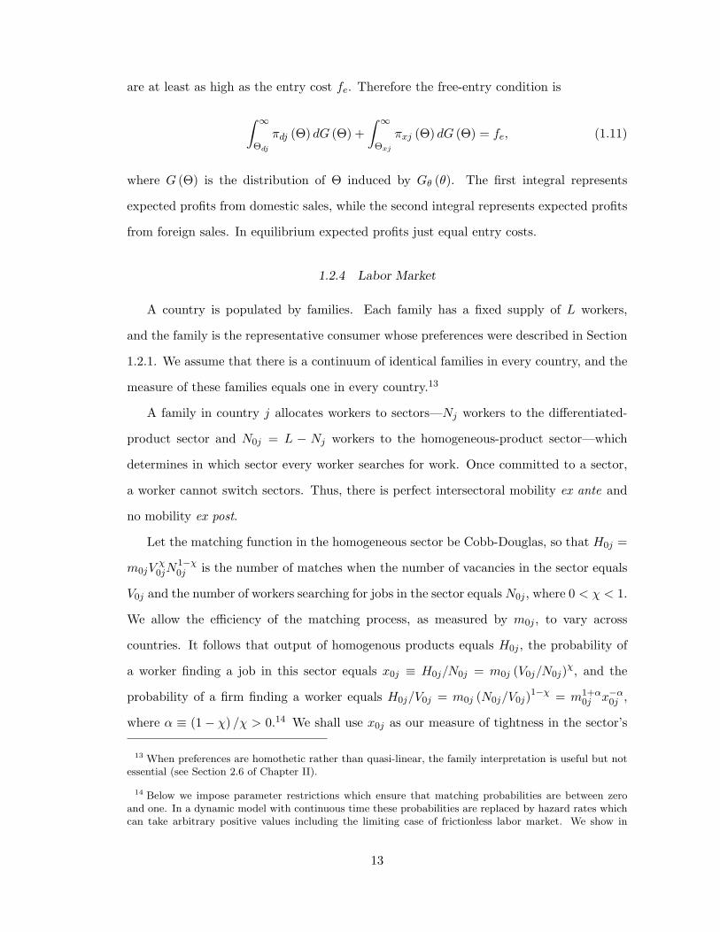
1.2.4 Labor Market

A country is populated by families. Each family has a fixed supply of L workers,

and the family is the representative consumer whose preferences were described in Section

1.2.1. We assume that there is a continuum of identical families in every country, and the

measure of these families equals one in every country.13

A family in country j allocates workers to sectors—Nj workers to the differentiated-

product sector and N0j = L − Nj workers to the homogeneous-product sector—which

determines in which sector every worker searches for work. Once committed to a sector,

a worker cannot switch sectors. Thus, there is perfect intersectoral mobility ex ante and

no mobility ex post.

Let the matching function in the homogeneous sector be Cobb-Douglas, so that H0j =

m0jVχ

0jN1−χ0j is the number of matches when the number of vacancies in the sector equals

V0j and the number of workers searching for jobs in the sector equals N0j , where 0 < χ < 1.

We allow the efficiency of the matching process, as measured by m0j , to vary across

countries. It follows that output of homogenous products equals H0j , the probability of

a worker finding a job in this sector equals x0j ≡ H0j/N0j = m0j (V0j/N0j)χ, and the

probability of a firm finding a worker equals H0j/V0j = m0j (N0j/V0j)1−χ = m1+α

0j x−α0j ,

where α ≡ (1− χ) /χ > 0.14 We shall use x0j as our measure of tightness in the sector’s

13 When preferences are homothetic rather than quasi-linear, the family interpretation is useful but notessential (see Section 2.6 of Chapter II).

14 Below we impose parameter restrictions which ensure that matching probabilities are between zeroand one. In a dynamic model with continuous time these probabilities are replaced by hazard rates whichcan take arbitrary positive values including the limiting case of frictionless labor market. We show in

13

labor market.

Next assume that the cost of posting vacancies equals v0j per worker in country j, mea-

sured in terms of the homogenous good. Then a firm’s entry cost into the industry equals

v0j . After paying this cost the firm is matched with a worker with probability m1+α0j x−α0j

and not matched otherwise. When the firm is matched with a worker they bargain over

the surplus from the relationship, as described in the previous section; the worker gets a

wage w0 = 1/2 and the firm gets a profit π0 = 1/2. Under these circumstances expected

profits equal m1+α0j x−α0j /2 and firms enter up to the point at which these expected profits

cover the entry cost v0j . In other words, in equilibrium tightness in the labor market

equals15

x0j = a−1/α0j , a0j ≡

2v0j

m1+α0j

> 1. (1.12)

The derived parameter a0j summarizes labor market frictions in the homogeneous sector;

it rises with the cost of vacancies and declines with the efficiency of the matching process.

Evidently, tightness in the labor market declines with a0j .

The expected income of a worker searching for a job in the homogenous sector is

ω0j = x0jw0j , which together with (1.12) yields

ω0j =12a−1/α0j . (1.13)

That is, the expected income of this worker rises with the efficacy of matching in the

homogeneous sector and declines with the cost of vacancies. Finally, note that as a result

of free entry of firms, the cost of hiring per worker, b0j ≡ v0jV0j/H0j =(v0j/m

1+α0j

)xα0j ,

equals one half in the homogeneous sector in both countries:

b0j =12a0jx

α0j =

12. (1.14)

Helpman and Itskhoki (2009) that this type of dynamic specification yields steady state outcomes whichare similar to our static specification.

15 We assume that m1+α0j < 2v0j < 1, which ensures that the probability of a worker finding a job and the

probability of a firm finding a worker are both smaller than one. Alternatively, when m1+α0j = 2v0j = 1,

workers and firms are matched with probability one and there is full employment in the homogenous sector,as in Helpman and Itskhoki (2008).

14

We now turn to the differentiated sector. Let Hj be aggregate employment in the

differentiated sector. An individual searching for work in the differentiated-product sector

expects to find a job with probability xj = Hj/Nj , where xj measures the degree of

tightness in the sector’s labor market. Conditional on finding a job an individual expects

to be paid a wage wj = bj (see (1.7)). Therefore the expected income from searching for

a job in the differentiated sector is xjbj .

A family allocates workers to sectors so as to maximize the family’s aggregate income.

A worker allocated to the homogeneous sector earns an expected income of ω0j , given

in (1.13). On the other hand, a worker allocated to the differentiated sector earns an

expected income of xjbj . In an equilibrium with employment in both sectors the two

expected incomes have to be equal. That is, a family chooses 0 < Nj < Lj only if16

xjbj = ω0j . (1.15)

Unemployment in the differentiated sector is an equilibrium outcome when xj < 1. We

provide below parameter restrictions that ensure this condition.

We now interpret the parameter bj of the cost-of-hiring function bjh; this variable is

exogenous to the firm but endogenous to the industry. As in the homogeneous sector,

workers in the differentiated sector are randomly matched with firms. The number of

successful matches is Hj = mjVχj N

1−χj in country j, where Vj is the number of vacancies

and Nj is the number of individuals searching for jobs in this sector. Note that χ is the

same here as in the matching function of the homogenous sector, but mj—which measures

the efficiency of matching—is allowed to differ across countries and sectors. It follows that

when the cost per vacancy is vj in the differentiated sector of country j, then the cost of

hiring is bj = vjVj/Hj per worker, and bj can be related in a simple way to tightness in

the labor market xj :17

bj =12ajx

αj , aj ≡

2vjm1+αj

, (1.16)

16 This is similar to the indifference between staying in the countryside and migrating to the city in theHarris and Todaro (1970) model.

17 See Blanchard and Gali (2008) for a similar specification.

15

where aj is our measure of frictions in the differentiated sector’s labor market, which is

increasing in the cost of vacancies and decreasing in the productivity of matching. Note

the symmetry in the modeling of hiring costs in the homogenous and differentiated sectors

(compare (1.16) with (1.14)).

Next note that (1.12)-(1.16) uniquely determine the hiring cost bj and tightness in the

labor market xj :

xj = x0j

(a0j

aj

) 11+α

=

(1

a1/α0j aj

) 11+α

,

wj = bj = b0j

(aja0j

) 11+α

=12

(aja0j

) 11+α

.

(1.17)

Note that xj < 1 and there is unemployment in the differentiated sector if and only if

a0jaαj > 1, which we assume to be satisfied. It follows from this characterization that

whenever a country has the same labor market frictions in both sectors, so that a0j = aj ,

it has the same labor market tightness in both sectors and the same cost of hiring in both

sectors. Yet while the cost of hiring is independent in this case from the common level

of labor market frictions because b0j = bj = 1/2, tightness in the sectoral labor markets

declines with the level of frictions. This implies that when a0j = aj in both countries no

country has comparative advantage in one of the sectors (see the discussion in the next

section), even when the level of labor market frictions varies across countries. In Helpman

and Itskhoki (2009) we show that similar patterns arise in the steady state of a dynamic

model.

In what follows we assume that aA/a0A > aB/a0B, so that country B has relatively

lower labor market frictions in the differentiated sector. This implies bA > bB, i.e., country

A has a larger hiring cost in the differentiated sector, and xA/x0A < xB/x0B, i.e., the

sectoral labor market tightness is relatively lower in the differentiated sector of country

A. Note, however, that our assumption on relative sectoral labor market frictions has no

implications for whether the labor market is tighter in one sector or the other. When

aj/a0j > 1 in both countries, sectoral tightness is higher in the homogeneous sector in

both countries; when aj/a0j < 1 in both countries, sectoral tightness is higher in the

differentiated sector in both countries; and when aA/a0A > 1 > aB/a0B, sectoral tightness

16

is higher in the homogenous sector in country A and higher in the differentiated sector

in country B. Sectoral labor market frictions can differ due to the fact that it may be

more difficult to match workers with firms in some sectors than in other, and labor market

frictions can differ across countries due to differences in matching efficiency or differences

in costs of posting vacancies.18 We allow these possibilities in order to accommodate

variation in sectoral rates of unemployment, which feature in the data.19

Evidently, the model is bloc recursive, in the sense that the equilibrium wage rate and

tightness in the labor market are uniquely determined by labor market frictions. We show

in Section 1.6 that this property also holds with firing costs and unemployment benefits.

The implication is that labor market frictions determine (bj , xj) in country j, and these

in turn impact other endogenous variables, such as trade, welfare and unemployment.

The sectoral rates of unemployment are 1− x0j in the homogenous sector and 1− xj

in the differentiated sector. As a result, the economy-wide rate of unemployment can be

expressed as

uj =N0j

L(1− x0j) +

Nj

L(1− xj) , (1.18)

which is a weighted average of the sectoral rates of unemployment, where the weights are

the fractions of workers seeking jobs in every sector. It follows that the unemployment

rate can rise either because it rises in one or both sectors or because more individuals

search for work in the sector with a higher rate of unemployment.

1.3 Equilibrium Structure

We focus on equilibria with incomplete specialization, in which every country produces

homogeneous and differentiated products. Conditions for incomplete specialization are

18 In a dynamic model sectors may differ in separation rates, which leads to b0j 6= bj ; see Helpman andItskhoki (2009). Specifically, we show that if the differentiated sector has a higher separation rate it leadsto greater turnover in this sector and a country with more efficient matching technology has a comparativeadvantage in this sector. Furthermore, policy differences can be a source of cross-country variation in labormarket frictions, which we discuss in Section 1.6.

19 To illustrate, the BLS reports that in 2007 Mining had an unemployment rate of 3.4%, Constructionhad 7.4%, and Manufacturing had 4.3% (see http://www.bls.gov/cps/cpsaat26.pdf, accessed on April 25,2008).

17

described in the Appendix, and in our earlier working paper (Helpman and Itskhoki, 2008)

we discuss properties of equilibria with complete specialization. This section is devoted to

a description of equilibria and some of their properties. More substantive results, which

build on this section, are developed and discussed in subsequent sections.

Equations (1.8)-(1.10) yield the following expressions for the domestic market and

export cutoffs:

Θdj =1

φ1φ2fdb

β1−βj Q

β−ζ1−βj ,

Θxj =1

φ1φ2fxb

β1−βj τ

β1−βQ

β−ζ1−β(−j).

(1.19)

Now substitute these expressions into (1.8) and the resulting profit functions into the

free-entry condition (1.11) to obtain

fd

∫ ∞Θdj

(Θ

Θdj− 1)dG(Θ) + fx

∫ ∞Θxj

(Θ

Θxj− 1)dG(Θ) = fe, j = A,B. (1.20)

This form of the free-entry condition generates a curve in (Θdj ,Θxj) space on which every

country’s cutoffs have to be located, because this curve depends only on the common

cost variables and on the common distribution of productivity. Moreover, this curve is

downward-sloping, as depicted by FF in Figure 1.1, and each country has to be located

above the 45o line for the export cutoff to be higher than the domestic cutoff.20

Also note that as the export cutoff goes to infinity, the domestic cutoff approaches the

cutoff of a closed economy, which is represented by Θcd in the figure. It therefore follows

that if the cutoff Θd in the closed economy is larger than Θmin, so is Θd in the open

20 Note, from (1.19), that in a symmetric equilibrium, in which Qj = Q(−j), the export cutoff is higher if

and only if τβ/(1−β)fx > fd, which is the condition required for exporters to be more productive in Melitz(2003). We assume for convenience that this condition is satisfied for all τ ≥ 1 which requires fx > fd.

18

0

xΘ

FdΘ

F

•

o45

•

A

B

cdΘ

BA bb =

•S

•C

Figure 1.1: Cutoffs in a trading equilibrium

economy.21 Finally note that (1.19) yields

Θxj

Θd(−j)=fxτ

β1−β

fd

[bjb(−j)

] β1−β

, j = A,B. (1.21)

Equations (1.20) and (1.21) can be used for solving the four cutoffs as functions of labor

market frictions and cost parameters. As is evident, the cutoffs do not depend on the

levels of the hiring costs bj , only on their relative size. And once the cutoffs have been

solved, they can be substituted into (1.19) to obtain solutions for the real consumption

indexes Qj .

Our primary interest is in the influence of trade and labor market frictions on the

trading countries. We therefore use (1.20) and (1.21) to calculate the impact of these

21 The autarky production cutoff is the solution to

fd

∫ ∞Θcd

(Θ

Θcd

− 1

)dG(Θ) = fe,

which does not depend on labor market frictions. Note also that Θcd > Θmin if and only if

(Θ/Θmin

)>

1 + fe/fd, where Θ is the mean of Θ, which we assume to be satisfied. This results from the fact that theintegral on the left-hand side of the above equation is decreasing in Θc

d and assumes its largest value of(Θ/Θmin

)− 1 when Θc

d = Θmin.

19

variables on the cutoffs, obtaining

Θdj =δxj∆

[−(δx(−j) + δd(−j)

) (bj − b(−j)

)−(δd(−j) − δx(−j)

)τ],

Θxj =δdj∆

[(δx(−j) + δd(−j)

) (bj − b(−j)

)+(δd(−j) − δx(−j)

)τ],

(1.22)

where

δdj =fd

Θdj

∫ ∞Θdj

ΘdG (Θ) , δxj =fx

Θxj

∫ ∞Θxj

ΘdG (Θ) , ∆ =1− ββ

(δdAδdB − δxAδxB) .

Note that δdj/φ2 is average revenue per entering firm from domestic sales in country

j and δxj/φ2 is average revenue per entering firm from export sales.22 Moreover, δdj

equals average gross operating profits (not accounting for fixed costs) per entering firm

from domestic sales and δxj equals average gross operating profits per entering firm from

exporting.

Building on these insights, we prove in the Appendix the following lemmas:

Lemma 1.1. Let bA > bB. Then ΘdA < ΘdB and ΘxA > ΘxB.

Lemma 1.2. An increase in τ raises the export cutoff Θxj and reduces the domestic cutoff

Θdj in both countries.

Lemma 1.3. Let bA > bB. Then QA < QB.

The first lemma shows that in the country with the relatively higher labor market

frictions in the differentiated sector exporting requires higher productivity at the firm

level and that firms with lower productivity at the bottom of the productivity distribution

break even. The former result is quite intuitive; a disadvantage in labor costs needs to be

compensated with a productivity advantage to make exporting profitable. The latter stems

22 To see this, note that profit maximization (1.5) implies πzj(Θ) = φ2Rzj(Θ) − fz for z = d, x, whereRdj(Θ) is revenue from domestic sales and Rxj(Θ) is revenue from foreign sales. Then, from the zero profitconditions (1.9)-(1.10), we have Rzj(Θ) = fz/φ2 · Θ/Θzj . As a result, the average revenues per enteringfirm from domestic sales and exports equal∫ ∞

Θzj

Rzj(Θ)dG(Θ) =fz

φ2Θzj

∫ ∞Θzj

ΘdG(Θ) =δzjφ2, z = d, x.

20

from the fact that in a country with higher bj expected profits from exporting are lower at

the entry stage, which has to be offset by higher expected profits from domestic sales in

order for the free entry condition to be satisfied. This implies that lower-productivity firms

find it profitable to serve the domestic market. The second lemma just restates a well know

result from Melitz (2003) which also holds in our framework: Higher variable trade costs

cut into export profits, enabling only more productive firms to profitably export. Under

the circumstances lower productivity firms need to survive entry in order to be able to

cover the entry cost. The third lemma states that the country with higher relative labor

market frictions in the differentiated sector has lower real consumption of differentiated

products. This stems from the home market effect. Due to the presence of trade costs, a

country suffers a disadvantage in the local supply of differentiated products when its bj is

higher in the differentiated industry.

For our equations to describe an equilibrium with incomplete specialization, it is nec-

essary to ensure positive entry of firms in both countries, i.e., Mj > 0 for j = A,B, where

Mj is the number of firms that enter the differentiated sector in country j. This places

restrictions on the permissible difference across countries in labor market rigidities. To

derive the implications of these restrictions, first recall that Qζj = PjQj is total spending

on differentiated products in country j, and Mjδzj/φ2 is total revenue from domestic sales

when z = d and from foreign sales when z = x. Since aggregate spending has to equal

aggregate revenue in market j, we have

Qζj = Mjδdjφ2

+M(−j)δx(−j)

φ2,

where the first term on the right-hand side is revenues of domestic firms and the second

term is revenues of foreign firms from sales in country j’s market. Having solved for the

cutoffs, which uniquely determine the δzjs, and the real consumption indexes, Qjs, these

equations for j = A,B yield the following solutions for the number of entrants:

Mj =(1− β)φ2

β∆

[δd(−j)Q

ζj − δx(−j)Q

ζ(−j)

]. (1.23)

21

We show in the Appendix that they imply:

Lemma 1.4. In an equilibrium with incomplete specialization: (i) δdj > δxj in both coun-

tries; (ii) if bA > bB, then δdA > δdB and δxA < δxB.

Lemma 1.5. Let bA > bB. Then MA < MB.

Lemma 1.4 is a technical lemma, which describes conditions that hold in an equilib-

rium with incomplete specialization. The economic implication of part (i) is that average

revenue per entering firm from domestic sales exceeds average revenue per entering firm

from export sales in each one of the countries, and the economic implication of part (ii) is

that in country A, which has the relatively higher labor market frictions in the differenti-

ated sector, average revenue per entering firm from domestic sales is higher and average

revenue per entering firm from export sales is lower than in country B. And the last

lemma states that there is less entry of firms in the differentiated product industry in the

country in which labor market frictions are relatively higher in this sector; a result which

is quite intuitive.

Finally, consider the determinants of the number of workers searching for jobs in the

differentiated sector, Nj , and aggregate employment in that sector, Hj . On the one hand,

the wage bill in the differentiated sector, wjHj , equals ω0jNj , because the wage rate is

wj = bj = ω0j/xj (see (1.17)) and xj = Hj/Nj by definition. This implies that aggregate

income equals ω0jL, where income ω0jNj is derived from the differentiated sector and

income ω0jN0 = ω0j (L−Nj) is derived from the homogeneous sector. On the other

hand, the wage bill in the differentiated sector equals the fraction β/ (1 + β) of revenue

(a result from the bargaining game). Therefore

ω0jNj =β

1 + βMj

(δdjφ2

+δxjφ2

), (1.24)

where Mj (δdj + δxj) /φ2 is total revenue of country-j firms from domestic sales and ex-

porting. It follows that, once the cutoffs and the numbers of firms are known, this equation

determines the number of workers searching for jobs in the differentiated-product indus-

22

try.23 Having solved for Nj , aggregate employment in the differentiated sector is

Hj = xjNj . (1.25)

The remaining N0j = L − Nj workers search for jobs in the homogenous-good sector,

with H0j = x0jN0j of them finding employment and generating H0j units of output of

the homogenous good. This completes the description of an equilibrium with incomplete

specialization.

1.4 Trade, Welfare and Productivity

In this section we explore channels through which the two countries are interdependent.

For this purpose we organize the discussion around two main themes: the impact of a

country’s labor market frictions on its trade partner, and the differential effects of trade

impediments on countries with different labor market frictions.

1.4.1 Welfare

We are interested in knowing how labor market rigidities and trade frictions affect

welfare, and in particular their differential impact on the welfare of the two countries.

Since aggregate spending in country j, Ej , equals aggregate income, and aggregate income

equals ω0jL = a−1/α0j L/2 (see (1.13)), the indirect utility function (1.3) implies that welfare

is higher the larger the real consumption index of differentiated products Qj is and the

lower the friction in the homogeneous sector a0j is. We have already shown that Qj is

higher in country B (see Lemma 1.3). It follows that welfare is also higher in B as long

as the labor market friction in its homogenous sector, a0B, is not too high relative to that

in country A, a0A.

Now combine the formulas for change in the cutoffs (1.22) with the log-differential of

23 Recall that ω0j is determined by labor market frictions in the homogeneous sector; see (1.13).

23

the first equation in (1.19) to obtain

β − ζ1− β

Qj =1∆

[−δd(−j) (δxj + δdj) bj + δxj

(δx(−j) + δd(−j)

)b(−j) − δxj

(δd(−j) − δx(−j)

)τ].

(1.26)

This equation has a number of implications. First, it shows that a reduction in a country’s

labor market frictions in the differentiated sector, i.e., a decline in aj which reduces bj

(see (1.17)), raises its real consumption index Qj and therefore its welfare, but it reduces

the trade partner’s welfare. On the other hand, a simultaneous reduction in labor market

frictions in the differentiated sectors of both countries at a common rate aA = aA, which

implies bA = bB, raises everybody’s welfare.24 Second, a reduction in a country’s labor

market frictions at a common rate in both sectors, i.e., a decline in a0j and aj such that

a0j = aj , does not impact its real consumption index Qj nor the real consumption index

of its trade partner Q(−j). As a result, the trade partner’s welfare does not change, yet j’s

welfare rises because expected income of a worker, ω0, rises (see (1.3) and (1.13), and recall

that expenditure equals income, E = ω0jL). Third, in view of Lemma 1.2, a reduction in

trade impediments raises welfare in both countries. We summarize these findings in25

Proposition 1.1. (i) A reduction in labor market frictions in country j’s differentiated

sector raises its welfare and reduces the welfare of its trade partner. (ii) A simultaneous

proportional reduction in labor market frictions in the differentiated sectors of both coun-

tries raises welfare in both of them. (iii) A reduction in labor market frictions in country

j at a common rate in both sectors raises its welfare and does not affect the welfare of

its trade partner. (iv) A reduction of trade impediments raises welfare in both countries

and Qj rises proportionately more in country B, which has relatively lower labor market

frictions in the differentiated sector.

The first part of this proposition is intriguing: it states that a country harms the trade

24 This follows from the fact that −δd(−j) (δxj + δdj) + δxj(δx(−j) + δd(−j)

)= −β∆/ (1− β) < 0.

25 The very last part of the proposition follows from the fact that (1.26) implies

β − ζ1− β

[Qj − Q(−j)

]= − 1

∆

[(δdj + δxj)

(δd(−j) + δx(−j)

) (bj − b(−j)

)+(δd(−j)δxj − δx(−j)δdj

)τ].

Under these circumstances Qj > Q(−j) in response to τ < 0, when bj < b(−j) (by Lemma 1.4) .

24

partner by reducing its labor market frictions. Moreover, this happens despite the fact

that the trade partner (−j) enjoys better terms of trade as a result of improved labor

market conditions in country j, because (−j) pays lower prices for imported varieties

from j and gets access to a larger set of foreign varieties. The reason for this result is

that lower labor market frictions in country j’s differentiated sector act like a productivity

improvements in this country, which makes foreign firms less competitive and therefore

crowds them out from this sector. As a result, fewer foreign firms enter the industry. The

entry of domestic firms does not fully compensate foreign consumers for the exit of foreign

firms due to the home market effect, so that foreign welfare declines, and this negative

welfare effect is larger than the welfare gain from improved terms of trade.26

The last part of this proposition establishes that both countries gain from trade, be-

cause autarky is attained when τ →∞.27 To emphasize this conclusion, we restate it in:

Proposition 1.2. Both countries gain from trade.

This proposition is interesting, because it is well known that gains from trade are not

ensured in economies with nonconvexities and distortions (see Helpman and Krugman,

1985), and in addition to the standard nonconvexities and distortions that exist in models

of monopolistic competition our model contains frictions in labor markets. The intuition is

that every country gains access to a larger variety choice, and in addition, the differentiated

sector—which is too small relative to its first-best size—expands. Together, these effects

of trade opening dominate the welfare outcome.

26 Demidova (2008) studies a full employment model with exogenous differences in productivity distribu-tions across countries, and finds that: (a) productivity improvements in one country hurt its trade partner;and (b) falling trade costs benefit disproportionately the more productive country, and may even hurt theless productive country. Our results on labor market frictions are similar to these (except that in our caseboth countries necessarily gain from falling trade costs), because—not withstanding unemployment—labormarket frictions have analogous effects to productivity. We stress that these effects are analogous but notidentical, because our cross-country differences in relative labor market frictions are not identical to thedifferences in productivity in Demidova’s paper.

27 The following is a direct proof of the gains-from-trade argument: We have seen that the domesticcutoff is higher in every country in the trading equilibrium than in autarky. The first equation in (1.19)then implies that Qj is higher in every country in the trading equilibrium, because this equation also holdsin autarky. In addition, in the earlier working paper Helpman and Itskhoki (2008), we show that bothcountries gain from trade when the difference in labor market institutions is large enough to cause therelatively rigid country to specialize in the production of the homogeneous good. Interestingly, in this casethe gains from trade accrue disproportionately to the relatively rigid country, although its level of welfareis always lower than that of the relatively flexible country.

25

1.4.2 Trade Structure

From Lemma 1.1 we know that the country with lower relative labor market frictions in

the differentiated sector has a lower export cutoff and a higher domestic cutoff; therefore

it also has a larger fraction of exporting firms in the differentiated-product sector. In

addition, we know that exports per entering firm equal δxj/φ2. Therefore exports of

differentiated products from j to (−j) are

Xj = Mjδxjφ2.

Lemma 1.4 states that country B has a larger δxj and Lemma 1.5 states that it has more

firms. Therefore XB > XA, which implies that B exports differentiated products on net.

As a consequence, country A exports homogeneous goods.

As in the standard Helpman-Krugman model of trade in differentiated products, there

is intra-industry trade. We can therefore decompose the volume of trade into intra-

industry and intersectoral trade. Because trade is balanced, the total volume of trade

equals 2XB, the volume of intra-industry trade equals 2XA, and the share of intra-industry

trade equalsXA

XB=δxAMA

δxBMB.

Using this representation we show in the Appendix that the share of intra-industry trade

declines in bA/bB. These results are summarized in

Proposition 1.3. Let bA > bB. Then: (i) A larger fraction of differentiated-sector firms

export in country B. (ii) Country B exports differentiated products on net and imports

homogeneous goods. (iii) The share of intra-industry trade is smaller the larger bA/bB is.

That is, as in Davidson, Martin and Matusz (1999), labor market frictions impact com-

parative advantage, and in our case they also impact the share of intra-industry trade.

In addition, under Pareto-distributed productivity, the model also implies that the vol-

ume of trade is larger the larger is the difference in relative hiring costs across countries,

bA/bB, and the smaller are the trade impediments (see Appendix). These are testable

26

implications of our model.

1.4.3 Productivity

Alternative measures of total factor productivity (TFP) can be used to characterize

the efficiency of production. We choose to focus on one such measure—the employment-

weighted average of firm-level productivity—which is commonly used in the literature.28

In the differentiated sector this measure is

TFP j =Mj

Hj

[∫ ∞Θdj

Θ1−ββ hdj(Θ)dG(Θ) +

∫ ∞Θxj

Θ1−ββ hxj(Θ)dG(Θ)

]. (1.27)

Recall that qzj(Θ) = Θ(1−β)/βhzj(Θ) for z = d, x. Therefore, TFP j equals the output of

differentiated products divided by employment in the differentiated sector.29

Using (1.6) and (1.8)-(1.10), we can express (1.27) as

TFP j =δdjϕdj + δxjϕxj

δdj + δxj= $djϕdj +$xjϕxj , (1.28)

where $dj = δdj/(δdj + δxj) is the share of domestic sales in revenue and $xj is the share

of exports, i.e., $xj = 1−$dj , j = A,B. Moreover,

ϕzj ≡ ϕ(Θzj) =

∫∞Θzj

Θ1/βdG(Θ)∫∞Θzj

ΘdG(Θ), z = d, x,

where ϕdj represents the average productivity of firms that serve the home market and ϕxj

represents the average productivity of exporting firms. It follows that aggregate productiv-

ity equals the weighted average of the productivity of firms that serve the domestic market

28 This corresponds to the measure analyzed by Melitz (2003) in the appendix. Note that Melitz usesrevenue to weight firm productivity levels. However, in equilibrium, revenue is proportional to employment,in which case his and our productivity indexes are the same.

29 An alternative, and potentially more desirable, measure of productivity, would divide output by thenumber of workers searching for jobs in the differentiated-product sector, Nj . This measure is alwayssmaller than TFPj by the factor xj . It follows that labor market liberalization has an additional positiveeffect on this measure of productivity as compared to the measure used in the main text. Also note thatTFPj measures productivity in the differentiated-product sector only, rather than in the entire economy,and productivity in the homogeneous-product sector is constant given a0j . We discuss in the Appendix aproductivity measure that accounts for the compositional effects across sectors.

27

and the productivity of firms that export, with the revenue shares serving as weights. We

show in the Appendix that ϕ(·) is an increasing function. Therefore average productivity

is higher among exporters, i.e., ϕxj > ϕdj .

Expression (1.28) implies that the cutoffs Θdj ,Θxj uniquely determine the TFP js,

because $zj and ϕzj depend only on the cutoffs. Moreover, since the two cutoffs are linked

by the free-entry condition (1.20), TFP j can be expressed as a function of the domestic

cutoff Θdj . This implies that in a closed economy TFP j is not responsive to changes in

labor market frictions, because Θcd is uniquely determined by the fixed costs of entry and

production and the ex ante productivity distribution.

Productivity TFP j is higher in the trade equilibrium than in autarky, however, because

ϕ(Θxj) > ϕ(Θdj) > ϕ(Θcd), and in autarky $c

x = 0. That is, the average productivity of

exporters and nonexporters alike is higher in the trade equilibrium than is the average

productivity of firms in autarky. In addition, trade reallocates revenue to the exporting

firms, which are on average more productive. For both these reasons trade raises TFP j .

We summarize these results in

Proposition 1.4. (i) In the closed economy, TFPj does not depend on labor market

frictions. (ii) TFPj is higher in any trade equilibrium than in autarky.

Next recall that in an open economy a reduction of trade costs raises the domestic

cutoff and reduces the export cutoff. In addition, a reduction in country j’s labor market

frictions in the differentiated sector raises Θdj and Θx(−j) and reduces Θd(−j) and Θxj .

Finally, a simultaneous and proportional decline in both countries’ labor market frictions

in the differentiated sector (i.e., bA = bB < 0) leaves all these cutoffs unchanged (see

(1.22)).

How do changes in labor market frictions impact productivity? In the case in which

both countries’ labor market frictions decline by the same factor of proportionality, the

answer is simple: the TFP js do not change. As long as productivity is measured with

regard to the number of employed workers rather than the number of workers searching for

jobs, measured sectoral productivity levels are not sensitive to the absolute levels of bjs;

only the relative levels matter. This result points to a shortcoming of this TFP measure.

28

We nevertheless continue the analysis with this measure, because it is commonly used in

the literature.

A shock that raises the domestic cutoff Θdj and reduces the export cutoff Θxj affects

TFP j through three channels. First, the reallocation of revenue from firms that serve the

home market to exporters raises the weight on the productivity of exporters, $xj , which

raises in turn TFP j . Second, some least-efficient firms exit the industry, thereby raising

the average productivity of firms that sell only in the home market, ϕdj , which raises

TFP j . Finally, some firms with productivity below Θxj begin to export, thereby reducing

the average productivity of exporters, ϕxj , which reduces TFP j .30

The presence of the third effect, which goes against the first two, does not enable us

to sign the impact of single-country reductions of labor market frictions on productivity;

in general, productivity may increase or decrease. The sharp result for the comparison

of autarky to trade derives from the fact that, in a move from autarky to trade, the

third effect is nil. In the Appendix, we provide sufficient conditions for productivity to

be monotonically rising with Θdj , and therefore declining with bj and τ and rising with

b(−j). In this section, however, we limit our discussion to the case of Pareto-distributed

productivity draws, which yields sharp predictions.

Under the assumption of Pareto-distributed productivity, that is, G (Θ) = 1−(Θmin/Θ)k

for Θ ≥ Θmin, (1.28) results in (see Appendix):

TFP j =δdj(ϕxj − ϕdj

)(1 + k − 1/β

)δdjϕdj + δxjϕxj

Θdj , (1.29)

where k > 1/β is required for TFP j to be finite, and we therefore assume that it holds,

and an increase in Θdj is accompanied by a corresponding decrease in Θxj in order to

satisfy the free-entry condition. As a result, TFP j is higher the higher Θdj is (and the

lower Θxj is). It follows that productivity is higher in country B, and a reduction in

a country’s labor market frictions in the differentiated sector raises its productivity and

reduces the productivity of its trade partner. An implication of this result is that the

30 Formally, this decomposition can be represented as TFPj = $xj(ϕxj − ϕdj) + (1−$xj)ϕdj +$xjϕxjwith $xj > 0, ϕdj > 0 and ϕxj < 0.

29

gap in productivity between countries B and A is increasing in bA/bB and therefore in

aA/aB, their relative labor market frictions in the differentiated sector. These results are

summarized in

Proposition 1.5. Let bA > bB and let Θ be Pareto-distributed with shape parameter

k > 1/β. Then: (i) TFPj is higher in B; (ii) a decline in aj raises TFPj and reduces

TFP(−j); (iii) a reduction of trade costs τ raises TFPj in both countries.

In other words, total factor productivity is higher in the country with relatively lower

labor market frictions in the differentiated sector, and while a reduction of labor market

frictions in this sector in any country raises its own total factor productivity, this hurts

the total factor productivity of the country’s trade partner.

1.5 Unemployment

Before discussing the variation of unemployment across countries with different labor

market frictions in Section 1.5.2, we first examine the determinants of unemployment in

a world of symmetric countries.

1.5.1 Symmetric Countries

We study in this section countries with a0A = a0B = a0 and aA = aB = a, so

that bA = bB = b, in order to understand how changes in the common levels of labor

market frictions and the common level of variable trade cost affect unemployment. In

such equilibria, the cutoffs Θd and Θx, the consumption index Q, the number of entrants

M , the number of individuals searching for jobs in the differentiated-product sector N ,

the number of workers employed in that sector H, and the rate of unemployment u are

the same in both countries. We therefore drop the country index j for convenience. From

Section 1.3 we know that two symmetric economies are at the same point on the FF curve

in Figure 1.1 (point S), the location of this point is invariant to the common level of labor

market frictions, and this point is higher the larger τ is. Moreover, (1.26) implies that

Q is lower the higher are either b or τ . When b is higher as a result of higher frictions

30

in the labor market of the differentiated sector, welfare is lower because Q is lower while

aggregate income E = ω0L is not affected (recall that welfare is given by (1.3)).

Figure 1.2: Unemployment in a world of symmetric countries

In order to assess the impact of labor market rigidities on unemployment, we need to

know their quantitative impact on Q. For this reason we use (1.26) to obtain

Q = − β

β − ζ

(b+

δxδd + δx

τ

).

Next combine (1.23) and (1.24) to obtain ω0N = βQζ/ (1 + β), which together with the

previous equation yields

N = − βζ

β − ζ

(b+

δxδd + δx

τ

)under the assumption that changes in b are driven by changes in a, our measure of labor

market frictions in the differentiated sector. In other words, in this analysis we keep

constant the level of labor market frictions in the homogeneous sector, a0 (below we

discuss the case of simultaneous reductions in labor market frictions in both sectors).

31

Finally, from (1.17) and (1.18) together with the formula for N we obtain31

sign u = sign[

1− (2b− 1)βζ

β − ζ

]b− (2b− 1)

βζ

β − ζδx

δd + δxτ

.

It is evident from this formula that lower frictions in the differentiated sector’s labor

market (lower b) reduce unemployment if and only if

2b =(a

a0

) 11+α

< 1 +β − ζβζ

,

i.e., if and only if labor market frictions are low in this sector to begin with. This condition

is always satisfied when labor market frictions are higher in the homogeneous sector, i.e.

a0 > a. If labor market frictions in the differentiated sector are high, however, and the

above inequality is reversed, then a reduction in a—and hence in b—may raise the rate of

unemployment. In fact, the relationship between b and the rate of unemployment has an

inverted U shape as depicted in Figure 1.2.

To understand this result, note that changes in a impact unemployment through two

channels: the rate of unemployment in the differentiated sector 1− x, and the fraction of

individuals searching for jobs in this sectorN/L. Reductions in these labor market frictions

raise x and thereby reduce the sectoral rate of unemployment. On the other hand, such

reductions attract more workers to the differentiated-product sector and thereby reduce

the rate of unemployment if and only if the sectoral rate of unemployment is higher in

the homogeneous sector (i.e., x < x0). When a0 > a the sectoral rate of unemployment

is higher in the homogenous sector and both channels lead to a reduction in the rate

of unemployment. On the other hand, when a > a0, the two channels conflict, and the

latter, i.e., the reallocation of labor toward the differentiated sector, dominates when labor

31 In this derivation we use bx = b0x0 = ω0, where ω0 is given in (1.13) and it does not vary with a, themeasure of labor market frictions in the differentiated sector. Therefore, b = −x. Also note that x0 = 0since b0 ≡ 1/2. We have

uLu = dN(x0 − x)−Ndx = xN[(x0

x− 1)N + b

].

From (1.17), x0/x =(a/a0

)1/(1+α)= 2b. Finally, combining these results with the expression for N , we

obtain the result in the text.

32

market frictions are high.32

Next consider a proportional reduction in both sectors’ labor market frictions, i.e.,

a0 = a < 0. This has no effect on the search cost b and does not impact the real

consumption index Q (see (1.17) and (1.26)). However, it reduces expected income ω0:

from (1.13), ω0 = −a/α. It therefore follows from ω0N = βQζ/ (1 + β) that N = a/α,

and it follows from (1.17) that x = x0 = −a/α. Using these expressions, and N0 +

N = L, the unemployment formula (1.18) implies that sign u = sign a. In other

words, a reduction of labor market frictions at a common rate in both sectors reduces the

rate of unemployment. Note that this sort of change in labor market frictions impacts

unemployment through two channels, which may operate in opposite directions. On one

hand, it raises tightness in each sector’s labor market, thereby reducing both sectoral

rates of unemployment. On the other hand, it leads to a reallocation of workers from the

differentiated to the homogeneous sector. If the sectoral rate of unemployment is higher in

the differentiated sector, this reduces the rate of unemployment. But if the sectoral rate of

unemployment is lower in the differentiated sector, this raises the rate of unemployment.

Nevertheless, the composition effect is dominated by the sectoral effects.33

Finally, consider changes in trade impediments. As the formula for the sign of changes

in the rate of unemployment shows, a lower trade cost τ raises the rate of unemployment

if and only if b > 1/2 (i.e., a > a0).34 In this case the impact on unemployment operates

only through the reallocation of labor across sectors, because sectoral unemployment rates

do not change. In particular, more workers search for jobs in the differentiated sector when

τ declines, and therefore aggregate unemployment rises when the differentiated sector has

higher sectoral unemployment and aggregate unemployment falls when the differentiated

sector has lower sectoral unemployment. Since the lowering of trade costs raises welfare,

32 It can also be shown that in the symmetric case lower a lead to increased entry of firms M , an increasein N proportionately to M , and a more than proportional increase in employment H.

33 From (1.18) and N0 + N = L we obtain uLu = −N0x0x0 −Nxx + (x0 − x)NN , where the first twoexpressions on the right-hand sided represent the sectoral effects and the third represents the compositioneffect. Since x = x0 = −N = −a/α, the sectoral effects dominate.

34 The effect of a reduction in trade costs on unemployment is larger the larger is the share of trade inthe sector’s revenue, i.e., the larger is δxj/ (δdj + δxj). When the economies are nearly closed, this effect isvery small.

33

this means that welfare and unemployment may respond in opposite directions to changes

in trade costs.

We summarize the main findings of this section in

Proposition 1.6. In a symmetric world economy: (i) reductions in labor market frictions

in the differentiated sectors at the same rate in both countries reduce aggregate unemploy-

ment if and only if a < a0 · [1 + (β − ζ) /βζ]1+α; (ii) reductions in labor market frictions

at a common rate in both sectors and both countries reduce aggregate unemployment; (iii)

reductions in trade impediments raise aggregate unemployment if and only if a > a0.

An intriguing result is that lower trade barriers may raise unemployment. Lower trade

costs make exporting more profitable in the differentiated-product sector. Moreover, the

tightness in its labor market is not affected by falling trade costs. This increases demand

for labor in the differentiated sector and leads to reallocation of workers towards this

sector. Under these circumstances, the sectoral unemployment rates remain the same,

but the aggregate unemployment rate may increase or decrease due to the compositional

effect across sectors.35 The direction of this effect depends on whether the differentiated

sector has a higher or lower unemployment rate.

Also note that unemployment can increase or decrease when welfare rises. That is,

depending on the nature of the disturbance and the initial labor market frictions, unem-

ployment and welfare can move in the same or in opposite directions. For this reason

changes in unemployment do not necessarily reflect changes in welfare. This results from

the standard property of search and matching models, in which unemployment is a pro-

ductive activity which leads to creation of productive matches. Under these circumstances

an expansion of the high-wage\high-unemployment sector results in higher unemployment,

but may also raise welfare.

35 See Felbermayr, Prat and Schmerer (2008) for a one-sector search model in which trade causes anincrease in sectoral labor market tightness by reducing the real cost of vacancies, but naturally has nocompositional effect.

34

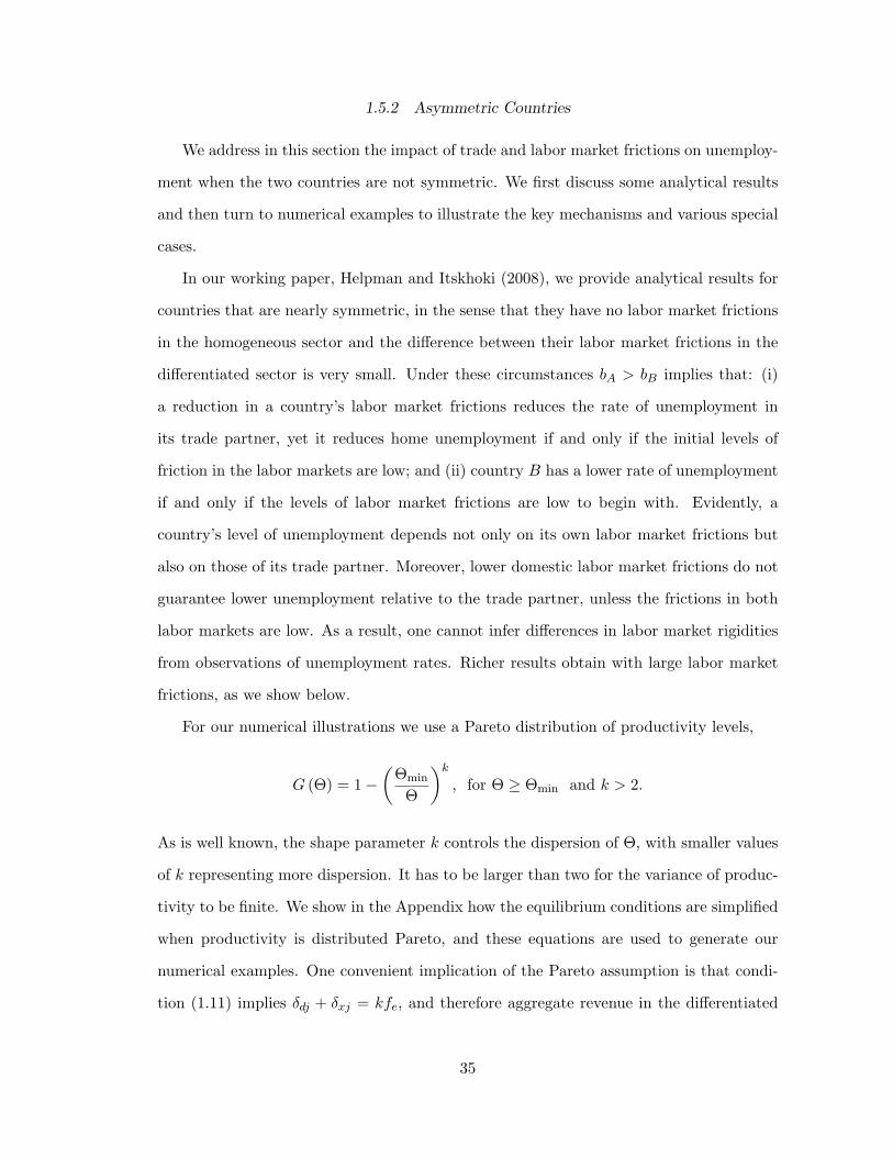
1.5.2 Asymmetric Countries

We address in this section the impact of trade and labor market frictions on unemploy-

ment when the two countries are not symmetric. We first discuss some analytical results

and then turn to numerical examples to illustrate the key mechanisms and various special

cases.

In our working paper, Helpman and Itskhoki (2008), we provide analytical results for

countries that are nearly symmetric, in the sense that they have no labor market frictions

in the homogeneous sector and the difference between their labor market frictions in the

differentiated sector is very small. Under these circumstances bA > bB implies that: (i)

a reduction in a country’s labor market frictions reduces the rate of unemployment in

its trade partner, yet it reduces home unemployment if and only if the initial levels of

friction in the labor markets are low; and (ii) country B has a lower rate of unemployment

if and only if the levels of labor market frictions are low to begin with. Evidently, a

country’s level of unemployment depends not only on its own labor market frictions but

also on those of its trade partner. Moreover, lower domestic labor market frictions do not

guarantee lower unemployment relative to the trade partner, unless the frictions in both

labor markets are low. As a result, one cannot infer differences in labor market rigidities

from observations of unemployment rates. Richer results obtain with large labor market

frictions, as we show below.

For our numerical illustrations we use a Pareto distribution of productivity levels,

G (Θ) = 1−(

Θmin

Θ

)k, for Θ ≥ Θmin and k > 2.

As is well known, the shape parameter k controls the dispersion of Θ, with smaller values

of k representing more dispersion. It has to be larger than two for the variance of produc-

tivity to be finite. We show in the Appendix how the equilibrium conditions are simplified

when productivity is distributed Pareto, and these equations are used to generate our

numerical examples. One convenient implication of the Pareto assumption is that condi-

tion (1.11) implies δdj + δxj = kfe, and therefore aggregate revenue in the differentiated

35

sector is independent of labor market frictions and is the same in both countries. For the

simulations we also assume that a0A = a0B = a0, so that labor market frictions in the

homogenous sector are the same in both countries, as a result of which expected income

of workers, ω0j , is also the same in both countries, i.e., ω0A = ω0B = ω0. In addition, we

assume that aA > aB > a0, so that labor market frictions are larger in the differentiated

sectors of both countries than in their homogeneous sectors, and particularly so in country

A. This implies bA > bB > 1/2.

Combining (1.23) and (1.24), we obtain the following expression for global revenues

generated in the differentiated sector:

QζA +QζB =1φ2

[MA(δdA + δxA) +MB(δdB + δxB)

]=

1 + β

βω0(NA +NB).

Therefore, whenever QζA +QζB rises, the world-wide allocation of workers to the differen-

tiated sector, NA +NB, must also increase.36 Next note that Proposition 1.1 establishes

that a reduction in trade costs raises Qj in both countries. Therefore, the above discussion

implies that a reduction in trade costs increases NA +NB. In the Appendix we also show

that NA/NB declines with reductions in τ when bA > bB. This then implies that NB, the

number of job-seekers in the differentiated sector of country B, necessarily increases. Since

a fall in τ does not affect sectoral labor market tightness, we conclude that a reduction in

trade costs increases unemployment in country B, which has lower labor market frictions

in the differentiated sector. The effect on NA and hence on the unemployment rate in

country A is ambiguous, as we illustrate below.

The intuition behind this result is the following. Lower trade impediments increase

the global size of the differentiated sector, which features increasing returns to scale and

love of variety. As a result, the country with a more flexible labor market, which has

a competitive edge in this sector, becomes more specialized in differentiated products.

36 Note that this result does not rely on the Pareto assumption. Under the Pareto assumption, however,we additionally have QζA + QζB = kfe(MA + MB)/φ2, so that the total number of entrants into thedifferentiated sector must also increase. Moreover, in the Appendix we show that in this case ω0Nj/Mj =βkfe/(1− β). That is, the number of workers searching for jobs in the differentiated sector relative to thenumber of firms depends on expected income ω0, but does not depend on the trade cost or labor marketfrictions in the differentiated sector.

36

That is, the number of entering firms, employment, and the number of job-seekers in the

differentiated sector, all increase in country B. This compositional shift leads to a higher

rate of unemployment in this country, because the sectoral rate of unemployment is higher

in the differentiated sector. Finally, the reallocation of labor in country A may shift in

either direction, depending on how strong the comparative advantage is (see below).

A

0.5 0.55 0.6 0.65 0.70

0.01

0.02

0.03

0.04

0.05

0.06

0.07

0.08

0.09

0.1

Bu

Au

BbAb'b ''b

Figure 1.3: Unemployment as a function of bA when bB is low (bB = 0.55)

Figure 1.3 depicts the response of unemployment rates to variation in country A’s labor

market frictions aA, which changes monotonically bA; the rising broken-line curve repre-

sents country B and the hump-shaped solid-line curve represents country A.37 Country B

has bB = 0.55 > 1/2, and therefore the two countries have the same rate of unemployment

when bA = 0.55. As bA rises, country A becomes more rigid. This raises initially the rate

of unemployment in both countries, but B’s rate of unemployment remains lower for a

while. At some point, however, the rate of unemployment reaches a peak in country A,

and it falls for further increases in bA. As a result, the two rates of unemployment become

equal again, after which further increases in rigidity in country A raise the rate of unem-

ployment in country B and reduce it in country A, so that the rate of unemployment is

higher in country B thereafter. The mechanism that operates here is that once the labor

market frictions become high enough in country A, the contraction of the differentiated-

37 In Figures 1.3-1.4 we use the following parameters: m0 = 2v0 = 1, fx = 3, fd = 1, fe = 0.5, k = 2.5,β = 0.75, ζ = 0.5, L = 0.1 and τ = 1.1 when it is held constant.

37

product sector leads to overall lower unemployment in A despite the fact that its sectoral

unemployment rate is high. When bA is very high the sectoral unemployment rate is very

high, but no individuals search for jobs in this sector, as a result of which there is no

unemployment at all. This explains the hump in A’s curve. Note that in the range in

which the rate of unemployment falls in country A the rate of unemployment keeps rising

in country B. The reason is that there is no change in market tightness in country B

and its differentiated-product sector becomes more competitive the more rigid the labor

market becomes in A. As a result the differentiated sector attracts more and more workers

in country B, which raises its rate of unemployment. The monotonic impact of country

A’s labor market rigidities on the unemployment rate in B holds globally, and not only

around the symmetric equilibrium.38

0.5 0.55 0.6 0.65 0.7 0.75 0.80

0.02

0.04

0.06

0.08

0.1

0.12

0.14

0.16

0.18

0.2

Bu

BbAb'b

Au

ob

Figure 1.4: Unemployment as a function of bA when bB is high (bB = 0.65)

Figure 1.4 is similar to Figure 1.3, except that now the level of labor market frictions

in country B is higher, i.e., bB = 0.65 > 1/2, and therefore the two curves intersect at

bA = 0.65. Moreover, starting with a symmetric world that has these higher labor market

rigidities, increases in bA always raise unemployment in B and reduce unemployment in A.

As a result, country A has lower unemployment when bA > bB and higher unemployment

when bA < bB. That is, in this case a more rigid country always has a lower unemployment

38 In Figures 1.3-1.4, country A specializes in the homogeneous good when bA ≥ b′; in Figure 1.4,country B specializes in the homogeneous good when bA ≤ bo; in Figure 1.3 country B specializes in thedifferentiated good for bA ≥ b′′.

38

rate when it specializes (incompletely) in the low-unemployment sector.

A comparison between Figures 1.3 and 1.4 demonstrates the importance of the overall

level of labor market rigidities for unemployment outcomes. When labor market frictions

are high, a relatively more flexible country always has a higher rate of unemployment.

Moreover, the rates of unemployment in the two countries move in opposite directions

as labor market frictions change in either one of the countries. In contrast, when labor

market rigidities are low and the difference in labor market frictions across countries is

not large, the rate of unemployment is lower in a more flexible country and the rates of

unemployment in both countries co-move in response to changes in labor market frictions.

1 1.1 1.2 1.3 1.4 1.5 1.6 1.7 1.8 1.9 20.03

0.04

0.05

0.06

0.07

0.08

0.09

0.10

0.11

0.12

Bu

τ

Au

Figure 1.5: Unemployment as a function of τ when bA and bB are low (bA = 0.6 andbB = 0.56)

The next three figures depict variations in unemployment in response to trade frictions,

in the form of variable trade costs τ : Figure 1.5 for the case of low frictions in labor

markets, Figure 1.6 for the case in which frictions are low in country B but high in A, and

Figure 1.7 for the case in which frictions are high in both countries.39 In all three cases

unemployment rises in B and falls in A when trade frictions decline.40 Nevertheless, the

39 In Figures 1.5-1.7 we use the following parameters: m0 = 2v0 = 1, fx = 5, fd = 1, fe = 0.5, k = 2.5,β = 0.75, ζ = 0.5, and L = 0.1.

40 This pattern is not general. As we know, in the symmetric case lower trade impediments raise un-employment in both countries, which is also the case when countries are nearly symmetric. We can alsoprovide examples in which the rigid country has a hump in its rate of unemployment as trade frictionsvary.

39

1 1.1 1.2 1.3 1.4 1.5 1.6 1.7 1.8 1.9 20.03

0.04

0.05

0.06

0.07

0.08

0.09

0.1

0.11

0.12

Bu

τ

Au

Figure 1.6: Unemployment as a function of τ when bA is high and bB is low (bA = 0.68and bB = 0.56)

τ1 1.1 1.2 1.3 1.4 1.5 1.6 1.7 1.8 1.9 2

0.03

0.04

0.05

0.06

0.07

0.08

0.09

0.1

0.11

0.12

Bu

Au

Figure 1.7: Unemployment as a function of τ when bA and bB are high (bA = 0.95 andbB = 0.8)

rate of unemployment is not necessarily higher in A. In particular, unemployment is always

higher in A when frictions in labor markets are low in both countries, yet unemployment is

always higher in B when frictions in labor markets are high in both countries. In between,

when labor market frictions are low in B and high in A, the relative rate of unemployment

depends on trade impediments; it is lower in A when the trade frictions are low and lower

in B when the trade frictions are high. This shows that labor market frictions interact

with trade impediments in shaping unemployment.

40

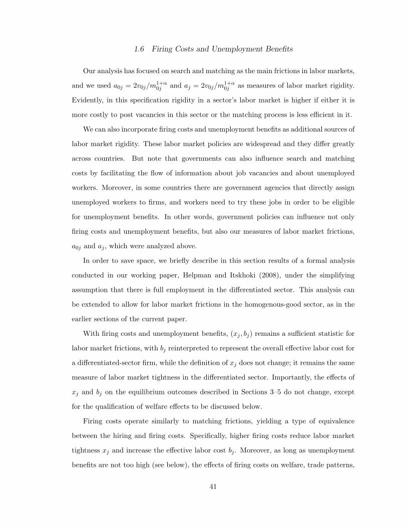
1.6 Firing Costs and Unemployment Benefits

Our analysis has focused on search and matching as the main frictions in labor markets,

and we used a0j = 2v0j/m1+α0j and aj = 2v0j/m

1+α0j as measures of labor market rigidity.

Evidently, in this specification rigidity in a sector’s labor market is higher if either it is

more costly to post vacancies in this sector or the matching process is less efficient in it.

We can also incorporate firing costs and unemployment benefits as additional sources of

labor market rigidity. These labor market policies are widespread and they differ greatly

across countries. But note that governments can also influence search and matching

costs by facilitating the flow of information about job vacancies and about unemployed

workers. Moreover, in some countries there are government agencies that directly assign

unemployed workers to firms, and workers need to try these jobs in order to be eligible

for unemployment benefits. In other words, government policies can influence not only

firing costs and unemployment benefits, but also our measures of labor market frictions,

a0j and aj , which were analyzed above.

In order to save space, we briefly describe in this section results of a formal analysis

conducted in our working paper, Helpman and Itskhoki (2008), under the simplifying

assumption that there is full employment in the differentiated sector. This analysis can

be extended to allow for labor market frictions in the homogenous-good sector, as in the

earlier sections of the current paper.

With firing costs and unemployment benefits, (xj , bj) remains a sufficient statistic for

labor market frictions, with bj reinterpreted to represent the overall effective labor cost for

a differentiated-sector firm, while the definition of xj does not change; it remains the same

measure of labor market tightness in the differentiated sector. Importantly, the effects of

xj and bj on the equilibrium outcomes described in Sections 3–5 do not change, except

for the qualification of welfare effects to be discussed below.

Firing costs operate similarly to matching frictions, yielding a type of equivalence

between the hiring and firing costs. Specifically, higher firing costs reduce labor market

tightness xj and increase the effective labor cost bj . Moreover, as long as unemployment

benefits are not too high (see below), the effects of firing costs on welfare, trade patterns,

41

productivity and unemployment in trading economies, are the same as those of matching

frictions. That is, all the earlier results of this paper extend to the case in which there are

positive firing costs in addition to matching frictions.

Higher unemployment benefits always reduce equilibrium labor market tightness xj ,

but they may increase or decrease the effective labor cost bj . The intuition for this

result is that unemployment benefits provide unemployment insurance to the workers on

the one hand and a better outside option in the wage bargaining game on the other.

Because higher unemployment benefits provide better unemployment insurance, workers

are willing to search for jobs in a less tight labor market, with a higher sectoral rate of

unemployment. This effect reduces the cost of hiring for firms. On the other side the better

outside option of workers at the wage bargaining stage improves their bargaining position

and increases the effective cost of labor to firms. Either one of these effects can dominate.

Therefore bj may rise or decline in response to higher unemployment benefits. When bj

decreases, it leads to an expansion of the differentiated sector, which raises welfare. But

because unemployment benefits need to be financed by (lump-sum) taxes, the additional

taxes required to finance higher unemployment benefits reduce disposable income and hurt

welfare. Therefore on net welfare may rise or decline, but it definitely rises in response

to a small rise in unemployment benefits that reduces bj when the initial level of these

benefits is small.41

We also show that firing costs and unemployment benefits not withstanding, interna-

tional trade may raise unemployment in both countries. The reason is that trade attracts

more workers to the differentiated sector without affecting sectoral labor market tightness.

Therefore, when this sector has the lower labor market tightness, trade increases aggregate

unemployment.

41 Severance pay affects labor costs similarly to unemployment benefits, except that it has no impact ondisposable income.

42

1.7 Concluding Comments

We have studied the interdependence of countries that trade homogeneous and dif-

ferentiated products, and whose labor markets are characterized by search and matching

frictions. Variation in labor market frictions and the interactions between trade impedi-

ments and labor market rigidities generate rich patterns of unemployment. For example,

lower frictions in a country’s labor markets do not ensure lower unemployment, and un-

employment and welfare can both rise in response to a policy change.

Contrary to the complex patterns regarding unemployment, the model yields sharp pre-

dictions about welfare. In particular, both countries gain from trade. Moreover, changes

in one country’s labor market frictions can differentially impact welfare of the trade part-

ners. For example, reducing a country’s frictions in the labor market of the differentiated

sector raises competitiveness of its firms. This improves the foreign country’s terms of

trade, but also crowds out foreign firms from the differentiated-product sector. As a re-

sult, welfare rises at home and declines abroad, because the terms-of-trade improvement

in the foreign country is outweighed by the decline in the competitiveness of its firms.

Nevertheless, a common reduction in labor market frictions in the differentiated sectors

raises welfare in both countries. These results contrast with the implications of models

of pure comparative advantage, in which movements in the terms of trade dominate the

outcomes.42

We also show that labor market frictions confer comparative advantage, and that

differences in these labor market characteristics shape trade flows. In particular, the

country with relatively lower labor market frictions in the differentiated sector exports

differentiated products on net and imports homogeneous goods. Moreover, the larger the

difference in these relative frictions, the lower is the share of intra-industry trade. These

are testable implications about trade flows and international patterns of specialization.

42 See, for example, Brugemann (2003) and Alessandria and Delacroix (2008). The former examines thesupport for labor market rigidities in a Ricardian model in which the choice of regime impacts comparativeadvantage. The latter analyzes a two-country model with two goods, in which every country specializes ina different product and governments impose firing taxes. The authors find that a coordinated eliminationof these taxes yields welfare gains for both counties, yet no country on its own has an incentive to do it.

43

In addition, we show that trade raises total factor productivity in the differentiated-

product sectors of both countries, while productivity does not change in the homogeneous

sector. And productivity is higher in the country with relatively lower labor market

frictions in the differentiated sector.

An important conclusion from our analysis is that simple one-sector macro models

that ignore compositional effects may be inadequate for assessing labor market frictions,

and especially so in a world of integrated economies. Moreover, a focus on terms-of-trade

as the major channel of the international transmission of shocks misses the impact of

competitiveness, which can dominate economic outcomes.

44

2. INEQUALITY AND UNEMPLOYMENT IN A GLOBAL ECONOMY

(with Elhanan Helpman and Stephen J. Redding)

2.1 Introduction

Two core issues in international trade are the allocation of resources across economic

activities and the distribution of incomes across factors of production. Recent research

has emphasized the allocation of resources across heterogeneous firms, but has largely

concentrated on heterogeneity in the product market (productivity and size) rather than

the labor market (workforce composition and wages). Developing trade models that incor-

porate both product and labor market heterogeneity is therefore important for explaining

firm data and understanding the consequences of trade liberalization. To the extent that

wages vary across firms within sectors, reallocations of resources across firms provide an

additional channel for international trade to influence income distribution.

In this paper, we develop a new framework for examining the distributional conse-

quences of trade that incorporates this channel and captures three plausible features of

product and labor markets. First, there is heterogeneity in firm productivity, which gen-

erates differences in firm profitability. Second, search and matching frictions in the labor

market imply that workers outside a firm are imperfect substitutes for those inside the

firm, which gives rise to multilateral bargaining between each firm and its workers. Third,

workers are heterogeneous in terms of match-specific ability, which can be imperfectly

observed by firms. Together these three components of the model generate variation in

wages across firms within industries and imply that trade liberalization affects income

distribution.

In the closed economy, we derive a sufficient statistic for wage inequality, which deter-

mines all scale-invariant measures of wage inequality, such as the Coefficient of Variation,

Gini Coefficient and Theil Index. This sufficient statistic depends on the dispersion param-

eters for worker ability and firm productivity as well as other product and labor market

parameters that influence workforce composition. Greater dispersion of worker ability has

ambiguous effects on wage inequality, because it affects both relative wages and employ-

ment levels across firms. In contrast, greater dispersion of firm productivity raises wage

inequality, because more productive firms pay higher wages. This close relationship be-

tween wage and productivity dispersion within industries receives empirical support from

studies using micro data, including Davis and Haltiwanger (1991) and Faggio, Silvanes

and Van Reenen (2007).

In the open economy, only the most productive firms export; firms of intermediate

productivity serve only the domestic market; and the least productive firms exit without

producing because they cannot cover fixed production costs. Exporting firms have higher

revenue than non-exporting firms, screen workers more intensively, employ workforces of

higher average ability, and pay higher wages. The model therefore is consistent with

empirical findings that exporters pay higher wages than non-exporters (see for example

Bernard and Jensen, 1997) and that a substantial component of this wage difference is

explained by workforce composition (see for example Kaplan and Verhoogen, 2006, Schank,

Schnabel and Wagner, 2007, and Munch and Skaksen, 2008).

The open economy wage distribution is a mixture of the wage distributions for em-

ployees of domestic and exporting firms, with exporters paying higher wages than non-

exporters. Therefore the open economy wage distribution depends on the fraction of

exporters and the exporter wage premium, as well as on the sufficient statistic for wage in-

equality from the closed economy. Opening closed economies to trade increases wages and

employment at high-productivity exporters relative to low-productivity domestic firms.

As a result the opening of trade raises wage inequality for any measure of wage inequality

that respects second-order stochastic dominance.

Once the economy is open to trade, the relationship between wage inequality and the

fraction of exporting firms is non-monotonic. In particular, in the limiting case in which all

46

firms export, there is the same level of wage inequality in the open and closed economies.

When all firms export, a small reduction in the share of exporting firms increases wage

inequality, because of the lower wages paid by domestic firms. Similarly, when no firm

exports, a small increase in the share of exporting firms raises wage inequality, because of

the higher wages paid by exporters.

These results for wage inequality hold for each country and for arbitrary asymmetries

between countries. Our analysis is therefore consistent with empirical findings of increased

wage inequality in both developed and developing countries following trade liberalization

(see for example the survey by Goldberg and Pavcnik, 2007). These predictions contrast

with those of the Stolper-Samuelson Theorem of the Heckscher-Ohlin model, which implies

rising wage inequality in developed countries and declining wage inequality in developing

countries. As changes in wage inequality in our framework are driven by reallocations

across firms, our analysis is also consistent with empirical evidence that the vast majority

of the reallocation observed following trade liberalization takes place within rather than

between industries. Finally, as wage inequality in our model arises from heterogeneity

in unobserved match-specific ability, our results are also compatible with the observation

that changes in the return to observed skills typically account for a relatively small share

of the overall increase in wage inequality following trade liberalization (see for example

Attanasio, Goldberg and Pavcnik, 2004, and Menezes-Filho et al., 2008).

The presence of labor market frictions gives rise to equilibrium unemployment, which

introduces a distinction between the distribution of income across all workers and the

distribution of wages across employed workers. Labor market frictions have symmetric

effects on firms of all productivities, and hence do not affect the sufficient statistic for

wage inequality in the closed economy, but do affect unemployment and hence income

inequality. Opening closed economies to trade generally raises unemployment, because it

reduces the share of matched workers that are hired, but under some conditions it can

also raise the share of job-seekers that are matched, which reduces unemployment.

Together these predictions for wage inequality and unemployment imply that the distri-

butional consequences of trade liberalization are quite different from those in neoclassical

47

trade theory. Workers employed by high-productivity exporting firms receive higher real

wages in the open economy than in the closed economy. In contrast, workers employed

by low-productivity domestic firms may receive lower or higher real wages in the open

economy than in the closed economy. Finally, because unemployment is typically higher

in the open economy than in the closed economy, there are more workers with the lowest

real income in the open economy.

In addition to these distributional consequences for ex post welfare, the opening of

trade also has implications for ex ante expected welfare. Ex ante workers face income

risk because of unemployment and wage dispersion across firms. With incomplete insur-

ance, the increase in unemployment and wage inequality induced by the opening of trade

increases income risk. Nonetheless, as long as workers are risk neutral, expected welfare

gains are ensured.

Our paper is related to recent research on firm heterogeneity in international trade

building on the influential framework of Melitz (2003).1 While this literature yields rich

predictions for the product market, firms pay workers with the same characteristics the

same wage irrespective of firm productivity, which sits awkwardly with a large empirical

literature that finds an employer–size wage premium and rent–sharing within firms.

This study is also related to the literature on international trade and labor market

frictions. One strand of this literature assumes that firm wages are related to productivity,

revenue or profits because of “efficiency wage” or “fair wage” concerns, including Amiti

and Davis (2008) and Egger and Kreickemeier (2008, 2009).2 In contrast, the relationship

between firm wages and revenue in our framework is derived from worker heterogeneity

and labor market frictions. As a result, our model implies quite different determinants

of wage inequality and unemployment, which include the dispersion of worker ability and

the other product and labor market parameters that influence workforce composition, as

well as the dispersion of firm productivity.

1 For alternative approaches to firm heterogeneity and trade, see Bernard et al. (2003) and Yeaple(2005).

2 A related trade literature examines efficiency wages and unemployment, including Davis and Harrigan(2007).

48

Another strand of this literature, more closely related to our own work, examines the

implications of search frictions for trade, including Davidson, Martin and Matusz (1988,

1999), Felbermayr, Prat and Schmerer (2008, 2009) and Helpman and Itskhoki (Chapter I

of this dissertation). Our main point of departure from this literature is the introduction

of worker heterogeneity and imperfect screening of workers by firms, which generates

wage inequality that is influenced by both trade liberalization and labor market frictions.

While Davidson, Matusz and Schevchenko (2008) also develop a model of firm and worker

heterogeneity with an exporter wage premium, they assume one–to–one matching between

firms and workers and only two types of firms and workers. In contrast, our framework

allows for an endogenous measure of matches for each firm and continuous distributions

of firm productivity and worker ability. As a result, the opening of trade changes both

employment and wages across firms of heterogeneous productivity, which changes the wage

distribution and generates the non-monotonic relationship between wage inequality and

trade openness.

Our paper is also related to the broader economics literature on matching. One strand

of this literature is concerned with competitive assignment models, and investigates the

conditions under which there is assortative matching, including Heckman and Honore

(1990), Ohnsorge and Trefler (2007), Legros and Newman (2007), and Costinot and Vogel

(2009). In contrast, another strand of this literature considers search frictions in the labor

market (see Pissarides, 2000, for a review of this literature). Within the search literature,

several approaches have been taken to explaining wage differences across workers. One

influential line of research follows Burdett and Mortensen (1998) and Mortensen (2003)

in analyzing wage dispersion in models of wage posting and random search. Another

important line of research examines wage dispersion when both firms and workers are

heterogeneous, including models of pure random search such as Shimer and Smith (2000),

Albrecht and Vroman (2002), and models incorporating on-the-job-search such as Postel-

Vinay and Robin (2002) and Lentz (2007).

Our framework combines search frictions with firm screening of worker ability, which

results in both unemployment and residual wage inequality. Search frictions generate equi-

49

librium unemployment and ensure that workers with the same observed and unobserved

characteristics can be matched with firms of different productivity. Screening induces

variation in firm workforce composition despite random search, because more productive

firms screen more intensively, hire workers of higher average ability and hence pay higher

wages.3 As a result, workers matched with firms of different productivity receive different

wages.

The remainder of the paper is structured as follows. Section 2 outlines the model and

its sectoral equilibrium. Section 3 presents our results on sectoral wage inequality, Section

4 presents our results on sectoral unemployment, and Section 5 presents our results on

sectoral income inequality. Section 6 examines alternative ways of closing the model to

study the feedback from general equilibrium outcomes to the sectoral equilibrium. Section

7 concludes. The Appendix contains technical details, including proofs of various results.

2.2 Sectoral Equilibrium

The key predictions of our model relate to the distribution of wages and employment

across firms and workers within sectors. As these predictions hold for any given values of

expected worker income, prices in other sectors and aggregate income, we begin in this

section by characterizing sectoral equilibrium for given values of these variables, before

determining these variables in general equilibrium in Section 2.6 below. Throughout the

analysis of sectoral equilibrium, all prices, revenues and costs are measured in terms of a

numeraire, where the choice of numeraire is specified in the analysis of general equilibrium

in Section 2.6.

2.2.1 Model Setup

We consider a world of two countries, home and foreign, where foreign variables are

denoted by an asterisk. In each country there is a continuum of workers who are ex ante

identical. Initially, we assume workers are risk neutral, but we extend the analysis to

3 An alternative potential approach to generating variation in workforce composition is directed search,as considered for example in Moen (1997) and Mortensen and Wright (2002).

50

introduce risk aversion in Section 2.6. The supply of workers to the sector is endogenously

determined by expected income. Demand within the sector is defined over the consumption

of a continuum of horizontally differentiated varieties and takes the constant elasticity of

substitution (CES) form. The real consumption index for the sector (Q) is therefore

defined as follows:

Q =[∫

j∈Jq(j)βdj

]1/β

, 0 < β < 1, (2.1)

where j indexes varieties; J is the set of varieties within the sector; q (j) denotes con-

sumption of variety j; and β controls the elasticity of substitution between varieties. To

simplify notation, we suppress the sector subscript except where important, and while we

display expressions for home, analogous relationships hold for foreign. The price index

dual to Q is denoted by P and depends on the prices p (j) of individual varieties j. Given

this specification of sectoral demand, the equilibrium revenue of a firm is:

r(j) = p(j)q(j) = Aq(j)β, (2.2)

where Ai is a demand-shifter for sector i, which depends on the dual price index for

the sector (Pi), prices in other sectors (P−i) and aggregate income (Ω).4 The precise

functional form for the demand-shifter, Ai = Ai (P,Ω), depends on the specification of

demand across sectors, as discussed further when we analyze general equilibrium below.

Each firm takes the demand shifter as given when making its decisions, because it supplies

one of a continuum of varieties within the sector, and is therefore of measure zero relative

to the sector as a whole.

The product market is modeled in the same way as in Melitz (2003). There is a

competitive fringe of potential firms who can choose to enter the differentiated sector by

4 We use bold typeface to denote vectors, so that P−i is a vector of all price indexes Pj other than iand P is a vector of all price indexes. As is well known, the demand function for a variety j in sector ican be expressed as:

qi (j) = A1

1−βi pi(j)

− 11−β , where Ai =

(Ei/

∫j∈J

pi(j)− β

1−β dj

)1−β

,

and Ei is total expenditure on varieties within the sector, which depends on aggregate income (Ω), theprice index for the sector (Pi) and prices for all other sectors (P−i).

51

paying an entry cost of fe > 0. Once a firm incurs the sunk entry cost, it observes its

productivity θ, which is independently distributed and drawn from a Pareto distribution

Gθ (θ) = 1 − (θmin/θ)z for θ ≥ θmin > 0 and z > 1. The Pareto distribution is not only

tractable, but together with our other assumptions implies a Pareto firm-size distribution,

which provides a reasonable approximation to observed data (see Axtell, 2001). Since in

equilibrium all firms with the same productivity behave symmetrically, we index firms by

θ from now onwards.

Once firms observe their productivity, they decide whether to exit, produce solely for

the domestic market, or produce for both the domestic and export market. Production

involves a fixed cost of fd > 0 units of the numeraire. Similarly, exporting involves a fixed

cost of fx > 0 units of the numeraire and an iceberg variable trade cost, such that τ > 1

units of a variety must be exported in order for one unit to arrive in the foreign market.

Output of each variety (y) depends on the productivity of the firm (θ), the measure

of workers hired (h), and the average ability of these workers (a):

y = θhγ a, 0 < γ < 1. (2.3)

This production technology can be interpreted as capturing either human capital comple-

mentarities (e.g., production in teams where the productivity of a worker depends on the

average productivity of her team) or a managerial time constraint (e.g., a manager with

a fixed amount of time who needs to allocate some time to each worker). In Appendix,

we derive the production technology under each of these interpretations. A key feature of

the production technology is complementarities in worker ability, where the productivity

of a worker is increasing in the abilities of other workers employed by the firm.5

The labor market features heterogeneity in worker ability and search and matching

frictions. Worker ability is assumed to be match-specific, independently distributed and

drawn from a Pareto distribution, Ga (a) = 1−(amin/a)k for a ≥ amin > 0 and k > 1. Since

5 The existence of these production complementarities is the subject of a long line of research in eco-nomics, including Lucas (1978), Rosen (1982), and Garicano (2000). For empirical evidence see for exampleMoretti (2004).

52

worker ability is match-specific and independently distributed, a worker’s ability draw for

a given match conveys no information about ability draws for other potential matches.

Search and matching frictions are modeled following the standard Diamond-Mortensen-

Pissarides approach. A firm that pays a search cost of bn units of the numeraire can

randomly match with a measure of n workers, where the search cost b is endogenously

determined by the tightness of the labor market as discussed below.

Consistent with a large empirical literature in labor economics, we assume that match-

specific worker ability cannot be costlessly observed when firms and workers are matched.6

Instead, we assume that firms can undertake costly investments in worker screening to ob-

tain an imprecise signal of worker ability, which is in line with a recent empirical literature

on firm screening and other recruitment policies.7 To capture the idea of an imprecise

signal in as tractable a way as possible, we assume that by paying a screening cost of

caδc/δ units of the numeraire, where c > 0 and δ > 0, a firm can identify workers with an

ability below ac.8 Screening costs are increasing in the ability threshold ac chosen by the

firm, because more complex and costlier tests are required for higher ability cutoffs.9

This specification of worker screening is influenced by empirical evidence that more

productive firms not only employ more workers but also screen more intensively, have

workforces of higher average ability and pay higher wages. Each of these features emerges

naturally from our specification of production and screening, as demonstrated below,

because production complementarities imply a greater return to screening for more pro-

ductive firms and the costs of screening are the same for all firms. Our formulation also

ensures that the multilateral bargaining game between firms and workers over the surplus

6 For example, Altonji and Pierret (2003) find that as employers learn about worker productivity thewage equation coefficients on easily observed characteristics, such as education, fall relative to the coeffi-cients on hard-to-observe correlates of worker productivity.

7 For empirical evidence on the resources devoted by firms to the screening of job applicants, see forexample Barron, Black and Loewenstein (1987), Pellizari (2005), and Autor and Scarborough (2007).

8 In this formulation, there is a fixed cost of screening, even when the screening is not informative, i.e.,when ac = amin. We focus on interior equilibria in which firms of all productivities choose screening teststhat are informative, ac > amin, and so the fixed cost of screening is always incurred. As we show below,this is the case when the screening cost, c, is sufficiently small.

9 There are therefore increasing returns to scale in screening. All results generalize immediately to thecase where the screening costs are separable in ac and n and linear in n.

53

from production remains tractable. As the only information revealed by screening is which

workers have match-specific abilities above and below ac, neither the firm nor the workers

know the match-specific abilities of individual workers, and hence bargaining occurs under

conditions of symmetric information.

2.2.2 Firm’s Problem

The complementarities between workers’ abilities in the production technology provide

the incentive for firms to screen workers. By screening and not employing workers with

abilities less than ac, a firm reduces output (and hence revenue and profits) by decreasing

the measure of workers hired (h), but raises output by increasing average worker ability

(a). Since there are diminishing returns to the number of workers hired (0 < γ < 1),

output can be increased by screening as long as there is sufficient dispersion in worker

ability (sufficiently low k).10 With a Pareto distribution of worker ability, a firm that

chooses a screening threshold ac hires a measure h = n (amin/ac)k of workers with average

ability a = kac/(k− 1). Therefore the production technology can be re-written as follows:

y = κyθnγa1−γk

c , κy ≡k

k − 1aγkmin, (2.4)

where we require 0 < γk < 1 for a firm to have an incentive to screen.11

Given consumer love of variety and a fixed production cost, no firm will ever serve

the export market without also serving the domestic market. If a firm exports, it al-

locates its output (y (θ)) between the domestic and export markets (yd (θ) and yx (θ),

respectively) to equate its marginal revenues in the two markets, which from (2.2) implies

[yd (θ) /yx (θ)]β−1 = τ−β (A∗/A). Therefore a firm’s total revenue can be expressed as

10 Since production complementarities provide the incentive for firms to screen, the marginal product ofworkers with abilities below ac is negative, as shown in Appendix. While worker screening is a key featureof firms’ recruitment policies, and production complementarities provide a tractable explanation for it,other explanations are also possible, such as fixed costs of maintaining an employment relationship (e.g.in terms of office space or other scarce resources).

11 In contrast, when γ > 1/k, no firm screens and the model reduces to the model of Helpman andItskhoki (see Chapter I), which has no screening or worker heterogeneity. We do not discuss this case here.

54

follows:

r (θ) ≡ rd (θ) + rx (θ) = Υ (θ)1−β Ay (θ)β , (2.5)

where rd (θ) ≡ Ayd (θ)β is revenue from domestic sales and rx (θ) ≡ A∗ [yx (θ) /τ ]β is

revenue from exporting. The variable Υ (θ) captures a firm’s “market access,” which

depends on whether it chooses to serve both the domestic and foreign markets or only the

domestic market:

Υ (θ) ≡ 1 + Ix (θ) τ−β

1−β

(A∗

A

) 11−β

, (2.6)

where Ix (θ) is an indicator variable that equals one if the firm exports and zero otherwise.12

After having observed its productivity, a firm chooses whether or not to produce,

whether or not to export, the measure of workers to sample, and the screening ability

threshold (and hence the measure of workers to hire). Once these decisions have been

made, the firm and its hired workers engage in strategic bargaining with equal weights

over the division of revenue from production in the manner proposed by Stole and Zwiebel

(1996a,b). The only information known by firms and workers at the bargaining stage is

that each hired worker has an ability greater than ac. Therefore, the expected ability of

each worker is a = k/ (k − 1) ac, and each worker is treated as if they have an ability of a.

Combining (2.3) and (2.5), firm revenue can be written as r = Υ (θ)1−β A(θa)βhβγ , which

is continuous, increasing and concave in h. As the fixed production, fixed exporting, search

and screening costs have all been sunk before the bargaining stage, all other arguments of

firm revenue are fixed. Furthermore, the outside option of hired workers is unemployment,

whose value we normalize to zero. Therefore, the solution to the bargaining game is that

the firm receives the fraction 1/(1 + βγ) of revenue (2.5), while each worker receives the

fraction βγ/ (1 + βγ) of average revenue per worker (see Appendix).

Anticipating the outcome of the bargaining game, the firm maximizes its profits. Com-

12 Note that [yd (θ) /yx (θ)]β−1 = τ−β (A∗/A) and yd (θ) + yx (θ) = y (θ) imply yd (θ) = y (θ) /Υ (θ) andyx (θ) = y (θ) [Υ (θ)− 1] /Υ (θ), and hence rd (θ) = r (θ) /Υ (θ) and rx (θ) = r (θ) [Υ (θ)− 1] /Υ (θ).

55

bining (2.4), (2.5), and (2.6) this profit maximization problem can be written as:

π(θ) ≡ maxn≥0,

ac≥amin,Ix∈0,1

1

1 + βγ

[1 + Ixτ

− β1−β

(A∗

A

) 11−β]1−β

A(κyθn

γa1−γkc

)β(2.7)

− bn− c

δaδc − fd − Ixfx

,

where Ix is the export status indicator, which equals 1 when the firm exports and 0

otherwise.

The firm’s decision whether or not to produce and whether or not to export takes

a standard form. The presence of a fixed production cost implies that there is a zero-

profit cutoff for productivity, θd, such that a firm drawing a productivity below θd exits

without producing. Similarly, the presence of a fixed exporting cost implies that there is

an exporting cutoff for productivity, θx, such that a firm drawing a productivity below

θx does not find it profitable to serve the export market. Given that a large empirical

literature finds evidence of selection into export markets, where only the most productive

firms export, we focus on values of trade costs for which θx > θd > θmin.13 The firm

market access variable is therefore determined as follows:

Υ(θ) =

1, θ < θx,

Υx, θ ≥ θx,Υx ≡ 1 + τ

− β1−β

(A∗

A

) 11−β

> 1. (2.8)

The firm’s first-order conditions for the measure of workers sampled (n) and the screening

ability threshold (ac) are:

βγ

1 + βγr(θ) = bn(θ),

β(1− γk)1 + βγ

r(θ) = cac(θ)δ.

These conditions imply that firms with larger revenue sample more workers and screen

13 For empirical evidence of selection into export markets, see for example Bernard and Jensen (1995)and Roberts and Tybout (1997).

56

to a higher ability threshold. While the measure of workers hired, h = n (amin/ac)k, is

increasing in the measure of workers sampled, n, it is decreasing in the screening ability

threshold, ac. Under the assumption δ > k, firms with larger revenue not only sample

more workers but also hire more workers. Finally, from the division of revenue in the

bargaining game, the total wage bill is a constant share of revenue, which implies that

firm wages are monotonically increasing in the screening ability cutoff:

w(θ) =βγ

1 + βγ

r(θ)h(θ)

= bn(θ)h(θ)

= b

[ac(θ)amin

]k. (2.9)

Thus, firms with larger revenue have higher screening ability cutoffs and pay higher wages,

but the expected wage conditional on being sampled is the same across all firms:

w(θ)h (θ)n (θ)

= b,

which implies that workers have no incentive to direct their search.14 Combining the

measure of workers hired, h = n (amin/ac)k, with the first-order conditions above yields

the following relationship between firm wages and the measure of workers hired:

lnw(θ) = constant +k

δ − klnh(θ).

Therefore, under the assumption δ > k, the model exhibits an employer-size wage pre-

mium, where firms that employ more workers pay higher wages.

Using the firms’ first-order conditions, firm revenue (2.5) and the production technol-

ogy (2.4), we can solve explicitly for firm revenue as a function of firm productivity (θ),

the demand shifter (A), the search cost (b) and parameters:

r(θ) = κr

[c−

β(1−γk)δ b−βγΥ(θ)(1−β)Aθβ

]1/Γ, (2.10)

14 We note that search frictions and wage bargaining alone are not enough to generate wage variationacross firms in our model. From the firm’s first-order condition for the number of workers sampled, eachfirm equates workers’ share of revenue per sampled worker to the common search cost. In the special caseof our model without worker heterogeneity and screening, all sampled workers are hired, which impliesthat each firm’s wage is equal to the common search cost (see Chapter I).

57

where Γ ≡ 1−βγ−β(1−γk)/δ > 0, and the constant κr is defined in Appendix. An impli-

cation of this expression is that the relative revenue of any two firms depends solely on their

relative productivities and relative market access: r(θ′) = (θ′/θ′′)β/Γ (Υ(θ′)/Υ(θ′′))β/Γ r(θ′′).

Finally, using the two first-order conditions in the firm’s problem (2.7), firm profits

can be expressed solely in terms of firm revenue and the fixed production and exporting

costs:

π (θ) =Γ

1 + βγr (θ)− fd − Ix (θ) fx. (2.11)

2.2.3 Sectoral Variables

To determine sectoral equilibrium, we use the recursive structure of the model. In a

first bloc of equations, we solve for the tightness of the labor market (x, x∗) and search

costs (b, b∗) in each country. In a second bloc of equations, we solve for the zero-profit

productivity cutoffs (θd, θ∗d), the exporting productivity cutoffs (θx, θ∗x), and sectoral

demand shifters (A, A∗). A third and final bloc of equations determines the remaining

components of sectoral equilibrium: the dual price index (P , P ∗), the real consumption

index (Q, Q∗), the mass of firms (M , M∗), and the size of the labor force (L, L∗). As

discussed above, we solve for sectoral equilibrium for given values of expected income in

the sector (ω, ω∗), prices in other sectors (P−i, P∗−i) and aggregate incomes (Ω, Ω∗),

which are determined in general equilibrium below.

Labor Market Tightness and Hiring Costs

Following the standard Diamond-Mortensen-Pissarides search model, the search cost

(b) is assumed to be increasing in labor market tightness (x):

b = α0xα1 , α0 > 1, α1 > 0, (2.12)

where labor market tightness equals the ratio of workers sampled (N) to workers searching

for employment in the sector (L): x = N/L.15 Under the assumption of risk neutrality,

15 As shown in Chapter I, this relationship can be derived from a constant returns to scale Cobb-Douglasmatching function and a cost of posting vacancies. The parameter α0 is increasing in the cost of posting

58

the supply of workers searching for employment in the sector depends on expected worker

income, which equals the probability of being sampled (x) times the expected wage con-

ditional on being sampled (w (θ)h (θ) /n (θ) = b from the analysis above):

ω = xb, (2.13)

where we discuss in Section 2.6 how this condition is modified under the assumption of risk

aversion. Together (2.12) and (2.13) determine the search cost and labor market tightness

(b, x) for a given value of expected income (ω):

b = α1

1+α10 ω

α11+α1 and x =

(ω

α0

) 11+α1

, (2.14)

where we assume α0 > ω so that 0 < x < 1, as discussed in Section 2.6 below. Analogous

relationships determine search costs and labor market tightness (b∗, x∗) for a given value

of expected income (ω∗) in foreign. The search cost in (2.14) depends solely on parameters

of the search technology (α0, α1) and expected income (ω). In particular, we have

Lemma 2.1. The search cost b and the measure of labor market tightness x are both

increasing in expected worker income ω.

Proof: The lemma follows immediately from equation (2.14).

When we characterize general equilibrium in Section 2.6 below, we specify conditions

under which expected income (ω) is constant and those under which it changes with other

endogenous variables. While we treat ω as given in solving for sectoral equilibrium, our

results for sectoral inequality and unemployment continue to hold when it responds in

general equilibrium to other endogenous variables, except where otherwise discussed.

vacancies and decreasing in the productivity of the matching technology, while α1 depends on the weightof vacancies in the Cobb-Douglas matching function.

59

Productivity Cutoffs and Demand

The two productivity cutoffs can be determined using firm revenue (2.10) and profits

(2.11). The productivity cutoff below which firms exit (θd) is determined by the require-

ment that a firm with this productivity makes zero profits:

Γ1 + βγ

κr

[c−

β(1−γk)δ b−βγAθβd

]1/Γ= fd. (2.15)

Similarly, the exporting productivity cutoff above which firms export (θx) is determined

by the requirement that at this productivity a firm is indifferent between serving only the

domestic market and serving both the domestic and foreign markets:

Γ1 + βγ

κr

[c−

β(1−γk)δ b−βγAθβx

]1/Γ [Υ(1−β)/Γx − 1

]= fx. (2.16)

These two conditions imply the following relationship between the productivity cutoffs:

[Υ(1−β)/Γx − 1

](θxθd

)β/Γ=fxfd. (2.17)

In equilibrium, we also require the free entry condition to hold, which equates the

expected value of entry to the sunk entry cost. Using the zero profit and exporting cutoff

conditions, (2.15) and (2.16) respectively, and the relationship between variety revenues

for firms with different productivities, the free entry condition can be written as:

fd

∫ ∞θd

[(θ

θd

)β/Γ− 1

]dGθ + fx

∫ ∞θx

[(θ

θx

)β/Γ− 1

]dGθ = fe. (2.18)

Equations (2.15), (2.16) and (2.18) can be used to solve for home’s productivity cutoffs and

the demand shifter (θd, θx, A) for a given value of the foreign demand shifter (A∗), which

only influences home sectoral equilibrium through exporter market access (Υx > 1).16

Three analogous equations can be used to solve for foreign variables (θ∗d, θ∗x, A∗) for a

given value of A. Together these six equations allow us to solve for the productivity

16 In a symmetric equilibrium A = A∗ and Υx = 1 + τ−β1−β , which implies that the ratio of the two

productivity cutoffs is pinned down by (2.17) alone.

60

cutoffs and demand shifters in the two countries (θd, θx, A, θ∗d, θ∗x, A∗) for given values

of search costs (b, b∗), which were determined in the previous bloc of equations. Having

solved for the productivity cutoffs and demand shifters, firm market access in each country

(Υ (θ), Υ∗ (θ)) follows immediately from (2.6).

The productivity cutoffs and demand shifter depend on two dimensions of trade open-

ness in (2.15), (2.16) and (2.18). First, both depend on an extensive margin of trade

openness, as captured by the ratio of the productivity cutoffs ρ ≡ θd/θx ∈ [0, 1], which

determines the fraction of exporting firms [1−Gθ (θx)] / [1−Gθ (θd)] = ρz. Second, both

depend on an intensive margin of trade openness, as captured by the market access vari-

able, Υx > 1, which determines the ratio of revenues from domestic sales and exporting,

as discussed in footnote 12. These two dimensions of trade openness are linked through

the relationship between the productivity cutoffs (2.17).

Expenditure, Mass of Firms and the Labor Force

Having solved for the demand shifter for sector i (Ai), the price index for that sector

(Pi) can be determined from consumer optimization given prices in all other sectors (P−i)

and aggregate income (Ω):

Ai = Ai (P,Ω) . (2.19)

Having solved for the demand shifter (A) and the price index (P ) for the sector (we now

drop the sectoral subscript i), the real consumption index (Q) follows from consumer

optimization, which from (2.2) implies:

Q = (A/P )1

1−β , (2.20)

and yields total expenditure within the sector E = PQ. Similar relationships determine

the foreign price index, real consumption index and total expenditure (P ∗, Q∗, E∗).

The mass of firms within the sector (M) can be determined from the market clearing

condition that total domestic expenditure on differentiated varieties equals the sum of the

61

revenues of domestic and foreign firms that supply varieties to the domestic market:

E = M

∫ ∞θd

rd (θ) dGθ (θ) +M∗∫ ∞θ∗x

r∗x (θ) dGθ (θ) . (2.21)

From rd (θ) = r (θ) /Υ (θ), rx (θ) = r (θ) (Υ (θ)− 1) /Υ (θ),17 and total firm revenue (2.10),

domestic and foreign revenue can be expressed in terms of variables that have already been

determined (θd, θx, Υ (θ)). Therefore we can solve for the mass of firms in each country

(M , M∗) from (2.21) and a similar equation for foreign.

The mass of workers searching for employment in the sector (L) can be determined by

noting that total labor payments are a constant fraction of total revenue from the solution

to the bargaining game:

ωL = M

∫ ∞θd

w (θ)h (θ) dGθ(θ) = Mβγ

1 + βγ

∫ ∞θd

r(θ)dGθ(θ), (2.22)

where we have solved for the mass of firms (M) and total firm revenue (r(θ)) above,

and where a similar equation determines the sectoral labor force in foreign (L∗). Finally,

we also require that the sectoral labor force is less than or equal to the supply of labor

(L ≤ L), as discussed in Section 2.6 below. This completes our characterization of sectoral

equilibrium.

2.2.4 Firm-specific Variables

Having characterized sectoral equilibrium, we can solve for all firm-specific variables

using the following two properties of the model. First, from firm revenue (2.10), the relative

revenue of any two firms depends solely on their relative productivities and relative market

access. Second, from firm profits (2.10), the lowest productivity firm with productivity θd

makes zero profits. Combining these two properties with the firm’s first-order conditions

above, all firm-specific variables can be written as functions of firm productivity (θ),

firm market access (Υ (θ)), the zero-profit productivity cutoff (θd), search costs (b) and

17 See footnote 12.

62

parameters:

r(θ) = Υ(θ)1−β

Γ · rd ·(θθd

)βΓ, rd ≡ 1+βγ

Γ fd,

n(θ) = Υ(θ)1−β

Γ · nd ·(θθd

)βΓ, nd ≡ βγ

Γfdb ,

ac(θ) = Υ(θ)1−βδΓ · ad ·

(θθd

) βδΓ, ad ≡

[β(1−γk)

Γfdc

]1/δ,

h(θ) = Υ(θ)1−β

Γ(1−k/δ) · hd ·

(θθd

)β(1−k/δ)Γ

, hd ≡ βγΓfdb

[β(1−γk)

Γfd

caδmin

]−k/δ,

w(θ) = Υ(θ)k(1−β)δΓ · wd ·

(θθd

)βkδΓ, wd ≡ b

[β(1−γk)

Γfd

caδmin

]k/δ,

(2.23)

where market access (Υ (θ)) is determined as a function of firm productivity in (2.8). Note

that firm-specific variables only depend on sectoral and general equilibrium through the

zero-profit cutoff productivity (θd), firm market access (Υ (θ)) and hence the exporting

cutoff productivity (θx), and search costs (b).

1 1.5 2 2.51

1.2

1.4

1.6

1.8

2

Productivity, θ

Wag

e R

ate,

w(θ

)

w(θ)

wc(θ)

θd

θx

Figure 2.1: Wage schedule as a function of firm productivity

The solutions for firm-specific variables (2.23) capture a number of key features of the

heterogeneity observed across firms within sectors. More productive firms not only have

higher revenue, profits and employment, as in the benchmark model of firm heterogeneity

of Melitz (2003), but also pay higher wages as shown in Figure 2.1. These results are

consistent with empirical evidence of rent-sharing whereby higher firm revenue and profits

are shared with workers through higher wages (e.g., van Reenen, 1996) and with the large

empirical literature that finds an employer size-wage premium (see the survey by Oi and

63

Idson, 1999).18

Additionally, the differences in wages across firms are driven by differences in workforce

composition. More productive firms have workforces of higher average ability, which are

more costly to replace in the bargaining game, and therefore pay higher wages. These fea-

tures of the model are consistent with findings from matched employer-employee datasets

that the employer-size wage premium is largely explained by the positive correlation be-

tween employment and a firm’s average worker fixed effect.19 The reason more productive

firms have workforces of higher average ability in the model is that they screen more

intensively, which also receives empirical support. An emerging literature on firm recruit-

ment policies provides evidence of more intensive screening policies for larger firms and

higher-wage matches.20

Our framework features residual wage inequality in the sense that workers with the

same observed and unobserved characteristics receive different wages depending on the

firm with which they are matched. While this feature of the model is consistent with re-

cent empirical evidence (see for example Autor, Katz and Kearney, 2008, Lemieux, 2006,

and Mortensen, 2003), competitive models without labor market frictions can in principle

generate residual wage inequality if there are worker characteristics observed by the firm

but not by the econometrician. While the firm may observe additional worker character-

istics, several features of the data suggest that this is not the only explanation for residual

wage inequality. In competitive frictionless models, arbitrage typically eliminates differ-

ences in wages across firms for workers with the same characteristics. Yet the empirical

literature using matched employer-employee datasets finds that firm fixed effects make a

substantial contribution towards wage variation after controlling for time-varying worker

18 Combining the solutions for firm revenue and employment in (2.23) with the Pareto productivitydistribution, firm revenue and employment are also Pareto distributed, with shape parameters that dependon the dispersion of firm productivity, the dispersion of worker ability, and product and labor marketparameters that influence workforce composition. See Helpman et al. (2008a) for further discussion.

19 See Figure 3 in Abowd, Kramarz and Margolis (1999) and the discussion in Abowd and Kramarz(1999).

20 For example, Barron, Black and Loewenstein (1987) find that expenditures on screening workers arepositively and significantly related to employer size, while Pellizari (2005) finds that matches createdthrough more intensive screening pay higher wages.

64

characteristics and worker fixed effects (see for example Abowd, Creecy and Kramarz,

2002). The contribution of the firm fixed effects arises naturally in our framework from

labor market frictions.21

Finally, our solutions for firm-specific variables are also consistent with findings from

the recent empirical literature on exports and firm performance. As a result of fixed costs

of exporting, there is a discrete jump in firm revenue at the productivity threshold for entry

into exporting (θx), where Υ (θ) jumps from 1 to Υx > 1, which implies a discrete jump in

all other firm variables. Therefore, exporters not only have higher revenue and employment

than non-exporters, as in the benchmark model of firm heterogeneity of Melitz (2003), but

also pay higher wages, as found empirically by Bernard and Jensen (1995, 1997) and many

subsequent studies. These differences in wages between exporters and non-exporters are

associated with differences in workforce composition, which is also consistent with recent

empirical findings using matched employer-employee datasets (see for example Kaplan and

Verhoogen, 2006, Schank, Schnabel and Wagner 2007, and Munch and Skaksen, 2008).

2.3 Sectoral Wage Inequality

While workers are ex ante identical and have the same expected income, there is ex

post wage inequality because workers receive different wages depending on the employer

with whom they are matched. In this section, we consider the within-sector distribution

of wages across employed workers. This sectoral wage distribution is a weighted average

of the distributions of wages for workers employed by domestic firms, Gw,d (w), and for

workers employed by exporters, Gw,x (w), with weights equal to the shares of employment

21 In our model, expected wages vary with both firm productivity and a worker’s match-specific abilitydraw. As more productive firms screen to higher ability thresholds, only workers with ability draws abovethose thresholds receive the higher wages paid by more productive firms. It follows that both the averagewage and wage dispersion are increasing in a worker’s match-specific ability draw, as discussed in Helpman,Itskhoki and Redding (2008a).

65

in the two groups of firms.

Gw (w) =

Sh,dGw,d (w) for wd≤ w ≤ wd/ρ

βkδΓ ,

Sh,d for wd/ρβkδΓ ≤ w ≤ wdΥx

k(1−β)δΓ /ρ

βkδΓ ,

Sh,d + (1− Sh,d)Gw,x (w) for w ≥ wdΥxk(1−β)δΓ /ρ

βkδΓ ,

(2.24)

where ρ and Υx are the extensive and intensive margins of trade openness defined above;

wd = w(θd) is the wage paid by the least productive firm in (2.23); wd/ρkβ/δΓ = w(θ−x )

is the wage paid by the most productive non-exporter; and wdΥk(1−β)/δΓx /ρkβ/δΓ = w(θ+

x )

is the wage paid by the least productive exporter. Note that wd depends on general

equilibrium variables only through search costs (b). The share of workers employed by

domestic firms, Sh,d, can be evaluated using the Pareto productivity distribution and the

solution for firm-specific variables (2.23) as:

Sh,d =1− ρz−

β(1−k/δ)Γ

1 + ρz−β(1−k/δ)

Γ

[Υ

(1−β)(1−k/δ)Γ

x − 1] .

The distributions of wages across workers employed by domestic and exporting firms

can also be derived from the solutions for firm-specific variables (2.23). Given that pro-

ductivity is Pareto distributed and both wages and employment are power functions of

productivity, the distribution of wages across workers employed by domestic firms is a

truncated Pareto distribution:

Gw,d (w) =1−

(wdw

)1+1/µ

1− ρz−β(1−k/δ)

Γ

for wd≤ w ≤ wd/ρkβδΓ . (2.25)

Similarly, the distribution of wages across workers employed by exporters, Gw,x (w), is an

untruncated Pareto distribution:

Gw,x (w) = 1−[wdw

Υk(1−β)δΓ

x ρ−kβδΓ

]1+1/µ

for w ≥ wdΥx

k(1−β)δΓ /ρ

kβδΓ . (2.26)

The wage distributions for workers employed by domestic firms and exporters have the

66

same shape parameter, 1 + 1/µ, where µ is defined as:

µ ≡ βk/δ

zΓ− β, where Γ ≡ 1− βγ − β

δ(1− γk). (2.27)

For the mean and variance of the sectoral wage distribution to be finite, we require 0 <

µ < 1 and hence zΓ > 2β, which is satisfied for sufficiently large z (a sufficiently skewed

firm productivity distribution).22

Sectoral Wage Inequality in the Closed Economy

The closed economy wage distribution can be obtained by taking the limit ρ→ 0 in the

open economy wage distribution (2.24). In the closed economy, the share of employment in

domestic firms is equal to one, and the sectoral wage distribution across workers employed

by domestic firms is an untruncated Pareto distribution with lower limit wd and shape

parameter 1+1/µ. Given an untruncated Pareto distribution, all scale-invariant measures

of inequality, such as the Coefficient of Variation, the Gini Coefficient and the Theil Index,

depend solely on the distribution’s shape parameter. None of these measures depends on

the lower limit of the support of the wage distribution (wd), and they therefore do not

depend on search costs (b) or expected worker income (ω). While these variables affect the

mean of the wage distribution, they do not affect its dispersion. An important implication

of this result is that the model’s predictions for wage inequality are robust to alternative

ways of closing the model in general equilibrium to determine expected income (ω).

Proposition 2.1. In the closed economy, µ is a sufficient statistic for sectoral wage

inequality. In particular: (i) The Coefficient of Variation of wages is µ/√

1− µ2; (ii)

The Lorenz Curve is represented by sw = 1 − (1− sh)1/(1+µ), where sh is the fraction

of workers and sw is the fraction of their wages when workers are ordered from low to

high wage earners; (iii) The Gini Coefficient is µ/ (2 + µ); and (iv) The Theil Index is

µ− ln (1 + µ).

22 While we concentrate on the wage distribution, as this is typically the subject of the economic debateover the impact of trade liberalization, the income distribution could also be influenced by profits. Asdiscussed in footnote 18, the model can be also used to determine the distribution of revenue (and henceprofits) across firms.

67

Proof: See Appendix.

Evidently, sectoral wage inequality is monotonically increasing in µ (the lower the shape

parameter of the wage distribution 1+1/µ, the greater wage inequality). Using this result,

we can analyze the relationship between sectoral wage inequality and the dispersion of firm

productivity and worker ability.

Proposition 2.2. In the closed economy, inequality in the sectoral distribution of wages

is increasing in firm productivity dispersion (lower z), and increasing in worker ability

dispersion (lower k) if and only if z−1 + δ−1 + γ > β−1.

Proof: The proof follows immediately from Proposition 2.1 and the definition of µ.

Since more productive firms pay higher wages, greater dispersion in firm productivity

(lower z) implies greater sectoral wage inequality. In contrast, greater dispersion in worker

ability (lower k) has an ambiguous effect on sectoral wage inequality because of two coun-

teracting forces. On the one hand, a reduction in k increases relative employment in more

productive firms (from (2.23)) that pay higher wages, which increases wage inequality.

On the other hand, a reduction in k decreases relative wages paid by more productive

firms (from (2.23)), which reduces wage inequality. When the parameter inequality in

the proposition is satisfied, the change in relative employment dominates the change in

relative wages, and greater dispersion in worker ability implies greater sectoral wage in-

equality. Additionally, the sectoral wage distribution depends on the other product and

labor market parameters that influence workforce composition. These include the concav-

ity of revenue (β) and production (γ), and the convexity of screening costs (δ), as can be

seen from the definition of µ in (2.27).

The model’s prediction that sectoral wage inequality is closely linked to the dispersion

of firm productivity receives strong empirical support. In particular, Davis and Halti-

wanger (1991) show that wage dispersion across plants within sectors accounts for a large

share of overall wage dispersion, and is responsible for more than one third of the growth

in overall wage dispersion in U.S. manufacturing between 1975 and 1986. Additionally,

they find that between-plant wage dispersion is strongly related to between-plant size

68

dispersion, which in our model is driven by productivity dispersion. Similarly, Faggio,

Salvanes and van Reenen (2007) show that a substantial component of the increase in

individual wage inequality in the United Kingdom in recent decades has occurred between

firms within sectors and is linked to increased productivity dispersion between firms within

sectors.

While greater firm productivity dispersion (associated for example with innovations

such as Information and Communication Technologies, ICTs) is one potential source of

increased wage inequality in the model, another potential source is international trade

as considered in the next section. Indeed, both greater firm productivity dispersion and

international trade raise wage inequality through the same mechanism of greater dispersion

in firm revenue and wages within industries, and both raise measured productivity at the

industry level through reallocations of resources across firms.

Open Versus Closed Economy

The sectoral wage distribution in the open economy depends on the sufficient statistic

for wage inequality in the closed economy (µ) and the extensive and intensive measures

of trade openness (ρ and Υx, respectively). In the two limiting cases of ρ = 0 (no firm ex-

ports) and ρ = 1 (all firms export), the open economy wage distribution is an untruncated

Pareto with shape parameter 1 + 1/µ. From Proposition 2.1, all scale-invariant measures

of inequality for an untruncated Pareto distribution depend solely on the distribution’s

shape parameter. Therefore there is the same level of wage inequality in the open economy

when all firms export as in the closed economy.

To characterize sectoral wage inequality in the open economy when 0 < ρ < 1 (only

some firms export), we compare the actual open economy wage distribution (Gw (w)) to a

counterfactual wage distribution (Gcw (w)). For the counterfactual wage distribution, we

choose an untruncated Pareto distribution with the same shape parameter as the wage

distribution in the closed economy (1 + 1/µ) but the same mean as the wage distribution

in the open economy. An important feature of this counterfactual wage distribution is that

it has the same level of inequality as the closed economy wage distribution. Therefore, if

69

we show that there is more inequality with the open economy wage distribution than with

the counterfactual wage distribution, this will imply that there is more wage inequality in

the open economy than in the closed economy.

The counterfactual wage distribution has two other important properties, as shown

formally in Appendix. First, the lowest wage in the counterfactual wage distribution (wcd)

lies strictly in between the lowest wage paid by domestic firms (wd) and the lowest wage

paid by exporters (w (θ+x )) in the actual open economy wage distribution. Otherwise,

the counterfactual wage distribution would have a mean either lower or higher than the

actual open economy wage distribution, which contradicts the requirement that the two

distributions have the same mean. Second, the counterfactual wage distribution has a

smaller slope than the actual wage distribution at w (θ+x ). Otherwise, the counterfactual

wage distribution would have a greater density than the actual wage distribution for

w ≥ w (θ+x ), and would therefore have a higher mean than the actual wage distribution.

1 1.5 2 2.50

0.2

0.4

0.6

0.8

1

Wage Rate, w

Gw

(w)

Gwc (w)

wd w

dc

w(θx−) w(θ

x+)

Figure 2.2: Cumulative distribution function of wages

Together, these two properties imply that the relative location of the cumulative dis-

tribution functions for actual and counterfactual wages is as shown in Figure 2.2. The

actual and counterfactual cumulative distributions intersect only once and the actual dis-

tribution lies above the counterfactual distribution for low wages and below it for high

70

wages.23 This pattern provides a sufficient condition for the counterfactual wage distribu-

tion to second-order stochastically dominate the wage distribution in the open economy.

Therefore, for all measures of inequality that respect second-order stochastic dominance,

the open economy wage distribution exhibits greater inequality than the counterfactual

wage distribution. It follows that the wage distribution in the open economy exhibits

more inequality than the wage distribution in the closed economy. This result holds inde-

pendently of whether the opening of trade affects expected worker income (ω), because ω

affects the lower limit of the actual open economy wage distribution (and hence the lower

limit of the counterfactual wage distribution), but does not affect the comparison of levels

of inequality between the two distributions.

Proposition 2.3. (i) Sectoral wage inequality in the open economy when some but not all

firms export is strictly greater than in the closed economy; and (ii) Sectoral wage inequality

in the open economy when all firms export is the same as in the closed economy.

Proof: The proof follows from the discussion above, as shown formally in Appendix.

Proposition 2.3 holds for asymmetric countries and irrespective of which of the model’s

parameters are the source of the asymmetry across countries. While for simplicity we

focus on the case of two countries, extending the analysis to a world of many countries

is straightforward. The proposition identifies an alternative mechanism for trade to in-

fluence wage inequality from the Stolper-Samuelson Theorem of traditional trade theory.

While the Stolper-Samuelson theorem emphasizes reallocations of resources across sectors

that change the relative rewards of skilled and unskilled workers, the changes in wage

inequality in Proposition 2.3 arise from changes in wages and employment across firms

within sectors. This prediction that the opening of trade can increase wage inequality for

asymmetric countries, the emphasis on reallocation across firms within sectors, and the

focus on residual wage inequality find support in the recent empirical literature on trade

and wage inequality reviewed in Goldberg and Pavcnik (2007).

23 Note that the actual and counterfactual distributions can intersect either above the wage at the mostproductive non-exporter, w

(θ−x), as shown in Figure 2.2, or below it. In both cases, the actual and

counterfactual distributions have the properties discussed in the text.

71

While the opening of closed economies to trade raises wage inequality, it also increases

average wages conditional on being employed (in terms of the numeraire). Under the

conditions discussed in Section 2.6, expected worker income (ω) is constant in general

equilibrium, and hence so are search costs (b) and the lower limit of the wage distribution

(wd). As a result, the discrete increase in wages at the productivity threshold for exporting

implies that the open economy wage distribution first-order stochastically dominates the

closed economy wage distribution, as can be seen from (2.24). To the extent that expected

worker income (ω) is increased by the opening of trade, as discussed in Section 2.6, this

raises the lower limit of the open economy wage distribution (wd) and further reinforces

the first-order stochastic dominance result.

Since sectoral wage inequality when all firms export is the same as in the closed econ-

omy, but sectoral wage inequality when only some firms export is higher than in the closed

economy, the relationship between sectoral wage inequality and the fraction of exporters

is non-monotonic. An increase in the share of firms that export can either raise or reduce

sectoral wage inequality depending on the initial share of firms that export (ρz), which in

turn depends on the relative productivity cutoffs (ρ). As ρ → 0, no firm exports, and a

small increase in the share of firms that export raises sectoral wage inequality, because of

the higher wages paid by exporters. As ρ→ 1, all firms export, and a small reduction in

the share of firms that export increases sectoral wage inequality, because of the lower wages

paid by domestic firms. Therefore the model points to the initial level of trade openness

as a relevant control in examining the empirical relationship between wage inequality and

trade openness.

While fixed and variable trade costs (fx and τ , respectively) both influence sectoral

wage inequality, they do so through slightly different mechanisms, because they have dif-

ferent effects on the extensive and intensive margins of trade openness (ρ and Υx, respec-

tively). This can be seen most clearly for symmetric countries, where the intensive margin

depends on variable trade costs alone (Υx = 1 + τ−β1−β ), and changes in the fixed costs of

exporting affect only the extensive margin (ρ). More generally, for asymmetric countries,

the intensive margin depends on variable trade costs and relative sectoral demand levels

72

(Υx = 1 + τ−β1−β

(A∗

A

) 11−β ), and fixed and variable trade costs affect both margins of trade

openness.

0 0.2 0.4 0.6 0.8 10.020

0.022

0.024

0.026

Trade Openness, ρ = θd/θ

x

The

il In

dex,

Tw

µ−ln(1+µ)

Figure 2.3: Theil index of sectoral wage inequality

To illustrate the non-monotonic relationship between sectoral wage inequality and

trade openness, Figure 2.3 graphs the variation in the Theil Index of wage inequality with

symmetric countries as we vary the fixed costs of exporting (fx) and hence the extensive

margin of trade openness (ρ). Similar non-monotonic relationships are observed as we

vary variable trade costs (τ) and for other measures of wage inequality such as the Gini

Coefficient.

2.4 Sectoral Unemployment

The presence of labor market frictions generates equilibrium unemployment. Workers

can be unemployed either because they are not matched with a firm or because their

match-specific ability draw is below the screening threshold of the firm with which they

are matched. Therefore the sectoral unemployment rate u can be expressed as one minus

the product of the hiring rate σ and the tightness of the labor market x:

u =L−HL

= 1− H

N

N

L= 1− σx, (2.28)

73

where σ ≡ H/N , H is the measure of hired workers, N is the measure of matched workers,

and L is the measure of workers seeking employment in the sector.

The sectoral tightness of the labor market (x) in (2.14) depends on the search friction

parameter (α0) and expected worker income (ω). Therefore the tightness of the labor

market is not directly affected by trade openness and is only indirectly affected in so far

as trade openness influences ω. While in this section we examine the comparative statics

of unemployment for a given value of ω, in Section 2.6 we determine its value in general

equilibrium. As part of that analysis, we provide conditions under which ω is unaffected

by trade openness, and examine how the comparative statics of unemployment change

when it responds to trade openness.

In contrast, the sectoral hiring rate (σ) depends directly on trade openness, which

influences firm revenues and hence screening ability thresholds. Using the Pareto produc-

tivity distribution, the sectoral hiring rate can be expressed as a function of the extensive

and intensive margins of trade openness (ρ and Υx respectively), the sufficient statistic

for wage inequality (µ), and other parameters, as shown in Appendix:

σ = ϕ(ρ,Υx) · 11 + µ

·[

Γβ (1− γk)

caδmin

fd

]k/δ, (2.29)

where the term in square parentheses is the hiring rate of the least productive firm (hd/nd)

and:

ϕ(ρ,Υx) ≡1 +

[Υ

(1−β)(1−k/δ)Γ

x − 1]ρz−β(1−k/δ)/Γ

1 +[Υ

(1−β)Γ

x − 1]ρz−β/Γ

.

Evidently, we have ϕ(0,Υx) = 1 and 0 < ϕ(ρ,Υx) < 1 for 0 < ρ ≤ 1, since Υx > 1 and

δ > k.

Sectoral Unemployment in the Closed Economy

The closed economy hiring rate can be obtained by taking the limit ρ → 0 in (2.29);

it depends solely on model parameters for a given value of expected worker income (ω).

The hiring rate depends on the screening cost (c) but not on the search friction parameter

74

(α0), and it depends on both the dispersion of firm productivity (z) and the dispersion

of worker ability (k). Combining the closed economy hiring rate (σ) from (2.29) with

labor market tightness (x) from (2.14), we can examine the determinants of the sectoral

unemployment rate (u). This yields

Proposition 2.4. Let ω be constant. Then the closed economy sectoral unemployment

rate u is increasing in the search friction α0, decreasing in the screening cost c, increasing

in the dispersion of firm productivity (lower z), and can be either increasing or decreasing

in the dispersion of worker ability (lower k).

Proof: The proof follows immediately from equations, (2.14), (2.27), (2.28) and (2.29).

It is clear from this proposition that search and screening costs have quite different effects

on sectoral unemployment. As the search cost (b) rises in response to a rise in α0, the

sectoral tightness of the labor market (x) falls, which increases the sectoral unemployment

rate. In contrast, as the screening cost (c) increases, firms screen less intensively, which

increases the sectoral hiring rate (σ), and thereby reduces the sectoral unemployment rate.

It is also clear that dispersion of firm productivity has a different effect on sectoral

unemployment from the dispersion of worker ability. Since more productive firms screen

more intensively, an increase in the dispersion of firm productivity (lower z) reduces the

sectoral hiring rate (σ), which increases sectoral unemployment. In contrast, an increase

in the dispersion of worker ability (lower k) has an ambiguous effect on the sectoral hiring

rate (σ) and hence on the sectoral unemployment rate. On the one hand, more dispersion

in worker ability increases the probability of being hired conditional on being sampled

([amin/ac(θ)]k) for a given screening threshold (ac (θ) > amin), which reduces sectoral un-

employment. On the other hand, more dispersion in worker ability induces firms to screen

more intensively (lower k raises ac (θ) from (2.23)), which increases sectoral unemploy-

ment.24 Like sectoral wage inequality, the sectoral unemployment rate also depends on

24 There is an additional compositional effect of greater dispersion in worker ability. From (2.23), lowerk increases n (θ) for all firms, but has a larger effect for more productive firms. Since more productivefirms screen more intensively, this change in sectoral composition increases sectoral unemployment.

75

other product and labor market parameters that influence workforce composition (β, γ

and δ, which enter Γ and µ).

Open Versus Closed Economy

For a given value of expected worker income (ω), the opening of trade only affects the

sectoral unemployment rate (u) through the hiring rate (σ). Furthermore, the open econ-

omy hiring rate (2.29) equals the closed economy hiring rate times the fraction ϕ(ρ,Υx),

which depends on both the extensive and intensive margins of trade openness. This frac-

tion is strictly less than one in an equilibrium where some firms export (0 < ρ ≤ 1), and

hence the sectoral hiring rate (σ) is strictly lower in the open economy than in the closed

economy. We therefore have

Proposition 2.5. Let ω be invariant to trade. Then the sectoral unemployment rate u is

strictly higher in the open economy than in the closed economy.

Proof: The proof follows immediately from equation (2.29).

The opening of trade results in an expansion in the revenue of exporters and a contraction

in the revenue of non-exporters, which changes industry composition towards more pro-

ductive firms that screen more intensively, and thereby increases sectoral unemployment.

While the sectoral unemployment rate is higher in the open economy than in the closed

economy, once the economy is open to trade, the relationship between sectoral unemploy-

ment and trade openness (like the relationship between sectoral wage inequality and trade

openness) can be non-monotonic. In particular, the sectoral unemployment rate can be

either monotonically decreasing in trade openness, or it can exhibit an inverted U-shape,

where sectoral unemployment is initially increasing in trade openness before decreasing in

trade openness, as discussed further in Helpman, Itskhoki and Redding (2008b).

As our analysis in this section considers the case where ω is invariant to trade, it

focuses solely on changes in unemployment due to changes in firms’ screening policies (σ).

In our analysis of general equilibrium in Section 2.6 below, we show that the opening of

trade can also affect ω and have offsetting effects on unemployment through labor market

76

tightness (x).

2.5 Sectoral Income Inequality

The sectoral distribution of income depends on both the sectoral distribution of wages

and the unemployment rate, where unemployed workers all receive the same income of

zero. Since there is greater wage inequality and a higher unemployment rate in the open

economy than in the closed economy, it follows that there is also greater income inequality.

As shown in Appendix, the Theil Index of income inequality (Tι) can be expressed as the

following function of the Theil Index of wage inequality (Tw) and the unemployment rate

(u),

Tι = Tw − ln (1− u) . (2.30)

A similar result holds for the Gini Coefficient of income inequality (Gι), which can be

expressed in terms of the Gini Coefficient of wage inequality (Gw) and the unemployment

rate:25

Gι = (1− u)Gw + u. (2.31)

Sectoral Income Inequality in the Closed Economy

The comparative statics for sectoral income inequality in the closed economy follow

from those for sectoral wage inequality and unemployment above.

Proposition 2.6. Let ω be constant. In the closed economy sectoral income inequality,

as measured by either the Theil Index or the Gini Coefficient, is increasing in the search

friction α0, decreasing in the screening cost c, increasing in the dispersion of firm pro-

ductivity (lower z), and can be either increasing or decreasing in the dispersion of worker

ability (lower k).

25 The Theil Index of inequality allows an exact decomposition of overall inequality into within andbetween-group inequality (Bourguignon, 1979), where the groups are here employed and unemployedworkers. In general, the Gini Coefficient does not allow such a decomposition, but in the present caseall unemployed workers receive the same income of zero, which is strictly less than the lowest income ofan employed worker. Therefore, a similar decomposition can be undertaken for the Gini Coefficient, asshown in Appendix.

77

Proof: The proposition follows immediately from Propositions 2.2 and 2.4 and the ex-

pressions for the Theil Index (2.30) and Gini Coefficient (2.31).

While a rise in the search friction α0 (which raises the search cost b) or a reduction in

the screening cost (c) leaves sectoral wage inequality unchanged, it raises sectoral unem-

ployment and hence increases sectoral income inequality. On the other hand, a rise in the

dispersion of firm productivity (lower z) increases sectoral income inequality through both

higher wage inequality and higher unemployment. In contrast, a rise in the dispersion of

worker ability (lower k) has an ambiguous effect on sectoral wage inequality, unemploy-

ment and income inequality. Furthermore, greater dispersion of worker ability can raise

sectoral wage inequality while at the same time reducing sectoral income inequality (and

vice versa) as shown in Helpman, Itskhoki and Redding (2008a), so that conclusions based

on wage inequality can be misleading if the ultimate concern is income inequality.

Open Versus Closed Economy

The effect of the opening of trade on sectoral income inequality also follows from its

effects on sectoral wage inequality and unemployment above.

Proposition 2.7. Let ω be invariant to trade. Then sectoral income inequality, as mea-

sured by the Theil Index or the Gini Coefficient, is higher in the open economy than in

the closed economy.

Proof: The proposition follows immediately from Propositions 2.3 and 2.5 and the ex-

pressions for the Theil Index (2.30) and Gini Coefficient (2.31).

The opening of trade raises sectoral income inequality through two channels. First, the

partitioning of firms by productivity into exporters and non-exporters, and the discrete

increase in wages at exporters relative to non-exporters, raises sectoral wage inequality.

Second, the reallocation of employment towards more productive firms that screen more

intensively reduces the hiring rate and increases sectoral unemployment.

While sectoral income inequality in the open economy is higher than in the closed econ-

omy, once the economy is open to trade, sectoral income inequality (like wage inequality

78

and unemployment) has a non-monotonic relationship with trade openness. Therefore a

further increase in trade openness can either increase or decrease sectoral income inequality

depending on the initial level of trade openness.

2.6 General Equilibrium

Up to this point, we have analyzed sectoral equilibrium in the closed and open economy,

taking as given expected worker income (ω), prices in other sectors (P−i) and aggregate

income (Ω). In this section, we examine the determination of these variables in general

equilibrium and the relationship between them.

We begin by assuming that workers are risk neutral and consider two alternative ways

of closing the model in general equilibrium. First, we introduce an outside good, which

is homogeneous and produced without search frictions. This approach is particularly

tractable, as with risk neutrality expected income in the differentiated sector is pinned

down by the wage in the outside sector when both goods are produced. Therefore expected

worker income is invariant to the opening of trade in equilibria where both goods are

produced.26 Second, we consider a single differentiated sector and solve for endogenous

expected worker income. While endogenizing expected worker income complicates the

determination of general equilibrium, all of our results for sectoral wage inequality are

unchanged, and we obtain a new general equilibrium effect for unemployment, since labor

market tightness responds endogenously to the opening of trade.

Closing the model in general equilibrium also enables us to examine the effect of the

opening of trade on workers’ ex ante expected and ex post welfare. In the first two sub-

sections, we characterize these effects under risk neutrality. In a final sub-section, we

introduce risk aversion, which enables us to address the issue of globalization and income

risk. We show that risk aversion introduces a new general equilibrium effect, which works

against the expected welfare gains from the increase in average productivity induced by

26 While we assume no search frictions in the outside sector, Helpman and Itskhoki (2009) show in amodel without worker heterogeneity or screening that introducing search frictions in the outside sectorgenerates an expected income ω0 that is independent of features of the differentiated sector. Augmentingthe model here to incorporate search frictions in the outside sector would generate a similar result.

79

the opening of trade.

Individual workers in the differentiated sector experience idiosyncratic income risk as

a result of the positive probability of unemployment and wage dispersion. In each of the

alternative ways of closing the model, we assume that preferences are defined over an

aggregate consumption index (C) and exhibit Constant Relative Risk Aversion (CRRA):

U =EC1−η

1− η, 0 ≤ η < 1,

where E is the expectations operator. Expected indirect utility is therefore:

V =1

1− ηE(wP

)1−η. (2.32)

2.6.1 Outside Sector and Risk Neutrality

We begin closing the model using an outside sector under the assumption of risk

neutrality (η = 0). The aggregate consumption index (C) is defined over consumption of

a homogeneous outside good (q0) and a real consumption index of differentiated varieties

(Q):

C =[ϑ1−ζqζ0 + (1− ϑ)1−ζ Qζ

]1/ζ, 0 < ζ < β,

where Q is modelled as in Section 2.2 above, and ϑ determines the relative weight of the

homogeneous and differentiated sectors in consumer preferences.27 While for simplicity

we consider a single differentiated sector, the analysis generalizes in a straightforward way

to the case of multiple differentiated sectors.

In the homogeneous sector, the product market is perfectly competitive and there are

no labor market frictions. In this sector, one unit of labor is required to produce one unit

of output and there are no trade costs. Therefore, as we choose the homogeneous good as

the numeraire (p0 = 1), the wage in this sector is equal to one in both countries.

To determine expected worker income in the differentiated sector, we use an indif-

27 While in the analysis here we assume that workers have CRRA-CES preferences and experience incomerisk, Helpman, Itskhoki and Redding (2008a,b) consider an alternative specification with quasi-linearpreferences and income insurance within families.

80

ference condition between sectors analogous to that in Harris and Todaro (1970), which

equates the expected utility of entering each sector in an equilibrium where both goods

are produced. Under risk neutrality, this Harris-Todaro condition implies that expected

worker income in the differentiated sector equals the certain wage of one in the homoge-

neous sector:

xb = ω = 1, (2.33)

where incomplete specialization can be ensured by appropriate choice of labor endowments

(L, L∗) and relative preferences for the homogeneous and differentiated goods (ϑ). Positive

unemployment occurs in the differentiated sector for a sufficiently large search friction α0,

such that α0 > ω = 1 and hence 0 < x < 1 in (2.14). Given an expected income of one in

each sector, each country’s aggregate income is equal to its labor endowment:

Ω = L. (2.34)

To determine the price index in the differentiated sector (P ), we use the functional re-

lationship (2.19) introduced above, which with CES preferences between the homogeneous

and differentiated sector takes the following form:

A1

1−β =(1− ϑ)P

β−ζ(1−β)(1−ζ) Ω

ϑ+ (1− ϑ)P−ζ1−ζ

, (2.35)

where the right-hand side is monotonically increasing in P . Therefore this relationship

uniquely pins down P given the demand shifter (A) and aggregate income (Ω).

To determine general equilibrium, we use the conditions for sectoral equilibrium in

Section 2.2 above (where (2.35) replaces (2.19)), and combine them with the Harris-Todaro

condition (2.33) and aggregate income (2.34). Together these relationships determine the

equilibrium vector (x, b, θd, θx, A, Q, P , M , L, ω, Ω). Having determined this equilibrium

vector, the price index P—dual to the aggregate consumption index C—and consumption

of the homogeneous good q0 follow from CES demand. Finally, equilibrium employment in

the homogeneous sector follows from labor market clearing (L0 = L−L, where incomplete

81

specialization requires L < L).

Having characterized general equilibrium, we are now in a position to examine the

impact of the opening of trade on ex ante expected and ex post welfare. To characterize the

impact on ex ante welfare, note that differentiated sector workers receive the same expected

indirect utility as workers in the homogenous sector when both goods are produced:

V =1P

for η = 0. (2.36)

Therefore the change in expected welfare as a result of the opening of trade depends

solely on the change in the aggregate price index (P), which with our choice of numeraire

depends solely on the change in the price index for the differentiated sector (P ). These

comparative statics are straightforward to determine. From the free entry condition (2.18),

the opening of trade raises the zero-profit productivity cutoff (θd). Using the Harris-Todaro

condition (2.33) and labor market tightness (2.14), search costs (b) remain constant as long

as both goods are produced, because expected worker income equals one. Therefore, from

the zero-profit cutoff condition (2.15), the rise in θd implies a lower value of the demand

shifter (A). Given constant aggregate income (Ω) and a lower value of A, CES demand

(2.35) implies that the opening of trade reduces the price index for the differentiated sector

(P ), which implies higher expected welfare in the open than in the closed economy.

While ex ante welfare is the same for all workers, the opening of trade has distributional

consequences for ex post welfare. In the homogeneous sector, there is no uncertainty,

and ex post and ex ante welfare are the same. In contrast, in the differentiated sector,

the opening of trade raises the zero-profit productivity cutoff (θd) and induces selection

into export markets (θx > θd), which from the solutions for firm-specific variables (2.23)

implies higher wages in exporting firms and lower wages in domestic firms (in terms of

the numeraire). Additionally, there is a higher unemployment rate in the differentiated

sector in the open economy than in the closed economy, since expected worker income (ω)

is invariant to the opening of trade as long as both goods are produced. To the extent

that there are workers who are unemployed in the open economy, but would be employed

in the closed economy, these workers experience lower income in the open economy than

82

in the closed economy. Using these results for the incomes of employees of exporters,

employees of domestic firms and the unemployed, as well as the lower aggregate price

index in the open economy established above, we can compare welfare in the open and

closed economies as follows:

Proposition 2.8. Let η = 0. Then (i) Every worker’s ex ante welfare is higher in the open

economy than in the closed economy; (ii) A homogeneous sector worker’s ex post welfare is

higher in the open economy than in the closed economy; (iii) In the differentiated sector:

(a) The ex post welfare of a worker employed by an exporting firm with productivity θ

is higher in the open economy than in the closed economy; (b) The ex post welfare of

workers who are unemployed in the open economy, but who would be employed in the

closed economy, is lower than in the closed economy; (c) The ex post welfare of a worker

employed by a domestic non-exporting firm with productivity θ can be either higher or

lower in the open economy than in the closed economy.

Proof: The proposition follows from the indirect utility function, the free entry condi-

tion (2.18), the zero-profit cutoff condition (2.15), and CES demand (2.35), as shown in

Appendix.

As there is no unemployment or income inequality in the outside sector, aggregate unem-

ployment and income inequality depend on the differentiated sector’s share of the labor

force as well as unemployment and income inequality within this sector. As a result, the

opening of trade has additional compositional effects on aggregate unemployment (as dis-

cussed in Chapter I) and aggregate income inequality (as discussed in Helpman, Itskhoki

and Redding, 2008a,b).

2.6.2 Single Differentiated Sector and Risk Neutrality

We next consider a single differentiated sector under the assumption of risk neutrality

(η = 0). The aggregate consumption index (C) is defined over consumption of a continuum

83

of horizontally differentiated varieties:

C = Q,

where Q again takes the same form as in Section 2.2 above. While for simplicity we again

assume a single differentiated sector, the analysis generalizes in a straightforward way to

the case of multiple differentiated sectors.

General equilibrium can be determined in the same way as sectoral equilibrium in

Section 2.2, while also solving for expected worker income (ω) and aggregate income

(Ω). We choose the dual price index (P ) in one country as the numeraire, and assume

for simplicity throughout this sub-section that countries are symmetric, which implies

P = P ∗ = 1. Having determined P , the differentiated sector’s real consumption index (Q)

follows immediately from the demand shifter (A) in (2.20): Q = A1/(1−β). To determine

expected worker income (ω), we combine the zero-profit cutoff condition (2.15), the search

technology (2.12) and expected worker income (2.13), which together yield the following

upward-sloping relationship between Q and ω:

Q =(fdκr

1 + βγ

Γ

) Γ1−β

cβ(1−γk)(1−β)δ α

βγ(1−β)(1+α1)

0 θ− β

1−βd ω

βγ1−β

α11+α1 . (2.37)

A second upward-sloping relationship between Q and ω is provided by equilibrium labor

payments (2.22), which with country symmetry can be written as:

ω =1L

βγ

1 + βγQ, (2.38)

where we have used labor market clearing: L = L.

Having determined the zero-profit productivity cutoff (θd) from the first bloc of equa-

tions (2.15), (2.16) and (2.18), the two equations (2.37) and (2.38) can be solved in closed

form for Q and ω. Having solved for ω, aggregate income is given by Ω = ωL, and all

remaining endogenous variables of the model can be solved for in closed form, as shown

84

in Appendix.28

Under the assumption of risk neutrality, and noting P = P ∗ = 1, ex ante expected

welfare equals expected income (ω), which is now endogenous and responds to the opening

of trade. We are therefore in a position to determine the comparative statics of opening

closed economies to trade.

Proposition 2.9. Let η = 0. Then the opening of trade: (i) Increases expected worker

income (ω) and hence expected welfare; (ii) Increases labor market tightness (x) and search

costs (b).

Proof: See Appendix for the formal derivation of these results.

The predictions of the model without the outside sector are similar to those of the model

with the outside sector. The opening of trade increases ex ante expected welfare and has

distributional consequences for ex post welfare depending on whether workers are employed

or unemployed and depending on whether they are employed by exporters or domestic

firms. One new general equilibrium effect is that the increase in average productivity in the

differentiated sector following the opening of trade increases expected worker income (ω),

which in turn increases the tightness of the labor market (x), and hence raises equilibrium

search costs (b).

The model’s predictions for sectoral wage inequality do not depend on expected worker

income (ω) and search costs (b), and are therefore the same with or without the outside

sector. In contrast, the endogenous determination of expected worker income (ω) opens

up a new channel for trade to affect sectoral unemployment (2.28). As shown in Section

2.2, the opening of closed economies to trade raises sectoral unemployment for a given

value of expected worker income (ω), because it reduces the hiring rate (σ). In the model

without the outside sector, the opening of trade now also increases expected worker in-

come (ω). This “income effect” reduces sectoral unemployment through increased labor

28 As discussed in Appendix, the stability of the equilibrium requires βγ1−β

α11+α1

> 1, which is satisfiedfor sufficiently convex search costs (sufficiently high α1) and sufficiently high elasticities of substitutionbetween varieties (β sufficiently close to but less than one).

85

market tightness (x). Depending on parameter values, this increase in labor market tight-

ness can dominate the reduction in the hiring rate, so that sectoral unemployment can

fall rather than rise following the opening of trade. Finally, in the model with a single

differentiated sector, there are no changes in sectoral composition, so that our results for

sectoral inequality and unemployment extend immediately to aggregate inequality and

unemployment.

2.6.3 Outside Sector and Risk Aversion

To introduce risk aversion (0 < η < 1), we return to the model with the outside

sector, where we can explore the implications of uncertainty for the allocation of resources

between the riskless homogeneous sector and risky differentiated sector.29 Introducing risk

aversion changes the equilibrium share of revenue received by workers in the bargaining

game, but does not affect any of the comparative statics of sectoral equilibrium considered

above.30 General equilibrium can be determined in the same way as in Section 2.6.1, but

with appropriate modifications for risk aversion to the Harris-Todaro condition (2.33) and

aggregate income (2.34).

Under the assumption of risk aversion, the Harris-Todaro condition equates expected

utility in the differentiated sector to the certain wage of one in the homogeneous sector,

and therefore takes the following form:

xσEw1−η = xσ

∫ ∞wd

w1−ηdGw (w) = 1, (2.39)

where expected utility in the differentiated sector equals the probability of being matched

(x) times the probability of being hired conditional on being matched (σ) times expected

29 Introducing risk aversion in the model with a single differentiated sector has little effect, because thereis no riskless activity to or from which resources can move.

30 In Appendix, we derive the solution to the Stole and Zwiebel (1996a,b) bargaining game when workersare risk averse. We show that with CRRA-CES preferences the solution takes a similar form as when thereare differences in bargaining weight between the firm and its workers.

86

utility conditional on being hired.31 This condition can be expressed as:

Λ (ρ,Υx)b1−ηx

φηw (1 + µη)= 1, (2.40)

where φw is a derived parameter defined in Appendix and:

Λ (ρ,Υx) ≡1 + ρz−

β(1−ηk/δ)Γ

[Υ

(1−β)(1−ηk/δ)Γ

x − 1]

1 + ρz−βΓ

[Υ

(1−β)Γ

x − 1] .

Evidently, we have Λ (0,Υx) = 1 and 0 < Λ (ρ,Υx) < 1 for 0 < ρ ≤ 1, since Υx > 1, δ > k

and 0 < η < 1.

There is income risk in the differentiated sector, because of unemployment and wage

inequality, which imply that risk averse workers require a risk premium to enter this sector.

To determine expected worker income in the differentiated sector (ω = xb), we combine

(2.40) with (2.12) to obtain:

ω = (α0)η

1+(1−η)α1 [(1 + µη)φηw]α1+1

1+(1−η)α1 Λ (ρ,Υx)−1+α1

1+(1−η)α1 , (2.41)

where a sufficiently large search friction (α0) ensures positive unemployment (0 < x < 1

in (2.14)) and a positive risk premium in the differentiated sector (ω − 1 > 0). Aggregate

income is the sum of worker income in the homogeneous sector and the differentiated

sector:

Ω = L+ (ω − 1)L, (2.42)

As shown in the analysis of sectoral equilibrium in Sections 2.2–2.4 above, the opening

of trade increases sectoral wage inequality and unemployment for a given value of ω. This

increase in wage inequality and unemployment enhances income risk in the differentiated

sector, which implies that risk averse workers require a higher risk premium to enter the

differentiated sector. This “risk effect” raises expected worker income (ω) following the

31 The terms in the price index (P) and 1/ (1− η) cancel from the Harris-Todaro condition equatingexpected indirect uility (2.32) in the two sectors.

87

opening of trade (since Λ (0,Υx) = 1 and 0 < Λ (ρ,Υx) < 1 for 0 < ρ ≤ 1 in (2.41)),

which increases labor market tightness (x) and search costs (b). We are now in a position

to state the following comparative statics for the opening of closed economies to trade.

Proposition 2.10. Let 0 < η < 1. Then the opening of trade: (i) Increases expected

worker income (ω); (ii) Increases labor market tightness (x) and search costs (b).

Proof: The proposition follows from the free entry condition (2.18), expected worker

income (2.41) and labor market tightness (2.14), as shown in Appendix.

Under risk aversion, the opening of trade has two offsetting effects on expected welfare.

On the one hand, it raises the zero-profit productivity cutoff, which increases average pro-

ductivity, expands the size of the differentiated sector and reduces the differentiated sector

price index. On the other hand, it increases the risk premium in the differentiated sector,

which increases search costs, contracts the size of the differentiated sector and increases

the differentiated sector price index. In addition, there are distributional consequences

of the opening of trade for ex post welfare depending on a worker’s sector and firm of

employment, as discussed in the case of risk neutrality above.

The model’s predictions for sectoral wage inequality are unchanged by the introduction

of risk aversion, because they do not depend on expected worker income (ω). In contrast,

as in the model without the outside sector, the increase in expected worker income as a

result of the opening of trade modifies the model’s predictions for sectoral unemployment.

While the reduction in the hiring rate (σ) established in Section 2.2 above increases unem-

ployment, the increase in labor market tightness (x) induced by higher expected worker

income reduces unemployment. As in the risk neutral case discussed above, aggregate

inequality and unemployment depend on their sectoral values and sectoral composition.

2.7 Conclusion

The relationship between international trade and earnings inequality is one of the most

hotly-debated issues in economics. Traditionally, research has approached this topic from

the perspective of neoclassical trade theory with its emphasis on specialization across

88

industries and changes in the relative rewards of skilled and unskilled labor. In this paper

we propose a new framework that features variation in employment, wages and workforce

composition across firms within industries, and equilibrium unemployment. These features

are explained by firm heterogeneity, worker heterogeneity, search frictions and screening

of workers by firms.

We characterize the distribution of wages across workers and the determinants of un-

employment. In the closed economy, there is a single sufficient statistic for wage inequality,

which is increasing in the dispersion of firm productivity, and can be either increasing or

decreasing in the dispersion of worker ability. Opening closed economies to trade raises

wage inequality, but once economies are open to trade, further increases in trade openness

can either raise or reduce wage inequality. The unemployment rate depends on the frac-

tion of workers that are matched (the tightness of the labor market) and the fraction of

these matched workers that are hired (the hiring rate). While opening closed economies

to trade reduces the hiring rate, it leaves labor market tightness unchanged except for

general equilibrium effects through expected worker income. We provide conditions under

which expected income remains constant in general equilibrium, in which case the opening

of closed economies to trade raises income inequality through both greater wage inequality

and higher unemployment.

Since trade affects wage inequality and unemployment, it influences both ex ante ex-

pected welfare and ex post welfare once firms and workers are matched. When workers

are risk-neutral, welfare gains from trade are ensured. When workers are risk averse, the

reduction in the consumer price index as a result of the productivity gains induced by the

opening of trade is counterbalanced by greater income risk in the differentiated sector. As

compensation for this greater income risk, workers receive higher expected income in the

open economy than in the closed economy, which increases labor market tightness. As a

result, the increase in unemployment from a lower hiring rate is offset by a reduction in

unemployment from a tighter labor market.

Our model provides a framework which can be used to analyze the complex interplay

between wage inequality, unemployment and income risk, and their relation to interna-

89

tional trade. In emphasizing wage inequality across firms within industries, it is compati-

ble with trade-related changes in income inequality, even in the absence of large observed

reallocations of resources across sectors.

90

3. OPTIMAL REDISTRIBUTION IN AN OPEN ECONOMY

3.1 Introduction

The idea that trade leads to distributional conflict is one of the most widely accepted

views among economists. The 1980s and 90s saw rapid globalization and a concomitant

increase in wage and income inequality in the U.S., the U.K. and many other developed

countries.1 The contribution of trade, as opposed to skill-biased technical change, to

rising inequality is intensely debated. Feenstra and Hanson’s (1999) estimates suggest

that outsourcing alone could account for as much as 40% of the increase in the U.S. skill

premium in the 1980s. Other studies, summarized in Krugman (2008), arrive at more

conservative estimates suggesting that trade accounted for about 15-20% of the increase in

income inequality.2 Even more striking is the evidence for developing countries. Goldberg

and Pavcnik (2007) summarize a body of literature studying the consequences of trade

liberalization across a number of developing countries after 1970s, all finding a significant

increase in inequality.

The above evidence raises the question as to how optimal national redistribution poli-

cies should respond to increasing world trade. Optimal redistribution policy has to balance

equity and efficiency considerations. The conventional view is that greater inequality in

a closed economy should be offset by more progressive taxation and higher marginal tax

rates. This view is often extended to trade-induced inequality: when trade causes rising

inequality, the optimal policy response should be to increase redistribution, rather than to

1 See, for example, Burtless and Jencks (2003) and Machin and van Reenen (2007).

2 A recent study by Bloom, Draca and van Reenen (2008) finds that trade with China is an importantforce behind differential technology adoption across British firms which in turn leads to growing wageinequality. Another recent study by Broda and Romalis (2008) suggests, however, that the same tradewith China has likely reduced inequality on the consumption side in the US by reducing the price of theconsumption bundle for the poor relative to that for the rich.

limit trade.3 This conventional intuition does not hold, however, when the original cause

of rising inequality also intensifies the efficiency margin in the economy. In this paper we

show that in a class of models, trade-induced inequality is intricately linked with a more

sensitive efficiency response of economy to taxation, both being caused by an extensive

margin of trade. Increasing marginal tax rates, therefore, is not necessarily the optimal

response to trade-induced inequality. In fact, under some circumstances, it is optimal to

reduce marginal tax rates and taxation progressivity in response to trade liberalization,

which further worsens the inequality outcome. That is, countries might need to accept

increasing inequality in order to reap the most welfare gains from trade.

To address the issue of optimal redistribution in an open economy, one needs a par-

ticular modeling framework that allows for analyzing the distributional consequences of

trade. Traditionally this has been the Stolper-Samuelson Theorem of the Heckscher-Ohlin

(HO) model. Recently however the empirical limitations of this framework have become

apparent. As already mentioned, trade liberalizations led to a sharp increase in inequality

in unskilled-labor abundant developing countries, a phenomenon at odds with the predic-

tion of the HO model.4 In addition, the contribution of the residual component of wage

inequality within groups of workers with similar observable characteristics appears to be

at least as important as the growing skill premium across groups, as emphasized by the

HO model.5 Finally, contrary to the main mechanism of adjustment in the HO model,

the reallocation within sectors appears to be more important than across sectors for both

adjustment to trade and inequality dynamics.6

3 For example, Irwin (2008, pp. 142–3) summarizes this intuition: “I suspect the policy advice wouldbe the same regardless of whether trade was found to have been responsible for 4 percent or 40 percentof a given amount of wage inequality. That response would probably be as follows: inequality may beundesirable, but it should be addressed not by closing markets through greater protectionism, but by moreprogressive income taxation, a stronger social safety net, and more assistance for displaced workers.”

4 A related observation is that the movements in relative prices of skilled to unskilled goods, which areat the core of the Stolper-Samuelson mechanism, tended to be small (e.g., see Lawrence and Slaughter,1993).

5 For example, see Autor, Katz and Kearney (2008) for the evidence for US and Attanasio, Goldbergand Pavcnik (2004) for the evidence for a developing country (Colombia).

6 For example, Faggio, Salvanes and van Reenen (2007) show that most of the increase in wage inequalityin UK happened within industries, while Levinsohn (1999) shows the relative importance of within-industryreallocation in response to trade liberalization in Chile.

92

In this paper we propose a simple modeling framework for thinking about the dis-

tributional effects of trade and analyzing the optimal redistribution policies in an open

economy. Although this framework is highly stylized, its predictions for the relationship

between trade and inequality are consistent with those arising from a more detailed model

of product and labor markets, developed in Chapter II of this dissertation, where we pro-

pose an alternative to HO framework consistent with a number of empirical regularities.7

The key ingredients of the current model are unobservable agent heterogeneity and

fixed costs of exporting, as in Melitz (2003) and Yeaple (2005), which allow only the most

productive agents to participate in international trade.8 Consequently, trade dispropor-

tionately benefits the most productive agents within sectors and occupations, leading to

greater income inequality in a trading equilibrium than in autarky. In addition, selection

into the exporting activity generates an extensive margin of trade, which is sensitive to

national redistribution policies and contributes to the overall efficiency margin of taxation.

The unobservable agent heterogeneity points towards the Mirrlees (1971) framework

for analyzing the optimal redistribution policy. In our analysis we deviate as little as

possible from the baseline Mirrlees closed economy. The departure that we consider is

the introduction of imperfect substitutability between individual varieties of the differen-

tiated final good.9 Imperfect substitutability results in love-of-variety which is the source

of trade in our model as in Krugman (1980) and Helpman and Krugman (1985).10 Agents

in our economy are worker-entrepreneurs each producing a distinct variety of the final

good. Unobservable productivity heterogeneity across agents generates income inequal-

7 In Chapter II we constructed a model of firm heterogeneity, unobservable worker heterogeneity, randomsearch and endogenous screening which allows to account for size and exporter wage premium, residualcomponent of wage inequality and patterns of inter- and intra-sectoral reallocation in response to tradeliberalization.

8 Empirically only a small fraction of firms export even in the most tradable sectors (Bernard and Jensen,1999) and fixed costs of trade appear to be quantitatively very important (Das, Roberts and Tybout, 2007;Bernard and Jensen, 2004).

9 Imperfect substitutability between different types of labor in the Mirrlees model were studied byFeldstein (1973) and Stiglitz (1982) in a two-class economy.

10 Love-of-variety models are the principal explanation for intra-industry trade which currently accountsfor the majority of world trade (e.g., see Helpman, 1999). Moreover, Broda and Weinstein (2006) show theempirical importance of the love-of-variety effect and estimate large welfare gains from increased varietythrough international trade.

93

ity. Inequality averse society designs incentive-compatible redistribution policies in order

to partly offset equilibrium inequality by optimally balancing the equity-efficiency con-

siderations. For the purposes of tractability, we restrict the analysis to a limited set of

policy instruments, which however allows for differential marginal taxes on exporters and

non-exporters, as well as a subsidy for entry into the foreign market.

The main result of our analysis is that selection into foreign trade activities leads to

both greater inequality and greater efficiency losses from redistribution in an open economy

relative to autarky. In more technical language, both inequality and efficiency margins

intensify in an open economy causing the equity-efficiency trade-off to become more tight.

As a result, the optimal redistribution policy response to trade liberalization is in general

ambiguous. On the one hand, selection into exporting activity leads to an increase in

the dispersion of relative revenues across the groups of exporters and non-exporters. This

causes greater income inequality and calls for more redistribution. On the other hand,

selection into exporting activity also results in an active extensive margin of trade, which

is sensitive to the stance of the redistribution policy.11 Therefore, the efficiency losses

from redistribution also increase in an open economy as they now combine both intensive

and extensive margins. On net, the optimal policy response to increasing trade can be

both to raise or to reduce marginal taxes and the progressivity of the tax schedule.

Societies might have to accept growing income inequality as a necessary outcome in

order to capture the welfare gains from trade. If redistribution policies are determined by

highly inequality-averse agents, society will be bound to forgo a large fraction of the welfare

gains from trade. It is important to note here that this argument does not rely on whether

there are losers from trade or whether every agent gains from trade. It only requires that

gains from trade are not equally distributed, with the most gains concentrated among

highly productive agents who can take the advantage of opening up by exporting their

products. In fact, in the present model, all agents gain from trade in absolute terms

11 Higher marginal taxes do not necessarily affect the extensive margin directly, however, they have anindirect effect through the response of the optimal scale of production. Fixed costs activities require acertain scale in order to be justified. Since higher marginal taxes reduce the optimal scale for all firmsthey also negatively affect the extensive margin.

94

provided that there is no redistribution policy response to increasing trade.12

In Section 3.2 we start our analysis by considering the case of the closed economy.

We show that greater dispersion of revenues coming from the underlying ability distri-

bution robustly leads to higher marginal tax rates and more progressive average taxes.

In Section 3.3 we study the baseline model of an open economy without fixed costs of

trade in which agents of all ability levels participate in trade and export. We show, quite

surprisingly, that in this environment neither inequality nor efficiency margins respond

to trade.13 The reason is that trade increases revenues proportionally for all agents, and

hence, leads to no distributional conflict. In addition, this model does not have an active

extensive margin of trade, and hence, the efficiency margin is not affected. It follows that

trade in a model without selection into the export market induces no inequality response

and leaves the optimal redistribution policy unaltered.

In Section 3.4 we study the case of the open economy with fixed costs of exporting.

We start by showing that inequality of both revenues and utilities is greater in an open

economy than in autarky even though trade is beneficial for all agents. Fixed costs of

trade allow only the most productive agents to profitably engage in exporting. These

are the agents who benefit the most from trade liberalization, and this exacerbates the

distribution conflict. We then show that the presence of an extensive margin of trade also

magnifies the efficiency consequences of taxation. As a result, the optimal progressivity

of taxation can either increase or decrease.

We start our analysis with a single linear tax instrument and then introduce additional

tax instruments such as export market entry subsidy and differential tax brackets for

exporters and non-exporters. The key insight here is that a limited set of tax instruments

has to balance the goals of redistributing income and inducing optimal entry. When some

12 When domestic redistribution policy responds to trade some agents may lose. Therefore, in this modelthere are no losers from trade per se, but trade may induce a domestic policy response which harms someof the agents in absolute terms relative to autarky.

13 This is the case with symmetric countries and cooperative policy determination (defined as the Nashbargaining solution between the two countries). We also study the case of non-cooperative policy deter-mination. In this case terms of trade partly shield the country from distortionary domestic taxation andresult in inefficiently high level of taxes in both countries. A similar effect is studied by Epifani and Gancia(2008) in a different model of taxation.

95

instruments are not feasible, the other instruments have to adjust in order to replicate

the optimal allocation as close as possible. For example, if entry subsidy is infeasible,

marginal taxes will be regressive in order to encourage the right amount of entry at the

cost of providing less income redistribution. In contrast, when entry subsidy is available,

the optimal taxation scheme can be strongly progressive.

Finally, Section 3.5 shows how the insights of our analysis can be extended to other

areas such as technology adoption. There is substantial evidence that technology adoption

is another activity which requires considerable fixed costs so that only the most productive

agents can take advantage of new technologies. Therefore, the results of our analysis can be

readily applied to studying the relationship between technology adoption and inequality, as

well as the optimal redistribution policy response. Section 3.5 also provides our concluding

remarks. The technical details of the derivations and proofs are relegated to the Appendix.

Related literature

The issue of optimal redistribution in an open economy has received little attention in

the literature.14 Following Dixit and Norman (1980, 1986) the literature mainly focused

on the possibility of compensating losers from trade, typically in the context of a HO

model, rather than on the design of the optimal redistribution policies. A few studies in

this body of literature are most closely related to this paper. Spector (2001) introduces

Mirrlees incentive constraints into an otherwise standard HO model and shows that trade

may lead to welfare losses by endogenously limiting the set of instruments available to the

government for redistributional purposes. Ichida (2003) uses a two-sector model with un-

observable agent heterogeneity to study the possibility of attaining a Pareto improvement

from trade without overcompensating some of the agents. Davidson and Matusz (2006)

design the lowest cost compensation policies for the losers from trade in a two-sector

economy with heterogenous agents and participation decisions, but fixed labor supply. A

14 There exists, however, a vast literature on optimal capital and profit taxation in an open economysurveyed in Gordon and Hines (2002). Another strand of literature, started by Cameron (1978) and Rodrik(1998), studies the optimal size of the government in an open economy. Finally, there recently has emergedan active literature on optimal dynamic redistribution in closed economy macro models, as surveyed inGolosov, Tsyvinski and Werning (2006).

96

recent paper by Egger and Kreickemeier (2008) analyzes a model of firm heterogeneity

and fair wages, and studies the possibility of ensuring both welfare gains from trade and

a more equal wage distribution when only a linear profit tax is allowed.

In the closed economy literature, the closest paper is by Saez (2002), who studies

optimal redistribution in a model with both intensive and extensive margins of labor

supply responses. He finds that Negative Income Tax programs are no longer optimal in

a model with labor force participation decisions. The presence of an extensive margin of

labor supply leads to the optimality of negative marginal taxes for the agents who are

most likely to drop out of labor force.

3.2 Closed Economy

In this section we lay out the setup of the baseline closed economy and derive a

general formula for the optimal tax rate which, as we show later, extends to an open

economy environment. In the closed economy, our main emphasis is on the effect of

income dispersion on marginal tax rates.

3.2.1 Economic Environment

The economic environment departs minimally from the original Mirrlees (1971) econ-

omy in order to allow for a meaningful analysis of international trade in later sections. We

consider a static one sector economy. The economy is populated by a measure L of worker-

entrepreneurs heterogenous in their ability n, which is distributed on [nmin, nmax] ⊂ R+

according to a cumulative distribution function H(n).15 Each agent can produce his own

variety of the final good according to a linear production technology:

yn = n`n, (3.1)

where yn is output and `n is labor input of an agent with productivity n. Since all agents

with productivity n are symmetric, we use n to index the agents. Note that the amount

15 In particular, we allow both nmin = 0 and nmax →∞. For convenience, we write 0 and∞ as the limitsof integration implying that H(n) ≡ 0 for n ∈ [0, nmin) and H(n) ≡ 1 for n ∈ (nmax,∞).

97

of product variety in the economy is determined by the measure of agents who choose to

produce and service the market in equilibrium.

The final good is a Dixit and Stiglitz (1977) CES aggregator of individual varieties:

Q =[L

∫ ∞0

yβndH(n)]1/β

, 0 < β ≤ 1, (3.2)

where 1/(1 − β) > 1 is the elasticity of substitution between the varieties. Most of the

public finance literature following Mirrlees (1971) assumes perfect substitutability between

the produced varieties (β = 1).16 The baseline case of this paper is the case of imperfect

substitutability between varieties (β < 1), which will be the source of international trade

in the following sections.

The assumption of imperfect substitutability between varieties has a number of impli-

cations. First, it leads to well-defined boundaries of the firms as opposed to the original

Mirrlees (1971) model in which the boundaries of the firms are indeterminant. With

perfect substitutability among varieties, the equilibrium allocations are identical for any

number of firms that hire any fraction of the total labor supply in the competitive labor

market. With imperfect substitutability, each agent produces his own variety and hence

is an entrepreneur operating a separate firm, while the labor market is effectively non-

existent. We view this feature of the model as a useful abstraction for the purposes of this

paper.17 Second, imperfect substitutability results in monopolistic power and monopolis-

tic competition among the producers of individual varieties. This introduces additional

distortions to the equilibrium allocation that an optimal redistribution policy will have to

take into account.

Consumption aggregator in (3.2) leads to the following (real) revenue function for each

16 Important exceptions to this are Feldstein (1973) and Stiglitz (1982) who study the case of imperfectsubstitutability between different types of labor input in a two class economy which results in an optimalincome subsidy for high productivity types. This result is driven by the attempt of the optimal incometaxation to manipulate equilibrium relative prices of different varieties. Similar effects will be at play inthe present paper.

17 In Chapter II we developed a detailed model of product and labor market equilibrium which has similarimplications for the effects of trade on inequality.

98

individual variety:18

rn = Q1−βyβn . (3.3)

The revenue is increasing and concave in the agent’s output and shifts out with an increase

in the economy-wide real consumption. CES preferences imply that tighter product market

competition, causing higher real consumption, increases revenues for every producer in

the market. The opposite prediction arises in a two-sector model (e.g., see Melitz and

Ottaviano, 2008; Helpman and Itskhoki, Chapter I of this dissertation), although the

implications for the relative revenues of different agents, central for the analysis of optimal

redistribution, are robust across these models.

Utility of every agent in the economy is given by U(c, `), where c is consumption and

` is labor effort. To make the analysis tractable, we adopt the GHH preferences (due to

Greenwood, Hercowitz and Huffman, 1988), featuring no income effects on labor supply,

a constant wage elasticity of labor supply and a constant relative risk aversion:19

U(c, `) =1

1− ρa

(c− v(`)

)1−ρa, v(`) =

1γ`γ , γ = 1 +

1ε. (3.4)

Here ρa denotes constant relative risk aversion of the agents and ε is the constant labor

supply elasticity.

All agents face the same tax schedule T (r), which is a function of only their income

(revenues), assuming that their labor effort is unobservable. As a result, the budget

constraint of agent n is given by:

cn = rn − T (rn), rn = Q1−β(n`n)β, (3.5)

18 CES aggregator implies constant elasticity demand, yn = Q · (pn/P )−1/(1−β), where pn is the variety’s

price and P =[L∫∞

0p−β/(1−β)n dH(n)

]−(1−β)/β

is the ideal price index associated with consumption

aggregator (3.2). Nominal revenue is then given by pnyn = PQ1−βyβn and real revenue is rn ≡ pnyn/P .The price level, P , plays no role in the main text analysis and can be normalized to 1 without loss ofgenerality.

19 The key simplifying assumption here is the absence of income effects on labor supply, which is acommon benchmark in the public finance literature (e.g., Diamond, 1998, and Saez, 2002). Since our focusin this paper is on the effects of trade on inequality and optimal redistribution, we choose to shut downthe additional effects operating through the utility function in the baseline analysis.

99

where real consumption equals real after tax revenues and the production function (3.1)

is substituted into the expression for real revenues (3.3). Therefore, each agent maximizes

utility (3.4) subject to his budget constraint (3.5). We denote the resulting utility by Un.

Finally, the government chooses the tax schedule T (·) to maximize the social welfare

function

W = L

∫ ∞0

G (Un) dH(n) (3.6)

subject to the government budget constraint

L

∫ ∞0

T (rn)dH(n) ≥ 0 (3.7)

and behavioral responses of the agents (i.e., incentive compatibility constraints) which

require that cn, `n, rn,Un are the outcomes of agent optimization given a tax schedule

T (·). Government budget constraint (3.7) implicitly assumes that the only purpose of

taxation is redistribution. In general, G(·) is a strictly increasing and weakly concave

function. We restrict it to the case of constant relative inequality aversion:

G(u) =1

1− ρgu1−ρg , ρg ≥ 0,

where ρg is the constant relative inequality aversion parameter of the government. The

case of ρg = 0 corresponds to the utilitarian planner and the other limiting case ρg →∞

corresponds to the Rawlsian planner. Note that the overall measure of inequality aversion

in the economy is given by ρ = ρa+ρg, which is what matters for the optimal redistribution

policy rather than its decomposition into the individual and aggregate components (ρa

and ρg).20 Therefore, without loss of generality, we assume for notational convenience

that ρa = 0 and ρ = ρg ≥ 0.

We start our analysis with the case of linear taxation, so that T (r) = −∆ + tr, where

20 The optimal amount of redistribution depends on the cross-sectional distribution of

G′(Un)· ∂U(cn, `n)

∂c= U−ρgn · U−ρan =

(cn − v(`n)

)−(ρa+ρg)

.

Since there is no uncertainty and the model is static, the value of ρa also does not affect the optimalindividual allocations (cn, `n).

100

t is the marginal tax rate common for all agents and ∆ is the uniform transfer. The

government budget constraint in this case becomes ∆ = tR, where

R ≡∫ ∞

0rndH(n)

is the average revenue which, from (3.2) and (3.3), can be seen to equal the per capita

consumption (R = Q/L). In the open economy case we allow for the introduction of

additional tax instruments, including differential marginal tax rates for exporters and

non-exporters, as well as an entry subsidy into the exporting activity.21

3.2.2 Optimal Redistribution in Closed Economy

In this section we derive a general formula for the optimal linear tax which generalizes

to the case of open economy studied in later sections. We lay out in detail only the

steps of the derivation that prove to be useful in developing intuition for the results that

follow, relegating the formal proofs to the Appendix. We then provide the main result of

this section: the level of marginal tax increases in the equilibrium dispersion of relative

revenues, which is pinned down by the exogenous distribution of abilities in the closed

economy.

Using the government budget constraint (3.7) and substituting the agent’s budget

constraint (3.5) into the utility function (3.4), agent n’s optimization yields:

Un = maxy

∆ + (1− t)Q1−βyβ − 1

γ

(yn

)γ (3.8)

= tR+ (1− β/γ)(1− t)rn,

where rn = Q1−βyβn and yn is the optimal output of agent n that satisfies the first order

condition

β(1− t)Q1−βyβ−1n = v′

(ynn

) 1n

=yγ−1n

nγ.

21 A numerical investigation of an unconstrained Mirrlees (1971) optimal policy is intended in the nextversions of the paper.

101

This optimality condition also implies v(yn/n) = β/γ(1− t)rn, which we have used in the

second line of (3.8).

Tax rate t affects agent n’s utility both directly and indirectly. There is a positive

direct effect through the amount of transfer proportional to the average revenue in the

economy R and a negative direct effect from taxing away a fraction of individual revenue

rn. The indirect effect of a tax rate operates through the equilibrium impact of t on

aggregate consumption and average revenue (Q and R): An increase in the marginal tax

rate reduces the per capita taxation base (R) and, in addition, reduces revenue of every

agent by reducing Q.22 Therefore, the overall effect of taxes on utility is:

dUn =[∂Un∂t

+∂Un∂Q

dQdt

]dt =

(R− rn

)dt+

dQQ

[tR+ (1− t)(1− β)rn

]. (3.9)

The first term is the redistributional component from agents with above-average revenues

towards agents with below-average revenues. The second term is the efficiency component

which is proportional to the effect of taxes on real consumption. Note that agents with

lower revenue, and hence, lower utility always gain more (or lose less) from an increase in

taxes.

Finally, the optimality condition for the marginal tax rate is given by

∫ ∞0

G′(Un)dUn

dtdH(n) = 0. (3.10)

The government searches for a tax rate which equalizes to zero the cross-sectional weighted

average utility gains from a marginal increase in the tax rate. The agents are weighted by

their marginal contribution to the social welfare function, G′(Un). With positive inequality

aversion (ρ > 0), the government puts more weight on the agents with lower utility.

22 The indirect effect of taxes on utility operating through their impact on the scale of individual pro-duction (yn) is nil by the Envelop Theorem. The effect on utility through Q is not nil since individualoptimization does not internalize the CES externality or, in other words, agents exercise their monopolisticpower and underproduce relative to the efficient allocation.

102

It proves useful to introduce the following notation. Denote by

ε ≡ d lnQd ln(1− t)

= −(1− t)dQQdt

the elasticity of output (or consumption) with respect to the marginal tax rate. This

elasticity quantifies the efficiency loss from taxation and is the first key object that will

shape optimal taxes throughout this paper. We refer to it as the efficiency margin of

taxation. With this definition we can combine (3.9) and (3.10) to rewrite the optimality

condition for the marginal tax rate as:

∫ ∞0

G′(Un) [(

1− rnR

)− ε

(t

1− t+ (1− β)

rnR

)]dH(n) = 0.

Already this expression suggests that what matters for the optimal tax rate is the disper-

sion of relative revenues.

Rearranging the expression above, we obtain the general formula which determines the

optimal linear tax rate:t

1− t=

1ε· α− (1− β)(1− α), (3.11)

where

α =∫ ∞

0λ−1G′

(Un) (

1− rnR

)dH(n) = −cov

(λ−1G′

(U),r

R

)(3.12)

and λ =∫∞

0 G′(Un)dH(n) is the average marginal utility (or, more precisely, average

marginal contribution of agents to the social welfare), which is also equal to the shadow

value of one real dollar (unit of consumption) in the hands of the government. Observe

from (3.12) that α is the cross-sectional covariance between two normalized variables, both

with a mean of 1. It is the second key object affecting the level of optimal taxation. We

refer to α as the inequality margin of taxation since it is a measure of dispersion of relative

utilities resulting from the dispersion of relative revenues.

We prove in the Appendix the following:

Lemma 3.1. 0 ≤ α ≤ 1. α = 0 if and only if either ρ = 0 or rn ≡ R for all agents.

α→ 1 if and only if ρ→∞ and rnmin = 0.

103

Formula (3.11) and Lemma 3.1 provide a general characterization of the optimal linear

tax rate. Since α ∈ [0, 1], t/(1−t) equals a convex combination of 1/ε and −(1−β). When

α = 0, which from Lemma 3.1 occurs either when there is no inequality or when the society

does not care about inequality, the optimal marginal tax rate is t = −(1 − β)/β. This

optimal subsidy offsets the monopolistic distortion – a constant mark-up equal to 1/β –

and implements an efficient allocation. When α→ 1, which happens under the Rawlsian

planner and provided that the least able agent does not produce, the optimal linear tax rate

t→ 1/(1 + ε), which is the revenue maximizing tax rate at the peak of the Laffer curve.23

More generally, when α ∈ (0, 1), the optimal marginal tax rate trades off efficiency for

equity. Finally, note that when β ∈ (0, 1), optimal taxation has to balance redistributional

considerations with offsetting the monopolistic distortion. If agents were price takers, the

second term would be absent from (3.11) and β < 1 would have no effect on the optimal

taxes.

We summarize the discussion above in:

Proposition 3.1. The optimal linear income tax rate satisfies

t

1− t=

1ε· α− (1− β)(1− α), 0 ≤ α ≤ 1. (3.11′)

Therefore,1− ββ≤ t ≤ 1

1 + ε,

where (1− β)/β is the efficiency maximizing subsidy which is optimal if and only if there

is either no inequality or no inequality aversion; 1/(1 + ε) is the revenue maximizing tax

which is optimal if and only if there is extreme inequality aversion (Rawlsian planner) and

the least productive agent does not produce.

The optimal tax rate is determined by the interaction between the efficiency margin ε

and the inequality margin α: greater efficiency margin reduces the optimal tax rate, while

greater inequality margin increases it. Note that (3.11′) characterizes the optimal tax rate

23 Similar results were obtained by Sheshinski (1972) and Hellwig (1986) for a general utility function,but with perfectly substitutable labor supply of different agents.

104

only implicitly since α is an endogenous object which in particular depends on the tax

rate t. Throughout the paper we assume that ∂α/∂t < 0, which intuitively implies that

a higher tax rate reduces the inequality margin. This assumption is also sufficient for

the concavity of the welfare function in t and hence for the uniqueness and optimality of

the tax rate determined by the first order condition (3.11′). In the Appendix we discuss

sufficient conditions for ∂α/∂t < 0 (see also Lemma 3.3 below).

The discussion so far has been general in the sense that all previous results extend

to the open economy environment that we consider in the following sections. We now

characterize the closed economy values of ε and α. We have the following:

Lemma 3.2. In the closed economy ε = ε.

That is, the elasticity of final good production with respect to the marginal tax rate

(the efficiency margin) is equal to the labor supply elasticity, which is also the intensive

margin of agents’ responses to an increase in the marginal tax rate. The intuition is

that an increase in t leads all agents to reduce their output proportionally with elasticity

ε. This in turn leads to a proportional reduction in final output which is a homothetic

aggregator of individual outputs.

We now turn to the value of α, which belongs to the interval [0, 1] by Lemma 3.1. From

(3.12), α is a covariance between r/R and U−ρ/EU−ρ

. From (3.8), note that Un is a

linear transformation of rn/R. This suggests that α should increase in the dispersion of

relative revenues and in the value of ρ which makes marginal utility steeper. We prove in

the Appendix the following lemma based on the first order approximation of U−ρ around(E U

)−ρ, which becomes exact as dispersion of ability n decreases towards zero:24

Lemma 3.3. In the closed economy, the second order approximation to α around rn = R

for all n is given by:

α ≈ ρ · 11 + t

1−t1

1−β/γ· var

( rR

). (3.13)

24 Exact results for the comparative statics of α under a general skill distribution are unavailable. There-fore, we rely on this approximation in the analytical discussion and verify its implications numerically inSection 3.4 for a special distribution of skills.

105

Consistent with the intuition, the approximate solution implies that α increases in the

inequality aversion ρ and in the variance of relative revenues which also equals the square of

the coefficient of variation of revenues. Importantly, from the approximation in Lemma 3.3

it follows that ∂α/∂t < 0, i.e. the inequality margin is decreasing in the level of marginal

tax. As discussed above, this is sufficient to ensure that the second order condition is

satisfied and the first order condition (3.11′) identifies the unique optimal marginal tax

rate.

Finally, we characterize the distribution of relative revenues in equilibrium. From (3.3)

we have rn/R = L(yn/Q)β and from the optimality condition for the agent’s problem (3.8)

it follows that

yn =[β(1− t)

] 1γ−βQ

1−βγ−β n

γγ−β .

Therefore, relative revenues are pinned down exclusively by the distribution of underlying

ability:

Lemma 3.4. In the closed economy equilibrium,

rnR

=n

βγγ−β∫∞

0 nβγγ−β dF (n)

.

Intuitively, relative revenues do not depend on the equilibrium level of taxes which reduce

revenues of all agents proportionally. This has an immediate implication that var(r/R) is

determined uniquely by the distribution of underlying ability n and primitive elasticities

β and γ. More dispersion in the underlying ability translates into more dispersion in the

relative revenues, which in turn leads to a higher α and higher optimal linear tax rate.

We summarize the implications of the above analysis in the following:

Proposition 3.2. Assuming the approximation in Lemma 3.3 to be accurate, the optimal

linear tax rate in the closed economy (i) increases in the inequality aversion ρ and in the

dispersion of relative revenues exogenously determined by the dispersion of ability; (ii) does

not depend on the size of the economy L; (iii) depends ambiguously on the labor supply

elasticity ε.

106

The central result is that in the closed economy marginal tax rate increases in the dis-

persion of relative revenues, which from Lemma 3.4 is exogenously determined by the

dispersion of underlying ability distribution.25 Greater dispersion of relative revenues

increases the inequality margin, α, which leads to a higher optimal tax rate.

Interestingly, the size of the economy does not affect the level of taxes, although the set

of available varieties and the per capita consumption increase with L.26 The intuition is

that greater L increases the scale of production and revenues proportionally for all agents

without affecting α, and also does not affect the elasticity of labor supply and hence ε.

This result is useful for thinking about the effects of trade in the following section. Finally,

a change in the elasticity of labor supply ε has an ambiguous effect on the optimal tax

rate since it not only affects the efficiency margin (ε), but also changes the equilibrium

dispersion of relative revenues (see Lemma 3.4 and recall that γ = 1 + 1/ε).

3.3 Open Economy I: No Fixed Costs

In this section we open our economy to trade and study how this affects the opti-

mal taxation. The source of trade in this economy is love-of-variety, as in Helpman and

Krugman (1985) style models, generated by imperfect substitutability (β < 1) between

different varieties produced at home and abroad.27 Love-of-variety models are the prin-

cipal explanation for intra-industry trade which currently accounts for the majority of

world trade (e.g., see Helpman, 1999). Moreover, Broda amd Weinstein (2006) show the

empirical importance of the love-of-variety effect and estimate large welfare gains from

increasing variety through international trade.

25 This conclusion can be shown to be robust to a number of extensions, including the introductionof income effects and non-constant elasticity of labor supply. Similar insights for the marginal tax on amedian agent can be obtained in a model with general non-linear taxes.

26 Specifically, d ln(Q/L) = (1 + ε)(1− β)/β · d lnL.

27 Increasing returns, another common ingredient of Helpman-Krugman style models, are not neededin this framework as the amount of variety is restricted by the number of agents in the two countries.As a result, the free entry condition is missing as well, which in particular has implications for equilib-rium response of the size of the individual firms to trade. We chose this modeling approach to departminimally from the original Mirrlees economy. Free entry introduces additional interesting public financeconsiderations, which are arguably more relevant in the studies of optimal capital and profit taxation.

107

In the baseline open economy, each agent can sell part of his output at home and export

the other part abroad. Exporting involves no fixed cost, but is subject to an iceberg-type

variable trade cost. Specifically, for one unit of good to arrive abroad, τ > 1 units have

to be shipped out. Costs of trade is what distinguishes international trade from trade

within national borders. Without fixed cost, every agent will participate in trade since

trade allows the agents to partly escape decreasing demand and concavity of the revenue

function in the domestic market. We study how opening up to trade in this economy

affects income distribution and optimal income taxation. Throughout the analysis we

assume no international labor mobility.

Although in principle there can be interesting interactions between optimal taxes and

tariffs, we do not address the issue in this paper. Rather, we focus our analysis on the

national income taxation policies in an open economy. One can rationalize this assumption

in the following way: while tariffs are bound to be low by WTO agreements, national

redistribution policies are set unilaterally by sovereign states.

3.3.1 Properties of Open Economy Equilibrium

For simplicity of exposition, here we describe the case of two symmetric trading

economies. The case of asymmetric countries is studied in the Appendix. We charac-

terize equilibrium allocations in the home economy with analogous characterizations for

the foreign. Foreign variables are denoted with an asterisk.

An agent producing y units of his variety supplies yd to the domestic market and

exports the remaining yx = y−yd. Domestic sales generate revenues Q1−βyβd , as explained

in footnote 18. Export revenues are given by Q∗1−β(yx/τ)β since only yx/τ units of

the exported good reach the foreign market. In the symmetric equilibrium Q = Q∗.28

The optimal allocation of output for domestic sales and exports results in the following

28 The discussion here assumes that the price levels in both countries are normalized to 1, P = P ∗ = 1.This is a valid assumption in a symmetric equilibrium or when τ → 1. In the Appendix we consider ageneral non-symmetric case in which we explicitly allow for P 6= P ∗.

108

revenues:29

r(y) = maxyd,yx:

yd+yx=y

Q1−βyβd +Q∗1−β(yx/τ)β

= Υ1−β

x Q1−βyβ, (3.14)

where

Υx ≡ 1 + τ−β1−β

Q∗

Q> 1

is the foreign market access variable which quantifies how much the access to the foreign

consumers would boost producer’s revenues. Υx decreases in the variable trade cost τ and

increases in the relative size of demand Q∗/Q. Note that the revenue of every agent in

the economy is magnified proportionally by the access to international trade.

As in the closed economy, agents choose output to maximize their utility:

yn = arg maxy

∆ + (1− t)r(y)− 1

γ

(yn

)γ= [β(1− t)]

1γ−β Υ

1−βγ−βx Q

1−βγ−β n

γγ−β ,

where ∆ is the transfer from the government, which satisfies the government budget

constraint ∆ = tR. Maximized utility of agent n is again given by Un = tR + (1 −

β/γ)(1− t)rn, where his revenues equal

rn = Υ1−βx Q1−βyβn .

Consequently, average revenues are given by

R =∫ ∞

0rndH(n) = Υ1−β

x Q1−β∫ ∞

0yβndH(n).

Finally, balanced trade implies that aggregate revenues of domestic agents equal aggre-

gate consumption, LR = Q. This concludes the description of symmetric open economy

equilibrium.

Without further characterization we can prove an important result about inequality

29 Optimal allocation across markets requires equalization of marginal revenues in the two destinationswhich implies yx/yd = τ−β/(1−β) = Υx − 1 or equivalently yd/y = 1/Υx and yx/y = (Υx − 1)/Υx.

109

in an open economy:

Proposition 3.3. In an open economy without fixed costs of trade, the dispersion of

relative revenues is the same as in the closed economy and is determined by the dispersion

of underlying exogenous ability distribution, as described in Lemma 3.4. Therefore, trade

does not lead to an increase in income inequality, provided that all agents participate in

the exporting activity.

As we show in the Appendix, this proposition does not require the countries to be sym-

metric and does not depend on how the marginal tax rates in the two countries respond

to trade. The result follows from the fact that international trade in this economy in-

creases revenues proportionally for all agents, and given constant labor supply elasticity,

all agents respond by proportionally increasing their outputs. As a result, the distribu-

tion of relative revenues is unaffected and the amount of income inequality is unchanged.

Changes in taxes have similar proportional effects and do not alter the distribution of

relative revenues (cf. Lemma 3.4).

To summarize, the model without fixed costs predicts no inequality effects of global-

ization. In Section 3.4, we study how this prediction is altered in a model with fixed costs

and selection into export activity.

Gains from Trade

We now discuss who gains from trade in this economy. This discussion allows for

arbitrary asymmetries across countries and the formal details are found in the Appendix.

Define the social welfare function by

W (t, t∗) =∫ ∞

0G (Un) dH(n), (3.15)

where Un is the equilibrium utility of agent n in an open economy with domestic marginal

tax rate t and foreign marginal tax rate t∗. We denote by W a(t) the social welfare function

in autarky. It is immediate to prove a general gains from trade result in this economy:

Proposition 3.4. Welfare is higher in an open economy than in the closed economy.

110

Proof: For any t∗, W (t, t∗) ≥ W a(t) since rn increases proportionally in an open econ-

omy for all agents, given that taxes are unchanged. Open economy welfare is equal to

maxt′W (t′, t∗) ≥ W (t, t∗) for any t. Therefore, open economy welfare is greater than

closed economy welfare maxt′W a(t′). A more formal argument is developed in the Ap-

pendix.

This proposition implies that regardless of the taxation policy response at home and

abroad, opening up to trade leads to welfare gains in both countries in the aggregate. The

intuition is that trade in this model unambiguously increases the choice set of the country

irrespective of the taxation policy abroad. This result stands in contrast to Spector (2001)

and Epifani and Gancia (2008), who demonstrate a possibility of welfare loses in related

types of economies.30

Aggregate gains from trade do not guarantee, however, that every agent in the economy

gains from trade. As was mentioned above, every agent gains proportionally from trade

if the open economy taxes are the same as in autarky. If opening up to trade leads

to a change in the tax policy, however, in principle some agents may lose from trade.

Specifically, if taxes go up in the open economy, the most productive agents might end up

losing from opening up to trade; by contrast, if taxes go down in the open economy, the

least productive agents in the economy might end up losing.31 The Appendix provides

formal conditions for high (low) productivity agents to lose from trade. It is important

to note that in this economy agents lose not from trade per se, but from the endogenous

response of the redistributional policy to trade. Therefore, a source of protectionism might

not be the distributional consequences of trade per se, but rather the expectation that

trade will cause unfavorable changes in the domestic policies.

30 In our economy every agent produces a distinct variety. In Spector (2001), every variety produced athome is also produced abroad. As a result, after opening up to trade, the government loses the abilityto manipulate prices of the varieties and hence its choice set is restricted. Epifani and Gancia (2008)consider a love-of-variety model of trade without agent heterogeneity, but with a public good provided bythe government.

31 Note the implication that if there is tax rate convergence across trading partners, the poor may losein the country with initially high taxes and the rich may lose in the country with initially low taxes.

111

3.3.2 Optimal Redistribution

The immediate implication of Proposition 3.3 is that the dispersion of relative revenues

does not depend on the size of variable trade cost τ . Moreover, from the expression for

equilibrium utility we observe that, given that the marginal tax rate remains unchanged,

the distribution of relative utilities across agents is unchanged, and every agent gains

from trade proportionally.32 This immediately implies that α, as defined in (3.12), also

remains the same as long as marginal taxes are not adjusted. In other words, opening up

this economy to trade does not have distributional consequences, and only the potential

change in the efficiency margin can call for tax policy adjustment. This is the focus of the

remainder of this section.

In the text, we focus again on the case of symmetric countries and cooperative policy

determination. Asymmetric countries and non-cooperative policies are characterized in

the Appendix and briefly discussed below. We define cooperative policies as the outcome

of a Nash bargaining solution between the two countries, where the non-cooperative Nash

equilibrium is taken as the status quo point. Cooperative solution ensures that countries

do not forgo any possible Pareto gains from policy coordination.

In a symmetric world equilibrium t∗ = t and W (t, t) = W ∗(t, t). In the Appendix we

show that optimal tax rates are determined by the following first order condition:

dW (t, t)dt

=∂[W (t, t) +W ∗(t, t)]

∂t=∂W (t, t)

∂t+∂W (t, t)∂t∗

= 0,

which takes into account the effect of the domestic tax rate on welfare both at home and

abroad. We further show that this condition again implies

t

1− t=

1ε· α− (1− β)(1− α),

32 Since aggregate revenue increases in an open economy, the size of the transfer ∆ = tR increases aswell even with constant marginal tax rate t > 0. This ensures that even very low productivity agents gainfrom trade proportionally in the utility terms.

112

as in the closed economy. The inequality margin, α, is still defined by (3.12) and

ε ≡ d lnQd ln(1− t)

∣∣∣t=t∗

= ε.

Therefore, neither efficiency margin (ε), nor inequality margin (α) change in a symmetric

open economy. Consequently, in a symmetric open economy, cooperatively-set marginal

taxes are the same as in autarky. The intuition is straightforward: Opening up to trade

in this economy does not induce redistributional effects as discussed in Section 3.3.1, and

the output response to a coordinated change in taxes is still given by the labor supply

elasticity ε. This is the case as output of each variety for domestic sales and exports is

reduced proportionally in response to a global increase in the income tax rate. In other

words, the efficiency margin is still determined by the intensive margin of production,

which equals the labor supply elasticity.

We summarize this in:

Proposition 3.5. Cooperatively-set taxes in a symmetric world economy without fixed

costs of trade are the same as in the closed economy. Both the efficiency and the inequality

margins of optimal taxation are the same in the open economy as in autarky.

Opening up to trade in this economy is similar to increasing the measure of agents, L,

in the closed economy, which according to Proposition 3.2 has no effect on the optimal

tax rate. In the next section we show how this result contrasts with the implications of a

model with fixed costs of trade and selection into exporting activity.

Consider now what happens when policies are determined non-cooperatively and coun-

tries are asymmetric. With non-cooperative policy determination, the countries are shielded

by endogenous terms-of-trade from distortionary domestic policies. Specifically, a fraction

of welfare losses from distortionary domestic taxation is born by the consumers in the

trade partner, who now have to face higher import prices and depreciated terms of trade.

As a result, both trading countries will tend to set taxes inefficiently high in the sense

that a coordinated reduction in taxes would induce a Pareto improvement.33 Finally,

33 The terms-of-trade externality is predicted to be stronger for smaller and more open economies, which

113

when countries are asymmetric, Proposition 3.5 no longer holds, even cooperatively-set

optimal taxes in the open economy are no longer the same as in autarky, and under certain

condition the model predicts convergence in the tax rates across countries. The Appendix

provides a detail discussion of these issues.

3.4 Open Economy II: Fixed Costs of Trade

We now introduce fixed costs of entering the export market into the trade model of

the previous section. This follows a vast theoretical literature started by Melitz (2003). A

model with fixed costs of trade leads to a selection of agents into foreign trade with only

the most productive of them being able to profitably export.34 This is consistent with the

empirical facts that only a small fraction of firms participate in international trade and

these firms appear to be more productive (Bernard and Jensen, 1999; Eaton, Kortum and

Kramarz, 2004). Moreover, empirical estimates of the fixed costs of entering the foreign

market appear to be large quantitatively (Das, Roberts and Tybout, 2007; Bernard and

Jensen, 2004).

Fixed costs of trade and selection into exporting have two important effects. First,

they lead to discontinuously higher revenues for exporters relative to non-exporters, even

controlling for their productivity. This is because revenues need to be discreetly higher

for exporters in order for them to cover the fixed cost of trade. Second, selection into

exporting creates an additional extensive margin of trade, which is sensitive to domestic

redistribution policies. In this section, we study the interaction between these two effects

and their implications for optimal taxation. We restrict our attention to the case of

symmetric countries each with unit continuum of agents (L = 1) and to cooperative policy

determination. We start by considering the optimal linear tax and then add additional

empirically tend to have larger governments (Rodrik, 1998; Alesina and Wacziarg, 1998). The importanceof terms-of-trade externality on the level of optimal taxation was recently studied by Epifani and Gancia(2008), both theoretically and empirically. Finally, Mendoza and Tesar (2005) in a quantitative model oftaxation in the open economy find the gains from policy coordination to be small.

34 Alternative modeling strategies can generate selection into exporting without fixed costs. For example,Bernard, Eaton, Jensen and Kortum (2003) consider a model of Bertrand competition and Melitz andOttaviano (2008) develop a model with non-CES demand.

114

policy instruments.

3.4.1 Equilibrium Properties

We start our analysis by characterizing an open economy equilibrium holding the tax

policy t constant. Given fixed costs of trade, each agent now has to decide whether to

serve the domestic market only at no fixed cost or to pay the fixed cost and both serve the

domestic market and export. In the former case his real revenue is Q1−βyβ as in the closed

economy, while in the latter case his revenue is Υ1−βx Q1−βyβ as in the open economy of the

previous section. Since the countries are symmetric, Υx = 1 + τ−β/(1−β) > 1. The fixed

cost equals fx in the units of the final good. For an agent to profitably engage in foreign

trade the increase in revenues from the access to the foreign market should exceed both

the fixed cost and the variable cost of extra production for the export market. As we show

below, only the most productive agents participate in the exporting activity, provided that

the fixed cost is high enough.

We assume that the tax is levied on the revenues of the agents gross of fixed cost, or in

other words, that the fixed cost of trade is not tax deductible. We make this assumption

to preserve the tractability of the analysis. In the Appendix we show that the qualitative

predictions remain unchanged if the fixed costs are tax deductible, while in the numerical

investigation of Section 3.4.3 we show that the predictions of the specification with non-

tax-deductible fixed costs are robust to making the fixed costs tax-deductible.

Under these circumstances, the problem of the agent with productivity n is given by:

Un = maxy, Ix∈0,1

∆ + (1− t)

(1 + Ixτ

− β1−β)1−β

Q1−βyβ − v(y/n

)− Ixfx

(3.16)

= tR+ (1− t)(1− β/γ)rn − Infx,

where In is the indicator variable of the agent’s export status. The appendix derives the

optimality conditions for the choice of yn and In: the condition for yn is similar to the

115

ones in the previous sections, while the entry cutoff condition is given by

(1− t)(1− β/γ)[rn+

x− rn−x

]= fx,

where nx denotes the productivity cutoff, i.e. the productivity of an agent who is indiffer-

ent between serving and not serving the export market; n+x (n−x ) denotes the right (left)

limit as the revenues jump discontinuously for an agent who decides to be an exporter.

This condition implies that the increase in after-tax revenues net of the cost of effort

should be large enough to cover the fixed cost for an agent to export profitably.35 The

fixed cost fx is assumed to be large enough so that nx > nmin. All agents with n > nx

serve the foreign market, while agents with n < nx serve only the domestic market.

Equilibrium in the product market implies that aggregate output (which is split be-

tween private consumption and covering fixed costs of exporting) equals aggregate rev-

enues, Q = R. This equilibrium condition also implies balanced trade. Aggregate revenues

are given by

R =∫ ∞

0rndH(n) = Q1−β

∫ ∞0

(1 + Inτ

− β1−β)1−β

yβndH(n). (3.17)

Together with the agent’s optimal choice of yn, In, this condition allows us to charac-

terize the symmetric world equilibrium.

In the Appendix we show that the relative revenue of agent n in the economy with

fixed costs is given by:

rnR

=

(1 + Inτ

− β1−β)γ 1−β

γ−βn

βγγ−β

∫∞0

(1 + Inτ

− β1−β)γ 1−β

γ−βn

βγγ−β dH(n)

∝

n

βγγ−β , n ∈ [nmin, nx),(1 + τ

−β1−β)γ 1−β

γ−βn

βγγ−β , n ∈ (nx, nmax].

(3.18)

Therefore, the distribution of relative revenues depends on the exporting cutoff nx and

on the foreign market access variable Υx. The former depends among other things on the

35 If the fixed cost is tax deductible, agents will compare before-tax net revenues with the fixed cost.However, since taxes reduce the scale of production for all agents, an increase in taxes will have the sameeffect on the exporting cutoff nx independently of whether the fixed cost is tax deductible or not.

116

fixed cost of trade fx, while the latter depends on the variable cost of trade τ . Contrast

this result with Lemma 3.4, which characterizes the distribution of relative revenues for

the closed economy, as well as for the open economy without fixed costs. In closed economy

and in open economy without selection into the export market, the distribution of relative

revenues is uniquely pinned down by the underlying distribution of ability and does not

respond to growing trade driven, for example, by a fall in τ .

1 1.5 2 2.5 30

0.5

1

1.5

2

Productivity, n

Rel

ativ

e R

even

ues,

rn /

R

Autarky

Open Economy

nmin n

x

1 1.5 2 2.5 30.5

1

1.5

2

2.5

3

Productivity, n

Indi

vidu

al U

tility

, Un

nmin

nx

Autarky

Open Economy

Figure 3.1: Relative Revenues (left) and Utility (right) in Open Economy with Fixed CostsNote: Although revenues and utilities increase for all agents in open economy relative to autarky, relative

revenues fall for non-exporters and rise for exporters. Revenues increase discontinuously for exporters,while utility is continuous and experiences a kink at nx. Parameters for this figure are chosen as discussedin Section 3.4.3.

While revenues increase discontinuously for exporters, utility increases continuously

with productivity n, but experiences a kink at nx, as illustrated in Figure 3.1. Therefore,

the access to foreign trade benefits disproportionately high-productivity agents who can

easily cover the fixed cost and profitably export. This lies at the core of the distributional

conflict in the open economy (cf. Helpman, Itskhoki and Redding, Chapter II of this

dissertation). While in this model all agents gain from trade in absolute terms, trade

worsens the inequality of relative revenues and utilities, as we discuss below. However,

before we turn to the analysis of inequality, we summarize the comparative statics in the

open economy with fixed costs:36

Proposition 3.6. (i) A reduction in the cost of trade (variable τ or fixed fx) leads to an

36 This proposition requires a mild stability condition which is satisfied when β is not too small. Appendixcontains a formal proof.

117

increase in real output Q and a reduction in exporting cutoff nx. (ii) All agents gain from

greater trade integration, although these gains are not proportionally distributed.

We now characterize the patterns of income and utility inequality in the open economy

with fixed costs using (3.18) and (3.16). First, observe from (3.18) that when either no

agent participates in trade (nx = nmax) or all agents export (nx = nmin), the distribution

of relative revenues is determined by the underlying ability distribution, as described in

Lemma 3.4. This is not surprising since the former case corresponds to the closed economy

and the latter case is similar to an open economy with no (or negligibly small) fixed costs,

as we studied in previous sections.

1 1.5 2 2.5

0.9

1

1.1

1.2

1.3

Variable Trade Cost, τ

var(

r/R

) / v

ar(r

a /Ra )

0 0.2 0.4 0.6 0.8 1

0.9

1

1.1

1.2

1.3

Fraction of Exporters, 1−H(nx)

var(

r/R

) / v

ar(r

a /Ra )

Figure 3.2: Inequality of Revenues in Open Economy with Fixed Costs relative to Autarky:against variable trade costs (left) and fraction of exporting agents (right)

Note: As variable cost of trade τ falls, the export productivity cutoff nx decreases and the fraction ofexporting agents 1−H(nx) increases. The two limiting cases (nx = nmax and nx = nmin) are attainedrespectively when τ →∞ and when τ is just above 1. In these two limiting cases, the inequality of revenuesis the same in the open economy as in autarky. Baseline parameters as in Figure 3.1.

Our central result, which we prove in the Appendix, is that whenever some but not

all agents export, the dispersion of relative revenues is strictly greater than in autarky.

Intuitively, when nx ∈(nmin, nmax

), the ranking of agents by revenues is the same as

in autarky, but agents with high revenues (n > nx) earn relatively more, while agents

with low revenues (n < nx) earn relatively less. Further, since inequality is the same in

autarky and in the fully open economy, falling trade costs have a non-monotonic effect on

inequality, first increasing it and later decreasing it, as illustrated in Figure 3.2.37 These

37 One can show that decreasing fixed costs of trade have an inverted U-shape effect on inequality.

118

results replicate the findings of Helpman, Itskhoki and Redding (2008b) within a richer

product and labor market equilibrium framework.

Finally, the implications for the inequality of utilities are largely the same as those

for inequality of revenues. The only difference is that inequality of utilities is higher in

an open economy with positive fixed cost than in autarky even when all agents export

(nx = nmin). This is because fixed costs of trade constitute a disproportionately higher

burden for low productivity agents with relatively low revenues.

We summarize these findings in (see the Appendix for a formal proof):

Proposition 3.7. The inequality of relative revenues and utilities is higher in an open

economy than in autarky when some, but not all agents export. Falling trade costs first

increase and then decrease income inequality.

Contrast this proposition with the result of Section 3.3.1 that opening up to trade in

an economy without fixed costs has no effect on inequality. This emphasizes that what

generates inequality response to trade in this type of models is not agent heterogeneity

per se, by rather the selection into the exporting activity.

We now study how these distributional consequences of trade affect optimal taxation.

3.4.2 Optimal Linear Tax Rate

Through what channels do taxes affect welfare in the open economy with fixed costs?

The effect of a linear tax on agents’ utilities in the open economy with fixed costs is still

given by (3.9). The effect of taxes on exporting cutoff nx does not influence agent nx’s

utility directly since on the margin this agent is indifferent between exporting and not

exporting. The only indirect effect of taxes on utility is still coming through their effect

on aggregate output Q. Further, in the cooperative solution with symmetric countries,

the first order condition for the optimal tax is still given by (3.10). Therefore, optimal

tax rate is still determined by (3.11′):

t

1− t= α · 1

ε− (1− β)(1− α),

119

where ε and α are defined as before. What changes from the closed economy environment

is the output elasticity with respect to the tax rate, ε, and the equilibrium distribution of

revenues which affects the inequality margin, α.

We start with the inequality margin. Proposition 3.7 states that dispersion of relative

revenues and utilities increases in the open economy with fixed costs. This intensifies the

inequality margin of the optimal taxation. In the Appendix we discuss conditions under

which we can unambiguously predict that α increases in the open economy. The numerical

illustration provided in the left panel of Figure 3.3 demonstrates that α tracks very closely

the dispersion of relative revenues.

1 1.5 2 2.50.95

1

1.1

1.2

1.25

Variable Trade Cost, τ

Equ

ity M

argi

n

α

var(r/R)

1 1.5 2 2.50.4

0.5

0.6

0.7

0.8

0.9

1

1.1

Variable Trade Cost, τ

Effi

cien

cy M

argi

n

ε = 0.5

Figure 3.3: Equity Margin (left) and Efficiency Margin (right)Note: The left panel shows that inequality margin, α, tracks closely the dispersion of relative rev-

enues, var(r/R). Note two differences: (i) for high values of τ , α is much closer to αa than var(r/R)to var(ra/Ra). This is because with high τ and low Υx, increased revenues of high-productivity exportersare almost entirely consumed by the fixed cost of trade; (ii) α > αa even when τ is low enough so thatall agents participate in exporting. This is because fixed costs of trade constitute a disproportional burdenon low-productivity agents with relatively low revenues, and as a result, the inequality of utilities (unlikethe inequality of revenues) is still higher in this case than in autarky. The right panel illustrates how theefficiency margin ε increases in the open economy over and above the labor supply elasticity ε due to theextensive margin of trade; ε/ε tracks closely h(nx)nx until nx = nmin (here the productivity distribution ischosen to be Pareto). Baseline parameters as in Figure 3.1; in autarky, αa = 0.204 and var

(ra/Ra

)= 0.84;

linear tax rate held constant at the optimal autarky level (ta = 17.3%).

Consider now the efficiency margin. In the Appendix we prove the following:

Lemma 3.5. Assume the density h(n) associated with cdf H(n) exists at nx. In an open

economy equilibrium with fixed costs,

ε ≡ d lnQd ln(1− t)

= ε · 1 + νx1− ε(1− β)νx

, where νx ≡γ

β

fxβ(1− t)R

h(nx)nx ≥ 0.

In addition, stability of the equilibrium requires ε(1 − β)νx < 1, which is always satisfied

120

for high enough β.

Note that whenever h(nx) > 0, ε > ε, i.e. trade with fixed costs and selection into the

export market magnifies the efficiency margin of taxation. The intuition is straightforward:

Given selection into the export market, taxation negatively affects not only the intensive

margin, but also the extensive margin of trade. Therefore, the overall efficiency loss is

greater than in the case when the extensive margin does not respond. The behavior of

the efficiency margin in an open economy with fixed costs is illustrated in the right panel

of Figure 3.3. The conclusion here is that the same feature of the model which leads to

greater inequality in an open economy, i.e. the fixed costs of trade and selection into the

exporting activity, also necessarily magnifies the efficiency margin.

To summarize, efficiency and inequality margins are linked tightly together, and both

are driven by selection into the exporting activity. As a result, the optimal marginal tax

rate can both go up or down in the open economy relative to autarky despite the fact that

inequality increases. In other words, in order to capture the welfare gains from trade, a

country has to accept an increase in income inequality, since trying to minimize income

inequality resulting from trade brings about excessive efficiency losses.

1 1.5 2 2.50

0.05

0.1

0.15

0.2

Variable Trade Cost, τ

Mar

gina

l Tax

Rat

e, t

Autarky

Non−deductible fx

Deductible fx

Figure 3.4: Optimal Linear TaxNote: This figure plots the optimal linear tax rate as a function of variable trade cost τ , for both the

specifications with tax-deductible and non-tax-deductible fixed costs of trade. The behavior of the optimaltax rate reflects the balance between the efficiency and inequality margins in an open economy. For thiscalibration, the efficiency margin dominates, and the optimal linear tax rate is lower in an open economyin which only a fraction of agents export than in autarky. Note that when all agents export, the tax ratein an open economy can be greater than in autarky. This is because α > αa in an open economy withfixed costs even when all agents export (see Figure 3.3). Baseline parameters as in Figure 3.1; the optimalautarky tax rate: ta = 17.3%.

121

We illustrate these findings in Figure 3.4, where we plot the optimal linear tax rate

as a function of variable trade cost τ , both for the case of non-tax-deductible and tax-

deductible fixed cost. Qualitatively, the results are the same in both cases, although the

quantitative response of the tax rate is larger when the fixed cost is not tax-deductible.

Note that for our calibration, the efficiency margin dominates the inequality margin. As

a result, the optimal linear tax is lower in an open economy in which only a fraction of

agents export than in autarky.38 A reduction in the marginal tax rate further exacerbates

the inequality effects of trade. In the following section we study how these conclusions

hold to the introduction of additional tax instruments.

1 1.5 2 2.50.05

0.1

0.15

0.2

0.25

Variable Trade Cost, τ

Line

ar T

ax R

ate,

t

Closed Economy

ta

Open Economywith extensive margin

0.2 0.21 0.22 0.23 0.24 0.25

0.1

0.15

0.2

0.25

Inequality Margin, α

Line

ar T

ax R

ate,

t

αa αmax

Closed Economy

Open Economywith extensive margin

Figure 3.5: Open versus Closed Economy Policy ResponseNote: The figure plots optimal policy response to increasing inequality margin α. In the open economy

case, α is driven by variable trade costs τ , while in the closed economy case, a corresponding increase inα is produced by an increase in the dispersion of underlying ability distribution. Baseline parameters as inFigure 3.1.

Contrast this policy response to the policy response in the closed economy to ex-

ogenously growing income inequality driven by the dispersion of underlying ability (see

Proposition 3.2). In the closed economy, an increase in the dispersion of relative revenues

leads to an increase in the inequality margin α, leaving the efficiency margin ε unchanged

(Lemmas 3.2 and 3.3). Therefore, the optimal tax rate necessarily increases. We illus-

trate this in Figure 3.5. The left panel plots the optimal tax rates in the closed and open

economies for the same equilibrium values of α; in an open economy α is driven by a

38 It is also easy to develop an example in which the optimal tax is higher in an open economy equilibriumthan in autarky. This simply requires choosing h(nx) ≈ 0. However, even in this case, the optimal taxrate will not be high enough to reduce the inequality margin α to its autarky level.

122

reduction in variable trade costs τ , while in the closed economy the dispersion of ability

distribution is adjusted to induce the same values for α. As variable trade cost falls, the

optimal tax rate in an open economy decreases despite an increase in the inequality margin

α (see left panel of Figure 3.3), while the same increase in α would lead to a higher optimal

tax rate in the closed economy. The right panel of Figure 3.5 plots the response of the

optimal tax rates against the inequality margin α. Again in the open economy case, α is

driven by a reduction in variable trade cost, while in the closed economy it is driven by a

corresponding increase in the dispersion of underlying ability distribution. The conclusion

here is that the optimal policy response to growing income inequality can be very different

depending on the original source of inequality increase.

3.4.3 Additional Tax Instruments

The restriction to a single tax rate appears to be particularly restrictive in the open

economy case with fixed costs since there are two well-separated groups of agents – ex-

porters and non-exporters – and an entry decision in addition to a baseline intensive

margin. Therefore, we study here how our conclusions change when we introduce addi-

tional policy instruments such as an entry subsidy and differential marginal tax rates for

exporters and non-exporters.

Denote by td and tx the marginal tax rates on gross revenues for non-exporters and

exporters respectively. Denote by s the export market entry subsidy.39 With this notation,

the problem of an agent becomes:

Un = maxy,Ix

∆+

[1−td(1−Ix)−txIx

] (1 + Ixτ

−β1−β)1−β

Q1−βyβ − v(yn

)− (fx−s)Ix

(3.19)

and the government budget constraint implies

∆ =∫ ∞

0

[td(1−In) + txIn

]rn − sIn

dH(n), (3.20)

39 Note that with these three instruments available, it is without loss of generality (for the set of feasibleallocations) to assume that the fixed cost is not tax deductible. One can think alternatively about thissetup as a two-bracket tax system.

123

where rn =(

1 + Inτ−β1−β)1−β

Q1−βyβn . The expression for aggregate output (3.17) remains

unchanged; however, agents’ optimality conditions determining intensive and extensive

margins are now different, as described in the Appendix.

Analytical characterization of the optimal policy with three instruments is intractable.

We thereby rely on the numerical methods to characterize the optimal policy in this

case. But before we do so, we characterize the optimal entry subsidy taking the marginal

tax rates in the two brackets as given. This exercise allows us to develop intuition for

interpreting the numerical results to follow.

Optimal Entry

First, consider the case of no inequality aversion (ρ = 0) which implies a utilitarian

planner and no risk-aversion at the individual level. In this case we have the following

result (see the Appendix):

Proposition 3.8. With no inequality aversion (ρ = 0), the first best allocation requires

td = tx = −(1 − β)/β and s = 0, i.e. a constant negative marginal tax rate to offset the

monopolistic distortion and no entry subsidy.

This proposition implies that entry is efficient provided that taxes fully offset the mo-

nopolistic distortion.40 At the individual level the fixed cost is traded off for additional

revenues from entry into the export market. At the aggregate level entry increases variety

at the cost of allocating a greater share of output to cover the fixed costs. It turns out

that when the monopolistic distortions are offset, private incentives are perfectly aligned

with the public welfare. Finally, note that under no inequality aversion a single linear tax

is sufficient to fully restore efficiency and attain the first best allocation.

We now characterize the optimal utilitarian entry subsidy with exogenously set marginal

tax rates on exporters and non-exporters (see the Appendix):

Proposition 3.9. Let the marginal tax rates td and tx be given exogenously. Then: (i)

40 Interestingly, in the Melitz (2003) setup the allocation is efficient without any government interventionas the monopolistic profits are fully used to cover the entry costs as in Dixit and Stiglitz (1977).

124

With no inequality aversion (ρ = 0) and given td = tx = t, the optimal entry subsidy is

s = fx1− β(1− t)

1− βγβ(1− t)

.

Optimal utilitarian subsidy s is increasing in t. When td 6= tx, ∂s/∂td < 0 and ∂s/∂tx >

0. (ii) With positive inequality aversion (ρ > 0), the optimal subsidy is strictly smaller

than s given the same level of marginal tax rates td and tx.

This proposition is useful in developing intuition for the numerical results below. First,

distortionary taxes (t > −(1 − β)/β) negatively affect the entry decision and need to

be offset by an entry subsidy. Second, this effect is stronger, the larger is the difference

between the marginal tax rates on exporters and on non-exporters (formally, the smaller

is (1 − tx)/(1 − td)). Third, setting td > tx > −(1 − β)/β may partly or fully offset the

need to use an entry subsidy.

The overall lessons here are twofold: (1) when marginal taxes are used to reduce

inequality or for other exogenous reasons, entry has to be subsidized to avoid significant

efficiency losses due to adjustment on the extensive margin; (2) proper entry incentives

can be generated via different combinations of policy instruments (e.g., low tx relative to

td instead of positive s), which can be useful when entry subsidy is unavailable.41

Finally, since entry has distributional consequences, under inequality aversion optimal

entry subsidy will be lower than the utilitarian entry subsidy, and as a result entry will

be less than efficient (from the point of view of a society that does care about inequality).

With these results in mind, we turn to our numerical exercise.

Numerical Solution

Before discussing the results of our numerical analysis, we briefly comment on the

calibration of the parameters of the model. We choose the Pareto productivity distribution

with a shape parameter of 2.2, consistent with the findings in Saez (2001) for the upper

tail of the productivity distribution, where the entry decision is particularly relevant in

our calibration. In the baseline case, the inequality aversion ρ is set to 2, which can be

41 As we discuss in the numerical section, the tax system will be adjusted in a way to both reduceinequality and provide entry incentives if some of the instruments are not available.

125

viewed as a combination of logarithmic individual preferences (ρa = 1) and logarithmic

social welfare function (ρg = 1). The demand parameter, β, is calibrated to 0.75, which

implies an elasticity of substitution of 4, consistent with the estimates in Bernard, Eaton,

Jensen and Kortum (2003) and Broda and Weinstein (2006). For labor supply elasticity

ε, we use the value of 0.5, consistent with the empirical estimates surveyed in Tuomala

(1990, Chapter 3) and used in Saez (2001, 2002).

The fixed costs of trade fx are calibrated such that 40% of output is produced by

exporting agents and exports account for 15% of consumption, also consistent with the

evidence. Finally, τ is set in the baseline case to 1.5, corresponding to a variable trade cost

of 50% in line with the estimates in Anderson and van Wincoop (2004). In our analysis

we solve numerically for the optimal tax policy (given different sets of available policy

instruments) for different values of the variable trade cost τ ∈ [1, 2].

We consider the following sets of policy instruments: (1) a single linear tax rate (t)

with both deductible and non-deductible fixed costs; (2) a single linear tax rate with an

entry subsidy (t and s); (3) two separate tax rates for exporters and non-exporters (td

and tx); (4) all three policy instrument (td, tx and s). In some cases we also solve for the

optimal linear tax rate given a utilitarian subsidy, s.

The left panel of Figure 3.6 plots our first results regarding the optimal amount of

entry in the export market (nx). The dotted line characterizes the first-best entry under

a utilitarian planner (nx). With positive inequality aversion and for any set of available

policy instrument, the optimal entry is strictly less then under the utilitarian planner

(nx > nx). Note that this gap is greater when only a single tax instrument is available,

but it becomes very small when two or more policy instruments are available.

The right panel of Figure 3.6 plots the fraction of welfare gains attained with a given

set of policy instruments, where 100% corresponds to the welfare gains with all three

policy instruments relative to no taxation. As variable trade costs fall and the trade flows

increase, having a richer set of policy instruments becomes increasingly important. Having

only a single tax rate may allow to capture as little as 50% of the welfare gains when τ is

small, while having a single tax rate and an entry subsidy always guarantees at least 85%

126

1 1.2 1.4 1.6 1.8 20

5

10

15

Variable Trade Cost, τ

Exp

ort P

rodu

ctiv

ity C

utof

f, n x

Utilitariant onlyt only, deductible fxt and std and t

x

td, t

x and s

nmin

=1

1 1.2 1.4 1.6 1.8 20.5

0.6

0.7

0.8

0.9

1

Variable Trade Cost, τ

Fra

ctio

n of

Wel

fare

Gai

ns

t only

td and t

x

t and s

t only, deductible fx

td, t

x and s

Figure 3.6: Entry (left) and Welfare Gains (right)

of the welfare gains. The case with the marginal tax rates but no entry subsidy falls in

between.

The overall lesson from the two panels of Figure 3.6 is that having a single linear tax in

an environment with entry into the export market is very restrictive, both for encouraging

the right amount of entry and for capturing the welfare gains. A single tax rate is not

very successful in balancing the entry decision with redistribution. However, as soon as

two or more policy instruments are available, nearly optimal entry can be ensured and a

large fraction of the welfare gains can be captured.

1 1.2 1.4 1.6 1.8 20

0.2

0.4

0.6

0.8

1

Variable Trade Cost, τ

Ent

ry S

ubsi

dy a

s a

Fra

ctio

n of

fx

so with (td,t

x)

so with (t,so)

s with (t,s)

s with (td,t

x,s)

Figure 3.7: Entry Subsidy

Figure 3.7 plots the optimal entry subsidy (as a fraction of fixed cost fx) as a function

of variable trade costs and for different sets of policy instruments. First, note that when

only a single tax rate is available (two lines in the middle), the optimal subsidy s is very

127

close to the utilitarian subsidy s, but s < s in all cases, consistent with Proposition 3.9.

Second, the lower line corresponds to a hypothetical utilitarian subsidy in the case when

only two marginal tax rates are available. Note that this subsidy is relatively small,

suggesting that the tax system with two marginal tax rates will be adjusted in order to

encourage entry (i.e., tx < td as we show below). Finally, the upper line is the optimal

subsidy in the case when all three policy instruments are available. Note that in this case,

s ≈ fx, i.e. almost all fixed costs of entry are reimbursed by the government. As we show

below, this is the case because the government uses the available marginal tax rates to

aggressively redistribute away from the high productivity exporters (i.e., tx td).

Further, Figure 3.8 plots the marginal tax rates as a function of variable trade costs

with different sets of policy instruments. The left panel compares the cases with and

without an entry subsidy when only a single marginal tax rate is available. The result

is quite intriguing, although very intuitive. When an entry subsidy is unavailable, the

marginal tax rate has to go down in the open economy in order to encourage more entry

(cf. Figure 3.4 in Section 3.4.2). As a result, equality has to be traded off to ensure

moderately efficient entry, which leads to a poor welfare performance of a single linear tax

rate (Figure 3.6). In contrast, when an entry subsidy is available, the marginal tax rate

goes up. The entry subsidy ensures the right amount of entry, while a higher marginal

tax rate allows to moderate the increased inequality. As Figure 3.6, this combination of

policy instruments is very successful from the welfare point of view.

1 1.2 1.4 1.6 1.8 20.15

0.2

0.25

0.3

0.35

Variable Trade Cost, τ

Mar

gina

l Tax

Rat

e

Autarky: ta=0.257

t only

t with s

1 1.2 1.4 1.6 1.8 20.15

0.2

0.25

0.3

0.35

Variable Trade Cost, τ

Mar

gina

l Tax

Rat

e

Autarky: ta=0.257

tx with (t

d,t

x,s)

td with (t

d,t

x)

td with (t

d,t

x,s) t

x with (t

d,t

x)

Figure 3.8: Marginal Taxes

128

The right panel of Figure 3.8 plots the marginal taxes on exporters (dashed lines)

and non exporters (solid lines) both when an entry subsidy is and is not available. The

results here are even more intriguing. When the entry subsidy is unavailable, the tax

system becomes increasingly regressive as the trade costs fall, i.e. the marginal tax rate

on poor low-productivity non-exporters (td) increases, while the marginal tax rate on rich

high-productivity exporters (tx) falls. At first glance counter-intuitive, this tax system

adjustment is necessary to encourage the right amount of entry. However, it only further

exacerbates increased inequality, which is why this tax system does not perform that

well on the welfare account (right panel of Figure 3.6). Finally, when the entry subsidy

is available, the tax system becomes strongly progressive, with a marginal tax rate on

exporters almost twice as high as on non-exporters for low values of τ . Here again,

the entry subsidy ensures the right amount of entry, while the marginal taxes allow to

aggressively redistribute away from the relative winners towards relative losers from trade.

The overall lesson from both panels of Figure 3.8 is that once a policy instrument

(in this case an entry subsidy) is restricted, the optimal choice for other instruments

may dramatically change in order to replicate the effects of the missing instrument. In

particular, the tax schedule may revert from very progressive to strongly regressive.

Finally, in Figure 3.9 we plot the welfare and inequality outcomes of optimal policy for

different sets of instruments. The right panel plots welfare as a function of trade costs –

the dashed line in case with no redistribution policy and solid lines when optimal policies

are in place. Note that the gains from trade are present even when t = 0 or t = ta is held

fixed. However, having three tax instruments in place, allows to magnify the welfare gains

from trade quite substantially when trade costs are small.

Lastly, the right panel of Figure 3.9 plots the resulting inequality of revenues the

optimal policies are in place (the dashed line again corresponds to t = 0). Note that

in all cases, even when the policy responds optimally to trade, trade results in higher

inequality relative to autarky. Moreover, the optimal policy response often exacerbates

inequality relative to a passive redistribution policy. For example, this is the case when

three instruments are available and trade costs are high (τ > 1.5), and this is the case when

129

1 1.2 1.4 1.6 1.8 20

0.02

0.04

0.06

0.08

0.1

0.12

0.14

0.16

Variable Trade Cost, τ

Wel

fare

Rel

ativ

e to

Aut

arky

with

t=0 No Policy

Optimal (td,t

x,s)

t = ta

Optimal t only

1 1.2 1.4 1.6 1.8 2

1

1.1

1.2

1.3

1.4

Variable Trade Cost, τ

var(

r/R

)

No PolicyOptimal (t

d,t

x,s)

t=ta

Optimal t only

Autarky: var(r/R)=1.05

Figure 3.9: Equilibrium Welfare and Inequality

only a linear tax is available and costs are low (τ < 1.4). This confirms our conclusion in

the end of Section 3.4.2 that in order to capture the most gains from trade, the countries

may need to accept increased income inequality.

3.5 Discussion

Selection into export markets has consequences for both income inequality and effi-

ciency losses from taxation. Trade openness intensifies both sides of the equity-efficiency

trade-off, making the optimal redistribution policy response to trade ambiguous. More

generally, when the original source of increasing income inequality is also inherently con-

nected with the extent of welfare losses from taxation, the optimal policy response should

not necessarily be to offset rising inequality.

The results of the paper immediately extend to any activity that features fixed costs

and a non-trivial entry decision so that only the most productive agents can profitably

participate. Specifically, consider the case of technology adoption. If new technology

adoption requires paying a fixed cost, this will lead to similar implications for inequality

and optimal policy response. Note that even with one heterogenous factor of production

and no built-in skill-bias of technology, fixed costs and participation decision are enough

to cause rising inequality in response to skill-neutral technological change.

The prediction of the model for the tax system is the following. In economic activities

with extensive margin response, it is optimal to subsidize entry by covering a fraction of

130

fixed costs and then redistribute revenues away from high-productivity agents who take

advantage of the fixed cost activity using a progressive tax schedule. When, however, cer-

tain policy instruments are unavailable, other policy instruments should adjust in order to

replicate as close as possible the optimal allocation. Specifically, when an entry subsidy is

infeasible, it might well become optimal to use a regressive tax schedule, which encourages

entry at the cost of less redistribution.

In the next versions of this paper we plan to solve numerically for the fully unrestricted

Mirrlees policy, and study how closely a two-brackets tax system replicates the unrestricted

allocation. Finally, an interesting avenue for further research is to contrast the optimal

taxation of activities that are and are not subject to free entry conditions. This may shed

light on the differential response of profit and income (or capital and labor) taxation in

an open economies.

131

APPENDICES

A. APPENDICES FOR CHAPTER I

A.1 Conditions for Incomplete Specialization

We derive here a limit on bA/bB which secures an equilibrium in which both countries are

incompletely specialized. When this condition is violated, the country with a relatively more rigid

labor market (higher b) specializes in the production of the homogenous good. Throughout we

assume for concreteness that A is the relatively more rigid country, so that bA/bB ≥ 1. We assume

that L is large enough in both countries so that both countries always produce the homogenous

good. Following the main text, we analyze only equilibria with Θxj > Θdj > Θmin, so that not

all producing firms export and there are also firms that exit. As shown in the text, this requires

fx > fd which we assume holds.

Given bA > bB , incomplete specialization implies that there is positive entry of firms in the

differentiated sector of country A, i.e., MA >0. Equation (1.23) in the text implies that MA = 0

whenever

δdB

(QAQB

)ζ≤ δxB .

When this condition is satisfied with equality we also find, using (1.19), that

δdB

[ΘxB

ΘdB

fdfxτ−β1−β

]ζ 1−ββ−ζ

= δxB . (A.1)

Note that this relationship is a (generally nonlinear) upward-sloping curve in (ΘdB ,ΘxB)-space,

lying between the 45-line and ΘxB = ΘdBτβ/(1−β)fx/fd (i.e., the equilibrium condition when

bA = bB).1

We can now prove the following

Lemma A.1. Let τ > 1 and bA > bB. Then there exists a unique b(τ) > 1, with b′(τ) > 0,

such that (A.1) holds for bA/bB = b(τ). For bA/bB < b(τ), there is incomplete specialization in

equilibrium so that MA > 0. For bA/bB ≥ b(τ), country A specializes in the homogenous good so

that MA = 0.

Proof: Recall that ΘdB is decreasing and ΘxB is increasing in τ . This implies that δdB/δxB is

increasing in τ . (1.22) implies that τ−β1−β ΘxB/ΘdB is increasing in τ . Next, ΘxB/ΘdB and δdB/δxB

are decreasing in bA/bB . These considerations, together with (A.1), imply that b(τ) is unique and

1 In the special case of a Pareto distribution, (A.1) is a ray through the origin.

increasing in τ whenever it is finite.2 Finally, QA/QB is decreasing in bA/bB . Therefore, from

(1.23), MA > 0 whenever bA/bB < b(τ) and MA = 0 whenever bA/bB ≥ b(τ).

Evidently, Lemma A.1 implies that there is an upper bound on how different the relative labor

market frictions can be in the two countries for complete specialization not to occur in equilibrium.

As we show in the numerical examples of Section 1.5.2, a wide range of bA/bB > 1 is consistent

with incomplete specialization equilibrium. See the working paper version, Helpman and Itskhoki

(2008), for the analysis of equilibria with complete specialization.

A.2 Proof of Lemmas 1.1–1.5 and Proposition 1.3

Proof of Lemma 1.1 follows immediately from (1.22). First note that in equilibria with Θdj < Θxj ,

we have ∆ = 1−ββ

(δdAδdB − δxAδdB

)> 0. Indeed, Θdj < Θxj implies

δdjδxj

>fdfx

Θxj

Θdj.

Using these inequalities for j = A,B together with (1.21) implies δdAδdB/(δxAδxB

)> τ2β/(1−β) >

1, in which case ∆ > 0.3 Then an increase in bA/bB reduces ΘdA and ΘxB and increases ΘdB and

ΘxA (see (1.22)). Therefore, bA > bB implies ΘdA < ΘdB and ΘxA > ΘxB since in a symmetric

equilibrium these relationships hold with equality.

Proof of Lemma 1.2 also follows immediately from (1.22) and the fact that δdj > δxj , which we

prove below (Lemma 1.4).

Proof of Lemma 1.3 follows from (1.19) and Lemma 1.1. Note that (1.19) implies:

(QAQB

) β−ζ1−β

=ΘdA

ΘdB

(bBbA

) β1−β

.

When bA > bB , Lemma 1.1 implies ΘdA < ΘdB and hence we have QA < QB .

Proof of Lemma 1.4 follows from (1.23), the incomplete specialization requirement Mj > 0 and

Lemmas 1.1 and 1.3. Specifically, when bA > bB , MA > 0 together with (1.23) imply

δdBδxB

>

(QBQA

)ζ> 1,

where the last inequality follows from Lemma 1.3. Lemma 1.1 implies that δdA > δdB and δxA <

δxB since δzj is a decreasing function of Θzj (z = d, x and j = A,B). Therefore, δdA/δxA >

δdA/δxA > 1.

2 Note that b(τ) > 1 by construction, since ΘxB = ΘdBτβ/(1−β)fx/fd when bA = bB .

3 This also implies δdj > δxj in at least one country and in both countries in the vicinity of a symmetricequilibrium.

134

Proof of Lemma 1.5 follows from (1.23) and Lemmas 1.3 and 1.4. Specifically, (1.23) implies

MA −MB =(1− β)φ2

β∆

[(δdB + δxA

)QζA −

(δdA + δxB

)QζB

].

When bA > bB , Lemma 1.3 implies QA < QB and Lemma 1.4 implies δdA > δdB > δxB > δxA.

Therefore, in this case MA < MB .

Proof of Proposition 1.3 follows from Lemmas 1.1, 1.4 and 1.5 and the definition of intra-industry

trade. When bA > bB , Lemma 1.1 states that ΘxA > ΘxB and ΘdA < ΘdB which implies that a

larger fraction of firms export in country B:[1−G(Θxj)

]/[1−G(Θdj)

]is greater in B.

In the text we show that exports of differentiated products is equal to Xj = Mjδxj/φ2. When

bA > bB , Lemma 1.4 states that δxB > δxA and Lemma 1.5 states that MB > MA, which implies

XB > XA; that is country B exports differentiated goods on net. Balanced trade implies that is

has to import the homogenous good.

In the text the share of intra-industry trade is shown to equal XA/XB = δxAMA/(δxBMB

).

Using (1.23), we have:

XA

XB=

δdBδxB−(QBQA

)ζδdAδxA

(QBQA

)ζ− 1

.

From (1.22) and (1.26) and using Lemma 1.4, an increase in bA/bB leads to a decrease in δdB/δxBand to increases in δdA/δxA and QB/QA. Therefore, an increase in bA/bB reduces XA/XB .

In Appendix A.4, we prove additionally that under Pareto-distributed productivity the total

volume of trade increases in the proportional gap between relative labor market frictions, bA/bB .

A.3 Derivation of results on productivity for Section 1.4.3

We first show that ϕzj = ϕ(Θzj) is monotonically increasing in Θzj . The log-derivative of

ϕ(Θzj) is

ϕzj = ΘzjG′(Θzj)

[Θzj∫∞

ΘzjΘdG(Θ)

−Θ1/βzj∫∞

ΘzjΘ1/βdG(Θ)

]Θzj for z = d, x.

The term in the square brackets is positive since

Θ1/βzj∫∞

ΘzjΘ1/β dG(Θ)

1−G(Θzj)

<

Θzj∫∞Θzj

Θ dG(Θ)1−G(Θzj)

1/β

<Θzj∫∞

ΘzjΘ1/β dG(Θ)

1−G(Θzj)

,

where the first inequality follows from Jensen’s inequality and the second inequality comes from

the fact that β < 1 and Θzj <∫∞

ΘzjΘ dG(Θ)

1−G(Θzj).

135

Next we provide the general expression for a log-change in aggregate productivity:

TFP j =

1 +κdj

ϕxj − ϕdj

[κxjκdj

(Θ

1−ββ

xj − TFP j

)+(

TFP j −Θ1−ββ

dj

)]δdj(ϕxj − ϕdj)δdjϕdj + δxjϕxj

Θdj ,

(A.2)

where

κzj ≡ κ(Θzj) =fzΘzjG

′(Θzj)δzj

=ΘzjG

′(Θzj)1

Θzj

∫∞Θzj

ΘdG(Θ).

A series of sufficient conditions can be suggested for the terms in curly brackets to be positive.

Since TFP j > Θ(1−β)/βdj is always true, it is sufficient to require that

TFP j 6 Θ(1−β)/βxj ,

which holds for large enough Θxj , i.e., when the economy is relatively closed. However, this

inequality fails to hold when Θxj approaches Θdj . If this condition fails, it is sufficient to have[TFP j −Θ(1−β)/β

dj

]/[TFP j −Θ(1−β)/β

xj

]> κxj/κdj ,

which is, in particular, satisfied when κdj > κxj . This latter condition is always satisfied if κ(·) is

a non-increasing function and is equivalent to

−ΘG′′(Θ)G′(Θ)

≥ 2 +ΘG′(Θ)

1Θ

∫∞ΘξdG(ξ)

;

that is, G′′(·) has to be negative and large enough in absolute value. This condition is satisfied

for the Pareto distribution since in this case κ(·) is constant and κdj ≡ κxj . However, it is not

satisfied, for example, for the exponential distribution.

Finally, the necessary and sufficient condition is

(κxj − κdj

)TFP j −

(κxjΘ

(1−β)/βxj − κdjΘ(1−β)/β

dj

)6 ϕxj − ϕdj

which is satisfied when(κxj − κdj

) (TFP j −Θ(1−β)/β

dj

)ϕxj − ϕdj

=(κxj − κdj

) [$xj +

ϕdj −Θ(1−β)/βdj

ϕxj − ϕdj

]6 1.

This condition also does not hold in general; however, it is certainly satisfied for large enough Θxj .

Now we provide the derivation of equation (1.29) under the assumption of Pareto-distributed

productivity draws. When Θ is distributed Pareto with the shape parameter k > 1/β, there is

a straightforward way of computing the change in TFP j . Taking the log derivative of (1.28), we

have

TFP j =

[δdjϕdj δdj + δxjϕxj δxjδdjϕdj + δxjϕxj

− δdj δdj + δxj δxjδdj + δxj

]+δdjϕdjϕdj + δxjϕxjϕxj

δdjϕdj + δxjϕxj.

Under the Pareto assumption, the free-entry condition (1.20) can be written as δdj + δxj = kfe,

136

which implies δdj δdj + δxj δxj = 0. We use this to simplify

TFP j =δdjϕdj

(δdj + ϕdj

)+ δxjϕxj

(δxj + ϕxj

)δdjϕdj

.

Next note that δzj = fzkk−1 (Θmin/Θzj)k so that δzj = −kΘzj and ϕzj = k−1

k−1/βΘ(1−β)/βzj , implying

ϕzj = (1 − β)/βΘzj . Thus, the log-derivative of the free-entry condition can also be written as

δdjΘdj + δxjΘxj = 0. Therefore,

δdj(δdj + ϕdj

)= −δxj

(δxj + ϕxj

)= −

[k − (1− β)/β

]δdjΘdj .

Using this, we obtain our result (1.29) in the text.

Finally, we discuss an alternative measure of productivity which takes into account the sectoral

composition of resource allocation:

TFP ′j =L−NjL

H0j

N0j+NjL

Hj

NjTFP j ,

which is a weighted average of x0j = H0j/N0j (the productivity in the homogenous sector) and

TFP ′′j ≡ xj ·TFP j (productivity in the differentiated-product sector). The weights are the respec-

tive fractions of the two sectors in the labor force. Note that both sectoral productivity measures

take into account unemployment of labor. Further, note that TFP ′′j = TFP j + xj . If TFP ′′j > x0j ,

an extensive margin increase in the size of the differentiated sector improves productivity. Reduc-

tion in trade costs or labor market frictions in the differentiated sector (decreases in aj/a0j) shift

resources towards the differentiated sector by increasing Nj . Moreover, decreases in labor market

frictions improve sectoral labor market tightness and hence increase productivity. These are the

additional effects captured by this alternative measure of aggregate productivity.

A.4 Solution under Pareto assumption for Section 1.5.2

We characterize here the solution of the model under the assumption that productivity draws

Θ are distributed Pareto with the shape parameter k > 2. That is, G(Θ) = 1− (Θmin/Θ)k defined

for Θ ≥ Θmin. We use this characterization in Section 1.5.2 in order to solve numerically for the

equilibrium response of unemployment to different shocks. In the end of this appendix we provide

some analytical results under Pareto-distributed productivity referred to in the text.

Pareto-distributed productivity leads to the following useful functional relationship:

δzj ≡fz

Θzj

∫ ∞Θzj

ΘdG(Θ) = fzk

k − 1

(Θmin

Θzj

)k, z = d, x,

so that δzj = −kΘdj . As a result, we can rewrite the free entry condition (1.20) as

fdΘ−kdj + fxΘ−kxj = (k − 1)feΘ−kmin ⇔ δdj + δxj = kfe.

137

Manipulating cutoff conditions (1.19) and the free entry condition above, we can obtain two

equations to solve for Θdj ,Θxj. For concreteness, consider j = A:

fdΘ−kdA+fxΘ−kxA = (k − 1)feΘ−kmin,

fx

[τ

β1−β

fxfdψ−

β1−β

]−kΘ−kdA+fd

[τ

β1−β

fxfdψ

β1−β

]kΘ−kxA = (k − 1)feΘ−kmin,

where ψ ≡ bA/bB is the relative labor market rigidity of country A. This is a linear system in

Θ−kdA ,Θ−kxA and there are similar conditions for country B, with ψ−1 replacing ψ. The solution

to this system is given by

Θ−kdA =fx∆Θ

[τβk

1−β

(fxfd

)k−1

ψβk

1−β − 1

],

Θ−kxA =fd∆Θ

[1− τ

−βk1−β

(fxfd

)−(k−1)

ψβk

1−β

],

where

∆Θ =f2xΘk

min

(k − 1)feτ−βk1−β

(fxfd

)−kψ

βk1−β

[τ

2β1−β

(τ

β1−β

fxfd

)2(k−1)

− 1

]> 0.

Using this result we can derive a condition on primitive parameters for Θdj < Θxj to hold in

equilibrium:

fdfd + fx

(τ

β1−β

fxfd

)k+

fxfd + fx

(τ

β1−β

fxfd

)−k> max

ψ−βk1−β , ψ

βk1−β

, (A.3)

which is satisfied for large τ and for ψ ≡ bA/bB not very different from one. Next note that as

τ → ∞, ΘxA → ∞ and ΘdA →[

fd(k−1)fe

]1/kΘmin ≡ Θc

d. Therefore, the condition for Θcd > Θmin

is k < 1 + fd/fe which is equivalent to the condition in the text. One can also show that ΘdA

decreases in τ in the range τ ∈ (τ∗,∞) where

τ∗ = τ∗(ψ, fx/fd) : (τ∗)βk

1−β = (fd/fx)k−1

(ψ

βk1−β +

√ψ

2βk1−β − 1

).

The first cutoff condition in (1.19) allows to solve forQj once Θdj is known; Qj is also decreasing

in τ in the range (τ∗,∞). It is straightforward to show that Qj decreases in bA and increases in

bB . Using the Pareto assumption and the equation for Mj (1.23), we get

Mj = φ2k − 1k

Θ−kmin

fdQζjΘ−kd(−j) − fxQ

ζ(−j)Θ

−kx(−j)

f2dΘ−kdAΘ−kdB − f2

xΘ−kxAΘ−kxB. (A.4)

The condition for MA > 0 can then be written as(ΘxB

ΘdB

)k (QAQB

)ζ> 1.

138

One can show that this inequality imposes a restriction on parameters τ, ψ, fx/fd such that τ >

τ∗(ψ, fx/fd), which implies that Qj is decreasing in τ whenever there is no complete specialization

(Mj > 0 for both j). This is consistent with Lemma 1.2 in the text.

Finally, using the condition for Nj (1.24) and the free entry condition under the Pareto as-

sumption, we get:

ω0jNj = φ1−ββ

1 φ−12 Mj

[δdj + δxj

]= φ

1−ββ

1 kfeMj .

That is, under the Pareto assumption, Nj is always proportional to Mj . The remaining equilibrium

condition is Hj = xjNj and the expression for unemployment (1.18). Labor market tightness in

the two sectors and the expected income ω0j are still determined by (1.12), (1.13) and (1.17).

We use the equations above to solve for equilibrium comparative statics numerically. Additional

analytical results can also be obtained under the Pareto assumption for Mj , Nj and uj departing

from (A.4).

Volume of Trade (remark for Section 4.3) Under the Pareto assumption we can get a simple

prediction about the response of the trade volume to τ , bA and bB . Recall that the total volume

of trade (when bA > bB) equals 2XB where we have

XB = φ−12 MBδxB =

δdAδxA

QζB −QζA

δdAδdBδxAδxB

− 1=

fdfx

(ΘxAΘdA

)kQζB −Q

ζA

f2d

f2x

(ΘxAΘxBΘdAΘdB

)k− 1

=fdfx

(ΘxAΘdA

)kQζB −Q

ζA

τ2βk1−β

(fxfd

)2(k−1)

− 1.

As bA increases or bB falls, the denominator remains unchanged while ΘxA/ΘdA and QB increase

and QA decreases. As a result the volume of trade unambiguously rises. Finally, one can also

show that XB decreases in τ . Substitute the expression for ΘxA/ΘdA (derived from (1.19)) in the

expression for XB to get

XB = QζA

τβk

1−β

(fxfd

)k−1 (QBQA

)ζ+k β−ζ1−β − 1

τ2βk1−β

(fxfd

)2(k−1)

− 1.

Now note that XB decreases in τ since QA and QB/QA decrease in τ and QB > QA.

Proof that NA/NB decreases in τ when bA > bB In the text we show that NA + NB increases

as τ falls. We show now that when bA > bB , NA/NB decreases as τ falls, which implies that NBnecessarily increases. Under the Pareto assumption δdj + δxj = kfe. Therefore, (1.23) and (1.24)

imply

ω0ANAω0BNB

=MA

MB=δdBQ

ζA − δxBQ

ζB

δdAQζB − δxAQ

ζA

=1− δxB

kfe

[1 +

(QBQA

)ζ]δdAkfe

[1 +

(QBQA

)ζ]− 1

< 1,

where the last inequality comes from Lemma 1.5 under the assumption that bA > bB . Recall that

ω0A/ω0B depends only on a0A/a0B and does not depend on τ . From Proposition 1.1, QB/QAincreases as τ falls. Taking this and the fact that NA < NB into account, it is sufficient to show

139

that dδxB − dδdA = δxB δxB − δdAδdA > 0 in response to a fall in τ , to establish that NA/NBdeclines in this case. Under Pareto-distributed productivity,

δxB δxB − δdAδdA−τ

=k(δdAΘdA − δxBΘxB

)−τ

= k(δdBδxB − δdAδxA)(δdA − δxA)

∆> 0,

where the second equality comes from (1.22) and the inequality is obtained by Lemma 1.4 and

the fact that under the Pareto assumption δdA + δxA = δdB + δxB = kfe. This proves that NBincreases as τ falls when bA > bB . Since changes in τ do not affect labor market tightness, x0B and

xB , the only effect on the unemployment rate uB is through NB , and hence the unemployment

rate in the flexible country increases in response to trade liberalization.

140

B. APPENDICES FOR CHAPTER II

B.1 Sectoral Equilibrium

Given a Pareto distribution of worker ability, Ga (a) = 1 − (amin/a)k, a firm that chooses

a screening threshold ac hires a measure h = n (amin/ac)k of workers with average ability a =

kac/(k − 1). Therefore the production technology (2.3) can be written as:

y = κyθnγa1−γkc , κy ≡

k

k − 1aγkmin, (B.1)

Since in equilibrium all firms with the same productivity behave symmetrically, we index firms by

θ from now onwards. Exporters choose output to supply to the domestic market (yd (θ)) and the

export market (yx (θ)) to equate marginal revenues in the two markets, which from (2.2) implies:

[yd (θ) /yx (θ)]β−1 = τ−β (A∗/A) . (B.2)

Total firm output is:

y (θ) = yd (θ) + yx (θ) . (B.3)

Together (B.2) and (B.3) imply:

yd (θ) = y (θ) /Υ (θ) , yx (θ) = y (θ) [Υ (θ)− 1] /Υ (θ) , (B.4)

where:

Υ (θ) ≡ 1 + Ix (θ) τ−β

1−β

(A∗

A

) 11−β

(B.5)

and Ix (θ) is an indicator variable that equals one if the firm exports and zero otherwise. Note

that for non-exporters we have yd(θ) = y(θ) and Υ(θ) = 1, which implies that the allocation rule

in (B.4) also holds for non-exporters. Total firm revenue is:

r (θ) = rd (θ) + rx (θ) . (B.6)

Together (2.2), (B.2) and (B.6) imply:

rd (θ) = r (θ) /Υ (θ) , rx (θ) = r (θ) [Υ (θ)− 1] /Υ (θ) ,

where again this allocation rule also holds for non-exporters. Additionally, (2.2), (B.2) and (B.4)

imply:

r (θ) ≡ rd (θ) + rx (θ) = Υ (θ)1−βAy (θ)β , (B.7)

Therefore the firm’s problem can be written as:

π(θ) ≡ maxn≥0,

ac≥amin,Ix∈0,1

1

1 + βγ

[1 + Ixτ

− β1−β

(A∗

A

) 11−β]1−β

A(κyθn

γa1−γkc

)β − bn− c

δaδc − fd − Ixfx

,

where 1/(1 + βγ) is the equilibrium share of revenue received by the firm as the outcome of the

bargaining game with workers, which is modelled as in Stole and Zweibel (1996a,b). We discuss

the bargaining game and derive its solution in Subsection B.6 below.

The firm’s first-order conditions for the measure of workers sampled (n) and the screening

ability threshold (ac) are:

βγ

1 + βγr(θ) = bn(θ), (B.8)

β(1− γk)1 + βγ

r(θ) = cac(θ)δ. (B.9)

Combining the two first-order conditions (B.8) and (B.9) we obtain the following relationship

between n(θ) and ac(θ):

(1− γk)bn(θ) = γcac(θ)δ.

Using the expression for r(θ) in (B.7), we can solve explicitly for

n(θ) = φ1φβ(1−γk)2 c−

β(1−γk)δΓ b−

βγ+ΓΓ Υ (θ)

1−βΓ Q−

β−ζΓ θ

βΓ ,

ac(θ) = φ1/δ1 φ1−βγ

2 c−1−βγδΓ b−

βγδΓ Υ (θ)

1−βδΓ Q−

β−ζδΓ θ

βδΓ ,

where Γ = 1− βγ − β/δ · (1− γk) and we have introduced two constants:

φ1 ≡[

βγ1+βγ

(kaγkmink−1

)β] 1Γ

and φ2 ≡(

1−γkγ

) 1δΓ

and, as in the text of the paper, Υ(θ) = Υd = 1 for θ ∈ [θd, θx) and Υ(θ) = Υx = 1 +

τ−β/(1−β)(Q∗/Q

)−(β−ζ)/(1−β) for θ ≥ θx. Also we solve for

βγ

1 + βγr(θ) = bn(θ) = φ1φ

β(1−γk)2 c−

β(1−γk)δΓ b−

βγΓ Υ (θ)

1−βΓ Q−

β−ζΓ θ

βΓ , (B.10)

π(θ) + fd + Ix(θ)fx =Γ

1 + βγr(θ) =

Γβγ

φ1φβ(1−γk)2 c−

β(1−γk)δΓ b−

βγΓ Υ (θ)

1−βΓ Q−

β−ζΓ θ

βΓ , (B.11)

h(θ) = n(θ)(amin

ac(θ)

)k= akminφ

(1−k/δ)1 φ

−(k−β)2 c

k−βδΓ b−

1−β/δΓ Υ (θ)

(1−β)(1−k/δ)Γ Q−

(β−ζ)(1−k/δ)Γ θ

β(1−k/δ)Γ

142

so that κr ≡ φ1φβ(1−γk)2 . Finally, we solve for the wage rate:

w(θ) =βγ

1 + βγ

r(θ)h(θ)

= bn(θ)h(θ)

= b

(ac(θ)amin

)k(B.12)

= a−kminφk/δ1 φ

(1−βγ)k2 c−

(1−βγ)kδΓ b

1−βγ−β/δΓ Υ (θ)

(1−β)kδΓ Q−

(β−ζ)kδΓ θ

βkδΓ .

Note that we have the following relationship, which proves useful in further derivations:

w(θ)h(θ) = bn(θ) =βγ

1 + βγr(θ).

Now, using the zero-profit cutoff condition,

π(θd) =Γ

1 + βγr(θ) =

Γβγ

φ1φβ(1−γk)2 c−

β(1−γk)δΓ b−

βγΓ Q−

β−ζΓ θ

βΓd − fd = 0,

we can express all firm-level variables solely as the following functions of θ/θd, b and Υ(θ) reported

in the paper:

r(θ) = Υ(θ)1−β

Γ · rd ·(θθd

) βΓ, rd ≡ 1+βγ

Γ fd,

n(θ) = Υ(θ)1−β

Γ · nd ·(θθd

) βΓ, nd ≡ βγ

Γfdb ,

ac(θ) = Υ(θ)1−βδΓ · ad ·

(θθd

) βδΓ, ad ≡

[β(1−γk)

Γfdc

]1/δ,

h(θ) = Υ(θ)1−β

Γ (1−k/δ) · hd ·(θθd

) β(1−k/δ)Γ

, hd ≡ βγΓfdb

[β(1−γk)

Γfd

caδmin

]−k/δ,

w(θ) = Υ(θ)k(1−β)δΓ · wd ·

(θθd

) βkδΓ, wd ≡ b

[β(1−γk)

Γfd

caδmin

]k/δ,

(B.13)

From (B.11), the zero-profit productivity is determined by:

Γ1 + βγ

κr

[c−

β(1−γk)δ b−βγAθβd

]1/Γ= fd. (B.14)

Similarly, from (B.11), the exporting productivity cutoff is determined by:

Γ1 + βγ

κr

[c−

β(1−γk)δ b−βγAθβx

]1/Γ [Υ(1−β)/Γx − 1

]= fx. (B.15)

These two conditions imply the following relationship between the productivity cutoffs:

[Υ(1−β)/Γx − 1

](θxθd

)β/Γ=fxfd, (B.16)

where in a symmetric equilibrium, A = A∗ and hence Υx = 1 + τ−β1−β . Therefore the ratio of the

two productivity cutoffs in a symmetric equilibrium is pinned down by (B.16) alone.

The free entry condition that equates the expected value of entry to the sunk entry cost is:∫ ∞θd

π(θ)dG(θ) = fe.

143

where from (B.11) and (B.14)-(B.15), we have:

π(θ) = πd(θ) + πx(θ) = fd

[(θ

θd

)β/Γ− 1

]+ Ix(θ)fx

[(θ

θx

)β/Γ− 1

],

where Ix(θ) = 1 for θ ≥ θx and Ix(θ) = 0 for θ < θx. Using these relationships we can rewrite the

free entry condition as:

fd

∫ ∞θd

[(θ

θd

)β/Γ− 1

]dGθ + fx

∫ ∞θx

[(θ

θx

)β/Γ− 1

]dGθ = fe. (B.17)

The mass of firms within the sector (M) is determined by:

E = M

∫ ∞θd

rd (θ) dGθ (θ) +M∗∫ ∞θ∗x

r∗x (θ) dGθ (θ) . (B.18)

Using the expressions for equilibrium revenue from domestic sales and exports derived above (see

(B.7) and (B.10)), we can rewrite (B.18) as:

E =1 + βγ

Γ

Mfd

∫ ∞θd

Υ(θ)1−β

Γ −1

(θ

θd

) βΓ

dGθ(θ) +M∗fxΥ∗

1−βΓ

x

Υ∗1−β

Γx − 1

Υ∗x − 1Υ∗x

∫ ∞θ∗x

(θ

θ∗x

) βΓ

dGθ(θ)

.The sectoral labor force (L) can be determined from the equality between the total sectoral wage

bill and workers’ share of total sectoral revenue:

ωL = M

∫ ∞θd

w (θ)h (θ) dGθ(θ) = Mβγ

1 + βγ

∫ ∞θd

r(θ)dGθ(θ), (B.19)

Using the expressions for equilibrium revenue from domestic sales and exports derived above, we

can also rewrite (B.19) as:

L =βγ

ΓM

[fd

∫ ∞θd

(θ

θd

) βΓ

dGθ(θ) + fx

∫ ∞θx

(θ

θx

) βΓ

dGθ(θ)

]= zγfeM,

where we have evaluated the integrals in the square brackets using the Pareto distribution and

applied the free entry condition (B.17). This condition implies that L/M is constant in any

equilibrium and L and M are equivalent measures of the size of the differentiated sector. Finally,

observe that in a symmetric case the expression for E above can be considerably simplified and

becomes identical to the expression for L above up to a factor of βγ/(1 + βγ).

B.1.1 Symmetric Countries Closed Form Solutions

In this section, we characterize sectoral equilibrium for the case of symmetric countries, where

a number of the expressions above simplify further. Evaluating the integrals in the free entry

144

condition (B.17) using a Pareto productivity distribution, we obtain:(β

zΓ− β

)fd

(θmin

θd

)z [1 +

fxfd

(θdθx

)z]= fe.

Using (B.16), we can rewrite this as

(β

zΓ− β

)fd

(θmin

θd

)z [1 +

(fdfx

) zΓ−ββ[Υ

1−βΓ

x − 1]zΓ/β]

= fe (B.20)

Note that these two expressions do not themselves rely on symmetry. Under the assumption of a

symmetric equilibrium, A = A∗, and hence we have Υx = 1+τ−β/(1−β). Therefore, in a symmetric

equilibrium, (B.20) defines θd, and after solving for θd, θx can be obtained from (B.16).

Using (B.16) and (B.20), we can now derive the conditions on the parameters that ensure

θx > θd > θmin in a symmetric equilibrium. Note that the square bracket in (B.20) is always

greater than 1. Therefore, it is enough to require that

fd > fezΓ− ββ

to ensure that θd > θmin in any symmetric equilibrium. Therefore a high enough fd ensures

θd > θmin in a symmetric equilibrium. Next note from (B.16) that since[Υ(1−β)/Γx − 1

]< 1, it is

enough to require that fx ≥ fd to ensure θx > θd in any symmetric equilibrium. Therefore a high

enough fx ensures θx > θd in a symmetric equilibrium. Note that the same condition applies in

Melitz (2003). Numerical simulations suggest that a much weaker condition is generally sufficient

in this model.

Once we have established the equilibrium value of θd, we can determine the equilibrium demand

shifter A from the domestic productivity cutoff condition (B.14):

A =(

1 + βγ

κrΓfd

)Γ

cβ(1−γk)/δbβγθ−βd . (B.21)

Note that b and c do not affect θd in the symmetric equilibrium. However, these parameters do

affect the demand shifter A. In contrast, trade costs do not alter the relationship between A and

θd in (B.21), but higher trade costs do reduce θd and hence increase A (see (B.20)).

Finally, knowing A and following the steps outlined in Section 2.2.3, we can solve for sectoral

price index P , real consumption index Q and expenditure E = PQ. Then the mass of firm entrants

M and the measure of workers searching for a job in the differentiated sector L should satisfy:

βγ

1 + βγE = L = zγfeM.

This completes the solutions for the case of symmetric countries.

145

B.2 Derivations and Proofs for Section 2.3

The share of workers employed by firms that serve only the domestic market is from (B.13)

and the Pareto productivity distribution:

Sh,d = 1−∫∞θxh (θ) dGθ (θ)∫∞

θdh (θ) dGθ (θ)

=1− ρz−

β(1−k/δ)Γ

1 + ρz−β(1−k/δ)

Γ

[Υ

(1−β)(1−k/δ)Γ

x − 1] , (B.22)

where ρ ≡ θd/θx. To compute the distribution of wages across workers employed by non-exporting

firms, note that the fraction of workers receiving a particular wage w(θ) ∈[wd, wd/ρ

βk/δΓ]

is

proportional to h(θ)dGθ(θ). In other words, we have:

Gw,d(w) =M∫ θw,d(w)

θdh(θ)dGθ(θ)

M∫ θxθdh(θ)dGθ(θ)

= 1−

∫ θxθw,d(w)

h(θ)dGθ(θ)∫ θxθdh(θ)dGθ(θ)

for w ∈[wd, wd/ρ

βk/δΓ],

where θw,d(·) is the inverse of w(·) and equal to θw,d(w) = θd(w/wd

)δΓ/(βk). Finally, for w < wd,

Gw,d(w) = 0, and for w > wd/ρβk/δΓ, Gw,d(w) = 1. Using the Pareto productivity distribution,

the distribution of wages across workers employed by domestic firms is the following truncated

Pareto distribution:

Gw,d(w) =1−

(θd

θw,d(w)

)z− β(1−k/δ)Γ

1−(θdθx

)z− β(1−k/δ)Γ

=1−

(wdw

)1+1/µ

1− ρz−β(1−k/δ)

Γ

, for w ∈[wd, wd/ρ

βk/δΓ],

where µ ≡ βk/[δ(zΓ− β)].

The distribution of wages across workers employed by exporters can be computed in the same

way:

Gw,x(w) =M∫ θw,x(w)

θxh(θ)dGθ(θ)

M∫∞θxh(θ)dGθ(θ)

= 1−

∫∞θw,x(w)

h(θ)dGθ(θ)∫∞θxh(θ)dGθ(θ)

for w ∈[wdΥ

k(1−β)δΓ

x /ρβk/δΓ,∞),

where θw,x(·) is the inverse of w(·) and equal to θw,x(w) = θd(w/wd

)δΓ/(βk)Υk(1−β)δΓ

x /ρβk/δΓ. Fi-

nally, for w < wdΥk(1−β)δΓ

x /ρβk/δΓ, Gw,x(w) = 0. Using the Pareto productivity distribution, the

distribution of wages across workers employed by exporters is the following untruncated Pareto

distribution:

Gw,x(w) = 1−(

θxθw(w)

)z− β(1−k/δ)Γ

= 1−(wdw

Υk(1−β)δΓ

x ρ−βkδΓ

)1+1/µ

, for w ∈[wdΥ

k(1−β)δΓ

x /ρβk/δΓ,∞).

Combining Sh,d, Gw,d(·) and Gw,x(·) together we obtain the unconditional wage distribution

146

among workers employed in the differentiated sector, Gw(w), as defined in the paper:

Gw (w) =

Sh,dGw,d (w) for wd≤ w ≤ wd/ρ

βkδΓ ,

Sh,d for wd/ρβkδΓ ≤ w ≤ wdΥx

k(1−β)δΓ /ρ

βkδΓ ,

Sh,d + (1− Sh,d)Gw,x (w) for w ≥ wdΥx

k(1−β)δΓ /ρ

βkδΓ ,

(B.23)

Proof of Proposition 2.1

Consider the closed economy wage distribution:

Gaw(w) = 1−(wdw

)1+1/µ

, for w ≥ wd.

It is a Pareto distribution with a shape parameter (1 + 1/µ) > 2 and lower bound wd defined in

(B.13). We now show that with a Pareto distribution a large class of inequality measures depends

only on the shape parameter and not on the lower bound of the distribution.

(i) With this distribution, the mean and variance of wages are given by:

wa = (1 + µ)wd and Va(w) =1 + µ

1− µµ2w2

d.

Recall that we require µ ∈ (0, 1) so that the variance of the wage distribution is finite. Therefore,

the coefficient of variation is given by:

CV aw =

√Va(w)wa

=µ√

1− µ2.

Clearly, µ is a sufficient statistic for the coefficient variation.

(ii) We now characterize the Lorenz Curve for the sectoral wage distribution. In order to do

so, we compute the share in sectoral employment and the share in the sectoral wage bill of firms

with productivity below θ′:

sh(θ) =M∫ θ′θdh(θ)dGθ(θ)

M∫∞θdh(θ)dGθ(θ)

= 1−(θdθ′

)z−β(1−k/δ)/Γ

,

sw(θ) =M∫ θ′θdw(θ)h(θ)dGθ(θ)

M∫∞θdw(θ)h(θ)dGθ(θ)

= 1−(θdθ′

)z−β/Γ,

where we have used the solution for firm-level variables (B.13) and the Pareto productivity distri-

bution. From these expressions we can solve for the wage share sw as a function of the employment

share sh:

sw = La(sh) = 1− (1− sh)1/(1+µ), µ =βk

δ(zΓ− β), sh, sw ∈ [0, 1]. (B.24)

This relationship represents the Lorenz Curve, because workers’ wages are increasing in firm pro-

ductivity and hence this procedure ranks workers by their wages. Note that µ is the only parameter

147

which determines the position of the Lorenz Curve. A higher µ makes the Lorenz Curve more con-

vex which implies greater wage inequality.

(iii) The Gini Coefficient is determined uniquely by the shape of the Lorenz Curve and, there-

fore, µ is also a sufficient statistic for the Gini Coefficient. Specifically, the Gini Coefficient is

defined as:

Gaw ≡ 1− 2∫ 1

0

La(sh)dsh =µ

2 + µ.

(iv) The Theil Index of wage inequality is defined as:

T aw =∫ ∞wd

w

waln( wwa

)dGaw(w),

where the properties of the Theil Index are discussed in Bourguignon (1979). Using the autarky

wage distribution, we can compute this integral to obtain:

T aw = µ− ln(1 + µ).

Note that µ is a sufficient statistic for the Theil Index, which is decreasing in µ and equals to zero

when µ = 0.

Note that all discussed measures of inequality depend on the parameters of the model only

through their effect on µ; all measures of inequality are increasing in µ. This completes the proof

of Proposition 2.1.

Proof of Proposition 2.2

From Proposition 1 we know that µ is a sufficient statistic for sectoral wage inequality in the

closed economy. Recall that

µ =βk

δ(zΓ− β), Γ = 1− βγ − β

δ(1− γk).

Evidently, ∂µ/∂z < 0. The effect of k is more subtle as it increases both the numerator and

denominator in the expression for µ. Taking the derivative with respect to k and rearranging we

obtain:

sign∂µ

∂k

= sign

1− zγµ

= sign

β−1 − γ − δ−1 − z−1

.

This finishes the proof of Proposition 2.2.

Proof of Proposition 2.3

We first prove the second part of the proposition. The two limiting cases for the open economy

wage distribution (B.23) are (1) autarky (as ρ = θd/θx → 0 and no firms export) and (2) when all

firms export (ρ→ 1). In the first case, the wage distribution Gaw(w) is an untruncated Pareto with

shape parameter (1 + 1/µ) and lower bound wd. In the second case, the wage distribution is again

an untruncated Pareto with shape parameter (1 + 1/µ), but now with a higher lower bound given

by wdΥk(1−β)/(δΓ)x . However, from Proposition 1, a broad class of inequality measures depend

148

only on the shape parameter of the Pareto distribution and do not depend on its lower bound.

Therefore, wage inequality is the same in autarky and when all firms export.

Now consider the first part of the proposition. Define the following notation:

η1 ≡ Υ(1−β)(1−k/δ)

Γx − 1, η2 ≡ Υ

1−βΓ

x − 1,

ϑ1 ≡ z − β(1−k/δ)Γ , ϑ2 ≡ z − β

Γ .

Using this notation, the lowest wage paid by exporters and the highest wage paid by domestic

firms can be written as:

w(θ+x ) = w(θ−x )

1 + η2

1 + η1and w(θ−x ) = wdρ

ϑ2−ϑ1 .

Similarly, using this notation, the actual wage distribution (B.23) can be written as:

Gw(w) =

1

1+η1ρϑ1

[1− (wd/w)1+1/µ

], wd ≤ w ≤ w(θ−x ),

(1− ρϑ1)/(1 + η1ρϑ1), w(θ−x ) ≤ w ≤ w(θ+

x ),1−ρϑ1

1+η1ρϑ1+ (1+η1)ρϑ1

1+η1ρϑ1

[1−

(w(θ+

x )/w)1+1/µ

], w ≥ w(θ+

x )

(B.25)

and the mean of this distribution can be written as

w = (1 + µ)wd1 + η2ρ

ϑ2

1 + η1ρϑ1.

The counterfactual wage distribution is defined as:

Gcw(w) = 1−(wcd/w

)1+1/µ, w ≥ wcd, (B.26)

where, in order for the mean of the counterfactual distribution to equal w, its lower limit must

satisfy:

wcd =1 + η2ρ

ϑ2

1 + η1ρϑ1wd.

Therefore we can establish the following result:

wcd > wd since1 + η2ρ

ϑ2

1 + η1ρϑ1> 1 for 0 < ρ < 1,

as 0 < η1 < η2 < 1 and 1 < z/2 < ϑ2 < ϑ1 < z. Similarly, we can establish:

wcd < w(θ+x ) since

1 + η2ρϑ2

1 + η1ρϑ1<

1 + η2

1 + η1ρϑ2−ϑ1 =

(1 + η2)ρϑ2

(1 + η1)ρϑ1,

with the inequality being satisfied since:

1 + η2ρϑ2

1 + η1ρϑ1=

(1 + η2)ρϑ2 + (1− ρϑ2)(1 + η1)ρϑ1 + (1− ρϑ1)

=(1 + η2)ρϑ2

(1 + η1)ρϑ1·

1 + 1−ρϑ2

(1+η2)ρϑ2

1 + 1−ρϑ1

(1+η1)ρϑ1

<(1 + η2)ρϑ2

(1 + η1)ρϑ1,

149

as ρϑ1 < ρϑ2 < 1 and (1 + η2) > (1 + η1). Note that in general we can have either wcd > w (θ−x ) or

wcd < w (θ−x ), but the same arguments apply in each case.

We can also show that the slope of the counterfactual wage distribution is smaller than the

slope of the actual wage distribution at w (θ+x ): gw (w(θ+

x )) > gcw (w(θ+x )). Since the truncations

of Gw(w) and Gcw(w) at w(θ+x ) are both Pareto with shape parameter (1 + 1/µ), we can show that

gw (w(θ+x )) > gcw (w(θ+

x )) by establishing that 1−Gw(w(θ+

x )) > 1−Gcw(w(θ+

x )). From (B.25) and

(B.26), this implies:

1− 1− ρϑ1

1 + η1ρϑ1>

(wcd

w(θ+x )

)1+1/µ

⇔ (1 + η1)ρϑ1

1 + η1ρϑ1>

(1 + η2ρ

ϑ2

1 + η1ρϑ1

1 + η1

1 + η2

) ϑ1ϑ1−ϑ2

ρϑ1

⇔ φ (ρ) ≡(

1 + η1ρϑ1

1 + η1

)ϑ2

−(

1 + η2ρϑ2

1 + η2

)ϑ1

> 0.

To show that φ (ρ) > 0 for all ρ ∈ [0, 1), note that:

φ (0) ≡(

11 + η1

)ϑ2

−(

11 + η2

)ϑ1

> 0,

as η1 < η2 and ϑ1 > ϑ2. Note also that φ(1) = 1− 1 = 0. Consider now the derivative of φ(ρ) for

ρ ∈ (0, 1]:

φ′(ρ) =η1η2

ρ

[(1 + η1ρ

ϑ1

1 + η1

)ϑ2η1ρ

ϑ1

1 + η1ρϑ1−(

1 + η2ρϑ2

1 + η2

)ϑ1η2ρ

ϑ2

1 + η2ρϑ2

].

Note thatη2ρ

ϑ2

1 + η2ρϑ2>

η1ρϑ1

1 + η1ρϑ1,

since η1 < η2 and ρϑ1 < ρϑ2 . As a result, whenever φ(ρ) ≤ 0, we also necessarily have φ′(ρ) < 0.

Therefore, if there exists ρ′ such that φ(ρ′) = 0, then φ(ρ) < 0 for all ρ > ρ′. But since φ(1) = 0,

this implies that φ(ρ) > 0 for all ρ ∈ (0, 1).

We now establish that Gcw (w) second-order stochastically dominates Gw (w) for ρ ∈ (0, 1).

Using the fact that the truncations of Gw(w) and Gcw(w) at w(θ+x ) are both Pareto with shape

parameter (1 + 1/µ), and the result above that gw (w(θ+x )) > gcw (w(θ+

x )), we know that this

inequality holds for all w > w(θ+x ). We have two cases:

1. w(θ−x ) ≤ wcd < w(θ+x ):

gw(w)− gcw(w) =

> 0, wd ≤ w < w(θ−x ),

= 0, w(θ−x ) ≤ w < wcd,

< 0, wcd ≤ w < w(θ+x ),

> 0, w ≥ w(θ+x ).

150

2. wcd < w(θ−x ):

gw(w)− gcw(w) =

> 0, wd ≤ w < wcd,

≶ 0, wcd ≤ w < w(θ−x ),

< 0, w(θ−x ) ≤ w < w(θ+x ),

> 0, w ≥ w(θ+x ).

Importantly, gw(w) − gcw(w) takes either only positive or only negative values in the range[wcd, w(θ−x )

), since for this range

gw(w)− gcw(w) = (C − Cc)w−(2+1/µ),

where C and Cc are positive constants.

Note that in both cases the above characterization of gw(w)−gcw(w) implies that this difference

of density functions is positive for low values of w, negative for intermediate values of w, and again

positive for larger values of w. This immediately implies that the cumulative distribution functions

intersect only once in the range where the difference of density functions is negative (see Figure 2 in

the text), which is a sufficient condition to establish that indeed Gcw(w) second-order stochastically

dominates Gw(w) (see, for example, Mas-Colell, Whinston and Green 1995, p.195).

Therefore, for all measures of inequality that respect second-order stochastic dominance, wage

inequality in the open economy when some but not all firms export is strictly greater than in the

closed economy. This finishes the proof of Proposition 2.3.

B.3 Derivations and Proofs for Section 2.4

The sectoral unemployment rate is given by

u =L−HL

= 1− H

N

N

L= 1− σx,

where σ = H/N is the hiring rate and x = N/L is labor market tightness. From (2.14), labor

market tightness is given by x =(ω/α0

)1/(1+α1).

We now derive the expression for the sectoral hiring rate:

σ =M∫∞θdh(θ)dGθ(θ)

M∫∞θdn(θ)dGθ(θ)

=hd∫ θxθd

(θθd

) β(1−k/δ)Γ

dGθ (θ) + hx∫∞θx

(θθx

) β(1−k/δ)Γ

dGθ (θ)

nd∫ θxθd

(θθd

)β/ΓdGθ (θ) + nx

∫∞θx

(θθx

)β/ΓdGθ (θ)

,

where hx = Υ(1−β)(1−k/δ)

Γx (θx/θd)

β(1−k/δ)Γ hd, nx = Υ

1−βΓ

x (θx/θd)βΓ nd and we have used the solution

for firm-specific variables (B.13). Evaluating the integrals using the Pareto productivity distribu-

tion yields

σ = σa · ϕ(ρ,Υx),

151

where

σa ≡ 11 + µ

[Γ

β(1− γk)caδmin

fd

]k/δis the autarky hiring rate and

ϕ(ρ,Υx) ≡1 +

[Υ

(1−β)(1−k/δ)Γ

x − 1]ρz−β(1−k/δ)/Γ

1 +[Υ

(1−β)Γ

x − 1]ρz−β/Γ

=1 + η1ρ

ϑ1

1 + η2ρϑ2,

where the last equality uses the notation introduced in Section B.2 of this appendix. Note that

ϕ(0,Υx) = 1 and ϕ(ρ,Υx) < 1 for 0 < ρ ≤ 1 since η1 < η2 and ϑ1 > ϑ2. Therefore, the hiring rate

is lower in any open economy equilibrium than in autarky.

Opening up to trade does not affect sectoral labor market tightness x directly, but does affect

it indirectly through ω. In case when ω is invariant to trade, sectoral unemployment is affected by

trade only through hiring rate. As a result, in this case sectoral unemployment is strictly higher

in any open economy equilibrium than in autarky. This constitutes a proof of Proposition 2.5.

Finally, we look at the determinants of the hiring rate and sectoral unemployment in the

autarky equilibrium. From the expression for u, x and σa, it is evident that holding ω constant

c, z and k affect the unemployment rate only through their effects on the hiring rate σa, while α0

affects the unemployment rate only through its effect on labor market tightness x. Specifically, α0

decreases x and increases u; z and c increase σa and decrease u; the effect of k on σa and hence u

is ambiguous. This constitutes a proof of Proposition 2.4.

B.4 Derivations and Proofs for Section 2.5

First, consider the Lorenz Curve for the sectoral income distribution. When the Lorenz Curve

for the wage distribution is given by sw = Lw(sh) and the unemployment rate is u, the Lorenz

Curve for the income distribution can be written as:

sι = Lι(s`) =

0, 0 ≤ s` ≤ u,Lw(s`−u1−u

), u ≤ s` ≤ 1

and from (B.24) Lw(s) = 1− (1− s)1/(1+µ). We can now compute the Gini Coefficient of sectoral

income inequality:

Gι = 1− 2∫ 1

0

Lι(s`)ds` = u+ (1− u)Gw = u+ (1− u)[1− 2

1− u

∫ 1

u

Lw(s` − u1− u

)ds`

].

Substitution of variables sh = (s` − u)/(1− u) results in

Gι = u+ (1− u)Gw,

where Gw is the Gini Coefficient of sectoral wage inequality as stated in the text of the paper. This

is the expression we state in the text. Therefore, sectoral income inequality as measured by the

152

Gini coefficient is increasing in the sectoral unemployment rate and sectoral wage inequality.

Now consider the Theil Index of sectoral income inequality. The general definition of the Theil

index is

T$ =∫$

$ln$

$dG$($),

where $ is a measure of income distributed according to the cumulative distribution function

G$($) and $ is the mean of this measure. Note that $ ln$ = 0 at $ = 0. Then for the sectoral

income distribution we have Gι(ι) = u for ι ∈ [0, wd) and Gι(ι) = u + (1 − u)Gw(ι) for ι > wd,

where Gw(w) is the sectoral wage distribution. The mean of the sectoral income distribution is

ι = (1 − u)w + u · 0 = (1 − u)w, where w is the mean of the sectoral wage distribution. We can

now compute the Theil Index of sectoral income inequality:

Tι = u · 0 + (1− u)∫ ∞wd

w

ιlnw

ιdGw(w) =

(1− u)wι

∫ ∞wd

w

w

[lnw

w− ln

ι

w

]dGw(w).

Since ι/w = (1− u), we can rewrite this as:

Tι = Tw − ln(1− u),

where Tw is the Theil Index of sectoral wage inequality as stated in the text of the paper. The same

expression can be derived using the decomposition of the Theil Index into within and between-group

components, as studied in Bourguignon (1979) and applied to this setting in Helpman, Itskhoki

and Redding (2008a,b). Finally, note that sectoral income inequality as measured by Theil Index

is increasing in the sectoral unemployment rate and sectoral wage inequality, consistent with the

results for the Gini Coefficient above. Combining these results with the Propositions in Sections 2.3

and 2.4 we arrive at Propositions 2.6 and 2.7.

B.5 Derivations and Proofs for Section 2.6

Outside Sector and Risk Neutrality

As noted in the paper, the Harris-Todaro condition that equates ex ante expected indirect

utility in the two sectors takes the following form:

V =1

1− ηE(wP

)1−η=

EwP

=1P, for η = 0, (B.27)

which, given the probability of matching x and the expected wage conditional on matching of

w(θ)h(θ)/n(θ) = b, implies:

xb = ω = 1.

From this expression, a sufficient condition for α0 > ω, and hence 0 < x < 1 in (2.14), is α0 > 1.

Ex post indirect utility depends on the aggregate price index (P) and ex post wages, which

153

depend on a worker’s sector and firm of employment:

V =

1/P if employed in the outside sector

w (θ) /P if employed by a θ-firm in the differentiated sector

0 if unemployed

(B.28)

where P is the dual of the aggregate consumption index (C):

P =[ϑ+ (1− ϑ)P

−ζ1−ζ

]− 1−ζζ

, (B.29)

and depends on the differentiated sector price index (P ), which can be determined from the

expression for the demand-shifter (A) with CES preferences:

A1

1−β =(1− ϑ)P

β−ζ(1−β)(1−ζ) L

ϑ+ (1− ϑ)P−ζ1−ζ

(B.30)

where we have used Ω = L. From the solutions for firm-specific variables (B.13), ex post wages in

the differentiated sector in the closed and open economies are:

wa(θ) = wd

(θ

θad

) βkδΓ

for θ ≥ θad ,

wt(θ) =

wd

(θθtd

) βkδΓ

for θ ∈ [θtd, θtx)

Υk(1−β)δΓ

x wd

(θθtd

) βkδΓ

for θ ≥ θtx,

where the superscripts a and t denote closed and open economy variables respectively.

To characterize the impact of the opening of trade on ex post wages at domestic and exporting

firms, note that wt(θ) < wa(θ) for θ ∈ [θtd, θtx) because θtd > θad . Note also that wt(θ) > wa(θ) for

θ ≥ θtx whenever Υ1−βx >

(θtd/θ

ad

)β . To show that this inequality must be satisfied, note that the

free entry conditions in the closed and open economy (B.20) together imply:

(θtdθad

)z=

[1 +

(fdfx

) zΓ−ββ[Υ

1−βΓ

x − 1]zΓ/β]

.

We can rewrite this condition as:(θtdθad

)z− 1 =

[Υ

1−βΓ

x − 1] zΓβ(fdfx

) zΓβ −1

<

[Υ

1−βΓ

x

] zΓβ

− 1,

where the above inequality holds because Υx > 1, zΓ > β and fd/fx < 1. This immediately

implies(θtd/θ

ad

)β< Υ1−β

x .

Proposition 2.8 can be proved as follows. The Harris-Todaro condition under risk neutrality

implies xb = ω = 1, which together with the search cost b = α0xα1 implies that search costs and

labor market tightness are invariant to trade: b = α1/(1+α1)0 and x = α

−1/(1+α1)0 . From the free

154

entry condition (B.20), θd is higher in the open economy than in the closed economy. From the

zero-profit productivity cutoff condition (B.14), a higher value of θd and an unchanged value of b

implies a lower value of A in the open economy than in the closed economy. From (B.30) above,

a lower value of A implies a lower value of P in the open economy than in the closed economy.

From (B.29), this reduction in P in turn implies a lower value of P and higher ex ante expected

welfare (B.27) in the open economy than in the closed economy, which establishes part (i) of the

proposition. Parts (ii)-(iii) of the proposition follow immediately from the lower value of P in the

open economy than in the closed economy, the changes in ex post wages and welfare (established

in (B.28 ) above), and the analysis of unemployment in Section B.3 (noting that in this general

equilibrium environment ω is invariant to trade).

Single Differentiated Sector and Risk Neutrality

With a single differentiated sector, the conditions for sectoral equilibrium remain the same.

With a single The expression for the demand shifter becomes:

A ≡ Q1−βP = Q1−β , (B.31)

where we have used the choice of numeraire: P = 1. Therefore, total revenues are E = Q.

The solutions for (θd, θx) under the assumption of country symmetry follow from (B.20) and

(B.16), as discussed above. Using symmetric countries, the equilibrium labor force (B.19) and

labor market clearing (L = L), we obtain:

βγ

1 + βγQ = Lω.

Using the search cost b = α0xα1 , expected worker income bx = ω and the zero-profit cutoff

condition (B.14), we obtain:

Q =(fdκr

1 + βγ

Γ

) Γ1−β

cβ(1−γk)(1−β)δ α

βγ(1−β)(1+α1)

0 θ− β

1−βd ω

βγ1−β

α11+α1

These equations define two upward-sloping relationships in (Q, ω) space that determine the equi-

librium values of Q and ω. One can show that a necessary and sufficient condition for the stability

of the equilibrium is:βγ

1− βα1

1 + α1> 1, (B.32)

which is satisfied for sufficiently large α1 (sufficiently convex hiring costs) and sufficiently large β (a

sufficiently high elasticity of substitution between varieties). As 0 < α1/ (1 + α1) < 1, a necessary

condition for this parameter restriction to hold is:

βγ

1− β> 1,

which is satisfied for values of β sufficiently close to but less than 1. Assuming parameter values

satisfying these inequalities, the conditions for sectoral equilibrium can be solved to yield the

155

following solutions for the other endogenous variables of the model:

Q = Q∗ =1 + βγ

βγα

γβ(1−β)∆0 c

β(1−γk)(1+α1)δ(1−β)∆ θ

− β(1+α1)(1−β)∆

d L−γβ

(1−β)∆κ(1+α1)

∆b , (B.33)

ω = ω∗ = αγβ

(1−β)∆0 c

β(1−γk)(1+α1)δ(1−β)∆ θ

− β(1+α1)(1−β)∆

d L−(1+α1)

∆ κ(1+α1)

∆b ,

b = b∗ = α1∆0 c

β(1−γk)α1δ(1−β)∆ θ

− βα1(1−β)∆

d L−α1∆ κ

α1∆b ,

x = x∗ = α( γβ

(1−β)−1)∆

0 cβ(1−γk)δ(1−β)∆ θ

− β(1−β)∆

d L−1∆κ

1∆b ,

M = M∗ =(zΓ− βz

)θ−zmin

fdβγα

γβ(1−β)∆0 c

β(1−γk)(1+α1)δ(1−β)∆ θ

z− β(1+α1)(1−β)∆

d L−γβ

(1−β)∆κ(1+α1)

∆b ,

where

∆ ≡ (1− β) (1 + α1)− βγα1

(1− β)< 0,

κb ≡ βγ

(1 + βγ)

[fdκr

(1 + βγ)Γ

] Γ1−β

> 0.

From the above, a sufficient condition for α0 > ω, and hence 0 < x < 1 in (2.14), is:

α(1+α1)[(1−β)−βγ]

(1+α1)(1−β)−α1βγ

0 > cβ(1−γk)(1+α1)

δ(1−β)∆ θ− β(1+α1)

(1−β)∆

d L−(1+α1)

∆ κ(1+α1)

∆b

Finally, under the assumption of risk neutrality, expected indirect utility is:

V = E(wP

)= ω for η = 0. (B.34)

The proof of Proposition 2.9 follows immediately from the closed form solutions for (θd, θx) in

(B.20) and (B.16) and from the closed form solutions for (Q, ω, b, x, M , V) in (B.33) and (B.34).

Outside Sector and Risk Aversion

We first show how the introduction of worker risk aversion affects the equilibrium share of

revenue received by workers in the bargaining game. Specifically, with CRRA-CES preferences,

the solution to the bargaining game under risk aversion takes a similar form as when there are

differences in bargaining weight between the firm and its workers. Given workers’ revenue share,

we next show that the determination of sectoral equilibrium remains unchanged except for the

Harris-Todaro condition equating expected utility in the two sectors.

Stole and Zweibel Bargaining

The bargaining game takes the same form as discussed in the paper for risk neutrality, except

that workers are assumed to be risk averse (0 < η < 1), and instead of assuming equal bargaining

weights we allow for differences in bargaining weight between the firm and its workers. The

bargaining power of workers is denoted by λ ∈ (0, 1) and their outside option of unemployment

involves zero income.

156

We start with the case of a discrete number of workers h and then take the limit of continuous

divisibility of the workforce. Denote by R(h) the revenue function when a firm employs h workers

and denote by w(h) the equilibrium wage schedule that the firm pays to each worker when the

employment level is h. Now consider that the firm is separated with δ > 0 workers (the special

case is δ = 1 and we will later take the limit δ → 0). This will reduce revenue to R(h− δ) and the

wage rate to w(h− δ).Now consider the firm’s bargaining with the marginal δ workers when employment is h. Denote

by t the wage that the firm pays to these δ workers, while other workers receive w(h). The utility of

these marginal workers is t1−η/(1−η). If the bargaining breaks down and they leave, the revenues

will fall by R(h)−R(h− δ) and the firm will be paying the remaining h− δ workers the wage rate

w(h− δ). Therefore, the incremental payoff to the firm from employing these marginal δ workers

is: [R(h)−R(h− δ)

]− (h− δ)

[w(h)− w(h− δ)

]− δt.

Assuming zero outside option for workers, the payoff from employment to each of the marginal

workers is equal to t1−η/(1 − η). Therefore, we can write Stole and Zweibel Bargaining solution

as:

t(h) = arg maxt

([R(h)−R(h− δ)

]− (h− δ)

[w(h)− w(h− δ)

]− δt

)1−λ(1

1−η t1−η)λ

The equilibrium requirement is that t(h) ≡ w(h). That is, for every employment level h, as a

result of bargaining with marginal workers the firm pays them accordingly to the equilibrium wage

schedule.

Denote by

φ ≡ 1− λλ(1− η)

the effective relative bargaining weight of the firm. Then we can implicitly write the bargaining

solution, taking into account the equilibrium requirement, as:

(1 + φ)δw(h) =[R(h)−R(h− δ)

]− (h− δ)

[w(h)− w(h− δ)

].

This holds for every h > 0. We now take the limit as δ → 0 to obtain the differential equation for

the wage schedule:

(1 + φ)w(h) = R′(h)− w′(h)h ⇒ w(h) =1

h1+φ

∫ h

0

(R′)φ dh.

This is the generalized Stole and Zweibel (1996a,b) condition for the case of asymmetric bargaining

weights. Therefore risk aversion is equivalent to an adjustment in the bargaining weights (greater

risk aversion of workers reduces their bargaining weight). When revenue is a power function of

employment with power βγ (R(h) = Ahβγ), the solution to this differential equation is given by:

w(h) =βγ

φ+ βγ

R(h)h

.

157

Note that the wage rate is again a constant fraction of average revenues. The fraction of revenues

accruing to workers is increasing in βγ (decreasing in the concavity of revenues) and decreasing in

φ (the relative effective bargaining power of the firm). In turn, φ is decreasing in λ (the primitive

bargaining power of workers) and increasing in η (the degree of risk aversion of workers). The

case of symmetric bargaining weights and no risk aversion is a special case of this more general

formulation. Specifically, when λ = 1 and η = 0, we have φ = 1 and arrive at our baseline

formulation in the paper.

Sectoral Equilibrium

After taking into account the change in workers’ revenue share, the only equilibrium condition

that changes when risk aversion is introduced is the Harris-Todaro condition of worker indifference

between searching for employment in the two sectors. Specifically, this condition now equates the

utility from a certain income of one in the homogenous sector with the expected utility from being

hired and receiving a wage drawn from the equilibrium wage distribution in the differentiated

sector:

xσEw1−η = xσ

∫ ∞wd

w1−ηdGw (w) = 1. (B.35)

Evaluating the integral using the open economy wage distribution (B.23), this condition becomes:

xσEw1−η = xσ1 + µ

1 + µηw1−ηd

1 + ρz−β(1−ηk/δ)

Γ

[Υ

(1−β)(1−ηk/δ)Γ

x − 1]

1 + ρz−β(1−k/δ)

Γ

[Υ

(1−β)(1−k/δ)Γ

x − 1] = 1

Recall that the open economy hiring rate can be expressed as:

σ =1 +

[Υ

(1−β)(1−k/δ)Γ

x − 1]ρz−β(1−k/δ)/Γ

1 +[Υ

(1−β)Γ

x − 1]ρz−β/Γ

· 11 + µ

· 1φw

,

where

φw ≡[

Γβ (1− γk)

caδmin

fd

]k/δ.

In addition, the lowest wage in the differentiated sector can be written as wd = bφw. Therefore,

we can rewrite the Harris-Todaro condition in the form given in the paper:

Λ (ρ,Υx)b1−ηx

φηw (1 + µη)= 1, (B.36)

where

Λ (ρ,Υx) ≡1 + ρz−

β(1−ηk/δ)Γ

[Υ

(1−β)(1−ηk/δ)Γ

x − 1]

1 + ρz−βΓ

[Υ

(1−β)Γ

x − 1] .

Evidently, we have Λ (0,Υx) = 1 and 0 < Λ (ρ,Υx) < 1 for 0 < ρ ≤ 1.

158

Using the Harris-Todaro condition (B.36) and the hiring cost function b = α0xα1 , we obtain

the following expressions for (x, b):

x =

((1 + µη)φηwα1−η

0 Λ(ρ,Υx)

) 11+(1−η)α1

, (B.37)

b = α1

1+(1−η)α10

((1 + µη)φηw

Λ(ρ,Υx)

) α11+(1−η)α1

. (B.38)

Expected worker income is therefore:

ω = xb = αη

1+(1−η)α10

((1 + µη)φηw

Λ(ρ,Υx)

) 1+α11+(1−η)α1

. (B.39)

A sufficient condition for 0 < x < 1 is now given by:

α1−η0 >

(1 + µη)φηwΛ(ρ,Υx)

.

The proof of Proposition 2.10 follows from the above. In the closed economy ρ = 0 and therefore

Λ(0,Υx) = 1. Opening economy to trade leads to ρ = θd/θx > 0 and therefore Λ(ρ,Υx) < 1.

Consequently, equations (B.37)-(B.39) imply that x, b and ω are higher in the open economy than

in autarky.

B.6 Supplementary Derivations

Derivation of the Production Technology

We assume the following production function:

y = θhγ a = θ

(1h

)1−γ ∫ h

0

aidi, (B.40)

where i ∈ [0, h] indexes the workers employed by the firm. One way to think about this technology

is the following: A manager with productivity θ has one unit of time which he allocates equally

among his employees. Thus, the manager allocates 1/h of his time to each worker and, as a result,

a worker with match-specific ability a can contribute θ(1/h)1−γa to the total output of the firm,

where (1− γ) measures the importance of the managerial time input. Aggregating across workers

yields the assumed production function. We further assume, following a large literature on moral

hazard in teams, that the contributions of individual workers to total output are unobservable

as production is done in teams and the production process is non–separable. As a result, the

match-specific ability of workers cannot be deduced from observing output. This justifies the

assumption that the manager splits his time equally among the workers since they all appear

homogeneous because of the unobservable and non–verifiable nature of their match-specific ability.

Alternatively, an equal managerial time allocation among workers can be rationalized by assuming

that the productivity of each worker depends on average worker ability as a result of human capital

159

externalities across workers within firms.1

Marginal Product of Labor

Given the production technology (B.40), the marginal product of a worker with match-specific

ability a is:2

MP (a) ≡MP (a|a, h; θ) = θh−(1−γ)[a− (1− γ)a

].

Let match-specific ability in the pool of candidate employees be distributed according to cumulative

distribution function Ga(a). Then, if the firm only hires workers with ability above ac, the mean

ability of its workers is

a(ac) =1

1−Ga(ac)

∫ ∞ac

adGa(a).

The marginal product of the threshold–ability worker is thus

MP (ac) = θh−(1−γ)[ac − (1− γ)a(ac)

],

which is negative whenever (1−γ)a(ac) > ac. Since a(ac) > ac for any non–degenerate distribution,

MP (ac) < 0 can be guaranteed by choosing γ small enough.

Specifically, consider the case of Pareto–distributed ability as we assume in the paper. In this

case a(ac) = kac/(k − 1) and the marginal product is

MP (ac) = −θh−(1−γ) 1− γkk − 1

ac,

which is negative whenever γk < 1. Recall that this is the same parameter restriction which

ensures that output is increasing in the cutoff ability. It also guarantees that the workers not hired

by the firm have negative marginal product. The firm will not want to retain these workers even

at a zero wage, because the resulting reduction in output from lower average worker ability would

dominate the increase in output from a greater measure of hired workers.

Note further that given γk < 1 the firm hires some workers with ability in the range [ac, a),

where

a = (1− γ)a =(1− γ)kk − 1

ac > ac,

1 For empirical evidence on human capital externalities within plants, see for example Moretti (2004).See also related work on O-ring production technologies following Kremer (1993).

2 To define the marginal product rewrite the production function as

y = θ

[∫ h

0

di

]−(1−γ) ∫ h

0

aidi.

Then the marginal product of adding worker h with productivity ah is

MPh ≡dy

dh= θh−(1−γ)[ah − (1− γ)a

].

Note that the production function does not depend on the ordering of workers and hence the marginalproduct depends only on the ability of the worker in the sense that MPh = MP (ah) = MP (ah|a, h; θ).

160

and these workers have a negative marginal product. The firm would prefer not to hire these

workers, but costly search and screening make it optimal to hire all workers with match-specific

ability above ac. Finally, note that the average marginal product of workers employed by a firm

with productivity θ is always positive:

MP (θ) = γθh(θ)−(1−γ)a(ac(θ)

)> 0.

Division of Revenue in the Bargaining Game

In our model, the firm and workers bargain about the division of revenues, as the outside

option of workers is normalized to zero. As in Stole and Zweibel (1996a,b), the firm bargains with

every worker taking into account the effect of his departure on the bargaining game with remaining

workers. All the firm’s other decisions – sampling, screening, production, exporting – are sunk by

the bargaining stage. Therefore, from (B.7) and (2.3), revenues r(θ, h) is a continuous, increasing

and concave function of employment h, and all other arguments of firm revenue (θ, a (θ), Υ (θ), A)

are fixed. Let w (θ, h) be the bargained wage rate that a θ-firm pays as a function of the measure

of workers hired h. This function has to satisfy the differential equation:

∂

∂h[r (θ, h)− w (θ, h)h] = w (θ, h) (B.41)

so that the surplus of worker from employment (the wage rate) is equal to the marginal surplus

of the firm from employing the worker.3 Using the assumed functional forms for revenues this

differential equation yields the solution

w (θ, h) =βγ

1 + βγ

r (θ, h)h

,

so that each workers gets a fraction βγ/(1+βγ) of average revenues and the firm gets the remaining

1/(1 + βγ) share of revenues. The worker’s share of surplus is increasing in βγ, where β captures

the concavity of demand and γ captures the concavity of the production technology. Therefore,

the worker’s share of surplus is decreasing in the concavity of the revenue function in h, because

a more concave revenue function implies a smaller effect of the departure of any given worker on

firm revenue.

3 Since individual abilities are unobservable, the expressions on both sides of (B.41) are evaluated holdinga = a(θ) constant for all h. Indeed, when a marginal worker departs, the productivity of the remainingworkers is still a in expectation. The firm evaluates the expected loss from the departure of a worker as:

∂r

∂h+∂r

∂a

∂a

∂h,

where ∂a/∂h equals zero in expectation and hence there remains only the direct effect of h on revenues.As a result, the bargaining solution in this environment with symmetric uncertainty is the same as if allworkers had a productivity of a.

161

C. APPENDICES FOR CHAPTER III

C.1 Derivations and Proofs for Section 3.2

Consider the problem of the government:

W (t) ≡ L∫ ∞

0

G(Un)dH(n)→ max

t

subject to

Un = maxy

tR+ (1− t)Q1−βyβ − v

(y/n

),

where LR = Q =[L∫∞

0yβndH(n)

]1/βand yn maximizes agent n’s utility, which with our function

form v(x) = xγ/γ yields

yn =[β(1− t)

] 1γ−βQ

1−βγ−β n

γγ−β .

With this solution for output yn, we have the following individual revenue and utility:

rn =[β(1− t)

] βγ−βQγ

1−βγ−β n

βγγ−β ,

Un = tR+ (1− t)(1− β/γ)rn.

The equilibrium differential of the agent’s utility with respect to the tax rate is

dUndt

= (R− rn) + tdRdt

+ (1− t)(1− β)rn1Q

dQdt, rn = Q1−βyβn.

The term dyn/dt enters into the differential with a coefficient of zero due to the Envelop Theorem

since agents choose yn optimally.1 Further, since R = Q/L, we have d lnR = d lnQ and we can

rewrite:

dUndt

= (R− rn)− ε[

t

1− tR+ (1− β)rn

], ε ≡ d lnQ

d ln(1− t)= − (1− t)dQ

Qdt.

Consider now the first order condition for the government’s problem:

∂W (t)L∂t

=∫ ∞

0

G′(Un)dUn

dtdH(n) =

∫ ∞0

G′(Un)

(R− rn)− ε[tR

1− t+ (1− β)rn

]dH(n) = 0.

1 If agents were price takers, dyn/dt would not be zero since agents are not fully optimizing in this case.Instead the sum

[(1−β)d lnQ+βd ln yn

]/dt would be zero. Therefore, both terms with dQ/dt and dyn/dt

drop out from the expression for dUn/dt. This then results in (3.11) becoming t/(1− t) = α/ε, just as inthe case with β = 1.

Expressing out t/(1− t), we have:

t

1− t=

1ε· α− (1− β)(1− α),

where

α =

∫∞0G′(Un)(R− rn)dH(n)λR

, λ ≡∫ ∞

0

G′(Un)dH(n).

Note that α is a cross-sectional covariance between two normalized variables, λ−1G′(U)

and 1−r/R,

both with a mean of 1. Alternatively, α is minus the covariance between λ−1G′(U)

and r/R.

With this notation we can rewrite the first order condition as:

∂W (t)L∂t

= λ−1R

[α− ε

(t

1− t+ (1− β)(1− α)

)]= 0.

Then the second order condition can be written as:

∂2W (t)L∂t2

= λ−1R

[∂α

∂t

(1 + ε(1− β)

)− ε

(1− t)2

],

where we used the result of Lemma 3.2 that ε = ε and does not depend on t in the closed economy.

Note that ∂α/∂t < 0 is sufficient, but is not necessary for the second order condition to be satisfied.

Finally, one can show that ∂α/∂t < 0 is also sufficient for the concavity of W (t) on the relevant

range (i.e., for t < 1/(1 + ε)).

We can now prove:

Proof of Lemma 3.1: Since G(·) is increasing and concave, we have G′(·) ≥ 0 and G′′(·) ≤ 0.

Therefore, G′(Un)

is positive and decreasing with rn since Un increases with rn. This implies that

α ≥ 0 as the negative of a covariance between two variables that move in the opposite directions.

Next note that we can write

α = 1−∫ ∞

0

λ−1G′(Un)rnR

dH(n) ≤ 1,

since the second term is non-negative as an integral of a two non-negative function. Therefore, we

conclude that 0 ≤ α ≤ 1.

Further, α = 0 if and only if either rn/R ≡ 1 or G′(Un)

= const. The former is the case when

H(n) is degenerate with all mass at one value of n = nmin = nmax implying rn ≡ R for all agents.

The latter is the case when G′(·) ≡ 1, i.e. ρ = 0 and there is no inequality aversion.

Finally, α = 1 if and only if G′(Un)· rn = 0 with probability 1. This is the case if and only

if the planner has all weight on agents with no revenues. This, however, requires both that the

planner is Rawlsian (ρ → ∞) and that the least productive agent does not produce (rnmin = 0).

The utility of this agent is given by Un = tR and its maximization results in t/(1 − t) = 1/ε, or

t = 1/(1 + ε), which is at the peak of the Laffer curve.

163

Proof of Lemma 3.2: Log-differentiating the definition of Q, (3.2), we have

d lnQd ln(1− t)

= L

∫ ∞0

(ynQ

)β d ln ynd ln(1− t)

dH(n).

From the expression for agents’ optimal output yn, we have:

d ln ynd ln(1− t)

=1

γ − β+

1− βγ − β

d lnQd ln(1− t)

.

Combining these two expressions and observing that L∫∞

0

(yn/Q

)βdH(n) = 1 from the definition

of Q, we obtain:

ε ≡ d lnQd ln(1− t)

=1

γ − 1= ε.

Comparative Statics for α: Denote x = r/R. From Lemma 3.4, the distribution of x, ϕ(x), is

the normalized distribution of nβγ/(γ−β) with mean 1, and hence it does not depend on t or ρ.

Therefore, we can treat ϕ(x) as being given exogenously. Denote δ = (1− β/γ)(1− t)/t. Then we

can write α as

α = cov(

1− x, (1 + δx)−ρ

E(1 + δx)−ρ

)=

∫∞0

(1− x)(1 + δx)−ρϕ(x)dx∫∞0

(1 + δx)−ρϕ(x)dx.

One can show that for ρ > 0,

sign(∂α

∂t

)= −sign

(∂α

∂δ

)= sign

(cov

(1− x, x(1 + δx)−ρ−1

E x(1 + δx)−ρ−1− (1 + δx)−ρ

E(1 + δx)−ρ

)).

The condition for ∂α/∂t < 0 can be written as follows:∫ ∞0

xϕ(x)dx(1 + δx)1+ρ

∫ ∞0

xϕ(x)dx(1 + δx)ρ

<

∫ ∞0

x2ϕ(x)dx(1 + δx)ρ+1

∫ ∞0

ϕ(x)dx(1 + δx)ρ

.

Although this inequality is very close to Cauchy-Schwarz inequality, it does not hold for a general

distribution ϕ(x). However, this inequality can be shown numerically to hold for Uniform and

Pareto distributions.

Proof of Lemma 3.3: Using the expression for Un, we have

G′(Un)

=(tR+(1−t)(1−β/γ)rn

)−ρ =([t+(1−β/γ)(1−t)

]R)−ρ [

1 +1

1 + t1−t

11−β/γ

(rnR− 1)]−ρ

.

Taking the first order Taylor approximation to G′(Un)

around rn/R = 1 yields:

G′(Un)

=([t+ (1− β/γ)(1− t)

]R)−ρ [

1− ρ 11 + t

1−t1

1−β/γ

(rnR− 1)]

+O(rnR− 1)2

.

164

This implies

λ =∫ ∞

0

G′(Un)dH(n) =

([t+ (1− β/γ)(1− t)

]R)−ρ

+Op

( rR− 1)2

and, therefore,

λ−1G′(Un)

= 1− ρ 11 + t

1−t1

1−β/γ

(rnR− 1)

+Op

( rR− 1)2

.

Now using the definition of α, we have

α = −cov(λ−1G′

(U),r

R

)= ρ

11 + t

1−t1

1−β/γvar( rR

)+Op

( rR− 1)3

.

Proof of Lemma 3.4: The solution to agent n’s problem yields:

rn =[β(1− t)

] βγ−βQγ

1−βγ−β n

βγγ−β .

Since R =∫∞

0rndH(n), we have

rnR

=n

βγγ−β∫∞

0n

βγγ−β dH(n)

.

Therefore, the distribution of rn/R is the same as the normalized distribution of nβγ/(γ−β). An

increase in the dispersion of nβγ/(γ−β) holding its mean constant leads to an increase in the

dispersion of relative revenues.

Proof of Proposition 3.2: Assuming that the approximation in Lemma 3.3 is accurate, we have

t

1− t= α

(1ε

+ (1− β))− (1− β), α ≈ ρ 1

1 + t1−t

11−β/γ

var( rR

).

This immediately implies ∂t/∂ρ > 0 and ∂t/∂var(r/R) > 0. Next, Lemma 3.4 implies that L does

not affect the equilibrium distribution of r/R, and hence, it also does not affect the optimal tax

rate, t. Finally, combining Lemmas 3.3 and 3.4, we have

α ≈ ρ 11 + t

1−t1

1−β/γ

(βγ

γ − β

)2

var(

lnn).

Choose ρvar(

lnn)

such that optimal t = 0. Then, using γ = 1 + 1/ε, we have

sign(∂t

∂ε

)= sign

(2β − 1− 1

ε

)≷ 0.

165

C.2 Results, Derivations and Proofs for Section 3.3

Equilibrium with Asymmetric Countries As discussed in footnote 18, the nominal revenues in

the domestic market are given by PQ1−βyβd . It is convenient to denote Z ≡ QP 1/(1−β), so that

nominal revenues can be written as Z1−βyβd . Nominal revenues from exports are then given by

Z∗1−β(yx/τ

)β . The agent optimally splits his production y, to supply yd in the domestic and

to export the remaining yx = y − yd to the foreign market, in order to maximize real revenues[Z1−βyβd + Z∗1−β

(yx/τ

)β]/P. This results in the following real revenue function:

r(y) = Υ1−βx Q1−βyβ , Υx ≡ 1 + τ−

β1−β

Z∗

Z.

In addition, the split of output between the domestic and foreign market is given by yd = y/Υx

and yx = (Υx − 1)y/Υx. Note the more general relative to (3.14) definition of the market access

variable, Υx, which now increases in the relative measure of nominal demand, Z∗/Z. Z∗/Z can

be high either because consumption is relative high abroad or because the price level is relatively

high abroad. Of course, in equilibrium Q∗/Q and P ∗/P are closely connected.

The problem of an agent with productivity n is given by

Un = maxy

∆ + (1− t)Υ1−β

x Q1−βyβ − 1γ

( yn

)γ.

It results in

yn = [β(1− t)]1

γ−β Υ1−βγ−βx Q

1−βγ−β n

γγ−β ,

rn = Υ1−βx Q1−βyβn,

Un = tR+ (1− t)(1− β/γ)rn,

where the last expression utilizes the government budget constraint ∆ = tR and R =∫∞

0rndH(n)

is the average revenue.

Denote by Y the per capita total domestic production of the final good:

Y =[∫ ∞

0

yβndH(n)]1/β

.

Then we have

R = Υ1−βx Q1−βY β

and from agents’ optimization

Y β = [β(1− t)]β

γ−β Υβ 1−βγ−β

x Qβ1−βγ−β Θ, where Θ ≡

∫ ∞0

nβγγ−β dH(n).

166

Domestic consumption is given by

Q =

[L

(1

Υx

)βY β + τ−βL∗

(Υ∗x − 1

Υ∗x

)βY ∗β

]1/β

.

Balanced trade implies LR = Q. Using the expressions for R and Q, balanced trade condition can

be rewritten asLY β

L∗Y ∗β=(Z

Z∗

)1+β (Υx

Υ∗x

)β.

Using the expression for R, this can be rewritten as

(Q

Q∗

)β=

Υx

Υ∗x

(Z

Z∗

)1+β

,Υx

Υ∗x=Z∗

Z

Z + τ−β

1−βZ∗

Z∗ + τ−β

1−βZ. (C.1)

This condition constitutes an equilibrium relationship between Q/Q∗ and Z/Z∗, and by conse-

quence with P/P ∗. Next, combining the expression for Y and R, we obtain the expression for

domestic consumption

Qβγ−1γ−β = [β(1− t)]

βγ−βLΘΥ

γ 1−βγ−β

x . (C.2)

Conditions (C.1), (C.2) and its counterpart for the foreign country are sufficient to solve for

equilibrium Q, Z/Z∗, Υx and so forth. All the comparative statics can be done on these two

conditions. Finally, (C.2) and its foreign counterpart result in

(Q

Q∗

) βγ−1γ−1

(Z

Z∗

)(1+β) 1−ββ

γγ−1

=(

LΘL∗Θ∗

) γ−ββ(

1− t1− t∗

) 1γ−1

. (C.3)

Proof of Proposition 3.3: Combining the expressions for rn and yn, we have

rn = [β(1− t)]β

γ−β Υγ 1−βγ−β

x Qγ1−βγ−β n

βγγ−β .

Therefore, relative revenue is

rnR

=rn∫∞

0rndH(n)

=n

βγγ−β∫∞

0n

βγγ−β dH(n)

,

as in the closed economy (Lemma 3.4). Note that this prove is invariant to the asymmetry of

countries, the level of taxes in the two countries t and t∗ and other details of the open economy

equilibrium.

Proof of Proposition 3.4: From (C.2), we have that open economy equilibrium aggregate con-

sumption is given by

Q = [β(1− t)]ε(LΘ)εγ−ββ Υ

(1+ε) 1−ββ

x , ε =1

γ − 1.

167

Note that in an open economy equilibrium with positive trade flows Υx > 1 and the autarky

obtains as a special case when τ →∞ and hence Υx → 1. Therefore, we have

Q

Qa=(

1− t1− ta

)εΥ

(1+ε) 1−ββ

x ,

where superscript a stands for autarky. Since LR = Q both in open economy and in autarky, we

have R/Ra = Q/Qa. Finally, since Proposition 3.3 implies rn/R = ran/Ra, and in equalibrium

Un = tR+ (1− t)(1− β/γ)rn, we have

∀n UnUan

=rnran

=R

Ra=

Q

Qa=(

1− t1− ta

)εΥ

(1+ε) 1−ββ

x .

Therefore, setting t = ta in the open economy allows to increase utilities proportionally for all

agents, and hence, increases welfare. This is independent of the tax rate in the trade partner

and any asymmetries between countries since in Υx ≥ 1 and in any open economy equilibrium

with positive trade flows the inequality is strict. Finally, by choosing t optimally, the government

will only further increase welfare. In other words, trade necessarily improves the choice set of the

government. A similar proof allows to demonstrate welfare gains from any marginal reduction in

trade costs τ .2

Losers from Trade: Consider agents with lowest skill n0 = 0 and highest skill n∞ = ∞ (even if

these agents are imaginary and never occur in the model economy). The utilities of these agents

are U0 = tR and U∞ = (1− t)(1−β/γ)r∞ as the former agent does not produce and for the latter

agent the government’s transfer is negligible relative to his after-tax revenues. From the discussion

above we know that rn for all n and R increase proportionally in the open economy. Therefore, if

both n0 and n∞ gain from trade, then all agents in the economy gain from trade. Moreover, since

there are aggregate gains from trade, n0 necessarily gains when t > ta and n∞ necessarily gains

when t < ta. The conditions for these agents to lose from trade can be written as follows:

d lnU0 = −1− tt

d ln(1− t) + d lnQ < 0,

d lnU∞ = d ln(1− t) + d lnQ < 0,

where t adjusts in response to trade and Q changes in responds to both trade and a change in t.

Comparative statics below allows to rewrite these conditions in terms of primitives. As discussed

above, only one condition can be satisfied at a time. When neither of the conditions is satisfied,

all agents in the economy gain from trade.

2 One additional step in this proof is to show that Υx necessarily increases as τ falls (see comparativestatics below).

168

Comparative Statics with Asymmetric Countries: Take the total log-differential of (C.1)-(C.3)

and the expression for Υx:

β(Q− Q∗

)= (1 + β)

(Z − Z∗

)+(

Υx − Υ∗x)

Q = εd ln(1− t) +1− ββ

(1 + ε)Υx

ε(γβ − 1)[Q− Q∗

]+

1− ββ

(1 + ε)(1 + β)[Z − Z∗

]= ε[d ln(1− t)− d ln(1− t∗)

]Υx =

1 + β

βκ

[− β

1− βτ +

(Z∗ − Z

)], κ ≡ β

1 + β

Υx − 1Υx

=β

1 + β

τ−β

1−β (Z∗/Z)

1 + τ−β

1−β (Z∗/Z)∈ [0, 1/2),

where hats denote log-differentials. This is a system of four linear equations which allows to solve

for Q, Z, Υx and their foreign counterparts as functions of τ , d ln(1− t) and d ln(1− t∗).We now provide this solution for the special case γβ = 1, which greatly simplifies the resulting

expressions:

Q = εd ln(1− t) + Υx,

1 + β

β

[Z − Z∗

]= ε[d ln(1− t)− d ln(1− t∗)

],

Υx = −1 + β

1− βκτ − κε

[d ln(1− t)− d ln(1− t∗)

],

which leads to

Q = −1 + β

1− βκτ + ε(1− κ)d ln(1− t) + εκd ln(1− t∗).

Note that real consumption increases as trade cost τ falls. Real consumption falls both in the

levels of domestic and foreign tax rates. The elasticity with respect to domestic (foreign) tax rate

is smaller (larger) the greater is the value of κ; κ is high when trade cost τ is low or when the

domestic country is relatively small (in terms of effective demand Z∗/Z). In the closed economy

κ = 0. The results in the general case with γβ 6= 1 are qualitatively the same.

Finally, we evaluate the comparative statics for agents’ utilities and aggregate welfare. From

agent n’s problem and using Envelop Theorem for the choice of yn, we have the following utility

differential:

dUn = (R− rn)dt+

[t

1− t+ (1− β)

rnR

(1 +

Υx

Q

)](1− t)RQ.

Holding τ constant and using the above comparative statics, we obtain:

dUndt

= (R− rn)− ε(1− κ)[

t

1− t+ (1− β)

rnR

1− 2κ1− κ

]R

anddUndt∗

= −εκ[

t

1− t+ 2(1− β)

rnR

]R.

169

Therefore,dUndt

+dUndt∗

= (R− rn)− ε[

t

1− t+ (1− β)

rnR

]R,

equivalent to dUan/dt in the closed economy.

The differential of the welfare function is given by

dW (t, t∗) =∫ ∞

0

G′(Un)dUndH(n).

Therefore,∂W (t, t∗)

∂t= λR

[α− ε(1− κ)

(t

1− t+

1− 2κ1− κ

(1− β)(1− α))]

,

∂W (t, t∗)∂t∗

= −λR[εκ

(t

1− t+ 2(1− β)(1− α)

)],

where α and λ are as defined in Section 3.2. Note that

∂W (t, t∗)∂t

+∂W (t, t∗)

∂t∗= λR

[α− ε

(t

1− t+ (1− β)(1− α)

)],

equivalent to ∂W a(t)/∂t in the closed economy. This result holds even for t 6= t∗.

Non-cooperative Determination of Taxes: Non-cooperative solution is a Nash equilibrium in which

both countries unilaterally choose their tax rate taking the tax rate in the trading partner as given.

Formally, (t0, t∗0) is a Nash equilibrium if t0 ∈ arg maxtW (t, t∗0) and t∗0 ∈ arg maxt∗W ∗(t∗, t0). The

first order condition for the choice of t0 is

∂W (t0, t∗0)∂t

= λR

[α− ε(1− κ)

(t0

1− t0+

1− 2κ1− κ

(1− β)(1− α))]

= 0,

which results in

t01− t0

=1

ε(1− κ)· α− 1− 2κ

1− κ(1− β)(1− α), κ ∈ [0, 1/2).

A symmetric condition holds for the foreign country. We also denote W0 = W (t0, t∗0) and W ∗0 =

W ∗(t∗0, t0).

Note the difference between this condition and (3.11′) in the closed economy. Trade openness

implies κ > 0, and as a result the efficiency margin of taxation decreases. There are two effects.

First, note that εdd lnQ/d ln(1− t) = ε(1−κ) < ε. That is, domestic consumption is less sensitive

to the domestic taxes in the open economy when the foreign tax rate is held fixed. The reason is

that agents can substitute away from more expensive local goods to the foreign goods for which

prices do not change. In other words, terms of trade improve in response to an increase in domestic

income taxes and partly shield the country from the efficiency losses. Moreover, from the discussion

above (Proposition 3.5) it follows that world efficiency losses are still given by ε, impliing that the

remainder of the efficiency losses are born by the trade partner through the deterioration of the

170

terms of trade.3

Second, in the expression for t0/(1 − t0), the weight on the negative monopolistic distortion

component (1 − β) is reduced. This component is supposed to offset the monopolistic mark-

up in the economy. There are less incentives to fully offset the monopolistic mark-up in an open

economy for two related reasons: (1) higher monopolistic prices induce terms of trade improvement

beneficial for the country and (2) inefficiency of monopolistic pricing harms domestic consumers

only partially now as the effects are spilled over onto the foreign consumers who do not enter

domestic welfare.

Overall, both of the two new effects operate in the direction to reduce equilibrium taxes. Both

effects are stronger the larger is κ. This is the case when the economy is smaller (in terms of

its demand level Z) and more open (in terms of its ratio of trade to GDP which decreases in τ).

This is intuitive, since for more open and smaller countries trade provides a better shield from

inefficient domestic policies. This may rationalize the finding in Rodrik (1998) and Alesina and

Wacziarg (1998) that both smaller and more open economies tend to have larger governments.

We summarize these findings in:4

Proposition C.1. In an open economy without fixed costs, non-cooperatively-set tax rate is higher

than the optimal tax rate in the closed economy. The difference is larger the smaller is the country

and the more open it is to trade. Non-cooperatively-set taxes are inefficient high.

Contrast this proposition with Proposition 3.5: there is a stark difference between cooperatively

and non-cooperatively-set income taxes. Since higher tax rate at home harms the trade partner,

and access to foreign trade partially shields the home economy from inefficiency, non-cooperative

policy determination always results in higher taxes. This result is similar to findings of Epifani

and Gancia (2008) in a different model of taxation in an open economy, who also provide empirical

evidence for the importance of the terms of trade externality in affecting the size of the government

in an open economy. At the same time, the quantitative calibration of Mendoza and Tesar (2005)

suggests that the gains from tax policy coordination are small in the EU, which points towards

small calibrated values of κ’s.

Finally, a direct implication of this discussion is that non-cooperatively set taxes are inefficient,

in the sense that they leave the two countries strictly inside the Pareto frontier. Formally, there

exist tax policies t and t∗ such that W (t, t∗) > W0 and W ∗(t∗, t) > W ∗0 . To see this, set t = t0 − δand t∗ = t∗0−δ for δ small enough. In the Nash equilibrium, we have ∂W (t0, t∗0)/∂t = 0. Moreover,

from the comparative statics above, we know that ∂W (t, t∗)/∂t∗ < 0. In words, reducing t has a

second-order negative effect on W , while reducing t∗ has a first-order positive effect. Therefore,

3 An opposite result obtains in a model with free entry (see Chapter I): there effects on entry dominatethe terms of trade movements. As a result, more distortions at home improve welfare in the trade partnerwhile they reduce efficiency at home by more than in the closed economy. Since models with free entry aremore relevant for profit taxation rather than income taxation, this may have implications for the differentialresponse of profit versus income taxes and capital versus labor taxes in the open economy (cf. Mendozaand Tesar, 2005).

4 Formally, the proof requires that ∂α/∂t < 0 globally which we assume is the case (see Lemma 3.3 andthe discussion that follows).

171

when t and t∗ are both reduced by a small amount, W necessarily increases. A similar argument

works for the foreign country.

Cooperatively-set national policies make sure that these welfare gains from coordination are

not forgone.

Cooperative Determination of Taxes: is a Nash bargaining solution in the game of the two coun-

tries, where the non-cooperative Nash equilibrium is taken as a status quo. Hence cooperatively-set

taxes satisfy

maxt,t∗

(W (t, t∗)−W0

)(W ∗(t∗, t)−W ∗0

).

Therefore, the optimality condition for the tax rate is

1W (t, t∗)−W0

∂W (t, t∗)∂t

+1

W ∗(t∗, t)−W ∗0∂W ∗(t∗, t)

∂t= 0.

A similar condition holds for t∗. When the two countries are symmetric, this condition reduces to

∂W (t, t∗)/∂t+ ∂W ∗(t∗, t)/∂t = 0. See the proof of Proposition 3.5.

We now consider the case of asymmetric countries. Using the comparative statics results, we

can combine the two optimality conditions in this case to obtain:

ηε

[t

1− t− α/ε+ (1− β)(1− α)

]+ η∗ε∗

[t∗

1− t∗− α∗/ε∗ + (1− β)(1− α∗)

]= 0,

where η ≡ R/(W −W0). This condition has two implications. First, condition (3.11′) still applies,

but only on average across the two economies. Generally, the tax rates in the open economy will

be different from those in the closed economy, unless the two countries chose the same tax rate in

autarky. Second, if one country has a higher tax rate than in autarky, the other country necessarily

has a lower tax rate than in autarky.5 Moreover, under the assumption that the country that had

a higher tax rate in autarky still has a higher tax rate in the open economy,6 there has to be a

convergence of tax rates across countries when they start trading.

Proof of Proposition 3.5: As discussed above, the optimality condition for cooperatively-set taxes

with symmetric countries reads as follows:

∂W (t, t∗)∂t

+∂W ∗(t∗, t)

∂t= 0,

5 This statement requires the assumption that ∂α/∂t < 0 globally. Alternatively, it is a local result forsmall asymmetries across countries: there a relevant condition is satisfied due to the second order conditionin the symmetric case.

6 One can show that this assumption is not automatically granted, however, it holds when β is sufficientlyclose to one and the two countries are not too asymmetric.

172

with a symmetric condition holding for t∗. We now make use of the comparative statics result to

obtain:

∂W (t, t∗)∂t

+∂W ∗(t∗, t)

∂t=λR

[α− ε(1− κ)

(t

1− t+

1− 2κ1− κ

(1− β)(1− α))]

− λ∗R∗[ε∗κ∗

(t∗

1− t∗+ 2(1− β)(1− α∗)

)]= 0,

and imposing the symmetry, it is equivalent to

λR

[α− ε

(t

1− t+ (1− β)(1− α)

)]= 0.

This condition is the same as (3.11′) in the closed economy. It directly implies that the efficiency

margin is still the labor supply elasticity, ε. Finally, Proposition 3.3 implies that the inequality

margin, α, is also unchanged.

C.3 Derivations and Proofs for Section 3.3

Agent’s Problem, Open Economy Equilibrium and Comparative Statics: Solution to agent n’s

problem (3.16) leads to the following optimal allocation:

yn = [β(1− t)]1

γ−β

(1 + Inτ

− β1−β

) 1−βγ−β

Q1−βγ−β n

γγ−β

and In = In > nx, where nx is defined by

(1− t)(1− β/γ)Qγ1−βγ−β

[Υγ 1−βγ−β

x − 1]n

βγγ−βx = fx, (C.4)

where Υx =(

1 + τ−β

1−β

). This results in the following revenue function:

rn = [β(1− t)]β

γ−β

(1 + Inτ

− β1−β

)γ 1−βγ−β

Qγ1−βγ−β n

βγγ−β

and aggregate revenues given by

R = [β(1− t)]β

γ−βQγ1−βγ−β

∫ ∞0

(1 + Inτ

− β1−β

)γ 1−βγ−β

nβγγ−β dH(n).

Combining these two expressions yields (3.18) in the text. Finally, the maximized utility of agent

n is given by

Un = tR+ (1− t)(1− β/γ)rn − Infx,

since agents’ optimality conditions imply v(yn/n) = β(1− t)/γ · rn.

Balanced trade implies Q = R. Using the expression for R, we can solve for equilibrium Q as

173

a function of nx:

Qβγ−1γ−β = [β(1− t)]

βγ−β

∫ ∞0

(1 + Inτ

− β1−β

)γ 1−βγ−β

nβγγ−β dH(n). (C.5)

Together with (C.4), this expression characterizes open economy equilibrium with fixed costs of

trade.

These expressions also allow to obtain comparative statics. The log-differentials of (C.4) and

(C.5) can be written as:

(1− β)Q+ βnx = −d ln(1− t)− (1− β)ζΥx + (1− β/γ)fx, (C.6)

Q+ ενxβnx = εd ln(1− t) + (1 + ε)1− ββ

ζfx∫∞nx

(n/nx)βγγ−β dH(n)

(1− β/γ)(1− t)RΥx, (C.7)

where ζ ≡ Υγ 1−βγ−β

x

/[Υγ 1−βγ−β

x − 1]

and

νx ≡γ

β

fxβ(1− t)R

h(nx)nx.

This fully describes the comparative statics of Q and nx in response to changes in t, τ and fx.

Note that the equilibrium system is stable when ε(1 − β)νx < 1. For every distribution H(·),there exists a β < 1 such that the stability condition above is satisfied for almost every nx. When

the stability condition is not satisfied, the equilibrium is locally unstable. If β is too low (a very

large CES externality) so that this condition is never satisfied, the model admits only two types

of equilibria – when no agent exports or when every agents exports.

Finally, consider the change in agent n’s utility:

dUn = (R− rn)dt+ Q[tR+ (1− t)(1− β)rn] + (1− β)ΥxInrn − fxInfx. (C.8)

Note that changes in yn and nx do not have an effect on Un by the Envelop Theorem. The

reduction in trade costs (fixed fx and variable through Υx) directly affects only the agents who

already participate in exporting. All indirect effects work exclusively through Q.

Proof of Proposition 3.6: (i) A reduction in τ leads to an increase in Υx. From (C.6)-(C.7)

it follows that Q increases and nx decreases as fx falls or as Υx increases. Stability condition

ε(1− β)νx < 1 is required.

(ii) Greater trade integration implies either a fall in τ (an increase in Υx) or a fall in fx. Tax

rate t is assumed to be held fixed. Therefore, from (C.8), there are three effects on utility – through

Q, through Υx and through fx. By part (i) of this proposition, greater trade integration also results

in higher Q. Therefore, all effects on utility are positive, hence all agents gain from trade. Note,

however, that only the effect of Q is common across all agents, while the direct effects of fx and Υx

are experienced only by the pre-trade-liberalization exporters, who gain disproportionately more

from trade liberalization.

174

Proof of Proposition 3.7: From (3.18) it is apparent that the distribution of revenues is equivalent

to the one in Lemma 3.4 when nx = nmin or nx = nmax. This implies that inequality in these two

cases is the same as in autarky.

Now compare rn/R defined by (3.18) with ran/Ra defined in Lemma (3.4) in the case when

nmin < nx < nmax. Note that one is a mean-preserving transformation of the other. Specifically,

there exist α1 > 1 > α0 > 0 such that

rnR

=

α0r

an/R

a, n < nx,

α1ran/R

a, n ≥ nx,

and∫∞

0rn/RdH(n) =

∫∞0ran/R

adH(n) = 1. This immediately implies that the cumulative distri-

bution function of rn/R is to the left (right) from that for ran/R for n < nx (n > nx). Therefore,

the distribution of ra/Ra strictly second order stochastically dominates the distribution of rn/R,

which implies

var( rR

)> var

(ra

Ra

).

By consequence, this implies that income (revenue) inequality increases for nx . nmax (high

trade costs) and decreases for nx & nmin (low trade costs). In addition, one can show by direct

computation that var(r/R) has an inverted U-shape as fx fall from ∞ towards 0.

Similar arguments can be developed for relative utilities when nx < nmax. The difference is

that when n = nmin, the dispersion of relative utilities is still greater than in autarky. To see this,

consider

Un∫∞0UndH(n)

=

t+ (1− t)(1− β/γ)rn/Rt+ (1− t)(1− β/γ)

, when no agent exports,

t+ (1− t)(1− β/γ)(rn − fx)/Rt+ (1− t)(1− β/γ)− fx/R

, when all agents export.

Since in both cases rn/R = ran/Ra, the former distribution second order stochastically dominates

the latter (strictly dominates when fx > 0).

Inequality Margin α: Following the same steps as in the proof of Lemma 3.3, we arrive at the

following second order approximation, which becomes precise as the dispersion of n goes towards

zero:

α ≈ ρ ·1− πxfx

(1−t)(1−β/γ)R

1 + t1−t

11−β/γ −

πxfx(1−t)(1−β/γ)R

· var

(r − Ixfx

(1−t)(1−β/γ)

R− πxfx(1−t)(1−β/γ)

),

where πx ≡ 1 −H(nx) is the fraction of exporting agents. One can show that the variance term

is strictly greater in open economy than the autarky variance of ra/Ra. However, the preceding

term is strictly less than 1, which leads to ambiguity in the comparative statics of α with respect

to greater trade openness.

175

Proof of Lemma 3.5: From (C.6)-(C.7), it follows immediately that

ε ≡ d lnQd ln(1− t)

= ε · 1 + νx1− ε(1− β)νx

,

where νx is as defined above. The stability condition ε(1− β)νx < 1 needs to be satisfied. νx > 0

whenever h(nx) > 0, which leads to ε > ε.

Equilibrium Characterization with Additional Tax Instruments: The optimality conditions for

the agent’s problem (3.19) are

n < nx β(1− td)Q1−βyβn = γv(yn/n),

n > nx β(1− tx)Υ1−βx Q1−βyβn = γv(yn/n),

where nx is defined by

(1− β/γ)ββ

γ−βQγ1−βγ−β

[Υγ 1−βγ−β

x (1− tx)γ

γ−β − (1− td)γ

γ−β

]n

βγγ−βx = fx − s. (C.9)

The equilibrium output is given by

Qβγ−1γ−β = β

βγ−β

[(1− td)

βγ−β

∫ nx

0

nβγγ−β dH(n) + (1− tx)

βγ−β Υ

γ 1−βγ−β

x

∫ ∞nx

nβγγ−β

].

The last two equations allow to solve for equilibrium and obtain comparative statics.

Optimal Entry: The utilitarian welfare is given by

Wu ≡Wu(td, tx, s) =∫ ∞

0

UndH(n),

where Un is equilibrium utility of agent n facing the tax system (td, tx, s). Since Un = cn−v(yn/n),

we have

Wu =∫ ∞

0

[cn − v(yn/n)

]dH(n) = Q− πxfx −

∫ ∞0

v(yn/n)dH(n),

where we have used the fact total consumption is equal to total output of the final good minus the

fraction of output that is spent on fixed costs. Here again πx = 1−H(nx) is the fraction of agents

that export, and hence, have to bear the fixed cost. From the definition of Q, we have

Q =[∫ ∞

0

(1 + Inτ

− β1−β

)1−βyβn

]1/β

.

Note that entry subsidy s does not enter directly the expression for utilitarian welfare, since

the distributional effects induced by s do not impact Wu. The only effect of s on Wu is indirect,

through its effect on nx. Thus, we can solve for optimal entry nx under the utilitarian welfare,

and then recover what it implies for the level of the optimal utilitarian subsidy s.

176

Consider the optimal utilitarian entry given exogenously-set tax rates td and tx:

dWu

dnx=− h(nx) ·

[1βQ1−β

(Υ1−βx yβx+ − yβx−

)−(v

(yx+

nx

)− v

(yx−

nx

))− fx

],

− h(nx) ·[Q1−β

[(1β− β(1− tx)

γ

)Υ1−βx yβx+ −

(1β− β(1− tx)

γ

)yβx−

]− fx

]= 0,

where we have used agents’ optimality conditions which imply v(yn/n) = β(1− td)/γrn for n < nx

and v(yn/n) = β(1− tx)/γrn for n > nx. We now use the optimal yn’s to rewrite this optimality

condition as

ββ

γ−βQγ1−βγ−β

[(1β− β(1−tx)

γ

)Υγ 1−βγ−β

x (1−tx)β

γ−β −(

1β− β(1−td)

γ

)(1−td)

βγ−β

]n

γβγ−βx = fx.

(C.10)

Contrast this optimality condition with the equilibrium condition for entry (C.9). This allows us

to find the level of subsidy s which would ensure the optimal utilitarian entry for any given the

tax rates td and tx.

Proof of Proposition 3.8: Compare (C.9) with (C.10) in the special case when td = tx = −(1 −β)/β: (

1β− 1γ

)β

βγ−βQγ

1−βγ−β

[Υγ 1−βγ−β

x − 1]n

βγγ−βx = fx − s,(

1β− 1γ

)β

βγ−βQγ

1−βγ−β

[Υγ 1−βγ−β

x − 1]n

βγγ−βx = fx.

These two conditions imply the same amount of entry when s = 0, i.e. with td = tx = −(1−β)/β

the optimal utilitarian subsidy is zero.

Now consider the optimal allocation yn for an agent n ≶ nx from the point of view of utilitarian

welfare:dWu

dyn= h(nx)y−1

n ·[(

1 + Inτ− β

1−β

)1−βQ1−βyβn − γv

(ynn

)]= 0.

This condition is equivalent to agents optimality if and only if β(1−td) = β(1−tx) = 1. Therefore,

the only combination of taxes and entry subsidy that implement the utilitarian optimum is td =

tx = −(1− β)/β and s = 0.

Proof of Proposition 3.9: Consider now the case when td = tx = t 6= −(1 − β)/β. Then the

comparison between (C.9) and (C.10) becomes:

(1− β/γ) (1− t)[β(1− t)]β

γ−βQγ1−βγ−β

[Υγ 1−βγ−β

x − 1]n

βγγ−βx = fx − s,

(1/β − β(1− t)/γ) [β(1− t)]β

γ−βQγ1−βγ−β

[Υγ 1−βγ−β

x − 1]n

βγγ−βx = fx.

177

They imply the same amount of entry when

(1− β/γ) (1− t)(1/β − β(1− t)/γ)

=fx − sfx

⇒ s

fx=

1− β(1− t)1− β2(1− t)/γ

,

as stated in the proposition. This expression implies ∂s/∂t > 0 since γ > β.

More generally, when td 6= tx, the condition for s is more tedious:

fx − s

fx=

(1− β/γ)[Υγ 1−βγ−β

x (1−tx)γ

γ−β − (1−td)γ

γ−β

][(

1β −

β(1−tx)γ

)Υγ 1−βγ−β

x (1−tx)β

γ−β −(

1β −

β(1−td)γ

)(1−td)

βγ−β

] .One can show that the right-hand side increases in td and decreases in tx. Therefore, ∂s/∂td < 0

and ∂s/∂tx > 0.

Finally, marginally reducing s has only a second order effect on entry, while it has a first

order effect on improving the income distribution since it increases the transfer ∆ and reduces

the effective transfer to agents with n > nx. Therefore, with positive inequality aversion, optimal

subsidy s < s.

178

BIBLIOGRAPHY

Abowd, John M., Robert H. Creecy and Francis Kramarz (2002), “Computing Person andFirm Effects Using Linked Longitudinal Employer-Employee Data,” Cornell University,mimeograph.

Abowd, John M. and Francis Kramarz (1999), “The Analysis of Labor Markets usingMatched Employer-Employee Data,” Chapter 40 in Orley Ashenfelter and David Card(eds.), Handbook of Labor Economics, Volume 3B, 2629-2709.

Abowd, John M., Francis Kramarz and David N. Margolis (1999), “High Wage Workersand High Wage Firms,”Econometrica, 67, 251-333.

Agell, Jonas and Per Lundborg (1995), “Fair Wages in the Open Economy,” Economica62, 335–351.

Albrecht, James and Susan Vroman (2002), “A Matching Model with Endogenous SkillRequirements,”International Economic Review, 43, 282-305.

Alesina, Alberto and Romain Wacziarg (1998), “Openness, country size and government,”Journal of Public Economics, 69(3), 305–21.

Alessandria, George and Alain Delacroix (2008), “Trade and the (Dis)Incentive to ReformLabor Markets: The Case of Reform in the European Union,” Journal of InternationalEconomics 75, 151-166.

Altonji, Joseph G. and Charles R. Pierret (2001), “Employer Learning and StatisticalDiscrimination,”Quarterly Journal of Economics, February, 313-350.

Amiti, Mary and Donald R. Davis (2008), “Trade, Firms, and Wages: Theory and Evi-dence,” NBER Working Paper, 14106.

Anderson, James and Eric van Wincoop (2004), “Trade Costs,” Journal of EconomicLiterature, 42(3), 691–751.

Attanasio, Orazio, Pinelopi Goldberg and Nina Pavcnik (2004), “Trade Reforms and WageInequality in Colombia,”Journal of Development Economics, 74, 331-366.

Autor, David H., Lawrence F. Katz and Melissa Schettini Kearney (2008), “Trends in U.S.Wage Inequality: Re-assessing the Revisionists,”Review of Economics and Statistics,90(2), 300 – 323.

Autor, David H. and Scarborough, David (2007), “Does Job Testing Harm Minority Work-ers? Evidence from Retail Establishments,”Quarterly Journal of Economics, forthcom-ing.

179

Axtell, Robert L. (2001), “Zipf Distribution of U.S. Firm Sizes,”Science, 293, 1818-1820.

Barron, John M., Dan Black and Mark Loewenstein (1987), “Employer Size: TheImplications for Search, Training, Capital Investment, Starting Wages, and WageGrowth,”Journal of Labor Economics, 5(1), 76-89.

Bernard, Andrew B., Jonathan Eaton, J. Bradford Jensen and Samuel S. Kortum (2003),“Plants and Productivity in International Trade,”American Economic Review, 93,1268-1290.

Bernard, Andrew B. and J. Bradford Jensen (1995), “Exporters, Jobs, and Wages in USManufacturing: 1976-87,” Brookings Papers on Economic Activity: Microeconomics,67-112.

Bernard, Andrew B. and J. Bradford Jensen (1997), “Exporters, Skill Upgrading and theWage Gap,”Journal of International Economics, 42, 3-31.

Bernard, Andrew B. and J. Bradford Jensen (1999), “Exceptional exporter performance:cause, effect, or both?,” Journal of International Economics, 47(1), 1–25.

Bernard, Andrew B. and J. Bradford Jensen (2004), “Why Some Firms Export,” Reviewof Economics and Statistics, 86(2), 561–69.

Blanchard, Olivier and Jordi Gali (2008), “Labor Markets and Monetary Policy: A New-Keynesian Model with Unemployment,” NBER Working Paper No. 13897.

Blanchard, Olivier and Justin Wolfers (2000), “The Role of Shocks and Institutions in theRise of European Unemployment: The Aggregate Evidence,” Economic Journal 110,C1-C33.

Bloom, Nicholas, Mirco Draca and John van Reenen (2008), “Trade induced technicalchange? The impact of Chinese imports on IT and innovation,” mimeo.

Botero, Juan C., Simeon Djankov, Rafael La Porta, Florencio Lopez-de-Silanes and AndreiShleifer (2004), “The Regulation of Labor,” Quarterly Journal of Economics 119, 1339-1382.

Bourguignon, Francois (1979), “Decomposable Income Inequality Mea-sures,”Econometrica, 47, 901-920.

Brecher, Richard (1974), “Minimum Wage Rates and the Pure Theory of InternationalTrade,” Quarterly Journal of Economics 88, 98-116.

Broda, Christian and John Romalis (2008), “Inequality and Prices: Does China Benefitthe Poor in America?,” Chicago GSB mimeo.

Broda, Christian and David E. Weinstein (2006), “Globalization and the Gains fromVariety,” Quarterly Journal of Economics, 121(2), 541–85.

Brugemann, Bjorn (2003), “Trade Integration and the Political Support for Labor MarketRigidity,” mimeo, Yale University.

180

Burdett, Kenneth and Dale Mortensen (1998), “Wage Differentials, Employer Size andUnemployment,”International Economic Review, 39(2), 257-273.

Burtless, Gary and Christopher Jencks (2003), “American Inequality and Its Conse-quences,” in Agenda for the Nation, ed. by H. J. Aaron, J. M. Lindsay, and P. Nivola,43–108. The Brookings Institution, Washington DC.

Cameron, David R. (1978), “The Expansion of the Public Economy: A ComparativeAnalysis,” American Political Science Review, 72, 1243–61.

Chor, Davin (2006), “Unpacking Sources of Comparative Advantage: A QuantitativeApproach,” mimeo, Harvard University.

Copeland, Brian (1989), “Efficiency Wages in a Ricardian Model of International Trade,”Journal of International Economics 27, 221-244.

Costinot, Arnaud (2006), “On the Origins of Comparative Advantage,” mimeo, UCSD.

Costinot, Arnaud and Jonathan Vogel (2009), “Matching and Inequality in the WorldEconomy,” MIT, mimeograph.

Cunat, Alejandro and Marc Melitz (2007), “Volatility, Labor Market Flexibility, and thePattern of Comparative Advantage,” NBER Working Paper No. 13062.

Das, Sanghamitra, Mark J. Roberts and James R. Tybout (2007), “Market Entry Costs,Producer Heterogeneity, and Export Dynamics,” Econometrica, 75(3), 837–73.

Davidson, Carl, Lawrence Martin and Steven Matusz (1988), “The Structure of Sim-ple General Equilibrium Models with Frictional Unemployment,” Journal of PoliticalEconomy 96, 1267-1293.

Davidson, Carl, Lawrence Martin and Steven Matusz (1999), “Trade and Search Gener-ated Unemployment,” Journal of International Economics 48, 271-299.

Davidson, Carl and Steven Matusz (2006), “Trade Liberalization and Compensation,”International Economic Review 47, 723-747.

Davidson, Carl, Steven Matusz and Andrei Shevchenko (2008), “Globalization and Firm-level Adjustment with Imperfect Labor Markets,”Journal of International Economics,75, 295-309.

Davis, Donald (1998), “Does European Unemployment Prop Up American Wages? Na-tional Labor Markets and Global Trade,” American Economic Review 88, 478-494.

Davis, Donald and James Harrigan (2007), “Good Jobs, Bad Jobs, and Trade Liberaliza-tion,” mimeo, Columbia University.

Davis, Steve J. and John Haltiwanger (1991), “Wage Dispersion Between and Within USManufacturing Plants, 1963-86,”Brookings Papers on Economic Activity: Microeco-nomics, 115-200.

Demidova, Svetlana (2008), “Productivity Improvements and Falling Trade Costs: Boonor Bane?” International Economic Review 49, 1437-1462.

181

Diamond, Peter A. (1998), “Optimal Income Taxation: An Example with a U-ShapedPattern of Optimal Marginal Tax Rates,” American Economic Review, 88(1), 83–95.

Dixit, Avinash K. and Victor Norman (1980), Theory of International Trade. CambridgeUniversity Press.

Dixit, Avinash K. and Victor Norman (1986), “Gains from trade without lump-sum com-pensation,” Journal of International Economics, 21(1-2), 111–22.

Dixit, Avinash K. and Joseph E. Stiglitz (1977), “Monopolistic Competition and OptimumProduct Diversity,” American Economic Review, 67(3), 297–308.

Eaton, Jonathan, Samuel Kortum and Francis Kramarz (2004), “Dissecting Trade: Firms,Industries, and Export Destinations,” American Economic Review P&P, 94(2), 150–54.

Egger, Harmut and Udo Kreickemeier (2008), “Fairness, Trade, and Inequality,” mimeo.

Egger, Hartmut and Udo Kreickemeier (2008), “Redistributing Gains from Globalisation,”mimeo.

Egger, Harmut and Udo Kreickemeier (2009), “Firm Heterogeneity and the Labour MarketEffects of Trade Liberalization,” International Economic Review 50, 187-216.

Epifani, Paolo and Gino Gancia (2008), “Openness, Government Size and the Terms ofTrade,” Review of Economic Studies, forthcoming.

Faggio, Giulia, Kjell G. Salvanes and John Van Reenen (2007), “The Evolution of In-equality in Productivity and Wages: Panel Data Evidence,” CEPR Discussion PaperNo 821.

Farinas, Jose C. and Ana Martın-Marcos (2007), ”Exporting and Economic Performance:Firm-Level Evidence of Spanish Manufacturing,” The World Economy 30, 618-646.

Feenstra, Robert C. and Gordon H. Hanson (1999), “The Impact Of Outsourcing AndHigh-Technology Capital On Wages: Estimates For The United States, 1979-1990,”Quarterly Journal of Economics, 114(3), 907–40.

Felbermayr, Gabriel, Julien Prat and Hans-Jorg Schmerer (2008), “Globalization and La-bor Market Outcomes: Wage Bargaining, Search Frictions, and Firm Heterogeneity,”IZA Discussion Papers 3363.

Felbermayr, Gabriel, Mario Larch and Wolfgang Lechthaler (2009), “Unemployment inan Interdependent World,” University of Stuttgart-Hohenheim, mimeograph.

Feldstein, Martin (1973), “On the optimal progressivity of the income tax,” Journal ofPublic Economics, 2(4), 357–376.

Garicano, Luis (2000), “Hierarchies and the Organization of Knowledge in Produc-tion,”Journal of Political Economy, 108, 874-904.

Goldberg, Penny and Nina Pavcnik (2007), “Distributional Effects of Globalization inDeveloping Countries,”Journal of Economic Literature, 45(1), 39-82.

182

Golosov, Mikhail, Aleh Tsyvinski and Ivan Werning (2006), “New Dynamic Public Fi-nance: A User’s Guide,” in NBER Macroeconomics Annual 2006, Vol. 21, ed. byD. Acemoglu, K. Rogoff, and M. Woodford, 317–63. MIT Press.

Gordon, Roger H. and James Hines, Jr (2002), “International taxation,” in Handbook ofPublic Economics, Vol. 4, ed. by A. J. Auerbach, and M. Feldstein, chap. 28, 1935–95.Elsevier.

Greenwood, Jeremy, Zvi Hercowitz and Gregory W. Huffman (1988), “Investment, Ca-pacity Utilization, and the Real Business Cycle,” American Economic Review, 78(3),402–17.

Harris J. and M. Todaro (1970), “Migration, Unemployment and Development: A Two-Sector Analysis,” American Economic Review 60, 126-142.

Heckman, James J. and Bo E. Honore (1990), “The Empirical Content of the RoyModel,”Econometrica, 58(5), 1121–1149.

Hellwig, Martin F. (1986), “The Optimal Linear Income Tax Revisited,” Journal of PublicEconomics, 31(1), 163–79.

Helpman, Elhanan (1999), “The Structure of Foreign Trade,” Journal of Economic Per-spectives, 13(2), 121–44.

Helpman, Elhanan and Paul R. Krugman (1985), Market Structure and Foreign Trade(Cambridge, MA: MIT Press).

Helpman, Elhanan and Oleg Itskhoki (2008), “Labor Mar-ket Rigidities, Trade and Unemployment,” Harvard University,http://www.economics.harvard.edu/faculty/helpman/files/LaborMarketRigidities.pdf.

Helpman, Elhanan and Oleg Itskhoki (2009), “Labor Market Rigidities,Trade and Unemployment: A Dynamic Model,” Harvard University,http://www.economics.harvard.edu/faculty/helpman/files/LaborMarketRigidities Dynamic.pdf.

Helpman, Elhanan, Oleg Itskhoki and Stephen J. Redding (2008a), “Wages, Unemploy-ment and Inequality with Heterogeneous Firms and Workers,” NBER Working Paper14122.

Helpman, Elhanan, Oleg Itskhoki and Stephen J. Redding (2008b), “Inequality and Un-employment in a Global Economy,” NBER Working paper 14478.

Hosios, Arthur J. (1990), “Factor Market Search and the Structure of Simple GeneralEquilibrium Models,” Journal of Political Economy 98, 325-355.

Jones, Ronald W. (1965), “The Structure of Simple General Equilibrium Models,” Journalof Political Economy 73, 557-572.

Ichida, Toshihiro (2003), “Occupational Choice and Compensation for Losers from Inter-national Trade,” Columbia University Ph.D. Dissertation.

Irwin, Douglas A. (2008), “Comment on P.R. Krugman “Trade and Wages, Reconsid-ered”,” Brookings Papers on Economic Activity, 1(1), 138–43.

183

Kaplan, David and Eric Verhoogen (2006), “Exporting and Individual Wage Premia:Evidence from Mexican Employer-Employee Data,” Columbia University, mimeograph.

Kreickemeier, Udo and Douglas Nelson (2006), “Fair Wages, Unemployment and Techno-logical Change in a Global Economy,” Journal of International Economics 70, 451–469.

Kremer, Michael (1993), “The O-Ring Theory of Economic Development,” QuarterlyJournal of Economics, 108, 551-575.

Krugman, Paul R. (1980), “Scale economies, product differentiation, and the pattern oftrade,” American Economic Review, 70(5), 950–9.

Krugman, Paul R. (2008), “Trade and Wages, Reconsidered,” Brookings Papers on Eco-nomic Activity, 1(1), 103–37.

Lawrence, Robert Z. and Matthew J. Slaughter (1993), “International Trade and AmericanWages in the 1980s: Giant Sucking Sound or Small Hiccup?,” Brookings Papers onEconomic Activity, 2, 161–226.

Legros, P and A. F. Newman (2007), “Beauty Is a Beast, Frog Is a Prince: AssortativeMatching with Nontransferabilities,”Econometrica, 75(4), 1073–1102.

Lemieux, Thomas (2006), “Increasing Residual Wage Inequality: Composition Effects,Noisy Data or Rising Skill Returns?”American Economic Review, 96, 461-98.

Lentz, Rasmus (2007), “Sorting in a General Equilibrium On-the-Job Search Model,”University of Wisconsin-Madison, mimeograph.

Levchenko, Andrei A. (2007), “Institutional Quality and International Trade,” Review ofEconomic Studies 74, 791-819.

Levinsohn, James (1999), “Employment Responses to International Liberalization inChile,” Journal of International Economics, 47, 321–44.

Lucas, Robert E. Jr. (1978), “On the Size Distribution of Business Firms,”Bell Journalof Economics, 9, 508-23.

Machin, Stephen, and John van Reenen (2007), “Changes in Wage Inequality,” CEPSpecial Paper No. 18.

Mas-Colell, Andreu, Michael D. Whinston and Jerry R. Green (1995), MicroeconomicTheory, Oxford: Oxford University Press.

Matusz, Steven J. (1986), “Implicit Contracts, Unemployment and International Trade,”Economic Journal 96, 71-84.

Melitz, Marc J. (2003), “The Impact of Trade on Intra-Industry Reallocations and Ag-gregate Industry Productivity,” Econometrica 71, 1695-1725.

Melitz, Marc J. and Gianmarco I. P. Ottaviano (2008), “Market Size, Trade, and Produc-tivity,”Review of Economic Studies, 75, 295-316.

184

Mendoza, Enrique G. and Linda L. Tesar (2005), “Why hasn’t tax competition triggereda race to the bottom? Some quantitative lessons from the EU,” Journal of MonetaryEconomics, 52(1), 163–204.

Menezes-Filho, Naercio Aquino, Marc-Andreas Muendler and Gary Ramey (2008), “TheStructure of Worker Compensation in Brazil, with a Comparison to France and theUnited States,”Review of Economics and Statistics, 90(2), 324-346.

Mirrlees, James A. (1971), “An Exploration in the Theory of Optimum Income Taxation,”Review of Economic Studies, 38(2), 175–208.

Mitra, Devashish and Priya Ranjan (2007), “Offshoring and Unemployment,” mimeo,Syracuse University.

Moen, Espen R. (1997), “Competitive Search Equilibrium,”Journal of Political Economy,105(2), 385-411.

Moretti, Enrico (2004), “Workers’ Education, Spillovers and Productivity: Evidence fromPlant-Level Production Functions,”American Economic Review, 94, 656-690.

Mortensen, Dale T. (2003), Wage Dispersion: Why are Similar Workers Paid Differently?Cambridge MA: MIT Press.

Mortensen, Dale T. and Randall Wright (2002), “Competitive Pricing and Efficiency inSearch Equilibrium,”International Economic Review, 43(1), 1-20.

Munch, Jakob Roland and Jan Rose Skaksen (2008), “Human Capital and Wages inExporting Firms,”Journal of International Economics, 75, 363-372.

Nickell, Steven (1997), “Unemployment and Labor Market Rigidities: Europe VersusNorth-America,” Journal of Economic Perspectives 11, 55-74.

Nickell, Steven, Luca Nunziata, Wolfgang Ochel and Glenda Quintini (2002), “The Bev-eridge Curve, Unemployment and Wages in the OECD from the 1960s to the 1990s,”Center for Economic Performance, the LSE.

Nunn, Nathan (2007), “Relationship-Specificity, Incomplete Contracts, and the Patternof Trade,” Quarterly Journal of Economics CXXII, 569-600.

Ohnsorge, Franziska and Daniel Trefler (2007), “Sorting It Out: International Trade withHeterogeneous Workers,”Journal of Political Economy, 115, 868-892.

Oi, Walter Y. and Todd L. Idson (1999), “Firm size and wages,” Chapter 33 in O. Ashenfel-ter and D. Card (ed.), Handbook of Labor Economics, Volume 3, Elsevier: Amsterdam,2165-2214.

Pellizzari, Michele (2005), “Employers’ Search and the Efficiency of Matching,” IZA Dis-cussion Paper, 1862.

Pissarides, Christopher A. (2000), Equilibrium Unemployment Theory, Cambridge, MA:MIT Press, second edition.

185

Postel-Vinay, Fabien and Jean-Marc Robin (2002), “Equilibrium Wage Dispersion withWorker and Employer Heterogeneity,” Econometrica, 70, 2295-2350.

Roberts, Mark J. and James Tybout, (1997), “The Decision to Export in Colombia: AnEmpirical Model of Entry with Sunk Costs,” American Economic Review, 87(4), 545-64.

Rodrik, Danny (1998), “Why Do More Open Economies Have Bigger Governments?,”Journal of Political Economy, 106(5), 997–1032.

Rosen, Sherwin (1982), “Authority, Control and the Distribution of Earnings,”Bell Jour-nal of Economics, 13, 311-23.

Saez, Emmanuel (2001), “Using Elasticities to Derive Optimal Income Tax Rates,” Reviewof Economic Studies, 68(1), 205–29.

Saez, Emmanuel (2002), “Optimal Income Transfer Programs: Intensive Versus ExtensiveLabor Supply Responses,” Quarterly Journal of Economics, 117(3), 1039–73.

Schank, Thorsten, Claus Schanbel and Joachim Wagner (2007), “Do Exporters Re-ally Pay Higher Wages? First Evidence from German Linked Employer-EmployeeData,”Journal of International Economics, 72, 52-74.

Sheshinski, Eytan (1972), “The Optimal Linear Income-tax,” Review of Economic Studies,39(3), 297–302.

Shimer, Robert and Lones Smith (2000), “Assortative Matching andSearch,”Econometrica, 68, 343-369.

Spector, David (2001), “Is it possible to redistribute the gains from trade using incometaxation?,” Journal of International Economics, 55.

Stiglitz, Joseph E. (1982), “Self-selection and Pareto efficient taxation,” Journal of PublicEconomics, 17(2), 213–40.

Stole, Lars A. and Jeffrey Zwiebel (1996a), “Organizational Design and Technology Choiceunder Intrafirm Bargaining,” American Economic Review 86, 195-222.

Stole, Lars A. and Jeffrey Zwiebel (1996b), “Intra-Firm Bargaining under Non-BindingContracts,” Review of Economic Studies 63, 375-410.

Tuomala, Matti (1990), Optimal income tax and redistribution, Oxford University Press.

Van Reenen, John (1996), “The Creation and Capture of Economic Rents: Wages andInnovation in a Panel of UK Companies,”Quarterly Journal of Economics, 111, 195-226.

Yeaple, Stephen R. (2005), “A Simple Model of Firm Heterogeneity, International Trade,and Wages,” Journal of International Economics, 65, 1–20.

186