effects of converting rural intersections from stop...

NCHRP 17-25 Final Report Appendixes B-1

APPENDIX B

EFFECTS OF CONVERTING RURAL INTERSECTIONS FROM STOP TO SIGNAL CONTROL INTRODUCTION

The analysis undertaken examined the safety impacts of converting rural intersections from stop-controlled operation to signal control. The basic objective was to estimate the change in crashes. Target crash types considered included:

• All crash types • Right angle (side impact) crashes • Left turn opposing (one vehicle oncoming) crashes • Rear end crashes

The change in crash frequency was analyzed as well as the changes in overall economic costs, recognizing that different crash types and severity levels have different economic costs. Also developed were models for signalized intersections to explore the feasibility of using such models to evaluate the potential benefits of a proposed signal conversion.

Meeting the objectives placed some special requirements on the data collection and analysis tasks. These were:

• The need to select a large enough sample size to detect, with statistical significance, what may be small changes in safety for some crash types

• The need to carefully select comparison or reference sites

• The need to properly account for traffic volumes changes

• The need to conduct a multi-jurisdictional study to improve reliability of the results and facilitate broader applicability of the products of the research.

Geometric, traffic volume and accident data were acquired for the States of California (1993-2002) and Minnesota (1991-2002) to facilitate the analysis. The Highway Safety Information System (HSIS) provided these data.

Subsequently, a dataset of high-speed rural intersections in Iowa which were converted from stop- to signal-controlled was acquired. A reference group of similar sites was also provided. These data were limited in that time trends could not be accounted for but were used to reaffirm the results from the analysis of California and Minnesota data.

METHODOLOGY

Analysis of Crash Frequency

The general analysis methodology used is different from those used in the past, benefiting from significant advances made in safety analysis for the conduct of observational before-after studies, which culminated in a 1997 landmark book by Hauer. (1) That book also provides guidance on study design elements such as size and selection criteria for treatment and


comparison groups and the pooling of data from diverse sources. All these are crucial elements in successfully conducting a study to obtain results that would have wide applicability.

Specifically, the analysis:

• Properly accounts for regression-to-the-mean

• Overcomes the difficulties of using crash rates in normalizing for traffic volume differences between the before and after periods

• Reduces the level of uncertainty in the estimates of safety effect

• Provides a foundation for developing guidelines for estimating the likely safety consequences of contemplated signal conversion

• Properly accounts for differences in crash experience and reporting practice in amalgamating data and results from diverse jurisdictions

In the EB approach the change in safety for a given crash type at an intersection is given by:

λ - π B1) where λ is the expected number of crashes that would have occurred in the after period without signal conversion and π is the number of reported crashes in the after period.

In estimating λ, the effects of regression to the mean and changes in traffic volume were explicitly accounted for using safety performance functions (SPFs) relating crashes of different types and severities to traffic flow and other relevant factors for each jurisdiction based on unconverted stop-controlled intersections. Annual SPF multipliers were calibrated to account for the temporal effects on safety of variation in weather, demography, crash reporting and so on.

In the EB procedure, the SPF is used to first estimate the number of crashes that would be expected in each year of the before period at locations with traffic volumes and other characteristics similar to the one being analyzed. The sum of these annual SPF estimates (P) is then combined with the count of crashes (x) in the before period at a treatment site to obtain an estimate of the expected number of crashes (m) before signal conversion. This estimate of m is:

m = w1(x) + w2(P), B2) where the weights w1 and w2 are estimated from the mean and variance of the regression estimate as:

w1 = P/(P + 1/k) B3) w2 = 1/k(P + 1/k), B4) where k is a constant for a given model and is estimated from the SPF calibration process with the use of a maximum likelihood procedure. (In that process, a negative binomial distributed error structure is assumed with k being the dispersion parameter of this distribution.)


A factor is then applied to m to account for the length of the after period and differences in traffic volumes between the before and after periods. This factor is the sum of the annual SPF predictions for the after period divided by P, the sum of these predictions for the before period. The result, after applying this factor, is an estimate of λ. The procedure also produces an estimate of the variance of B, the expected number of crashes that would have occurred in the after period without signal conversion.

The estimate of λ is then summed over all intersections in a treatment group of interest (to obtain λsum) and compared with the count of crashes during the after period in that group (πsum). The variance of λ is also summed over all sections in the treatment group.

The Index of Effectiveness (θ) is estimated as:

θ = (πsum/λsum) / {1 + [Var(λsum)/λsum2]}. B5)

The standard deviation of θ is given by:

Stddev(θ) = [θ2{[Var(πsum)/πsum2] + [Var(λsum)/λsum

2]} / [1 + Var(λsum)/λsum2]2]0.5 B6)

The percent change in crashes is in fact 100(1−θ); thus a value of θ = 0.7 with a standard deviation of 0.12 indicates a 30 percent reduction in crashes with a standard deviation of 12%.

Analysis of Economic Costs

The general analysis methodology used to define the economic effects of signal conversion closely parallels the methodology used for crash frequency. Here, instead of the difference between the crashes “expected without treatment” versus “observed with treatment” in the after period, the measure of effectiveness is the difference between the net economic costs “expected without treatment” and “observed with treatment” in the after period. The methodology described below was taken from the 2005 report by Council et al. (2)

For simplicity, the theory is presented for estimating the change in crash costs over all treatment sites in a jurisdiction, for a specific crash type, aggregated over all KABCO subgroups (e.g., two subgroups K+A+B+C, O). The crash types of interest are right-angle, rear-end, and other (i.e. other than rear-end and right-angle). The following notation is used:

CostBi = cost of crashes in KABCO subgroup i actually occurring at the treatment sites in the before period

ΛcostA = cost of crashes actually occurring at the treatment sites in the jurisdiction in the after period

VAR{CostB} = variance of the cost of crashes in the before period

VAR{ΛcostA} = variance of the cost of crashes in the after period

ΠcostA = expected cost of crashes in the after period over all treatment sites had there been no treatment (after correcting for regression to the mean and traffic volume and other differences between before and after periods)

VAR{ΠcostA} = variance of the expected cost of crashes over all treatment sites in the after period without RLC


Bi = observed number of crashes in KABCO subgroup i over all treatment sites in the before period

Πi = expected number of crashes in KABCO subgroup i over all treatment sites in the after period without treatment (after correcting for regression to the mean and traffic volume and other differences between before and after periods). These are derived for the crash frequency analysis.

The estimated change in crash costs is

Фcost = ΠcostA - ΛcostA B7)

The variance of change in crash costs in

Var{Фcost} = Var{ΠcostA} + Var{ΛcostA} B8)

The cost modification factor is

θcost = (ΛcostA/ ΠcostA) /[1+ (VAR{ΠcostA}/ΠcostA2)] B9)

The variance of cost modification factor is given by

VAR{θcost}= θcost2{[VAR(ΛcostA )/ΛcostA

2] + VAR(ΠcostA)/ΠcostA2]}/

[1+ (VAR{ΠcostA}/ΠcostA2)]2 B10)

It remains to say how estimates were obtained for the 4 terms, ΛcostA, VAR{ΛcostA},

ΠCostA and VAR{ΠcostA}. Approximate methods used are given below.

The value of ΛcostA (i.e., actual after crash cost) was estimated by summing the individual PIRE costs for each crash in the after period over all treated intersections in the jurisdiction. The value of VAR[ΛcostA] was estimated by summing the variance for each individual cost of the crashes of interest in the after period.

ΠcostA, (i.e., the expected after cost without treatment) was estimated for a KABCO subgroup by first estimating an expected cost for each site as the product of Πi = expected number of crashes in the KABCO subgroup and the PIRE unit economic cost for the crash type, KABCO subgroup and speed limit category. These were then summed over all treatment sites and KABCO subgroups to get ΠcostA.

VAR{ΠcostA} for each site and subgroup was taken as product of Πi and the PIRE unit variance for the crash type, KABCO subgroup and speed limit category. These variances were then summed over all sites and KABCO subgroups. This is an approximation that likely underestimates the variance, given that there is variance in the EB estimates of the expected number of crashes without treatment. However, the PIRE unit cost variances are also approximations in that they do not include all components (e.g. variance in medical costs by diagnosis). Fortunately, the point estimates of the economic effects, which are of primary interest in this analysis, are quite insensitive to VAR{ΠcostA}.

As noted, the theory so far applies for a given crash type of the three comprising all crashes. To obtain estimates of economic effect for all crash types combined, ΛcostA,


VAR{ΛcostA}, ΠCostA and VAR{ΠcostA} are first determined for each crash type as outlined above and then summed over all crash types before applying Equations 7 to 10.

It is infeasible to analyze each crash type separately due to small numbers of many crash types and because crash costs are not available for all crash types. For this reason, total, right-angle and rear-end crashes were analyzed separately and a cost for “other” crashes derived by subtracting the right-angle and rear-end costs from the total costs. Of particular note is that left-turn opposing crashes are included in the “other” group because costs are not available for this crash type. The costs estimates for “other” right-angle and rear-end are used to estimate the economic effects of signal conversion.

The crash cost data came from the 2005 FHWA report number titled “Crash Cost Estimates by Maximum Police-Reported Injury Severity Within Selected Crash Geometrics.” (3) The report provides the mean and standard error of the comprehensive cost per crash for various crash types disaggregated by various combinations of maximum severity level on the KABCO scale and also disaggregated by speed limit (>=50, <=45). The disaggregation by speed limit was an attempt to control for urban versus rural environment, a variable not available in the data used to derive the cost estimates. The analysis used estimates for the >=50 mph speed category to reflect the rural conditions of the treatment sites. Table B-1 shows the unit crash costs used in this study.

Table B-1. Unit crash costs used in the analysis.

Control

Type Severity

Level Right Angle

Cost (s.e) Rear End Cost (s.e.)

Other Cost (s.e.)

$126,878 $52,276 $126,878 Injury (s.e) $9,619 $13,794 $9,619

$8,544 $5,901 $8,544 Signal

PDO (s.e) $1,294 $1,802 $1,294

$199,788 $34,563 $199,788 Injury (s.e) $27,768 $12,854 $27,768

$5,444 $3,788 $5,444 Stop Sign PDO

(s.e) $1,265 $978 $1,265 s.e. – standard error

DATA COLLECTION

This section provides a summary of the databases acquired for California and Minnesota. These include data for intersections converted from stop-control to signalized, unconverted stop-controlled intersections and unconverted signalized intersections.

Table B-2 describes how the crash types analyzed were defined for California and Minnesota. Due to different crash related variables available in the data, the definitions were not strictly the same.


Table B-2. Definitions of intersection-related, right-angle, rear-end and left-turn crashes used in the analyses for each jurisdiction. California Intersection Related - All crashes at or within 250 ft. of intersection. Right-Angle – Defined as broadside with no vehicles making a left-turn. Rear End – Defined as rear-end with no vehicles making a left-turn. Left-Turn – One vehicle turning left and one vehicle proceeding straight from opposite direction. Minnesota Intersection Related - Crashes at or within 250 ft. of intersection and defined as at intersection or intersection-related. Right-Angle – Defined as right-angle. Rear End – Defined as rear-end. Left-Turn – Defined as left-turn into oncoming traffic. Iowa Intersection Related - All crashes at or within 150 ft. of intersection. Right-Angle – Defined as broadside, angle or oncoming left-turn. Rear End – Defined as rear-end. Left-Turn – Left-turn oncoming traffic included in right-angle.

California Data

In California, the data were split into four groups with sufficient sites for building the required SPFs. These are:

• stop-controlled 3 legged with 2 lanes on major road • stop-controlled 4 legged with 2 lanes on major road • stop-controlled 4 legged with 4 lanes on major road • signalized 4 legged

The following tables summarize the data for the:

• Converted stop-controlled intersections • Unconverted (reference) stop-controlled intersections, and • Unconverted (reference) signalized intersections.


Table B-3. Converted stop-controlled intersections (3-leg with 2 lanes on major). Number of Sites = 4 Variable Mean Minimum Maximum Years before 1 1 6 Years after 6 4 9 Crashes/site-year before 6.458 1 153 Crashes/site-year after 3.525 0.57 7.778 Right-angle crashes/site-year before 0.083 0 0.33 Right-angle crashes/site-year after 0 0 0 Rear-end crashes/site-year before 0.083 0 0.167 Rear-end crashes/site-year after 0.215 0 0.5 Left-turn crashes/site-year before 3.125 0.33 10.33 Left-turn crashes/site-year after 0.146 0 0.33 Major road AADT before 12975 5750 19100 Minor road AADT before 5613 201 10300 Major road AADT after 15105 7400 26945 Minor road AADT after 5638 201 10300 Table B-4. Converted stop-controlled intersections (4-leg with 2 lanes on major). Number of Sites = 14 Variable Mean Minimum Maximum Years before 4.286 1 8 Years after 5.714 2 9 Crashes/site-year before 3.303 0.125 8.6 Crashes/site-year after 3.280 0.667 9 Right-angle crashes/site-year before 0.964 0 2.5 Right-angle crashes/site-year after 0.379 0 1.667 Rear-end crashes/site-year before 0.198 0 0.75 Rear-end crashes/site-year after 0.173 0 0.5 Left-turn crashes/site-year before 0.886 0 3.25 Left-turn crashes/site-year after 0.727 0 3.25 Major road AADT before 10344 7400 18738 Minor road AADT before 2150 101 5280 Major road AADT after 11204 7762 21700 Minor road AADT after 2187 101 5280


Table B-5. Converted stop-controlled intersections (4-leg with 4 lanes on major). Number of Sites = 10 Variable Mean Minimum Maximum Years before 3.4 1 6 Years after 6.6 4 9 Crashes/site-year before 5.557 2.667 10.5 Crashes/site-year after 5.229 1.44 10.75 Right-angle crashes/site-year before 2.15 0 7 Right-angle crashes/site-year after 0.568 0 1.167 Rear-end crashes/site-year before 0.2 0 1 Rear-end crashes/site-year after 0.44 0 1.25 Left-turn crashes/site-year before 1.507 0 3 Left-turn crashes/site-year after 1.018 0 2.667 Major road AADT before 15958 7018 25666 Minor road AADT before 2716 600 9700 Major road AADT after 18235 7155 29750 Minor road AADT after 2790 600 9646 Table B-6. Unconverted (reference) stop-controlled intersections (3-leg with 2 lanes on major). Number of Sites = 1405 Variable Mean Minimum Maximum Years 10 10 10 Crashes/site-year 0.846 0 13.900 Right-angle crashes/site-year 0.018 0 0.600 Rear-end crashes/site-year 0.063 0 1.000 Left-turn crashes/site-year 0.171 0 8.700 Major road AADT 9019 2950 31450 Minor road AADT 554 100 10001


Table B-7. Unconverted (reference) stop-controlled intersections (4-leg with 2 lanes on major). Number of Sites = 742 Variable Mean Minimum Maximum Years 10 10 10 Crashes/site-year 1.390 0 9.40 Right-angle crashes/site-year 0.327 0 4.70 Rear-end crashes/site-year 0.1 0 1.80 Left-turn crashes/site-year 0.232 0 3.100 Major road AADT 8557 3101 28055 Minor road AADT 656 100 7800 Table B-8. Unconverted (reference) stop-controlled intersections (4-leg with 4 lanes on major). Number of Sites = 183 Variable Mean Minimum Maximum Years 10 10 10 Crashes/site-year 1.230 0 7.5 Right-angle crashes/site-year 0.280 0 3.500 Rear-end crashes/site-year 0.096 0 0.800 Left-turn crashes/site-year 0.245 0 2.300 Major road AADT 12441 3087 30500 Minor road AADT 592 100 6000 Table B-9. Annual accident frequencies for stop-controlled intersections (3-leg with 2 lanes on major). Year 93 94 95 96 97 98 99 00 01 02 TOTAL 1124 1135 1214 1134 1126 1138 1220 1209 1247 1233 RA 26 20 28 25 22 18 34 23 35 27 LT 200 225 222 219 226 268 257 288 233 263 RE 136 84 101 78 77 86 80 64 86 89 KABC 504 512 532 485 669 498 502 490 524 509 KABC_RA 16 9 14 15 13 11 22 15 21 13 KABC_LT 105 112 125 107 116 139 129 146 121 124 KABC_RE 63 39 41 40 30 32 27 25 34 36 O 604 613 666 638 643 728 706 707 717 714 O_RA 10 10 14 10 9 7 12 8 14 14 O_LT 94 112 95 110 104 128 126 140 111 135 O_RE 73 43 60 38 45 54 53 38 52 53


Table B-10. Annual accident frequencies for stop-controlled intersections (4-leg with 2 lanes on major). Year 93 94 95 96 97 98 99 00 01 02 TOTAL 1003 976 1011 946 1015 997 1007 1046 1146 1149 RA 271 231 225 233 241 246 225 233 233 260 LT 169 143 160 151 167 191 174 174 201 209 RE 111 79 76 59 71 60 65 74 84 69 KABC 475 477 452 463 489 464 458 472 488 500 KABC_RA 156 144 141 143 135 150 140 147 130 152 KABC_LT 91 83 72 88 85 96 88 87 102 108 KABC_RE 43 36 35 27 39 22 19 26 32 28 O 514 492 544 477 521 519 534 558 670 642 O_RA 112 85 82 90 105 94 83 85 133 107 O_LT 79 59 84 63 82 74 86 85 99 100 O_RE 64 43 39 32 32 38 45 46 52 41 Table B-11. Annual accident frequencies for stop-controlled intersections (4-leg with 4 lanes on major).

Year 93 94 95 96 97 98 99 00 01 02 TOTAL 231 180 211 203 205 248 252 231 252 238 RA 71 46 45 39 43 60 52 58 47 52 LT 51 29 45 35 36 59 55 37 53 49 RE 18 17 13 14 18 10 27 16 22 21 KABC 121 82 115 109 103 114 115 108 127 93 KABC_RA 42 25 27 27 27 40 31 37 29 33 KABC_LT 33 13 31 23 18 34 33 22 32 23 KABC_RE 10 6 6 8 8 1 9 6 8 6 O 108 98 96 94 102 133 137 119 124 146 O_RA 29 21 18 12 16 20 21 19 18 19 O_LT 18 16 14 12 18 25 22 15 21 26 O_RE 7 11 7 6 10 9 18 9 13 15


Table B-12. Unconverted (reference) signalized intersections (4-leg). Number of Sites = 63 Variable Mean Minimum Maximum Years 10 10 10 Crashes/site-year 4.6 0.1 20.0 Right-angle crashes/site-year 0.6 0.0 2.2 Rear-end crashes/site-year 2.1 0.0 11.2 Major road AADT 15,342 3,055 47,000 Minor road AADT 5,675 101 23,600 Minnesota Data

In Minnesota, the data were split into three groups with sufficient sites for building the required SPFs as follows:

• stop-controlled 3 legged • stop-controlled 4 legged • signalized 4 legged


• Converted stop-controlled intersections • Unconverted (reference) stop-controlled intersections, and • Unconverted (reference) signalized intersections.

Table B-13. Converted stop-controlled intersections (3-leg). Number of Sites = 2 Variable Mean Minimum Maximum Years before 6.50 6.00 7.00 Years after 4.50 4.00 5.00 Crashes/site-year before 4.29 0.00 8.57 Crashes/site-year after 3.80 1.60 6.00 Right-angle crashes/site-year before 1.29 0.00 2.57 Right-angle crashes/site-year after 0.00 0.00 0.00 Rear-end crashes/site-year before 0.71 0.00 1.43 Rear-end crashes/site-year after 2.13 0.00 4.25 Left-turn crashes/site-year before 1.21 0.00 2.43 Left-turn crashes/site-year after 2.15 0.80 3.50 Major road AADT before 18361 18223 18498 Minor road AADT before 2068 602 3535 Major road AADT after 17278 17065 17491 Minor road AADT after 3666 1077 6255


Table B-14. Converted stop-controlled intersections (4-leg). Number of Sites = 15 Variable mean minimum Maximum Years before 4.53 1.00 8.00 Years after 6.53 3.00 10.00 Crashes/site-year before 12.64 3.88 28.00 Crashes/site-year after 8.90 2.00 20.20 Right-angle crashes/site-year before 6.41 1.50 15.50 Right-angle crashes/site-year after 2.22 0.67 6.20 Rear-end crashes/site-year before 2.01 0.25 14.00 Rear-end crashes/site-year after 2.05 0.00 10.00 Left-turn crashes/site-year before 2.11 0.00 4.50 Left-turn crashes/site-year after 4.36 0.40 9.43 Major road AADT before 13739 3261 29926 Minor road AADT before 2659 986 5210 Major road AADT after 17614 3327 38179 Minor road AADT after 5324 1759 18165

Table B-15. Unconverted (reference) stop-controlled intersections (3-leg). Number of Sites = 522 Variable Mean Minimum Maximum Years 12 12 12 Crashes/site-year 0.93 0 7.25 Right-angle crashes/site-year 0.26 0 3.75 Rear-end crashes/site-year 0.07 0 1.17 Left-turn crashes/site-year 0.26 0 3.17 Major road AADT 6710 1165 32645 Minor road AADT 989 196 12750 Table B-16. Unconverted (reference) stop-controlled intersections (4-leg). Number of Sites = 736 Variable Mean Minimum Maximum Years 12 12 12 Crashes/site-year 1.96 0 24.7 Right-angle crashes/site-year 0.97 0 16.6 Rear-end crashes/site-year 0.13 0 5.8 Left-turn crashes/site-year 0.38 0 14.7 Major road AADT 5538 1173 31074 Minor road AADT 902 194 18774


Table B-17. Annual accident frequencies for stop-controlled intersections (3-leg).

Year 91 92 93 94 95 96 97 98 99 00 01 02 TOTAL 409 473 472 493 435 466 451 498 468 601 532 524 RA 93 115 110 139 122 159 141 139 119 138 164 170 LT 26 38 31 39 25 42 28 28 35 44 42 37 RE 120 143 139 133 125 134 109 134 139 200 139 118 KABC 203 195 203 215 189 221 194 273 203 279 238 227 KABC_RA 62 54 70 66 64 77 77 84 55 96 95 89 KABC_LT 10 18 15 17 15 23 16 16 18 25 16 14 KABC_RE 61 55 72 62 57 71 38 73 61 66 62 45 O 206 278 269 278 246 245 257 225 265 322 294 297 O_RA 31 61 40 73 58 82 64 55 64 42 69 81 O_LT 16 20 16 22 10 19 12 12 17 19 26 23 O_RE 59 88 67 71 68 63 71 61 78 134 77 73 Table B-18. Annual accident frequencies for stop-controlled intersections (4-leg).

Year 91 92 93 94 95 96 97 98 99 00 01 02 TOTAL 1208 1196 1348 1351 1388 1465 1487 1459 1630 1621 1597 1585 RA 577 586 661 679 681 734 693 755 824 780 806 834 LT 99 72 78 91 70 99 64 120 112 108 100 91 RE 221 219 274 263 294 269 291 263 311 364 309 297 KABC 585 582 667 667 675 722 713 708 828 790 820 735 KABC_RA 355 308 384 384 405 414 435 461 506 462 505 454 KABC_LT 50 33 44 57 20 58 26 50 55 60 53 57 KABC_RE 76 123 128 126 130 131 116 105 122 149 146 120 O 623 614 681 684 713 743 774 751 802 831 777 850 O_RA 222 278 277 295 276 320 258 294 318 318 301 380 O_LT 49 39 34 34 50 41 38 70 57 48 47 34 O_RE 145 96 146 137 164 138 175 158 189 215 163 177 Table B-19. Unconverted (reference) signalized intersections (4-leg). Number of Sites = 21 Variable Mean Minimum Maximum Years 12 12 12 Crashes/site-year 7.1 1.1 24.7 Right-angle crashes/site-year 2.3 0.1 6.5 Rear-end crashes/site-year 2.7 0.5 14.7 Major road AADT 14,780 1,440 31,074 Minor road AADT 4,316 66 18,774


Iowa Data

In Iowa, the data were split into two groups with sufficient sites for building the required SPFs as follows:

• stop-controlled 3 legged • stop-controlled 4 legged


• Converted stop-controlled intersections, and • Unconverted (reference) stop-controlled intersections.

Table B-20. Converted stop-controlled intersections ( 3- and 4-leg). Number of Sites = 19 Variable Mean Minimum Maximum Years before 3 3 3 Years after 3 3 3 Crashes/site-year before 4.30 0.00 18.00 Crashes/site-year after 4.21 0.67 11.00 Right-angle crashes/site-year before 2.00 0.00 7.67 Right-angle crashes/site-year after 1.18 0.00 5.67 Rear-end crashes/site-year before 0.81 0.00 4.67 Rear-end crashes/site-year after 1.79 0.00 4.33 Major road AADT before 12,367 6,400 20,600 Minor road AADT before 2,154 690 4,800 Major road AADT after 13,119 4,090 21,500 Minor road AADT after 2,516 1,140 7,900 Table B-21. Unconverted (reference) stop-controlled intersections ( 3- and 4-leg). Number of Sites = 59 Variable Mean Minimum Maximum Years 3 3 3 Crashes/site-year 0.79 0.00 9.67 Right-angle crashes/site-year 0.44 0.00 4.33 Rear-end crashes/site-year 0.22 0.00 5.00 Major road AADT 10,566 5,600 20,600 Minor road AADT 587 5 3,500


DEVELOPMENT OF SAFETY PERFORMANCE FUNCTIONS (SPFS)

This section presents the safety performance functions (SPFs) developed. Generalized linear modeling was used to estimate model coefficients using the software package SAS and assuming a negative binomial error distribution, all consistent with the state of research in developing these models.

As noted earlier, in specifying a negative binomial error structure, the “dispersion” parameter, k, which relates the mean and variance of the regression estimate, is iteratively estimated from the model and the data. The value of k is such that the smaller its value the better a model is for a given set of data.

California Stop-Controlled Intersections

For California, separate SPFs were successfully calibrated for all, right-angle, left-turn and rear-end crash types. Separate SPFs for injury (K, A, B and C on the KABCO scale) and PDO (O) severities for these crash types however could not be calibrated. Severity factors for KABC and O severity crashes were applied as a multiplier to the total severity models.

Table B-22. SPFs for California intersections (3-legs with 2 lanes on major approach). All Right-Angle Left-Turn Rear-End Model 2 1 2 1 LN(α) (standard error)

-9.3212 (0.408)

-11.2899 (0.7418

-13.6715 (0.716)

-12.8039 (0.620)

β1 (standard error)

1.1125 (0.046)

0.6727 (0.079

1.4828 (0.080)

1.3077 (0.0695


0.3248 (0.023)

0.4831 (0.037

0.5711 (0.037)

0.1789 (0.034)

KABC Severity Factor 0.44 0.12 0.51 0.30 O Severity Factor 0.56 0.88 0.49 0.70 Dispersion 0.564 1.083 1.192 1.025

Model 1: 1 2{ } ( ) ( )E Maj Minβ βκ α= Model 2:2

1{ } ( ) MinE Maj MinMaj Min

ββκ α

⎛ ⎞= + ⎜ ⎟

+⎝ ⎠



-9.1488 (0.554)

-10.2351 (0.9337

-13.2906 (0.918)

-13.6527 (0.7938)


0.7191 (0.060)

0.5707 (0.099

0.8215 (0.095)

1.4201 (0.088)


0.4813 (0.028)

0.6978 (0.047

0.7635 (0.046)

0.1857 (0.041)




ββκ α

⎛ ⎞= + ⎜ ⎟

+⎝ ⎠


-9.6509 (1.191)

-10.5908 (1.645)

-16.6692 (2.302)

-15.2190 (1.803)


0.7693 (0.116)

0.6033 (0.247)

1.8023 (0.265)

1.5371 (0.200)


0.4262 (0.069)

0.6483 (0.097)

0.5590 (0.125)

0.2919 (0.091)




ββκ α

⎛ ⎞= + ⎜ ⎟

+⎝ ⎠

Minnesota Stop-Controlled Intersections

For Minnesota, separate SPFs were successfully calibrated for all, right-angle, left-turn and rear-end crash types. Separate SPFs for injury (KABC) and PDO (O) severities were also successfully calibrated for these crash types.


Table B-25. Total crash SPFs for Minnesota intersections (3-legs). All Right-Angle Left-Turn Rear-End Model 1 1 1 1 LN(α) (standard error)

-8.699 (0.5249)

-13.2492 (0.8914)

-11.9558 (1.4210)

-11.4823 (0.9769)


0.4969 (0.0501)

0.7224 (0.0838)

0.2920 (0.1272)

0.7602 (0.0926)


0.6243 (0.0508)

0.8163 (0.0834)

0.9838 (0.1272)

0.5219 (0.0903)

Dispersion 1.760 0.725 0.332 0.597 Model 1: 1 2{ } ( ) ( )E Maj Minβ βκ α=

Table B-26. Injury crash (KABC) SPFs for Minnesota intersections (3-legs). All Right-Angle Left-Turn Rear-End Model 1 1 2 1 LN(α) (standard error)

-8.8410 (0.6267)

-13.6898 (1.1175)

-12.5574 (1.9271)

-12.020 (1.1798)


0.4881 (0.0605)

0.7790 (0.1061)

1.2478 (0.2422)

0.7429 (0.1113)


0.5539 (0.0617)

0.7206 (0.1026)

0.9486 (0.1903)

0.5018 (0.1131)

Dispersion 1.265 0.457 0.207 0.439



ββκ α

⎛ ⎞= + ⎜ ⎟

+⎝ ⎠

Table B-27. PDO crash SPFs for Minnesota intersections (3-legs). All Right-Angle Left-Turn Rear-End Model 1 1 2 1 LN(α) (standard error)

-9.6959 (0.6249)

-14.2233 (1.1838)

-12.3565 (1.9660)

-12.0749 (1.1461)


0.5033 (0.0585)

0.6376 (0.1083)

1.2188 (0.2472)

0.7518 (0.1076)


0.6878 (0.0589)

0.9498 (0.1126)

0.9016 (0.1954)

0.5350 (0.1012)

Dispersion 1.437 0.489 0.172 0.496



ββκ α

⎛ ⎞= + ⎜ ⎟

+⎝ ⎠


Table B-28. Total crash SPFs for Minnesota intersections (4-legs). All Right-Angle Left-Turn Rear-End Model 1 1 1 1 LN(α) (standard error)

-8.850 (0.3624)

-9.9618 (0.5181)

-13.8148 (0.8869)

-12.5773 (0.6163)


0.5661 (0.0391)

0.4629 (0.0545)

0.7251 (0.0910)

0.9094 (0.0671)


0.6989 (0.0416)

0.8914 (0.0608)

0.8158 (0.0967)

0.5593 (0.0659)


Table B-29. Injury crash (KABC) SPFs for Minnesota intersections (4-legs). All Right-Angle Left-Turn Rear-End Model 1 1 1 1 LN(α) (standard error)

-8.8406 (0.4239)

-9.8111 (0.5758)

-13.0520 (1.1496)

-12.4421 (0.7998)


0.4843 (0.0457)

0.4146 (0.0607)

0.5636 (0.1249)

0.8891 (0.0902)


0.6509 (0.0493)

0.8543 (0.0687)

0.8099 (0.1289)

0.4465 (0.0864)


Table B-30. PDO crash SPFs for Minnesota intersections (4-legs). All Right-Angle Left-Turn Rear-End Model 1 1 1 1 LN(α) (standard error)

-10.1895 (0.4052)

-11.7869 (0.6279)

-16.1400 (1.2903)

-13.7922 (0.7328)


0.6441 (0.0432)

0.5349 (0.0644)

0.8923 (0.1246)

0.9119 (0.0773)


0.6953 (0.0453)

0.9345 (0.0706)

0.8385 (0.1358)

0.6472 (0.6472)



Iowa Stop-Controlled Intersections

For Iowa, a single SPF was successfully calibrated for all crash types. Percentage

multipliers were applied for specific crash and severity types.

Table B-31. SPFs for Iowa intersections.

All Model 1 LN(α) (standard error)

-8.454 (3.948)


0.9564 (0.4240)

Dispersion 0.820 Model 1: 1 2{ } ( ) ( )E Maj Minβ βκ α= Crash Type Multiplier All KABC 0.42 All O 0.58 Right-Angle 0.57 Right-Angle KABC 0.48 Right-Angle O 0.52 Rear-End 0.27 Rear-End KABC 0.37 Rear-End O 0.63

Signalized Intersection Reference Group

For unconverted signalized intersections, the data from California and Minnesota were combined due to the small sample sizes. Even after combining the data, SPFs were only successfully calibrated for 4 legged intersections. Separate SPFs were calibrated for total (all), right-angle and rear-end crashes.

Model Forms:

1. 1 2/ ( ) ( ) stateAcc yr Major AADT Minor AADT eβ βα=

2. / ( x ) stateAcc yr Major AADT Minor AADT eβα=


Table B-32. Signalized intersection SPFs for California and Minnesota (4-legs).

Total Total RA Total RE

Model 1 Model 2 Model 1

LN(α) (standard error)

-4.0402 (0.1267)

-2.6105 (1.1337)

-6.7249 (1.4141.)


0.4430 (0.1297)

0.1976 (0.0655)

0.5791 (0.1425)


0.2237 (0.0520)

0.2718 (0.0572)

State (standard error)

CA = -0.5407 (0.1402) MN = 0

CA = -1.3866 (0.1725) MN = 0

CA = -0.3903 (0.1687) MN = 0

Dispersion 0.3733 (0.561)

0.5110 (0.0931)

0.5051 (0.0793)

RESULTS

Estimates of the index of effectiveness,θ, for the crash frequency analysis are given in Table B-33. Overall results are provided with and without the Iowa data because time trends were not accounted for Iowa and therefore the results may not be as reliable. The results show that there is a reduction in right-angle and left-turn opposing crashes and an increase in rear-end crashes, effects that are all in accord with conventional wisdom. Overall, there is a net reduction in crash frequency.

Table B-33. Crash frequency AMFs (standard errors in parentheses).

State Total Right-Angle Left-Turn Rear-End CA 0.778 (0.061) 0.221 (0.036) 0.433 (0.065) 2.474 (0.373)MN 0.488 (0.027) 0.228 (0.019) 0.374 (0.063) 1.300 (0.141)IA 0.950 (0.085) 0.265 (0.053) n/a 2.075 (0.323)CA + MN 0.559 (0.025) 0.227 (0.017) 0.401 (0.047) 1.579 (0.142)ALL 0.591 (0.025) 0.230 (0.017) n/a 1.629 (0.136)

The opposite direction effects for rear-end and right-angle plus left-turn opposing crashes deserves attention from two perspectives. First, the extent to which the increase in rear-end crashes negates the benefits for right-angle and left-turn opposing crashes is unclear without further analysis. An examination of the changes in crash numbers is insufficient to provide clarity on this issue because of differences in severity levels between crash types and in the changes in these crashes following signal conversion. An examination of the economic costs of the changes based on an aggregation of rear-end, right-angle and “other” crash costs for various


severity levels, which is intended to cast light on this issue, is the subject of the economic analysis, for which the theory was presented earlier in this appendix.

The second perspective of the opposing effects for the crash types is the implication that signal conversion would be most beneficial at intersections where there are relatively few rear-end crashes and many right-angle or left-turn opposing ones. To provide better guidance on this issue requires an examination of the net effect, i.e., the net economic benefit for intersections grouped by the numbers of each crash type.

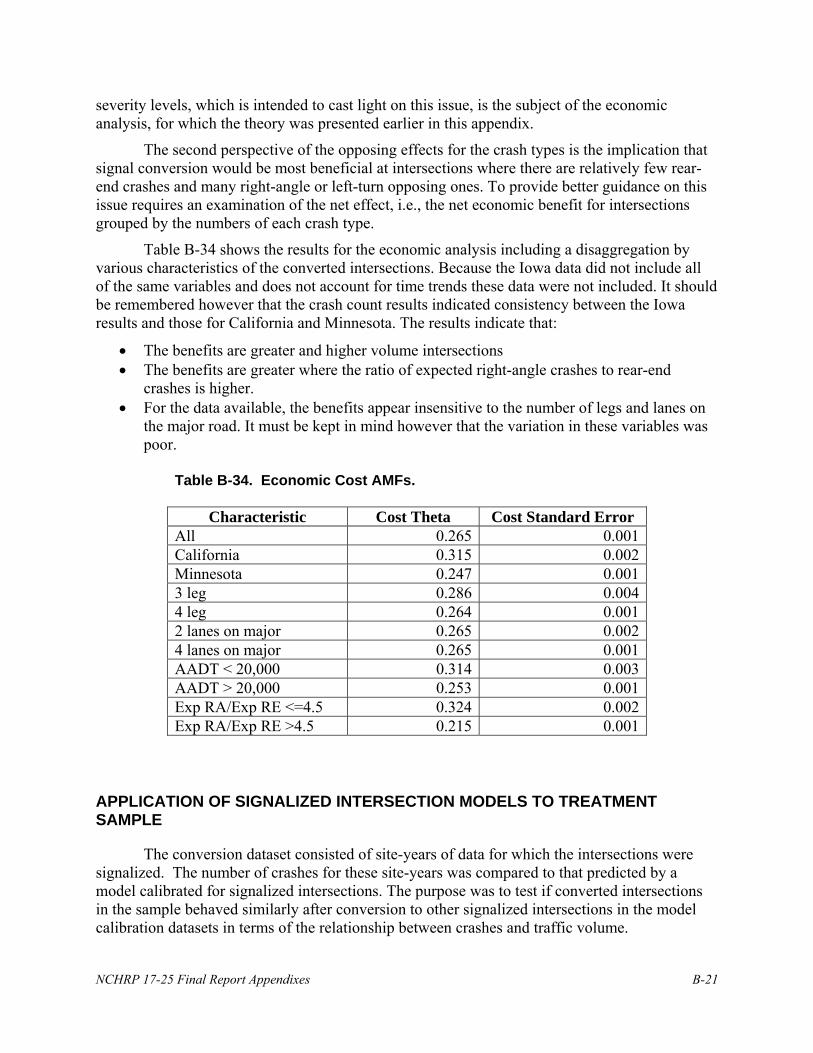
Table B-34 shows the results for the economic analysis including a disaggregation by various characteristics of the converted intersections. Because the Iowa data did not include all of the same variables and does not account for time trends these data were not included. It should be remembered however that the crash count results indicated consistency between the Iowa results and those for California and Minnesota. The results indicate that:

• The benefits are greater and higher volume intersections • The benefits are greater where the ratio of expected right-angle crashes to rear-end

crashes is higher. • For the data available, the benefits appear insensitive to the number of legs and lanes on

the major road. It must be kept in mind however that the variation in these variables was poor.

Table B-34. Economic Cost AMFs.

Characteristic Cost Theta Cost Standard Error All 0.265 0.001 California 0.315 0.002 Minnesota 0.247 0.001 3 leg 0.286 0.004 4 leg 0.264 0.001 2 lanes on major 0.265 0.002 4 lanes on major 0.265 0.001 AADT < 20,000 0.314 0.003 AADT > 20,000 0.253 0.001 Exp RA/Exp RE <=4.5 0.324 0.002 Exp RA/Exp RE >4.5 0.215 0.001

APPLICATION OF SIGNALIZED INTERSECTION MODELS TO TREATMENT SAMPLE

The conversion dataset consisted of site-years of data for which the intersections were signalized. The number of crashes for these site-years was compared to that predicted by a model calibrated for signalized intersections. The purpose was to test if converted intersections in the sample behaved similarly after conversion to other signalized intersections in the model calibration datasets in terms of the relationship between crashes and traffic volume.


The results, shown in Table B-35, are promising. Results for total, right angle and rear-end crashes perform well. It could be concluded with caution that the close correspondence between the observed and predicted crashes using the signalized reference group model is ample indication that converted intersections in the sample behave similar to other signalized intersections in terms of the relationship between crashes and traffic volume.

Table B-35. Crashes at 4-Leg intersections after conversion. Crash Type Basis for after period crashes Crashes in after period

Observed 326 Right-angle

Estimated by signalized reference group model 383

Observed 695 Rear-end Estimated by signalized reference group model 679

Observed 1496 All Estimated by signalized reference group model 1592

These results provide some evidence that the models can be used as part of a procedure

for conducting an engineering study to assess whether or not a contemplated signal installation is warranted. In this, an empirical Bayes estimate of the expected number of crashes without signalization is compared to the number of accidents expected with signalization, the latter estimated from a regression model for signalized intersections. The elements of this procedure are presented next.

PROCEDURE FOR ESTIMATING THE SAFETY BENEFIT OF A CONTEMPLATED CONVERSION OF AN EXISTING RURAL STOP-CONTROLLED INTERSECTION TO SIGNALIZED CONTROL

The objective is to provide designers and planners with a tool to estimate the change in accident frequency expected with the conversion of a rural stop-controlled intersection to signalized control.

For this approach, which is similar to one developed for urban signalized intersections1, a Safety Performance Function (SPF) representative of the existing stop-controlled intersection is required. This will require that one exists for the jurisdiction or that data are available to enable a recalibration of a model calibrated for another jurisdiction. The SPF would be used, along with the intersection’s accident history, in the empirical Bayes procedure to estimate the expected accident frequency with the status quo in place, which would then be compared to the expected frequency should a conversion to signalized control take place to estimate the expected benefit. 1 McGee H, Persaud B. and S. Taori. “Crash Experience Warrant for Traffic Signals”. National Cooperative Highway Research Program (NCHRP) Report 491, Transportation Research Board, 2003.


The expected frequency should conversion to signalized control take place is estimated from an SPF representative of signal controlled intersections in the same jurisdiction. Again, this will require that one exists for the jurisdiction or that data are available to enable a recalibration of a model calibrated for another jurisdiction. The approach is convenient, in that a comprehensive set of accident modification factors, which would be required for a large number of conditions, including AADT levels, is simply not available and is difficult to obtain.

Overview of the approach

Step 1:

Assemble data and accident prediction models for rural stop-controlled and signalized intersections. For the past, say, five years,

1. Obtain the count of total, right-angle and rear-end accidents which occurred at the intersection of interest,

2. For the same time period obtain or estimate the average AADTs on the major and minor roadways,

3. Estimate the average AADTs on the major and minor roads that would prevail for the period immediately after conversion to signal control,

4. Assemble required accident prediction models for rural stop-controlled intersections and rural signal controlled intersections. If the models cannot be assumed to be representative of the jurisdiction, they must be recalibrated using data from a sample of intersections representative of that jurisdiction. At a minimum, data for at least 10 intersections with at least 60 accidents is needed. The re-calibration multiplier is simply the number of crashes recorded in the sample divided by the number of crashes predicted for the sample by the model.

Step 2:

Use the EB procedure with the data from Step 1 and the stop-controlled intersection model to estimate the expected annual number of right-angle, rear-end and “other” accidents that would occur without conversion. (The EB estimate for “other” crashes is the EB estimate for total minus the sum of the EB estimates for rear end and right angle crashes.)

Step 3:

Use the signalized intersection models and the volumes from Step 1 to estimate the expected number of rear-end, right-angle and other crashes that would occur if the intersection were converted. (The estimate for “other” is the estimate for total minus the sum of the estimates for rear-end and right-angle.)

Step 4:

Obtain for rear-end, right-angle and “other” crashes, the difference between the estimates from Steps 2 and 3 and check that any estimated reduction in right-angle crashes is statistically significant.


Step 5:

Applying suitable severity weights and dollar values for rear-end, right-angle, and other crashes, obtain a net benefit of signal installation.

Step 6:

Compare against the cost, considering other impacts if desired, and using conventional economic analysis tools. How this is done, and in fact whether it is done, is very jurisdiction-specific and conventional methods of economic analysis can be applied after obtaining estimates of the economic values of changes in delay, fuel consumption and other impacts.

Example

A rural four-leg stop-controlled intersection with data from January 2001 to December

2005, is being considered for signal installation. Data and results of the analysis are displayed in Tables 1-3.

Example Step 1:

Assemble data and crash prediction models

a) Crash data – The counts of total, right angle and rear-end crashes in each year of the analysis period are shown in the second row of Tables B-36 through B-38.

b) AADT data – Entering AADTs for the major and minor roads for each year are estimated for each year using suitable methods applied locally and are entered in the 3rd and 4th rows of Tables B-36 through B-38. It is recognized that actual counts are typically not available for each year; however, in most jurisdictions trend factors are available that could be applied to estimate AADTs for each year. A separate process can be used to provide the best estimate of the AADT after signalization, considering traffic that might be generated to the intersection in the future. In the absence of such an estimate, the AADT expected after signalization can be assumed to be same as that in the last year.

c) Crash prediction models – For this example, these are required for rural 4-leg stop controlled intersections for each of the years 2001 to 2005 and for rural signalized 4-leg intersections for the last full year. Ideally each jurisdiction would have its own set of applicable models. The models adopted for this example are shown below in Tables B-39 and B-40.


Table B-36. Summary of results for total crashes. 1) Year (y) 2001 2002 2003 2004 2005 2) Crashes in year (X) 4 9 8 14 7 Sum = Xb = 42 3) MAJAADT 24000 25500 26000 28000 300004) MINAADT 2500 2550 2650 2800 30005) Recalibrated α × 10-4 1.03 1.05 1.07 1.09 1.116) Parameter K 0.483 0.483 0.483 0.483 0.4837) Model Prediction E{κy} 6.3 6.8 7.1 7.9 8.78) Ci,y = E{κy}/ E{κ2001} 0.72 0.78 0.82 0.90 1.009) Comp. Ratio for period ∑Ci,y = 4.22 10) Expected annual crashes without signalization (and variance) in 2005

κ(2005) = Ci,2005(1/K+ Xb)/((1/K)/E{κ2005}+∑Ci,y) = 1.00(1/0.483+42)/((1/0.483)/8.7+4.22) = 9.9 Var[κ(2005)] = (Ci,2005)/(1/K+ Xb)/(1/K/ E{κ2005}+∑Ci,y)2 = (1.00)(1/0.483+42)/(1/0.483/8.7+4.22)2 = 2.2

11) Expected annual crashes after signalization (and variance) in 2005

E{κ2005}=0.010245(300000.443)(30000.2237) = 5.9 Var[E{κ2005}]= 0.373(5.9)2 = 13.0


Table B-37. Summary of results for right-angle crashes. 1) Year (y) 2001 2002 2003 2004 2005 2) Crashes in year (X) 2 4 5 7 4 Sum = Xb = 22 3) MAJAADT 24000 25500 26000 28000 30000 4) MINAADT 2500 2550 2650 2800 3000 5) Recalibrated α × 10-4 0.330 0.337 0.343 0.350 0.357 6) Parameter K 1.128 1.128 1.128 1.128 1.128 7) Model Prediction E{κy} 2.5 2.6 2.8 3.1 3.4 8) Ci,y = E{κy}/ E{κ2001} 0.72 0.77 0.81 0.90 1.00 9) Comp. Ratio for period ∑Ci,y = 4.19 10) Expected annual crashes without signalization (and variance) in 2005



E{κ2005}=0.018369(30000*3000)0.1976 = 0.7 Var[E{κ2005}]= 0.511(0.7)2 = 0.25


Table B-38. Summary of results for rear-end crashes. 1) Year (y) 2001 2002 2003 2004 2005 2) Crashes in year (X) 1 2 3 4 0 Sum = Xb = 10 3) MAJAADT 24000 25500 26000 28000 30000 4) MINAADT 2500 2550 2650 2800 3000 5) Recalibrated α × 10-4 0.01 0.01 0.01 0.01 0.01 6) Parameter K 0.726 0.726 0.726 0.726 0.726 7) Model Prediction E{κy} 1.2 1.4 1.4 1.6 1.8 8) Ci,y = E{κy}/ E{κ2001} 0.68 0.75 0.79 0.89 1.00 9) Comp. Ratio for period ∑Ci,y = 4.11 10) Expected annual crashes without signalization (and variance) in 2005



E{κ2005}=0.000812(300000.5791)(30000.2718) = 2.8 Var[E{κ2005}]= 0.505(2.8)2 = 3.96

Table B-39. SPFs for California stop-controlled intersections (4-leg with 2 lanes on major approach). Total Right-Angle Rear-End Model 1 1 2 LN(α) (standard error)

-9.1488 (0.554)

-10.2351 (0.9337

-13.6527 (0.7938)


0.7191 (0.060)

0.5707 (0.099

1.4201 (0.088)


0.4813 (0.028)

0.6978 (0.047

0.1857 (0.041)

Dispersion, K 0.483 1.128 0.726



ββκ α

⎛ ⎞= + ⎜ ⎟

+⎝ ⎠


Table B-40. SPFs for California signalized intersections (4-leg). Total Right-Angle Rear-End Model 1 2 1 LN(α) (standard error)

-4.0402 (0.1267)

-2.6105 (1.1337)

-6.7249 (1.4141.)


0.4430 (0.1297)

0.1976 (0.0655)

0.5791 (0.1425)


0.2237 (0.0520)

0.2718 (0.0572)

State (standard error)

CA = -0.5407 (0.1402) Minnesota = 0

CA = -1.3866 (0.1725) Minnesota = 0

CA = -0.3903 (0.1687) Minnesota = 0

Dispersion, K 0.3733 (0.561)

0.5110 (0.0931)

0.5051 (0.0793)

Model 1. 1 2/ ( ) ( ) stateAcc yr Major AADT Minor AADT eβ βα=

Model 2. / ( x ) stateAcc yr Major AADT Minor AADT eβα=

It is recommended that these models be recalibrated for each jurisdiction and for each year of the analysis period. To do so requires yearly crash counts and AADTs for a sample of intersections in the jurisdiction that are typical of those that tend to be considered for signal installation. The default base model is used to estimate crashes each year for each intersection in the sample. For each year, the sum of the observed counts divided by the sum of the model estimates gives a calibration factor that is applied to the model to obtain a recalibrated value of α. These recalibrated values of α for the current illustration are shown in row 5 of Tables B-7 through B-9. A similar recalibration process can be done to adjust the α parameter for the signalized intersection model for the year 2005. In this example, it is assumed that this adjustment was not necessary.

Example Step 2:

a) Estimate the expected number of crashes per year using the recalibrated SPFs. For example, for 2001,

E{κ2001}total = (0.000103)(41302)0.7191(3596)0.4813 = 6.3

E{κ2001}right angle = (0.000033)(41302)0.5707(3596)0.6978 = 2.5

E{κ2001}rear end = (0.000001)(41302+3596)1.4201(3596/(41302+3596))0.1857 = 1.2

These estimates are shown in row 7 of Tables B-36 through B-38.


b) Calculate the comparison ratio (Ci,y) of the model estimate for a given year divided by the model estimate for 2005. These ratios are shown in row 8 of Tables B-36 through B-38 and summed in row 9.

c) Using the values in the previous rows and the formula show in the tables estimate the expected annual number of crashes without signalization (and variance) for the last year (2005). These values are shown in row 10 of Tables B-36 through B-38.

Example Step 3:

Use the signalized intersection SPFs (reproduced in Table B-41) to estimate the number of crashes per year if the intersection were signalized using the expected annual AADTs after signalization. For this example, the year 2005 is used to correspond with the estimates from Step 2 and it was assumed that a recalibration of the default base models were not required.

Also estimate the variance of the estimate as:

Var[E{κ2005}]= K(E{κ2005}2)

Table B-41. SPFs for Signalized Intersections (4-leg).

All Right-Angle Rear-End Model 1 2 1 LN(α) (standard error)

-3.4995 (0.1267)

-3.9971 (1.1337)

-7.1152 (1.4141)


0.4430 (0.1297)

0.1976 (0.0655)

0.5791 (0.1425)


0.2237 (0.0520)

0.2718 (0.0572)

Dispersion, K 0.3733 (0.561)

0.5110 (0.0931)

0.5051 (0.0793)

Model 1. Acc/yr = α(Major AADT)β1(Minor AADT)β2

Model 2. Acc/yr = α(Major AADT*Minor AADT)β1 The results are in the row 11 of Tables B-36 through B-38. Example Step 4.

Step 4a – Estimate the change in crashes per year if the intersection was converted to a signalized intersection as follows:

Total = 9.9 – 5.9 = 4.0 (decrease)

Right-angle = 5.1 – 0.7 = 4.4 (decrease)

Rear-end = 2.3 – 2.8 = -0.5 (increase)

Other = (9.9-5.1-2.3) – (5.9-0.7-2.8) = 0.1 (decrease)


Step 4b – Test for significance of the changes in major crash types. If there is a net decrease in total crashes, check that there is an expected decrease in right angle crashes and that this change is statistically significant. If there is a net increase in total accidents, check that there is an expected increase in rear-end accidents and that this change is statistically significant. If the expected changes do not materialize or are not statistically significant at the 10% level, then safety should not be used in evaluating the impacts of signalization.

In this case there is net decrease in total accidents and an expected decrease of 4.4 right-angle accidents/year. The variance of this change in right-angle accidents is equal to the sum of the variances of the two numbers that yielded this value.

Var{κ(2005)right angle} + Var{κ(2005)signal/right angle} = 1.20+0.25 = 1.45

The standard deviation is 1.2, which means that the decrease of 4.4 is statistically significant since a value of zero lies outside of 1.64 standard deviations (for a 10% significance level).

Example Step 5

Consider the relative costs of right-angle, rear-end and other crashes.

Crash cost data is available from FHWA report number FHWA-HRT-05-051 “Crash Cost Estimates by Maximum Police-Reported Injury Severity Within Selected Crash Geometrics”. The report provides the mean and standard error of the comprehensive cost per crash for various crash types disaggregated by various combinations of maximum severity level on the KABCO scale and also disaggregated by speed limit (>=50, <=45). The disaggregation by speed limit was an attempt to control for urban versus rural environment, a variable not available in the data used to derive the cost estimates. The analysis used estimates for the >=50 mph speed category to reflect the rural conditions of the treatment sites.

The unit crash costs used for this example are reproduced in Table B-42.

Table B-42. Unit crash costs for all severities (standard errors in parentheses).

Control Type Right Angle Cost Rear End Cost Other Cost

$75,197 $32,544 $75,197 Signal ($7,747) ($6,219) ($7,747) $96,942 $10.008 $96,942 Stop

Sign ($25,619) ($4,027) ($25,619)

Using these costs and the expected crash frequencies in 2005 from Tables B1 through B-3, the estimated net annual benefit of signal installation at this intersection is estimated.


Annual Cost Without Signalization

= 5.1($96,942)+2.3($10,008)+(9.9-5.1-2.3)( $96,942)

= $759,778

Annual Cost With Signalization

= (0.7)( $75,197) + (2.8)( $32,544)+( 5.9-0.7-2.8)( $75,197)

= $324,234

Annual Economic Benefit From Signalization

= $759,778 - $324,234

= $435,544

Example Step 6

Compare cost of signal installation against the benefits, considering operational benefits as well. How this is done is very jurisdiction specific and conventional methods of economic analysis can be applied after obtaining estimates of the economic values of changes in delay, fuel consumption and other impacts. Traffic engineering studies can be conducted and tools such as simulation can be used to estimate the changes in operational parameters, such as delay times, stops, fuel consumption, emissions, etc.

DISCUSSION AND CONCLUSIONS

The data collected and analyzed for this study clearly show that the safety benefit of signalizing an un-signalized intersection is a function of the crash history by crash type, the traffic entering the intersection on the major and minor approaches, and whether the intersection is a 3-legged T-intersection or a conventional 4-legged intersection. The available data indicated that total crashes can be reduced by signalizing an intersection with certain levels of crash frequency and traffic volumes, although individual intersections may yield contrary results.

An economic analysis reaffirms the benefits of signalization, where warranted. In particular, benefits of signalization are to be expected where the ratio of right-angle to rear-end crashes is high.

A procedure for estimating the safety benefits of a contemplated signal installation has been developed and presented and should be consider for application to supplement procedures used to decide if a signal installation meets MUTCD or other warrants.

REFERENCES

1. Hauer, E. (1997). Observational Before-After Studies in Road Safety: Estimating the Effect of Highway and Traffic Engineering Measures on Road Safety. Pergamon Press, Elseviser Science Ltd., Oxford, U.K.


2. Council, F.M., B. Persaud, C. Lyon, K. Eccles, M. Griffith, E. Zaloshnja, and T. Miller. Economic Analysis of the Safety Effects of Red Light Camera Programs and the Identification of Factors Associated with the Greatest Benefits. In Transportation Research Record: Journal of the Transportation Research Board, in publication, TRB, National Research Council, Washington, D.C., 2005.

3. Council, F., E. Zaloshnja, T. Miller, and B. Persaud, Crash Cost Estimates by Maximum

Police-Reported Injury Severity Within Selected Crash Geometries, FHWA-HRT-05-051, Federal Highway Administration, October 2005.

effects of converting rural intersections from stop...

Documents