PHYSICAL REVIEW A 95, 032705 (2017)

Effective radius of ground- and excited-state positronium in collisions with hard walls

R. Brown,* Q. Prigent, A. R. Swann,† and G. F. Gribakin‡

School of Mathematics and Physics, Queen’s University Belfast, Belfast BT7 1NN, United Kingdom(Received 3 February 2017; published 22 March 2017)

We determine effective collisional radii of positronium (Ps) by considering Ps states in hard-wall sphericalcavities. B-spline basis sets of electron and positron states inside the cavity are used to construct the statesof Ps. Accurate Ps energy eigenvalues are obtained by extrapolation with respect to the numbers of partialwaves and radial states included in the bases. Comparison of the extrapolated energies with those of a point-likeparticle provides values of the effective radius ρnl of Ps(nl) in collisions with a hard wall. We show that, for1s, 2s, and 2p states of Ps, the effective radius decreases with the increasing Ps center-of-mass momentum andfind ρ1s = 1.65 a.u., ρ2s = 7.00 a.u., and ρ2p = 5.35 a.u. in the zero-momentum limit.

DOI: 10.1103/PhysRevA.95.032705

I. INTRODUCTION

Positronium (Ps) is a light atom that consists of an electronand its antiparticle, the positron. Positron- and positronium-annihilation-lifetime spectroscopy is a widely used tool forstudying materials, e.g., for determining pore sizes andfree volume. For smaller pores the radius of the Ps atomitself cannot be neglected. This quantity was probed in arecent experiment which measured the cavity shift of thePs 1s-2p line [1], and the data calls for proper theoreticalunderstanding [2]. In this paper we calculate the eigenstates ofPs in a hard-wall spherical cavity and determine the effectivecollisional radius of Ps in 1s, 2s, and 2p states as a functionof its center-of-mass momentum.

The most common model for pore-size estimation is theTao–Eldrup model [3,4]. It considers an orthopositroniumatom (o-Ps), i.e., a Ps atom in the triplet state, confined inthe pore which is assumed to be spherical, with radius Rc. ThePs is modeled as a point particle with mass 2me in a sphericalpotential well, where me is the mass of an electron or positron.Collisions of o-Ps with the cavity walls allow for positrontwo-gamma (2γ ) annihilation with the electrons in the wall,which reduces the o-Ps lifetime with respect to the vacuum3γ -annihilation value of 142 ns. To simplify the descriptionof the penetration of the Ps wave function into the cavity wall,the radius of the potential well is taken to be Rc + �Rc, wherethe best value of �Rc has been empirically determined to be0.165 nm [5]. The model and its extensions are still widelyused for pore sizes in 1–100 nm range [6–8].

Porous materials and Ps confinement in cavities also en-abled a number of fundamental studies, such as measurementof Ps-Ps interactions [9], detection of the Ps2 molecule [10] andits optical spectroscopy [11], and measurements of the cavity-induced shift of the Ps Lyman-α (1s-2p) transition [1]. Cavitiesalso hold prospects of creating a Bose–Einstein condensate ofPs atoms and an annihilation-gamma-ray laser [12].

Seen in a wider context, the old subject of confinedatoms [13,14] has seen renewed interest in recent years

*Present address: School of Physics and Astronomy, The Universityof Manchester, Manchester M13 9PL, United Kingdom.†aswann02@qub.ac.uk‡g.gribakin@qub.ac.uk

[15–20]. Studies in this area not only serve as interestingthought experiments but also apply to real physical situations,e.g., atoms under high pressure [21,22] or atoms trapped infullerenes [23–25]. For o-Ps there is a specific question aboutthe extent to which confinement in a cavity affects its intrinsic3γ annihilation rate (see Ref. [26] and references therein).

For smaller cavities the effect of a finite radius of thetrapped particle on its center-of-mass motion cannot beignored. In fact, the radius of a composite quantum particledepends on the way this quantity is defined and probed.For example, the proton is usually characterized by itsroot-mean-squared charge radius. It is measured in elasticelectron-proton scattering [27] or using spectroscopy ofexotic atoms, such as muonic hydrogen [28] (with as yetunexplained discrepancies between these experiments). Fora particle trapped in a cavity, any practically defined radiusmay depend on the nature of its interaction with the walls.

In the present work we consider the simple problem of aPs atom confined in a hard-wall spherical cavity. The finitesize of Ps gives rise to energy shifts with respect to the energylevels of a point-like particle in the cavity. This allows us tocalculate the effective collisional radius of Ps that describesits interaction with the impenetrable cavity wall.

Ps is a hydrogen-like atom with a total mass of 2 and reducedmass of 1

2 (in atomic units). The most probable distancebetween the electron and positron in a free ground-state Psatom is 2a0, where a0 is the Bohr radius, while the meanelectron-positron separation is 3a0 [29]. For excited statesPs(nl) these quantities increase as n2. The Ps center of mass ishalfway between the two particles, so the most probable radiusof Ps(1s) is 1a0, its mean radius being 1.5a0. One can expectthat the distance of closest approach between the Ps center ofmass and the wall with which it collides will be similar to thesevalues. One can also expect that this distance will depend onthe center-of-mass momentum of the Ps atom, as it will be“squashed” when colliding with the wall at higher velocities.

A proper quantum-mechanical treatment of this problemis the subject of this work. A configuration-interaction (CI)approach with a B-spline basis is used to construct the states ofPs inside the cavity. Using these we determine the dependenceof the effective Ps radius on the center-of-mass momentum forthe 1s, 2s, and 2p states.

Of course, the interaction between Ps and cavity wallsin real materials is different from the idealized situation

2469-9926/2017/95(3)/032705(12) 032705-1 ©2017 American Physical Society

R. BROWN, Q. PRIGENT, A. R. SWANN, AND G. F. GRIBAKIN PHYSICAL REVIEW A 95, 032705 (2017)

considered here. It can be modeled by changing the electron-wall and positron-wall potentials. On the other hand, thehard-wall cavity can be used as a theoretical tool for studyingPs interactions with atoms [30]. An atom placed at the centerof the cavity will cause a shift of the Ps energy levels, whosepositions can be related to the Ps-atom scattering phase shiftsδL(K) for the Lth partial wave [31],

tan δL(K) = JL+1/2(K[Rc − ρ(K)])

YL+1/2(K[Rc − ρ(K)]), (1)

where K is the Ps center-of-mass momentum, Jν is the Besselfunction, Yν is the Neumann function, Rc is the cavity radius,and ρ(K) is the effective collisional radius of the Ps atom.

The paper is organized as follows: Section II describes thetheory and numerical implementation of the CI calculations ofthe energy levels and effective radii of Ps in a spherical cavity.In Sec. III these energies and radii are presented for a number ofcavity sizes and the dependence of the radii of Ps(1s), Ps(2s),and Ps(2p) on the Ps center-of-mass momentum is analyzed.We conclude in Sec. IV with a summary.

Unless otherwise stated, atomic units are used throughout.

II. THEORY AND NUMERICAL IMPLEMENTATION

A. Ps states in the cavity

The radial parts of the electron and positron states in anempty spherical cavity with impenetrable walls are solutionsof the Schrodinger equation

−1

2

d2Pεl

dr2+ l(l + 1)

2r2Pεl(r) = εPεl(r), (2)

where l is the orbital angular momentum, that satisfy theboundary conditions Pεl(0) = Pεl(Rc) = 0. Although Eq. (2)has analytical solutions, we obtain the solutions numericallyby expanding them in a B-spline basis,

Pεl(r) =∑

i

CiBi(r), (3)

where Bi(r) are the B splines, defined on an equispaced knotsequence [32]. A set of 40 splines of order 6 has been usedthroughout. Using B splines has the advantange that a centralatomic potential can be added in Eq. (2) to investigate Ps-atominteractions [30].

We denote the electron states by φμ(re) =r−1e Pεl(re)Ylm(e), where Ylm() is the spherical harmonic

that depends on the spherical angles , and the positron statesby φν(rp), where re (rp) is the position vector of the electron(positron) relative to the center of the cavity. For Ps in anempty cavity the two sets of states are identical. The indicesμ and ν stand for the possible orbital angular momentum andradial quantum numbers of each state.

The nonrelativistic Hamiltonian for Ps inside the cavity is

H = − 12∇2

e − 12∇2

p + V (re,rp), (4)

where V (re,rp) = −|re − rp|−1 is the Coulomb interactionbetween the electron and positron. The infinite potential of thewall is taken into account through the boundary conditions atre = rp = Rc. The Ps wave functions with a given total angular

momentum J and parity � are constructed as

�J�(re,rp) =∑μ,ν

Cμνφμ(re)φν(rp), (5)

where the Cμν are coefficients. The sum in Eq. (5) is over allallowed values of the orbital and radial quantum numbers upto infinity. Numerical calculations employ finite values of lmax

and nmax, respectively, and we use extrapolation to achievecompleteness (see below).

Substitution of Eq. (5) into the Schrodinger equation

H�J� = E�J�, (6)

leads to a matrix-eigenvalue problem

HC = EC, (7)

where the Hamiltonian matrix H has elements

〈ν ′μ′|H |μν〉 = (εμ + εν)δμμ′δνν ′ + 〈ν ′μ′|V |μν〉, (8)

εμ (εν) is the energy of the single-particle state μ (ν),and 〈ν ′μ′|V |μν〉 is the electron-positron Coulomb matrixelement. The vector C contains the expansion coefficientsCμν . Diagonalization of the Hamiltonian matrix yields theenergy eigenvalues E and the expansion coefficients. Workingexpressions for the wave function and matrix elements, inwhich the radial and angular variables are separated, are shownin Appendix A.

B. Definition of Ps effective radius

The effective Ps radius is determined from the energy shiftswith respect to the states of a point particle with the same massas Ps. We employ the notation nl[N,L] to label the states ofPs in the cavity. Here nl refers to its internal state, and [N,L]describes the state of the Ps center-of-mass motion. The meansof determining the four quantum numbers n, l, N , and L for Psstates is described in Sec. II C. Also, to obtain accurate valuesof the effective Ps radius, the energy eigenvalues E and otherexpectation values are extrapolated to the limits lmax → ∞ andnmax → ∞; this is discussed in detail in Sec. II D.

We consider each energy eigenvalue Enl[N,L] as the sum

Enl[N,L] = Eintnl + ECOM

nl[N,L], (9)

where Eintnl = −1/4n2 is the internal Ps bound-state

energy, and ECOMnl[N,L] is the energy of the center-of-mass motion.

The latter is related to the center-of-mass momentum Knl[N,L]

by

ECOMnl[N,L] = K2

nl[N,L]

2m, (10)

where m = 2 is the mass of Ps.Away from the wall the Ps wave function decouples into

separate internal and center-of-mass wave functions, viz.,

�J�(r,R) �∑m,ML

CJMlmLML

ψ intnlm(r)�COM

nl[N,L](R), (11)

where r = re − rp, R = (re + rp)/2 is the position vector ofthe Ps center of mass, and CJM

lmLMLis the Clebsch–Gordan

coefficient that couples the rotational state lm of the Ps internalmotion with that of its center-of-mass motion (LML). Since

032705-2

EFFECTIVE RADIUS OF GROUND- AND EXCITED-STATE . . . PHYSICAL REVIEW A 95, 032705 (2017)

the center of mass is in free motion, its wave function is givenby

�COMnl[N,L](R) ∝ 1√

RJL+1/2(Knl[N,L]R)YLML

(R). (12)

For a point-like particle, the quantization of the radial motion inthe hard-wall cavity of radius Rc gives Knl[N,L]Rc = zL+1/2,N ,where zL+1/2,N is the N th positive root of the Bessel functionJL+1/2(z). (For S-wave Ps, L = 0, z1/2,N = πN .) When thefinite effective radius ρnl[N,L] of the Ps atom is taken intoaccount, one has

Knl[N,L](Rc − ρnl[N,L]) = zL+1/2,N , (13)

which gives the energy (9) as

Enl[N,L] = − 1

4n2+ z2

L+1/2,N

4(Rc − ρnl[N,L])2 . (14)

This relation defines the effective collisional radius of Ps,

ρnl[N,L] = Rc − zL+1/2,N

(4Enl[N,L] + 1

n2

)−1/2

. (15)

The Ps radius thus defined may depend on the Ps center-of-mass state [N,L], as well as the cavity radius. As we show inSec. III, the radius is in fact determined only by the internalPs state nl and its center-of-mass momentum K , i.e., it can bewritten as ρnl(K).

In the present work, most of the calculations were per-formed for J� = 0+ and 1−, and cavity radii Rc = 10 a.u. and12 a.u. The value of Rc was kept small to assist convergenceof the CI expansion (5).

C. Identification of Ps states

After diagonalizing the Hamiltonian matrix and finding theenergy eigenvalues, one must determine the quantum numbersfor each state before the corresponding Ps radius ρnl[N,L]

can be calculated from Eq. (15). To facilitate this, the meanelectron-positron separation 〈r〉 and contact density 〈δ(r)〉were calculated for each state (see Appendix A for details).

The value of 〈r〉 for free Ps is twice the hydrogenic electronradius [29],

〈r〉 = 3n2 − l(l + 1). (16)

Thus, the expected mean separations for the 1s, 2s, and 2p

states are 3, 12, and 10 a.u., respectively. In practice, thecalculated separations for the 2s and 2p states are noticeablylower (see Sec. II D 2), since the free-Ps values of 〈r〉 arecomparable to the size of the cavity. Nevertheless, they areuseful for identifying the individual Ps states.

The contact density 〈δ(r)〉 is useful for distinguishingbetween s and p states, and between the s states with differentprincipal quantum number n. For s states of free Ps, the contactdensity is given by the hydrogenic electron density at theorigin [29] scaled by the cube of the reduced-mass factor,viz.,

〈δ(r)〉 = 1

8πn3. (17)

Hence, the expected contact densities of 1s and 2s states are1/8π ≈ 0.04 and 1/64π ≈ 5 × 10−3, respectively. For p and

higher-angular-momentum states the contact density is zero.In practice, the computed contact density for a p state wasobserved to be of the order of 10−8 or smaller.

Although looking at the numerical values of 〈r〉 and 〈δ(r)〉calculated for finite lmax and nmax is often sufficient fordistinguishing between the various states, their values can alsobe extrapolated to the limits lmax → ∞ and nmax → ∞, asdemonstrated in Sec. II D.

Once the internal Ps state nl has been established usingthe mean electron-positron separation and contact density, theangular-momentum and parity selection rules,

|l − L| � J � l + L, (18)

� = (−1)l+L, (19)

allow one to determine the possible values of L.Finally, for fixed n, l, and L, with the energy eigenvalues

arranged in increasing numerical order, the correspondingvalues of N are 1, 2, 3, etc.

D. Extrapolation

1. Energy eigenvalues

To obtain the most precise values possible, the calculatedenergy eigenvalues are extrapolated to the limits lmax → ∞and nmax → ∞. To this end, each calculation was performedfor several consecutive values of lmax with fixed nmax, and thisprocess was repeated for several values of nmax. For J� = 0+we used values of lmax = 11–15 and nmax = 10–15. Due tocomputational restrictions,1 for J� = 1− it was necessary tolower the values of lmax to the range 10–14, while keepingnmax = 10–15 (Sec. II E). Extrapolation is first performed withrespect to lmax for each value of nmax, and afterwards withrespect to nmax.

The convergence of CI expansions of the type (5) iscontrolled by the Coulomb interaction between the particles. Inour case, for s states the contributions to the total energy fromelectron and positron states with orbital angular momentum l

behave as (l + 12 )−4, while for p states, as (l + 1

2 )−6 [33,34].Denoting by E(lmax,nmax) a generic unextrapolated energyeigenvalue computed with partial waves up to lmax with nmax

states in each, we can extrapolate in lmax by using fitting curvesof the form

E(lmax,nmax) = E(∞,nmax) + A(lmax + 1

2

)−3

+B(lmax + 1

2

)−4 + C(lmax + 1

2

)−5(20)

for s states, and

E(lmax,nmax) = E(∞,nmax) + A(lmax + 1

2

)−5

+ B(lmax + 1

2

)−6(21)

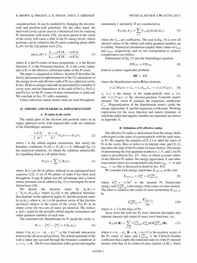
for p states, where A, B, and C are fitting parameters, andhigher-order terms are added to improve the fit. Such curveswere found to give excellent fits for our data points. Figure 1shows the extrapolation of the six lowest energy eigenvalues

1We use an x86_64 Beowulf cluster.

032705-3

R. BROWN, Q. PRIGENT, A. R. SWANN, AND G. F. GRIBAKIN PHYSICAL REVIEW A 95, 032705 (2017)

−0.25

−0.2

−0.15

−0.1

−0.05

0

0.05

0.1

0.15

0.2

0 0.0002 0.0004 0.0006

1

2

3

4

5

6

E(l

max

,nm

ax)

(a.u

.)

(lmax + 12 )−3

FIG. 1. Extrapolation in lmax for the lowest six energy eigenvaluesfor J � = 0+, Rc = 10 a.u., and nmax = 15. Solid lines connect thedata points to guide the eye, while the dashed lines show extrapolationto lmax → ∞ by using Eq. (20) or (21).

for J� = 0+, Rc = 10 a.u., and nmax = 15. The effect ofextrapolation can be seen better in Fig. 2, which shows itfor the lowest eigenvalue.

To extrapolate with respect to the maximum number ofstates in each partial wave, we assume that the incrementsin the energy with increasing nmax decrease as its negativepower. The extrapolated energy eigenvalue Enl[N,L] is thenfound from the fit

E(∞,nmax) = Enl[N,L] + αn−βmax, (22)

where α and β are fitting parameters. Again, such curvesproduced very good fits for our data points. Figure 3 showsthe extrapolation of the six lowest energy eigenvalues forJ� = 0+ and Rc = 10 a.u.

It is known that CI-type or many-body-theory calculationsfor systems containing Ps (either real or virtual) exhibit slow

−0.216

−0.215

−0.214

−0.213

−0.212

0 0.0002 0.0004 0.0006

E(l

max

,nm

ax)

(a.u

.)

(lmax + 12 )−3

FIG. 2. Extrapolation in lmax for the lowest energy eigenvalue forJ � = 0+, Rc = 10 a.u., and nmax = 15. The solid line connects thedata points to guide the eye, while the dashed line shows extrapolationto lmax → ∞ by using Eq. (20).

−0.25

−0.2

−0.15

−0.1

−0.05

0

0.05

0.1

0.15

0.2

0 0.002 0.004 0.006 0.008 0.01

1

2

3

4

5

6

E(∞

,nm

ax)

(a.u

.)

n−2max

FIG. 3. Extrapolation of the energy in nmax for the lowest sixenergy eigenvalues for J � = 0+ and Rc = 10 a.u. Solid lines connectthe data points to guide the eye, while the dashed lines showextrapolation to nmax → ∞ by using Eq. (22).

convergence with respect to the number of partial wavesincluded [35–40]. Accordingly, the extrapolation in lmax ismuch more important than the extrapolation in nmax, whichprovides only a relatively small correction. This can be seen inTable I, which shows the final extrapolated energy eigenvaluesEnl[N,L] together with E(∞,nmax) and E(lmax,nmax) obtainedfor the largest lmax and nmax values.

2. Electron-positron separation

Expectation values of the electron-positron separation 〈r〉and contact density 〈δ(r)〉 can also be extrapolated to thelimits lmax → ∞ and nmax → ∞. As with the energy, theextrapolation in nmax makes only a small correction, whichmakes it superfluous here. We only use these quantities toidentify Ps states, so precise values are not needed.

For the mean separation we used fits of the form

〈r〉[lmax] = 〈r〉 + A(lmax + 1

2

)−2 + B(lmax + 1

2

)−3(23)

for s states, and

〈r〉[lmax] = 〈r〉 + A(lmax + 1

2

)−4 + B(lmax + 1

2

)−5(24)

for p states, where 〈r〉[lmax] is the value obtained in thecalculation with a given lmax. Figure 4 shows this extrapolationfor J� = 0+, Rc = 10 a.u., and nmax = 15 for the six lowestenergy eigenvalues, along with tentative identifications of thequantum numbers n and l.

The internal Ps states were determined as follows: States1 and 2 appear to be 1s states since 〈r〉 ≈ 3 for them. State4 is also a 1s state; its 〈r〉 values for smaller lmax are closeto 3, but increasing lmax and extrapolation lead to a highervalue of 〈r〉 ≈ 4. This distortion occurs due to level mixingbetween the 1s state with L = 0 and N = 3 (state 4) and 2s

state with L = 0 and N = 1 (state 3; see below). These statesare close in energy, and the energy separation between them

032705-4

EFFECTIVE RADIUS OF GROUND- AND EXCITED-STATE . . . PHYSICAL REVIEW A 95, 032705 (2017)

TABLE I. Calculated energy eigenvalues, center-of-mass momenta, and effective radii for J� = 0+, 1− and Rc = 10 and 12 a.u.

J � Rc State no. nl[N,L] E(lmax,nmax)a E(∞,nmax)b Enl[N,L]c Knl[N,L] ρnl[N,L]

0+ 10 1 1s[1,0] −0.2144498 −0.215911 −0.216100 0.368239 1.4692 1s[2,0] −0.1174946 −0.119914 −0.120167 0.720647 1.2813 2s[1,0] 0.02472915 0.0241658 0.0239796 0.588148 4.6594 1s[3,0] 0.03396135 0.0310792 0.0309400 1.060075 1.1095 2p[1,1] 0.07686479 0.0768633 0.0768631 0.746627 3.9826 2s[2,0] 0.1511621 0.150550 0.150504 0.923047 3.193

0+ 12 1 1s[1,0] −0.2251509 −0.227540 −0.227819 0.297866 1.4532 1s[2,0] −0.1593054 −0.162912 −0.163350 0.588727 1.3283 1s[3,0] −0.05568137 −0.0601980 −0.0605930 0.870418 1.1724 2s[1,0] −0.01046464 −0.0107571 −0.0108531 0.454519 5.0885 2p[1,1] 0.02539311 0.0253906 0.0253903 0.592926 4.4226 2s[2,0] 0.07401803 0.0721989 0.0719415 0.733325 3.4327 1s[4,0] 0.08558862 0.0811920 0.0809612 1.150585 1.078

1− 10 1 1s[1,1] −0.1787461 −0.181426 −0.181500 0.523450 1.4162 1s[2,1] −0.05370988 −0.0571538 −0.0573473 0.877844 1.2003 2p[1,0] 0.004981346 0.00497852 0.00497844 0.519532 3.9534 2s[1,1] 0.08365396 0.0831681 0.0830909 0.763128 4.1125 2p[1,2] 0.1112176 0.111200 0.111199 0.833544 3.0866 1s[3,1] 0.1228439 0.118529 0.118321 1.213789 1.0167 2p[2,0] 0.1344290 0.134426 0.134425 0.887525 2.921

1− 12 1 1s[1,1] −0.2004982 −0.204725 −0.204872 0.424867 1.4242 1s[2,1] −0.1152794 −0.120225 −0.120512 0.719689 1.2663 2p[1,0] −0.02131484 −0.0213199 −0.0213201 0.405857 4.2594 1s[3,1] 0.006377168 6.09126 × 10−4 1.97942 × 10−4 1.000396 1.1005 2s[1,1] 0.02855653 0.0278117 0.0277551 0.600850 4.5226 2p[1,2] 0.05077695 0.0507504 0.0507503 0.673054 3.4377 2p[2,0] 0.06707912 0.0670723 0.0670721 0.719922 3.272

aEnergy eigenvalues obtained in the largest calculation with nmax = 15 and lmax = 15 (0+) or lmax = 14 (1−) for the positron.bEnergy eigenvalues obtained after extrapolation in lmax.cEnergy eigenvalues obtained after extrapolation in lmax and nmax.

2

3

4

5

6

7

8

0 0.002 0.004 0.006 0.008

1

2

3

4

5

6

1s

2s

2p

r(a

.u.)

(lmax + 12 )−2

FIG. 4. Extrapolation of the expected electron-positron sepa-ration in lmax for the six lowest-energy eigenstates for J � = 0+,Rc = 10 a.u., and nmax = 15. Solid lines connect the data points toguide the eye, while the dashed lines show extrapolation to lmax → ∞by using Eq. (23) or (24).

becomes smaller for lmax → ∞ (see Fig. 1). This increases theamount of level mixing and causes a noticeable decrease ofthe expectation value of 〈r〉 with lmax for state 3. This analysisis confirmed by the values of the contact density shown inSec. II D 3.

State 5 appears to be a 2p state due to the much largervalue of 〈r〉 compared with the 1s states, and also because anexcellent fit of the data points is obtained by using Eq. (24),not Eq. (23). The value of the contact density confirms this(Sec. II D 3). States 3 and 6 can be identified as 2s statesbecause their mean separations are higher than those of the1s and 2p states [cf. Eq. (16)], and the data points arefit correctly by using Eq. (23), not Eq. (24). Note that thecalculated separations for the 2s and 2p states are lower thanthe free-Ps values of 12 and 10 a.u. due to confinement by thecavity.

3. Electron-positron contact density

Expectation values of the contact density 〈δ(r)〉 provide auseful check of the identification of the Ps states. This quantityhas the slowest rate of convergence in lmax, and its extrapolation

032705-5

R. BROWN, Q. PRIGENT, A. R. SWANN, AND G. F. GRIBAKIN PHYSICAL REVIEW A 95, 032705 (2017)

0

0.005

0.01

0.015

0.02

0.025

0.03

0.035

0.04

0.045

0 0.02 0.04 0.06 0.08

1

2

3

4

5

6

1s

2s

2p

δ(r)

(a.u

.)

(lmax + 12 )−1

FIG. 5. Extrapolation of the expected contact density in lmax forthe six lowest-energy eigenstates for J � = 0+, Rc = 10 a.u., andnmax = 15. Solid lines connect the data points to guide the eye, whilethe dashed lines show extrapolation to lmax → ∞ by using Eq. (25).

uses the fit [34]

〈δ(r)〉[lmax] = 〈δ(r)〉 + A

lmax + 12

+ B(lmax + 1

2

)2 . (25)

Figure 5 shows that, for Rc = 10 a.u. and lmax = 15, extrapo-lation contributes up to 30% of the final contact-density valuesfor the six lowest-energy J� = 0+ eigenstates.

Values of the contact density confirm the state identifi-cations made in Sec. II D 2. States 1, 2, and 4 have contactdensities in the range 0.037–0.041, close to the free-Ps valueof 1/8π ≈ 0.0398 for the 1s state. State 5 has an extrapolatedcontact density of ∼10−15, confirming that it is a 2p state (forwhich the free-Ps value is zero).

States 3 and 6, which we identify as 2s sates, have contactdensities 0.018 and 0.014, respectively; the free-Ps value forthe 2s state is 1/64π ≈ 0.005, i.e., about three times smaller.The explanation for this difference is that the confining cavitycompresses the radial extent of the Ps internal wave function,thereby increasing its density at re = rp. This effect has beenobserved in calculations of radially confined Ps [41]. Theeffect of compression on the contact density of Ps in 2s statescan be estimated from the ratio of the free-Ps mean distance〈r〉 = 12 a.u. to the values obtained in our calculation (Fig. 4).The corresponding density enhancement is proportional tothe cube of this ratio, giving (12/6.9)3/64π ≈ 0.026 and(12/7.9)3/64π ≈ 0.017, for states 3 and 6, respectively, thatare close to the extrapolated densities in Fig. 5. The samecompression effect hardly affects 1s states because they aremuch more compact, and the corresponding electron-positronseparation values (for states 1 and 2) are only a little smallerthan the free-Ps value of 3 a.u. As noted earlier, the 0+ states3 (1s) and 4 (2s) exhibit some degree of level mixing, whichreduces the contact density of the former and increases that ofthe latter.

E. Eigenstates with J �= 0

Figures 1–5 show how the accurate energies, electron-positron separations, and contact densities of the six lowest-energy J� = 0+ Ps eigenstates in the cavity of radius Rc wereobtained. For this symmetry, the electron and positron orbitalangular momenta lν and lμ in the expansion (5) are equal,and the dimension of the Hamiltonian matrix in Eq. (7) is(lmax + 1)n2

max (3600 in the largest calculation). The groundstate of the system describes Ps(1s) with the orbital angularmomentum L = 0 in the lowest state of the center-of-massmotion, N = 1. Higher-lying states correspond to excitationsof the center-of-mass motion of Ps(1s) (N > 1), as well asinternal excitations of the Ps atom (2s and 2p). For 0+symmetry, the center-of-mass orbital angular momentum ofPs(2p) is L = 1, which is why this state (5 in Fig. 1) lieshigher than the lowest L = 0, N = 1 state of Ps(2s) (state 4).

We also calculated the eigenstates for a larger cavity radiusRc = 12 a.u. Increasing Rc lowers the energies of all states, andfor J� = 0+ we identify four 1s states (L = 0, N = 1–4), two2s states (L = 0, N = 1, 2), and one 2p state (L = 1, N = 1);see Table I. States that lie at higher energies, above the Psbreakup threshold [E = 0 for free Ps, or above 2π2/(2R2

c ) ∼0.1 a.u. in the cavity] do not have the form (11) but describe arelatively weakly correlated electron and positron “bouncing”inside the cavity.

To find other states of Ps(2p) we performed calculationsof J� = 1− states for both Rc = 10 and 12 a.u. For thissymmetry the electron and positron orbital angular momentaare related by lμ = lν ± 1, and the size of the Hamiltonianmatrix is 2lmaxn

2max, i.e., about a factor of two larger than

for J� = 0+. For computational reasons, it is convenient todefine lmax as the maximum angular momentum of one of theparticles, e.g., the positron. In this case the electron orbitalangular momentum can be as large as lmax + 1. Limiting itsvalue by 14, we restrict the value of lmax used for extrapolationto the range 10–13. This difference aside, extrapolation of theenergy eigenvalues and other quantities for the 1− states isperformed as described in Sec. II D. In total, we find seveneigenstates for J� = 1−: three for Ps(1s) (L = 1, N = 1–3),three for Ps(2p) (L = 1, N = 1, 2 and L = 2, N = 1), andone for Ps(2s) (L = 0, N = 1); see Table I.

III. RESULTS

Table I shows the quantum numbers and energy eigenvaluesEnl[N,L] of the J� = 0+ and 1− states we found for Rc = 10and 12 a.u. alongside the corresponding Ps center-of-massmomenta Knl[N,L] and effective Ps radii ρnl[N,L]. As expected,the values of ρnl[N,L] for the Ps(1s) states are much smallerthan those for Ps in the 2s and 2p states. The Ps radius foreach internal state also displays significant variation with thePs center-of-mass quantum numbers N and L and with thecavity radius Rc. It turns out that, to a good approximation,this variation can be analyzed in terms of a single parameter;namely, the Ps center-of-mass momentum K .

Figure 6 presents 13 values of the radius of Ps(1s) statesfrom Table I, plotted as a function of K . The figure shows that,to a very good approximation, the dependence of the Ps radius

032705-6

EFFECTIVE RADIUS OF GROUND- AND EXCITED-STATE . . . PHYSICAL REVIEW A 95, 032705 (2017)

0.8

1

1.2

1.4

1.6

1.8

0 0.2 0.4 0.6 0.8 1 1.2 1.4

Eff

ecti

vera

dius

ρ 1s(K

)(a

.u.)

Center-of-mass momentum K (a.u.)

JΠ = 0+ , Rc = 10JΠ = 0+ , Rc = 12JΠ = 1− , Rc = 10JΠ = 1− , Rc = 12

FIG. 6. Dependence of the effective Ps(1s) radius ρ1s(K) on thePs center-of-mass momentum K . The dashed line is the linear fit,Eq. (26).

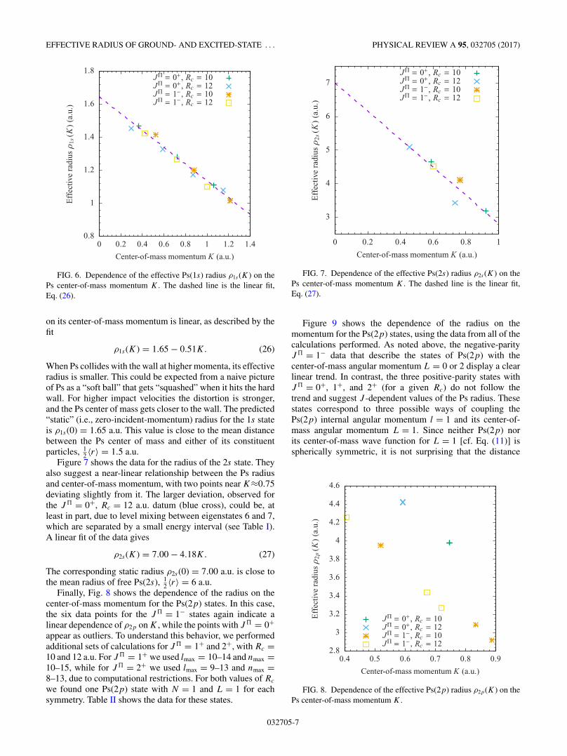
on its center-of-mass momentum is linear, as described by thefit

ρ1s(K) = 1.65 − 0.51K. (26)

When Ps collides with the wall at higher momenta, its effectiveradius is smaller. This could be expected from a naive pictureof Ps as a “soft ball” that gets “squashed” when it hits the hardwall. For higher impact velocities the distortion is stronger,and the Ps center of mass gets closer to the wall. The predicted“static” (i.e., zero-incident-momentum) radius for the 1s stateis ρ1s(0) = 1.65 a.u. This value is close to the mean distancebetween the Ps center of mass and either of its constituentparticles, 1

2 〈r〉 = 1.5 a.u.Figure 7 shows the data for the radius of the 2s state. They

also suggest a near-linear relationship between the Ps radiusand center-of-mass momentum, with two points near K≈0.75deviating slightly from it. The larger deviation, observed forthe J� = 0+, Rc = 12 a.u. datum (blue cross), could be, atleast in part, due to level mixing between eigenstates 6 and 7,which are separated by a small energy interval (see Table I).A linear fit of the data gives

ρ2s(K) = 7.00 − 4.18K. (27)

The corresponding static radius ρ2s(0) = 7.00 a.u. is close tothe mean radius of free Ps(2s), 1

2 〈r〉 = 6 a.u.Finally, Fig. 8 shows the dependence of the radius on the

center-of-mass momentum for the Ps(2p) states. In this case,the six data points for the J� = 1− states again indicate alinear dependence of ρ2p on K , while the points with J� = 0+appear as outliers. To understand this behavior, we performedadditional sets of calculations for J� = 1+ and 2+, with Rc =10 and 12 a.u. For J� = 1+ we used lmax = 10–14 and nmax =10–15, while for J� = 2+ we used lmax = 9–13 and nmax =8–13, due to computational restrictions. For both values of Rc

we found one Ps(2p) state with N = 1 and L = 1 for eachsymmetry. Table II shows the data for these states.

3

4

5

6

7

0 0.2 0.4 0.6 0.8 1

Eff

ecti

vera

dius

ρ 2s(K

)(a

.u.)

Center-of-mass momentum K (a.u.)

JΠ = 0+ , Rc = 10JΠ = 0+ , Rc = 12JΠ = 1− , Rc = 10JΠ = 1− , Rc = 12

FIG. 7. Dependence of the effective Ps(2s) radius ρ2s(K) on thePs center-of-mass momentum K . The dashed line is the linear fit,Eq. (27).

Figure 9 shows the dependence of the radius on themomentum for the Ps(2p) states, using the data from all of thecalculations performed. As noted above, the negative-parityJ� = 1− data that describe the states of Ps(2p) with thecenter-of-mass angular momentum L = 0 or 2 display a clearlinear trend. In contrast, the three positive-parity states withJ� = 0+, 1+, and 2+ (for a given Rc) do not follow thetrend and suggest J -dependent values of the Ps radius. Thesestates correspond to three possible ways of coupling thePs(2p) internal angular momentum l = 1 and its center-of-mass angular momentum L = 1. Since neither Ps(2p) norits center-of-mass wave function for L = 1 [cf. Eq. (11)] isspherically symmetric, it is not surprising that the distance

2.8

3

3.2

3.4

3.6

3.8

4

4.2

4.4

4.6

0.4 0.5 0.6 0.7 0.8 0.9

Eff

ecti

vera

dius

ρ 2p

(K)

(a.u

.)

Center-of-mass momentum K (a.u.)

JΠ = 0+ , Rc = 10JΠ = 0+ , Rc = 12JΠ = 1− , Rc = 10JΠ = 1− , Rc = 12

FIG. 8. Dependence of the effective Ps(2p) radius ρ2p(K) on thePs center-of-mass momentum K .

032705-7

R. BROWN, Q. PRIGENT, A. R. SWANN, AND G. F. GRIBAKIN PHYSICAL REVIEW A 95, 032705 (2017)

TABLE II. Calculated energy eigenvalues, center-of-mass mo-menta, and effective radii for J � = 1+, 2+ and Rc = 10 and 12 a.u.Only the Ps(2p) states are shown.

J � Rc State no. [N,L] E2p[N,L] K2p[N,L] ρ2p[N,L]

1+ 10 1 [1,1] 0.0477391 0.664045 3.2331+ 12 1 [1,1] 0.00718021 0.527940 3.4892+ 10 3 [1,1] 0.0576334 0.693205 3.5182+ 12 3 [1,1] 0.0134862 0.551312 3.850

of closest approach to the wall (i.e., the Ps radius) dependson the asymmetry of the center-of-mass motion through J . Asimple perturbative estimate of the J splitting of these statesis provided in Appendix B.

To define a spherically averaged collisional radius of Ps(2p)we take a weighted average of these data (KJ ,ρ2p[1,1]J ) withweights 2J + 1 for each Rc. The corresponding values areshown by diamonds in Fig. 9. They lie close to the J� = 2+data points (see Appendix B for an analytical explanation), andagree very well with the momentum dependence predicted bythe J� = 1− data. Using these together gives the linear fit

ρ2p(K) = 5.35 − 2.77K. (28)

The static radius for the 2p state ρ2p(0) = 5.35 a.u. is againclose to the mean radius of free Ps(2p), i.e., 1

2 〈r〉 = 5 a.u.Regarding J� = 1− data, the Ps(2p) radii in the states with

L = 0 (two for each of Rc) are naturally spherically averaged.The J� = 1− states with L = 2 are parts of the J -dependentmanifold (J = 1, 2, and 3). Here it appears that the J = 1state here is close to the J -averaged value (see Appendix B),so that all J� = 1− data follow the same linear momentumdependence.

2.5

3

3.5

4

4.5

5

5.5

0 0.2 0.4 0.6 0.8

Eff

ecti

vera

dius

ρ 2p

(K)

(a.u

.)

Center-of-mass momentum K (a.u.)

J Π = 0+ , R c = 10J Π = 0+ , R c = 12J Π = 1− , R c = 10J Π = 1− , R c = 12J Π = 1+ , R c = 10J Π = 1+ , R c = 12J Π = 2+ , R c = 10J Π = 2+ , R c = 12weighted average for Π = 1, R c = 10weighted average for Π = 1, R c = 12

FIG. 9. Dependence of the effective Ps(2p) radius ρ2p(K) on thePs center-of-mass momentum K , including data for J� = 1+ and 2+

states. The dashed line is the linear fit, Eq. (28).

Estimate of cavity shift of Lyman-α transition

Measurements of the Ps Lyman-α transition in poroussilica revealed a blueshift of the transition energy �E =1.26 ± 0.06 meV [1]. The pore size in this material is estimatedto be a ∼ 5 nm [42]. Assuming spherical pores for simplicity,we find their radius Rc ∼ 50 a.u. The Ps center-of-massmomentum in the lowest-energy state in such pores is K �π/Rc ∼ 0.06 a.u. For such a small momentum one can usestatic values of the Ps radius in 1s and 2p states (see Figs. 6and 9). Considering S-wave Ps (L = 0), we estimate the cavityshift of the Lyman-α transition energy from Eq. (14),

�E � π2

2R3c

(ρ2p − ρ1s). (29)

For static radii ρ1s = 1.65 a.u. and ρ2p = 5.35 a.u., and Rc =50 a.u., we obtain �E = 4 meV. This value is close to thenaive estimate that uses mean Ps radii [1] and is significantlylarger than the experimental value.

It appears from the measured �E that the radius of Ps(2p)is only slightly greater than that of Ps(1s). This effect islikely due to the nature of the Ps interaction with the wall ina real material. The Ps(2p) state is degenerate with Ps(2s),and their linear combination (a hydrogenic eigenstate inparabolic coordinates [29]) can possess a permanent dipolemoment. Such a state can have a stronger, more attractiveinteraction with the cavity wall than the ground-state Ps(1s).This interaction will result in an additional phase shift of thePs center-of-mass wave function reflected by the wall. Thescattering phase shift δnl(K) is related to the Ps radius ρnl(K)by δnl(K) = −Kρnl(K) [cf. Eq. (13)], with the static radiusρnl(0) playing the role of the scattering length. It is known thatthe van der Waals interaction between the ground-state Ps andnoble-gas atoms can significantly reduce the magnitude of thescattering length [30,43–45]. It can be expected that a similardispersive interaction between excited-state Ps and the cavitywall can reduce the effective radius of Ps(2p) by more thanthat of Ps(1s), to produce the difference ρ2p − ρ1s ≈ 1 a.u.compatible with experiment.

IV. CONCLUSIONS

A B-spline basis was employed to obtain single-particleelectron and positron states within an otherwise empty spheri-cal cavity. These states were used to construct the two-particlestates of positronium, including only finitely many partialwaves and radial states in the expansion. Diagonalization ofthe Hamiltonian matrix allowed us to determine the energyand expectation values of the electron-positron separation andcontact density for each state. Extrapolation of the energywith respect to the maximum orbital angular momentum lmax

and the number of radial states nmax included for each partialwave was carried out. The electron-positron separation andcontact density values were also extrapolated with respect tothe number of partial waves included and used to determinethe nature (i.e., the quantum numbers) of each positroniumstate. From the extrapolated energies, the effective collisionalradius of the positronium atom was determined for eachstate.

032705-8

EFFECTIVE RADIUS OF GROUND- AND EXCITED-STATE . . . PHYSICAL REVIEW A 95, 032705 (2017)

We have found that the radius of the Ps atom in theground state has a linear dependence on the Ps center-of-mass momentum, Eq. (26), the radius being smaller forhigher-impact momenta. The radius of Ps(2s) also displaysa linear momentum dependence, Eq. (27). The static (i.e.,zero-momentum) collisional radii of the 1s and 2s states are1.65 and 7 a.u., respectively. Determining the effective radiusof Ps in the 2p state is more complex due to its asymmetry.Spherically averaged values of the collisional radius areobtained directly for Ps S-wave states in the cavity, withPs D-wave states giving similar radii. However, determiningthe corresponding values for the Ps P -wave states requiredaveraging over the total angular momentum of the Ps states inthe cavity. (See Appendix B for a quantitative explanation forthe J dependence of the 2p[1,1] and 2p[1,2] energy levels.)After this, all data points were found to follow the lineardependence on the Ps momentum, giving the static radius of5.35 a.u. In all three cases, the static values of the effective Psradius are close to the expectation value of the radius of freePs, i.e., a half of the mean electron-positron separation.

While the linear fits obtained here for the dependence ofthe effective Ps radius on the center-of-mass momentum areclearly very good, particularly for the 1s state, it must benoted that there is a certain amount of scatter around thelines. This phenomenon may be due to numerical errors inthe two-particle-state calculations or in the extrapolation ofthe energy eigenvalues (or both). The main issue here is theslow convergence of the single-center expansion for statesthat describe the compact Ps atom away from the origin.This issue also prevented us from performing calculations forlarger-sized cavities, which would provide effective Ps radiifor lower center-of-mass momenta. A possible means to reducethe scatter in the data and tackle large cavities could be toinclude more partial waves and radial states per partial wavein the CI expansion. However, with the Hamiltonian matrixdimensions increasing as lmaxn

2max, this quickly becomes

computationally expensive. An alternative would be to usea variational approach with explicitly correlated two-particlewave functions.

Although we have only considered the 1s, 2s, and 2p

states in the present work, it is possible to use the method toinvestigate the effective radii of higher excited states, e.g., the3s, 3p, and 3d states. However, this would require calculationswith much larger cavities that can fit the n = 3 Ps states withoutsignificantly squeezing them.

It was noted earlier that confinement can cause a Ps atom to“shrink” from its size in vacuo. This manifests in the form ofa reduced electron-positron separation and increased contactdensity; these effects were observed for the 2s and 2p states.While this is true in an idealized hard-wall cavity, in physicalcavities (e.g., in a polymer) there is a second, competingeffect. Polarization of the Ps atom by the surrounding mattermay actually lead to a swollen Ps atom, which causes thecontact density to be reduced from its value in vacuo [46,47].Experimentally, it has generally been found that the net resultof these two effects is that the contact density is reducedfrom its in vacuo value, although increased values are notnecessarily impossible [47,48]. It may be possible to determinemore physical effective Ps radii by using realistic electron- andpositron-wall potentials in place of the hard wall we have used

here. Such development of the approach adopted in the presentwork should yield much more reliable data for the distorted Psstates than crude model calculations [26].

The technique outlined in this paper is eminently suitablefor implementing a bound-state approach to low-energy Ps-atom scattering. By calculating single-particle electron andpositron states in the field of an atom at the center of the cavity(rather than the empty cavity) and constructing two-particle Pswave functions from these, a shifted set of energy levels may befound. From these, the Ps-atom scattering phase shifts can bedetermined [cf. Eq. (1)] using the now known collisional radiusof Ps. We have carried out several preliminary calculationsin this area for elastic Ps(1s)-Ar scattering at the static(Hartree–Fock) level and found a scattering length of 2.85 a.u.,in perfect agreement with an earlier fixed-core stochasticvariational method calculation in the static approximation byMitroy and Ivanov [43]. This provides evidence that the linearfits presented here account for the finite size of the Ps atom inscattering calculations very accurately. In our calculations wehave also observed fragmented Ps states at higher energies (thismanifests as a larger-than-usual electron-positron separation).These have been ignored in the present work, but it may bepossible to use them to obtain information about inelasticscattering using this method.

It is hoped that the results presented here will be of use infuture studies of both confined positronium and positronium-atom scattering.

ACKNOWLEDGMENTS

We are grateful to D. G. Green for helpful comments andsuggestions. The work of A.R.S. has been supported by theDepartment for the Economy, Northern Ireland.

APPENDIX A: WORKING EXPRESSIONS FORHAMILTONIAN MATRIX AND EXPECTATION VALUES

Written in terms of the angular and radial parts of theelectron and positron basis states, the Ps wave function is

�J�(re,rp) = 1

rerp

∑μ,ν

mμ,mν

C(J )μν Pμ(re)Pν(rp)

× CJMlμmμlνmν

Ylμmμ(e)Ylνmν

(p), (A1)

where CJMlμmμlνmν

is the Clebsch–Gordan coefficient, and theindices μ and ν enumerate the radial electron and positronbasis states with various orbital angular momenta, μ ≡ εμlμand ν ≡ ενlν . Besides the selection rules due to the Clebsch–Gordan coefficient, the summation is restricted by parity,(−1)lμ+lν = �, where � = 1 (−1) for the even (odd) states.

Integration over the angular variables in the Coulombmatrix elements is performed analytically [49], and theHamiltonian matrix elements for the Ps states with the totalangular momentum J are given by

H(J )μ′ν ′,μν = (εμ + εν)δμμ′δνν ′ + V

(J )μ′ν ′,μν, (A2)

032705-9

R. BROWN, Q. PRIGENT, A. R. SWANN, AND G. F. GRIBAKIN PHYSICAL REVIEW A 95, 032705 (2017)

where

V(J )μ′ν ′,μν =

∑l

(−1)J+l

{J lμ′ lν ′

l lν lμ

}〈ν ′μ′‖Vl‖μν〉, (A3)

and the reduced Coulomb matrix element is

〈ν ′μ′‖Vl‖μν〉 = √[lν ′][lμ′][lμ][lν]

(lμ′ l lμ0 0 0

)

×(

lν ′ l lν0 0 0

)∫ Rc

0

∫ Rc

0Pν ′(rp)Pμ′(re)

× rl<

rl+1>

Pμ(re)Pν(rp) dre drp, (A4)

with [l] ≡ 2l + 1, r< = min(re,rp), and r> = max(re,rp).The expectation value of the electron-positron separation

rep = |re − rp| for an eigenstate with eigenvector C(J )μν is found

as

〈rep〉 =∑μ′,ν ′μ,ν,l

C(J )μ′ν ′C

(J )μν (−1)J+l

{J lμ′ lν ′

l lν lμ

}〈ν ′μ′‖Sl‖μν〉,

(A5)

where

〈ν ′μ′‖Sl‖μν〉 = √[lν ′][lμ′][lμ][lν]

(lμ′ l lμ0 0 0

)

×(

lν ′ l lν0 0 0

) ∫ Rc

0

∫ Rc

0Pν ′ (rp)Pμ′(re)

× rl<

rl+1>

(r2<

2l + 3− r2

>

2l − 1

)Pμ(re)

×Pν(rp) dre drp. (A6)

Similarly, the expectation value of the electron-positroncontact density δep = δ(re − rp) is

〈δep〉 =∑μ′,ν ′μ,ν,l

C(J )μ′ν ′C

(J )μν (−1)J+l

{J lμ′ lν ′

l lν lμ

}〈ν ′μ′‖δl‖μν〉,

(A7)

where

〈ν ′μ′‖δl‖μν〉 =√

[lν ′][lμ′

][lμ][lν]

(lμ′ l lμ0 0 0

)

×(

lν ′ l lν0 0 0

)[l]

4π

∫ Rc

0Pν ′ (r)Pμ′(r)Pμ(r)

×Pν(r)dr

r2. (A8)

APPENDIX B: SPLITTING OF Ps nl[N,L] STATES DUE TOINTERACTION WITH CAVITY WALL

The angular part of the Ps wave function in the cavity,Eq. (11), is

�(J )lL (r,R) =

∑m,ML

CJMlmLML

Ylm(r)YLML(R). (B1)

The electron and positron repulsion from the wall is strongestwhen the vectors r and R are parallel or antiparallel. Inthe simplest approximation, we can take the correspondingperturbation as being proportional to cos2 θ , where θ is theangle between r and R. Shifting this by a constant to make thespherical average of the perturbation zero, we write it as

δV (r,R) = αP2(cos θ ), (B2)

where α is a constant that can depend on the quantum numbersn and N and on the cavity radius Rc, and P2 is the secondLegendre polynomial. The corresponding energy shift is

�E(pert)J = α

∫∫ ∣∣�(J )lL (r,R)

∣∣2P2(cos θ ) dr dR, (B3)

by first-order perturbation theory. Integrating over the angles,one obtains [49]

�E(pert)J = α(2l + 1)(2L + 1)

(l 2 l

0 0 0

)(L 2 L

0 0 0

)

× (−1)J{L l J

l L 2

}

= α(2l + 1)(2L + 1)

(l 2 l

0 0 0

)(L 2 L

0 0 0

)

TABLE III. Comparison of the energy shifts �EJ obtained from the numerical eigenvalues EJ with the perturbative estimates �E(pert)J ,

Eq. (B4), for Ps(2p) states with N = 1 and L = 1, 2, for cavity radii Rc = 10 and 12 a.u.

nl[N,L] Rc J � EJ 〈EJ 〉 �EJ �E(pert)J /α α �E

(pert)J

2p[1,1] 10 0+ 0.0768631 0.0203912 2/5 0.0190221+ 0.0477391 0.0564719 −0.0087328 −1/5 0.047556 −0.0095112+ 0.0576334 0.0011615 1/25 0.001902

12 0+ 0.0253903 0.0126834 2/5 0.0119151+ 0.00718021 0.0127069 −0.0055267 −1/5 0.029787 −0.0059572+ 0.0134862 0.0007793 1/25 0.001191

2p[1,2] 10 1− 0.111199 −0.000037 1/5 0.0080452− 0.103201 0.111236 −0.008035 −1/5 0.040224 −0.0080453− 0.116992 0.005756 2/35 0.002299

12 1− 0.0507503 0.0008605 1/5 0.0053572− 0.0443476 0.0498898 −0.0055422 −1/5 0.026787 −0.0053573− 0.0534797 0.0035899 2/35 0.001531

032705-10

EFFECTIVE RADIUS OF GROUND- AND EXCITED-STATE . . . PHYSICAL REVIEW A 95, 032705 (2017)

−0.01

−0.005

0

0.005

0.01

0.015

0.02

0.025

0 1 2 3

ΔE

J,Δ

E(p

ert)

J(a

.u.)

J

L = 1, numericalL = 1, perturbative

L = 2, numericalL = 2, perturbative

FIG. 10. Values of �EJ and �E(pert)J for the 2p[1,1] and 2p[1,2]

states in a cavity of radius Rc = 10 a.u.

× (−1)l+L

√(2L − 2)! (2l − 2)!

(2L + 3)! (2l + 3)!

× (6X2 + 6X − 8Y

), (B4)

where X = J (J + 1) − l(l + 1) − L(L + 1) and Y = l(l +1)L(L + 1).

It is easy to check that the average energy shift is zero, i.e.,∑J

(2J + 1)�E(pert)J = 0, (B5)

as it should be for a perturbation with a zero spherical average,〈δV 〉 = 0.

For Ps states 2p[1,1] and 2p[1,2] the possible values of J

are 0, 1, 2 and 1, 2, 3, respectively. In each case, let EJ denotethe calculated energy eigenvalues of the J manifold, with theaverage energy

〈EJ 〉 =∑

J (2J + 1)EJ∑J (2J + 1)

. (B6)

To compare the numerical energy shifts �EJ ≡ EJ − 〈EJ 〉with �E

(pert)J , we choose α to reproduce the calculated mean-

squared shift, viz.,∑J

(2J + 1)[�E

(pert)J

]2 =∑

J

(2J + 1)[�EJ ]2. (B7)

−0.01

−0.005

0

0.005

0.01

0.015

0 1 2 3

ΔE

J,Δ

E(p

ert)

J(a

.u.)

J

L = 1, numericalL = 1, perturbative

L = 2, numericalL = 2, perturbative

FIG. 11. Values of �EJ and �E(pert)J for the 2p[1,1] and 2p[1,2]

states in a cavity of radius Rc = 12 a.u.

Table III shows the energy eigenvalues, J -averaged en-ergies, numerical and perturbative energy shifts �EJ and�E

(pert)J , as well as the values of α, for Ps(2p) states with

L = 1 and L = 2, for Rc = 10 and 12 a.u.To complete the multiplet for L = 2, calculations for J� =

2− and 3− were carried out by using lmax = 9–13 and nmax =8–13. For a given Rc the values of α for L = 1 and 2 statesare similar. On the other hand, when Rc increases from 10 to12 a.u., the values of α decrease as 1/R

qc with q ∼ 2.5. This

is close to the expected 1/R3c dependence of the energy shifts

with the cavity radius [2].Figures 10 and 11 compare the values of �EJ with

their perturbative estimates �E(pert)J for Rc = 10 and 12 a.u.

respectively.For L = 1 the perturbative estimates of the energy shifts are

in excellent agreement with their numerical counterparts. Notethat the small shift of the J� = 2+ level is explained by thesmall magnitude of the corresponding 6j symbol in Eq. (B4).For L = 2 states, the perturbative estimate reproduces theoverall J dependence of the calculated energy shift, with theJ = 2 state being the lowest of the three. However, the relativepositions of the J = 1 and J = 3 states are reversed. This isprobably due to higher-order corrections or level mixing notdescribed by Eq. (B2). Note that the numerical shift is smallestfor the J = 1 state, which justifies its use in determining thefit (28).

[1] D. B. Cassidy, M. W. J. Bromley, L. C. Cota, T. H. Hisakado,H. W. K. Tom, and A. P. Mills, Jr., Phys. Rev. Lett. 106, 023401(2011).

[2] D. G. Green and G. F. Gribakin, Phys. Rev. Lett. 106, 209301(2011); in this paper the Ps radius is estimated as the meanelectron-positron separation 〈r〉, whereas it seems better touse 1

2 〈r〉.

[3] S. J. Tao, J. Chem. Phys. 56, 5499(1972).

[4] M. Eldrup, D. Lightbody, and J. N. Sherwood, Chem. Phys. 63,51 (1981).

[5] Positron and Positronium Chemistry, Vol. 57, edited byD. M. Schrader and Y. C. Jean (Elsevier, New York,1988).

032705-11

R. BROWN, Q. PRIGENT, A. R. SWANN, AND G. F. GRIBAKIN PHYSICAL REVIEW A 95, 032705 (2017)

[6] D. W. Gidley, W. E. Frieze, T. L. Dull, A. F. Yee, E. T. Ryan,and H.-M. Ho, Phys. Rev. B 60, R5157 (1999).

[7] T. Goworek, B. Jasinska, J. Wawryszczuk, R. Zaleski, and T.Suzuki, Chem. Phys. 280, 295 (2002).

[8] K. Wada and T. Hyodo, J. Phys.: Conf. Ser. 443, 012003 (2013).[9] D. B. Cassidy and A. P. Mills, Jr., Phys. Rev. Lett. 107, 213401

(2011).[10] D. B. Cassidy and A. P. Mills, Jr., Nature (London) 449, 195

(2007).[11] D. B. Cassidy, T. H. Hisakado, H. W. K. Tom, and A. P. Mills,

Jr., Phys. Rev. Lett. 108, 133402 (2012).[12] D. B. Cassidy and A. P. Mills, Jr., Phys. Status Solidi C 4, 3419

(2007).[13] A. Michels, J. de Boer, and A. Bijl, Physica 4, 981 (1937).[14] A. Sommerfeld and H. Welker, Ann. Phys. (Berlin, Ger.) 424,

56 (1938).[15] W. Jaskolski, Phys. Rep. 271, 1 (1996).[16] A. L. Buchachenko, J. Phys. Chem. B 105, 5839 (2001).[17] J.-P. Connerade and P. Kengkan, in Proc. Idea-Finding Symp.

(Frankfurt Institute for Advanced Studies, Frankfurt, 2003) pp.35–46.

[18] J.-P. Connerade and P. Kengkan, in Electron Scattering, Physicsof Atoms and Molecules, edited by C. T. Whelan and N. J.Mason (Springer, New York, 2005), pp. 1–11.

[19] Theory of Confined Quantum Systems—Part One, Vol. 57, editedby J. R. Sabin and E. J. Brandas (Academic Press, New York,2009).

[20] Theory of Confined Quantum Systems—Part Two, Vol. 58, editedby J. R. Sabin and E. J. Brandas (Academic Press, New York,2009).

[21] J. M. Lawrence, P. S. Riseborough, and R. D. Parks, Rep. Prog.Phys. 44, 1 (1981).

[22] J. P. Connerade and R. Semaoune, J. Phys. B: At., Mol. Opt.Phys. 33, 3467 (2000).

[23] D. D. Bethune, R. D. Johnson, J. R. Salem, M. S. de Vries, andC. S. Yannoni, Nature (London) 366, 123 (1993).

[24] H. Shinohara, Rep. Prog. Phys. 63, 843 (2000).[25] K. Komatsu, M. Murata, and Y. Murata, Science 307, 238 (2005).[26] G. M. Tanzi, F. Castelli, and G. Consolati, Phys. Rev. Lett. 116,

033401 (2016).[27] A1 Collaboration, J. C. Bernauer, P. Achenbach, C. A. Gayoso,

R. Bohm, D. Bosnar, L. Debenjak, M. O. Distler, L. Doria,A. Esser, H. Fonvieille, J. M. Friedrich, J. Friedrich, M. G.Rodrıguez de la Paz, M. Makek, H. Merkel, D. G. Middleton, U.Muller, L. Nungesser, J. Pochodzalla, M. Potokar, S. S. Majos,B. S. Schlimme, S. Sirca, T. Walcher, and M. Weinriefer, Phys.Rev. Lett. 105, 242001 (2010).

[28] A. Antognini, F. Nez, K. Schuhmann, F. D. Amaro, F. Biraben,J. M. R. Cardoso, D. S. Covita, A. Dax, S. Dhawan, M. Diepold,L. M. P. Fernandes, A. Giesen, A. L. Gouvea, T. Graf, T.W. Hansch, P. Indelicato, L. Julien, C.-Y. Kao, P. Knowles,F. Kottmann, E.-O. Le Bigot, Y.-W. Liu, J. A. M. Lopes,L. Ludhova, C. M. B. Monteiro, F. Mulhauser, T. Nebel, P.Rabinowitz, J. M. F. dos Santos, L. A. Schaller, C. Schwob, D.Taqqu, J. F. C. A. Veloso, J. Vogelsang, and R. Pohl, Science339, 417 (2013).

[29] L. D. Landau and E. M. Lifshitz, Quantum Mechanics: Non-Relativistic Theory, 2nd ed. (Pergamon Press, Oxford, 1965).

[30] A. R. Swann and G. F. Gribakin, Positronium scattering bynoble-gas atoms using a spherical cavity (2017) (unpublished).

[31] P. G. Burke, Potential Scattering in Atomic Physics (Springer,New York, 1977).

[32] C. de Boor, A Practical Guide to Splines, Vol. 27, revised ed.(Springer, New York, 2001).

[33] W. Kutzelnigg and J. D. Morgan, J. Chem. Phys. 96, 4484 (1992).[34] G. F. Gribakin and J. Ludlow, J. Phys. B: At., Mol. Opt. Phys.

35, 339 (2002).[35] I. Bray and A. T. Stelbovics, Phys. Rev. A 48, 4787 (1993).[36] G. F. Gribakin and J. Ludlow, Phys. Rev. A 70, 032720

(2004).[37] J. Mitroy and M. W. J. Bromley, Phys. Rev. A 73, 052712

(2006).[38] M. C. Zammit, D. V. Fursa, and I. Bray, Phys. Rev. A 87, 020701

(2013).[39] D. G. Green and G. F. Gribakin, Phys. Rev. A 88, 032708 (2013).[40] D. G. Green, J. A. Ludlow, and G. F. Gribakin, Phys. Rev. A 90,

032712 (2014).[41] G. Consolati, F. Quasso, and D. Trezzi, PLoS One 9, e109937

(2014).[42] P. Crivelli, U. Gendotti, A. Rubbia, L. Liszkay, P. Perez, and C.

Corbel, Phys. Rev. A 81, 052703 (2010).[43] J. Mitroy and I. A. Ivanov, Phys. Rev. A 65, 012509 (2001).[44] J. Mitroy and M. W. J. Bromley, Phys. Rev. A 67, 034502 (2003).[45] I. I. Fabrikant and G. F. Gribakin, Phys. Rev. A 90, 052717

(2014).[46] A. Dupasquier, in Positron Solid State Physics, edited by W.

Brandt and A. Dupasquier (New Holland, Amsterdam, 1983)pp. 510–564.

[47] T. McMullen and M. T. Scott, Can. J. Phys. 61, 504 (1983).[48] W. Brandt, S. Berko, and W. W. Walker, Phys. Rev. 120, 1289

(1960).[49] D. A. Varshalovich, A. N. Moskalev, and V. K. Khersonskii,

Quantum Theory of Angular Momentum (World Scientific,Singapore, 1988).

032705-12