effect of void fraction and two-phase dynamic viscosity

Heat Transfer Engineering, 34(13):1044–1059, 2013Copyright C©© Taylor and Francis Group, LLCISSN: 0145-7632 print / 1521-0537 onlineDOI: 10.1080/01457632.2013.763541

Effect of Void Fraction andTwo-Phase Dynamic Viscosity Modelson Prediction of Hydrostatic andFrictional Pressure Drop in VerticalUpward Gas–Liquid Two-Phase Flow

AFSHIN J. GHAJAR and SWANAND M. BHAGWATSchool of Mechanical and Aerospace Engineering, Oklahoma State University, Stillwater, Oklahoma, USA

In gas–liquid two-phase flow, the prediction of two-phase density and hence the hydrostatic pressure drop relies on the voidfraction and is sensitive to the error in prediction of void fraction. The objectives of this study are to analyze dependence oftwo-phase density on void fraction and to examine slip ratio and drift flux model-based correlations for their performancein prediction of void fraction and two-phase densities for the two extremes of two-phase flow conditions, that is, bubblyand annular flow or, alternatively, the low and high region of the void fraction. It is shown that the drift flux model-basedcorrelations perform better than the slip ratio model-based correlations in prediction of void fraction and hence the two-phase mixture density. Another objective of this study is to verify performance of different two-phase dynamic viscositymodels in prediction of two-phase frictional pressure drop. Fourteen two-phase dynamic viscosity models are assessed fortheir performance against 616 data points consisting of 10 different pipe diameters in annular flow regime. It is found thatnone of these two-phase dynamic viscosity models are able to predict the frictional pressure drop in annular flow regime fora range of pipe diameters. The correlations that are successful for small pipe diameters fail for large pipe diameters andvice versa.

INTRODUCTION

The gas–liquid two-phase flow finds its practical applicationin oil–gas, nuclear, refrigeration, and chemical industrial pro-cesses. Independent of whether the gas–liquid two-phase flowis boiling or nonboiling in nature, one of the key parametersrequired in the design of engineering processes involving two-phase flow is the correct estimation of two-phase mixture densityand the total two-phase pressure drop. The correct estimationof hydrostatic pressure drop, one of the components of the totaltwo-phase pressure drop, is sensitive to the correct prediction oftwo-phase mixture density, which in turn is strongly influencedby the accurate prediction of void fraction. This study is focusedon two extremes of the two-phase flow conditions based on thelow and high values of void fraction or, alternatively, bubbly

Address correspondence to Dr. Afshin J. Ghajar, School of Mechanicaland Aerospace Engineering, Oklahoma State University, Stillwater, OK 74074,USA. E-mail: [email protected]

and annular flow regimes. The two-phase flow phenomenon forsmall values of the void fraction (bubbly flow) is gravity domi-nated, while that for large values of void fraction (annular flow)is inertia dominated. The intermediate two-phase flow condi-tions are a combination of these two mechanisms. Thus, it is ofinterest to analyze the performance of different two-phase flowmodels in these extreme two-phase flow scenarios. In the bubblyflow regime (low region of void fraction), the two-phase liter-ature reports the validity of using a homogeneous flow modelas an approximate method to predict two-phase mixture densityrequired in calculation of hydrostatic and frictional two-phasepressure drop. However, there is not enough investigation donein the literature on verifying this model by extending its ap-plication to the other extreme of two-phase flow, i.e., annularflow. The homogeneous flow model assumes no slip betweenthe two phases (S = 1) and hence performs well in the bubblyflow regime due to the fact that the slip ratio (S) between thetwo phases in this flow regime is close to unity. However, thisis not true for the other extreme of two-phase flow, i.e., the an-nular flow regime. In this flow pattern, there exists a significant

1044

A. J. GHAJAR AND S. M. BHAGWAT 1045

slippage between the two phases, and the application of a ho-mogeneous flow model may fail drastically in the prediction ofdifferent two-phase flow parameters.

Two-phase flow literature reports several models to predictvoid fraction and verify its accuracy against the measured voidfraction spanning over all flow patterns, mostly using percentageerror, mean error, and standard deviations. The void fraction asa stand-alone two-phase parameter is of no use for practical ap-plications unless it is used to derive other quantities such as themixture density, viscosity, and heat transfer coefficient. The voidfraction correlation with a good accuracy may fail to predict thetwo-phase mixture density satisfactorily due to the weighted na-ture of the two-phase mixture density equation. Thus, in order toaddress this issue, this study attempts to analyze the performanceof different void fraction correlations with the perspective of itsinfluence and accuracy in estimation of the two-phase mixturedensity. A similar type of study but oriented toward estimationof two-phase mixture density and hence the refrigerant chargeinventory for two-phase flow of refrigerants in horizontal tubeswas carried out by Farzad and O’Neal [1] and Ma et al. [2].Farzad and O’Neal [1] analyzed different slip model-based voidfraction-based correlations for their impact on the estimationof two-phase density in determination of refrigerant charge thatgoverned the optimum performance of an air conditioner. Theyconcluded that refrigerant two-phase mixture density is sensitiveto the void fraction and requires the most accurate correlationto be selected for system optimization. They found that the voidfraction correlations of Barcozy [3], Hughmark [4], and Zivi [5]predicted the refrigerant charge closest to the experimental data;however, they did not quantify their performance. Ma et al. [2]recommended that since a typical two-phase flow in an evapo-rator may go through different flow pattern transitions, a flow-pattern-independent correlation or a combination of differentflow-pattern-specific void fraction correlations should be usedto determine the two-phase mixture density. They found that cor-relations of Zivi [5], Smith [6], and Permoli et al. [7] predictedthe experimental data with a mean error between 4.3% and 7.8%.This quantitative performance is not conclusive since the meanerror numbers are influenced by the number of data points andthe flow patterns. In the present study, the top performing voidfraction correlations classified as those based on the slip ratiomodel and drift flux model (DFM) are analyzed for their accu-racy in prediction of void fraction and two-phase mixture den-sity, and is illustrated qualitatively using the probability densityfunction (PDF). Additionally, their performance is quantified interms of the percentage of data points predicted within specificerror bands in bubbly and annular flow regimes, respectively.

Another objective of this study is to investigate the perfor-mance of different two-phase viscosity models available in theliterature in prediction of frictional pressure drop in annularflow regime. The two-phase flow literature reports the existenceof 14 two-phase viscosity models to calculate the two-phasemixture Reynolds number and hence the two-phase frictionfactor. Some of the two-phase dynamic viscosity models suchas those by Akers et al. [8], Beattie and Whalley [9], Ciccihitti

et al. [10], Davidson et al. [11], Dukler et al. [12], and McAdamset al. [13] were developed between 1940 and 1980, while othermodels such as those of Fourar and Boris [14], Garcia et al. [15],and Awad and Muzychka [16] were developed more recently(1990–2010). This shows a renewed interest by the researchcommunity regarding use of two-phase dynamic viscositymodels to predict two-phase frictional pressure drop. Beattieand Whalley [9] extended the theory of two-phase solid–liquidviscosity proposed by Einstein [17] and proposed a gas–liquidtwo-phase dynamic viscosity correlation for bubbly and annularflow regimes. Lin et al. [18] presented a two-phase viscositymodel to predict frictional pressure drop in capillary tubes. Thetwo-phase viscosity model was claimed to work well for 0 <

x < 0.25. Davidson et al. [11] developed a two-phase viscositymodel based on the experimental data of highly pressurizedsteam–water two-phase flow. The main problem with thiscorrelation is that the two-phase viscosity does not approach thesingle-phase gas viscosity as the flow quality approach unity.Thus, it is likely that this correlation will fail for the annular flowregime. The correlations of McAdams et al. [13], Ciccihitti et al.[10], and Dukler et al. [12] account for a weighted average ofthe liquid and gas viscosities in terms of the quality but are pre-sented in different forms. Awad and Muzychka [16] proposedfour different sets of two-phase viscosity models with referenceto the analogy between viscosity in two-phase flow and thethermal conductivity in porous media. The performance of thesecorrelations was verified against the data of refrigerants mostlyfor the mini- and micro-size pipes and no recommendation wasmade on the part of selection of the particular equation.

As shown in Figure 1, all of these models show a consider-able variation with respect to each other in terms of variationof two-phase dynamic viscosity with change in two-phase flowquality and hence need to be evaluated to identify the best per-forming correlation. The present study aims to compare theperformance of these two-phase viscosity models in predictionof two-phase frictional pressure drop in annular flow regimeagainst the experimental data for a range of pipe diameters.

VOID FRACTION AND TWO-PHASE DYNAMICVISCOSITY MODELS

The total pressure drop in gas–liquid two-phase flow consistsof the hydrostatic, frictional, and accelerational components ofthe pressure drop, as shown in Eq. (1). The calculation of two-phase hydrostatic components requires the knowledge of thetwo-phase mixture density, which in turn depends on accurateprediction of the void fraction as expressed by Eqs. (2) and(3), respectively. Another approach reported in the literature tocalculate the two-phase mixture density is based on two-phasequality as shown in Eq. (4). This approach of the homogeneousflow model assumes no slip between the two phases and hencea slip ratio of unity. The two-phase density expressed by Eq.(4) is found to be in agreement with the two-phase densitydefined by Eq. (3) in bubbly flow regime, but these two densities

heat transfer engineering vol. 34 no. 13 2013

1046 A. J. GHAJAR AND S. M. BHAGWAT

Figure 1 Variation of two-phase dynamic viscosity models with change in two-phase flow quality. (Color figure available online.)

significantly differ from each other in annular flow regime asshown in Figure 2. The data used in Figure 2 are collected atthe Oklahoma State University Two Phase Flow Laboratory andthe flow patterns are distinguished based on visual observation.Overall in annular flow regime, Eq. (4) underpredicts the two-phase density and hence the hydrostatic pressure drop.(

dP

dL

)t,TP

=(

dP

dL

)h,TP

+(

dP

dL

)f,TP

+(

dP

dL

)a,TP

(1)

(dP

dL

)h,TP

= ρm g sin θ (2)

ρm = ρgα + ρl (1 − α) (3)

Figure 2 Two-phase density defined by Eqs. (3) and (4). Equation (3) is basedon the measured values of void fraction at Oklahoma State University, Two-Phase Flow Laboratory. (Color figure available online.)

ρm =(

x

ρg+ 1 − x

ρl

)−1

(4)

The literature reports Eq. (3) as a standard approach to cal-culate two-phase mixture density. Thus the equation based onvoid fraction should be used to calculate hydrostatic pressuredrop.

For the nonboiling gas–liquid two-phase flow, the contri-bution of the accelerational component to the total two-phasepressure drop is very small and hence can be neglected. In thecase of boiling two-phase flow, the contribution of the acceler-ational component to the total pressure drop may be noticeabledepending upon the change in quality, void fraction, and gas(vapor) density at inlet and outlet of the pipe and is calculatedusing Eq. (5).(

dP

dL

)a,TP

= G2

L

[{(1 − x)2

ρl(1 − α)+ x2

ρgα

}o

−{

(1 − x)2

ρl(1 − α)+ x2

ρgα

}i

](5)

The present study is focused on the nonboiling gas–liquidtwo-phase flow and hence we ignore the contribution of theaccelerational component to the two-phase pressure drop. Thefrictional pressure drop is due to friction of single-phase liquidat the pipe wall and the friction at the gas–liquid interface.(

dP

dL

)f,TP

= fTPG2

2Dρm(6)

The calculation of the two-phase friction factor in Eq. (6)depends upon the estimation of the two-phase Reynolds number,which in turn depends upon two-phase dynamic viscosity. Thetwo-phase mixture Reynolds number required for calculation of



two-phase friction factor is calculated as given by Eq. (7):

Rem = GD

μm(7)

The two-phase dynamic viscosity model of Akers et al. [8]requires formulating the two-phase equivalent mass flux as givenby Eq. (8) and is used to calculate two-phase mixture Reynoldsnumber.

Geq = G

((1 − x) + x

√ρl

ρg

)(8)

The literature reports the use of the Blasius [19] or Colebrook[20] equation to calculate the two-phase friction factor based onthe two-phase Reynolds number. The correlation of Blasius [19]is for smooth pipes and doesn’t provide a smooth transition be-tween laminar and turbulent flows, while the equation of Cole-brook [20] is for a turbulent flow regime. Hence, the Churchill[21] friction factor correlation is used in this study, as it providesa smooth transition between laminar and turbulent flows and alsoaccounts for the pipe surface roughness effects. The Churchill[21] friction factor equation is given by Eq. (9). The variablesA and B are expressed by Eqs. (10) and (11), respectively.

fTP = 8

[(8

Rem

)12

+ 1

(A + B)1.5

]( 112 )

(9)

A ={

2.457 ln

[1

(7/Rem)0.9 + (0.27ε/D)

]}16

(10)

B =(

37530

Rem

)16

(11)

It should be noted that the two-phase dynamic viscosity mod-els recommend use of two-phase density based on the homo-geneous flow model defined by Eq. (4) to be used in Eq. (6) tocalculate two-phase frictional pressure drop. Although the two-phase mixture density defined by Eq. (3) is more realistic sinceit accounts for slip between the two phases, it is found in thepresent study that the two-phase viscosity models are designedin such a way that they give good accuracy only if used with thehomogeneous two-phase mixture density to calculate two-phasefrictional pressure drop.

Since the hydrostatic pressure drop and frictional pressuredrop are governed by two different mechanisms with differentcontributions to the total two-phase pressure drop at fixed flowconditions, it is desired to calculate these two components sepa-rately and then add them together to estimate the total two-phasepressure drop. To continue this discussion, the rest of this articlepresents discussion on the effect of void fraction on prediction oftwo-phase mixture viscosity and hence the hydrostatic pressuredrop and the effect of two-phase mixture viscosity on predictionof frictional pressure drop.

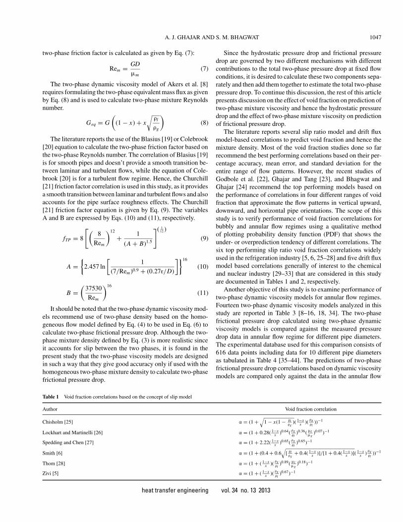
The literature reports several slip ratio model and drift fluxmodel-based correlations to predict void fraction and hence themixture density. Most of the void fraction studies done so farrecommend the best performing correlations based on their per-centage accuracy, mean error, and standard deviation for theentire range of flow patterns. However, the recent studies ofGodbole et al. [22], Ghajar and Tang [23], and Bhagwat andGhajar [24] recommend the top performing models based onthe performance of correlations in four different ranges of voidfraction that approximate the flow patterns in vertical upward,downward, and horizontal pipe orientations. The scope of thisstudy is to verify performance of void fraction correlations forbubbly and annular flow regimes using a qualitative methodof plotting probability density function (PDF) that shows theunder- or overprediction tendency of different correlations. Thesix top performing slip ratio void fraction correlations widelyused in the refrigeration industry [5, 6, 25–28] and five drift fluxmodel based correlations generally of interest to the chemicaland nuclear industry [29–33] that are considered in this studyare documented in Tables 1 and 2, respectively.

Another objective of this study is to examine performance oftwo-phase dynamic viscosity models for annular flow regimes.Fourteen two-phase dynamic viscosity models analyzed in thisstudy are reported in Table 3 [8–16, 18, 34]. The two-phasefrictional pressure drop calculated using two-phase dynamicviscosity models is compared against the measured pressuredrop data in annular flow regime for different pipe diameters.The experimental database used for this comparison consists of616 data points including data for 10 different pipe diametersas tabulated in Table 4 [35–44]. The predictions of two-phasefrictional pressure drop correlations based on dynamic viscositymodels are compared only against the data in the annular flow

Table 1 Void fraction correlations based on the concept of slip model

Author Void fraction correlation

Chisholm [25] α = (1 +√

1 − x(1 − ρlρg

)( 1−xx )(

ρgρl

))−1

Lockhart and Martinelli [26] α = (1 + 0.28( 1−xx )0.64( ρg

ρl)0.36( μl

μg)0.07)−1

Spedding and Chen [27] α = (1 + 2.22( 1−xx )0.65( ρg

ρl)0.65)−1

Smith [6] α = (1 + (0.4 + 0.6√

[ ρlρg

+ 0.4( 1−xx )]/[1 + 0.4( 1−x

x )]( 1−xx ) ρg

ρl))−1

Thom [28] α = (1 + ( 1−xx )(

ρgρl

)0.89( μlμg

)0.18)−1

Zivi [5] α = (1 + ( 1−xx )(

ρgρl

)0.67)−1



Table 2 Void fraction correlations based on the concept of drift flux model

Author Distribution parameter (Co) Drift velocity (Ugm)

Bhagwat and Ghajar [29] [ 1[1+cos θ]1.25 ](1−α)0.5 + 0.18(

UslUsl+Usg )0.1 R(0.35 sin θ + 0.54 cos θ)

√(

gD(ρl −ρg )ρl

)(1 − α)−0.5 sin θ

Where, R = ( μlμw

)−0.25

Gomez et al. [30] 1.15 1.53(gσ(ρl−ρg

ρ2l

))0.25(1 − α)0.5sinθ

Hibiki and Ishii [31] 1.2 − 0.2√

ρgρl

1.41(gσ(ρl−ρg)

ρ2l

)0.25(1 − α)1.75

Rouhani and Axelsson [32] 1 + 0.2(1 − x)(gDρ2

lG2 )0.25 1.18(gσ(

ρl −ρg

ρ2l

))0.25

1 + 0.2(1 − x)

Woldesemayat and Ghajar [33]a UsgUsl+Usg [1 + (

UslUsg )(ρg/ρl )0.1

] 2.9( gDσ(1+cos θ)(ρl −ρg )

ρ2l

)0.25(1.22 + 1.22 sin θ)PatmPsys

aThe leading constant 2.9 in the drift velocity equation carries a unit of [m0.25].

regime since all of these correlations predict data correctly inbubbly flow regime.

RESULTS AND DISCUSSION

Effect of Void Fraction on Prediction of HydrostaticPressure Drop

As mentioned earlier, the two-phase hydrostatic pressuredrop depends upon the calculation of the two-phase mixturedensity, which in turn depends on the accurate prediction ofvoid fraction. The two-phase mixture density is found to be sen-sitive to the error in prediction of void fraction. Moreover, thissensitivity of two-phase density and hence the hydrostatic pres-sure drop to the error in prediction of void fraction is different fordifferent values of void fraction, and in comparison to other pipe

orientations it is observed to magnify for vertical upward pipeorientation and large values of void fraction as shown in Fig-ure 3. In vertical upward flow, for the small range of void fraction(bubbly flow), a 10% error in prediction of void fraction virtuallydoes not affect the two-phase mixture density, whereas a 10%error in the high range of void fraction significantly alters thecalculated two-phase mixture density and hence the hydrostaticpressure drop. The influence of error in void fraction on hydro-static pressure drop may be significant for large-diameter pipeswhere the contribution of hydrostatic pressure drop to the totalpressure drop is significant compared to small-diameter pipes.

The effect of void fraction on two-phase mixture density andhence the hydrostatic pressure drop in vertical upward bubblyflow regime for two different pipe diameters is shown in Fig-ure 4. In Figures 4a and b, the error bands on hydrostatic pressuredrop component are due to ±10% error in prediction of voidfraction in bubbly flow for D = 12.5 mm and D = 44.5 mm,

Table 3 Two-phase mixture dynamic viscosity models

Number Author Expression for two-phase dynamic viscosity

1 Akers et al. [8] μm = μl

(1−x)+x√

ρl /ρg

2 Beattie and Whalley [9] μm = μl (1 − β)(1 + 2.5β) + μgβ

3 Ciccihitti et al. [10] μm = xμg + (1 − x)μl

4 Davidson et al. [11] μm = μl (1 + x( ρlρg

− 1))

5 Dukler et al. [12] μm = ρm (x(μgρg

) + (1 − x)( μlρl

))

6 Fourar and Boris [14] μm = (1 − β)μl + βμg + 2√

β(1 − β)μlμg

7 Garcia et al. [15] μm = μl ρgxρl +(1−x)ρg

8 Lin et al. [18] μm = μl μg

μg+x1.4(μl −μg )

9 McAdams et al. [13] μm = ( xμg

+ 1−xμl

)−1

10 Oliemans [34] μm = μl (1−β)+μgα

(1−β+α)

11 Awad and Muzychka [16] model 1 μm = μl2μl +μg−2(μl −μg )x2μl +μg+(μl −μg )x

12 Awad and Muzychka [16] model 2 μm = μg2μg+μl −2(μg−μl )(1−x)2μg+μl +(μg−μl )(1−x)

13 Awad and Muzychka [16] model 3 Arithmetic mean of model 1 and model 2

14 Awad and Muzychka [16] model 4 μm = 14

((3x − 1)μg + [3(1 − x) − 1]μl+√

[(3x − 1)μg + (3{1 − x} − 1)μl ]2 + 8μgμl

)



Figure 3 Effect of error in the prediction of void fraction on the estimation oftwo-phase hydrostatic pressure drop. (Color figure available online.)

respectively. However, in Figures 5a and b, the error bands onhydrostatic pressure drop component are for ±10% error in pre-diction of the void fraction in the annular flow regime for theaforementioned pipe diameters. The error bars represent actualdeviation and not the percentage error between the measuredand predicted values of hydrostatic pressure drop. It is evidentthat the error in void fraction virtually does not affect the hy-drostatic pressure drop in bubbly flow regime, whereas the errorin void fraction has a significant impact on hydrostatic pressuredrop and is pronounced for large-diameter pipes in an annularflow regime. This implies that for a fixed pipe diameter and voidfraction, a 10% error in prediction of void fraction in bubbly re-gion gives a small deviation in measured and predicted values ofhydrostatic pressure drop compared to that in the annular flowregime. Thus, while analyzing the void fraction correlations fortheir accuracy, relaxed performance criteria may be consideredacceptable for bubbly flow (low region of the void fraction)while stringent criteria may be imposed for annular flow regime(high region of the void fraction).

Performance of Void Fraction Correlations in Predictionof Two-Phase Mixture Density

Once the dependency and sensitivity of two-phase mixturedensity and hence the hydrostatic pressure drop on void fractionare established, it is important to analyze performance of differ-ent void fraction correlations available in the literature and theiraccuracy in prediction of two-phase density. The experimentaldatabase of void fraction used in this study to compare differentvoid fraction correlations is reported in Godbole et al. [22]. Thequalitative and quantitative performance of different slip ratiomodels and DFM-based correlations is presented in the follow-ing paragraphs. The qualitative performance analysis is carriedout in terms of PDF (probability density function) to get an ideaof over- or underprediction tendency of these correlations. Thequantitative performance analysis of slip ratio models and DFM-based correlations in prediction of void fraction and hence thetwo-phase mixture density for bubbly and annular flow regimesis documented in Tables 5 and 6, respectively. The quantitativeperformance analysis presented in the form of percentage erroris based upon direct comparison of the predicted values withthe measured data (296 for bubbly flow and 476 for annularflow) reported by Godbole et al. [22]. Figures 6 and 7 showthe probability density functions of different slip ratio modeland DFM-based void fraction correlations for bubbly flow,respectively. It is evident that the DFM correlations performbetter than slip ratio model-based correlations in prediction ofvoid fraction. All of the slip ratio model-based correlations withthe exception of Thom [28] tend to significantly overpredict thevoid fraction in bubbly flow regime. Among DFM correlations,Bhagwat and Ghajar [29], Gomez et al. [30], Hibiki and Ishii[31], and Rouhani and Axelsson [32] give comparable perfor-mance, while that of Woldesemayat and Ghajar [33] tends tooverpredict the data. The effect of prediction of slip ratio model-and DFM-based void fraction correlations on the two-phasemixture density in bubbly flow regime is shown in Figures 8and 9, respectively. The performance of Zivi [5] in predictionof low values of void fraction (bubbly flow) is observed to be

Table 4 Experimental data used to analyze two-phase dynamic viscosity models

Source D (mm) Number of data pointsa Void fraction range L/D Fluid combination

MacGillivray [35] 9.5 113 (R) 0.87–0.94 76 Air–waterAggour [36] 11.7 22 (R) 0.77–0.93 130 Helium–waterVijay [37] 11.7 20 (R) 0.76–0.89 130 Air–waterSujumnong [38] 11.7 45 (R) 0.79–0.93 130 Air–water

Air–glycerol + waterTang et al. [44] 12.52 32 (S), 34 (R) 0.76–0.98 100 Air–waterChiang [39] 12.7 94 (S) 0.77–0.89 205 Air–water

15.7 32 (S) 184Asali [40] 22.9 30 (S) 0.92–0.98 — Air–water

42 47 (S) Air–glycerol + waterOshinowo [41] 25.4 26 (S) 0.82–0.96 100 Air–waterNguyen [42] 44.5 81 (S) 0.81–0.98 40 Air–waterBelt et al. [43] 50 40 (S) 0.92 –0.98 170 Air–water

a(S) and (R) represent smooth and rough pipes, respectively.



Table 5 Quantitative performance of slip model based correlations in prediction of void fraction and mixture density

Void fraction Two-phase density

±10% Error bands ±20% Error bands ±20% Error bands ±30% Error bands

Correlation Bubbly Annular Bubbly Annular Bubbly Annular Bubbly Annular

Chisholm [25] 22.6 86.3 39.8 98.5 86.8 31.4 93 45.6Lockhart and Martinelli [26] 29.72 85.2 56 97.4 92.5 36.8 98 53.5Spedding and Chen [27] 34.5 81.6 58.1 97.4 93.9 36.8 97.3 52.9Smith [6] 28.7 82.4 48.3 97.8 89.2 29.1 93.9 39.6Thom [28] 3.7 63.3 6.75 95.07 93.9 10.5 98.3 17.8Zivi [5] 0 58.2 0 95.5 70.6 8.9 86.4 15.2

drastically poor and hence its PDF is not included in Figures 6and 8.

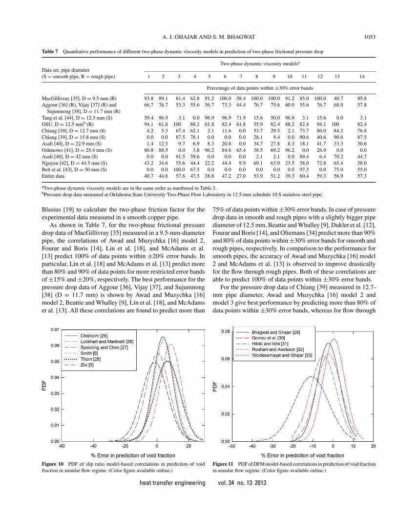
Further analysis of performance of void fraction correlationsin the annular flow regime using PDFs is as shown in Figures 10and 11. As shown in Figure 10, the slip-ratio-based correlationsof Lockhart and Martinelli [26], Smith [6], and Chisholm [25]predict majority of the data within ±20% error bands, while thecorrelation of Zivi [5] tends to overpredict the data. The perfor-mance of DFM correlations illustrated in Figure 11 shows thatthe correlations by Woldesemayat and Ghajar [33] and Bhagwatand Ghajar [29] give comparable performance, while the leastaccuracy is given by the Rouhani and Axelsson [32] correlation.In fact, the correlations of Woldesemayat and Ghajar [33] andBhagwat and Ghajar [29] predict more than 90% of data pointswithin ±10% error bands. The effect of accuracy of these slipratio model- and DFM-based correlations on two-phase mixturedensity in annular flow regime is illustrated in Figures 12 and13, respectively. Based on the PDF values and the shape anddistribution of the curves, it is clear that the DFM-based voidfraction correlations perform better than the slip ratio model-based correlations in prediction of two-phase mixture densityfor annular flow regime. In this flow regime, the correlations ofWoldesemayat and Ghajar [33] and Bhagwat and Ghajar [29]give performance superior to all other DFM-based correlationsconsidered in this study. It should be noted that the performanceof different correlations in terms of their PDF distribution isa statistical tool inclined more toward a qualitative compari-son and hence gives a qualitative guess of comparison amongdifferent void fraction correlations.

Overall, in comparison to DFM correlations the slip ratiomodel-based correlations are found to perform poorly in pre-diction of void fraction in bubbly flow regime. The maximumaccuracy is given by Lockhart and Martinelli [26] and Speddingand Chen [27] and predicts only more than 55% of data pointswithin ±20% error bands whereas the top performing DFMcorrelations such as by Bhagwat and Ghajar [29] and Rouhaniand Axelsson [32] predict more than 80% of data points withinthis performance criterion. However, it should be noted that inspite of poor performance of the slip ratio model-based voidfraction correlations in bubbly flow regime, the quantitativeperformance of both slip ratio model and DFM void fractioncorrelations is comparable in prediction of two-phase mixturedensity. This justifies that the two-phase mixture density is not astrong function of void fraction in bubbly flow regime. Althoughthese correlations predict more than 90% of two-phase mixturedensity data within ±30% error bands, for the small region ofthe void fraction (bubbly flow) ±30% error in mixture densitytranslates to ±30% error in hydrostatic pressure drop. As men-tioned earlier, the total two-phase pressure drop for nonboilingtwo-phase flow is composed of hydrostatic and frictional pres-sure drops and hence is biased to inaccuracies induced in both ofthese pressure drop components. Thus, for accurate estimationof total two-phase pressure drop it is always desired to keep theerror in two-phase mixture density and hence hydrostatic pres-sure drop and frictional pressure drop to a minimum. From thisaccuracy standpoint, further performance analysis of drift fluxmodel-based correlations for bubbly flow regimes shows that thecorrelation of Woldesemayat and Ghajar [33] can predict only

Table 6 Quantitative performance of DFM correlations in prediction of void fraction and mixture density

Void fraction Two-phase density

±10% Error bands ±20% Error bands ±20% Error bands ±30% Error bands

Correlation Bubbly Annular Bubbly Annular Bubbly Annular Bubbly Annular

Bhagwat and Ghajar [29] 49.6 95.2 80 99.5 99.3 41.5 99.6 55.8Gomez et al. [30] 46.2 85.2 74.3 100 98.6 38.7 99.3 54.6Hibiki and Ishii [31] 37.8 74.9 66.5 100 95.2 38.8 97.9 49.8Rouhani and Axelsson [32] 53.3 44.1 81 86.7 99.3 19.9 99.6 25.4Woldesemayat and Ghajar [33] 19.2 93.14 33.1 99.8 98.3 40.8 99.6 64.2



Figure 4 Contribution of hydrostatic and frictional component of pressuredrop to the total two-phase pressure drop for low region of void fraction.

43.6% and 9.8% of data points of two-phase mixture densitywithin ±10% and ±5% error bands, respectively. However, thecorrelation of Bhagwat and Ghajar [29] can predict 98.6% and90.5% of two-phase mixture density data points within ±10%and ±5% error bands, respectively.

For the annular flow regime, although the majority of correla-tions predict more than 95% of void fraction data within ±20%error bands, these correlations perform poorly in prediction of

Figure 5 Contribution of hydrostatic and frictional component of pressuredrop to the total two-phase pressure drop for high region of void fraction.

two-phase mixture density. The best accuracy is displayed byWoldesemayat and Ghajar [33] by predicting 64.2% of two-phase mixture density data points within ±30% error bandscriterion.

Overall, due to superior performance of the DFM void frac-tion correlations it is recommended to use the correlation ofBhagwat and Ghajar [29] for the low region of void frac-tion (bubbly flow), while for the high region of void fraction



Figure 6 PDF of slip ratio model-based correlations in prediction of voidfraction in bubbly flow regime. (Color figure available online.)

(annular flow), the correlation of Woldesemayat and Ghajar[33] may be preferred.

Effect of Two-Phase Dynamic Viscosity Models on Predictionof Two-Phase Frictional Pressure Drop

The two-phase frictional pressure drop correlations basedon two-phase dynamic viscosity models predict the measuredfrictional pressure drop correctly for bubbly flow regime andhence their performance for bubbly flow is not reported in thisstudy. However, the performance of these models in predictingfrictional pressure drop data in annular flow regime needs to beinvestigated. The following section deals with the performanceanalysis of two-phase dynamic viscosity models in predictionof two-phase frictional pressure drop. Based on the overall

Figure 7 PDF of DFM-based correlations in prediction of void fraction inbubbly flow regime. (Color figure available online.)

Figure 8 PDF of slip ratio model-based void fraction correlations in predictionof two-phase mixture density for bubbly flow (low region of void fraction).(Color figure available online.)

performance of two-phase dynamic viscosity models it isdecided to analyze their accuracy based on the percentage ofdata predicted within ±30% error bands as shown in Table 7.A similar type of performance criteria had been used by Awadand Muzychka [16] and Dalkilic et al. [45]. Dalkilic et al. [45]carried out a similar type of study to investigate the differenttwo-phase viscosity models available in the literature and com-pared their performance against the experimental data of R134refrigerant undergoing condensation in vertical downwardpipe. They found that the correlations of Fourar and Boris [14]and Davidson et al. [11] showed consistent discrepancy withthe measured data, whereas the correlations of Dukler et al.[12], Lin et al. [18], Garcia et al. [15], and McAdams et al.[13] predicted the measured two-phase friction factor within±30% error bands. They used the friction factor equation of

Figure 9 PDF of DFM-based void fraction correlations in prediction of two-phase mixture density for bubbly flow (low region of void fraction). (Colorfigure available online.)



Table 7 Quantitative performance of different two-phase dynamic viscosity models in prediction of two-phase frictional pressure drop

Two-phase dynamic viscosity modelsa

Data set, pipe diameter(S = smooth pipe, R = rough pipe) 1 2 3 4 5 6 7 8 9 10 11 12 13 14

Percentage of data points within ±30% error bands

MacGillivray [35], D = 9.5 mm (R) 93.8 99.1 81.4 62.8 91.2 100.0 58.4 100.0 100.0 91.2 85.0 100.0 40.7 85.8Aggour [36] (R), Vijay [37] (R) and

Sujumnong [38], D = 11.7 mm (R)66.7 76.7 53.3 55.6 56.7 73.3 44.4 76.7 75.6 60.0 55.6 76.7 68.9 57.8

Tang et al. [44], D = 12.5 mm (S) 59.4 96.9 3.1 0.0 96.9 96.9 71.9 15.6 50.0 96.9 3.1 15.6 0.0 3.1OSU, D = 12.5 mmb (R) 94.1 61.8 100 88.2 61.8 82.4 61.8 55.9 82.4 88.2 82.4 94.1 100 82.4Chiang [39], D = 12.7 mm (S) 4.2 5.3 67.4 62.1 2.1 11.6 0.0 53.7 29.5 2.1 73.7 80.0 84.2 76.8Chiang [39], D = 15.8 mm (S) 0.0 0.0 87.5 78.1 0.0 0.0 0.0 28.1 9.4 0.0 90.6 40.6 90.6 87.5Asali [40], D = 22.9 mm (S) 1.4 12.5 9.7 6.9 8.3 20.8 0.0 34.7 27.8 8.3 18.1 41.7 33.3 30.6Oshinowo [41], D = 25.4 mm (S) 80.8 88.5 0.0 3.8 96.2 84.6 65.4 38.5 69.2 96.2 0.0 26.9 0.0 0.0Asali [40], D = 42 mm (S) 0.0 0.0 91.5 59.6 0.0 0.0 0.0 2.1 2.1 0.0 89.4 6.4 70.2 44.7Nguyen [42], D = 44.5 mm (S) 43.2 34.6 55.6 44.4 22.2 44.4 9.9 69.1 63.0 23.5 58.0 72.8 65.4 58.0Belt et al. [43], D = 50 mm (S) 0.0 0.0 100.0 67.5 0.0 0.0 0.0 0.0 0.0 0.0 97.5 0.0 75.0 55.0Entire data 40.7 44.6 57.6 47.5 38.8 47.2 27.0 53.9 51.2 39.3 60.4 59.3 56.9 57.3

aTwo-phase dynamic viscosity models are in the same order as numbered in Table 3.bPressure drop data measured at Oklahoma State University Two-Phase Flow Laboratory in 12.5-mm schedule 10 S stainless-steel pipe.

Blasius [19] to calculate the two-phase friction factor for theexperimental data measured in a smooth copper pipe.

As shown in Table 7, for the two-phase frictional pressuredrop data of MacGillivray [35] measured in a 9.5-mm-diameterpipe, the correlations of Awad and Muzychka [16] model 2,Fourar and Boris [14], Lin et al. [18], and McAdams et al.[13] predict 100% of data points within ±20% error bands. Inparticular, Lin et al. [18] and McAdams et al. [13] predict morethan 80% and 90% of data points for more restricted error bandsof ±15% and ±20%, respectively. The best performance for thepressure drop data of Aggour [36], Vijay [37], and Sujumnong[38] (D = 11.7 mm) is shown by Awad and Muzychka [16]model 2, Beattie and Whalley [9], Lin et al. [18], and McAdamset al. [13]. All these correlations are found to predict more than

Figure 10 PDF of slip ratio model-based correlations in prediction of voidfraction in annular flow regime. (Color figure available online.)

75% of data points within ±30% error bands. In case of pressuredrop data in smooth and rough pipes with a slightly bigger pipediameter of 12.5 mm, Beattie and Whalley [9], Dukler et al. [12],Fourar and Boris [14], and Oliemans [34] predict more than 90%and 80% of data points within ±30% error bands for smooth andrough pipes, respectively. In comparison to the performance forsmooth pipes, the accuracy of Awad and Muzychka [16] model2 and McAdams et al. [13] is observed to improve drasticallyfor the flow through rough pipes. Both of these correlations areable to predict 100% of data points within ±30% error bands.

For the pressure drop data of Chiang [39] measured in 12.7-mm pipe diameter, Awad and Muzychka [16] model 2 andmodel 3 give best performance by predicting more than 80% ofdata points within ±30% error bands, whereas for flow through

Figure 11 PDF of DFM model-based correlations in prediction of void fractionin annular flow regime. (Color figure available online.)



Figure 12 PDF of slip ratio model-based void fraction correlations in predic-tion of two-phase mixture density for annular flow (high region of void fraction).(Color figure available online.)

15.8-mm-diameter pipe, Awad and Muzychka [16] model 1 andmodel 3 predict more than 90% of data points within ±30% er-ror bands. For the pressure drop data of Oshinowo [41] througha D = 25.4 mm smooth pipe, the best performance is given byDukler et al. [12] and Oliemans [34] by predicting more than95% of data points within ±30% error bands. This is followedby the performances of Beattie and Whalley [9] and Fourar andBoris [14] that predict more than 85% and 80% of data pointsfor error criteria similar to that already mentioned. The pressuredrop data of Asali [40], Nguyen [42], and Belt et al. [43] is forlarge pipe diameters compared to other experimental data usedin this study. The correlations of Ciccihitti et al. [10] and Awadand Muzychka [16] model 1 predict 91% and 100% of data and89.4% and 97.5% of data within ±30% error bands for D =42 mm and D = 50 mm, respectively. Although, the data of

Figure 13 PDF of DFM based void fraction correlations in prediction of two-phase mixture density for annular flow (high region of void fraction). (Colorfigure available online.)

Nguyen [42] are for a pipe diameter similar to that of Asali [40],the correlations of Ciccihitti et al. [10] and Awad and Muzy-chka [16] model 1 can predict only 56% and 58% of data pointswithin ±30% error bands. A plausible reason for the inability ofthese correlations to predict the data of Nguyen [42] is that thisexperimental frictional pressure drop data is collected at a pipeaxial location of L/D = 40. Literature review shows that pres-sure drop data collected for small L/D ratios may not representthe actual pressure gradient, since for this L/D = 40 pipe axialdistance, the two phases may not be completely aligned witheach other and their distribution with respect to each other andhence the pressure gradient may change at downstream of inlet.More details about the change in pressure gradient with respectto the nondimensional pipe axial length (L/D) are reported byWolf et al. [46].

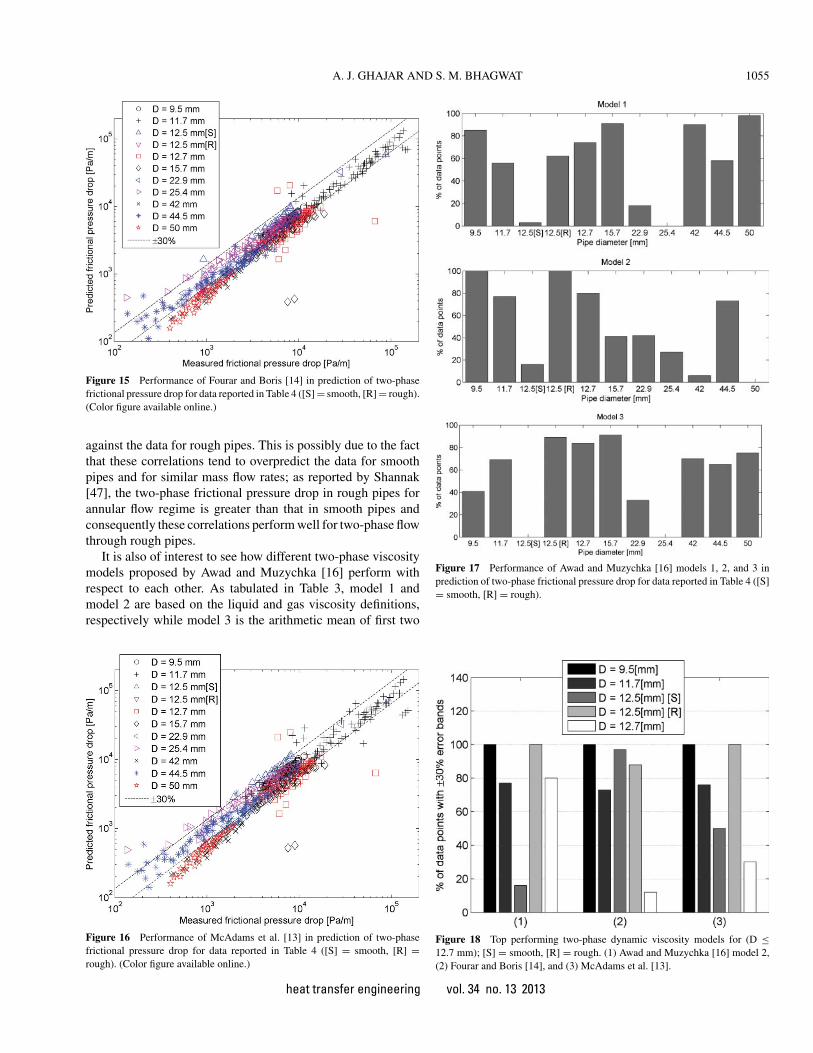
Overall, performance analysis of two-phase dynamic viscos-ity models shows that they underpredict the pressure drop datafor large pipe diameters of Asali [40] and Belt et al. [43]. Theprobable reason for the correlations to underpredict the largepipe diameters is that, in addition to friction at the pipe wall,friction at the gas–liquid interface contributes significantly tothe total frictional pressure drop and the two-phase viscositymodels do not account for the increase in interfacial frictionwith increase in the pipe diameter. In addition to the correlationof Awad and Muzychka [16] model 1, the correlations of Cicci-hitti et al. [10] and Davidson et al. [11] that predict the frictionalpressure drop for large diameter with good accuracy essentiallytend to overpredict the frictional pressure drop for comparativelysmaller pipe diameters at given flow conditions and hence prob-ably account for the added effect of interfacial friction in largediameter pipes. The overprediction tendency of Ciccihitti et al.[10] and comparative underprediction trend of Fourar and Boris[14] and McAdams et al. [13] are clear from the general shift inthe predicted data shown in Figures 14–16, respectively.

It should be noted that in comparison to the flow throughsmooth pipes, the majority of the correlations perform better

Figure 14 Performance of Ciccihitti et al. [10] in prediction of two-phasefrictional pressure drop for data reported in Table 4 ([S] = smooth, [R] =rough). (Color figure available online.)



Figure 15 Performance of Fourar and Boris [14] in prediction of two-phasefrictional pressure drop for data reported in Table 4 ([S] = smooth, [R] = rough).(Color figure available online.)

against the data for rough pipes. This is possibly due to the factthat these correlations tend to overpredict the data for smoothpipes and for similar mass flow rates; as reported by Shannak[47], the two-phase frictional pressure drop in rough pipes forannular flow regime is greater than that in smooth pipes andconsequently these correlations perform well for two-phase flowthrough rough pipes.

It is also of interest to see how different two-phase viscositymodels proposed by Awad and Muzychka [16] perform withrespect to each other. As tabulated in Table 3, model 1 andmodel 2 are based on the liquid and gas viscosity definitions,respectively while model 3 is the arithmetic mean of first two

Figure 16 Performance of McAdams et al. [13] in prediction of two-phasefrictional pressure drop for data reported in Table 4 ([S] = smooth, [R] =rough). (Color figure available online.)

Figure 17 Performance of Awad and Muzychka [16] models 1, 2, and 3 inprediction of two-phase frictional pressure drop for data reported in Table 4 ([S]= smooth, [R] = rough).

Figure 18 Top performing two-phase dynamic viscosity models for (D ≤12.7 mm); [S] = smooth, [R] = rough. (1) Awad and Muzychka [16] model 2,(2) Fourar and Boris [14], and (3) McAdams et al. [13].



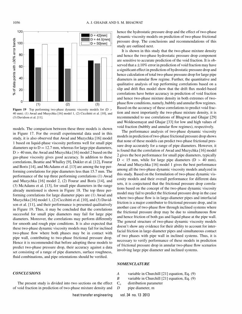
Figure 19 Top performing two-phase dynamic viscosity models for (D >

40 mm). (1) Awad and Muzychka [16] model 1, (2) Ciccihitti et al. [10], and(3) Davidson et al. [11].

models. The comparison between these three models is shownin Figure 17. For the overall experimental data used in thisstudy, it is also observed that Awad and Muzychka [16] model1 based on liquid-phase viscosity performs well for small pipediameters up to D = 12.7 mm, whereas for large pipe diameters,D > 40 mm, the Awad and Muzychka [16] model 2 based on thegas-phase viscosity gives good accuracy. In addition to thesecorrelations, Beattie and Whalley [9], Dukler et al. [12], Fourarand Boris [14], and McAdams et al. [13] are among the top per-forming correlations for pipe diameters less than 15.7 mm. Theperformance of the top three performing correlations (1) Awadand Muzychka [16] model 2, (2) Fourar and Boris [14], and(3) McAdams et al. [13], for small pipe diameters in the rangealready mentioned is shown in Figure 18. The top three per-forming correlations for large diameter pipes are (1) Awad andMuzychka [16] model 1, (2) Ciccihitti et al. [10], and (3) David-son et al. [11], and their performance is presented qualitativelyin Figure 19. Thus, it may be concluded that the correlationssuccessful for small pipe diameters may fail for large pipediameters. Moreover, the correlations may perform differentlyfor smooth and rough pipe conditions. It is also expected thatthese two-phase dynamic viscosity models may fail for inclinedtwo-phase flow where both phases may be in contact withpipe wall, contributing to two-phase frictional pressure drop.Hence it is recommended that before adopting these models topredict two-phase pressure drop, their accuracy against a dataset consisting of a range of pipe diameters, surface roughness,fluid combinations, and pipe orientations should be verified.

CONCLUSIONS

The present study is divided into two sections on the effectof void fraction in prediction of two-phase mixture density and

hence the hydrostatic pressure drop and the effect of two-phasedynamic viscosity models on prediction of two-phase frictionalpressure drop. The conclusions and recommendations of thisstudy are outlined next.

It is shown in this study that the two-phase mixture densityand hence the two-phase hydrostatic pressure drop componentare sensitive to accurate prediction of the void fraction. It is ob-served that a ±10% error in prediction of void fraction may havea significant effect in prediction of hydrostatic pressure drop andhence calculation of total two-phase pressure drop for large pipediameters in annular flow regime. Further, the quantitative andqualitative analysis of top performing correlations based on aslip and drift flux model show that the drift flux model-basedcorrelations have better accuracy in prediction of void fractionand hence two-phase mixture density in both extremes of two-phase flow conditions, namely, bubbly and annular flow regimes.Based on the accuracy of these correlations to predict void frac-tion and most importantly the two-phase mixture density, it isrecommended to use correlations of Bhagwat and Ghajar [29]and Woldesemayat and Ghajar [33] for low and high values ofvoid fraction (bubbly and annular flow regimes), respectively.

The performance analysis of two-phase dynamic viscositymodels in prediction of two-phase frictional pressure drop showsthat none of these models can predict two-phase frictional pres-sure drop accurately for a range of pipe diameters. However, itis found that the correlation of Awad and Muzychka [16] model2 gives the best performance for small pipe diameters, typicallyD < 15 mm, while for large pipe diameters (D > 40 mm),Awad and Muzychka [16] model 1 gives the best performanceamong all the two-phase dynamic viscosity models analyzed inthis study. Based on the formulation of two-phase dynamic vis-cosity models and their overall performance for different datasets, it is conjectured that the frictional pressure drop correla-tions based on the concept of the two-phase dynamic viscositymodel may fail to predict the frictional pressure drop in the casewhere two-phase flow is in large-diameter pipes and interfacialfriction is a major contributor to frictional pressure drop, and inanother case of two-phase flow through inclined systems wherethe frictional pressure drop may be due to simultaneous flowand hence friction of both gas and liquid phase at the pipe wall.The general structure of two-phase dynamic viscosity modelsdoesn’t show any evidence for their ability to account for inter-facial friction in large-diameter pipes and simultaneous contactof two phases with pipe wall in inclined systems. Thus, it isnecessary to verify performance of these models in predictionof frictional pressure drop in annular two-phase flow scenariosinvolving large pipe diameter and inclined systems.

NOMENCLATURE

A variable in Churchill [21] equation, Eq. (9)B variable in Churchill [21] equation, Eq. (9)Co distribution parameterD pipe diameter, m



DFM drift flux modelf friction factorg acceleration due to gravity, m/s2

G two-phase mixture mass flux, (G = Gl + Gg), kg/m2-sL pipe length, mP pressure, PaPDF probability density functionRe Reynolds numberS slip ratioU phase velocity, m/sUgm drift velocity, m/sx quality

Greek Symbols

α void fractionβ gas volumetric flow fractionρ phase density, kg/m3

μ phase dynamic viscosity, Pa-sσ surface tension, N/mε surface roughness, mθ pipe orientation (inclination angle), degrees

Subscripts

a accelerationatm atmosphericeq equivalentf frictiong gas phaseh hydrostatici pipe inletl liquid phasem mixtureo pipe outlets superficialsys systemt totalTP two phasew water

REFERENCES

[1] Farzad, M., and O’Neal, D. L., The Effect of Void FractionModel on Estimation of Air Conditioner System Perfor-mance Variables Under a Range of Refrigerant ChargingConditions, International Journal of Refrigeration, vol. 17,no. 2, pp. 85–93, 1994.

[2] Ma, X., Ding, G., Zhang, P., Han, W., Kasahara, S., andYamaguchi, T., Experimental Validation of Void FractionModels for R410 Air Conditioners, International Journalof Refrigeration, vol. 32, pp. 780–790, 2009.

[3] Barcozy, C. J., A Systematic Correlation for Two PhasePressure Drop, Chemical Engineering Progress, vol. 62,no. 44, pp. 232–249, 1966.

[4] Hughmark, G. A., Holdup in Gas Liquid Flow, ChemicalEngineering Progress, vol. 58, pp. 62–65, 1962.

[5] Zivi, S. M., Estimation of Steady State Steam Void Fractionby Means of the Principle of Minimum Entropy Produc-tion, Trans. ASME, Journal of Heat Transfer, vol. 86, pp.247–252, 1964.

[6] Smith, S. L., Void Fraction in Two Phase Flow: A Correla-tion Based Upon an Equal Velocity Head Model, Instituteof Mechanical Engineers, vol. 184, no. 36, pp. 647–664,1969.

[7] Permoli, A., Francesco, D., and Prima, A., An EmpiricalCorrelation for Evaluating Two Phase Mixture DensityUnder Adiabatic Conditions, European Two Phase FlowGroup Meeting, Milan, Italy, 1970.

[8] Akers, W. W., Deans, A., and Crossee, O. K., CondensingHeat Transfer Within Horizontal Tubes, Chemical Engi-neering Progress, vol. 55, pp. 171–176, 1959.

[9] Beattie, D. R. H., and Whalley, P. B., A Simple Two-Phase Frictional Pressure Drop Calculation Method, Inter-national Journal of Multiphase Flow: Brief Communica-tion, vol. 8, pp. 83–87, 1982.

[10] Ciccihitti, A., Lombardi, C., Silvestri, M., Soldaini, R., andZavatarelli, G., Two-Phase Cooling Experiments: PressureDrop, Heat Transfer and Burn Out Measurments, EnergiaNuclear, vol. 7, pp. 407–429, 1960.

[11] Davidson, W. F., Hardie, P. H., Humphreys, C. G. R., Mark-son, A. A., Mumford, A. R., and Ravese, T., Studies of HeatTransmission Through Boiler Tubing at Pressures From500–3300 lbs, Trans. ASME, vol. 65, no. 6, pp. 553–591,1943.

[12] Dukler, A. E., Wicks, M., and Cleveland, R. G., FrictionalPressure Drop in Two Phase Flow: Part A and B, AIChE,vol. 10, pp. 38–51, 1964.

[13] McAdams, W. H., Woods, W. K., and Heroman, L. V., Va-porization Inside Horizontal Tubes—II. Benzene Oil Mix-tures, Trans. ASME, vol. 64, pp. 193–200, 1942.

[14] Fourar, M., and Boris, S., Experimental Study of Air WaterTwo Phase Flow Through a Fracture, International Journalof Multiphase Flow, vol. 4, pp. 621–637, 1995.

[15] Garcia, F., Garcia, R., Padrino, J. C., Mata, C., Trallero, J.L., and Joseph, D. D., Power Law Composite Power LawFriction Factor Correlations for Laminar Turbulent GasLiquid Flow in Horizontal Pipe Lines, International Jour-nal of Multiphase Flow, vol. 29, no. 10, pp. 1605–1624,2003.

[16] Awad, M. M., and Muzychka, Y. S., Effective PropertyModels for Homogeneous Two-Phase Flows, Experimen-tal Thermal and Fluid Science, vol. 33, pp. 106–113, 2008.

[17] Einstein, A., A New Determinaiton of Molecular Dimen-sions, Annals of Physics, vol. 19, pp. 289–306, 1906.

[18] Lin, S., Kwok, C. C. K., Li, R. Y., Chen, Z. H., and Chen,Z. Y., Local Frictional Pressure Drop During Vaporization



of R12 Through Capillary Tubes, International Journal ofMultiphase Flow, vol. 17, pp. 95–102, 1991.

[19] Blasius, H., Das Anhlichkeitsgesetz bei Reibungsvorgan-gen in Flussikeiten, Gebiete Ingenieurw, vol. 131, pp.1–41, 1913.

[20] Colebrook, C. F., Turbulent Flow in Pipes, With ParticularReference to the Transition between the Smooth and RoughPipe Laws, Journal of Institute of Civil Engineering, vol.11, pp. 1938–1939, 1939.

[21] Churchill, S. W., Friction Factor Equation Spans All Fluid-Flow Regimes, Chemical Engineering, vol. 7, pp. 91–92,1977.

[22] Godbole, P. V., Tang, C. C., and Ghajar, A. J., Comparisonof Void Fraction Correlations for Different Flow Patternsin Upward Vertical Two Phase Flow, Heat Transfer Engi-neering, vol. 32, no. 10, pp. 843–860, 2011.

[23] Ghajar, A. J., and Tang, C. C., Void Fraction and FlowPatterns of Two-Phase Flow in Upward and DownwardVertical and Horizontal Pipes, Advances in MultiphaseFlow and Heat Transfer, vol. 4, Chapter 7, pp. 175–201,2012.

[24] Bhagwat, S. M., and Ghajar, A. J., Similarities and Differ-ences in the Flow Patterns and Void Fraction in VerticalUpward and Downward Two Phase Flow, ExperimentalThermal and Fluid Sciences, vol. 39, pp. 213–227, 2012.

[25] Chisholm, D., Pressure Gradients Due to Friction DuringFlow of Evaporating Two Phase Mixtures in Smooth Tubesand Channels, International Journal of Heat and MassTransfer, vol. 16, pp. 347–358, 1973.

[26] Lockhart, R. W., and Martinelli, R. C., Proposed Correla-tion Of Data for Isothermal Two Phase, Two ComponentFlow in Pipes, Chemical Engineering Progress, vol. 45,pp. 39–48, 1949.

[27] Spedding, P. L., and Chen, J. J., Holdup in Two PhaseFlow, International Journal of Multiphase Flow, vol. 10,pp. 307–339, 1984.

[28] Thom, J. R. S., Prediction of Pressure Drop During ForcedCirculation Boiling of Water, International Journal of Heatand Mass Transfer, vol. 7, pp. 709–724, 1964.

[29] Bhagwat, S. M., and Ghajar, A. J., Flow Pattern andPipe Orientation Independent Semi-Empirical Void Frac-tion Correlation for a Gas–liquid Two-Phase Flow Basedon the Concept of Drift Flux Model, Proc. of ASME2012 Summer Heat Transfer Conference, Puerto Rico,2012.

[30] Gomez, L. E., Shoham, O., Schmidt, Z., Choshki, R. N.,and Northug, T., Unified Mechanistic Model for SteadyState Two Phase Flow: Horizontal to Upward VerticalFlow, Society of Petrolium Enginners Journal, vol. 5, pp.339–350, 2000.

[31] Hibiki, T., and Ishii, M., One-Dimensional Drift FluxModel and Constituive Equations for Relative Motion Be-tween Phases in Various Two-Phase Flow Regimes, Inter-national Journal of Heat and Mass Transfer, vol. 46, pp.4935–4948, 2003.

[32] Rouhani, S. Z., and Axelsson, E., Calculation of Void Vol-ume Fraction in the Subcooled and Quality Boiling Re-gions, International Journal of Heat and Mass Transfer,vol. 13, pp. 383–393, 1970.

[33] Woldesemayat, M. A., and Ghajar, A. J., Comparision ofVoid Fraction Correlations for Different Flow Patterns inHorizontal and Upward Inclined Pipes, International Jour-nal of Multiphase Flow, vol. 33, pp. 347–370, 2007.

[34] Oliemans, R., Two Phase Flow in Gas TransmissionPipelines, Petroleum Division ASME Meeting, Paper 76,Pet-25, Mexico, 1976.

[35] MacGillivray, R. M., Gravity and Gas Density Effectson Annular Flow Average Film Thickness and FrictionalPressure Drop, M.S. Thesis, University of Saskatchewan,2004.

[36] Aggour, M. A., Hydrodynamics and Heat Transfer in Two-Phase Two-Component Flow, Ph.D. Thesis, University ofManitoba, 1978.

[37] Vijay, M. M., A Study of Heat Transfer in Two-PhaseTwo-Component Flow in a Vertical Tube, Ph.D. Thesis,University of Manitoba, 1978.

[38] Sujumnong, M., Heat Transfer, Pressure Drop and VoidFraction in Two Phase Two Component Flow in VerticalTube, Ph.D. Thesis, University of Manitoba, 1997.

[39] Chiang, R., Study of Liquid Entrainment Rates in AnnularTwo Phase Flow Through Smooth and Rifled Tubes, Ph.D.Thesis, Lehigh University, 1986.

[40] Asali, J. C., Entrainment in Vertical Gas–Liquid AnnularFlow, Ph.D. Thesis, University of Illinois Urbana Cham-paign, 1984.

[41] Oshinowo, O., Two Phase Flow in a Vertical Tube Coil,Ph.D. Thesis, University of Toronto, 1971.

[42] Nguyen, V. T., Two Phase Gas–Liquid Cocurrent Flow: AnInvestigation of Hold Up, Pressure Drop and Flow Patternin a Pipe at Various Inclinations, Ph.D. Thesis, Universityof Auckland, 1975.

[43] Belt, R. J., Van’t Westende, J. M. C., and Portela, L. M.,Prediction of the interfacial Shear Stress in Vertical Annu-lar Flow, International Journal of Multiphase Flow, vol.35, pp. 689–697, 2009.

[44] Tang, C. C., Tiwari, S., and Ghajar, A. J., Effect of VoidFraction on Pressure Drop in Upward Vertical Two PhaseGas–liquid Pipe Flow, ASME Journal of Gas Turbines andPower, vol. 135, pp. 022901-1–022901-7, 2013.

[45] Dalkilic, A. S., Kurekci, N. A., and Wongwises, S., Ef-fect of Void Fraction and Friction Factor Models on thePrediction of Pressure Drop of R-134a During DownwardCondensation in a Vertical Tube, Heat and Mass Transfer,vol. 48, no. 1, p. 2012.

[46] Wolf, A., Jayanti, S., and Hewitt, G. F., Flow Developmentin Vertical Annular Flow, Chemical Engineering Science,vol. 56, pp. 3221–3235, 2001.

[47] Shannak, B. A., Frictional Pressure Drop of Gas LiquidTwo-Phase Flow in Pipes, Nuclear Engineering and De-sign, vol. 238, pp. 3277–3284, 2008.



Afshin J. Ghajar is a Regents Professor, John Bram-mer Endowed Professor, and Director of GraduateStudies in the School of Mechanical and AerospaceEngineering at Oklahoma State University, Stillwa-ter, and a Honorary Professor of Xi’an Jiaotong Uni-versity, Xi’an, China. He received his B.S., M.S., andPh.D., all in mechanical engineering, from OklahomaState University. His expertise is in experimental heattransfer/fluid mechanics and development of practi-cal engineering correlations. He has been a summer

research fellow at Wright Patterson AFB (Dayton, OH) and Dow ChemicalCompany (Freeport, TX). He and his co-workers have published more than200 reviewed research papers and book chapters. He has delivered numerouskeynote and invited lectures at major technical conferences and institutions. Hehas received several outstanding teaching/service awards. Dr. Ghajar is a fellowof the American Society of Mechanical Engineers (ASME), Heat Transfer Se-ries editor for Taylor & Francis/CRC Press, and editor-in-chief of Heat TransferEngineering. He is also the co-author of the fourth edition of Cengel and Gha-jar, Heat and Mass Transfer—Fundamentals and Applications, McGraw-Hill,February 2010.

Swanand M. Bhagwat is currently a Ph.D. candidateat the School of Mechanical and Aerospace Engineer-ing, Oklahoma State University, Stillwater. He ob-tained his M.S. degree in Mechanical and AerospaceEngineering from Oklahoma State University in 2011and has worked on void fraction, two-phase pressuredrop, and nonboiling heat transfer in vertical down-ward two-phase flow. He received his bachelor’s de-gree in mechanical engineering in 2008 from Amra-vati University, India. His research interests are in the

general areas of two-phase flow, heat transfer, and thermodynamics.


effect of void fraction and two-phase dynamic viscosity

Documents