Dynamic Article LinksC<Soft Matter

Cite this: Soft Matter, 2012, 8, 5140

www.rsc.org/softmatter PAPER

Publ

ishe

d on

23

Mar

ch 2

012.

Dow

nloa

ded

by U

nive

rsity

of

Wes

tern

Ont

ario

on

28/1

0/20

14 0

8:50

:19.

View Article Online / Journal Homepage / Table of Contents for this issue

Effect of solvent quality on the polymer adsorption from bulk solution ontoplanar surfaces†

Per Linse

Received 11th January 2012, Accepted 5th March 2012

DOI: 10.1039/c2sm25074h

Adsorption of uncharged homopolymers in good and theta solvents onto planar surfaces at various

chain flexibility and polymer–surface attraction strengths was investigated by using a coarse-grained

bead–spring polymer model and simulation techniques. Equilibrium properties of the interfacial

systems were obtained from Monte Carlo simulations by monitoring the bead and polymer density

profiles, the number of adsorbed beads and polymers, the components of the radius of gyration

perpendicular and parallel to the surface as well as tail, loop, and train characteristics. The adsorption

process starting with a polymer-free zone adjacent to the surface was examined by Brownian dynamic

simulations. At equilibrium, the adsorbed amount increased upon increasing chain stiffness and in

poorer solvent conditions, and the structural characteristics depended also on the chain stiffness and

solvent condition. The initial adsorption was diffusion controlled, but soon it became governed by the

probability of a polymer to be captured by the surface attraction. Flexible polymers became flattened

after attaching, but their final relaxation mechanism involved an increase in perpendicular extension.

There were fewer adsorbed beads and longer tails, which was driven by the surface pressure originating

from the surrounding adsorbed polymers. This structural rearrangement became more prominent in

poorer solvent conditions. Finally, the integration time, which denotes the adsorption time for

adsorbed polymers to become fully integrated into the adsorbed layer, and the residence times of

integrated polymers were analyzed. In particular, the latter became longer with increasing chain

stiffness and shorter in poorer solvent conditions.

1 Introduction

Polymers in solution may adsorb onto surfaces if the effective

polymer–surface attraction exceeds the conformational entropy

loss of the polymer upon adsorption.1 The effective attraction

depends both on the direct polymer–surface and solvent–surface

interactions as well as on the polymer–solvent interaction.

Generally, poor solvent conditions promote adsorption.

The adsorption of polymers onto surfaces, whether desired or

not, has huge implications in many areas of research. Moreover,

understanding and controlling such processes is of great impor-

tance and is essential in many different technological aspects

ranging from the paper industry and paint formulation to

pharmaceutical applications,2 biophysics,3–5 and nanocomposite

materials.6

The adsorption of polymers onto surfaces is largely governed

by the prevailing conditions under which the polymer, solvent,

Physical Chemistry, Department of Chemistry, Lund University, P.O. Box124, S-221 00 Lund, Sweden

† Electronic supplementary information (ESI) available: Graphicalinformation displaying in more detail the adsorption process withflexible and rod-like polymers at the two solvent conditions areavailable. See DOI: 10.1039/c2sm25074h

5140 | Soft Matter, 2012, 8, 5140–5150

and surface interact. The equilibrium adsorbed layer in terms of

surface coverage and layer thickness is often of interest from

a technical point of view, where a surface is physically or

mechanically modified to meet specific requirements. Due to the

immense number of applications for polymer adsorption, there

has historically been a large interest in characterizing layers of

adsorbed polymers.7–11 However, often kinetics is so slow that

true equilibrium of the adsorbed polymers never is achieved

during realistic time scales. Resolving the different time scales

involved during the entire adsorption process, from diffusional

transport to a surface followed by subsequent attachment and

spreading on it, thus remains a significant task and a large

challenge within the field.

A number of different theoretical methods have been

employed to study the adsorption of uncharged polymers onto

uncharged surfaces from bulk solution. Such adsorption profiles

near adsorbing surfaces have been characterized by using mean-

field approaches12,13 as well as by using various simulation

techniques.14–17 The dynamics of polymer adsorption has also

been studied using dynamic mean-field schemes,18 as well as

dynamic Monte-Carlo,19–25 molecular dynamics,26–30 and Brow-

nian dynamics31,32 techniques. Some of the dynamic studies were

conducted on single polymers at a surface,22,25,31 while others

This journal is ª The Royal Society of Chemistry 2012

Publ

ishe

d on

23

Mar

ch 2

012.

Dow

nloa

ded

by U

nive

rsity

of

Wes

tern

Ont

ario

on

28/1

0/20

14 0

8:50

:19.

View Article Online

were comprised of adsorption from solutions ranging from semi-

dilute conditions20,19,21,23,24,30,32 to polymer melts.26–29 Various

static and dynamic properties of polymer adsorption have been

examined as a function of strength of the polymer–surface

interaction,14,17,21,23,31 and only a few have been conducted on

polymer models with varying intrinsic stiffness.14,16,31 Further-

more, some attention has been given to diffusion and exchange in

an adsorbed layer.21,26,27,23,33

In a previous work,34 adsorption of flexible polymers in a good

solvent onto a planar and solid surface for different polymer

flexibility and surface attraction was examined. Both equilibrium

structure and adsorption dynamics starting from a polymer-free

zone adjacent to the surface were examined. In this study, we

extend these simulation studies to comprise adsorption from

a theta solvent using both Monte Carlo and Brownian dynamics

techniques. Beside an increase in the adsorbed amount, other

equilibrium and dynamical properties were found to depend on

the solvent quality.

2 Model

The adsorption of polymers from solution onto a planar surface

is studied using a simple coarse-grained model; basically the same

model as previously described is used.31–34 The solution contains

Np polymers and each polymer is represented by a sequence ofNb

spherical beads connected via harmonic potentials. The total

number of beads in the system N is thus given by N ¼ NpNb. The

polymers are confined in a rectangular simulation box with the

box lengths Lx, Ly, and Lz. At z ¼ �(Lz/2) we have adsorbing

surfaces, whereas periodic boundary conditions are applied in

the x- and y-directions. The length of the box edges are Lx¼ Ly¼200 �A and Lz ¼ 240 �A. Our focus is on structures and events

occurring near the surfaces. Therefore, a coordinate system with

a z-axis starting at z ¼ Lz/2 and directed into the solution is

adopted, and averages over both equivalent surfaces are made.

The total potential energy U of the system can be expressed as

a sum of four different terms according to

U ¼ Unonbond + Ubond + Uangle + Usurf (1)

The nonbonded bead–bead potential energy Unonbond is assumed

to be pairwise additive according to

Unonbond ¼XNi\j

u�rij�

(2)

where the Lennard-Jones (LJ) potential energy is given by

u�rij� ¼

(43

���s

rij

�6

þ�s

rij

�12

þ3shift

�; rij # scut

0; rij . scut

(3)

is used for the interaction between beads i and j, where rij is the

distance between the two beads, s ¼ 3.405 �A the diameter of the

bead, and 3 ¼ 0.9961 kJ mol�1 the interaction strength. The

standard (untruncated and unshifted) attractive LJ potential

with (scut, 3shift) ¼ (N, 0) was used to represent the theta solvent

condition, whereas the truncated and shifted version of the LJ

potential obtained with (scut, 3shift) ¼ (21/6s, 1/4), yielding a soft

This journal is ª The Royal Society of Chemistry 2012

repulsive potential, was used to represent the good solvent

condition. It should be remembered that eqn (3) represent

a solvent-averaged interaction between polymer beads, and is as

such an approximation. Its usefulness has to be assessed by

performing simulations with explicit solvent; however, that is

outside the scope of the current investigation.

The bond potential energy Ubond is given by

Ubond ¼ 1

2kbond

XNp

p¼1

XNb�1

i¼1

�ri;p � req

�2(4)

where ri,p is the length of the bond between bead i and i + 1 of the

p:th polymer, kbond ¼ 2.4088 kJ mol�1 �A�2 the bond force

constant, and req ¼ 5.0 �A the equilibrium bond length.

Furthermore, the angular potential energy Uangle is given by

Uangle ¼ 1

2kangle

XNp

p¼1

XNb�1

i¼2

�qi;p � qeq

�(5)

where qi,p is the angle formed by beads i � 1, i, and i + 1 of the

p:th polymer, kangle the angular force constant that determines

the stiffness of the polymer, and qeq ¼ 180� the equilibrium bond

angle. In the presence of all interactions, the root-mean-square

(rms) bead–bead separation of bonded beads along the polymers

becomes hR2bbi1/2 z 5.5 �A.

The polymer–surface interaction is taken as a sum of bead–

surface interactions according to

Usurf ¼XNi¼1

�usurfðziÞ þ usurfðLz � ziÞ

(6)

where an attractive 3–9 LJ potential35

usurfðziÞ ¼ 2p

3rss

3s 3s

"��ss

zi

�3

þ 2

15

�ss

zi

�9#

(7)

is used for the interaction between bead i and a surface. In eqn

(7), rs is the density of the (hypothetical) particles forming the

surface, ss the mean diameter of a bead and a surface particle,

3s a potential energy parameter describing the bead–surface

interaction, and zi the z-coordinate of bead i with respect to

surface. With this attractive 3–9 LJ potential, the potential

minimum appears at zmin ¼ (2/5)1/6ss and amounts to usurf(zmin)

¼ �[2p(10)1/2/9]rss3s3s. For simplicity, ss ¼ 3.5 �A and rss

3s ¼ 1

were chosen, giving zmin z 3.0 �A and usurf(zmin) z �2.23s.

In this work, Np ¼ 1056 polymers with chain length Nb ¼ 20

have been considered for (i) good and theta solvent conditions at

(ii) variable flexibility regulated by kangle and (iii) variable bead–

surface interaction regulated by 3s. With the radius of gyration

hR2gi1/2 ¼ 12.50 �A for a flexible 20-mer at infinite dilution in

a good solvent,32 one obtains (4p/3)hR2gi3/2Np/(LxLyLz) ¼ 0.9;

thus, the bulk density is below but near the overlap density.

In total 12 systems involving eight different chain flexibilities

and three different bead–surface interaction strengths have been

examined. The different angular force constants were kangle ¼0 (flexible), 0.3, 1.2 (semi-flexible), 3, 6, 10 (stiff), 20, and 30 (rod-

like polymer) J mol�1 deg�2. The different bead–surface interac-

tion strengths were 3s ¼ 1.5 (weak), 2.5 (intermediate), and 3.5

(strong bead–surface attraction) kJ mol�1. These systems were

divided into three sets: (i) Set I comprising systems characterized

by the intermediate bead–surface interaction strength (3s¼ 2.5 kJ

Soft Matter, 2012, 8, 5140–5150 | 5141

Table 1 Model parameters

Box length (x- and y-direction) Lx ¼ Ly ¼ 200 �ABox length (z-direction) Lz ¼ 240 �ATemperature T ¼ 298 KNumber of beads in a polymer Nb ¼ 20Number of polymers Np ¼ 1056Bead–bead LJ parameter s ¼ 3.405 �ABead–bead LJ parameter 3 ¼ 0.9961 kJ mol�1

Cutoff of s scut ¼ N and 21/6sShift of 3 3shift ¼ 0 and 1/4Force constant of bond potential kbond ¼ 2.4088 kJ mol�1 �A�2

Equilibrium separation of bond potential req ¼ 5.0 �AForce constant of angle potential kangle ¼ 0, 0.3, 1.2, 3, 6, 10, 20, and 30 J mol�1 deg�2

Equilibrium angle of angle potential qeq ¼ 180�Bead–surface LJ parameter ss ¼ 3.5 �ABead–surface LJ parameter 3s ¼ 1.5, 2.5, and 3.5 kJ mol�1

Publ

ishe

d on

23

Mar

ch 2

012.

Dow

nloa

ded

by U

nive

rsity

of

Wes

tern

Ont

ario

on

28/1

0/20

14 0

8:50

:19.

View Article Online

mol�1) at variable angular force constant kangle, (ii) Set II

comprising systems with flexible polymers (kangle ¼ 0) at variable

bead–surface interaction strength 3s, and (iii) Set III comprising

systems with rod-like polymers (kangle ¼ 30 J mol�1 deg�2)) at

variable bead–surface interaction strength 3s. General model

parameters are compiled in Table 1, and systems investigated and

their labels are found in Table 2.

Fig. 1 provides the rms radius of gyration hR2gi1/2 of single and

flexible chains versus Nb ranging fromNb ¼ 10 to 640 at different

solvent conditions. An analysis of the data leads to the scaling

relation hR2gi1/2 �Nn

b with n ¼ 0.61 � 0.01 for (scut, 3shift)¼ (21/6s,

1/4) and n ¼ 0.49 � 0.01 for (scut, 3shift) ¼ (N, 0), cf., e.g., ref. 36.

The intrinsic flexibility of the polymers was characterized by the

calculated persistence length lp based on the local folding of

a single polymer according to lp ¼ hR2bbi1/2/(1 + h cos qi)37,38 at

infinite dilution. At good solvent conditions, the persistence

length of the single polymers for the different angular force

constants became lp ¼ 6.5, 7.8, 13, 26, 47, 77, 149, and 221 �A,

respectively. The contour length is L ¼ (Nb � 1)hR2bbi1/2 and

becomes Lz 105 �A forNb ¼ 20. At theta solvent conditions, the

corresponding persistence lengths are 10% (flexible polymer) to

3% (rod-like polymer) smaller.

3 Method

3.1 Simulation details

Monte Carlo (MC) simulations were used to (i) obtain equilib-

rium properties and (ii) to prepare the initial configurations of

Table 2 Overview of investigated systemsa

kangle/J mol�1 deg�2

3s/kJ mol�1 0b 0.3 1.2c 3 6 10d 20 30e

1.5f II III2.5g I, II I I I I I I I, III3.5h II III

a I, II, and III denote that the system belongs to Set I, Set II, and Set III,respectively. b Referred to as flexible polymer. c Referred to as semi-flexible polymer. d Referred to as stiff polymer. e Referred to as rod-like polymer. f Referred to as weak bead–surface attraction. g Referredto as intermediate bead–surface attraction. h Referred to as strongbead–surface attraction.

5142 | Soft Matter, 2012, 8, 5140–5150

the Brownian dynamics (BD) simulations, whereas the BD

simulations were used to examine the adsorption dynamics and

the associated change of the internal structure of the polymers.

The canonical ensemble, characterized by a constant number of

particles, volume, and temperature was used throughout. The

variable adsorption among the systems lead to a variation of the

bulk polymer density (density far from the surfaces) up to 10% at

good solvent conditions and up to 50% at the theta solvent

conditions. Additional simulations have been made to examine

the consequences of the variation of the bulk polymer density.

All simulations were performed using the integrated Monte

Carlo/molecular dynamics/Brownian dynamics simulation

package MOLSIM.39

In more detail, the MC simulations were performed according

to the Metropolis algorithm40 using three types of trial moves: (i)

translation of individual beads, (ii) reptation of polymers, and

(iii) translation of polymers. The translational displacement

parameter of single-bead trial moves was 3 �A, the probability of

a reptation and of a polymer translation was 1/Nb of that of

a single-bead trial move, and the polymer translational

displacement parameter was 5�A. TheMC simulations comprised

1 � 105 trial moves per bead after equilibration.

The dynamic adsorption simulation studies were carried out as

follows: (i) First, preparative MC stimulation of polymer solu-

tions confined in a box with hard walls at the edges in the

z-direction with Lz ¼ 200 �A and periodic boundary conditions in

the x- and y-direction were performed. (ii) Second, the hard walls

Fig. 1 Rms radius of gyration hR2gi1/2 of single and flexible chains as

a function of chain length Nb with (scut, 3shift) ¼ (21/6s, 1/4) (open

symbols) referred to as the good solvent and (scut, 3shift) ¼ (N, 0) (solid

symbols) referred to as the theta solvent.

This journal is ª The Royal Society of Chemistry 2012

Fig. 2 Snapshots displaying (left) initial and (right) final equilibrium

polymer conformation at (top to bottom) kangle ¼ 0 (flexible polymers) in

a good solvent, kangle ¼ 30 J mol�1 deg�2 (rod-like polymers) in a good

solvent, kangle ¼ 0 (flexible polymers) in a theta solvent, and kangle ¼ 30 J

mol�1 deg�2 (rod-like polymers) in a theta solvent; all at 3s ¼ 2.5 kJ mol�1

Beads residing in adsorbed polymers are given in red.

Publ

ishe

d on

23

Mar

ch 2

012.

Dow

nloa

ded

by U

nive

rsity

of

Wes

tern

Ont

ario

on

28/1

0/20

14 0

8:50

:19.

View Article Online

were removed, the box length in the z-direction was increased to

Lz ¼ 240 �A, and attractive surfaces, whose potential is described

by eqn (7), were invoked. (iii) Finally, the BD simulations were

initiated. Hence, the initial configurations of the BD simulations

involved a z20 �A thick polymer-free zone adjacent to each

attractive surface. Beads located 20 �A from a surface experience

the negligible bead–surface potential usurf z 10�3 kbT, which is

only 0.05% of the value at zmin; hence, the initial polymer

adsorption ought to be controlled by translational diffusion.

The motion of the polymer beads in the BD simulations was

described by Ermak41

riðtþ DtÞ ¼ riðtÞ þD0Dt

kbTFiðtÞ þ Riðt;DtÞ (8)

where ri(t + Dt) is the location of bead i at the time t + Dt, ri(t)

the location of bead i at the time t, D0 is the bead self-diffusion

coefficient in the absence of systematic forces, kb is Boltz-

mann’s constant, T is the temperature, and Fi(t) is the

systematic force on bead i at time t arising from the potential

energy U given by eqn (1). Furthermore, Ri(t;Dt) is a random

displacement of bead i representing the effect of collisions with

solvent molecules at time t and is sampled from a Gaussian

distribution with the mean hRi(t;Dt)i ¼ 0 and the variance

hRi(t;Dt)$Rj(t0;Dt)i ¼ 6D0Dtdijd(t � t0) as obtained from the

fluctuation–dissipation theorem. In this work, hydrodynamic

interactions were neglected.

A bead self-diffusion coefficientD0¼ 0.1�A2 ps�1 was used, and

an integration time step Dt ¼ 0.025 ps was employed. The BD

simulations involved 3.2� 107 (good solvent) and 16� 107 (theta

solvent) time steps, providing a nominal simulation time of

800 ns and 4000 ns, respectively. Using sBD ¼ s2/D0 ¼ 116 ps as

the conventional unit of time, the integration time step becomes

Dt ¼ 2.2 � 10�4sBD and the total simulation time 6.9 � 103sBDand 34 � 103sBD, respectively. For a single flexible polymer with

20 beads in an infinite dilute solution in a good solvent,

a previous investigation31 gave the polymer self-diffusion coef-

ficient D ¼ 0.005 �A2 ps�1 and the relaxation time sR ¼ 55 ns

characterizing the end-to-end vector time correlation function.

The statistical uncertainties of the equilibrium properties given

in the Figures are based on block averaging and are negligible,

whereas those of the dynamic properties are comparable to the

symbol size unless otherwise stated.

4 Results and discussion

4.1 Overview

The BD simulations were started with nonequilibrium configu-

rations comprising polymer-free zones between an adsorbing

surface and the bulk polymer solution, and the BD simulations

were continued until equilibrium was achieved. Fig. 2 displays

the initial and final equilibrium configurations in good and theta

solvents for flexible and rod-like polymers at the intermediate

bead–surface attraction. Series of snapshots displaying the

adsorption process of these four systems are available in the

Electronic Supplementary Information (Fig. S1–S4).† The initial

configurations (Fig. 2, left) are characterized by a ca. 20 �A wide

polymer-free zone, and next to this zone there is a depletion

region of approximately a radius of gyration in the good solvent

and a more extended and laterally heterogeneous depletion

This journal is ª The Royal Society of Chemistry 2012

region in the theta solvent. At equilibrium (Fig. 2, right), also

here the bulk solution is more heterogeneous in the theta solvent.

The beads residing in adsorbed polymers (discussed further

below) are depicted in red. The different chain configurations of

flexible and rod-like polymers are also noticeable.

4.2 Equilibrium properties

4.2.1 Density distributions. The z-distribution of the reduced

bead density r*b(z) h rb(z)s3 and of the reduced center-of-mass

(com) density of polymers r*com(z)h rcom(z)s3 near the surface at

the two solvent conditions for flexible and rod-like polymers at

the intermediate bead–surface attraction are displayed in Fig. 3.

In the good solvent (dashed curves), the bead density distri-

butions given show one layer of beads that are in direct contact

with the surface (Fig. 3a). The number density of this layer is

three-fold larger for rod-like polymers than for the flexible ones.

A weak second bead layer ca. 3 �A further away is found for

flexible polymers but is absent for rod-like polymers. The bead

distributions in the theta solvent (solid curves) are characterized

by (i) a higher number density in the first bead layer, (ii)

a pronounced second bead layer, (iii) even a third bead layer for

rod-like polymers, and (iv) furthermore a gradual decay

approaching bulk density ca. 40 �A from the surface.

Soft Matter, 2012, 8, 5140–5150 | 5143

Fig. 3 (a) Reduced bead density r*b(z)h rb(z)s3 and (b) reduced polymer

density r*com(z)h rcom(z)s3 as a function of z-coordinate near a surface in

a good solvent (dashed curves) and a theta solvent (solid curves) at indi-

cated values of kangle in Jmol�1 deg�2 and 3s¼ 2.5 kJmol�1. The location of

the adsorption threshold is also given (dotted vertical lines).

Fig. 4 (a) Average number of adsorbed beads hNadsb i as a function of the

angular force constant kangle in a good solvent (open circles, dashed

curves) and a theta solvent (solid circles, solid curves) at 3s¼ 2.5 kJ mol�1.

(b) Corresponding results with ca. 10% (good solvent) and ca. 50% (theta

solvent) larger number of polymers, giving similar bulk densities, are also

given (crosses). The crosses partly overlap corresponding circles.

Publ

ishe

d on

23

Mar

ch 2

012.

Dow

nloa

ded

by U

nive

rsity

of

Wes

tern

Ont

ario

on

28/1

0/20

14 0

8:50

:19.

View Article Online

The com density distributions display a single maximum near

the surface; however, both the locations and the values vary

noticeably upon the solvent conditions examined here (Fig. 3b).

The maximum of the com distribution for flexible polymers

appears at z z 5–6 �A, whereas for rod-like polymers the

maximum shifts to z z 3.3 �A. As for the bead density distri-

butions, in the theta solvent (i) the maxima are larger and (ii)

tails of enhanced density stretch further into bulk solution.

A further analysis involving all systems in Set I shows that the

variations of the bead and com density distributions upon

increasing chain stiffness are nonmonotonic in different aspects

(data not shown). For example, upon an increase of chain stiff-

ness we found: (i) in the good solvent the bead density of the first

layer increases and the density of the second layer decreases, (ii)

in the theta solvent the magnitude of the second peak of the bead

distribution first decreases before it increases, and (iii) at both

solvent conditions the single maxima of the com density distri-

bution first decreases and thereafter increases. Later, we will

frequently encounter properties having nonmonotonic variation

upon an increase of the chain stiffness. Finally, at increasing

bead–surface interaction strength (Set II and Set III), the bead

and com density distributions display a regular behavior

involving larger bead and com density maxima appearing at

higher interaction strength.

In summary, the bead–surface attraction gives rise to adsorbed

polymer layers encompassing one to three distinct bead layers

and extending up to 10 �A (good solvent) and 40 �A (theta solvent)

from the surface. The single peak of the com density distribution

is broader and differs markedly between flexible and rod-like

polymers. Fig. 3 also displays the geometrical adsorption

threshold zads (dotted vertical line), later to be used. We see that

the beads selected by zads belongs essentially to the first layer of

adsorbed beads, and polymers with one or several adsorbed

beads will be referred to as adsorbed polymers.

5144 | Soft Matter, 2012, 8, 5140–5150

4.2.2 Adsorbed amount. The average number of adsorbed

beads hNadsb i and of adsorbed polymers hNads

p i in the first

adsorption layer as a function of the angle force constant for the

intermediate bead–surface attraction are given in Fig. 4.

In the theta solvent, the adsorbed amounts are 50 to 100%

larger than in the good solvent—consistent with the distributions

given in Fig. 3. At both solvent conditions, the average number

of adsorbed beads basically increases with polymer stiffness

(Fig. 4a); however, a small decrease in hNadsb i is initially observed.

The number of adsorbed polymers displays the opposite

behavior, displaying an initial increase as flexible polymers

become semi-flexible, thereafter a decrease, and finally a plateau

as the polymers become even stiffer (Fig. 4b). The location of the

maximum of hNadsp i appears at kangle ¼ 2–3 J mol�1 deg�2 (cor-

responding to a persistence length of lp ¼ 20–30 �A), which is

larger than the location of the minimum of hNadsb i.

Both hNadsb i and hNads

p i display monotonic increases at

increasing bead–surface interaction strength for all polymer

stiffnesses and at both solvent conditions (data not shown).

Generally, the variation of the average number adsorbed beads is

stronger (nearly 5-fold) than the variation of the average number

of adsorbed polymers (less than 3-fold) across the variation of

polymer flexibility and bead–surface interaction strength.

The use of a canonical ensemble implies that the polymer

bulk density decreases at increasing adsorption. In the good

solvent, the bulk density is reduced by z10% and in the theta

solvent it is reduced by z50% through the adsorption. Fig. 4

also shows results with an enhanced number of polymers to

compensate for those adsorbed (crosses), giving a bulk density

r*b(z) z N/(LxLyLz)s3 ¼ 0.087. The variation of the bulk

density across the conditions only mildly affect the adsorbed

amount, signifying that we are on the plateau of the adsorption

isotherm (as regarding the adsorbed amount within zads). In the

This journal is ª The Royal Society of Chemistry 2012

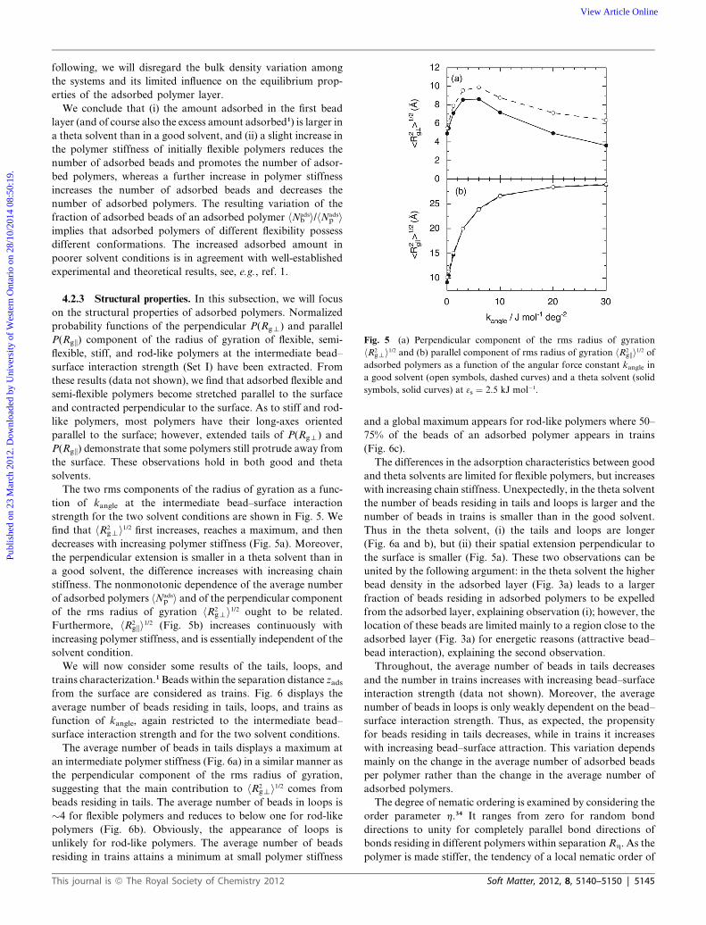
Fig. 5 (a) Perpendicular component of the rms radius of gyration

hR2gti1/2 and (b) parallel component of rms radius of gyration hR2

gki1/2 ofadsorbed polymers as a function of the angular force constant kangle in

a good solvent (open symbols, dashed curves) and a theta solvent (solid

symbols, solid curves) at 3s ¼ 2.5 kJ mol�1.

Publ

ishe

d on

23

Mar

ch 2

012.

Dow

nloa

ded

by U

nive

rsity

of

Wes

tern

Ont

ario

on

28/1

0/20

14 0

8:50

:19.

View Article Online

following, we will disregard the bulk density variation among

the systems and its limited influence on the equilibrium prop-

erties of the adsorbed polymer layer.

We conclude that (i) the amount adsorbed in the first bead

layer (and of course also the excess amount adsorbed1) is larger in

a theta solvent than in a good solvent, and (ii) a slight increase in

the polymer stiffness of initially flexible polymers reduces the

number of adsorbed beads and promotes the number of adsor-

bed polymers, whereas a further increase in polymer stiffness

increases the number of adsorbed beads and decreases the

number of adsorbed polymers. The resulting variation of the

fraction of adsorbed beads of an adsorbed polymer hNadsb i/hNads

p iimplies that adsorbed polymers of different flexibility possess

different conformations. The increased adsorbed amount in

poorer solvent conditions is in agreement with well-established

experimental and theoretical results, see, e.g., ref. 1.

4.2.3 Structural properties. In this subsection, we will focus

on the structural properties of adsorbed polymers. Normalized

probability functions of the perpendicular P(Rgt) and parallel

P(Rgk) component of the radius of gyration of flexible, semi-

flexible, stiff, and rod-like polymers at the intermediate bead–

surface interaction strength (Set I) have been extracted. From

these results (data not shown), we find that adsorbed flexible and

semi-flexible polymers become stretched parallel to the surface

and contracted perpendicular to the surface. As to stiff and rod-

like polymers, most polymers have their long-axes oriented

parallel to the surface; however, extended tails of P(Rgt) and

P(Rgk) demonstrate that some polymers still protrude away from

the surface. These observations hold in both good and theta

solvents.

The two rms components of the radius of gyration as a func-

tion of kangle at the intermediate bead–surface interaction

strength for the two solvent conditions are shown in Fig. 5. We

find that hR2gti1/2 first increases, reaches a maximum, and then

decreases with increasing polymer stiffness (Fig. 5a). Moreover,

the perpendicular extension is smaller in a theta solvent than in

a good solvent, the difference increases with increasing chain

stiffness. The nonmonotonic dependence of the average number

of adsorbed polymers hNadsp i and of the perpendicular component

of the rms radius of gyration hR2gti1/2 ought to be related.

Furthermore, hR2gki1/2 (Fig. 5b) increases continuously with

increasing polymer stiffness, and is essentially independent of the

solvent condition.

We will now consider some results of the tails, loops, and

trains characterization.1Beads within the separation distance zadsfrom the surface are considered as trains. Fig. 6 displays the

average number of beads residing in tails, loops, and trains as

function of kangle, again restricted to the intermediate bead–

surface interaction strength and for the two solvent conditions.

The average number of beads in tails displays a maximum at

an intermediate polymer stiffness (Fig. 6a) in a similar manner as

the perpendicular component of the rms radius of gyration,

suggesting that the main contribution to hR2gti1/2 comes from

beads residing in tails. The average number of beads in loops is

�4 for flexible polymers and reduces to below one for rod-like

polymers (Fig. 6b). Obviously, the appearance of loops is

unlikely for rod-like polymers. The average number of beads

residing in trains attains a minimum at small polymer stiffness

This journal is ª The Royal Society of Chemistry 2012

and a global maximum appears for rod-like polymers where 50–

75% of the beads of an adsorbed polymer appears in trains

(Fig. 6c).

The differences in the adsorption characteristics between good

and theta solvents are limited for flexible polymers, but increases

with increasing chain stiffness. Unexpectedly, in the theta solvent

the number of beads residing in tails and loops is larger and the

number of beads in trains is smaller than in the good solvent.

Thus in the theta solvent, (i) the tails and loops are longer

(Fig. 6a and b), but (ii) their spatial extension perpendicular to

the surface is smaller (Fig. 5a). These two observations can be

united by the following argument: in the theta solvent the higher

bead density in the adsorbed layer (Fig. 3a) leads to a larger

fraction of beads residing in adsorbed polymers to be expelled

from the adsorbed layer, explaining observation (i); however, the

location of these beads are limited mainly to a region close to the

adsorbed layer (Fig. 3a) for energetic reasons (attractive bead–

bead interaction), explaining the second observation.

Throughout, the average number of beads in tails decreases

and the number in trains increases with increasing bead–surface

interaction strength (data not shown). Moreover, the average

number of beads in loops is only weakly dependent on the bead–

surface interaction strength. Thus, as expected, the propensity

for beads residing in tails decreases, while in trains it increases

with increasing bead–surface attraction. This variation depends

mainly on the change in the average number of adsorbed beads

per polymer rather than the change in the average number of

adsorbed polymers.

The degree of nematic ordering is examined by considering the

order parameter h.34 It ranges from zero for random bond

directions to unity for completely parallel bond directions of

bonds residing in different polymers within separationRh. As the

polymer is made stiffer, the tendency of a local nematic order of

Soft Matter, 2012, 8, 5140–5150 | 5145

Fig. 6 Average number of beads residing in (a) tails hNtaili, (b) loopshNloopi, and (c) trains hNtraini of adsorbed polymers as a function of

the angular force constant kangle in a good solvent (open symbols,

dashed curves) and a theta solvent (solid symbols, solid curves) at 3s ¼2.5 kJ mol�1.

Publ

ishe

d on

23

Mar

ch 2

012.

Dow

nloa

ded

by U

nive

rsity

of

Wes

tern

Ont

ario

on

28/1

0/20

14 0

8:50

:19.

View Article Online

bonds in the adsorbed polymer layer increases. Fig. 7 shows the

average bond order hhi for Rh ¼ 20 �A as a function of kangle at

the intermediate bead–surface interactions strength. First, the

bond-order data show virtually no bond order (h z 0.1) for

adsorbed flexible polymers, whereas there is a large bond order

(hz 0.8–0.9) for adsorbed rod-like polymers. The bond order of

adsorbed bonds is basically insensitive to the solvent condition.

Fig. 7 Average bond order hhi as a function of the angular force

constant kangle in a good solvent (open symbols, dashed curves) and

a theta solvent (solid symbols, solid curves) for Rh ¼ 20 �A and at 3s ¼2.5 kJ mol�1.

5146 | Soft Matter, 2012, 8, 5140–5150

Snapshots of the final equilibrium configurations of the MC

simulations for adsorbed flexible and rod-like polymers were

given in Fig. 2 and illustrate a number of properties previously

quantified. For the rod-like polymers, it is obvious that some

polymers strongly protrude into the solution, giving rise to the

tails in P(Rgt) and P(Rgk) discussed above. Similar observations

of ‘‘hairpins’’ extending into solution for adsorbed semi-flexible

polymers in a good solvent have previously been discussed by

Kramarenko et al.14 Furthermore, the change from a disordered

to a nematic-like order of adsorbed polymers at increasing

polymer stiffness was quantified in Fig. 7. Snapshots in the ESI†

(Fig. S5) further illustrate this change of bond order with

increasing stiffness as well as the appearance of a few semi-flex-

ible and rod-like polymers protruding into the solution.

4.3 Dynamic properties

In the BD simulation, polymers diffuse to the surface, become

physically attached, and undergo various structural relaxations.

In the following, t0 will denote the time of the onset of the first

polymer attachments and t0 0 the time at which a quantity has

relaxed to its equilibrium value. As we will see, t0 0 is generally

property dependent. The equilibrium values given below are

taken from the separate MC simulations. Mostly, there is very

good agreement between the equilibrium values obtained from

the MC simulations and the values of the corresponding prop-

erties at the end of the BD simulations.

4.3.1 Adsorbed amount. The adsorption process will first be

characterized by considering the time dependence of the number

of adsorbed beads and of the number of adsorbed polymers.

Fig. 8a shows Nadsb (t) and Fig. 8b shows Nads

p (t) as a function of

the simulation time t in a logarithmic representation for flexible

and rod-like polymers in good and theta solvents at the inter-

mediate bead–surface attraction.

Though the first polymers adsorbed somewhat earlier, Fig. 8

shows that a more substantial rise ofNadsb (t) andNads

p (t) appears at

t0 z 2 ns in the good solvent and t0 z 10 ns in the theta solvent.

There are likely two reasons for this difference: (i) different initial

structures from the MC simulations with a wider region of

reduced polymer density in the theta solvent (see Fig. 2) and

hence a longer distance for the polymers to diffuse and (ii)

a smaller mutual diffusion coefficient in the theta solvent as

compared to that in the good solvent. To discriminate between

these two explanations, shorter and supplementary BD simula-

tions were performed for the two solvent conditions using the

MC structure of the other condition as the initial structures.

These results are also given in Fig. 8 (solid and dashed curves),

and they display that the dominant contribution comes from the

different mutual diffusion coefficient but that the contribution

from the different initial structures is not negligible.

The appearance of a common onset time t0 z 2 ns in the good

solvent and different from t0 z 10 ns in the theta solvent (i) is

consistent with the initial part of the adsorption being diffusion

controlled without any significant drift contribution from the

bead–surface attraction and (ii) the mutual diffusion is at most

marginally affected by the polymer stiffness at the conditions of

this study. As the adsorption process proceeds further, it

becomes faster for rod-like polymers than flexible ones in the

This journal is ª The Royal Society of Chemistry 2012

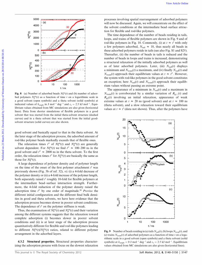
Fig. 8 (a) Number of adsorbed beads Nadsb (t) and (b) number of adsor-

bed polymers Nadsp (t) as a function of time t on a logarithmic scale in

a good solvent (open symbols) and a theta solvent (solid symbols) at

indicated values of kangle in J mol�1 deg�2 and 3s ¼ 2.5 kJ mol�1. Equi-

librium values obtained from MC simulations are also given (horizontal

lines). Data from shorter simulations of flexible polymers in a good

solvent that was started from the initial theta-solvent structure (dashed

curves) and in a theta solvent that was started from the initial good-

solvent structure (solid curves) are also shown.

Fig. 9 Number of beads residing in (a) tailsNtail(t), (b) loopsNloop(t), and

(c) trains Ntrain(t) of adsorbed polymers as a function of time t on a loga-

rithmic scale in a good solvent (open symbols) and a theta solvent (solid

symbols) at kangle ¼ 0 J mol�1 deg�2 and 3s ¼ 2.5 kJ mol�1. Equilibrium

values obtained from MC simulations are also given (horizontal lines).

Publ

ishe

d on

23

Mar

ch 2

012.

Dow

nloa

ded

by U

nive

rsity

of

Wes

tern

Ont

ario

on

28/1

0/20

14 0

8:50

:19.

View Article Online

good solvent and basically equal to that in the theta solvent. At

the later stage of the adsorption process, the adsorbed amount of

rod-like polymer beads markedly exceeds that of flexible ones.

The relaxation times t00 of Nadsb (t) and Nads

p (t) are generally

solvent dependent. For Nadsb (t) we find t00 z 100–200 ns in the

good solvent and t0 0 z 2000 ns in the theta solvent. To the first

order, the relaxation times t00 for Nadsp (t) are basically the same as

those for Nadsb (t).

A large dependence of polymer density and of polymer length

on the time of the onset of the first polymer attachment t0 waspreviously shown (Fig. 3b of ref. 32), viz (i) a 4-fold decrease of

the polymer density or (ii) a 4-fold increase of the polymer length,

both separately raised t0 roughly 10-fold for flexible polymers at

the intermediate bead–surface interaction strength. Further-

more, the 4-fold reduction of the polymer density raised the

adsorption time t0 0 by one order of magnitude.32 Proviso the

different initial configuration and the different final bulk densi-

ties in good and theta solvents, we have here evidence that the

adsorption process becomes slower in poorer solvent conditions.

The dependence of t0 on the polymer stiffness is weak.

Thus, the examination ofNadsb (t) andNads

p (t) and their variation

among the different systems suggests that the relaxation toward

complete adsorption (i) becomes slower in poorer solvent

conditions and (ii) is at later stage of the adsorption process

quantitatively different for flexible and rod-like polymers leading

to different Nadsb (t)/Nads

p (t) ratios, related to different polymer

arrangement in the adsorbed layers.

4.3.2 Structural properties. Structural properties character-

izing the adsorption process with focus on the slowest relaxation

This journal is ª The Royal Society of Chemistry 2012

processes involving spatial rearrangement of adsorbed polymers

will now be discussed. Again, we will concentrate on the effect of

the solvent conditions at the intermediate bead–surface attrac-

tion for flexible and rod-like polymers.

The time dependence of the number of beads residing in tails,

loops, and trains of flexible polymers are shown in Fig. 9 and of

rod-like polymers in Fig. 10. Commonly, (i) at t z t0 with only

a few polymers adsorbed, Ntail z 18, thus nearly all beads in

these adsorbed polymers reside in tails (see also Fig. S1 and S2†).

Thereafter, (ii) the number of beads in tails is reduced and the

number of beads in loops and trains is increased, demonstrating

a structural relaxation of the initially adsorbed polymers as well

as of later adsorbed polymers. Later, (iii) Ntail(t) displays

a minimum and Ntrain(t) a maximum, and (iv) finally Ntail(t) and

Ntrain(t) approach their equilibrium values at t z t0 0. However,

the system with rod-like polymers in the good solvent constitutes

an exception; here Ntail(t) and Ntrain(t) approach their equilib-

rium values without passing an extreme point.

The appearance of a minimum in Ntail(t) and a maximum in

Ntrain(t) is corroborated by a similar variation of Rgt(t) and

Rgk(t) involving an initial relaxation, appearance of weak

extreme values at t z 20 ns (good solvent) and at t z 100 ns

(theta solvent), and a slow relaxation toward their equilibrium

values at t z t0 (data not shown). Thus, after the polymers have

Soft Matter, 2012, 8, 5140–5150 | 5147

Fig. 10 Number of beads residing in (a) tails Ntail(t), (b) loops Nloop(t),

and (c) trains Ntrain(t) of adsorbed polymers as a function of time t on

a logarithmic scale in a good solvent (open symbols) and a theta solvent

(solid symbols) at kangle ¼ 30 J mol�1 deg�2 and 3s ¼ 2.5 kJ mol�1.

Equilibrium values obtained from MC simulations are also given (hori-

zontal lines).

Fig. 11 Probability distribution of the adsorption time P(tads) on a log-

arithmic scale in a good solvent (open symbols) and a theta solvent (solid

symbols) conditions (a) at kangle ¼ 0 (flexible polymers) for early (dotted

curves) and late (solid curves) adsorption and (b) for late adsorption at

kangle¼ 0 (flexible polymers, black) and kangle¼ 30 J mol�1 deg�2 (rod-like

polymers, red); all at 3s ¼ 2.5 kJ mol�1. Adsorption appearing before t ¼t1/2 ¼ 20 ns (good solvent) and 200 ns (poor solvent) were considered as

early, otherwise late.

Publ

ishe

d on

23

Mar

ch 2

012.

Dow

nloa

ded

by U

nive

rsity

of

Wes

tern

Ont

ario

on

28/1

0/20

14 0

8:50

:19.

View Article Online

attained a two-dimensional shape and oriented parallel to the

surface (leading to larger Ntrain), they become laterally

compressed, resulting in fewer anchoring points (leading to

smaller Ntrain) and longer tails (leading to larger Ntail). For

flexible polymers in a good solvent, it was previously shown that

this final lateral compression becomes accentuated at increasing

bead–surface attraction.34 As compared to the good solvent, in

the theta solvent we find here that such a spatial restructuring is

much stronger and also appears for rod-like polymers.

The reason for this larger final spatial restructuring of

adsorbed flexible polymers at poorer solvent conditions (Fig. 9)

is mainly that the adsorbed polymers at intermediate time (t z100 ns) are more strongly attracted to the surface, not through

the direct bead–surface interaction, but indirectly through the

attractive bead–bead interaction. As at this stage the polymers

are individually adsorbed and have only limited contact with

bulk polymers (see Electronic Supplementary Information†),

the polymers coils are two-dimensional and localized parallel to

and at the surface. There is also a secondary effect that the

number of beads in tails at equilibrium is enhanced at poorer

solvent conditions. Here, we anticipated that the thicker

adsorbed layer appearing in the theta solvent (see Fig. 3)

energetically facilitates the tail formation. Turning to rod-like

5148 | Soft Matter, 2012, 8, 5140–5150

polymers (Fig. 10), the final relaxation of Ntail(t) to its equi-

librium values in the theta solvent dominates by the energetic

contribution as the difference between the equilibrium values of

Ntail(t) in good and theta solvents is larger than the differences

of Ntail(t) in good and theta solvents at the intermediate time.

The same holds for Ntrain.

Thus, after the polymers have attained a conformation pref-

erential parallel to the surface, they become laterally compressed,

resulting in fewer anchoring points (smaller Ntrain) and longer

tails (larger Ntail). This compression accentuates at increasing

polymer flexibly and at poorer solvent conditions.

4.3.3 Integration time and residence time. The dynamics of

the adsorption process will now be considered. For that reason,

let the distribution function P(tads) denote the probability that

a polymer remains (continuously) adsorbed during the time tadsafter it has become adsorbed. Obviously, P(0)¼ 1 and P(N)¼ 0.

Furthermore, let t1/2 denote the time at which half of the

maximum adsorbed amount is achieved. In our analysis, we will

separate polymers that adsorbed before t ¼ t1/2 ¼ 20 ns in the

good solvent and t¼ t1/2 ¼ 200 ns in the theta solvent (cf. Fig. 8).

It is anticipated that adsorption properties of polymers adsorb-

ing on a bare surface are different from those of polymers

adsorbing on a surface with adsorbed polymers.

Fig. 11 displays probability distributions of the adsorption

time on a logarithmic scale versus time for different cases.

Generally, lnP(tads) vs tads shows (i) a fast initial decay down to

P(tads) z 10�2 to 10�4 and (ii) thereafter a basically linear

dependence on the adsorption time tads. The time of the onset at

which lnP(tads) starts to become linearly dependent on tads will be

referred to as the integration time sint. Observation (i) implies

This journal is ª The Royal Society of Chemistry 2012

Publ

ishe

d on

23

Mar

ch 2

012.

Dow

nloa

ded

by U

nive

rsity

of

Wes

tern

Ont

ario

on

28/1

0/20

14 0

8:50

:19.

View Article Online

that polymers with an adsorption time tads < sint have a larger

probability (per unit time) of becoming desorbed than those

polymers with an adsorption time tads > sint, whereas observation(ii) implies that for adsorption times tads > sint the desorption

process becomes a first order process and thus all adsorbed

polymers with tads > sint display the same probability of being

desorbed. Polymers with an adsorption time tads < sint are

considered as not yet being fully integrated in the adsorbed layer,

whereas those with tads > sint are considered as fully integrated.

The slope sres of lnP(tads) vs tads, tads > sint, provides the residencetime (average adsorption time) of fully integrated polymers. The

extracted integration sint and residence sres times are compiled in

Table 3.

In more detail, Fig. 11a shows P(tads) for adsorbed flexible

polymers in the good (open symbols) and the theta (solid

symbols) solvent separated for polymers being adsorbed early

(t < t1/2) and late (t > t1/2). The quasi-linear regimes after ca. 25 ns

falls off with different slopes, and obviously the residence time of

adsorbed polymers is longer for those being adsorbed at an early

stage (dotted curves). The difference is significant in the good

solvent and large in the theta solvent. Hence, polymers adsorbing

on a bare surface have a longer residence times than polymers

adsorbing on a polymer covered surface.

Fig. 11b displays also P(tads) but now for flexible and rod-

like polymers at the two solvent conditions. We find that the

integration times, sint ¼ 15–30 ns, do not strongly depend on

the polymer flexibility or the solvent conditions but are in

most cases significantly shorter than the residence times sres ¼30–100 ns. The residence times are longer for the rod-like

polymers as compared to the flexible ones—an observation

that could be understood by their larger contact and hence

adsorption energy with the surface. Furthermore, the residence

times in the theta solvent is smaller than those in the good

solvent. Here, the larger number density of beads outside the

layer comprising the primary adsorbed beads most likely

facilitate the exchange of polymers. Thus, the presence of

polymers available for an exchange appears more important

than any obstruction effect.

Hence, we have defined the time for a polymer to become fully

integrated into the adsorbed layer. Moreover, it was found that

the residence time of fully integrated polymers (i) is smaller for

flexible polymers as compared to rod-like ones and (ii) is smaller

in a theta solvent as compared to a good solvent.

Table 3 Integration time and residence time of integrated polymersa

Solvent kangle/J mol�1 deg�2 sint/ns sres/ns

Good 0 20 45Good 30 30 100Theta 0 15 30Theta 30 25 65

a The integration time sint is taken as the adsorption time at the onsetwhere the adsorption probability distribution P(tads) displays an

exponential behavior according to PðtadsÞ ¼ Ce�ðtads=sresÞ. The timeconstant sres of the exponential behavior is taken as the residence timeof fully integrated polymers. Estimated uncertainties are 50% (sint) and10% (sres).

This journal is ª The Royal Society of Chemistry 2012

5 Summary

The adsorption of uncharged 20-mers onto planar surfaces from

good and theta solvents has been studied for different intrinsic

stiffnesses of the polymers and various bead–surface attractions.

Equilibrium adsorption properties of 12 systems were deter-

mined by Monte Carlo simulations, and adsorption processes of

these were determined by Brownian dynamic simulations.

The layer of adsorbed polymers at the surface increased when

changing from good to theta solvents. At theta conditions, the

distribution of polymer beads becomes oscillatory, and the

individual polymers in the first adsorption layers became less

anchored to the surface.

The adsorption process started from a polymer-free surface

and the initial adsorption was diffusion controlled, but soon

became governed by the bead–surface attraction. The adsorption

was slower in the theta solvent mainly due to a slower mutual

diffusion. Flexible polymers became flattened after attaching,

but the final relaxation mechanism involved an increased

perpendicular extension with fewer adsorbed beads and longer

tails driven by the surface pressure originating from the

surrounding adsorbed polymers. This structural rearrangement

becomes stronger in poorer solvent conditions. The residence

times of adsorbed polymers became longer with increasing

polymer stiffness and smaller in poorer solvent conditions, the

latter effect consistent with a weakening of the anchoring of

adsorbed polymers.

Acknowledgements

Generous allocation of computer resources by Center for

Scientific and Technical Computing at Lund University

(LUNARC) and financial support by the Swedish Research

Council (VR), grant number 621-2007-5251, are gratefully

acknowledged.

References

1 G. J. Fleer and J. Lyklema, in Adsorption From Solution at the Solid/Liquid interface, Academic Press, New York, 1983.

2 D. F. Evans and H. Wennerstr€om, The Colloidal Domain: WherePhysics, Chemistry, Biology and Technology Meet, Wiley-VCH, NewYork, 2nd edn, 1999.

3 W. Norde, Colloids and Interfaces in Life Sciences, Marcell DekkerInc., New York, 2003.

4 J. J. Gray, Curr. Opin. Struct. Biol., 2004, 14, 110.5 M. Yaseen, H. J. Salacinski, A. M. Seifalian and J. R. Lu, Biomed.Mater., 2008, 3, 034123.

6 T. Ramanathan, A. A. Abdala, S. Stankovich, D. A. Dikin,M. Herrera-Alonso, R. D. Piner, D. H. Adamson, H. C. Schniepp,X. Chen and R. S. Ruoff, et al., Nat. Nanotechnol., 2008, 3, 327.

7 G. J. Fleer, M. A. Cohen Stuart, J. H. M. H. Scheutjens, T. Cosgroveand B. Vincent, Polymers at interfaces, Chapman & Hall, London,1993.

8 M. A. Cohen Stuart and G. J. Fleer, Annu. Rev. Mater. Sci., 1996, 26,463.

9 A. Yethiraj, Adv. Chem. Phys., 2002, 121, 89.10 M. A. Cohen Stuart, Surf. Sci. Ser., 2003, 110, 1.11 B. O’Shaughnessy and D. Vavylonis, J. Phys.: Condens. Matter, 2005,

17, R63.12 J. M. H. M. Scheutjens and G. J. Fleer, J. Phys. Chem., 1980, 84, 178.13 P. G. de Gennes, Macromolecules, 1981, 14, 1637.14 E. Yu. Kramarenko, R. G. Winkler, P. G. Khalatur, A. R. Khokhlov

and P. Reineker, J. Chem. Phys., 1996, 104, 4806.15 A. Striolo and J. M. Prausnitz, J. Chem. Phys., 2001, 114, 8565.

Soft Matter, 2012, 8, 5140–5150 | 5149

Publ

ishe

d on

23

Mar

ch 2

012.

Dow

nloa

ded

by U

nive

rsity

of

Wes

tern

Ont

ario

on

28/1

0/20

14 0

8:50

:19.

View Article Online

16 T. Sintes, K. Sumithra and E. Straube, Macromolecules, 2001, 34,1352.

17 A. Striolo, A. Jayaraman, J. Genzer and C. K. Hall, J. Chem. Phys.,2005, 123, 064710.

18 R. Hasegawa and M. Doi, Macromolecules, 1997, 30, 3086.19 L.-C. R. Jia and P. Y. Lai, J. Chem. Phys., 1996, 105, 11319.20 R. Zajec and A. Chakrabarti, J. Chem. Phys., 1996, 104, 2418.21 H. Takeuchi, Macromol. Theory Simul., 1999, 8, 391.22 A. L. Ponomarev, T. D. Sewell and C. J. Durning, Macromolecules,

2000, 33, 2662.23 J. K. Wolterink, G. T. Barkema and M. A. Cohen Stuart,

Macromolecules, 2005, 38, 2009.24 G. D. Smith, Y. Zhang, F. Yin and D. Bedrov, Langmuir, 2006, 22,

664.25 R. Descas, J.-U. Sommer and A. Blumen, J. Chem. Phys., 2006, 124,

094701.26 K. A. Smith, M. Vladkov and J.-L. Barrat,Macromolecules, 2005, 38,

571.27 V. A. Harmandaris, K. Ch Daoulas and V. G. Mavrantzas,

Macromolecules, 2005, 38, 5796.28 K. Ch Daoulas, V. A. Harmandaris and V. G. Mavrantzas,

Macromolecules, 2005, 38, 5780.

5150 | Soft Matter, 2012, 8, 5140–5150

29 Y. Li, D. Wei, C. C. Han and Q. Liao, J. Chem. Phys., 2007, 126,204907.

30 A. Chremos, E. Glynos, V. Koutsos and P. J. Camp, Soft Matter,2009, 5, 637.

31 N. K€allrot and P. Linse, Macromolecules, 2007, 40, 4669.32 N. K€allrot, M. Dahlqvist and P. Linse, Macromolecules, 2009, 42,

3641.33 N. K€allrot and P. Linse, J. Phys. Chem. B, 2010, 114, 3741.34 N. K€allrot and P. Linse, Macromolecules, 2010, 43, 2055.35 J. Baschnagel, H. Mayer, F. Varnik, S. Metzger, M. Aichele,

M. M€uller and K. Binder, Interface Sci., 2003, 11, 159.36 J. P. de Gennes, Scaling Concepts in Polymer Physics, Cornell

University Press, Ithaca, 1979.37 M. Ullner, B. J€onsson, C. Peterson, O. Sommelius and B. S€oderberg,

J. Chem. Phys., 1997, 107, 1279.38 A. Akinchina and P. Linse, Macromolecules, 2002, 35, 5183.39 MOLSIM, Version 4.7, P. Linse, Lund University, Sweden,

2009.40 M. P. Allen and D. J. Tildesley, Computer Simulations of Liquids,

Oxford University Press, Oxford, 1987.41 D. L. Ermak and J. A. McCammon, J. Chem. Phys., 1978, 69(4),

1352.

This journal is ª The Royal Society of Chemistry 2012