effect of pulse-shape uncertainty on the accuracy of deconvolved lidar profiles

Dreischuh et al. Vol. 12, No. 2 /February 1995 /J. Opt. Soc. Am. A 301

Effect of pulse-shape uncertainty on theaccuracy of deconvolved lidar profiles

T. N. Dreischuh, L. L. Gurdev, and D. V. Stoyanov

Institute of Electronics, Bulgarian Academy of Sciences, 72 Tzarigradsko Shosse Boulevard, 1784 Sofia, Bulgaria

Received February 7, 1994; revised manuscript received August 8, 1994; accepted August 9, 1994

The effect of random and deterministic pulse-shape uncertainties on the accuracy of the Fourier deconvolutionalgorithm for improving the resolution of long-pulse lidars is investigated theoretically and by computersimulations. Various cases of pulse uncertainties are considered including those that are typical of Dopplerlidars. It is shown that the retrieval error is a consequence of two main effects. The first effect consistsof a shift up or down (depending on the sign of the uncertainty integral area) of the lidar profile as a whole,proportionally to the ratio of the pulse uncertainty area to the true pulse area. The second effect consistsof additional amplitude and phase distortions of the spectrum of the small-scale inhomogeneities of the lidarprofile. The results obtained allow us to predict the order and the character of the possible distortions andto choose ways to reduce or prevent them.

1. INTRODUCTIONThe lidar systems that use long sensing laser pulses (e.g.,emitted by a TE (TEA) CO2 laser1,2 have low spatialresolution that is of the order of the pulse length if theintegration period of the photodetector is negligible. Inthis case the lidar return signal F std at moment t afterthe pulse emission is described by the convolution3

F std Z `

2`

Sst 2 2z0ycdFsz0ddz0 (1)

of the pulse shape Ssq d and the maximum-resolved (ob-tainable by a sufficiently short laser pulse) lidar profileFszd. In Eq. (1), c is the speed of light, z0 is the coor-dinate along the line of sight, Ssq d P sq dyPp, P sq d isthe pulse power shape and Pp is its peak value, and q isa time variable. As a result of the convolution effect inthe case of CO2 Doppler lidars that is mentioned in Refs. 4and 5, important information about the small-scale varia-tions of the backscattering within the long-resolution cell(typically 200–500 m) is lost during the Doppler velocitymeasurements. This loss of information expresses thewell-known conflict between the range and the velocityresolutions in Doppler radars and lidars. An approachfor retrieval of the mean atmospheric backscattering co-efficient and its fluctuations has been developed in Refs. 6and 7 for CO2 differential absorption lidar measurements.This approach is based on the so-called correction functionand requires some preliminary information (provided bythe differential absorption lidar technique) about the at-mospheric absorption and about the relation between theabsorption and the scattering.

A direct way to improve the lidar resolution is tosolve Eq. (1) with respect to Fszd. That is why ear-lier we developed8,9 deconvolution techniques to invertEq. (1) when the pulse shape is known without any un-certainty. These techniques are based on Fourier trans-formation, the Volterra integral equation, or a recurrencerelation and ensure good quality in the retrieval of the finestructure of the backscattering inhomogeneities. Such

0740-3232/95/020301-06$06.00

an approach is essential for single-wavelength Doppler li-dars. It does not require preliminary information aboutthe absorption or about the spatial spectra of the in-homogeneities. As a result, the range resolution of thebackscattering profiles becomes better than that of the ve-locity profiles. The application of the deconvolution tech-niques to Doppler lidar data from the National Oceanicand Atmospheric Administration was demonstrated inRefs. 10 and 11, in which some of the statistical char-acteristics of the data within the Doppler resolution cellhad been determined.

As briefly noted in Refs. 8 and 12, because of variousfactors the shape Ssq d might be determined with someregular (deterministic) or random uncertainties that leadto errors in the determination of Fszd. As an example,the spike in the laser pulse shape of TEA CO2 Dopplerlidars is often not well recorded; i.e., it is cut, in the outputraw data.13 The purpose of the present study, being ina sense an addition to that of Ref. 8, is to investigate therelations between the pulse-shape uncertainties and thecorresponding errors in the restoration of the lidar profilesFszd. This problem is of importance for the analysis ofthe limitations of the deconvolution techniques as well asfor the analysis of the requirements that are satisfied bythe lidar data recorders.

2. PULSE-UNCERTAINTY INFLUENCEON THE ACCURACY OF THEDECONVOLVED LIDAR PROFILESThe Fourier deconvolution algorithm is based on theexpression8

Fsz ; cty2d spcd21Z `

2`

fF̃ svdyS̃svdgexps2jvtddv , (2)

where S̃svd R`

2` Sst0 dexps jvt0 ddt0 and F̃ svd R`

2` F st0 dexps jvt0 ddt0 are Fourier transforms of S and F,respectively; j is imaginary unity; and F̃svd ; F̃s2vycd F̃ svdyS̃svd scy2d

R`

2` Fsz0 ct0y2dexps jvt0 ddt0. Let

1995 Optical Society of America

302 J. Opt. Soc. Am. A/Vol. 12, No. 2 /February 1995 Dreischuh et al.

us represent the measured pulse shape Smsq d as asum Smsq d Ssq d 1 f sq d of the true pulse shape Ssq dand a deterministic or random uncertainty f sq d in itsmeasurement. Then the Fourier deconvolution error isobtained on the basis of Eq. (2) as

dFsz cty2d Frszd 2 Fszd

2 spcd21Z `

2`

F̃svdf̃ svdfS̃svd 1 f̃ svdg21

3 exps2jvtddv , (3)

where Frszd is the lidar profile restored with use ofthe measured pulse shape Smsq d and f̃ svd

R`

2` f sq dexps jvq ddq is the Fourier transform of f sq d. As far asF̃svd, S̃svd, and f̃ svd are expressible as integrals over allvalues of a spatial variable z0 ct0y2, Eq. (3) does notrepresent, in general, a local dependence of dFszd on Fszdand f szd.

The Fourier transformation of Eq. (3) leads to the re-lation d̃FsvdS̃msvd 2s2ycdF̃svdf̃ svd, where S̃msvd S̃svd 1 f̃ svd, and d̃Fsvd

R`

2` dFsz cty2dexps jvtddtare the Fourier transforms of Smsq d and dFsz cty2d,respectively. The inverse Fourier transform of the lastrelation leads to the equation

Sm p dF 2f p F , (4)

which expresses the nonlocal interconnection between theuncertainty f and the error dF (p denotes a convolution).The sense of Eq. (4) is that, for instance, a positive-signuncertainty f sq d . 0 is equivalent to a pseudocontributionto the integration in Eq. (1) [to the signal F std]. Corre-spondingly, the deconvolution process compensates thispseudocontribution by lowering the restored profile Fr

with respect to F.

A. Deterministic UncertaintiesHere we analyze some general features of the influenceof different types of deterministic uncertainty on the re-trieval accuracy. Let us first consider f sq d as a slowlyvarying [in comparison with Ssq d] prolonged determin-istic function of q with constant sign and assume thatf sq d ,, Ssq d. Correspondingly, the spectrum f̃ svd willbe narrow compared with S̃svd and will be concentratedaround v 0. Then we may neglect f̃ svd in the inte-grand denominator of Eq. (3) and integrate over v, consid-ering S̃svd to be a constant equal to S̃s0d

R`

2` Ssq ddq teff , which may be interpreted as the effective pulse du-ration. In this way, from Eq. (3) we obtain the followingexpression for dF:

dFsz cty2d ø 2peff21

Z `

2`

Fsz0 df st 2 2z0ycddz0

2s punypeff dFstd . (5)

Relation (5) shows that the error dF is proportional tothe magnitudes of F and f and involves interactionsof f with all values of F within the spatial interval ofthe uncertainty. In relation (5), peff scy2dteff, pun scy2d

R`

0 f sq ddq , and the value of F pun21s f p Fd may

be interpreted as being weighted by the uncertainty av-erage of F. Here peff and pun may be considered to besome effective pulse and uncertainty areas, respectively.

In general, the uncertainty area pun is an integral char-acteristic of the uncertainty effect. It may be positive ornegative or even equal to zero for uncertainties with al-ternating signs.

A typical case of a fast-varying short-range uncertaintyis the cut of a pulse spike. This case is essential forthe CO2 Doppler lidars. Here we may consider the pulseshape as a sum Ssq d fS sq d 1 fR sq d of the spike fS sq dand the remaining tail fR sq d. Thus Smsq d fR sq d andf sq d 2fS sq d so that Eq. (4) acquires the form fS p F fR p dF from which, taking into account that fS p F øpS F, one may write

dFstdyFstd ø pSypR . (6)

In relation (6), pS scy2dR`

0 fS sq ddq is the effectivespike area, pR scy2d

R`

0 fR sq ddq is the effective remain-der area, and dFstd pR

21s fR p dFd may be interpreted asa weighted, by the remainder, average of dF. It can beseen that the weighted error dF . 0 and that the relativeweighted error dFyF is a positive constant approximatelyequal to pSypR . This positive tendency suggests that aspike cut causes an elevation proportional to pSypR ofFr as a whole with respect to F. Such an effect can beexpected because the spike cut is a negative-sign uncer-tainty f sq d 2fS sq d.

For a more detailed analysis of the spike-cut influenceon the retrieval accuracy, we may consider the profile Fstdto be a sum Fstd Fsmstd 1 Fvstd of a smooth componentFsmstd and a fast-varying component Fvstd describing thesmall-scale inhomogeneities of Fstd. The mechanism ofthe uncertainty effect on the retrieval accuracy can beunderstood by analysis of the error in the restoration ofthe smooth component Fsmstd and in one of the harmonic(sine, cosine) components F0std of the spectrum of thesmall-scale inhomogeneities. Then Eq. (3) acquires theform

dFsz cty2d 2spcd21sJ1 1 J2d , (7a)

where

J1 Z `

2`

F̃smsvdF svdexps2jvtddv , (7b)

J2 Z `

2`

F̃0svdF svdexps2jvtddv , (7c)

and F svd f̃ svdfS̃svd 1 f̃ svdg21. F̃smsvd R

`

2` Fsmstdexps jvtddt and F̃0svd

R`

2` F0stdexps jvtddt are theFourier transforms of Fsmstd and F0std, respectively.For a spike cut we have f̃ svd 2f̃S svd 2

R`

2` fS sq dexps jvq ddq and S̃svd 1 f̃ svd f̃R svd

R`

2` fR sq dexps jvq ddq . Since a spike is short compared withFsmstd and F0std, its spectral width Dv exceeds thespectral widths Dvsm and Dv0 of F̃smsvd and F̃0svd.The spectral width DvR of f̃R svd satisfies the inequalityDv .. DvR .. sDvsm, Dv0d because the pulse remainderfR std is shorter than Fstd and F0std but is longer thanfS std. If the spike is shorter than the oscillation periodT0 2pyv0 of F0std so that Dv . v0, the integrationin J1 is restricted by the profile of F̃smsvd and is con-centrated around v 0, where f̃ svd 2f̃S svd ø 2f̃S s0d


and S̃svd 1 f̃ svd f̃Rsvd ø f̃R s0d. Similarly, the in-tegration in J2 is concentrated around the peak fre-quencies v 6v0 of F̃0svd, where f̃ svd ø 2f̃S s0d andS̃svd 1 f̃ svd ø f̃R s6v0d. Then by using Eqs. (7b) and(7c) we obtain that

J1 2pcs pSypR dFsmsz cty2d , (8a)

J2 2pcf pSypR sv0dg hcosfwR sv0dgF0sz cty2d

1 2 sinfwRsv0dgspcd21 ImfJasz cty2dgj , (8b)

where pR svd scy2djf̃R svdj and wR svd argf f̃R svdg.The symbols j ? j and argf?g denote the module and the ar-gument, respectively, of a complex quantity. The quan-tity Jastd

R `

0 F0svdexps2jvtddv is the analytical signalof spcdF0std, and its imaginary part ImfJag is connected toits real part RefJag spcy2dF0std by the Hilbert transfor-mation. That is, ImfJastdg p21P

R`

2` hRefJast0 dgyst 2

t0 dj dt0 scy2dPR`

2` fF0st0 dyst 2 t0 dgdt0, where P de-notes the principal value of the integral at the sin-gular point t0 t. Thus for a sine function F0std A0 sinsv0td (A0 is the dimensional amplitude) we ob-tain that ImfJastdg 2spcy2dA0 cossv0td. For a co-sine function F0std A0 cossv0td we obtain ImfJastdg spcy2dA0 sinsv0td. In both cases, on the basis ofEqs. (7a), (8a), and (8b) we obtain the following estimateof the error caused by a spike cut:

dFsz cty2d ø s pSypRdFsmsz cty2d

1 f pSypRsv0dgF0fz 2 zshsv0dg , (9)

where zshsvd cwR svdys2vd is a spatial phase shift ofthe error oscillations with respect to the oscillations ofF0. The first term on the right-hand side of relation (9)describes an elevation of the smooth component Fsmszdproportional to pSypR that leads to an elevation of Fr

as a whole with respect to F. The second term describesboth an increase in the amplitude of the oscillatory compo-nent F0sz cty2d proportional to pSypR sv0d and a phaseshift zshsv0d of its oscillations. It can be seen that thesetwo effects are frequency dependent. It means that thespike cut leads to distortion of the spectrum of the in-homogeneities of the restored lidar profile in comparisonwith the spectrum of the original profile. The frequencydependence of the second term on the right-hand side ofrelation (9) is determined only by the spectrum f̃R svd ofthe remainder pulse. This is a consequence of the as-sumption that the spike cut is shorter than the period T0.Then the influence of the spike spectrum is negligible be-cause f̃S svd ø f̃Ss0d.

To complete the analysis of deterministic uncertain-ties, we briefly consider the case of uncertainties with al-ternating signs having oscillatory character, e.g., f std Imfastdexps jvf tdg, where astd . 0 is the amplitude func-tion. We assume that the uncertainty duration is of theorder of the pulse duration, so the spectrum f̃ svd willhave a peak at v vf and will be wider than F̃smsvdand F̃0svd. Under these conditions we may considerf̃ svd, S̃svd, and consequently F̃ svd to be slowly varyingfunctions of v within the essential integration intervalsaround v 0 and v 6v0. Then, following the sameprocedure as in the case of a pulse cut, on the basis of

Eqs. (7a)–(7c) we obtain an estimate of the retrieval er-ror in the form

dFsz cty2d ø 2s punypeff dFsmsz cty2d

2 jF sv0djF0fz 2 zshsv0dg , (10)

where zshsvd scy2vdargfF svdg is a spatial phase shift.Relation (10) shows that the uncertainty leads, propor-tionally to punypeff , to an elevation or a lowering (depend-ing on the sign of pun) of Fr as a whole with respectto F. Besides, the second term on the right-hand sideof relation (10) indicates additional amplitude and phasedistortions of F0 (see as well the case of the pulse cut).

B. Random UncertaintiesIn this subsection we consider the retrieval errors causedby random uncertainties with correlation time tc .. teff ,by fluctuating spike cuts, and by random uncertaintieswith correlation time tc ,, teff .

In the first case, when tc .. teff , the whole measuredpulse shape fluctuates from shot to shot. Then by use ofEq. (4) we estimate the corresponding rms error as

sFsz cty2d kjdFsz cty2dj2l1/2 ø sspunypeff dFstd ,

(11)

where kpunl 0 and kpun2l1/2 spun ; k?l denotes ensem-

ble average. According to relation (11), an averaging ofSmsq d over a number N of laser shots, before applicationof Eq. (2), will reduce sF

pN times because of the reduc-

tion of spun in the same proportion.A fluctuating spike cut may arise even at a stable pulse

shape with a short spike because of the fluctuations of thepositions of the sampling pulses with respect to the laserpulse emission. In this case we may neglect the fluctua-tions of pR and pR sv0d and use relation (9) to determinethe statistical retrieval error s ssm

2 1 sr2d1/2, where

s2 kdF2l, sm kdFl, and sr ksdF 2 smd2l1/2. Obvi-

ously, the expression of s has the same form as that ofrelation (9), where pS should be replaced by k pS

2l1/2 sk pSl2 1 DpSd1/2; DpS ks ps 2 k pS ldl2.

Let us further consider f sq d as a random function withzero mean value, variance Df sq d sf

2sq d kjf sq d2jl (sf

is the standard deviation), and correlation time tc ,, teff .A possible (statistically) quasi-stationary model of f sq d is

f sq d sf sq df̃ sq d , (12)

where f̃ sq d is a statistically stationary Gaussian-distributed and Gaussian-correlated zero-mean randomfunction with variance Df̃ 1 and correlation time tc.The value of sf sq d does not change essentially withintime intervals of the order of tc. The variance Df maybe modeled as Df sq d g2S2sqd, where 0 , g # 1. At agiven realization of f sq d the retrieval error dF is describedby Eq. (3) or Eqs. (7a)–(7c). It is reasonable to assumethat when f sq d is many times as long as tc, its spectralamplitude profile jf̃ svdj will closely follow the profile ofkjf̃ svdj2l1/2 / fIf svdg1/2, where If svd is the power spectrumof f sq d. Consequently, the spectral width Dv of f̃ is ofthe order of that of If svd, i.e., Dv , tc

21. When tc ,, T0,the spectral width Dv .. v0 and we may assume that inEqs. (7b) and (7c), f̃ svd ø f̃ sv0d ø f̃ s0d. If, in addition,


q ,, 1, we have f̃ s0d ,, S̃s0d. Then in the well-knownprocedure of using Eqs. (7b) and (7c) we obtain that

dFsz cty2d ø 2spunypeff d hFsmsz cty2d

1 jFrsv0djF0fz 2 zshsv0dgj , (13a)

whereFrsvd peffyf peff svd 1 pung,peff svd scy2dR

`

0 Sst0 dexps jvt0 ddt0, and zshsvd scy2vdargfFrsvdg. One cansimplify the factor Frsv0d by neglecting pun in its denom-inator when jpunj ,, jpeff sv0dj. If pun . jpeffsv0dj, onecan preliminarily average Smsq d over N laser shots toa certain extent when jpunj ,, jpeff sv0dj, where pun isthe area of the average uncertainty f sq d. Then Frsv0d øpeffypeff sv0d, and the rms error s kjdFj2l1/2 is describedby relation (13a), in which one should replace 2pun withthe quantity spuny

pN . For a quasi-stationary random

process f sq d [Eq. (12)] the value of spun scy2dstqtcd1/2,where tc

R`

2` Kstddt is the correlation time of f sq d,Kstd k f̃ sq df̃ sq 1 tdl is the correlation coefficient of f̃ sq d,and tq

R `

2` sf2sq ddq . Thus we obtain that

s fstqtcd1/2ysN1/2teff dg hFsmsz cty2d

1 jFr sv0djF0fz 2 zshsv0dgj , (13b)

i.e., s / stcyNd1/2. Certainly, the general principle re-mains valid. That is, the retrieval error is proportionalto the ratio of the uncertainty area (in a statistical sense)to the true pulse area, with additional amplitude andphase distortions of the spectrum of the inhomogeneitiesof Fstd.

3. SIMULATIONSIn the simulations conducted below, we use a model ofFszd described earlier in Ref. 8. This model (Fig. 1) con-sists of a smooth component Ast 2 t0d23 expf2Gst 2 t0dg,a high-resolution component C sin2f2pst 2 t0dyT g for t0 #

t # G 1 t0 at near distances, and a double-peak structureintroducing discontinuities at a relatively far range, whichis given by the expressions D 1 d2 2 st 2 ta 2 dTpd2yTp

2

for ta # t # ta 1 2dTp, and D 1 d2 2 st 2 ta 2 3dTpd2yTp2

for ta 1 2dTp # t # ta 1 4dTp. The parameters arespecified as follows: A 3000 ms3, G 20 ms, C 0.1, T 5 ms, d 0.25, D 0.03, t0 4 ms, ta 70 ms,and Tp 7 ms. In Fig. 1 and in the following figures theabscissa is given in samples where a sample is assumedto be equal to 15 m corresponding to 0.1 ms. The modelof the pulse shape Ssq d (typical for CO2 Doppler lidars)is described by the expression

Ssq d q fsp

2eyt1dexps2q 2yt12d

1 s xeyt2dexps2qyt2dgySp , (14)

where Sp is the peak value of the numerator. The con-stants t1, t2, and x may have various values in order toproduce various shapes. A pulse shape with parameterst1 0.1 ms, t2 2 ms, and x 0.2 is shown in Fig. 1.

First, we modeled a smooth uncertainty as a parabolaf sq d Af1 2 s2q 2 t0d2yt0

2g (for 0 # q # t0), which

is added to or subtracted from the true shape Ssq d; A

and t0 are the parameters to be adjusted. The simu-lations conducted show that the retrieval error is ap-proximately equal to 2spunypeff dFstd [see relation (5)].An illustration of the influence of a parabolic uncer-tainty with parameters A 0.025 and t0 12 msis given in Fig. 2(a). The pulse shape used is givenin Fig. 1. The obtained error dFszd is compared inFig. 2(b) with the approximate dependence [relation (5)],which turns out to describe the behavior of dF cor-rectly. One can see that Frszd is lowered with respect

Fig. 1. Models of the original short-pulse lidar profile and (in-set) of a laser pulse shape (with t1 0.1 ms, t2 2 ms, andx 0.2) as a functions of sample number.

Fig. 2. (a) Original profile (dashed curve) and the profile re-stored by use of Fourier deconvolution (solid curve) in the caseof parabolic uncertainty with A 0.025 and t0 12 ms; (b)obtained (solid curve) and estimated [Eq. (4), dashed curve]errors corresponding to the data of Fig. 2(a).


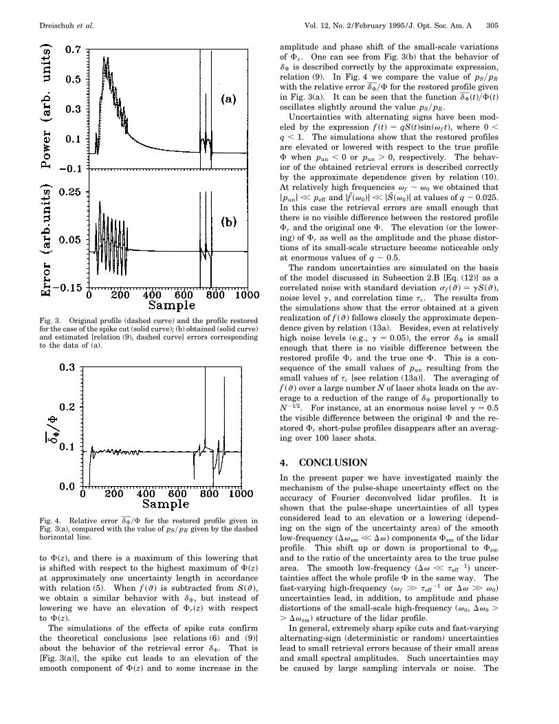
Fig. 3. Original profile (dashed curve) and the profile restoredfor the case of the spike cut (solid curve); (b) obtained (solid curve)and estimated [relation (9), dashed curve] errors correspondingto the data of (a).

Fig. 4. Relative error dFyF for the restored profile given inFig. 3(a), compared with the value of pSypR given by the dashedhorizontal line.

to Fszd, and there is a maximum of this lowering thatis shifted with respect to the highest maximum of Fszdat approximately one uncertainty length in accordancewith relation (5). When f sq d is subtracted from Ssq d,we obtain a similar behavior with dF, but instead oflowering we have an elevation of Frszd with respectto Fszd.

The simulations of the effects of spike cuts confirmthe theoretical conclusions [see relations (6) and (9)]about the behavior of the retrieval error dF. That is[Fig. 3(a)], the spike cut leads to an elevation of thesmooth component of Fszd and to some increase in the

amplitude and phase shift of the small-scale variationsof Fz. One can see from Fig. 3(b) that the behavior ofdF is described correctly by the approximate expression,relation (9). In Fig. 4 we compare the value of pSypR

with the relative error dFyF for the restored profile givenin Fig. 3(a). It can be seen that the function dFstdyFstdoscillates slightly around the value pSypR .

Uncertainties with alternating signs have been mod-eled by the expression f std qSstdsinsvf td, where 0 ,

q , 1. The simulations show that the restored profilesare elevated or lowered with respect to the true profileF when pun , 0 or pun . 0, respectively. The behav-ior of the obtained retrieval errors is described correctlyby the approximate dependence given by relation (10).At relatively high frequencies vf , v0 we obtained thatjpunj ,, peff and jf̃ sv0dj ,, jS̃sv0dj at values of q , 0.025.In this case the retrieval errors are small enough thatthere is no visible difference between the restored profileFr and the original one F. The elevation (or the lower-ing) of Fr as well as the amplitude and the phase distor-tions of its small-scale structure become noticeable onlyat enormous values of q , 0.5.

The random uncertainties are simulated on the basisof the model discussed in Subsection 2.B [Eq. (12)] as acorrelated noise with standard deviation sf sq d gSsq d,noise level g, and correlation time tc. The results fromthe simulations show that the error obtained at a givenrealization of f sq d follows closely the approximate depen-dence given by relation (13a). Besides, even at relativelyhigh noise levels (e.g., g 0.05), the error dF is smallenough that there is no visible difference between therestored profile Fr and the true one F. This is a con-sequence of the small values of pun resulting from thesmall values of tc [see relation (13a)]. The averaging off sq d over a large number N of laser shots leads on the av-erage to a reduction of the range of dF proportionally toN21/2. For instance, at an enormous noise level g 0.5the visible difference between the original F and the re-stored Fr short-pulse profiles disappears after an averag-ing over 100 laser shots.

4. CONCLUSIONIn the present paper we have investigated mainly themechanism of the pulse-shape uncertainty effect on theaccuracy of Fourier deconvolved lidar profiles. It isshown that the pulse-shape uncertainties of all typesconsidered lead to an elevation or a lowering (depend-ing on the sign of the uncertainty area) of the smoothlow-frequency sDvsm ,, Dvd components Fsm of the lidarprofile. This shift up or down is proportional to Fsm

and to the ratio of the uncertainty area to the true pulsearea. The smooth low-frequency sDv ,, teff

21d uncer-tainties affect the whole profile F in the same way. Thefast-varying high-frequency svf .. teff

21 or Dv .. v0duncertainties lead, in addition, to amplitude and phasedistortions of the small-scale high-frequency (v0, Dv0 .

. Dvsm) structure of the lidar profile.In general, extremely sharp spike cuts and fast-varying

alternating-sign (deterministic or random) uncertaintieslead to small retrieval errors because of their small areasand small spectral amplitudes. Such uncertainties maybe caused by large sampling intervals or noise. The


slowly varying prolonged uncertainties may lead to no-ticeable errors, but they may be avoided by suitable choiceof the sampling interval. A known way to reduce therandom uncertainty influence (except for spike cuts) is toaverage the pulse shape over a large number N of laserpulses. The simple expression derived here for this caseand supported by computer simulations allows us to esti-mate the error and to predict the value of N that is nec-essary for achieving a prescribed accuracy.

The exact expression and the approximate estimates ofthe retrieval error dF obtained in this paper allow us, ata known order and character of the error of the pulse-shape recorder, to estimate what type of details of thelidar profile can be restored satisfactorily. In this casethe error magnitude jdFj should be much less than theamplitudes of the lidar profile components of interest, soone can determine the limitations of the Fourier deconvo-lution technique. On the other hand, beginning from therequirements for the quality of the lidar profile restora-tion, one can formulate the requirements for the accuracyof the pulse-shape recorders.

ACKNOWLEDGMENTSThe authors are grateful to one of the anonymous re-viewers of Ref. 8 for directing their attention to the im-portance of the problem investigated in this paper. Theresearch described in this paper was supported in part byBulgarian National Science Foundation grant F-63.

The authors may be contacted by e-mail, ie@bgcict, orfax, 011 (359-2) 757 053.

REFERENCES1. J. Gilbert, J. L. Lachambre, F. Rheault, and R. Fortin, “Dy-

namics of the CO2 atmospheric pressure laser with trans-verse pulse excitation,” Can. J. Phys. 50, 2523–2535 (1972).

2. M. R. Haris and D. V. Willetts, “Performance characteristicsof a TE CO2 laser with a long excitation pulse,” in Coherent

Laser Radar: Technology and Applications, Vol. 12 of 1991OSA Technical Digest Series (Optical Society of America,Washington, D.C., 1991), pp. 5–7.

3. R. M. Measures, Laser Remote Sensing: Fundamentals andApplications (Wiley, New York, 1984).

4. P. W. Baker, “Atmospheric water vapor differential absorp-tion measurements on vertical paths with a CO2 lidar,” Appl.Opt. 22, 2257–2264 (1983).

5. M. J. Kavaya and R. T. Menzies, “Lidar aerosol backscatter-ing measurements: systematic, modeling, and calibrationerror considerations,” Appl. Opt. 24, 3444–3453 (1985).

6. Y. Zhao, T. K. Lea, and R. M. Schotland, “Correction functionin the lidar equation and some techniques for incoherentCO2 lidar data reduction,” Appl. Opt. 27, 2730–2740 (1988).

7. Y. Zhao and R. M. Hardesty, “Technique for correcting effectsof long CO2 laser pulses in aerosol-backscattered coherentlidar returns,” Appl. Opt. 27, 2719–2729 (1988).

8. L. L. Gurdev, T. N. Dreischuh, and D. V. Stoyanov, “Deconvo-lution techniques for improving the resolution of long-pulselidars,” J. Opt. Soc. Am. A 10, 2296–2306 (1993).

9. L. L. Gurdev, D. V. Stoyanov, and T. N. Dreischuh, “Inversealgorithm for increasing the resolution of pulsed lidars,”in Coherent Laser Radar: Technology and Applications,Vol. 12 of 1991 OSA Technical Digest Series (Optical Societyof America, Washington, D.C., 1991), pp. 284–287.

10. T. N. Dreischuh, D. V. Stoyanov, and L. L. Gurdev, “Statis-tical characteristics of Fourier-deconvolved NOAA 10.6-mmground-based lidar data,” presented at the 7th Conference onCoherent Laser Radar Applications and Technology, Paris,July 19–23, 1993.

11. D. Stoyanov, L. Gurdev, T. Dreischuh, Ch. Werner, J.Streicher, S. Rahm, and G. Wildgruber, “One approachto improve the resolution of Doppler lidars,” presented atthe 7th Conference on Coherent Laser Radar Applicationsand Technology, Paris, July 19–23, 1993.

12. T. N. Dreischuh, L. L. Gurdev, and D. V. Stoyanov, “Influ-ence of the pulse-shape uncertainty on the accuracy of theinverse techniques for improving the resolution of long-pulselidars,” in Optics as a Key to High Technology: 16th Con-gress of the International Commission for Optics, Gy. Akos,T. Lippeny, G. Lupkovics, and A. Podmaniczky, eds., Proc.Soc. Photo-Opt. Instrum. Eng. 1983, 1060–1061 (1993).

13. Ch. Werner, G. Wildgruber, and J. Streicher, Representativ-ity of Wind Measurement from Space, Final Report, Euro-pean Space Agency Contract No. 8664y90yHGE-I (GermanAerospace Research Establishment, Munich, 1991).

effect of pulse-shape uncertainty on the accuracy of deconvolved lidar profiles

Documents