Fe

dera

l Res

erve

Ban

k of

Chi

cago

Effect of Ownership Composition on Property Prices and Rents: Evidence from Chinese Investment Boom in US Housing Markets

Jung Sakong

August 16, 2021

WP 2021-12

https://doi.org/10.21033/wp-2021-12

*Working papers are not edited, and all opinions and errors are the responsibility of the author(s). The views expressed do not necessarily reflect the views of the Federal Reserve Bank of Chicago or the Federal Reserve System.

Effect of Ownership Composition on Property Prices and Rents:Evidence from Chinese Investment Boom in US Housing Markets

Jung Sakong∗

August 16, 2021

Abstract

A capital influx into local housing markets would be expected to increase house prices, but the spillover effect onto rental prices is theoretically ambiguous. I estimate both price impacts in U.S. residential housing markets using data from a boom in real estate purchases by buyers from China, which amounted to $200 billion of purchases made between 2010 and 2019. Using a novel method to measure these purchases and an instrumental variable for where purchases are made, I find a large positive house price impact. Consistent with investment q-theory, rents fall as constructions rise, especially in areas with elastic housing supply.

∗Federal Reserve Bank of Chicago (email: jung.sakong@chi.frb.org). These views are those of the author and do not reflectthose of the Federal Reserve Bank of Chicago or the Federal Reserve System. I am extremely grateful to my committee chairAmir Sufi and members Marianne Bertrand, Raghuram Rajan and Luigi Zingales for their continuous guidance and support. I alsothank Nate Anderson, Jane Dokko, Lancelot Henry de Frahan, Lars Hansen, Paymon Khorrami, Helen Koshy, Canice Prendergast,Vincent Reina, Alex Zentefis, as well as seminar participants at the University of Chicago Economic Dynamics Working Group,Finance Brownbag, PhD Conference on Real Estate and Housing at the Ohio State University, Federal Reserve Bank of Chicagofinance seminar, Virtual Urban Economics Association Meeting and HKU joint Finance-Econ seminar. All errors are my own.

1 Introduction

When there is an influx of capital into an asset market, what are the distributional consequences via asset

and rental prices, and how do those consequences depend on asset supply elasticity? This question is partic-

ularly relevant in housing markets, in which households participate and so the distributional consequences

can directly impact welfare. This paper explores this question with a special focus on the spillover effect

of capital influx onto renters through rental prices: Renters – who make up about a third of households in

the US – have lower income than owners on average, making them more vulnerable to changes in costs of

living, but have received less attention in research.

In this paper I estimate the impact of capital influx on local housing markets in the context of the

recent Chinese investment boom in US housing markets. This episode is an ideal laboratory for six reasons.

First, the amount of purchases is large, estimated at around $200 billion between 2010 and 2019 (Yun and

Cororaton (2019)). Because housing markets are geographically segmented and much of the investment

flowed disproportionately into certain markets – for example in Nevada and Florida – the local impact of the

capital influx in those heavily targeted areas is likely to be even larger than is suggested by the total amount.

Second, the episode allows for measurement of this type of investor-owners and empirical identification

of their impact on local markets, both of which are often difficult. The measurement relies heavily on the fact

that there is a relatively small number of common surnames in China–about 100 surnames make up 85% of

the population–and the empirical identification relies on the two common factors that are attractive to many

buyers from China: travel time and pre-existing Chinese presence. The short time span and the large amount

of inflow imply that the local impact will also be better measured. Third, many of these buyers purchased

the US properties to rent out – i.e., as investment properties – as will be shown, and hence allows for the

estimation of the supply-expansion force that has received less empirical attention despite its centrality in

the classical q-theory of investment.

Fourth, unlike other waves of foreign investments, the buyers from China include many individual Chi-

nese households who bought a single property. They are more similar to the majority of landlords in the

US, and therefore the insights and estimates from this episode can be generalized to other housing-market

contexts.1 Fifth, the capital inflow is potentially fragile: Many of the Chinese buyers had to bypass legal

capital-control hurdles to purchase properties, and there is a possibility that stricter control enforcement may

lead to a sudden reversal. Sixth, this episode is situated in the broader context of global imbalances, along

with the roughly $1 trillion of Treasuries held by Chinese individuals and institutions, which has been at the

1In 2015, 74% of rental properties were held by individual investors (“mom-and-pop landlords") according to the Rental HousingFinance Survey. This number is down from 91.6% in 1991 (US Census Bureau (1996)).

1

center of the savings-glut discussion.

The theoretical framework and empirical estimates from this paper extend to other contexts of capital

influx into housing markets. First, international buyers often invest in residential housing markets in other

countries. Other examples of high levels of real estate investment by purchasers outside the U.S. include

Japanese buyers in US housing markets in the 1980s and Russian buyers in European housing markets in the

past decade (Pristin (2005); Moss (2014)). Second, domestic institutional owners have been increasingly

present in the rental housing market, even with single-family rental homes (Mills et al. (2019)). Third,

debates over gentrification – in which residents with higher incomes move into areas of lower average

wealth – have focused on entrants’ role as residents and consumers, but entrants may also become investors

and landlords in the areas they move into.

The paper starts with a simple model to understand the role of asset demand in the housing market.

The model’s key ingredients are both tenure choice and the choice over how much to spend on housing

for households with different income levels operating in the same housing market, allowing for both rental

and owner-occupation markets. In the model, ownership is a luxury – thus creating a sharp distinction

between higher-income owners and lower-income renters – while housing expenditure exhibits close-to-

linear Engel curve. I verify that these features are robust patterns in the Consumer Expenditure Survey

(CEX) by instrumenting for permanent income using consumption. The model is otherwise a classical

q-theory model of investment, with housing playing the role of capital.

In the model, foreign buyers apply lower discount rates to US housing, and they occupy only a fraction

of what they buy. When foreign buyers enter a domestic housing market, the market-level house price and

quantity both increase, and some domestic owners become renters themselves. Importantly, the impact on

rents depends on parameter configurations. Whereas foreign buyers occupy some of the housing themselves

and domestic owners switch to renting (forces that increase rents), higher asset demand spurs construction

and existing homeowners reduce housing demand in response to a higher cost of living (forces that reduce

rents). Especially if housing supply is elastic, rents decrease, improving welfare for renters with lower

incomes.

Sorting out the net effect of these opposing forces on rents is ultimately an empirical question. I seek

answers in the context of Chinese buyers in US residential housing markets. As a concentrated and iden-

tifiable episode, the recent wave of Chinese buyers is a promising setting to examine. The lessons drawn,

however, are more broadly applicable to housing asset-demand booms in general.

The first empirical challenge is that no official measurement of this investment activity exists. Unlike

foreign holdings of US Treasuries, there is no official statistic on US real estate holdings for China. The best

2

estimates from the National Association of Realtors are based on self-reported surveys with a response rate

of around 4%.

I measure the extent of foreign direct investment in US real estate using deed records from CoreLogic.2

I classify deeds as belonging to a Chinese owner if an individual owner has one of the 100 most common

Chinese surnames. Using this method in sample counties covering 60% of the US population, I find that the

fraction of US properties held by Chinese investors more than doubled in the period 2000-2015. The effect

is highly heterogeneous.

Higher housing asset demand has implications for both house prices and rents and depend on local

housing supply elasticities. Using zip-code-level data on housing market variables and the Saiz (2010)

housing supply elasticity measure, I verify that correlations are consistent with my q-theory model. For

instance, a percentage point increase in the share of housing in a given US zip code owned by residents of

China is associated with 0.3% higher house price. When the Chinese share rises, rents rise if housing supply

is inelastic, but fall if elastic.

To isolate the causal effect of Chinese asset demand on local prices of housing, I construct an instrument

for Chinese buying activity using two factors that attract buyers from China: shorter flight time from China

and the existing Chinese American presence. The instrument interacts the two. Identification comes from

comparing zip codes with high pre-existing Chinese American presence as of 2000 against zip codes without

that presence in the same metropolitan areas, before and after changes to flight times from China. Flight

times are further predicted by starting with the 1997 network of domestic flights and in each year adding

international flights from China in operation that year, then calculating the minimum hours to travel from

China. This ensures that other changes that lead to domestic flight openings are not confounding the results.

Using the IV strategy, a percentage point increase in the Chinese-owned property share leads to a 5

percentage point increase in house prices. Estimating a precise impact on rent is difficult due to imperfect

rent data, but on average, rents fall, with the effect concentrated in areas with elastic housing supply as

measured by the Saiz supply elasticity (Saiz (2010)). The number of properties and building rates – as

proxied using building permits – also rise. Lastly, owner-occupation rates fall by 0.4 percentage points,

confirming that many of the Chinese buyers are buying to rent out.

Housing investments by foreign or domestic buyers with significant wealth are often reported in the

popular press in a negative light.3 The simple model in this paper offers a plausible reason. Buyers’ entry

2While I focus on Chinese investors, the methodology extends to any foreign investors, as well as domestic out-of-town in-vestors.

3Example headlines read “Soaring Vancouver home prices spur anger toward foreign buyers” (Gordon (2015)) on Chinesebuyers and “A $60 Billion Housing Grab by Wall Street” (Mari (2020)) on institutional investors.

3

can increase the aggregate utility by lowering rents, but welfare gains may be concentrated among a minority

of renter-households if owner-households are the majority, as it is in the US. In response to rising house

prices, many owner-occupants experience an increase in their cost of living.

This paper proceeds as follows. Section 1 lays out the model to understand the role of foreign buyers

on renters and owners. Section 2 describes how I identify Chinese buyers and owners in housing data and

presents the measured ownership shares. Section 3 turns to causal impact, first outlining the identification

strategy and presenting empirical results on the causal impact of foreign buyers. Section 4 discusses the

results and related literature.

2 Model of Asset Demand in Housing Markets

To clarify the forces at play, I construct a simple investment q-theory model with households who sort

into owning and renting their homes. This section sets up the model, characterizes the steady-state equilib-

rium and contrasts it against the canonical q-theory framework, and finally makes predictions in response to

an increase in demand by foreign buyers. In the current empirical setting, the “foreign buyers" in this model

refer to Chinese buyers, but the model and its forces apply more broadly to other settings where outside

capital enters a local housing market or where households’ demand for housing as an investment vehicle

changes.

2.1 Model Set-up

There are four types of agents in the model: households, foreign buyers, landlords, and builders. I first

describe each in turn, starting with agents whose set-up depart from the canonical q-theory framework.

Households Households indexed by i are endowed with heterogeneous income Yi, distributed contin-

uously with CDF G(Yi) and PDF g(Yi). The households solve a sequence of static problems: households

choose whether to rent or own, housing H, and outside good W , to maximize

max{own,rent},Hit ,Wit

Hθαit W (1−α)

it

where θ = 1 if rent and θ > 1 if own, subject to single-period budget constraints:

Wit =

Pt+1Hit (1−δ )+(1+ r)(Yi−PtHit) if own

(1+ r)(Yi−RtHit) if rent

4

with endogenous house price series {Pt} and rent series {Rt}, and exogenous interest rate r and depreciation

rate δ . I consider parameter space in which some households own and some households rent (i.e. not

exclusively one or the other).

The household set-up is static. The main loss from this simplification is the delayed dynamic response

of households’ housing stock, both within owners and also in the transition between tenure choices. Another

potential loss is risk considerations, but risk is not the focus of the model in this paper.

Lemma 1 (Tenure sorting). There is a “marginal" household with income Yt that is indifferent between

owning and renting. Households with income Yi > Yt own, and households with income Yi < Yt rent. The

income level Yt around which households sort is given by the marginal household’s indifference condition,

and yields the following pricing equation:

Pt = R1θ

t Ytθ−1

θ eϒ

θα +Pt+11−δ

1+ r

where ϒ≡ [θα log(θα)− (θα +1−α) log(θα +1−α)]− [α logα] with ϒ < 0.

See the Appendix for the proof. With this set-up, ownership is a luxury, but conditional on the tenure

decision, the housing expenditure has income elasticity of 1. From the Cobb-Douglas formulation and

coefficients, the expenditure share spent on housing is higher for owners than for renters. The actual quantity

of housing consumed may be higher or lower for owners than renters, depending on parameters and the two

prices.4

In this model, homeownership is a luxury while housing expenditure has a unit elasticity (as in the

data when using permanent income to sort), because the set-up approximates a preference for wealth via

θ (Straub (2018)). Micro-data evidence finds close-to-unit elasticity on housing relative to non-durable

consumption (Piazzesi et al. (2007); Davis and Ortalo-Magné (2011); Aguiar and Hurst (2013); Berger et al.

(2017)). Furthermore, in the Appendix, I use the Survey of Consumer Expenditure (CEX) data to show that

the relationship between households’ income levels and their tenure choice and housing expenditure data

are consistent with the model here.

Foreign buyers Foreign buyers demand Ft in asset quantity. Of these, they physically occupy or leave

4To understand the quantity when renting and owning, rearrange the indifference equation as:

θα log

(Yt

Pt −Pt+11−δ

1+r

θα

θα +1−α

)︸ ︷︷ ︸

=Hown(Yt)

−(1−α) log(θα +1−α)︸ ︷︷ ︸>0

= α log(

αYt

Rt

)︸ ︷︷ ︸=Hrent(Yt)

5

vacant a fraction πFt .5 Foreign buyers have a lower discount rate and therefore are willing to hold the

acquired rental property in perpetuity and hence value each unit of real estate at:

PFt =

Rt

1− 1−δ

1+rF

where rF < r. Foreign investors can have a lower discount rate for several reasons. First, they have higher

average wealth and thus have a higher effective risk tolerance. Second, there can be a scarcity of investable

domestic assets in China or in other foreign countries, which lowers the opportunity cost of capital for them

(He et al. (2020)). Third, the house price movements in a US neighborhood are likely to be less correlated

with foreign business cycles than that neighborhood’s cycles.

Landlords Since the household problem only allowed housing for consumption, we need pass-through

entities to be domestic real-estate investors (Kaplan et al. (2017); Greenwald et al. (2019)). Here, we assume

away frictions between property types, and let landlords own to rent out with constant returns and without

risk considerations. The other extreme is to let rental and owner-occupied properties be entirely segmented.

Landlords are randomly matched to sellers, and if they run into a foreign buyer, they sell to the foreign buyer

at the foreign buyers’ willing-to-pay, i.e. the foreign buyers do not capture any of the surplus from trade.

The recursion on price for the landlord’s zero-profit condition implies:

Pt =Ft

KtPF

t +

(1− Ft

Kt

)(Rt +

1−δ

1+ rPt+1

)

where Kt denotes the total housing stock (i.e. in equilibrium Kt =∫

Ht + πFt). I use a different notation

to signify that the households take the housing supply Kt as given. This pricing equation translates as-

set demand into the average price. The timing is qualitatively unimportant, but leads to most consistent

expressions for price ratios.

Builders Builders are as in the canonical q-theory models: they have a decreasing-returns-to-scale tech-

nology with which they can convert goods into buildings, with supply elasticity ε . The optimized investment

follows:

It = κPεt

Markets The interest rates r and rF and the incomes {Yi} are given exogenously. Endogenous house

5This contrasts with Favilukis and Van Nieuwerburgh (2017) who study the impact of out-of-town buyers and assume thesebuyers do not rent out their properties.

6

prices {Pt} and rents {Rt} are determined to clear the asset and use markets for housing:

Kt+1 = (1−δ )Kt + It+1

πFt +∫ Yt

Yα

Yi

Rt︸︷︷︸=Hrent,it

dG(Yi)+∫ Y

Yt

θα

θα +1−α

Yi

Pt −Pt+11−δ

1+r︸ ︷︷ ︸=Hown,it

dG(Yi) = Kt

where user demands by renters and owners have been plugged in using the household problem.

These five sets of equations determine the five sets of unknowns:{

Pt ,Rt ,Kt , It ,Yt}

.

2.2 Steady State

I first characterize the steady-state.

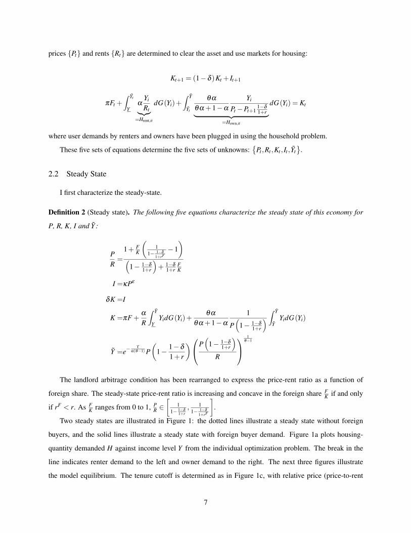
Definition 2 (Steady state). The following five equations characterize the steady state of this economy for

P, R, K, I and Y :

PR=

1+ FK

(1

1− 1−δ

1+rF−1)

(1− 1−δ

1+r

)+ 1−δ

1+rFK

I =κPε

δK =I

K =πF +α

R

∫ Y

YYidG(Yi)+

θα

θα +1−α

1

P(

1− 1−δ

1+r

) ∫ Y

YYidG(Yi)

Y =e−ϒ

α(θ−1) P(

1− 1−δ

1+ r

)P(

1− 1−δ

1+r

)R

1

θ−1

The landlord arbitrage condition has been rearranged to express the price-rent ratio as a function of

foreign share. The steady-state price-rent ratio is increasing and concave in the foreign share FK if and only

if rF < r. As FK ranges from 0 to 1, P

R ∈[

11− 1−δ

1+r, 1

1− 1−δ

1+rF

].

Two steady states are illustrated in Figure 1: the dotted lines illustrate a steady state without foreign

buyers, and the solid lines illustrate a steady state with foreign buyer demand. Figure 1a plots housing-

quantity demanded H against income level Y from the individual optimization problem. The break in the

line indicates renter demand to the left and owner demand to the right. The next three figures illustrate

the model equilibrium. The tenure cutoff is determined as in Figure 1c, with relative price (price-to-rent

7

ratio) on the Y-axis and the fraction renting (with cutoff given as Y ) on the X-axis: black lines indicate

the marginal household’s indifference condition, and the gray lines indicate relative-pricing based on tenure

shares (Greenwald et al. (2019)). Figure 1b illustrates the housing asset/investment market, with the hous-

ing supply curve in gray and the pricing equation from the net-present-value formula in black. Figure 1d

illustrates the housing use market, with the housing stock in gray and aggregated use demand (from renters,

domestic owner-occupants and foreign residents) in black.

In the special case with Ft = 0∀t and θ = 1, these equations simplify to the neoclassical q-theory.6

2.3 Impact of Additional Asset Demand

To understand the long-term impact of an increase in foreign asset demand, consider the comparative-

static analysis with a higher F .

Assumption 3 (Assumptions on parameters). The income distribution G(Y ) has a lower bound at Y = 0,

and is characterized by g′ (Y )≤ 0 everywhere. In addition,

α ≤ (1+ r)δ

r+δand θ ≥ 1−α

α

There are four parts to this assumption. First, the income distribution is characterized by a (weakly)

down-ward sloping density and hence a (weakly) concave CDF. This assumption is satisfied for exponen-

tial, Pareto and uniform distributions, for example. The second assumption puts an upper bound on the

expenditure share of housing, and realistic calibrations fall easily within that bound.

The third assumption has the most bite. A high θ implies that there is a strong sorting force, such that

small changes in relative prices do not lead to wild changes in tenure choices. In reality, tenure sorting by

income level arises from multiple mechanisms that are un-modeled here, including financing constraints.

The high θ could be rationalized on the grounds that it is a reduced-form way of capturing these multiple

mechanisms that lead to the tenure sorting, which is a robust feature of the data.

The third assumption is consistent with the CEX data. Using the CEX data and the estimation specified

in column (7) in Appendix Table 4, I get estimates of α ≈ 0.38 and θ ≈ 7.35, which satisfy the third

assumption.

Proposition 4 (Comparative static in F). In a steady-state equilibrium with a higher F: K, I and P are

higher, FK is higher, and P

R is higher. The relative level of R depends on the parameter configuration.

6The steady-state rent under this special case is R =(

δα(ΣY )κ

) 1ε+1(

1− 1−δ

1+r

) ε

ε+1 and P =

(δα(ΣY )

κ(1− 1−δ

1+r )

) 1ε+1

8

See the Appendix for the proof.

The crux of the model is to understand the various spillover effects of foreign buyers’ asset demand on

the rental market. In this partial-equilibrium model, the spillover effect onto the renter population is largely

summarized by what happens to rents, thereby affecting the real income of lower-income renters. To spell

out the four forces at play, I differentiate the user-market equation in F and rearrange in terms of d logRdF :

Λd logR

dF=π +

dYdF

Y g(Y) α

R− εK

d logPdF

−θα

θα+1−α

P(

1− 1−δ

1+r

) [d logPdF

∫ Y

YYidG(Yi)+

dYdF

Y g(Y)]

where Λ≡ α

R

∫ YY YidG(Yi)> 0.

First, the foreign buyers have some usage demand (i.e. a fraction π of them buy the housing as primary

residence or vacation home). Second, there are more renters and average renter income goes up. Third, the

asset demand spurs investment and there is more housing supply – this is the main neoclassical q-theory

force and is stronger for higher supply elasticity ε . Fourth, there are fewer owners (extensive margin), and

owners who stay owners also demand less housing (intensive margin) because the cost of housing has gone

up. The last two forces will take more time to manifest. Of these four, the first two forces raise rent, while

the last two lower it, making the net effect ambiguous.

Given the partial-equilibrium nature, there are missing forces. For example, higher house price may lead

existing homeowners to spend more due to a wealth effect. This increases income, for those working in the

local non-tradable sector (Mian and Sufi (2014)), raising the level of yi in the rental demand equation.

The dynamics of the impact are shown for a calibrated example in Figure 2. The first three figures plot

the following model quantities against time: housing stock (Figure 2a), house price per unit of housing

(Figure 2b),and the fraction of domestic households that rent (Figure 2c).

In addition to rent, user cost also changes. User cost for owners (or flow benefit) is defined as Pt −1−δ

1+r Pt+1 in period t (required return plus depreciation minus capital gain). The domestic residents’ average

user-cost is defined as the quantity-weighted average of the user costs:

∫user costit

Hit∫Hit

=α

(∫ YtY YidG(Yi)

)+ θα

θα+1−α

(∫ YYt

YidG(Yi))

Kt −πFt

which is affected by three things: total supply Kt , foreign buyers’ residential demand πFt , and the tenure

shares Yt . With π = 0, user cost is unambiguously lower under Proposition 4. Rent, owners’ user cost and

9

the average user cost for the same calibrated example are plotted in Figure 2d.

Importantly, rent adjusts to the new steady-state value immediately. This is in contrast with the slow

adjustment of the average user cost as well as the adjustment of rent in a classical q-theory framework, in

which rent adjusts only as supply expands. In this model, owner-occupied homes are quickly converted to

rental units, allowing for the rent to adjust immediately. This quick adjustment will be found in the empirical

analysis of Chinese buyers in the empirical section later.

2.4 Mean and Median Welfare

How does the foreign buyers’ housing-market impact translate into welfare impact for domestic house-

holds over the income distribution? Given the stylized model in this paper, the welfare discussions are

suggestive but not comprehensive. In particular, much of the welfare impact on owners who remain owners

depends on the welfare impact of housing-wealth shock more generally (Berger et al. (2017)). In particular,

the model abstracts away from collateral constraints, which make housing-wealth shocks more welfare-

improving for homeowners by relaxing the constraints (Mian and Sufi (2011); Kaplan and Violante (2014)).

This is an important caveat and will be discussed more in detail below.

Proposition 5 (Steady-state welfare gradient). In the new steady state with foreign buyers relative to the

one without, the welfare difference is weakly decreasing in the income level.

See the Appendix for the proof. The result is intuitive given that price-to-rent ratio is higher in the new

steady state per Proposition 4. For an illustration, see the solid black line in Figure 2e. The shape is also

intuitive: the switchers’ welfare change is lower than that of original renters, because the welfare loss from

choosing renting over owning is increasing in income level, but by revealed preference, their welfare change

is higher than owners who stay owners.

The overall welfare impact of foreign-buyer entry is a combination of this long-term impact and the

initial impact of the price increase, which delivers a positive wealth shock to those who own housing. In

decomposing housing wealth shocks, this has been called the endowment effect (Berger et al. (2017)). The

net present value (NPV) that combines the impact of the positive endowment effect and the ongoing higher

cost of living determines the overall welfare impact.

A numerical example of the NPV welfare impact – in an example calibration with rent decrease – is

shown in Figure 2e. The small red dots indicate the initial news shock that delivers positive endowment

effect on owners, expressed as the ratio of the new utility over an economy that did not see foreign-buyer

entry, plotted against the income of a domestic household. The black dashed and solid lines are the relative

10

welfare at t = 1 (event time) and the new steady state. The black circles indicate the overall NPV ratio.

It shows that the household with the highest welfare gain is the marginal owner in the original economy,

who received the endowment shock and did not mind renting too much. This last implication applies more

broadly in the model.

In the static model here, the gain from the price jump is consumed, rather than spread out over multiple

periods. This is a possible limitation of the static modeling of the household problem. Nonetheless, the

broader insight that the endowment effect is dominated by the price rise (e.g. income effect) for owners

is robust, as long as δ > 0 (Berger et al. (2017)). The price gain applies to the current housing stock

owned, but that stock depreciates over time and hence cannot guarantee the same amounting of housing

over time. To make up for depreciation, the payments are now more expensive. The key is that depreciation

or homeowners’ cost of maintenance scales with price P. This may be due to several reasons: One example

is homeowner association (HOA) fee, which tends to be higher when an area becomes more expensive;

another is property tax, which scales with the property value albeit with lags and caps in the short run.

To illustrate with a stark example, take a sufficiently high-income household who was a homeowner

and stays a homeowner. Nothing changes, except they now pay higher HOA fees and property taxes. They

could sell the house to rent or move out, capturing the gain. That choice is modeled in, but it is not taken.

Ownership has gains that are a luxury, so such a high-income household bears a larger cost to sell and

capture the price gain. For example, there may be a preference to be in an exclusive suburb, which would

be too costly to give up on for high-income households. The θ in the model captures this and other forces

that make giving up homeownership costly, especially for higher-income households.

Given this cross-sectional welfare impact, it is possible to contrast the mean welfare impact against

the median impact, presented as the time series of flow utility ratio against no-foreign-buyer economy in

Figure 2f. In this numerical example, the average cost of housing decreases driven by the large rent decrease

(Figure 2d) so the aggregate welfare is higher with the foreign-buyer demand. Yet, because homeowners are

the majority of the population, the median welfare is lower due to the higher cost of living for homeowners.

More broadly, welfare gains are concentrated among the minority renters, so even despite the aggregate

welfare gain, median voter theorem implies political or social response to the foreign-buyer shock would be

negative. For the starkest example, take the case when π = 0, under which the average user cost definitely

goes down; as long as Y0 < 0.5 and Y1 < 0.5, the median person (either by income or by welfare impact) will

oppose. The negative response would be more pronounced if voice or influence were increasing in income.

The divergence between mean and median welfare is not the case in many dense cities (e.g. Chicago at 45%

homeownership), but those areas often have a low elasticity of housing supply, so the welfare gain itself

11

might be small or negative.

The income-gradient of welfare impact analyzed here is limited: With credit constraints, the rise in house

prices can be welfare-enhancing for constrained homeowners (Mian and Sufi (2011); Kaplan and Violante

(2014); Berger et al. (2017)).7 More broadly, the literature on housing wealth has identified many ways in

which a rise in house price can increase – rather than decrease – real income. Some of them are modeled

here, most notably the ability to sell the house to capitalize on the capital gain while moving to the rental

option. If homeowners were credit constrained, the higher house price, while raising the cost of living, can

still raise welfare by relaxing collateral constraints. Such welfare gain among homeowners could counteract

some of the implications discussed here. Nonetheless, the welfare consequence still holds for homeowners

who own only their primary residence, has sufficient liquidity buffer and has a strong preference for owner-

occupied housing.

The welfare impact is testable with survey elicitation of reactions to foreign buyers, institutional in-

vestors and incoming residents in gentrifying neighborhoods, which can then be correlated with income,

tenure and liquidity-constraint proxies.

3 Measuring Ownership of US Housing by Residents of China

I study the empirical impact of buyer entry on local housing markets in the concentrated episode of

Chinese foreign buyer entry in 2010-2019. Given the large magnitude – estimated at roughly $200 billion

of residential purchases in a decade – the episode is of independent interest as well. I begin by proposing a

methodology to measure Chinese ownership in US housing.

3.1 Data and Measurement

Information on foreign direct holdings of US real estate is not readily available. I construct zip-code-

level panel data on Chinese holdings of real estate properties using deed records from CoreLogic. I use last

names on deed records as the main search criterion to identify Chinese owners and buyers.

“Chinese buyers” can encompass many types of buyers. I begin the measurement exercise by concep-

tually defining the type of buyers I want to capture. Most importantly, they are not local residents, and in

particular they purchase properties using wealth from abroad. It also matters that the buyers have a higher

7Many empirical studies focus on the impact of house-price increase on consumption. However, consumption response tohousing wealth shock is not equivalent to the welfare impact. Under a Cobb-Douglas aggregator between housing and non-durableconsumption for example, consumption remains unchanged even if house price rises and welfare falls. If there are in addition someconstrained households who then increase consumption, it is possible to have consumption go up but average welfare still go downamong homeowners.

12

willingness-to-pay via a higher effective discount factor.8 The property purchased could be used for mul-

tiple purposes, e.g., as primary residence for a family member (for example, properties bought by parents

residing in China for their children residing temporarily in the US to attend college), as vacation home to be

left vacant when not in use, and as an investment home to be rented out. The key delineation is the source

of capital, and the various restrictions on buyer names below will be imperfect ways to get at this class of

buyers.

The 100 most popular Chinese surnames account for 85% of China’s population.9 See Online Appendix

Table A.1 for the list of the 100 surnames in 2007, with the Mandarin Pinyin romanization. I use four

common romanization schemes under two dialects to identify Chinese last names: Pinyin and Wade for

Mandarin, and Jyutping and Hong Kong Government Cantonese Romanisation (HK) for Cantonese. For

example, for the third most common last name, the possible romanizations are Zhang (Pinyin), Chang

(Wade), Zoeng (Jyutping) and Cheung (HK). Other romanizations (e.g. Cheong and Chong) are excluded.

If any of the individual owners of a property has one of the 100 last names, I classify that property as

belonging to a Chinese buyer. In the 2012-2013 assessor cross-section of the CoreLogic deed records, the

actual frequency of the 100 last names is ranked in Online Appendix Figure A.5 against the frequency rank

in China’s population as of 2007. The downside of this measure is that it also captures Chinese Americans

(roughly 1% of the US population) and non-Chinese last names with the same alphabetization (e.g. Long).

To exclude both Chinese Americans and non-Chinese individuals with the same surname alphabetiza-

tion, I exclude individual buyers with non-Chinese first names. Information on origin of first names comes

from a website “Behind the Name: The etymology and history of first names” (https://www.behindthename.com/).

For example, searching for the Chinese romanization of my first name (“Zheng”) shows that the name is

Chinese, while searching for my unofficial English name (“Max”) shows that the name is German, English,

Swedish, Norwegian, Danish or Dutch. In all of the measures of Chinese buyers, I exclude buyers with first

names that are identifiably non-Chinese.

I construct two main measures of Chinese buyers. The “broad measure” includes all individual and

institutional buyers with a Chinese surname, and without a non-Chinese first name. Given these restrictions,

most institutional buyers I include are trusts. The “narrow measure” further imposes that there are no loans

on the deed record, as Chinese buyers disproportionately engage in all-cash transactions (71% of transactions

according to Yun et al. (2017)). Lastly, for comparison I separately measure buyers with Chinese surnames

8As mentioned above, Chinese buyers likely have higher average wealth, have limited domestic investment opportunities due topolitical risk, and have consumption process less correlated with the US geographies they enter.

9LaFraniere, Sharon. “Name not on our list? Change it, China says.” The New York Times. April 20, 2009. As the articlepoints out, Chinese word for “the people” is bai xìng. Translated literally, it means “hundred surnames.” Top 100 surnames accountfor only 16.4% of the population in the US by contrast (Word et al. (2008)).

13

and English first names as a rough proxy for Chinese American buyers. For each of these measures, the

main specification of the variable is defined as

share≡ 10.85

# of units held by groupzt

total # of unitsz

for zip code z in year t. I used the 100 most popular Chinese surnames to identify Chinese owners. Since

those surnames account for roughly 85% of the Chinese population in China, I scale up the measured

Chinese share by 10.85 . I also use alternative specifications where I use total square footage or total number

of bedrooms instead of number of units.

As for the sample of housing data, I use CoreLogic deed and tax records from 1,116 jurisdictions cov-

ering the counties shown in Online Appendix Figure A.3, to have a consistent and comprehensive coverage

for 2000-2015. Those counties cover roughly 60% of the US population.

If I am solely interested in measuring Chinese international buying activity, the current methodology

omits large institutional owners. For example, “Chinese life insurance firms like Anbang have been big

buyers in New York.”10

3.2 Measured Chinese Buying Activity

The measured Chinese-owned property counts and shares are shown in Figure 3. Figure 3a plots monthly

gross purchases by Chinese buyers, using the narrow measure that further imposes all-cash financing. The

blue solid line represents the number of transactions while the red dotted line represents total values in

these transactions with magnitudes on the right axis. By both measures, purchases by Chinese buyers jumps

around 2009 and continues to increase to around 2013. Even though the methodology is conservative and

hence the plotted quantities are on the lower side, the magnitudes are large. Thousands of purchases were

made accounting for around 1 billion USD each month during the active years following 2009.

For assessing the impact of such demand on US housing markets, we care about net ownership as a proxy

for the net demand for housing assets, accounting for sales and also for the size relative to the underlying

housing markets. For that purpose, figures 3b and 3c plot the share of total residential properties owned by

those with the top 100 most populous Chinese surnames and without English first names, scaled by 0.85.

Relative to the gross flow quantities in figure 3a, figures 3b and 3c represent net stock measures.

Figure 3b is for the same narrow measure that further imposes all-cash financing, and exhibits the same

kinked increase starting around 2009. Figure 3c is for the broad measure that does not impose an absence

10Rapoza, Kenneth. “Why Washington is making it easier for rich foreigners to buy US real estate.” Forbes. February 3, 2016.

14

of mortgage: It is larger in magnitude than the narrow measure but lacks the sharp increase in 2009, instead

increasing smoothly throughout the period.

For visualizing purchase trends, the broad measure is inferior, as it may include transactions by Chinese

Americans, for example. However, for the IV estimation in this paper, the broad measure is superior. With

a broad measure, the instrument can capture only the meaningful variation due to actual Chinese buyers

that is more likely to be included fully in the broad measure. By contrast, if the observed Chinese owners

are a fraction of the actual ownership activity, then the unobserved component will be correlated with the

instrument, and hence lead to overestimates in the second-stage regression assessing the impact of Chinese

owners on local housing markets.

The average characteristics of the properties owned by Chinese owners by the broad measure are re-

ported in Table 1, for the years 2009-2014. Compared to all properties in the sample of counties, properties

purchased by Chinese buyers are more expensive and have more bedrooms, but have fewer square feet. The

majority of the purchases are for single-family homes at 68%, comparable to the overall average. Relative to

the average, Chinese buyers buy disproportionately more condominiums at 15% of total purchases, relative

to 7% for overall purchases. The deed records provide one method of approximating owner-occupation or

absentee ownership, by comparing the property address to the mailing address to which the owner decides

to mail the deed (often the residential address for domestic buyers). For Chinese buyers, this is not the most

reliable information for owner-occupation, since foreign investors – those that do not plan to live in the

properties – often use the property address as their mailing address for the deed.

The second panel of Table 1 compares the zip-code characteristics of where Chinese buyers enter against

all zip codes in the sample counties. These zip codes have higher house price, rent and incomes, in more

urban areas with lower housing supply elasticity. Relevant to the instrumentation strategy to be introduced

later, these zip codes have higher pre-existing Chinese population (5% in 2000) and have flight routes from

Chinese that are more than an hour shorter on average. They are disproportionately more likely to be in the

West Census region, and less in Midwest and South.

There is much geographical heterogeneity in the Chinese buying activity. Online Appendix Figures A.4a

and A.4b plot the broad and narrow measures, respectively, across the US. Some areas saw more dramatic

increases in Chinese ownership share.11

11In the state of Nevada (mostly Las Vegas and Reno in my sample), the fraction owned by the 100 surnames went from 0.2% in1998 to 2% in 2013, a tenfold increase. In a couple of zip codes in the outskirts of Las Vegas (89139 and 89148), the share wentfrom 0.2% and 0.3% in 1998 to 9.3% and 8.3% in 2013. Several commentators of the 2000s housing boom have pointed out thatseveral cities with elastic housing supply also experienced large price boom and bust. In particular, Nathanson and Zwick (2017)point to “anomalous cities” in “Arizona, Nevada, Florida, and inland California.” Those four states experienced 13th, first, 22ndand second highest rates of growth in Chinese share among the 50 states.

15

3.3 Validation of Chinese Buyer Measures

Given that there is no separate data set tracking buyers of US real estate who reside in China, validating

my measures is difficult. One approach is to compare actual holdings against information on potential

buyers’ interest in US places. To this end, I obtain a list of properties listed on Juwai.com. According

to the Wikipedia entry, Juwai.com is “China’s largest international property website for Chinese buyers of

overseas property... Juwai attracts 1.5 million unique visitors a month and ’is usually the first place China’s

newly rich begin their [international property] search.” If the intensity of listings on Juwai.com represents

Chinese buyers’ interest in an area in the US, then I should find those areas also have higher holdings by

Chinese owners.

One major downside of this exercise is that the Juwai.com listings were obtained in February 2017,

while the most recent real estate holdings information is in 2013. Therefore, correlations between listing

frequency and shares held will be low due to the timing mismatch. The correlations would also be lower to

the extent that listing frequency is an imperfect measure of Chinese buyers’ interest, and to the extent that

Chinese buyers’ interest does not translate to actual holdings.

Online Appendix Figure A.6a shows the geographical distribution of the ratio of number of properties

listed on Juwai.com in February 2017 to total number of properties in that zip code in 2013. Online Appendix

Figure A.6b plots the cross-sectional correlation between the Juwai.com listing intensity measure defined

above (for February 2017) with the Chinese share of properties owned in each of the year t, using the narrow

measure of ownership share. Two things are worth pointing out. First, the level of correlation is quite low but

positive. That is, Chinese owners hold bigger fraction of properties in zip codes that have more properties

listed on Juwai.com in 2017. Second, and more importantly, the correlation is rising over time, and is twice

as high in the intensive Chinese investment years of 2009-2013 as it is in earlier years.

4 Housing Market Impact

Using the estimated Chinese buying activity from the previous section, I estimate the impact of the

buyers on local housing markets. I begin by decribing the data sources for various housing-market outcomes

– house price index, rent index, building rate and owner-occupation rate – followed by simple difference-in-

difference correlations with the Chinese-ownership numbers. To get at the causal impact of Chinese demand

on these housing-market outcomes, I propose an instrumentation strategy based on the known pull factors

for Chinese buyers: flight time from China and pre-existing Chinese American presence.

16

4.1 Housing Market Data and Correlations

Housing market data are at an annual frequency for 2000-2015, and the unit of observation is a zip

code when data are available or county otherwise. Such narrow geographically aggregated or averaged data

are appropriate for measuring the equilibrium impact of foreign buyers on local housing markets. The main

housing-market data of interest are house prices, rents, investment or building rate and homeownership rates,

corresponding to the key quantities in my q-theory model. The most relevant for household welfare are the

two prices: house prices and rents.

House price data come from the Zillow Home Value Index and the CoreLogic repeat sales index. The

CoreLogic index is widely used and is constructed using a more straightforward repeat-sales methodology,

but its cross-sectional coverage is lower, with data for about 7,000 zip codes. The Zillow Home Value

Index uses Zillow’s proprietary methodology that combines repeat-sales and hedonic methodologies, and is

available for roughly 29,000 zip codes, covering most of zip codes in the US. The two are highly correlated:

In the 2000-2015 annual panel, the two have a correlation of 0.56 in logs. When zip-code and year fixed

effects are included to focus on diff-in-diff variations, the correlation implied by the within R2 rises to

0.82. Given the high correlation between the two data series and the broader coverage of the Zillow Index,

the main analysis uses the Zillow Home Value Index for house prices, and I report replications with the

CoreLogic Index in the Online Appendix.

Long panel data for rent indices are not available at the zip-code level for the study period 2000-2015. I

use two rent dices, each with limited coverage. Zillow Rent Index has zip-code level data, but only start in

2010. I also use median rents for 3-bedroom units from the US Department of Housing and Urban Develop-

ment (HUD)’s Office of Policy Development and Research website; these data span the study period, but are

available at the county level. HUD’s median rents are derived from the Census and American Community

Survey (ACS). Overall, these two data series have a panel correlation of 0.81, but once zip-code and year

fixed effects are included, the diff-in-diff variations are not correlated. Because of this low diff-in-diff cor-

relation between the two series, the data imperfections of both series and the more theoretically ambiguous

impact on rents, I report results using both data series in the main analysis.

Homeowner and renter shares come from the ACS at the county level. Building rate is obtained from

the Building Permits Survey, by mapping the FIPS place counts to corresponding counties.

I report the relationship between these housing-market variables and the measured Chinese ownership

shares in the bottom panel of Table 3. County fixed effects and year fixed effects are included because there

are clear time-invariant cross-sectional difference in zip codes (e.g. high Chinese presence and prices in

17

California) as well as aggregate trends.

The housing estimate suggests that a percentage point increase in shares of properties held by Chinese is

associated with a 0.34% increase in house prices. The average correlation with rent is positive, but splitting

the zip codes up by housing supply elasticity shows that more Chinese holdings is associated with lower

rent in areas with elastic supply, and with higher rent in areas with inelastic supply. These correlations are

consistent with the theoretical framework laid out above.

There are many reasons to be cautious in interpreting these correlations as causal impact of Chinese

buyers on local housing markets. First, the Chinese shares are measured with much measurement error,

which would bias all estimates toward zero. Second, Chinese buyers do not randomly choose where they buy

properties but make a calculated and endogenous decision. These concerns motivate the use of predictors of

Chinese buying activity in order to isolate the causal impact of Chinese buyers on local housing markets.

4.2 Instrument for Chinese Asset Demand

To establish a causal link from foreign asset demand to local housing markets, I propose an instrument

based on factors that draw Chinese buyers but are otherwise unlikely to affect the local housing markets.

The instrument interacts changes in travel times to US areas from China (driven by changes in direct flight

routes) with zip codes within those areas that have higher pre-existing Chinese American presence and are

therefore potentially more appealing to buyers from China. Flight-time changes vary mostly at the airport

level, which again varies mostly at the metropolitan-area level. For zip codes in a given metropolitan area,

the instrument can be viewed as a difference-in-difference variable, comparing local outcome before and

after flight-time changes, between high- and low-Chinese presence zip codes. I first describe each factor in

some detail and then propose the interacted instrument.

Chinese buyers value ease of access from China (Rosen et al. (2017); Yun et al. (2017)).12 Unlike

financial assets, real estate properties are heterogeneous, and hence pose an entry barrier to outsiders without

knowledge of the local housing market. This segmentation is larger for Chinese investors who must cross

the Pacific.13 When it becomes easier to fly to an area, either by having a direct flight, by making fewer

layovers or by flying fewer hours, it should lower Chinese investors’ cost of acquiring information about

a local housing market, and hence induce higher investment demand. Such a lower cost of access can be

manifested in several tangible ways for Chinese buyers. First, buyers who wish to own and rent out their

property can perform maintenance more easily. Second, for buyers of vacation homes, lower travel time

12Flight time also matters for business ownership globally (Campante and Yanagizawa-Drott (2018))13Foreign investors do hire local agents (HG.org). Higher information asymmetry still implies lower bargaining power in the

principal-agent problem between the foreign investor and her intermediary.

18

makes it easier to get there for vacations. Third, easier travel stimulates more information flow in general,

so buyers in China are more likely to learn about that area.

To measure the shortest travel time from China to various US locations, I use data on flight routes and

airport locations. Flight route data come from Department of Transportation’s Bureau of Transportation

Statistics T-100 Segment (All Carriers). The data contain origin-destination route information by airline and

plane type. I only use passenger routes flown by planes with jet engines (e.g. Boeing 747 and 777). Airport

location data come from Federal Aviation Administration’s Address of Public Use Airports.

Flight time from China can change when direct flights from China change or domestic layovers change.

The latter raises additional endogeneity concerns: More flights would open up to areas in the US attracting

more businesses, for example. To address this concern, I use historical domestic route network and route

changes that result from direct flight openings to a different city.

To be robust to the concern that flight changes may anticipate local economic conditions, I construct the

travel time instrument in the following way. I first take the domestic flight route network from 1997, the

earliest year for which I have data from the T-100 Segment data. Then, for each year, I add direct routes in

operation from any airport in mainland China to the network of 1997 domestic flights. For this network of

flights, I assume flights travel at 500 miles per hour, while layovers (i.e. passing through a node) take three

hours. To this network of flights, I add straight-line driving legs from each airport to the centroid of each zip

code. Driving legs are assumed to have distance equal to the straight-line distance between the airport and

the zip code centroid, calculated using the Haversine formula. I assume that all driving is done at 60 miles

per hour. Given this network, I calculate minimum time to each zip code centroid from anywhere in China,

year by year.

There were several direct-flight changes in the time period of the study. To list a few prominent exam-

ples, direct-flight openings include those from China to Chicago (2001), New York City (2003), Newark

(2006), Washington DC (2007), Atlanta (2008), Seattle (2009), Detroit (2010) and Honolulu (2012); direct-

flight closings include those from China to Detroit (2002) and Atlanta (2010). The frequency of direct-flight

changes generates many time series events, adding to the power of the empirical methodology. Note that I

do not include flight routes from airports in Hong Kong, Taiwan, Korea or Japan. Flights to Los Angeles,

CA and San Francisco, CA are in operation and do not change throughout sample period.

To illustrate the variations induced by the predicted flight time, Online Appendix Figure A.8a shows

the areas affected by direct flight opening to O’Hare International Airport in Chicago, IL, as an example.

The light blue areas (“open direct flight”) are affected areas in the Chicago metropolitan area, and the light

purple areas (“direct flight for some yrs”) are the list of cities above where at some point there were direct

19

flights from China. The green areas (“decrease travel time”) experienced a reduction in travel time from

China. In the yellow areas (“no change”) where minimal travel time was uanffected by direct flight opening

to Chicago, IL. Online Appendix Figure A.8b shows an analogous map for 2010, when there was a direct

route opening to Detroit, MI but a route closing to Atlanta, GA.

The other factor that draws Chinese buyers is the presence of existing Chinese population (Yun et al.

(2017)). Existing Chinese population may predict higher likelihood of Chinese purchases through multiple

channels. First, existing Chinese communities will have local amenities such as restaurants and grocery

stores that better suit Chinese buyers. Second, for those considering residence, buyers can find neighbors

who share more common language and culture. Third, the same factors that drew the existing Chinese

residents may also be attractive to incoming buyers.

In order to proxy for existing Chinese residents, I use Chinese population shares by zip code from the

2000 Census. The main specification uses a binary for having a high Chinese presence in 2000, with 1%

population share as the cutoff point. 15 % of population resides in zip codes in this category. For robustness,

I also use the Chinese population share itself.14

My identification strategy exploits the interaction of these two sources of variation, by comparing zip

codes with high pre-existing Chinese presence to those without, before and after changes in predicted flight

time from China.

4.3 IV Specification and First Stage

The actual instrument interacts the changes in travel time (actual or predicted) with a time-invariant zip-

code-level pre-existing Chinese presence measure. The first stage estimates are presented in Table 2. For

US zip code z in Core-Based Statistical Area (CBSA) m in year t, the main specification in column (3) is

Chinese sharezmt = γ0[Hours]zmt + γ1[Hours]zmt × [Has Chinese presence]z +δz +δmt +ηzmt

Column (1) is a simple cross-sectional relationship between Chinese ownership shares and flight time

from China (predicted using the 1997 domestic layout). Areas with shorter flight time as measured by lower

hours have higher Chinese ownership share. In a simpler difference-in-difference regression in column

14A previous version of this paper interacted direct-flight changes with whether the zip code has the number 4, to predict Chinesebuyer demand. In China and East Asia, the number “4” is considered unlucky because it is homophonous with the character fordeath (sì for four and sı for death in pinyin romanization). Such tetraphobia may spill over into Chinese buyers’ taste for housingassets. In Vancouver, for instance, “houses with address number ending in ’4’ are sold at a 2.2% discount” (Fortin et al. (2014)).Its predictive power derived from the correlation with existing Chinese presence. In a cross-section zip codes with the number 4 inthe last three digits of the zip code have lower Chinese American population shares (Online Appendix Figure A.9).

20

(2) with hours and pre-existing Chinese presence, with year and zip code fixed effects, we see that when

predicted hours fall, Chinese shares rise more in areas with higher pre-existing Chinese shares.

The main specification in column (3) replaces year fixed effects with year × CBSA fixed effects. This

fully controls for CBSA-level confounding factors. Housing market returns, for example, have a significant

geographic factor structure (Piazzesi and Schneider (2016)). These fixed effects absorb much of the variation

in hours itself, although not completely since airports and CBSA’s overlap incompletely. Column (4) omits

hours as a predictor.

Column (5) replaces the binary for high Chinese presence in 2000 with the Chinese population share in

2000 itself. Column (6) replaces the predicted travel time from China with the actual travel time. The results

barely change.

Column (7) uses the narrow measure of Chinese ownership share that further imposes the all-cash-

financing criterion. The instrument still robustly predicts this narrower outcome. While for measurement,

the narrower measure is more precise, for an IV regression, the broader measure is preferred. The false

positives in the broad measure will be treated as measurement error, which the IV resolves; by contrast,

the true Chinese ownership not captured by the narrow measure will be unobserved error correlated with

the narrow measure itself, leading to an upward-biased IV estimates of Chinese ownership on local housing

market outcomes.

4.4 IV Variation in Graphs

Before discussing the estimation results, I first turn to raw plots using the same IV variation in Figure 4.

These figures highlight the difference-in-difference spirit of the instrumental variable. For each zip code in

an MSA, it is first categorized by historical Chinese presence as of 2000, using 1% of population share as

the cutoff. Then, the largest flight-time change for that zip code over the same period is identified and coded

as the event year. Various outcomes variables are then averaged by event year and the Chinese-presence

binary, weighing each observation by the 2000 zip-code overall population and the size of the travel-time

change. The IV variation can be visualized as the gap between the two lines (difference between the high-

and low-Chinese-share zip codes), after the event relative to before.

The outcome variable in Figure 4a is the Chinese-owned property share. This plot could be thought

of as the first stage. Relative to the event year, we see that Chinese ownership share rises, slightly in the

low-Chinese-presence zip codes, but rapidly and gradually in the high-Chinese-presence zip codes, in the

years following the event (Figure 4b).

The next figures plot local housing-market outcomes: owner-occupation rate, house price index, con-

21

struction rate and two rent indices, one by Zillow at the zip-code level but starting in 2010 and the other by

HUD at the county level. The outcomes are broadly consistent with the model presented in this paper. Oc-

cupation rate drops immediately for the high-Chinese-presence areas, as many of the Chinese buyers bought

to convert them into rental properties.

While for identification I rely on between-zip-code variation, the local-housing-market impact is likely

to be broader than zip codes. This is most pronounced for house-price indices in Figure 4c, since buyers

arguably have higher elasticity of substitution across zip codes than residents. Because the IV variation

only exploits the difference, it is likely that the IV estimates will be biased toward zero, especially for the

house-price estimate. Nonetheless, the gap between high- and low-Chinese-present zip codes’ house prices

still rises. Construction rate gap also rises (Figure 4d).

The main outcome of interest is plotted in Figures 4e and 4f, using Zillow and HUD rent indices,

respectively. Both rent data are flawed, with the zip-code-level Zillow index beginning only in 2010 and the

longer HUD index varying only at the county-level. Nonetheless, they both show that the gap between zip

codes with and without Chinese presence widens, with rent falling where Chinese buyers enter. The rent-

drop is immediate, consistent with the model in this paper where quicker conversion of ownership properties

to rental properties enables rent to adjust faster than in a classical q-theory model where rent falls only as

overall housing supply rises.

These raw variations are consistent with the simple model, and the qualitative patterns will be confirmed

in proper estimation in the next subsection.

4.5 Estimation Results

Results from IV regressions for local housing market impact are in Table 3. For US zip code z in

Core-Based Statistical Area (CBSA) m in year t, the IV specification is

Chinese sharezmt = γ0[Hours]zmt + γ1[Hours]zmt × [Has Chinese presence]z +δz +δmt +ηzmt

Yzmt = βChinese sharezmt + γ[Hours]zmt +αz +αmt + εzmt

All regressions are weighted by zip-code population in 2000.

The estimation results confirm the graphical analysis in the previous sub-section. Higher Chinese buyer

demand raises price, spurs construction, lowers owner-occupancy rate and lowers rent. The two rent esti-

mates differ, as both data have limitations. Zillow rent index starts only in 2010 even though it is at the zip

code level. The small sample size reflects that. More problematically, the shorter sample span implies there

22

are fewer changes in flight time, i.e. variation in the instrument, hurting statistical power. On the other hand,

HUD data span the whole sample, but they are county-level data. This biases estimates toward zero, hence

leading to much smaller estimates than for the Zillow rent index.

With the HUD rent data, the longer sample and hence more flight time changes allow for heterogeneity

analysis by the elasticity of the housing supply. Splitting areas by the median Saiz (2010) elasticity of 1.5

in the sample, the last column shows that rents fell in more elastic areas. The heterogeneity in estimates is

consistent with the model in this paper. The estimate for inelastic areas is positive, also consistent with the

model.

It is worth noting that the IV estimates are much larger than the corresponding OLS correlations. The

two likely reasons are that the Chinese share variable is measured with much error and that Chinese buyers’

demand – as endogenous decision – is correlated with local conditions. It is also possible that the instrument

is not exogenous, which I address below.

One concern is that easier travel from China affects local housing markets through a different channel.

For example, tourism may increase due to easier travel, and that can increase real estate values by increas-

ing demand for hotels and other travel-related businesses. I check for this possibility by running placebo

regressions of the existence and number of hotels and bed and breakfasts using zip code-level establishment

counts from County Business Patterns. I regress present and counts of hotels and bed & breakfasts in a zip

code against the travel time from China, in Online Appendix Table A.3. The coefficients are all statistically

indistinguishable from zero.

Lastly, travel time from China should affect mostly Chinese buyers and less so Chinese Americans.

The latter effect is not zero, because Chinese buyers can arrive and invite their relatives already in the US.

Increase in Chinese landlords can also incentivize more Chinese Americans to enter those areas. Online

Appendix Figure A.10b shows that Chinese buyers respond much more strongly to travel time from China

than do Chinese Americans. The latter slope is not zero, but still much smaller than the slope for Chinese

buyers.

5 Discussion

5.1 Applications and Policy

This paper studies how buyer entry in the housing market causally impacts the rent level in the local

housing market. The empirical estimates derive from a concentrated episode of Chinese buying activity in

the US housing market in the recent decade. The model and estimates, however, apply more broadly to other

23

applications where high-wealth buyers and investors enter a new market. I discuss three specific examples,

whose importance has been rising in society and in the literature.

First and most immediate, international buyers have been prolific in other countries of origin and des-

tination as well. Chinese buyers have been buying properties in various countries, ranging from Korea to

Australia (Searcey and Bradsher (2015)), and Russian buyers have been active in the European housing

market (Moss (2014)). While details of the buyers as well as of local housing market infrastructure differ,

the general q-theory framework developed in this paper applies to these situations as well.

Second, the rental housing market in the US has seen the rise of institutional ownership, even among

single-family homes, which have traditionally been the domain of mom-and-pop landlords (Mills et al.

(2019)). This change has been eyed with concerns of monopolistic pricing in the rental housing market.

Yet, institutional owners do have the advantage that they can pool the idiosyncratic risk inherent in owning

a home as an asset. Diversification, especially when the institutional owners span multiple geographical

markets, can lower the effective discount factor, and translate to lower rent for renters. The estimates and the

framework developed in this paper can discipline the cost-benefit analysis of the changing rental landscape.

Third, in discussions surrounding neighborhood gentrification, one of the concerns is that incoming

residents with higher incomes than the existing residents will lead to higher rents for existing renters. Yet,

because housing is an investment asset that exhibits home bias, the incoming high-income residents also

bring in more asset demand, possibly above and beyond their primary residence. This benefit has not been

considered in the discussions. In addition, the consideration points to benefits of policies that make it easier

to invest in homes as a way to make gentrification more welfare-improving.

More broadly, the gentrification literature often proxies for rent using house price indices, implicitly

assuming the price-to-rent ratio is unaffected by the composition of owners. This is understandable given

the paucity of reliable rent indices. Nonetheless, this paper shows that high-income buyers’ asset demand

can lead to a divergence in rent and asset price.

While the paper focuses on housing, the mechanisms outlined apply to real assets and capital more

broadly.

The potentially welfare-enhancing impact of capital influx and the forces analyzed in this paper lead

to a few policy implications. First, particularly in response to Chinese buyers, some cities have adopted

policies to curb such investment activity and their negative consequences. One policy response may be to

tax vacancies, which can let in more landlords for rental properties, which can exert a downward pressure

on rental prices. Second, some countries impose additional taxes on investment homes to deter speculators.

It may be possible to capture the benefits of a larger buyer base by instead taxing short-term investment

24

homes only. Third, among assets investment homes pay additional taxes on the asset value in the form of

property tax.15 A broader tax base for wealth may lead to more investment into second homes, which can

lower rent and contribute positively to the housing affordability crisis. Fourth, the effect of capital influx on

aggregate welfare depends on the housing supply elasticity, which modulates the supply-expansion force.

Since supply restrictions also impact the effective supply elasticity (Gyourko and Molloy (2015)), relaxing

such restrictions can allow foreign and institutional buyers to have more positive welfare impact.

5.2 Literature Review

This paper relates to several strands in the literature. Several papers study the impact of foreign investors

on house prices: Badarinza and Ramadorai (2018); Sá (2016); Hamnett and Reades (2019) (for UK); Pavlov

and Somerville (2017) (for Canada); Cvijanovic and Spaenjers (2018) (for Paris, France); Davids and Georg

(2020) (for Cape Town, South Africa); and Been et al. (2019) (for theory). Most related to my paper are

several contemporary papers that look at the price impact of Chinese buyers in US housing markets (Gorback

and Keys (2020); Li et al. (2020)). I focus on a different question – the spillover effect onto renters – and

use a different identification strategy to get the causal impact of Chinese buyers – interacting cost of travel

with local Chinese presence.

More broadly, this paper relates to research examining second-home demand and their impact (Chinco

and Mayer (2016); Hilber and Schöni (2020); Cvijanovic et al. (2015); Haughwout et al. (2011); Suher

(2016); Favilukis and Van Nieuwerburgh (2017); and Bayer et al. (2013)). Papers in these two categories

focus on the house-price impact and the general equilibrium impact on local economy, and few papers study

the welfare impact. One exception is the structural explorations in Favilukis and Van Nieuwerburgh (2017),

which explicitly models the rent-own decision. I complement this literature by focusing on the spillover

onto renters as well as the distribution of welfare impact.

I also add to several recent empirical papers that argue for a large supply effect in housing markets:

Asquith et al. (2019); Li (2019); Mast (2019); and Pennington (2020).

This paper is complementary to the large and growing economic literature on gentrification.16 This paper

also relates to the recent literature examining the owners of the rental housing stock. In particular, larger

institutional investors have come to replace individual owners (“mom-and-pop landlords”) as the dominant

force (Mills et al. (2019): They also document correlations that higher fraction of buy-to-rent investors is

associated with higher house price level but not rent).

15Average property tax rate is 1.15% applied to the asset value (Harris et al. (2013)).16The sociological literature on gentrification is even more vast. For a recent review, see Brown-Saracino (2017)

25

Lastly, direct investment in real estate may be an alternative, under-explored channel of the savings glut

hypothesis (Bernanke et al. (2005)). The savings glut hypothesis points to the role of increased savings

by Chinese investors in lowering the US interest rate. Discussions around the hypothesis focus on the

drastic increase in US Treasury holdings by Chinese and other foreign investors over that period. Much less

attention has been paid to the role of foreign investors’ direct investment into US real estate.

5.3 Conclusion

This paper asks, when there is an influx of capital into an asset market, what are the distributional

consequences via asset and rental prices, and how do those consequences depend on asset supply elasticity?

I examined this broader theoretical question in the context of Chinese buyers’ $150 billion investment into

US residential real estate in 2010-2019.

In order to overcome the lack of official register on foreign real estate ownership, I identify Chinese

buyers in public deed records by using the top 100 common Chinese surnames. I impose further restrictions

and run several placebo tests to argue that I am indeed picking up Chinese foreign investors. The resulting

data set shows that indeed there was a large increase in assets held by those with Chinese surnames, and that

the impact was heterogeneous across the US.

To get at the causal impact of Chinese asset demand on local housing markets, I proposed an instrument

that interacts two forces that affect where Chinese buyers were more likely to go. The first is travel time

changes due to direct flight route openings from China, as a way to shift Chinese buyers’ cost of traveling

to the US. The second force is existing Chinese American presence to reduce cultural and informational

barriers.

The resulting IV estimates show that Chinese investment demand, proxied for using actual Chinese pur-

chases, had a causal impact in increasing house prices. While the effect on rent is theoretically ambiguous,

I find that on average Chinese asset demand lowered rent, by spurring investment as would in the q-theory

framework. This effect is concentrated in areas with high supply elasticity, where investment can easily

respond to asset demand, increasing housing stock and lowering rent.

The model and empirical estimates in this paper extend to related phenomena of foreign buyers more

broadly, increasing presence of well-diversified institutional buyers in rental housing markets, and episodes

of gentrification where high-income residents and potential buyers enter a new neighborhood. While the

q-theory force likely applies in these other settings, more research is needed to quantify its magnitude as

well as competing forces unique to each setting. More broadly, who owns an asset can have real welfare

consequences, which may be especially large in housing rental markets given housing’s importance.

26

References

Aguiar, M. and Hurst, E. (2013). Deconstructing life cycle expenditure. Journal of Political Economy,121(3):437–492.

Asquith, B., Mast, E., and Reed, D. (2019). Supply shock versus demand shock: The local effects of newhousing in low-income areas. Available at SSRN 3507532.

Badarinza, C. and Ramadorai, T. (2018). Home away from home? foreign demand and london house prices.Journal of Financial Economics, 130(3):532–555.

Battistin, E., Blundell, R., and Lewbel, A. (2009). Why is consumption more log normal than income?gibrat’s law revisited. Journal of Political Economy, 117(6):1140–1154.

Bayer, P., Geissler, C., and Roberts, J. W. (2013). Speculators and middlemen: The role of intermediariesin the housing market.

Been, V., Ellen, I. G., and O’Regan, K. (2019). Supply skepticism: Housing supply and affordability.Housing Policy Debate, 29(1):25–40.

Berger, D., Guerrieri, V., Lorenzoni, G., and Vavra, J. (2017). House prices and consumer spending. TheReview of Economic Studies, 85(3):1502–1542.

Bernanke, B. S. et al. (2005). The global saving glut and the us current account deficit. Technical report.Brown-Saracino, J. (2017). Explicating divided approaches to gentrification and growing income inequality.

Annual Review of Sociology, 43:515–539.Campante, F. and Yanagizawa-Drott, D. (2018). Long-range growth: economic development in the global

network of air links. The Quarterly Journal of Economics, 133(3):1395–1458.Charles, K. K., Hurst, E., and Roussanov, N. (2009). Conspicuous consumption and race. The Quarterly

Journal of Economics, 124(2):425–467.Chinco, A. and Mayer, C. (2016). Misinformed speculators and mispricing in the housing market. The

Review of Financial Studies, 29(2):486–522.Cvijanovic, D. and Spaenjers, C. (2018). ’we’ll always have paris’: Out-of-country buyers in the housing

market. Kenan Institute of Private Enterprise Research Paper, (18-25).Cvijanovic, D., Spaenjers, C., et al. (2015). Real estate as a luxury good: Non-resident demand and property

prices in paris. HEC Paris Research Paper No. FiN-2015-1073.Davids, A. and Georg, C.-P. (2020). The cape of good homes: exchange rate depreciations, foreign demand

and house prices. Foreign Demand and House Prices (May 30, 2020).Davis, M. A. and Ortalo-Magné, F. (2011). Household expenditures, wages, rents. Review of Economic

Dynamics, 14(2):248–261.Favilukis, J. and Van Nieuwerburgh, S. (2017). Out-of-town home buyers and city welfare. The Journal of

Finance.Fortin, N. M., Hill, A. J., and Huang, J. (2014). Superstition in the housing market. Economic Inquiry,

52(3):974–993.Friedman, M. (1957). A theory of the consumption function. Princeton University Press.Gorback, C. S. and Keys, B. J. (2020). Global capital and local assets: House prices, quantities, and

elasticities. Technical report, National Bureau of Economic Research.Gordon, J. (2015). Soaring vancouver home prices spur anger toward foreign buyers. Reuters.Greenwald, D., Guren, A., et al. (2019). Do credit conditions move house prices? Unpublished manuscript,

MIT.Gyourko, J. and Molloy, R. (2015). Regulation and housing supply. In Handbook of regional and urban

economics, volume 5, pages 1289–1337. Elsevier.Hamnett, C. and Reades, J. (2019). Mind the gap: implications of overseas investment for regional house

price divergence in britain. Housing Studies, 34(3):388–406.Harris, B. H., Moore, B. D., and Center, U.-B. T. P. (2013). Residential property taxes in the united states.

Urban-Brookings Tax Policy Center Working Paper.Haughwout, A., Lee, D., Tracy, J. S., and Van der Klaauw, W. (2011). Real estate investors, the leverage

cycle, and the housing market crisis. FRB of New York Staff Report, (514).He, Z., Hu, M. R., Wang, Z., and Yao, V. (2020). Political uncertainty and asset valuation: Housing prices

in hong kong. Technical report, National Bureau of Economic Research.Henry de Frahan, L. and Sakong, J. (2020). Intergenerational elasticity of consumption and income.

27

Hilber, C. A. and Schöni, O. (2020). On the economic impacts of constraining second home investments.Journal of Urban Economics, page 103266.

Kaplan, G., Mitman, K., and Violante, G. L. (2017). The housing boom and bust: Model meets evidence.Technical report, National Bureau of Economic Research.

Kaplan, G. and Violante, G. L. (2014). A model of the consumption response to fiscal stimulus payments.Econometrica, 82(4):1199–1239.

Li, X. (2019). Do new housing units in your backyard raise your rents. Technical report, Working paper.Li, Z., Shen, L. S., and Zhang, C. (2020). Capital flows, asset prices, and the real economy: A" china shock"

in the us real estate market.Mari, F. (2020). A $60 billion housing grab by wall street. The New York Times. Accessed: 2021-06-10.Mast, E. (2019). The effect of new market-rate housing construction on the low-income housing market.

Upjohn Institute WP, pages 19–307.Meyer, B. D. and Sullivan, J. X. (2017). Consumption and income inequality in the us since the 1960s.

Technical report, National Bureau of Economic Research.Mian, A. and Sufi, A. (2011). House prices, home equity–based borrowing, and the us household leverage

crisis. The American Economic Review, 101(5):2132–2156.Mian, A. and Sufi, A. (2014). What explains the 2007–2009 drop in employment? Econometrica,

82(6):2197–2223.Mills, J., Molloy, R., and Zarutskie, R. (2019). Large-scale buy-to-rent investors in the single-family hous-

ing market: The emergence of a new asset class. Real Estate Economics, 47(2):399–430.Modigliani, F. and Brumberg, R. (1954). Utility analysis and the consumption function: An interpretation

of cross-section data. Franco Modigliani, 1(1):388–436.Moss, S. (2014). Why are rich russians so obsessed with buying up london property?Nathanson, C. G. and Zwick, E. (2017). Arrested development: Theory and evidence of supply-side spec-

ulation in the housing market. Technical report, National Bureau of Economic Research.Pavlov, A. and Somerville, T. (2017). Immigration, capital flows and housing prices. Real Estate Eco-

nomics.Pennington, K. (2020). Does building new housing cause displacement?: The supply and demand effects

of construction in san francisco.Piazzesi, M. and Schneider, M. (2016). Housing and macroeconomics. In Handbook of Macroeconomics,

volume 2, pages 1547–1640. Elsevier.Piazzesi, M., Schneider, M., and Tuzel, S. (2007). Housing, consumption and asset pricing. Journal of

Financial Economics, 83(3):531–569.Pristin, T. (2005). Echoes of the 80’s: Japanese return to u.s. market.Rosen, K., Margon, A., Sakamoto, R., and Taylor, J. (2017). Breaking ground: Chinese investment in us

real estate. Asia Society.Sá, F. (2016). The effect of foreign investors on local housing markets: Evidence from the uk.Saiz, A. (2010). The geographic determinants of housing supply. The Quarterly Journal of Economics,

125(3):1253–1296.Searcey, D. and Bradsher, K. (2015). Chinese cash floods u.s. real estate market.Straub, L. (2018). Consumption, savings, and the distribution of permanent income. Unpublished

manuscript, Harvard University.Suher, M. (2016). Is anybody home? the impact and taxation of non-resident buyers. Technical report,

Working Paper Furman Center New York University.US Census Bureau, D. o. C. (1996). Who owns the nation’s rental properties? Technical report.Word, D. L., Coleman, C. D., Nunziata, R., and Kominski, R. (2008). Demographic aspects of

surnames from census 2000. Unpublished manuscript, Retrieved from http://citeseerx. ist. psu.edu/viewdoc/download.

Yun, L. and Cororaton, G. (2019). Profile of international activity in u.s. residential real estate 2019.Technical report, National Association of Realtors Research Division.

Yun, L., Hale, D., and Cororaton, G. (2017). 2017 profile of international activity in u.s. residential realestate. Technical report, National Association of Realtors Research Division.

28

Figure 1: Model Steady State

These figures illustrate steady states of the model, without foreign buyers (dashed lines) and with (solidlines). Figure 1a plots housing-quantity demanded H against income level Y from the individual optimiza-tion problem. The break in the line indicates renter demand to the left and owner demand to the right.The next three figures illustrate the model equilibrium. The tenure cutoff is determined as in figure 1c,with relative price (price-to-rent ratio) on the Y-axis and the fraction renting (with cutoff given as Y ) onthe X-axis: black lines indicate the marginal household’s indifference condition, and the gray lines indicaterelative-pricing based on tenure shares. Figure 1b illustrates the housing asset/investment market, with thehousing supply curve in gray and the pricing equation from the net-present-value formula in black. Figure1d illustrates the housing use market, with the housing stock in gray and aggregated use demand (fromrenters, domestic owner-occupants and foreign residents) in black.

(a) Housing quantity vs. income (b) Asset market

(c) Tenure vs. income (d) User market

29

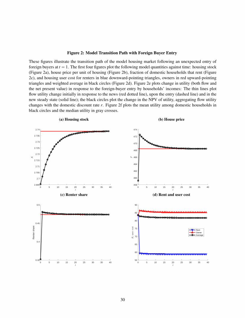
Figure 2: Model Transition Path with Foreign Buyer Entry

These figures illustrate the transition path of the model housing market following an unexpected entry offoreign buyers at t = 1. The first four figures plot the following model quantities against time: housing stock(Figure 2a), house price per unit of housing (Figure 2b), fraction of domestic households that rent (Figure2c), and housing user cost for renters in blue downward-pointing triangles, owners in red upward-pointingtriangles and weighted average in black circles (Figure 2d). Figure 2e plots change in utility (both flow andthe net present value) in response to the foreign-buyer entry by households’ incomes: The thin lines plotflow utility change initially in response to the news (red dotted line), upon the entry (dashed line) and in thenew steady state (solid line); the black circles plot the change in the NPV of utility, aggregating flow utilitychanges with the domestic discount rate r. Figure 2f plots the mean utility among domestic households inblack circles and the median utility in gray crosses.

(a) Housing stock

0 5 10 15 20 25 30 35 402.695

2.7

2.705

2.71

2.715

2.72

2.725

2.73

2.735

2.74

(b) House price

0 5 10 15 20 25 30 35 40458

460

462

464

466

468

470

472

474

(c) Renter share

0 5 10 15 20 25 30 35 400.35

0.4

0.45

0.5

Ren

ter

shar

e

(d) Rent and user cost

0 5 10 15 20 25 30 35 4055

60

65

70

75

80

85

90

RentOwnerAverage

30

Figure 2: Model Transition Path with Foreign Buyer Entry (continued)

(e) Flow and NPV utility vs. income

30 35 40 45 50 55 600.96

0.98

1

1.02

1.04

1.06

1.08

1.1

1.12

Rel

ativ

e ut

ility

Initialt=1Steady stateNPV

(f) Aggregate utility

0 5 10 15 20 25 30 35 400.96

0.98

1

1.02

1.04

1.06

1.08

1.1

Rel

ativ

e ut

ility

MeanMedian

31

Figure 3: Measured Chinese shares

These figures plot the measured real estate properties bought or owned by Chinese buyers, identified usingthe top 100 common Chinese surnames and non-English first names (“broad measure") and all-cash financ-ing in addition (“narrow measure"). Figure 3a plots monthly gross purchases, with number of properties inblue and total value in red. As opposed to this flow measure, figures 3b and 3c plot stock measure, namelythe share of total properties held by Chinese owners, using the narrow and broad measures respectively.Solid lines are shares measured by property counts, dash lines by number of bedrooms, and dotted lines bytotal square footage.

(a) Monthly gross purchases: Narrow measure

(b) Stock: Narrow measure (c) Stock: Broad measure

32

Figure 4: First stage and reduced form

These figures plot key housing market outcomes for zip codes with major pre-existing Chinese presence in2000 (maroon solid lines) and other zip codes in metropolitan areas (grey dashed lines) along with their 95%confidence intervals, in years relative to an event year in which its main flight-time reduction took place (i.e.in event time). In constructing the averages, year × zip code observations are weighed by both the 2000population of the zip code and the magnitude of the reduction in travel time from China. See main text fordetailed variable descriptions and data sources.

(a) Chinese-owned property share (first stage) (b) Owner-occupation rate

(c) House price (d) Construction rate

(e) Rent (Zillow) (f) Rent (HUD)

33

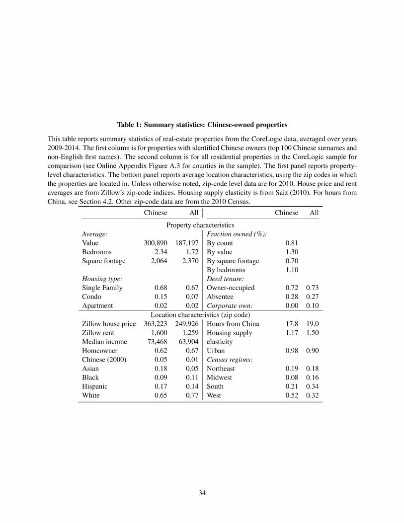
Table 1: Summary statistics: Chinese-owned properties

This table reports summary statistics of real-estate properties from the CoreLogic data, averaged over years2009-2014. The first column is for properties with identified Chinese owners (top 100 Chinese surnames andnon-English first names). The second column is for all residential properties in the CoreLogic sample forcomparison (see Online Appendix Figure A.3 for counties in the sample). The first panel reports property-level characteristics. The bottom panel reports average location characteristics, using the zip codes in whichthe properties are located in. Unless otherwise noted, zip-code level data are for 2010. House price and rentaverages are from Zillow’s zip-code indices. Housing supply elasticity is from Saiz (2010). For hours fromChina, see Section 4.2. Other zip-code data are from the 2010 Census.

Chinese All Chinese All

Property characteristicsAverage: Fraction owned (%):Value 300,890 187,197 By count 0.81Bedrooms 2.34 1.72 By value 1.30Square footage 2,064 2,370 By square footage 0.70

By bedrooms 1.10Housing type: Deed tenure:Single Family 0.68 0.67 Owner-occupied 0.72 0.73Condo 0.15 0.07 Absentee 0.28 0.27Apartment 0.02 0.02 Corporate own: 0.00 0.10

Location characteristics (zip code)Zillow house price 363,223 249,926 Hours from China 17.8 19.0Zillow rent 1,600 1,259 Housing supply 1.17 1.50Median income 73,468 63,904 elasticityHomeowner 0.62 0.67 Urban 0.98 0.90Chinese (2000) 0.05 0.01 Census regions:Asian 0.18 0.05 Northeast 0.19 0.18Black 0.09 0.11 Midwest 0.08 0.16Hispanic 0.17 0.14 South 0.21 0.34White 0.65 0.77 West 0.52 0.32

34

Table 2: First stage

This table reports the first-stage regressions of Chinese-owned property shares on minimum travel time fromChina, interacted with pre-existing Chinese presence (defined as having at least 1% Chinese population sharein 2000). For US zip code z in Core-Based Statistical Area (CBSA) m in year t, the main specification incolumn (3) is

Chinese sharezmt = γ0[Hours]zmt + γ1[Hours]zmt × [Has Chinese presence]z +δz +δmt +ηzmt

where “Hours” refers to the predicted travel time using the 1997 domestic-flight network with each year’sdirect flight from China in the main specification. Relative to this main specification, column (2) replacesthe year × CBSA fixed effects with just year fixed effects. Column (1) reports just the cross-sectionalrelationship between predicted travel time and Chinese property shares. Column (4) removes the Hoursitself as a regressor, since much of its variation is absorbed by the year × CBSA fixed effects. Column (5)uses actual Chinese population share in 2000 instead of indicator for having at least 1%. Column (6) usesthe actual travel time instead of the predicted flight time from China. Column (7) uses the narrow measureof Chinese property share (further imposing all-cash financing) as the outcome variable. All regressions areweighted by area population. Robust standard errors are reported in parentheses.

Chinese share (broad) (Narrow)

(1) (2) (3) (4) (5) (6) (7)

Hours (1997 layout) -0.269 -0.237 -0.237 -0.099× Chinese presence (0.009) (0.009) (0.009) (0.007)

Hours (1997 layout) -0.398 0.102 -0.027 -0.016 -0.025(0.007) (0.007) (0.009) (0.009) (0.003)

Hours (1997 layout) -4.749× share Chinese (0.596)

Hours (actual) -0.237× Chinese presence (0.009)

Constant 9.046 0.395 2.800 2.280 2.598 2.277 1.207(0.139) (0.125) (0.195) (0.037) (0.185) (0.037) (0.086)

Observations 175196 175196 172498 172498 172498 172498 151830Adjusted R2 0.070 0.669 0.727 0.727 0.728 0.727 0.853Partial F-stat 809 661 660 63 658 179Year FE O OZip code FE O O O O O OYear × CBSA FE O O O O O

35

Table 3: Housing Market Impact

The top panel reports instrumental-variable (IV) regressions of housing market outcomes on Chinese-ownedproperty shares, instrumented using an interaction between predicted travel times from China and pre-existing Chinese population shares in 2000, i.e. column (3) in Table 2. For US zip code z in Core-BasedStatistical Area (CBSA) m in year t, the IV specification is

Chinese sharezmt = γ0[Hours]zmt + γ1[Hours]zmt × [Has Chinese presence]z +δz +δmt +ηzmt

Yzmt = βChinese sharezmt + γ[Hours]zmt +αz +αmt + εzmt

Coefficient estimates for travel time (γ) are omitted in the table below. The outcome variables are log Zillowhouse price index (zip code), number of residential properties in log (zip code), building rate as measured bypermit count from Building Permits Survey (county), owner occupation rate from the American CommunitySurvey (county), log Zillow rent index (zip code), and log median rent from the Department of Housing andUrban Development (county). The last column separately estimates by CBSAs with high and low housingsupply elasticity, relative to median of 1.5 (Saiz (2010)). The bottom panel reports corresponding ordinaryleast squares (OLS) regressions of the same outcome variables on Chinese-owned property shares, replacingyear × CBSA fixed effects with year fixed effects. All regressions are weighted by area population. Robuststandard errors are reported in parentheses.

IV estimatesPrice # prop Build rate Owner occ Rent (Z) Rent (HUD)

Chinese share 5.301 9.466 0.430 -0.375 -1.945 -0.080(0.354) (7.346) (0.153) (0.064) (1.094) (0.045)

Chinese share 0.170(inelastic) (0.044)

Chinese share -0.651(elastic) (0.127)

Observations 157142 121542 71698 106702 42575 145193 101047Zip code FE O O O O O O OYear × CBSA FE O O O O O O O

OLS estimates

Chinese share 0.340 1.776 0.002 0.004 0.036 0.020(0.103) (0.637) (0.003) (0.002) (0.017) (0.010)

Chinese share 0.370(inelastic) (0.111)

Chinese share -0.012(elastic) (0.008)

Observations 159616 123881 74290 108300 43203 148059 101934Adjusted R2 0.961 0.266 0.761 0.986 0.971 0.955 0.949Zip code FE O O O O O O OYear FE O O O O O O O

36

A Proofs

A.1 Tenure Sorting

The additional coefficient θ affects the own-rent decision, but conditional on owning, the endogenouschoice is analogous to the case of Cobb-Douglas with elasticity θα

θα+1−αon housing. The optimal choices

are,

Hown =θα

θα +1−α

Y

P−P′ 1−δ

1+r

Hrent = αYR

Conjecture that households with income Yi > Y choose owner-occupancy. For the marginal householdwith income Y , the following utility indifference holds:

Importantly, the LHS of the indifference equation (i.e. the relative utility benefit of owning) is increasein Y , so that households with higher income will indeed sort into owning. The share spent on housing forowners is greater than for renters, i.e. θα

θα+1−α> α , which needs to be reconciled.

The pricing equation is therefore given by,Note that the constant ϒ < 0 for our parameter configuration, and so e

ϒ

θα ∈ (0,1). To see this, first notethat ϒ|θ=1 = 0 and

dϒ

dθ= α log(θα)+α−α log(θα +1−α)−θα

α

θα +1−α

< α

[log(θα +1−α)+

1θα +1−α

(−(1−α))

]+α−α log(θα +1−α)−θα

α

θα +1−α

= 0

where the inequality follows from the fact that log is a strictly concave function for positive domain (i.e.tangent is always above the function).

A.2 Comparative Static in F

In a comparative static with F ↑, cannot have both K ↓ and FK ↓. Key is to show that P and F

K respondsin the same direction. When F ↑, it is impossible to have both K ↓ and F

K ↓. Hence, either both go up (alongwith P), or they move in opposite direction. My conjecture is that they both go up, in which case I ↑ andP ↑ from asset supply, P

R ↑ from landlord valuation, Y ↑ from marginal-household indifference. R directionwould depend.I try to rule out the other two possibilities (where K and F

K move in opposite direction) by contradiction.

Case 1: If FK ↓, then K ↑ and P ↑ from supply, P

R ↓ from arbitrage and hence R ↑↑. From marginal household,d logY < d logP < d logR.Case 2: If F

K ↑ and K ↓, then P ↓ from supply, PR ↑ from arbitrage and hence R ↓↓. From marginal household,

d logY > d logP > d logR.

The first-order price effect is straight-forward and contrary to the two postulated sign changes. The keyis to show that the endogenous, extensive-margin response of Y does not undo the direct effect, but justmitigates it (which it should).

37

Leibniz rule with respect to F for the user-market equation:

dKdF

(1−π

FK

)︸ ︷︷ ︸

>0

−πKd(F

K

)dF

=− α

Rd logR

dF

∫ Y

YYidG(Yi)−

θα

θα +1−α

1

P(

1− 1−δ

1+r

) d logPdF

∫ Y

YYidG(Yi)

+dYdF

Y g(Y) α

R− dY

dFY g(Y) θα

θα +1−α

1

P(

1− 1−δ

1+r

)=− α

Rd logR

dF

∫ Y

YYidG(Yi)−

θα

θα +1−α

1

P(

1− 1−δ

1+r

) d logPdF

∫ Y

YYidG(Yi)

+ Y 2g(Y)α

R− θα

θα +1−α

1

P(

1− 1−δ

1+r

)[ θ

θ −1d logP

dF− 1

θ −1d logR

dF

]

=d logP

dF

− θα

θα+1−α

P(

1− 1−δ

1+r

) ∫ Y

YYidG(Yi)+

θ

θ −1

α

R−

θα

θα+1−α

P(

1− 1−δ

1+r

)Y 2g

(Y)

︸ ︷︷ ︸≡ΦP

+d logR

dF

−α

R

∫ Y

YYidG(Yi)−

1θ −1

α

R−

θα

θα+1−α

P(

1− 1−δ

1+r

)Y 2g

(Y)

︸ ︷︷ ︸≡ΦR

where the second equality uses d logYdF = dY

dF1Y and d logY

dF = θ

θ−1d logP

dF − 1θ−1

d logRdF from the marginal-

household-indifference equation.Contradictions of both Case 1 and Case 2 follow if ΦP ≤ 0 and ΦR ≤ 0.

From the distributional assumption (g′ (Y )≤ 0 everywhere) and using integration by parts,∫ Y

YYidG(Yi) =

12

Y 2g(Y)− 1

2

∫ Y

YY 2

i g′ (Yi)dYi ≥12

Y 2g(Y)

This assumption along with θ ≥ 1−α

αimplies ΦR ≤ 0. r+δ

(1+r)δ ≤1α

further implies (ΦP +ΦR)≤ 0.The second part of the proposition argues that the relative level of R depends on parameter configura-

tions. Numerical examples within the assumptions suffice, using Y ∼U [0,1]. For an example where R ishigher with a higher F , consider α = 0.3, θ = 2.4, δ = 0.1, κ = 0.5, r = 0.03, ε = 0.2, rF = 0, π = 1,F0 = 0 and F1 = 2. For an example where R is lower with a higher F , consider α = 0.3, θ = 3, δ = 0.1,κ = 0.2, r = 0.1, ε = 10, rF = 0, π = 0.5, F0 = 0 and F1 = 0.5.

A.3 Special Case: Closed-form for R

At the baseline steady state with F = 0, landlord arbitrage yields R = P(

1− 1−δ

1+r

), and Hown (Yi) >

Hrent (Yi) for all Yi. The marginal-household’s indifference equation simplifies to, R = Y eϒ

α(θ−1) . With theassumption of uniform income distribution, the usage market-clearing simplifies to,

RK = α

(12

Y 2)+

θα

θα +1−α

(1− Y 2

2

)38

With an additional simplifying assumption of ε = 1, we get a simple closed-form solution for rent,

R =

√√√√√√θα

2(θα+1−α)

κ

δr+δ1+r

+ e− 2ϒ

α(θ−1)

2α(1−α)(θ−1)

θα+1−α

which equals the neoclassical benchmark when θ = 1.

A.4 Steady state welfare

For a household with income Yi at time t given optimal choices, the maximized values are:

Ut (Yi, rent) = αα (1−α)1−α (1+ r)1−α Yi

Rαt

Ut (Yi,own) =(

θα

θα +1−α

)θα( 1−α

θα +1−α

)1−α

(1+ r)1−α Y θα+1−α

i(Pt −Pt+1

1−δ

1+r

)θα

Per Proposition 4, from the old steady state to the new steady state, there are those who stay renters,those who stay owners and those who switch from owner to renter (since homeownership rate goes down).Their log utility changes are characterized by:

logUτ (Yi, rent)− logUt (Yi, rent) =−α (logRτ − logRt)

logUτ (Yi, rent)− logUt (Yi,own) =−α (logRτ − logRt)− (θ −1)α(logYi− logYt

)logUτ (Yi,own)− logUt (Yi,own) =−θα

(log(

Pτ −Pτ+11−δ

1+ r

)− log

(Pt −Pt+1

1−δ

1+ r

))From P/R increase, owner-owner welfare falls more than renter-renter. Owner-owner welfare always

falls.

B Housing and Tenure in CEX

A key feature of the model that generates the results is the preference for ownership, which generatesthat ownership is a luxury while housing consumption expenditure itself has a close-to-linear Engel curve.To assess these features of the model, I first present evidence from survey data that indeed these two featurescharacterize households’ choice of housing tenure and expenditure.

I use the Consumer Expenditure Survey (CEX) for years 1984-2016. Data processing follows standardpractices; see Henry de Frahan and Sakong (2020) for exactly how the variables were constructed. The con-sumption measure is the total flow measure, including imputed flow consumption values for both housingand vehicle for relevant owners. The housing consumption measure is rent for renters; for owners, I userent-equivalent broad measure, which includes utilities. After-tax income is used for income.

The model describes Engel curves with respect to permanent income. To that end, I instrument forhouseholds’ permanent income using their total consumption (Modigliani and Brumberg (1954); Friedman(1957); Battistin et al. (2009); Charles et al. (2009)). It is widely known that when using transitory income,housing expenditure is highly concave. Once instrumented for the permanent component, I find that therelationship becomes much closer to linear, confirming the Cobb-Douglas utility specification used in thispaper.

Figure 5 plots the key relationships. Figures 5a and 5c plot homeownership status and housing con-sumption – rent for renters and imputed user cost for owners – against log total flow consumption. Eachdot represents average values of each axis for a percentile of the consumption distribution, controlling forage, squared age and fixed effects for race, urban residence, Census regions and year of survey. These plots

39

can be thought of as the reduced form plots in an IV specification where income is instrumented for usingconsumption.

Figures 5b and 5d repeat the same exercise again sorting by consumption, but with after-tax incomeon the X-axis. These plots are loose graphical representations of the IV regression of housing tenure andhousing consumption on income, where income is instrumented for using consumption.

The first key feature is that homeownership is a luxury, as is widely known. What is notable is that evenin the top of the permanent-income distribution, with the exception of the top 5%, homeownership rate doesnot reach 100%. Homeownership is increasing in income for most of the permanent-income distribution.This is important because what generates that homeownership is a luxury relies on preference for livingin owner-occupied housing. An alternative and complementary mechanism for generating luxury home-ownership is credit constraints on buying a home. What is notable here is that if the sole mechanism wereborrowing constraints, we would expect the concavity to kick in lower in the permanent-income distribu-tion. By contrast, the relationship is less concave and quite steep for a large segment of the distribution,suggesting that whatever mechanism that generates luxury homeownership operates throughout most of thepermanent-income distribution.

Moving onto housing consumption, two features are notable. First is that log-on-log relationship be-tween housing and total consumption is linear, and with a slope close to one. Second, the Engel curve forowners is shifted up relative to renters in a parallel shift. Both features are implications of the preferencefor homeownership and housing consumption as modeled in this paper.

The corresponding regression results in Table 4. First two columns present regressions of homeown-ership indicators on log consumption flow, with and without controls for age, year of study, urban status,Census region and race.

The next six columns regress housing consumption on log total consumption, a homeowner dummyand the interaction between the two. The first row is the Engel curve for renters, with a log-on-log slopefairly close to one. The second column confirms that the Engel curve slope is not different between rentersand owners. Another important estimate is the coefficient on the homeowner dummy, which corresponds tothe parallel upward shift in the Engel curve as in Figures 5c and 5d. With the exception of column 3 withno controls, there is 8-17% higher expenditure on housing for owners than for renters, conditional on totalconsumption.

Columns 7 and 8 replicate the full specification of column 6, but with after-tax income as the mainEngel-curve regressor instead of consumption. Column 7 instruments for income using consumption, andis the main specification of the permanent-income regression. Column 8 presents the raw OLS regressionof housing consumption on income. The coefficient on log income again finds an Engel curve close toone in column 7, at 0.809 for renters and 0.751 for owners. By contrast, using also the transitory-incomevariation in column 8, the slope is much smaller, recovering the familiar concavity in housing Engel curvewhen contemporary income is used instead of some measure of the permanent income. The last column isthe first stage, regressing after-tax income on consumption.

Together, these results show three things. First, homeownership is a luxury, not just in the lower end ofthe permanent-income distribution, but throughout. Second, housing consumption has a log-on-log slopeon total consumption close to one and hence has close to unit income elasticity when permanent incomeis used. Third, throughout the distribution, homeowners spend about 8-17% more on housing than renters,conditional on permanent income. All three results are implications of the simple model, which are borneout robustly in consumption data.

40

Figure 5: Housing and Tenure in CEX

These figures plot tenure choice and housing expenditure by tenure status using the Consumer ExpenditureSurvey (CEX) data, as bin scatters. Each dot represents the averages constructed from a percentile fromthe distribution of consumption expenditure. In the two plots on the left, the X-axis is log consumptionexpenditure (i.e. the sorting variable itself); in the two plots on the right, the X-axis is log after-tax incomewhile still sorting using consumption expenditure. In the top two plots, the Y-axis is an indicator for home-ownership as opposed to renting residence; in the bottom two plots, the Y-axis is the log of total housingconsumption (rent for renters in blue and imputed user cost for owners in red). In constructing each binscatter, each variable has been residualized by age, squared age and fixed effects for race, urban residence,Census region and year of survey.

(a) Tenure vs. consumption (b) Tenure vs. income (C sorted)

(c) Housing vs. consumption (d) Housing vs. income (C sorted)

41

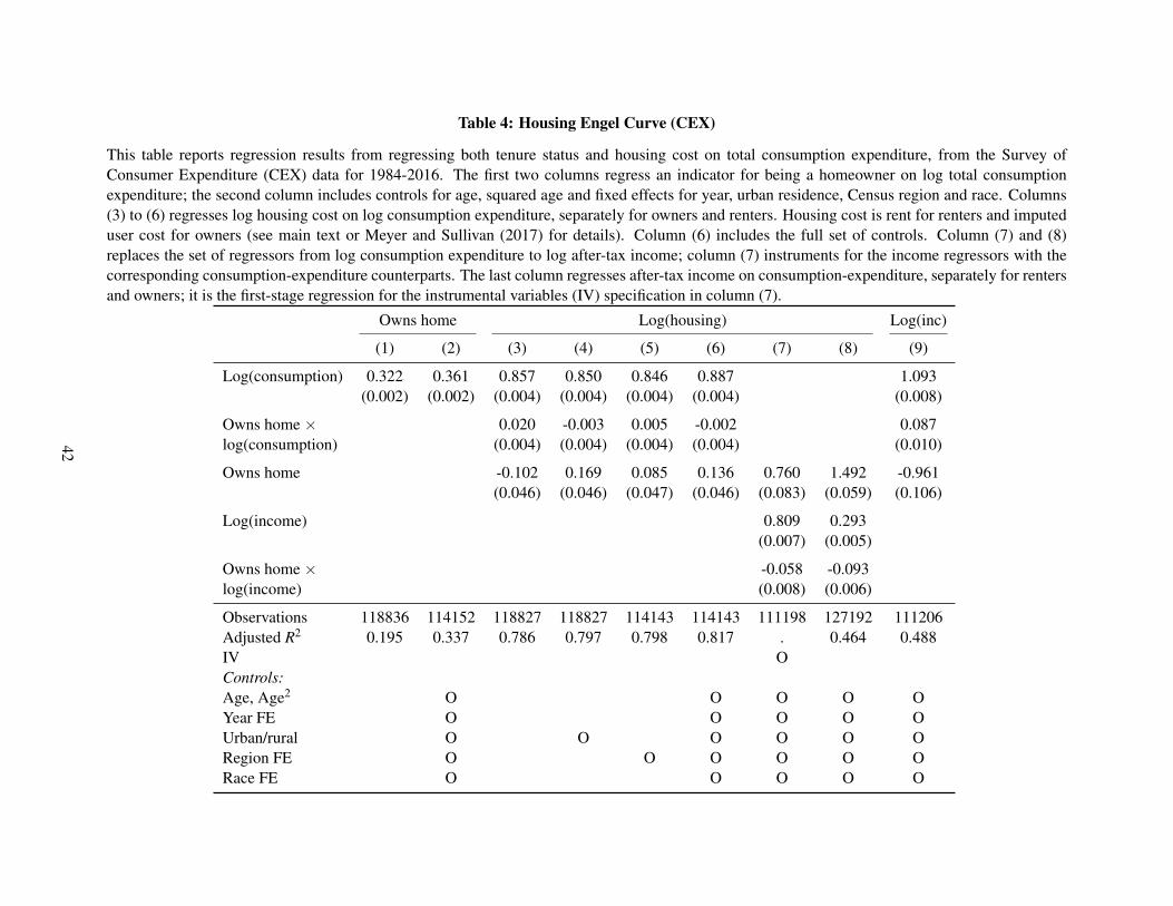
Table 4: Housing Engel Curve (CEX)

This table reports regression results from regressing both tenure status and housing cost on total consumption expenditure, from the Survey ofConsumer Expenditure (CEX) data for 1984-2016. The first two columns regress an indicator for being a homeowner on log total consumptionexpenditure; the second column includes controls for age, squared age and fixed effects for year, urban residence, Census region and race. Columns(3) to (6) regresses log housing cost on log consumption expenditure, separately for owners and renters. Housing cost is rent for renters and imputeduser cost for owners (see main text or Meyer and Sullivan (2017) for details). Column (6) includes the full set of controls. Column (7) and (8)replaces the set of regressors from log consumption expenditure to log after-tax income; column (7) instruments for the income regressors with thecorresponding consumption-expenditure counterparts. The last column regresses after-tax income on consumption-expenditure, separately for rentersand owners; it is the first-stage regression for the instrumental variables (IV) specification in column (7).

Owns home Log(housing) Log(inc)

(1) (2) (3) (4) (5) (6) (7) (8) (9)

Log(consumption) 0.322 0.361 0.857 0.850 0.846 0.887 1.093(0.002) (0.002) (0.004) (0.004) (0.004) (0.004) (0.008)

Owns home × 0.020 -0.003 0.005 -0.002 0.087log(consumption) (0.004) (0.004) (0.004) (0.004) (0.010)

Owns home -0.102 0.169 0.085 0.136 0.760 1.492 -0.961(0.046) (0.046) (0.047) (0.046) (0.083) (0.059) (0.106)

Log(income) 0.809 0.293(0.007) (0.005)

Owns home × -0.058 -0.093log(income) (0.008) (0.006)

Observations 118836 114152 118827 118827 114143 114143 111198 127192 111206Adjusted R2 0.195 0.337 0.786 0.797 0.798 0.817 . 0.464 0.488IV OControls:Age, Age2 O O O O OYear FE O O O O OUrban/rural O O O O O ORegion FE O O O O O ORace FE O O O O O

42