NASA AVRADCOMTechnical Paper 1287 Technical Report 78-18

Effect of Geometry onHydrodynamic Film Thickness

David E. Brewe, Bernard J. Hamrock,and Christopher M. Taylor

AUGUST 1978

NASA

NASA AVRADCOMTechnical Paper 1287 Technical Report 78-18

Effect of Geometry on

Hydrodynamic Film Thickness

David E. BrewePropulsion Laboratory, AVRADCOM Research and Technology LaboratoriesCleveland, Ohio

Bernard J. HamrockLewis Research CenterCleveland, Ohio

Christopher M. TaylorUniversity of LeedsLeeds, England

NASANational Aeronauticsand Space Administration

Scientific and TechnicalInformation Office

1978

SUMMARY

The influence of geometry on the isothermal hydrodynamic film separating two rigidsolids was investigated. The investigation was conducted for a conjunction fully im -mersed in lubricant (i. e., fully flooded). The effect of geometry on the film thicknesswas determined by varying the radius ratio from 1 (a ball-on-plate configuration) to 36(a ball in a conforming groove). The dimensionless film thickness was varied from 10to 10 . Pressure-viscosity effects were not considered. It was found that the minimumfilm thickness had the same speed, viscosity, and load dependence as Kapitza's classicalsolution. However, the incorporation of the Reynolds boundary conditions resulted in anadditional geometry effect. That is, the film-thickness equations can be compared asfollows:

i— \. ~* n

f Full circular film;\ Reynolds boundary conditions

Hn = 128a e(Hn) ̂ 0. 131 tan"1 ^+1. 683 )° L W 2 /J

(o. 131 tan"1 - + 1. 683^1\ 2 )\

Hn = 128a I <&. (o. 131 tan"1 2. + i 683^ P / Parabolic approximation;L W \ 2 /J I Reynolds boundary conditions

0 W 2/ s half -Sommerf eld boundaryconditions

H = 12 8 a A°u L\ Parabolic approximation;W 2/

where HQ is the dimensionless central (minimum) film thickness, a is the radiusratio Ry/Rx, e is the film -thickness effect on reduced hydrodynamic lift, and U/Wis the ratio of dimensionless speed to dimensionless load. With the Reynolds boundaryconditions the predicted load capacity is 11 to 20 percent greater than if half-Sommerfeld boundary conditions .are used. The parabolic approximation results in over-estimations of the minimum film thickness of 1. 6 and 0. 7 percent for dimensionless

-4 5minimum film thicknesses of 10 and 10, respectively.

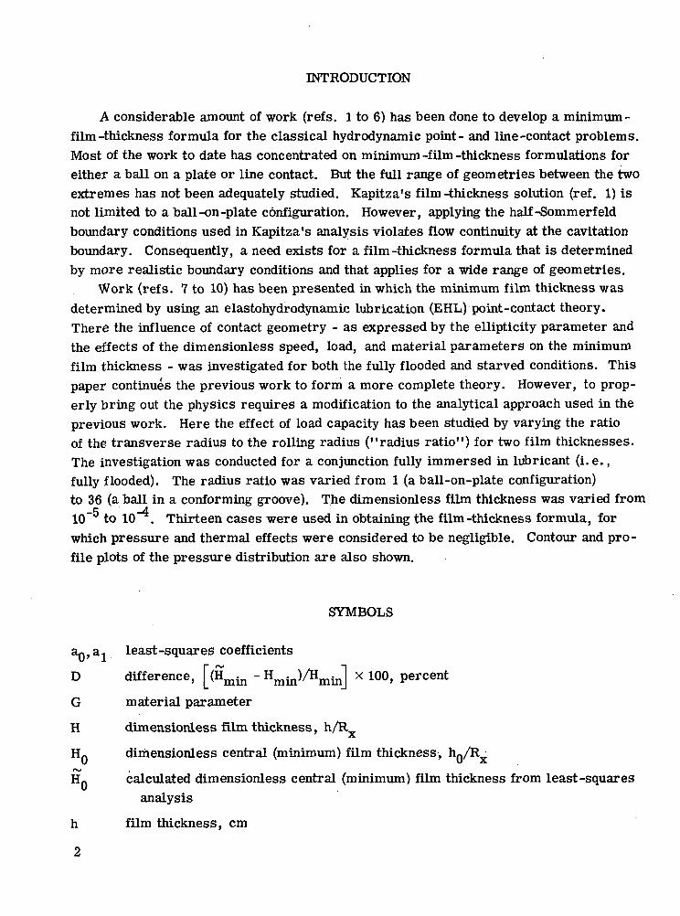
INTRODUCTION

A considerable amount of work (refs. 1 to 6) has been done to develop a minimum-film-thickness formula for the classical hydrodynamic point- and line-contact problems.Most of the work to date has concentrated on minimum -film -thickness formulations foreither a ball on a plate or line contact. But the full range of geometries between the twoextremes has not been adequately studied. Kapitza's film-thickness solution (ref. 1) isnot limited to a ball-on-plate configuration. However, applying the half-Somm erf eldboundary conditions used in Kapitza's analysis violates flow continuity at the cavitationboundary. Consequently, a need exists for a film-thickness formula that is determinedby more realistic boundary conditions and that applies for a wide range of geometries.

Work (refs. 7 to 10) has been presented in which the minimum film thickness wasdetermined by using an elastohydrodynamic lubrication (EHL) point-contact theory.There the influence of contact geometry - as expressed by the ellipticity parameter andthe effects of the dimensionless speed, load, and material parameters on the minimumfilm thickness - was investigated for both the fully flooded and starved conditions. Thispaper continues the previous work to form a more complete theory. However, to prop-erly bring out the physics requires a modification to the analytical approach used in theprevious work. Here the effect of load capacity has been studied by varying the ratioof the transverse radius to the rolling radius ("radius ratio") for two film thicknesses.The investigation was conducted for a conjunction fully immersed in lubricant (i. e.,fully flooded). The radius ratio was varied from 1 (a ball-on-plate configuration)to 36 (a ball in a conforming groove). The dimensionless film thickness was varied from10 to 10 . Thirteen cases were used in obtaining the film-thickness formula, forwhich pressure and thermal effects were considered to be negligible. Contour and pro-file plots of the pressure distribution are also shown.

SYMBOLS

a«,a1 least-squares coefficients

D difference, [(Hmin - Hmin)/Hmin] x 100, percent

G material parameter

H dimensionless film thickness, h/Rx

HO dimensionless central (minimum) film thickness, h0/Rx*>-»

Hn calculated dimensionless central (minimum) film thickness from least-squaresanalysis

h film thickness, cm

2

hg central (minimum) film thickness, cm

L reduced hydrodynamic lift

m starvation parameter (percent loss in load capacity)

N direction normal to boundary

P dimensionless pressure, pR /vwuo

p pressure, N/cm

Q solution to homogeneous Reynolds equation

R effective radius of curvature, cm

r radius of curvature, cm

S separation due to geometry of solids, cm

U/W ratio of dimensionless speed to dimensionless load

u average surface velocity in x-direction (UA +Ug)/2, cm/sec

w load capacity, N

X dimensionless coordinate, x/RA,

x coordinate along rolling direction, cm

Y dimensionless coordinate, y/R_A

y coordinate transverse to rolling direction, cm

a radius ratio, R,7/R_.y x

e film-thickness effect on reduced hydrodynamic lift

TJ dimensionless coordinate, Y/t/2oH0o

VQ fluid viscosity at standard temperature and pressure, N- sec/cm

cp Archard-Cowking side-leakage factor, [l + (2/3a)]~

X dimensionless coordinate, X/ 1/2HQ

Subscripts:

A solid A

B solid B

E entrance, or inlet

x,y coordinate direction

0 center of contact

°° infinite domain

THEORETICAL FORMULATION

Solution for Central Film Thickness

The thickness of a hydrodynamic film between two rigid bodies in rolling contact canbe written as the sum of two terms; that is,

h = h0 + S(x,y) (1)

where

hQ central (also minimum) film thickness due to hydrodynamic effects

S(x,y) separation due to geometry of solids

The separation of two rigid solids (fig. l(a)) in which the principal axes of inertia of thetwo bodies are parallel can be written as

where

-fix7*2

SBx = rBx

SBy = rBy ' VrBy '

A simplifying transformation can be effected by summing the curvatures in the x = 0and y = 0 planes. In terms of the effective radius of curvature,

1 _ 1 , 1Rx rAx rBx

Ry rAy rBy

The resulting equivalent system is shown in figure l(b). The separation in terms of thecoordinates and the effective radius of curvature is

S(x,y) = Rx - - x + Ry - - y (2)

Thus equation (1) is completely determined when the hydrodynamic effects on the centralfilm thickness are known. These effects can be determined by applying the conservationequations for an incompressible Newtonian fluid under laminar, isothermal, isoviscous,steady -state conditions. The following Reynolds equation is obtained:

J_/h39P\ + A/h39P\ = l2l,nu^ax \ ax/ ay \ ay/ ax

(3)

where u represents the average surface velocity between the two solids along the rollingdirection. It is convenient to nondimensionalize with respect to the effective rolling ra-dius; that is,

Rx R R(4)

also

"0" R

where a denotes the "radius ratio. " In terms of these dimensionless variables theReynolds equation becomes

ax ax aY 3Y ax(5)

The film -thickness equation in dimensionless form is

H = En + 1 - \ 1 - X" + ot 1 - 11- (6)

n <\

For situations in which X « 1, and (Y/or) « 1, it is convenient to expand H in atwo-dimensional Taylor series to give

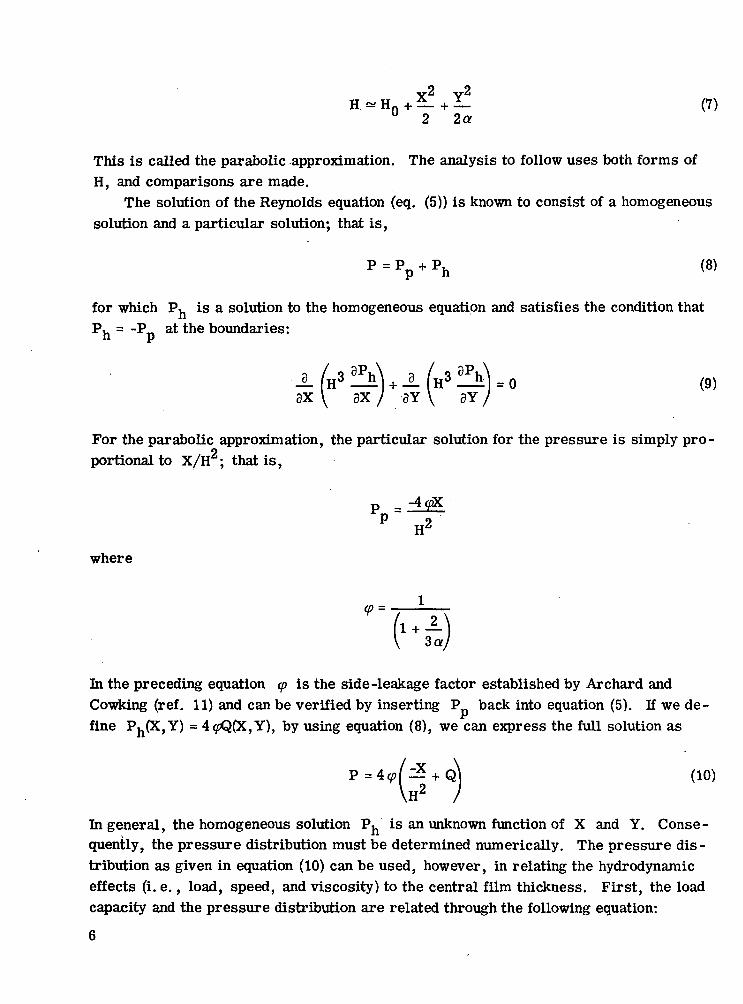
H. « Hn + - + JL (7)U 2 2tf

This is called the parabolic .approximation. The analysis to follow uses both forms ofH, and comparisons are made.

The solution of the Reynolds equation (eq. (5)) is known to consist of a homogeneoussolution and a particular solution; that is,

P = Pp + Ph (8)

for which Ph is a solution to the homogeneous equation and satisfies the condition thatPh = -P at the boundaries:

a / S 9Ph\ a / S 9Ph\_L (H3 -Jl + -1 H3 —£. = 0 (9)3X \ 3X / 9Y V 3Y /

For the parabolic approximation, the particular solution for the pressure is simply pro-portional to X/H2; that is,

P ,P

where

In the preceding equation q> is the side-leakage factor established by Archard andCowking (ref. 11) and can be verified by inserting P back into equation (5). If we de-fine P,(X,Y) = 4(pQ(X,Y), by using equation (8), we can express the full solution as

(10)

In general, the homogeneous solution P, is an unknown function of X and Y. Conse-quently, the pressure distribution must be determined numerically. The pressure dis-tribution as given in equation (10) can be used, however, in relating the hydrodynamiceffects (i. e., load, speed, and viscosity) to the central film thickness. First, the loadcapacity and the pressure distribution are related through the following equation:

w = f f p dx dy (ID

or in dimensionless form (vising eq. (4))

w = dXdY

Substituting equation (10) into this expression gives

_ + Q \ d X d Y

For the parabolic film assumption, the central film thickness can be isolated from theintegrand by defining the following transformation:

Y =

If we assume the homogeneous solution to transform in the same manner as the particular solution, we obtain

w = -x Q(x,r?)(1 + X +

(12)

Kapitza refers to this integral as the reduced hydrodynamic lift L. Thus,

L = (13)

The reduced hydrodynamic lift in Kapitza's analysis was determined to be n/2 by as-suming Q = 0 and integrating over the half-space of positive pressures. For Reynoldsboundary conditions, the limits depend on the shape of the cavitation boundary and hencethe geometry. Consequently, we seek an additional geometry effect in Kapitza's solution.Equation (12) enables us to determine the central (minimum) film thickness as a functionof the load, speed, geometry, and fluid viscosity; that is,

The ratio of dimensionless speed to dimensionless load may be defined as

W w

and equation (14) becomes

HQ = 128a feA (16)U V W /

For the parabolic approximation, we need to determine L only as a function of thegeometry; that is,

[x2 « (1/2HQ)L = L(a) if 4

|/ « (1/2H0)

This will be determined numerically. If, on the other hand, the film thickness is largeenough that these inequalities cannot be satisfied throughout most of the domain, theexact film-thickness equation (eq. (6)) must be used. The integrand of equation (13) thusbecomes a function of the central film thickness. Consequently, L = L(a,Hn), resultingin a transcendental equation for HQ.

Boundary Conditions

Earlier theories (ref. 12) assumed the pressure to be ambient or zero at the pointof closest approach. This resulted in an antisymmetric solution with respect to X(fig. 2(a)). In actuality, the lubricant is unable to sustain the negative pressures pre-dicted by the full solution. A simple approach taken by Kapitza (ref. 1) was to ignorethe negative pressures, that is, to employ the half-Somm erf eld boundary conditions.This solution (fig. 2(b)) has been used to get a reasonable estimate for the load capacity.However, Kapitza's solution does not satisfy continuity conditions at the exit (cavitation)boundary; that is, the pressure gradient normal to the cavitation boundary must be zero.To insist on P = (3P/3N) =0 at X = 0 would be overspecifying the problem mathe-matically. However, we can insist on P = (3P/3N) = 0 at the cavitation boundary

8

(i. e., Reynolds boundary conditions). The general solution will then appear as in fig-ure 2(c). For film thicknesses of about 10 to 10 centimeter, Dowson (ref. 13) hasshown that other boundary requirements are needed. For that investigation, the cav-itation boundary as determined by the Reynolds boundary conditions did not coincide withthe cavitation boundary observed experimentally. Taylor (ref. 14) has summarized sev-eral of the boundary requirements that have evolved as a result of Dowson's work.Among the boundary requirements discussed, the Reynolds boundary conditions werechosen as the most appropriate for the conditions of load and speed in this investigation.

NUMERICAL ANALYSIS

A pressure distribution satisfying the Reynolds equation (eq. (3)) was determinednumerically for a given speed, viscosity, geometry, and film .thickness. The numericalsolution was achieved by using the Gauss-Seidel iterative method with overrelaxation.The parameter $ = PH ' (ref. 15) was introduced to help the relaxation process. Acomputer program is given in the appendix.

Nodal Structure

A variable-mesh nodal structure (fig. 3) was used to provide close spacing in andaround the pressure peak. This helped to minimize the errors that can occur because oflarge gradients in the high-pressure region. The grid spacing used in terms of the co-'ordinates X and Y was varied depending on anticipated pressure distribution. That is,for a very highly peaked and localized pressure distribution, the fine mesh spacing wasabout 0. 002 and the coarse mesh spacing was about 0.1. For a relatively flat pressuredistribution, the fine mesh spacing was about 0. 005 and the coarse mesh spacing wasabout 0.13.

Integration Domain

The size of the conjunction, or the integration domain, is determined so as to makethe contact fully flooded or as close to that as practical. From Dalmaz (ref. 3), a fullyflooded condition for a ball-on-plate configuration would have an inlet domain defined byXE = -1 and YE = ±1. By using the pressures from Kapitza's classical theory, the lossof load capacity resulting from using a finite inlet rather than the semi-infinite inlet usedby Kapitza can be estimated. For this purpose let m represent the percent loss in loadcapacity; that is,

oo

(17)w.

Thus as m approaches 100, the inlet becomes severely starved. If m approacheszero, the inlet is considered fully flooded. For the ball-on-plate inlet domain, m iscalculated to be 1. 61 percent. Since this represents a negligible loss in load capacity,we chose to retain the concept that a fully flooded condition exists in this case. Hence-forth, if m < 1. 61 percent, the inlet is considered as fully flooded. According to thiscriterion, the inlets for all the geometries considered in this investigation were fullyflooded (table I). The exit boundary was determined so as to allow for a fully developedcavitation boundary.

In our effort to achieve a fully flooded condition, we recognize the fact that theReynolds equation loses some of its validity at large distances from the point of minimumfilm thickness. Dowson (ref. 16) has pointed out that the errors involved in using thisequation to determine the buildup of pressure in such regions are negligible: The pre-dicted pressures are themselves so very much smaller than the effective load-carryingpressures in the region of closest approach of the solids.

Film Thickness (Parabolic Film Approximation)

Once the integration domain has been established, the film-thickness equation canbe determined numerically. First, the load capacity w is obtained from the numer-ically determined pressure distribution. Then inserting the value of w into equation (14)allows us to solve for L for various geometries.

From the data in table II, a curve fit can be effected as a function of geometry.Studying figure 4 and trying several appropriate functional forms to curve-fit the datashowed that the following equation represented the data best:

L = ax tan"1 - + aQ (18)

The values of a.-, and a., were determined to be

= 1.683'| (19)

a1 = 0.131 '

n nThe coefficient of determination r^ (ref. 17) was 0. 96 for this fit. The value of r re-flects the fit of the data to the resulting equation: 1 being a perfect fit, and 0 being the

10

worst possible fit. Inserting equation (18) into equation (16) gives for the calculated min-imum film thickness

H - = 128a I & (o. 131 tan'1 2 + 1. 683 ]] (20)IL

For comparison of the calculated film thickness with the actual input film thickness, it isconvenient to define the differences (in percent) as

<- " Hmin)

Hminx 100 (21)

The difference ranged from -2.14 to 1. 35 percent (table n).

Film Thickness (Exact Equation)

The results of using the exact film-thickness equation (eq. (6)) rather than the para-bolic approximation (eq. (7)) can be compared from the values of L given in table n.The values of L determined through the exact film-thickness analysis are always re-duced by a constant factor. Thus the dependence on geometry and film thickness for thereduced hydrodynamic lift can be separated as follows:

(22)

where L is determined by using the parabolic approximation. The values of C(HQ) aregiven in table HI. Using the parabolic approximation gives errors of 0.7 and 1. 6 percentfor film thicknesses of 10 and 10 , respectively. Although these errors are quitesmall, they would probably be larger for thicker films: As the film thickness is in-creased, the pressure distribution spreads out more evenly (e. g., fig. 5). Thus thepressures far from the point of contact, where the parabolic assumption is no longervalid, contribute more to the load capacity than if the pressure distribution had been verylocalized.

The minimum film thickness can now be written as

Hm. = 128a [i3£? (0.131 tan'1 ^+ 1. 683Yl (23)mm |_W \ 2 /]

The difference ranges from 2.00 to -2.11 percent for the exact film-thickness results intable H.

11

DISCUSSION OF RESULTS

Comparison of Theories

The minimum -film -thickness equation derived by Kapitza using half -Somm erf eldboundary conditions and assuming the parabolic approximation is

<24)

W 2

By equating equation (16) with this expression for a given speed parameter, the load ca-pacity for the two theories can be compared; that is,

(25)

The effect of the geometry on the reduced hydrodynamic lift is shown in figure 4. Thefigure shows that L, and hence the load capacity (eq. (25)), is 11 to 20 percent greaterthan that predicted by Kapitza. The least difference occurs for a ball-on-plate contact.As a is increased, the difference in load capacities approaches a constant 20 percent.The alteration of the pressure distribution due to the Reynolds boundary conditions at thecavitation boundary is responsible for this geometry effect. Figure 6 is a three-dimensional representation of a pressure distribution for a of 1. 00 and 36. 54 and il-lustrates the shape of the cavitation boundary. As a becomes large, the cavitationboundary tends to straighten out, accompanied by decreasing changes in L. The scalealong the y-axis in figure 6(a) has been magnified about 3 times to improve the resolu-tion. Consequently the differences in the shapes of the cavitation boundary are actuallysubdued as they are presented.

The two analyses resulted in the same exponent of 2 for U/W. Dalmaz(ref. 3), usingthe Reynolds boundary conditions for a ball-on-plate configuration, reported an exponentof 1.77. The lower exponent appears to be due to starvation effects resulting from theinlet condition in both the analytical and experimental results. This is illustrated moreclearly by comparing the results of applying the inlet condition of Dalmaz and the inletcondition in this study, using Kapitza's classical theory for both. A fixed oil film thick-ness at the inlet that is independent of the minimum film thickness is used in Dalmaz'sanalysis and in this study as well. But the inlet oil film thickness for the analysis of ref-erence 3 and experimental work (given in ref. 18) was roughly 5 percent of that usedhere. The effect that this has on the exponent of U/W can be seen by calculating theload capacity for two different film thicknesses while keeping the other hydrodynamic

12

-4 5variables constant. Dimensionless minimum-film-thickness values of 10 and 10 re-sult in load capacities of 0. 046 and 0.151 newton, respectively. This would yield an ex-ponent of 1.94. For thicker films (i. e., HQ = 10" ) the starvation effects become evenmore pronounced and the U/W exponent is driven down in value to 1. 84. For com-parison, from the data in table I for fully flooded conditions, we calculate the exponentto be 1. 98.

Figure 7 compares experimental data (ref. 3) taken under lightly loaded (rigid con-tacts), isoviscous conditions for pure sliding of a ball on a plate with the correspondingtheoretical results. The parameter grouping in the figure is that used by Dalmaz (ref. 3)and first introduced by Thorp and Gohar (ref. 4). The theoretical results of this paperare in excellent agreement with the data for the lower half range of HQ/WG. For thereasons previously explained, the agreement of these results with the experimental re-sults of reference 3 begins to diverge for the upper range of HQ/WG. Further, usingcomparable inlet conditions for both theory and experiment provides better agreementbetween the two for the upper range of HQ/WG, as the theoretical line of Dalmaz attestsin figure 7. For comparison, the theory by Kapitza has been included.

Contour Plots

! Isobar plots for three radius ratios (i. e., a of 25.29, 8.30, and 1.00) are shown infigure 8. The contours were generated by means of a contour-plotting subroutine anddisplayed with a Calcomp plotter. The contours belong to the family of curves defined byequation (10). The center of contact is represented by the asterisk. The pressure peakbuilds up in the entrance region, which is located to the left of the center of contact andis indicated by the +. Since the isobars in each case are evenly spaced, the pressuregradients can be easily depicted. Note that, as the radius ratio increases, the steeperpressure gradients are predominantly along the rolling direction. This implies that theamount of side leakage decreases as a increases. A decrease in side leakage is re-flected in an increase in the value of cp. For line contact y = 1 and for the largestvalue of a in this investigation (a = 36. 54) <p = 0. 998.

Pressure Profiles

Pressure profiles across the center of the conjunction and in the direction of rollingare shown in figure 9 for three radius ratios (i. e., a of 36. 54, 2. 84, and 1.00). Thepressures were generated for a constant dimensionless film thickness (HQ = 10 ). Thelocations of the pressure peaks were not altered by the fact that Reynolds boundary con-ditions were used rather than half-Somm erf eld boundary conditions. The locations of the

13

pressure peaks from reference 1 are determined by setting (3P/3X) = (3P/3Y) = 0 andsolving for X and Y as follows:

Ypk =

(26)

Equation (26) shows that the geometry does not affect the pressure peak location, as canbe verified by the numerically determined curves of figure 9. However, the magnitudeof the pressure peaks will, according to equation (10), be modulated by the Archard-Cowking side -leakage factor q>, which is a function of the geometry. The influence ofthe side -leakage factor on the pressure distribution for several geometries is shown infigure 9.

CONCLUDING REMARKS

The influence of geometry on the isothermal hydrodynamic film separating two rigidsolids was investigated. The investigation was conducted for a conjunction fully im-mersed in lubricant (i. e. , fully flooded). The effect of the geometry on the film thick-ness was determined by varying the radius ratio from 1 (a ball -on -plate configuration) to36 (a ball in a conforming groove). The dimensionless film thickness was varied from10" to 10 . Pressure -viscosity effects were not considered. It was found that the min-inum film thickness had the same speed, viscosity, and load dependence as Kapitza'sclassical solution. However, the incorporation of the Reynolds boundary conditions re-sulted in an additional geometry effect. That is, the film -thickness equations can becompared as follows:

HQ = 128* [c(H0) Jfi (o. 131 tan'1 2 + 1. w}]* J™1 circular film''L W \ 2 /J 1 Reynolds boundary conditions

HQ = I28a te (o. 131 tan'1 £ + 1. 683)? (Parabolic approximation;L W \ 2 / J [ Reynolds boundary conditions

H = 12 8 a (y® -^ (Parabolic approximation;0 \W 2) < half -Sommerfeld boundary

^conditions

14

where HQ is the dimensionless central (minimum) film thickness; a is the radius ratioR/R • e is the film -thickness effect on reduced hydrodynamic lift; <p is the Archard-y *Cowking side-leakage factor; and U/W is the ratio of dimensionless speed to dimension-less load. The Reynolds boundary conditions resulted in the predicted load capacitybeing 11 to 20 percent greater than if half -Sommerf eld boundary conditions were used.

The parabolic approximation resulted in overestimations of the minimum film thick-ness of about 1. 6 and 0.7 percent for calculated dimensionless film thicknesses of 10and 10" , respectively.

Lewis Research Center,National Aeronautics and Space Administration,

Cleveland, Ohio, May 12, 1978,505-04.

15

APPENDIX - COMPUTER PROGRAM

IMPLICIT REAL*8 (A-H,0-Z)REAL*4 XMIN,XL5N,Yi1IN,XE(60)REAL*U XG(56) ,YG(5S) , YGC(119) , DUMB (56 , 1 19 , 2)REAL*U FNjUSjWS^SjXKSfXMAX.XCENTS^CENTSREAL*U XNODFS,XDBL,YDEL,H*INS,T>!1IN,H''IAXN A M E L I S T / P . A D I U S / R A X , R A Y , R B X , R B Y , R X , R Y , U A , U B , P H E EN A M E L I S T / O U T P U T / P , P B A R , P C H E C K , S U M 3 , H O , H O B A P , U O WD I M E N S I O N P2 ( 5 6 , 5 0 , 2 )D I M E N S I O N DBS S( 3360) , VIS ( 3 3 6 0 ) , X*U (3363) , Z P P (3360) , PHI ( 3 3 6 3 )D I M E N S I O N A ( 3 3 6 0 ) , B ( 3 3 6 0 ) ,C (3360) , DLZ (3 36 0) , XL (3360) , KM ( .3350)D I M E N S I O N 3 ( 3 3 6 3 ) , H ( 3 3 6 0 ) , P P S V ( 3 3 6 0 ) , PP ( 3 3 6 3 )D I B E N S I O N I M ( 3 )COMMON/CTRINF/FN,U5,W5,GS,XMAX,XCENTS,YCENr3,YMAX,PR»1XS,XPKCOnMON/CTR/XMODFS, XDET,,YDEL,HMINS,PHIN,HHAXCOMMON/CTFINr/NC7,F

CC INPUTC

MPARA=1NVISC=0MWT=1

CC MPAPA=1: T:IE PARABOLIC APPPOX Id AT ION WILL BE USEDC NVISC=0: THE IST-VISCOns SOLHTION IS DETERHINEDC MWT=1: PARTIALLY CONVERGED SOLUTION IS STORED ON TAPEIN CASE OF CPASHC

ROSM=1.0DOIDE=1MAUR=0JENN=0ZZZ=1.0DOPI = 3. H M 5 9 2 5 5 3 5 9 D OP I V A S = a 3 5 8 . 7 D OVISO=a . 1 1D-6V A = O . O D OV B = O . O D OZ = . 6 7 D OE L P H A = 5 .827 '4 '4D-6EETA=1.68343D-5VISE=.00000030631D3ORF=1 . 9DONX=56NY=60ZD1=9.799652DOZ E 1 = 4 9 0 . 1 9 6 0 7 8 D OZ E 2 = 7 I D 1ZC1=10.000DOZC2=500.0DOJZON=10JMIN=10NCGF=10

X C E N T = 1 . 0 0 0 0Y C E N T = 1 . O O D OX N O D F = . 9 1 B < « O D OM=1

16

cC «=-1: READS IN FDRIATTED INPUT AND BYPASSES THEINITIAL CALCULATION OFC THE PRESSURE DISTR IBUTIONCC «=0: READS IN HEXADECIMAL INPUT AND BYPASSES THEINITIAL CALCUL&TI3N OFC THE PRESSURE DISTRIBUTIONCC M=+1: CALCULATES AN INITIAL GUESSC

RAX=1. 11125D3RAY=RAXRBX=1.D12RBY=-1.D12UA=10.0DO

975 CONTINUEDEL1=. 1DOMAXS2=1D2L3=. 1DOHH IN =10.0 DOHMAX=10.0PRSVMX=. 1D-18PRMX=. 1D-18

976 CONTINUEUB=UANXY=NX*NYNX1=NX-1NY1=2*NY

7.C1S = ZC1ZC2S=ZC2ZE1S=ZE1ZE2S=ZE2FN=FLOAT (IDE)IN (1) =IDEIN (2) =NYIN (3) =NCGF

CC CURVATURE SUM AND DIFFFRENCEC

RX=(1./RAX)«- (1./SBJC)RY= (1. /RAY) *• (1 . /R3Y)RHO=HX+RYGA«MA= (RX-RY) /RHD

CXCENTS=XCFNT/RXYCENTS=YCENT/EXXNODFS=XNODF/PXYM=YCENTXN=XCENT

CC DIMENSIONLESS PARA1ETEK GPOIIPI'13C

SMV = . 5* (VA*VB)

T H E T A = A T A N ( 3 f 1 V / S ? 1 ; J )EP=VISO*V*RXU=VISO*RX*V/EP

17

us=uHO=1.D-<* .PHEE=1./(1.*(2.*RY)/(3.*RX))Q1=VISE/VISOQ2=EP/19608.5268Q5=ELPHA*EPQ6=BETA*EP

I* CONTINUEZC=ZC1ZCS=ZCSA-1./ZCSB=1.0/ZD1

CC INITIAL GUESSC

IF (Pi) 5,6,75 CONTINUE

RE AD (5,700) ( ( (P2(I,J,K) ,1=1,NX),J=1,NY) ,K=1,2)700 FORMAT (8D10. 5)

GO TO 76 CONTINUE

READ (5) ((P2(I,J,1),1=1,NX),J=1,NY)READ (5) ( (P2(I, J,2) ,1=1,NX) ,J=1,NY)REWIND 8 .

7 CONTINUEXHIN=XCENTS-.20Y=O.DODO 13 J=1,NYX=O.DODO 12 1=1,NXZD=ZD1N = I*(J-1)*NXJTWIN=NY1-JIF (J.GE.JZON) ZC = ZC2YGC(J)=Y/RXYGC(JTWIN)=2.*YCEMTS-YGC(J)YMIN=YCENTS-.16YMAX = YCENTS«-. 16XG (I)=X/RXIF(YGC(JTWIN).GE.Y1AX) JMAX=JTHIN-1IF (JTWIN. EQ. JKAX .AND. XG (I) . LE. XCSNTS) LU = ?JIF (XG (I).LE. XKIN .AND. J.EQ. NY)K1 = NIF(XMIN.EQ.O.) K1=NX* (MY-1)+2IF(J.EQ.JMIN .AND. X3 (I) . LE. XCENTS) LM AX = NNVMF=NCGF+ (J-1) *SXNVMB=NVMF*NZON2IF(N.GE.NVMF .AND. N. LT. NVHB) ZD=ZE1IF(N.GE.NVMB) ZD=ZS2SQX=((X-XN)/RX)**2SQY= ( (Y-YM)/RX)**2IF (MPARA .EQ. 1) GO TO 75S (N)= (1./RX) * (1. /RY) -DSQRT((1./RX) **2-53X) -OSQRT((1./RY) **2-SQY)IF (S(N) .GT. 1./RX) S(N)=1./RXGO TO 8

75 S(N)=(RX*SQX*RY*S3Y)/2.IF (S(N) .GT. 0.5/RX) S(N)=0.5/RX

8 CONTINUEIF (M.EQ. 1) 30 TO 9PR(N)=P2(I,J,1)GO TO 10

18

9 CONTINUEPR (N)=- 1D-8

10 CONTINUEIF (J. EQ. 1 .DR. I. EQ. 1 .OR. I.EQ.NX) PR(N)=O.ODOIF(PR(N) .GT.O.) 3D TO 11PR (N)=0. DO

11 PRSV(N)=P? (N)

1213

900

CCC

.IF (PP (N) . LT. PRSV1X) GO TO 12PRSVMX=PR(N)NHOLD=NX=X+1./ZDY=Y+1./ZCXMAX=XG (NX)YDEL=Y«AX-Y1INXDEL=YDELWHITE(6,SOO) (PR(V) ,N=1,SXY)FORMAT(1H ,2HPR/70(1H ,10013. 5/))WRITE(6,1000) (S(N) ,N=1,NXY)

1000 FORMATflH ,1HS/73(1H ,10013. 5/))

FILM THICKNESS

14 CONTINUEDO 19 J=1,NYDO 18 1=1, NXN3=I+(J-1) *NXH (N3)=HO+RX*5 (N3)IF (H(N3) .GT.HMIN) 3D TO 17HMIK=H(N3)HHINS=HMINNSAVE=N3

17 CONTINUEPHI(N3)=PF (N3) *(H(N3| **1. 5)

18 CONTINUE19 CONTINUE

WRITE (6,1100) NSAVE,HMIN1100 FORMAT (1H , 6HMSA VE = ,T 1 0, 1 OX,5HHHIN=, D 16 . 5)

WRITE (6,1203) PR5VKX,NHOLD1200 PORHAT(1H ,8HPPSV»IX=,D16.5,10X,7HNHOLD=,I10(

20 CONTINUEWRITE(6, RADIUS)

CCC

CCC

INITIAL VISCDSITY AND DENSITY CALCULATION

DO 21 N=1,NXYDENS (K) = 1. «-(Q5*P8(N) ) /(1. +Q6*PR(N) )VIS(S) =Q1**(1.- (1.+Q2*PR(M» **Z)X«U(N)=DENS(N) /VI5 (N)

21 CONTINUE

RELAXATION C3EFFIENTS A ,D , C, D, L, AND M

22 CONTINUESUM'O.ODOZC=ZC1

DO 2" J=2,NYDO 23 1=2, NX1ZD=ZD1

19

N = I + ( J - 1 ) *NXN V M F = N C G F * (J-1) *NXN V M B = N V M F » N Z D N 2IF (J. GE. J Z O N ) Z F = Z C 2IF(J .GT. J Z O N ) ZC = ZC2IF ( N . G E . N V f . F . A N D . N. LT. N V M B ) Z K = Z E 1I F ( N . G T . N V M F .RtiD. N . L E . N V M B ) ZD=ZE1I F ( N . G E . N V M B ) Z E = Z E 2I F ( N . G T . N V M S ) Z D = Z E 2V1= ( ( Z E * Z D ) / ( Z E + 2D) ) **2.V 2 = ( ( Z E ) **2. ) * ( Z D - Z E ) / ( Z D + Z E )V 3 = ( Z E * * 3 . ) * ( Z E + 2 . * Z D ) / ( ( Z E * Z D ) )**2.V4= (7,D**3.)* ( 2 . * Z E * Z D ) / ( ( 2 E * Z D ) ) **2.V5= ( Z D / Z E ) **2.*V2C2D=ZC**2-ZF**2C 3 P 1 = Z C + 2 . * Z FC 3 P 2 = 2 . * Z C + Z FC F = ( Z F / ( Z C + ZF) ) **2CF1= (1./(ZCP= (ZC + ZF) **2

Z 2 = Z C / ( Z C + Z P )Z3=Z1**2ZU=Z2**2N1=N+1N2=N-1

I F ( J . E Q . N Y ) N 3 = N UY O = X M U ( N )Y 1 = X N U ( N 1 )

( N 2 )

( N 4 )Y 5 = H ( N 1 )Y6 = !l ( N 2 )Y 7 = H ( N )Y8 = H ( N 3 )Y 9 = H ( N 4 )Y 1 0 = Y 1 * D 5 Q R r ( Y 5 )Y 1 1 = Y 2 * D S Q R r ( Y 6 )Y 1 2 = Y 3 * D S Q R r ( Y 8 )Y 1 3 = Y U * D S Q S T ( Y 9 )Y 1 4 = Y O * D S Q R T ( Y 7 )

A ( N ) = V 1 * Y 2 + V 2 * Y C H V 3 * Y 1B ( N ) =za*(Y3*7,F**2C ( N ) = V t i * Y 2 - V 5 * Y O * V 1 * Y 1DLZ (N) =CF* ( Z P * C 3 PX L 1 = Y 2 * 4 . * 7 3 - ( Z D - Z E ) **2*YO+Y1*ZE**2*CF1 * ( Y3*ZF**2*CP-:2D**2* YO+ ZC**2*XL2=1.5 / (Y7**1 .5)X L 3 = Y 1 1 * ( V a * Y 6 - Y 7 * l 4 . * Z 3 * Y 5 * V l ) * Y 1 U * ( - V 5 * Y 6 * ( Z D - Z E ) **2* Y7 + Y5* V2) «•

1 Y10* ( V 1 * Y 6 - Z E * * 2 * Y 7 + V 3 * Y 5 )X L « = C F 1 * ( Y 1 2 * Z F * * 2 * ( Z F * C 3 P 2 * Y 8 - C P * Y 7 » - Y 3 * Z C * * 2 ) *

1 Y13*ZC**2* (Y3*ZF**2-CP*Y7*ZC*C3P1*Y9) *1 Y1«*C2D* ( Z F * * 2 * Y 8 + C 2 D * Y 7 - Z C * * 2 * Y 9 ) )

X L ( N ) = X L 1 * X L 2 * ( X L 3 + X L t )XM1 = 12.*U/(Y7**1.5)X M 2 = { (ZE**2. * D E N S ( N 1 ) * Y 5 / ( Z D + Z E ) + ( Z D - Z E ) * D E N S ( H ) * Y 7 -

1 ZD**2 .*DENS ( N 2 3 ) * Y 6 / ( Z D * Z E ) ) * D C O S ( T H E T A ) )X M 3 - ( Y 8 * Z F * * 2 * D E S S ( N 3 ) *C2D*DENS (N) * Y7-Y9*ZC**2*DENS ( N H ) ) * D S I N ( T H E T i )

20

XH (N) = XH1*23 CONTINUE24 CONTINUE25 SUM=O.ODO

CC RELAXATION FORMULAC

DO 30 J=2,NYHEND=0DO 29 1 = 2, NX1MN=I* (J-1) *HXMNA=HN+1nNB=MN-1HNC=NN+NX

IF(J.EQ.NY) HNC=HNDZPR(flN)=PHI(!1N) -DBF* (PHI (UN) «• (XH (UN) -ft (UN) *PHI (HNA) -B (UN) *PHI (HND)

1 -C(MN) *PHI(nNB| -DL^ (MN) *PHI (BNC) ) /XL (NN) )26 CONTINUE

IF (ZPR (NN).LE.O.) GO TO 27Y18=(ZPR(HN) -PHI (Hit)) /ZPR(MN)

GO TO 2827 ZPR(HN) =0.10-20

MEND=HEND«-1IF (BEND .E9. 1) XE(J)=XG(I)

29 PHI(MN)=ZPR(MN)29 CONTINUE30 CONTINUE31 CONTINUE

MAUR=MAUR+111 CONTINUE

IF (HHT.EQ.O) GO TO 6665 CONTINUE

WRITE (8) ((P2 (I, J,1) ,1 = 1, NX) ,J=1,NY)WRITE (8) <(P2(I, 3,2) ,1=1, NX) ,J=1,NY)REWIND 8

66 CONTINUEIF (SUB.LT.DEL3) 30 TO 311GO TO 25

C ,C VISCOSITY AMD DESSITY ITERATIONC

311 SUH2=O.ODOWRITE (6,t»83) MAUR.SUH

U80 FORHAT(1H ,5HH AUR=, 18 , 5X,6HSOH=, 18)MAUR=0PRMX=. 1D-13DO 315 J=2,NYDO 316 1=2, NX1N=I* (J-1)*NXPR(N)= (PHI(N) /(H(H) **1.5)»(ROSH-1.)*P5(N))/ROSflIF (PR(N) . LT. PRHX) GO TO 33PHMX = PE (N)PRnXS=PRMXNHOLD=N

33 CONTINUEIF(NVISC.EQ.O) 3D TO 316

21

DENSN=1.+ (Q5*PE(N) ) / ( 1. *Q6*PH (JJ) )VISN=Q1**(1.- (U + a2*PR(N)X«UN=DENSN/VISNY99=(Xf50N-X!10 (N) ) /XHUNS U M 2 = S ( I M 2 + DABS ( Y 9 9 )D B N S ( N ) = D £ N S NVIS(N)=VISN

316 XMU(N)=XMUN315 CONTINUE

MN1=1i«59 CONTINUE

JENN=JENN+1WRITE (6, 810) SOM2

810 FORMAT (1il ,5 HSUM2) , D1 C. 5)IF (SUfl2.LT.DEL1)" GD TO 32IF (MAXS2. GT. «00) 30 TO 63MAXS2=MAXS2*1GO TO 22

CC A P P L I E D N O R M A L L O A DC

32 C O N T I N U EM A X S 2 = 1W H I T E ( 6 , 4 8 1 ) J E N N

U 8 1 F O R « A T ( 1 H , 9 H J E N N I F E R = , I 8 )J E N N = 0M A D E = 0Q U U = O . O D O

IZON=1ZD=ZD1PBAR=O.ODOPCHECK=O.ODO«S=2« F = N C G FGO TO 483

482 2D=ZE1I Z O N = 2MS = MFM F = M S + N Z O N 2Q U t t = O . O D OPSUK=O.ODOGO TO as 3

485 ZD=ZE2IZON=3MS=MFMF=NXQU«=O.ODOPSUM=O.ODO

U83 CONTIHdEDO 38 I=MS,1FIM=MOD(I,2)

IF (IBS.EQ. 1) GO TO I486QU1=1.0DOIF(IM.EQ.I) QU1=2.0DOGO TO £»87

486 QU1=2.0DOIF(in.EQ.I) 301=1.000CONTINUEQD5=1.0DO

22

QU3=O.ODOIF(I.EQ.t!S ,3R. I . E Q . M F ) QD1 = .5DOIFJ I .EQ. NS -OH. I. EQ. (IF) Q05=.5DOJINTG=1 .ZC=ZC1

NS = 2N F = J Z O NGO TO 35

34 JINTG=2ZC=ZC2NS = NFNF = NY

35 DO 37 J = N S , N FN = I*(J-1) *NXJ N = M O D ( J , 2 )J N S = f ! O D ( N S , 2 )IF ( JNS.EQ.1) GO TO 40IF ( JN .EQ.O) 3V1=2 .0DOIF(J"N.EQ. 1) Q V 1 = H . O D OIF(J .EQ.NS .3R. J .EQ.NF) QV1=1.0DOGO TO 37

40 I F ( J N . E Q . O ) Q V 1 = 4 . 0 D OIF(JS.EQ. 1) Q V 1 = 2 . 0 D OI F ( J . E Q . N S .35. J . E Q . N F ) Q V 1 = 1 . 0 D O

37 Q U 3 = Q U 3 * P R ( H ) * Q V 1 / Z CIF ( J INTG.EQ.1) GD TO 34PSUB=PSUB*Qa3*Q05/3.0

38 QUU = QUI4*Q03*Q01/3.0P B A R = 4 . * E P / ( R X * * 2 ) * 3 U H / ( 3 . * Z D ) * P B A RPCHECK = 2 . * E P / ( R X * * 2 ) * P S O M / Z D + PCHECKI F ( I Z O N . E Q . 2 ) GO TO 1*85IF ( IZON.EQ. 3) GO TO 36GO TO 482

36 CONTINUEUOW=U*VISO/(PBAR*RX)WRITE (6,OUTPUT)HS=PBAR

39 CONTINUEIF (MPARA.EO..O) 33 TO «3PRMX=.1D-13PRSVMX=PRMXHMAX=10.0DOHMIN=10.0DOMPARA=0GO TO 976

43 CONTINUEW R I T E ( 6 , 1 6 0 0 ) N S 5 V E , H H I N

1600 F O R M A T ( 1 H , 6 H N S A V E = , 1 1 0 , 1 0 X , 5 H H M I N = , 0 1 6 . 5 )W R I T E ( 6 , 1 7 0 0 ) ( P R ( N ) , N = 1 , N X Y )

1700 F O R H A T ( 1 H , 2 ! IPR/70 (1H ,10013.5/))W R I T E ( 6 , 1 8 0 0 ) ( P H I ( N ) , N = 1 , N X T )

1800 F O R M A T ( 1 H , 3 H P H I / 7 0 ( 1 H ,10013.5/»W H I T E ( 6 , 1 9 0 0 ) ( H ( N ) , S = 1» R I T E ( 6 , 2 0 0 0 ) < S ( N ) , N = 1

1900 F O R H A T (1H , 1 H H / 7 0 ( 1 H ,10013.5/))2000 F O R M A T (1H , 1 H S / 7 0 ( 1 H ,10D13.5/))

W R I T E ( 6 , 2 1 0 0 ) ( D E N S ( N ) , N = 1 , N X Y )2100 F O R H A T ( 1 H , 7 H D E N 3 I T Y / 7 0 ( 1 H ,10013.5/1)

W R I T E ( 5 , 2 2 0 0 ) ( V I S ( N > , N = 1 , N X Y )2200 FOR*AT(1H ,9HVISCDSITY/70(1H ,10013.5/))

WRITE (6,2330) (A(N),N=1,NXY)

23

( ! C L { N )

23002«002500260027002800

53

W R I T E ( 6 , 2 « 0 0 )W R I T E (6 ,2500 )W R I T E ( 6 , 2 6 0 0 )W R I T E { 6 , 2 7 0 0 )W R I T E ( 6 , 2 8 0 0 )FORMAT(1H ,1HA/70(1H

,1HB/70(1H,1HC/73(1H,1HD/70(1H

FORWAT(1HFORMAT(1HFORHAT(1HFORMAT(1HFOPHAT(1H

(B(N),N=1,NXY)(C(N) ,N=1,NXY)

(DLZ(N) ,N=1,NXY)N=1,NXY)N=1,NXY), 10D13.5/) ),10013.5/)), 10D13.5/)),10013.5/)),10013. 5/) ),10013.5/))

,1HL/7D(1H1HK/70(1H

CONTINUEPI1IN=.1E-20PRMX=.10-20DO 55 J=1,NYDO 5U 1=1,NXN=I+NX* (J-1)JTHIN=NY1-JIF(J.EQ.NY) YG(I)=PP.(N)P2(I,J,1)=PR(N)DUMM (I,J,1)=PR(N)DUMM(I,JTWIN,1)=PR(N)Dunnfi,J,2)=H (N)DUHM(I,JTWIN,2) =H(N)IF(J. NE.JMIN .OR. PR(N) .LT.PMIN) GD TO 57PMIN=PR(N)NMIN=NCONTINUEIF (JTWIN. NE. JMAX .OR. PR (N) . LT. PMIN) GD TO 58

57

NU=N58 CONTINUE

IF (PR (N) . LT. PRMX) GO TO 5UPRMX=PR(N)PRMXS=PR(N)NHOLD=NXPK=XG (I)

54 P2(I,J,2)=H(N)55 CONTINUE

K«ftX=NXY-1HMAX=H(KMAX)IF{K(LUAX) .LT.HRAX) H ?1AX = H (LMAX)IF (H(LU) .LT. HMAX) HMAX=H(LU)IF(H(K1) .LT.HMAX) HHAX = H(K1)IF (PMIN.LT.PR(KMAX)) PMIN=PR(KMAX)IF(PHIN.LT.PR(K1) ) PHIN=PP(K1)

59 CONTINUE60 CONTINUE

WRITE(7,2903) (((P2(I, J,K) ,1=1,NX) ,J=1, SY) , *-1, 2)2900 FORMAT (8010.5)

WRITE(6,3000) PR1X,NHOLD3000 FOBMAT(1H ,6HPRMX=,016.5,10X,7HNHOLD=,I10)

61 CONTINUECALL FSETUP{NX,NYM1,XG,YGC,DUMM)CALL CTRSBR(NX,NYB1,NXY,NY,X3,YGC,DU.MM,XMIN,?niN)

62 CONTINUECALL GRAFNO(IN,X1AX,XG,YG,NX,INY)

63 CONTINUECALL TERM

6U CONTINUESTOPEND

24

REFERENCES

1. Kapitza, P. L.: Hydrodynamic Theory of Lubrication During Rolling. Zh. Tekh.Fiz., vol. 25, no. 4, 1955, pp. 747-762.

2. Martin, H. M.: The Lubrication of Gear-Teeth. Engineering (London), vol. 102,1916, pp. 119-121.

3. Dalmaz, G.; and Godet, M.: Traction, Load, and Film Thickness in Lightly LoadedLubricated Point Contacts. J. Mech. Eng. Sci., vol. 15, no. 6, Dec. 1973,pp. 400-409.

4. Thorp, N.; and Gohar, R.: Oil Film Thickness and Shape for a Ball Sliding in aGrooved Raceway. J. Lubr. Technol., vol. 94, July 1972.

5. Hewlett, J.: Film-Lubrication Between Spherical Surfaces: With an Application tothe Theory of the Four-Ball Lubricant Testing Instrument. J. Appl. Phys.,vol. 17, no. 3, Mar. 1946, pp. 137-149.

6. Korovchinskii, M. V.: Possible Limiting Conditions of Hydrodynamic Friction inthe Four-Ball Testing Machine. Fric't. Wear Mach. (USSR), vol. 12, 1958,pp. 233-273.

7. Hamrock, Bernard J.; and Dowson, Duncan: Isothermal ElastohydrodynamicLubrication of Point Contacts. I - Theoretical Formulation. NASA TN D-8049,1975; also J. Lubr. Technol., vol. 98, Apr. 1976, pp. 223-229.

8. Hamrock, Bernard J.; and Dowson, Duncan: Isothermal ElastohydrodynamicLubrication of Point Contacts, n - Ellipticity Parameter Results. NASA TN

' D-8166, 1976; also J. Lubr. Technol., vol. 98, July 1976, pp. 375-383.

9. Hamrock, Bernard J.; and Dowson, Duncan: Isothermal ElastohydrodynamicLubrication of Point Contacts, in - Fully Flooded Results. J. Lubr. Technol.,vol. 99, Apr. 1977, pp. 264-276.

10. Hamrock, Bernard J.; and Dowson, Duncan: Isothermal ElastohydrodynamicLubrication of Point Contacts. IV - Starvation Results. J. Lubr. Technol.,vol. 99, Jan. 1977, pp. 15-23.

11. Archard, J. F.; and Cowking, E. W.: Elastohydrodynamic Lubrication at PointContacts. Proc. Inst. Mech. Eng. (London), vol. 180, pt. 3B, 1965-66,pp. 47-56.

12. Sommerfeld, A. :• The Hydrodynamic Theory of Lubrication Friction. Z. Math.Phys., vol. 50, no. 1-2, 1904, pp. 97-155.

25

13. Dowson, D.: Investigation of Cavitation in Lubricating Films Supporting SmallLoads. Conference on Lubrication and Wear, Proceedings of the Institution ofMechanical Engineers (London), 1957, pp. 93-99.

14. Taylor, C. M.: Separation Cavitation; Solutions for the Infinite Width Cylinder -Plane and Journal Bearing Configurations. J. Mech. Eng. Sci., vol. 15, no. 3,1973, pp. 237-239.

15. Vogelpohl, Georg: Beitrage zur Kenntnis der Gleitlagerreibung (A Treatise onFriction in Sliding Bearings). V. D. I. Forschungsh. no. 386, 1937.

16. Dowson, D.; The Inlet Boundary Condition. Cavitation and Related Phenomena inLubrication, D. Dowson, M. Godet, and C. M. Taylor, eds., Mechanical Engi-neering Publications, Ltd., New York, 1975, pp. 143-152.

17. Spiegel, Murray R.: Schaum's Outline of Theory and Problems of Statistics.McGraw-Hill Book Co., Inc., 1961.

18. Dalmaz, G.; and Godet, M.: An Apparatus for the Simultaneous Measurement ofLoad, Traction, and Film Thickness in Lubricated Sliding Point Contacts,Tribology, vol. 5, no. 3, 1972, pp. 111-117.

TABLE I. - ESTIMATE OF PERCENT LOSS OF LOAD CAPACITY FOR

VARIOUS GEOMETRIES AND INTEGRATION DOMAINS

Minimumfilm

thickness,H0\J

ID'5

io-5

ID"4

Radiusratio,

a

36.53611.0000

36.536125.289715. 843411.82668. 30335.20733.99832.84282.32131.39781. 0000

Inlet parameter

Abcissa-xE.

1.00

\

Ordinate±YE

7.001.007.00

1

t4.004.002.002.002.001.341.00

Load capacity

Finitedomain,

w(N)

1.5162.1532.4744.3917.3055.2604.2133.1635.1369.1091.0946.0640.0479

Infinitedomain,wM(N)

1. 5237.1540.4818.3977.3100.2642.2165.1659.1391.1109.0961.0650.0487

Loss of loadcapacity,

m,percent

0.49.51

1.551.501.461.451.501.461.611.541.51,1.561.61

26

TABLE n. - DATA SHOWING EFFECT OF GEOMETRY ON

MINIMUM FILM THICKNESS

[Average surface velocity in x-direction, u, 10 cm/sec; fluid vis-cosity, VQ, 0.411X10 N-sec/cm2; effective radius of curvature,RX, 1.11125 cm. ]

Radiusratio,

a

36.5361

25.289725.289715.843415. 843411. 826611.82668. 30338. 30335. 29735. 29733. 99833.99832.84282.84282.32132.32131.39781.39781. 0000

Loadcapacity,

w(N)

1.84501. 8392.5749.5704.4738.4701.3681.3653.3128.3104.2571.2552.1955.1940.1627.1615.1284.1274.1105.1097.0727.0720.0537.0531.1719.1713

Reducedhydro -

dynamiclift,

L

1.90201. 89601.87411. 85951.87141. 85681. 86521. 85101. 85921.84491.86581. 85201. 85011. 83601. 83671. 82321. 82061. 80651. 80741. 79431.75431.73841.73051.71211.75331.7472

Minimum film thickness

Inputtedvalue,Hmin

io-5

io-5

io-4

1

io-5

io-5

Calculatedfrom

equation,Hmin

aO. 97 85X10 "5

.9789al. 0079X10"4

1. 0075a1.0075

1. 0072al. 0078

1.00701. 00791. 0072a.9919

.9907a. 9900

.9894a. 9899

.9887a.9880

.9876a.9878

.9863al. 0061

1. 0094a1.0135

1. 0200a. 9891

.9901

Difference be-tvreen Hmin«* Smin'

D,percent,

-2.14-2.11

.79

.75

.75

.72

.78

.70

.79

.72-.81-.93

-1.00-1.06-1.00-1.13-1.20-1.24-1.22-1.37

.61

.941.352.00

-1.09-.99

Calculated by using the parabolic film assumption in theory.

27

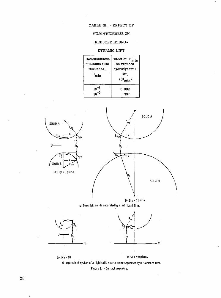
TABLE HI. - EFFECT OF

FILM THICKNESS ON

REDUCED HYDRO-

DYNAMIC LIFT

Dimensionlessminimum film

thickness,Hmin

ID"4

io-5

Effect of Hmin

on reducedhydrodynamic

lift,

^min*

0.992.997

UB 'Bx

rBx

(a-l)y = 0 plane.

(a-2)x = 0 plane,

(a) Two rigid solids separated by a lubricant film.

— x—i

"o

(b-1) y • 0 r (b-2) x »0 plane.

(b) Equivalent system of a rigid solid near a plane separated by a lubricant film.

Figure 1. - Contact geometry.

28

•S

.

.S

S,

29

2.0

•§

— O— Parabolic approximation— O— Full circular film----- Kapitza's analysis (ref. 1)

L(o)=7r /2I "

10 3015 20 25Radius ratio, a = Ry/Rx .

Figure 4. - Effect of radius ratio on reduced hydrodynamic lift.

35 4

Dimensionless central(minimum) film

thickness,Hl

.,- Iff

," 10'

Figure 5. - Pressure profiles along rolling direction for two film thicknesses.

30

Rollingdirection ""*

Captation/ boundary

Exit region

(a) Radius ratio, a, 1.00.

P

Rolling r

direction

Captation/ boundary

(b) Radius ratio, a. 36.54.

Figure 6. - Three-dimensional representations of pressure.distributionsas viewed from exit region, illustrating captation boundary.

31

.2Evt3

I

s

£a.

3CT.iZ

s? £

~ £•£-£•g. 8 8 8X .C .C £LLU I— I— I—

I

I

O I

I

_L I

- 5uo O)

"c^ jS

'wi1^ <U

P {

-o "g SiO o> (U

)̂ O.

s.ll• WO OJ

II

OM/°H 'spue peo| sssiuoisuauiip 0) ssaupjij) iu|L) IBJIUBD ssajuoisuauiip p oney

32

Figure 9. - Pressure profiles along rolling direction for dimensionless film thickness of 10"* with three radiusratios.

33

1. Report No. NASA TP-1287 2. Government Accession No.

AVRADCOM TR 78-18(PL)4. Title and Subtitle

EFFECT OF GEOMETRY ON HYDRODYNAMICFILM THICKNESS

7. Author(s)

David E. Brewe, Bernard J. Hamrock, andChristopher M. Taylor

9. Performing Organization Name and AddressNASA Lewis Research Center andAVRADCOM Research and Technology LaboratoriesCleveland, Ohio 44135

12. Sponsoring Agency Name and AddressNational Aeronautics and Space AdministrationWashington, D.C. 20546 and U.S. Army Aviation Research andDevelopment Command, St. Louis, Mo. 63166

3. Recipient's Catalog No.

5. Report Date

August 19786. Performing Organization Code

8. Performing Organization Report No.

E-934710. Work Unit No.

505-0411. Contract or Grant No.

13. Type of Report and Period Covered

Technical Paper14. Sponsoring Agency Code

15. Supplementary NotesDavid E. Brewe, AVRADCOM Research and Technology Laboratories; Bernard J. Hamrock,Lewis Research Center; Christopher M. Taylor, Lecturer in Mechanical Engineering,University of Leeds, Leeds, England, National Research Council - NASA Research Associate.Presentation at ASLE-ASME Joint Lubrication Conference, Minneapolis, Minn., Oct. 24-26, 1978

16. Abstract

The influence of geometry on the isothermal hydrodynamic film separating two rigid solidswas investigated. Pressure-viscosity effects were not considered. The minimum filmthickness is derived for fully flooded conjunctions by using the Reynolds boundary conditions.It was found that the minimum film thickness had the same speed, viscosity, and load de-pendence as Kapitza's classical solution. However, the incorporation of Reynolds boundaryconditions resulted in an additional geometry effect. Solutions using the parabolic film ap-proximation are compared with those using the exact expression for the film in the analysis.Contour plots are shown that indicate in detail the pressure developed between the solids.

17. Key Words (Suggested by Author(s))

Hydrodynamics; Film thickness; Bearings;Lubrication; Isothermal processes; Rollingcontact loads; Sliding; Reynolds equation;Leakage; Cavitation flow

18. Distribution Statement

Unclassified - unlimitedSTAR Category 37

19. Security Classif. (of this report)

Unclassified20. Security Classif. (of this page)

Unclassified

21. No. of Pages

34

22. Price"

A03

* For sale by the National Technical Information Service, Springfield. Virginia 22161NASA-Langley, 1978

National Aeronautics andSpace Administration

Washington, D.C.20546

Official Business

Penalty for Private Use, $300

THIRD-CLASS BULK RATE Postage and Fees PaidNational Aeronautics andSpace AdministrationNASA-451

NASA POSTMASTER' If Undeliverable (Section 158Postal Manual) Do Not Return