effects of asymmetric information on market timing in the
TRANSCRIPT

Munich Personal RePEc Archive
Effects of asymmetric information on
market timing in the mutual fund
industry
Tchamyou, Vanessa and Asongu, Simplice and Nwachukwu,
Jacinta
January 2018
Online at https://mpra.ub.uni-muenchen.de/87870/
MPRA Paper No. 87870, posted 12 Jul 2018 08:05 UTC

1
A G D I Working Paper
WP/18/007
Effects of asymmetric information on market timing in the mutual fund
industry
Forthcoming: International Journal of Managerial Finance
Vanessa S. Tchamyou
Faculty of Applied Economics, University of Antwerp, Antwerp Belgium
E-mails: [email protected] / [email protected]
Simplice A. Asongu
Development Finance Centre, Graduate School of Business,
University of Cape Town, Cape Town, South Africa. E-mails: [email protected] /
Jacinta C. Nwachukwu
School of Economics, Finance and Accounting, Faculty of Business and Law,
Coventry University Priory Street, Coventry, CV1 5FB, UK
Email: [email protected]

2
2018 African Governance and Development Institute WP/18/007
Research Department
Effects of asymmetric information on market timing in the mutual fund industry
Vanessa S. Tchamyou, Simplice A. Asongu & Jacinta C. Nwachukwu
January 2018
Abstract
The paper investigates the effects of information asymmetry (between the realised return and the
expected return) on market timing in the mutual fund industry. For the purpose, we use a panel of
1488 active open-end mutual funds for the period 2004-2013. We use fund-specific time-dynamic
betas. Information asymmetry is measured as the standard deviation of idiosyncratic risk. The
dataset is decomposed into five market fundamentals in order to emphasis the policy implications
of our findings with respect to (i) equity, (ii) fixed income, (iii) allocation, (iv) alternative and (v)
tax preferred mutual funds. The empirical evidence is based on endogeneity-robust Difference
and System Generalised Method of Moments. The following findings are established. First,
information asymmetry broadly follows the same trend as volatility, with a higher sensitivity to
market risk exposure. Second, fund managers tend to raise (cutback) their risk exposure in time of
high (low) market liquidity. Third, there is evidence of convergence in equity funds. We may
therefore infer that equity funds with lower market risk exposure are catching-up with their
counterparts with higher exposure to fluctuation in market conditions. The paper complements the
scarce literature on market timing in the mutual fund industry with time-dynamic betas,
information asymmetry and an endogeneity-robust empirical approach.
Key words: Information asymmetry; Mutual funds; Market timing; Market uncertainty
JEL Classification: G12; G14; G18
1.Introduction
The global financial crisis of 2008 had a huge impact on the fund industry due to the collapse of
many well established companies in the sector. This financial storm led to changes in investors’
habit, by inter alia: (i) reducing their market risk exposure and (ii) confronting them with liquidity
risk, systematic risk and other leverage effects (Fabozzi et al., 2010). Accordingly, investors failed
to anticipate the global financial meltdown substantially because they were unable to time the

3
United States
50%Europe
31%
Africa and Asia-
Pacific
12%
Other Americas
7%
Total worldwide mutual fund assets: $30.0 trillion
market properly1 (Tchamyou & Asongu, 2017). In essence, there are some dynamics like
modifications in the disclosure of the underlying asset or differences in investment scenarios, that
could not be captured by the timing ability of mutual fund managers (Bodson et al., 2013). It
logically follows that the market timing2 inability of fund managers prior to the underlying crisis
is most traceable to information asymmetry and market uncertainty. Though the fund industry
suffered from the 2008 financial crisis, active mutual funds3 are becoming increasingly popular.
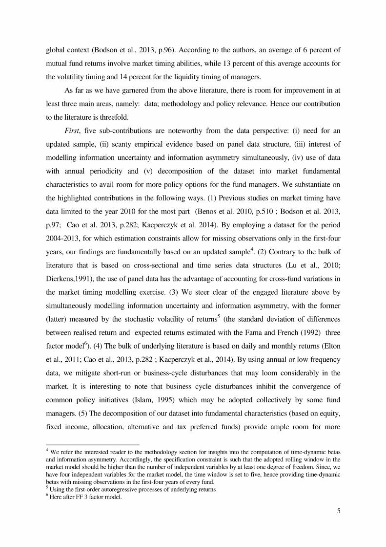
In addition, the United States in which the crisis originated still represents the largest mutual fund
market worldwide. As shown in Figure 1, there were $30 trillion worth of 7,707 open-end mutual
funds with a total net assets of $15,000 trillion by the end of the 2013, with the United States and
Europe representing 50 percent and 31 percent respectively (ICI, 2014).
Figure 1
Total worldwide mutual fund assets
Percentage of total net assets at the end of the year 2013
1 While scholars in financial engineering have been quick to recognize their inability to predict the recent financial crisis, according to Mitchell (2004, p. 76), future trends in social sciences are supposed to be predicted with almost mathematical precision. It is important to note that, even if fund managers were able to forecast the crisis, it would have happened anyway because of portfolio composition. In addition, they cannot exit the market and convert their asset into cash. 2 “The concept of “market timing” can potentially be generalized to include the systematic risk factors of the Carhart (1997) and Fama and French (1993) models as well. That is, if a manager could predict how the size (SMB), book-to-market (HML) and
momentum (MOM) factors would move, he could purchase stocks with high or low sensitivities to these factors in the exact same
way he would for the market”(Benos et al., 2010, p.509). 3 A Mutual fund is defined as a company which mobilizes financial resources from different investors for placement in securities like money-market funds, bonds, stocks, or the mix of these investments. It is usually classified into three principal types of investment companies: unit-investment trusts; open-end funds and closed-end funds (SEC, 2008). In this paper, active funds are relative to index and smart beta funds.

4
Source: 2014 Investment Company Fact Book
In the light of the above, researchers have had a renewed interest in the market timing
ability of active fund managers. We engage the available literature in two main strands: (i) pre-
and (ii) post-2008 financial crisis.
In the first strand, we tackle the literature prior to the 2008 financial crisis which also
highlights the theoretical underpinnings of the study. Since the fundamental research of Treynor
and Mazuy (1966), studies on the ability of fund managers to time the market have been widely
explored. Many authors including Treynor and Mazuy (1966); Kon (1983); Chang and Lewellen
(1984); Henriksson (1984); Lee and Rahman (1990); Busse (1999); Bollen and Busse, (2001)
and Jiang et al. (2007) worked on the ability of mutual fund managers to employ their predicting
capacity of future market returns to obtain abnormal returns. These authors investigated the timing
ability of mutual fund managers from different perspectives, notably in market returns, liquidity
and volatility. For example, with respect to volatility timing, Busse (1999) used daily mutual fund
returns to show that the ability of fund managers to time volatility is a substantial factor in
determining returns that could lead to higher risk-adjusted results.
The second stream of the literature embodies more recent studies on the timing ability of
mutual fund managers. Clare et al. (2016) employed two different methods — returns-based
method and holdings-based approach — to examine whether a multi-asset class is able to time the
market. Their results showed little evidence of the ability of fund managers to accurately time
multi-asset class. Kacperczyk et al. (2014) have suggested a new definition how to persistently
time the market with cognitive ability. They proposed a new measure of managers’ market timing
ability in periods of economic recession. Further, using monthly holding data to examine mutual
fund timing ability, Elton et al. (2011) found significantly positive results which show that
managers are able to time the market substantially. Frijns et al. (2013) proposed a new approach
based on a heterogeneous agent model; a switching rule between cash and stocks; to determine
the timing ability of mutual fund managers. Applying that rule to equity mutual funds, they found
that only 3.25 percent have positive timing ability whereas 41.5 percent have negative timing
skills. Liquidity timing has been assessed by Cao et al. (2013). They recommended that
investment managers could adapt their un-diversifiable risk based on the scale of aggregate
liquidity. To be sure, fund managers will tend to decrease their market exposure in periods of low
liquidity and vice-versa when liquidity increases. Their results indicated that mutual fund
managers reduced their exposure to market risk when global liquidity is low, sustaining the
position that mutual fund managers have an ability to time market liquidity. In addition,
perspectives of market volatility, market return and aggregate liquidity have been investigated in a
5
global context (Bodson et al., 2013, p.96). According to the authors, an average of 6 percent of
mutual fund returns involve market timing abilities, while 13 percent of this average accounts for
the volatility timing and 14 percent for the liquidity timing of managers.
As far as we have garnered from the above literature, there is room for improvement in at
least three main areas, namely: data; methodology and policy relevance. Hence our contribution
to the literature is threefold.
First, five sub-contributions are noteworthy from the data perspective: (i) need for an
updated sample, (ii) scanty empirical evidence based on panel data structure, (iii) interest of
modelling information uncertainty and information asymmetry simultaneously, (iv) use of data
with annual periodicity and (v) decomposition of the dataset into market fundamental
characteristics to avail room for more policy options for the fund managers. We substantiate on
the highlighted contributions in the following ways. (1) Previous studies on market timing have
data limited to the year 2010 for the most part (Benos et al. 2010, p.510 ; Bodson et al. 2013,
p.97; Cao et al. 2013, p.282; Kacperczyk et al. 2014). By employing a dataset for the period
2004-2013, for which estimation constraints allow for missing observations only in the first-four
years, our findings are fundamentally based on an updated sample4. (2) Contrary to the bulk of
literature that is based on cross-sectional and time series data structures (Lu et al., 2010;
Dierkens,1991), the use of panel data has the advantage of accounting for cross-fund variations in
the market timing modelling exercise. (3) We steer clear of the engaged literature above by
simultaneously modelling information uncertainty and information asymmetry, with the former
(latter) measured by the stochastic volatility of returns5 (the standard deviation of differences
between realised return and expected returns estimated with the Fama and French (1992) three
factor model6). (4) The bulk of underlying literature is based on daily and monthly returns (Elton
et al., 2011; Cao et al., 2013, p.282 ; Kacperczyk et al., 2014). By using annual or low frequency
data, we mitigate short-run or business-cycle disturbances that may loom considerably in the
market. It is interesting to note that business cycle disturbances inhibit the convergence of
common policy initiatives (Islam, 1995) which may be adopted collectively by some fund
managers. (5) The decomposition of our dataset into fundamental characteristics (based on equity,
fixed income, allocation, alternative and tax preferred funds) provide ample room for more
4 We refer the interested reader to the methodology section for insights into the computation of time-dynamic betas and information asymmetry. Accordingly, the specification constraint is such that the adopted rolling window in the market model should be higher than the number of independent variables by at least one degree of freedom. Since, we have four independent variables for the market model, the time window is set to five, hence providing time-dynamic betas with missing observations in the first-four years of every fund. 5 Using the first-order autoregressive processes of underlying returns 6 Here after FF 3 factor model.

6
targeted policy implications to managers concerned with only certain features of the fund
industry. This positioning is consistent with Elton et al. (2011) on the view that the available
literature is focused on equity funds for the most part (Kacperczyk et al., 2014; Bodson et al.,
2013; Benos et al.,2010).
Second, contributions on the methodological front are at least threefold. Accordingly, the
adopted empirical strategies: (i) accommodate the persistent nature of returns and corresponding
betas, (ii) account for cross-fund variations and endogeneity and (iii) compute time-dynamic
information uncertainty, information asymmetry and fund-specific betas. For brevity, these
empirical approaches which broadly steer clear of those adopted in the discussed literature are
substantially engaged in the methodology section.
Third, the policy relevance is at least threefold. (1) Essence of convergence or catch-up in
market exposure among funds. Accordingly, evidence of catch-up theoretically implies the
feasibility of common policy initiative among funds within a specific category or homogenous
panel. (2) Policy implications from fundamental characteristics are relevant because market
timing studies in the mutual fund industry have been based on equity funds for the most part.
There are growing calls for more complete studies that go beyond equity funds in the assessment
of mutual fund managers’ market timing abilities (Elton et al., 2011). (3) The distinction between
the effects of information asymmetry (hereafter IA) and uncertainty in market timing has crucial
policy relevance because these two concepts have been used interchangeably in prior expositions.
From a preliminary assessment based on correlation analysis, these two concepts do not appear to
display a high degree of substitution warranting concerns of over-parameterization.
In the light of the above, we complement existing literature by positioning the present line
of inquiry on the information asymmetry effects on market timing in the mutual fund industry.
Hence we devote space to (i) discussing the intuition of and theoretical underpinnings for the
study and (ii) clarifying the context of information asymmetry which is a complex and
multifaceted concept.
We estimate the effects of information asymmetry between fund managers and the market
in the mutual fund industry. Corresponding differences between the realised return (provided by
the market) and the expected return (by the fund manager) can be a source of information
mismatched which sometimes may mitigate the timing ability of mutual fund managers.
Asymmetry in information also refers to the lack of knowledge of the market by fund managers or
investors. Additionally, it shows that some managers have more knowledge about the firm value
because private information is at their disposal prior to the market (Dierkens, 1991, p.183). It also
refers to a situation where market players have different sets of information (Lu et al., 2010).

7
Consistent with our motivation and theoretical foundation, information asymmetry will
determine the choice of investment portfolios and strategies. Moreover, market exposure should
be an increasing function of market knowledge. Following Dai et al. (2013), Dierkens (1991) and
Ivashina (2009), we use the standard deviation of idiosyncratic risk of investors’ return as an
instrument of information asymmetry.
The rest of the paper proceeds as follows. Section 2 describes our dataset and discusses the
methodology. We tackle the empirical analysis, presentation of results and related policy
implications in Section 3. Section 4 concludes.
2. Data and Methodology
2.1. Data
Information on mutual fund data is sourced from Morningstar Direct for the period 2004-2013.
We have selected open-end mutual funds investing in domestic funds and we use the Global
Broad Category Group from the underlying source. The classification is made of 243 fixed
income funds, 882 equity funds, 156 allocation funds, 15 alternative funds and 186 tax-preferred
funds. We process the data to remove missing observations and ensure a strongly balanced panel
data structure made-up of 1488 mutual funds, with 10 annual observations.
2.2. Methodology
2.2.1 Estimation of volatility, beta and information asymmetry
There are different measures of information asymmetry in the existing literature, depending on the
study. Dierkens (1991) used four proxies to measure asymmetry of information between firm
managers and the market in the context of equity issues. Ivashina (2009) assessed the cost
resulting from irregularity in information between elements of a lending syndicate and the lead
bank. Consistent with the same definition, Dai et al. (2013) employed the standard deviation of
idiosyncratic risks of return in assessing how information unevenness and mutual fund ownership
influenced the earnings management of listed companies. A common denominator among these
studies is that asymmetric information is the difference between realised and expected returns.
Hence, in this study, information asymmetry is computed using the standard deviation of the
idiosyncratic risk of returns7. Idiosyncratic information asymmetry refers to the standard deviation
of the residuals of individual returns. Within the context of this study, while we use the Capital
7 The idiosyncratic risk of return is the same as abnormal returns. That is the difference between the realized return and the expected one.

8
Asset Pricing Model (CAPM) augmented with the FF three factor model (see Eq.2 below), a
stochastic modelling approach is employed to obtain the variable used as proxy for information
uncertainty or volatility.
Volatility of returns is computed as standard errors from first order auto-regressive
processes of the returns. Borrowing from Kangoye (2013) and Asongu et al. (2017), on the
computation of uncertainties or volatilities, auto-regressive models are used for low frequency
data. Hence, we apply this methodology since our dataset is made of annual open-end mutual
funds. The saved RMSE8 (Root-Mean_Square Error) of each return obtained from the first
autoregressive processes are used as uncertainty (or volatility). The computation process is
summarised in the following equation.
tititi TRR ,1,, (1)
Where tiR , is the return of fund i at time t ; 1, tiR the return of fund i at time 1t ; T
the time trend; the constant ; is the parameter of interest to be estimated and ti , the
error term.
We model mutual fund expected returns with the FF three-factor model to estimate fund-specific
systematic risk.
titiHMLtiSMBttiMKTitfti HMLSMBMKTRR ,,,,,,, (2)
Where fR is the risk free rate, MKT is the market excess return, SMB Small [market
capitalization] Minus Big [market capitalization] and HML High [book-to-market ratio]
Minus Low [book-to-market ratio]. The aforementioned three factors are taken from the
Kenneth French's website9.
A simple view of information asymmetry can then be modelled as follows:
tititi RRIA ,,, (3)
Where IA is Information Asymmetry; the standard deviation; tiR , the realised return of
fund i at time t ;
tiR , is the expected return computed using the FF three factor model.
We estimate time dynamic betas corresponding to each fund as a measure of market timing or
exposure. The advantage of having a time varying beta is that it captures more realistic changes in
8 The RMSE (Root-Mean-Square Error) can be used as the standard deviation of residuals or as a measure of uncertainty (Kitagawa & Okuda, 2013). 9 Kenneth French's website: http://mba.tuck.dartmouth.edu/pages/faculty/ken.french/data_library.html

9
market conditions since we have a different beta for each return and each year. Such is in line with
the wealth of literature cautioning that the beta of an asset may not be fixed over time (Ferson &
Schadt, 1996, p.428). The time-dynamic betas and RMSE for information asymmetry are
estimated from Equation 2 using the Rollreg Stata command. Given that the time-window must
be higher than the number of independent variables by at least one degree of freedom, we adopt a
five year moving-window such that we have only four missing observations for each fund.
To estimate the liquidity10 risk measure, we use the aggregate liquidity factors of the
updated series of Pástor and Stambaugh (2003). All factors are retrieved from Robert Stambaugh's
Website11 (See Bodson et al., 2013). Since we have annual mutual fund data and the liquidity
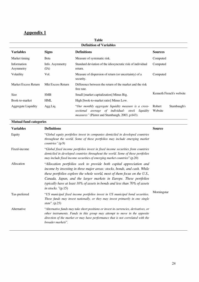
measures are in months, we compute annual averages using the monthly data. Appendix 1
presents the definition of variables.
Please insert Table 1 here.
Table 1 presents the summary statistics for mutual fund categories and variables in Panel A and
Panel B respectively. There is, at least, a twofold motivation for the disclosure. On the one hand,
we observe from the mean values that the variables are comparable. On the other, it shows from
the standard deviations that there is a substantial variability in the indicators. Therefore, some
statically significant relationships could be expected.
The correlation matrix presented in Table 2 below has two main objectives. It allows us to
mitigate errors arising from over-parameterization and multicollinearity between variables which
are simultaneously employed in the same model. In this regard ‘market excess return’ and
‘aggregate liquidity’ are not specified in the same model, since their correlation coefficient is
0.7498. The inference is that, approximately 74 percent of the aggregate liquidity risk can be
explained by market excess return. In other words a high scale of market liquidity can be linked
with a high measure of market return (Cao et al., 2013, p.285).
Consistent with the literature (Bodson et al., 2013), we have specified size and book-to-
market ratio in the same model for the estimation of the beta (market timing) despite their high
level of correlation.
Please insert Table 2 here.
10 “Aggregate liquidity” and “liquidity” are used interchangeably in the study. 11 Robert Stambaugh's Website: http://finance.wharton.upenn.edu/~stambaugh/

10
2.2.2 Model
The methodologies adopted in this paper are the difference and the system GMM (Generalized
Method of Moments). There are at least six main reasons for adopting this empirical strategy.
They are (i) cross-fund variation; (ii) persistence of betas; (iii) endogeneity; (iv) non-
contemporaneous specifications, (v) variation of variables and (vi) consistency with the data
structure.
First, contrary to time series specifications, the dynamic panel estimation technique
corrects for cross-fund variations in the determination of estimated coefficients. Hence, both time
series and cross-sectional variations are accounted for.
Second, return in the fund industry and corresponding betas have been documented to be
persistent (Carhart, 1997) and a fundamental condition for the employment of the GMM
estimation strategy is persistence in the dependent variable. Moreover, the auto-regressive
processes used in the computation of information uncertainty are based on the assumption of
persistence of the return variables.
Third, given that betas in the fund industry are endogeneous (Blocher, 2013) the adopted
estimation strategy controls for time invariant omitted variables (or unobserved heterogeneity)
and simultaneity bias through the use of instrumental variables.
Fourth, non-contemporaneous specifications make more economic sense than
contemporaneous regressions in the fund industry (Blocher, 2014). The instrumentation process in
the system GMM specification involves non-contemporary effects of the independent variables on
the outcome indicator.
Fifth, consistent with Bodson et al. (2013, p.98), the modelling of market timing is
tailored to capture changes in the variables. Hence, by taking changes (or deviations) into account,
the GMM specifications are consistent with modelling of the market timing ability of mutual
funds managers.
Sixth, the empirical strategy is consistent with data structure (N > T) => N = 1488 and T =
10. In essence, the GMM estimation technique is a good-fit for data structures in which N
(numbers of individuals/cross-sections) is large and T (time series/periods) is small (Arellano &
Bond, 1991).
The estimation technique is presented as follows, with Eq. (3) and Eq. (4) in level and first
difference respectively.
tititittittittittittti LiqVolIAMKT ,,,5,,4,,3,,21,,1,0, (4)

11
1,,11,,,51,,,4
1,,,31,,,22,1,,11,,
tititttitittitit
titittitittitittiti
LiqLiqVolVol
IAIAMKTMKT
,
(5)
where, ti , is the beta of fund i
at period t ; is a constant;
MKT , Market excess return ; IA,
Information Asymmetry; Vol , Volatility, Liq , Liquidity, i
is the country (or fund) -specific
effect, t is the time-specific constant and ti , the error term. To control for heteroscedasticity,
the two-step procedure has been preferred to the one-step procedure in the specification.
While the difference GMM approach is based on Eq. (5), the system GMM adds the level
equation to Eq. (5). Whereas the instrumentation procedure in the difference GMM entails the use
of lagged levels of the regressors as instruments, the process in the system GMM requires lagged
differences of the regressors as instruments in the level equation and lagged levels of the
regressors as instruments in the difference equation. This non-contemporanoeus dimension also
enables the exploitation of all orthogonality conditions between the lagged endogeneous variable
and the error term.
3.Empirical Analysis and Discussion of Results
3.1. Presentation of Results
Table 3 and Table 4 present the results of the regression analysis. Table 3 discloses the findings
of the difference GMM while Table 4 reveals the results for the system GMM. In the
specifications, not all independent variables are modelled together to avoid issues of over-
parameterization and multicollinearity already discussed above. The first two specifications
represent the baseline model while the remaining models are for each of our five categories of
mutual funds: equity; fixed income; allocation; alternatives and tax-preferred funds. This enables
us to assess if the reaction of a mutual fund manager in timing the market is sensitive to fund type.
All specifications are robust to heteroscedasticity because we have adopted a two-step procedure.
Time fixed effects are also taken into account in all specifications.
Most of the variables have the expected signs. (1) Information asymmetry is significantly negative
in the baseline model (Table 4), equity funds (Table 4), fixed income funds (Table 3 and Table 4)
and allocation funds (Table 4). Unexpected positive signs are found in tax-preferred funds. (2)
Volatility is significantly negative except for the allocation funds. (3) Aggregate liquidity is
expectedly positive and statistically significant for all our fund types, with the exception of

12
allocation funds. (4) Market excess return in the baseline model (first specification) is not
significant. But in the regression for fixed income and alternative funds, we find positive
significant results contrary to the significantly negative association estimated for the equity mutual
fund.
The validity of the models based on the information criteria is appealing for the most part.
Accordingly, the Wald Chi-square for the overall validity of models is overwhelmingly significant
at a 1 percent level. Additionally, following a rule of thumb, the number of instruments is
generally lower than the number of cross-sections. This implies that most of our results do not
really suffer from instrument proliferation or over-identification (difference between instruments
and endogeneous explanatory variables).
Please insert Table 3 and Table 4 here.
3.2. Further Discussion of Results and Policy Implications
In this sub-section, we discuss the results with related policies in three main areas. First, we report
the global relevance of our baseline specifications in Table 3 and Table 4 for difference and
system GMM estimations respectively. Second, we further explain the meaning and implication
of our findings by fund categories and finally, we emphasise the consequences for convergence.
3.2.1. Global results
Policy implications are deduced based on the results in Table 3 and Table 4. More specifically, we
focus on those recommendations which could be adapted by managers to suit the investment
profile of each fund category.
Results in the first two columns of the baseline model in Table 3 and Table 4 show that most of
the variables have the expected signs. First, the significant negative outcomes in Table 4 are
predictable given that asymmetry in information in this study is measured as the difference
between realised and expected returns12. Thus, its expected sign should intuitively be the same as
that of volatility. Second, the negative sensitivity of the volatility timing ability of fund manager is
consistent with the empirical underpinnings on the association between high levels of volatility
12 It is important to note that, if the information asymmetry were between managers and investors, we would have expected opposite or positive signs because increasing positive information asymmetry between them is more likely to increase the earnings management of fund managers. Conversely, higher information asymmetry between fund managers and the market within the context of this study implies fund managers are likely to predict future market returns, hence a potentially decreasing earnings management. This intuition is consistent with Dai et al. (2013, p.197), who have shown that when information asymmetry between investors and fund managers is low, earnings management deteriorates.

13
and systematic risk (Bodson et al., 2013; Cao et al., 2013; Busse, 1999). Third, liquidity timing is
positive and significant. This means that managers of funds accurately predict high (low) liquidity
market and therefore increase (or decrease) their exposure to the market (Cao et al. 2013). Fourth,
generally speaking, the findings in Column 1 of Table 3 and Table 4 indicate that fund managers
do not have substantial return timing ability. This is essentially because the effect of excess
market return is not consistently significant. Accordingly, excess market return should increase
market exposure. This conclusion is consistent with Bodson et al. (2013).
So far, we have exclusively reported the signs of the independent variables of interest. But
for more subtlety in the policy implications it is also worthwhile to comparatively discuss the
magnitude of estimated coefficients which can also be understood as the ‘degree of
responsiveness of fund managers’ to market exposure. Broadly speaking, for both Table 3 and
Table 4, two practical implications are apparent: First, the negative sensitivity of volatility is
higher than that of information asymmetry13. This finding is in line with those of (Busse, 1999)
who remarked that negative volatility may lead to risk adjusted competitiveness. As far as we are
aware, there is no comparable literature on information asymmetry in mutual fund industry with
which to compare the findings. Additionally, in the context of this work, volatility and
information asymmetry are following the same trend. Hence, they may have the same economic
interpretation. Second the positive effect of aggregate liquidity is higher compared with the
negative impact of volatility and information asymmetry14. The higher positive response of
liquidity is an indication that managers may have capabilities to forecast performance of mutual
funds accurately. Moreover, after verifying the effect of volatility, liquidity is an important factor
in the market timing strategy of fund managers (Cao et al., 2013).
3.2.2. Results per fund category
For the specifications based on different fund categories, results are generally in accordance with
the global findings, but with some notable exceptions. In Table 3, information asymmetry has
significant positive effect on the tax preferred funds and negative impact on the fixed income
funds. In Table 4, results are almost the same as in Table 3, but with significant negative
13 This comparison does not take variable relativity into account. 14 Whereas the effect of information asymmetry is not significantly negative in Table 3, the System GMM results take precedence over the Difference estimators because the former estimation technique has been documented to be more efficient (Bond et al., 2001). “We also demonstrate that more plausible results can be achieved using a system GMM
estimator suggested by Arellano and Bover (1995) and Blundell and Bond (1998). The system estimator exploits an
assumption about the initial conditions to obtain moment conditions that remain informative even for persistent series,
and it has been shown to perform well in simulations. The necessary restrictions on the initial conditions are
potentially consistent with standard growth frameworks, and appear to be both valid and highly informative in our
empirical application. Hence we recommend this system GMM estimator for consideration in subsequent empirical
growth research”. (pp. 3-4)

14
outcomes for the baseline models and equity funds. No significant results for the alternative
mutual funds.
Predictably, volatility has a negative sign in both the baseline model and for each of our
selected mutual funds in Table 3 and Table 4. The inference is that fund would tend to reduce
their risk exposure in periods when an increase in market volatility is predictable. No significant
results are found for tax preferred mutual funds in Table 3 and Table 4; and fixed income funds in
Table 4. However, we found positive and significant signs for allocation funds in both tables,
meaning that the manager will be substantially exposed to risk. We found the same trend of
results for market excess return in the two tables: significantly negative results for equity funds
and no substantial outcome for the other fund types. As seen above, this may reflect that fact that
managers of mutual funds do not seem to have the ability to forecast their returns with reasonable
accuracy. However, significant positive results for fixed income and alternative funds were found
in both tables.
On the liquidity timing aspect, we found significant positive results for equity and fixed
income funds in both tables. These results are consistent with baseline specifications and in
accordance with the empirical underpinnings. Allocation funds are reacting differently from what
we have expected in terms of liquidity timing. In fact, we find negative significant signs. There is
no evidence of liquidity timing in allocation and tax-preferred funds in both tables.
3.2.3. Convergence and catch-up in market exposure
In this section, we briefly summarise the significance and economic relevance of the estimated
coefficients on our lagged endogenous variable. Consistent with the underlying literature (Islam,
2003), alpha convergence is a reduction of differences in market exposure from a cross-sectional
perspective whereas beta convergence is diminishing cross-fund dispersions from a panel stand
point. Accordingly, the term catch-up has been employed in mainstream literature to describe
beta convergence because of initial endowments and multiple equilibria issues associated with its
modelling. Hence, we shall employ the term ‘catch-up’ for consistency. Moreover, it is interesting
to note that ‘beta catch-up’ by definition is not ‘fund beta catch-up’. It is just a double coincidence
that the dependent variable employed in this study is termed in ‘financial jargon’ the same as the
concept of catch-up in ‘economic jargon’. Hence, for simplicity we employ ‘catch-up’
interchangeably for ‘beta catch-up’ and ‘fund beta catch-up’.
The version of beta catch-up employed is the conditional catch-up, as opposed to the
absolute catch-up version which is not contingent on some conditioning information set or

15
explaining variables. The conditional version is more relevant to this study because catch-up in
fund market exposure is contingent on the underlying determinants, notably: information
asymmetry, volatility, market excess return and liquidity. Hence, for conditional catch-up to occur
there should theoretically be cross-fund differences in the determinants of fund market exposure.
In other words, difference should exist among funds in the underlying explaining variables.
Catch-up in fund market exposure implies that funds with lower exposure are catching-up
with their counterparts with higher exposure. In other words, the marginal productivity effects of
some (or all) of the underlying determinants are higher for funds with initially lower levels of
exposure. This interpretation is consistent with the narrative on the higher marginal capital
productivity of per capita income in the mainstream convergence literature (Barro & Sala-i-
Martin, 1992)15. From a contextual perspective, the catch-up process means that the Left Hand
Side of Eq. (5) is decreasing over time because past differences have a less proportional effect on
future differences.
Evidence of catch-up is established from our findings if (i) the estimated coefficient on the
lagged endogenous variable is statistically significant at the five percent level and (ii) its
corresponding absolute value is between 0 and 1. From our findings, this information criterion
holds only for baseline and equity fund results.
Four main implications can be established. First, from a broad perspective, funds with lower
market exposure are catching-up their counterparts with higher market exposure. Second, when
the dataset is disaggregated into fund-specific categories this catch-up pattern is only apparent for
equity funds. This evidence is supported by the fact that, of the 1488 sampled funds in the
industry there are 882 equity funds. It should be noted that the absence of convergence in other
funds does not imply divergence because an information criterion for such a conclusion (or
equation) to the best of our knowledge has not yet been properly worked-out in the literature.
Third, a practical implication for catch-up in market exposure among funds managers in the
industry is the feasibility of common policy initiatives that can be applied without distinction of
funds’ localities and/or nationalities from which underlying fund managers operate. Such
feasibility in policy harmonization is particularly relevant in mitigating or averting far-reaching
negative tendencies in fund management that may have very negative implications like the global
financial crisis. Fourth, catch-up in the fund industry has financial relevance because
theoretically, in the presence of full catch-up, the possibility of supernormal profits among fund
15 Developing countries will grow at faster rate than advanced nations because of higher marginal productivity of capital. Hence, the development catch-up process.

16
managers disappear, such that fund managers with the same levels of information asymmetry and
volatility forecast have the same levels of returns from the common market.
4. Conclusion
In this paper we have investigated the effects of information asymmetry on market timing in the
mutual fund industry. The empirical analysis is based on different fund categories: equity funds;
fixed income funds; allocation funds; alternative funds and tax preferred funds. The following
findings have been established. First, information asymmetry broadly follows the same trend as
volatility, meaning that while fund managers reduce their risk exposure to the underlying factors,
their responsiveness to volatility is higher relative to information asymmetry. Second, with respect
to liquidity, fund managers tend to raise (cutback) their risk exposure in time of high (low) market
liquidity. Third, we also find evidence of convergence in equity funds, implying that equity funds
with lower market exposure are catching-up their counterparts with higher market exposure.
Understanding the timeline for the catch-up process could provide the basis for common
policies among fund managers in the industry. While we have resisted the temptation of involving
this dimension because it is out of the scope of the present study, it remains an interesting future
line of inquiry. Other further research directions may comprise, inter alia (i) assessing the
investigated factors throughout the conditional distributions of market exposure to address the
potential downsides of blanket policies based on estimated strategies that are focused on mean
values of market exposure and (ii) examining thresholds for which the sensitivity of fund
managers’ market timing abilities are based.

17
Table 1
Summary statistics
This table presents the summary statistics of fund categories (Panel A) and variables used in our analysis (Panel B).
Panel A: Mutual fund categories
Variables Mean Std. Dev. Min Max Obs.
Equity 0.5927419 0.4913402 0 1 14880
Fixed Income 0.1633065 0.3696575 0 1 14880
Allocation 0.1048387 0.3063558 0 1 14880
Alternative 0.0100806 0.0998984 0 1 14880
Tax Preferred 0.125 0.33073 0 1 14880
Panel B: Variables
Beta -0.018 0.932 -4.502 4.571 8928
Info. Asymmetry 19.467 15.245 0.000 93.425 8928
Volatility 25.980 12.115 0.691 64.902 7440
Mkt Excess Return 8.578 19.038 -38.39 35.15 14880
SMB 3.003 7.485 -7.01 17.74 14880
HML 2.411 12.342 -21.55 23.66 14880
Aggregate Liquidity -0.025 0.028 -0.098 0.010 14880 SMB: Size. HML: Book to market. Std. Dev.: Standard Deviation. Min.: Minimum. Max. : Maximum. Obs.: Observations.
Table 2
Correlation matrix
This table presents the correlation matrix of variables used in our analysis
Info.
Asymmetry
Volatility Mkt Excess
Return
SMB HML Aggregate
Liquidity
Beta
1.0000 0.1868 -0.0125 -0.0413 -0.0307 0.0137 0.0186 Info. Asymmetry
1.0000 -0.0418 -0.0308 -0.0090 0.0337 0.0050 Volatility
1.0000 0.5516 0.5184 0.7498 0.0231 Mkt Excess Return
1.0000 0.7186 0.0298 -0.0201 SMB
1.0000 0.2964 0.0123 HML
1.0000 0.0512 Aggregate Liquidity
1.0000 Beta
SMB: Size. HML: Book to market.

18
P-values are in brackets. *, **, ***: significance levels of 10%, 5% and 1% respectively. Numbers of Obs.: Numbers of observations. Num. of Cross-sec.: Numbers of Cross-sections. Numbers of Ins.: Numbers of Instruments.
Table 3
Regression Analysis
This table presents the regression analysis for the Difference GMM
Difference GMM (xtabond) (Dependent variable: Beta)
Baseline
Equity
Fixed Income
Allocation
Alternative
Tax Preferred
Constant 0.146** 0.176** 0.233* 0.264*** -0.171 0.139 -0.301 -0.335* 0.250 0.539* -0.264 -0.188 (0.037) (0.014) (0.015) (0.005) (0.170) (0.298) (0.165) (0.064) (0.174) (0.086) (0.168) (0.452) Beta(-1) -0.535*** -0.557*** -0.279** -0.337*** -1.062*** -1.264*** 0.176 0.154 -0.166 -0.214 -3.154*** -3.173***
(0.000) (0.000) (0.007) (0.002) (0.000) (0.000) (0.310) (0.336) (0.822) (0.695) (0.000) (0.000) Info. Asymmetry -0.000 -0.001 -0.000 -0.000 -0.005* -0.007*** -0.002 -0.003 -0.001 -0.004 0.016*** 0.015***
(0.539) (0.155) (0.950) (0.776) (0.015) (0.001) (0229) (0.198) (0.884) (0.635) (0.000) (0.000) Volatility -0.005* -0.005* -0.007** -0.006** -0.004 -0.009* 0.016*** 0.017** -0.039** -0.033** -0.000 -0.003 (0.056) (0.053) (0.042) (0.038) (0.278) (0.036) (0.009) (0.011) (0.022) (0.033) (0.901) (0.562) Mkt Excess Return 0.000 --- -0.003** --- 0.012*** --- 0.001 --- 0.019* --- -0.002 --- (0.396) (0.032) (0.000) (0.526) (0.076) (0.210) Aggregate Liquidity --- 3.111*** --- 7.894*** --- 2.872 --- -6.706*** --- -3.558 --- 2.325 (0.000) (0.000) (0.109) (0.005) (0.329) (0.307) Information criteria Numbers of Obs. 5952 5952 3528 3528 972 972 624 624 60 60 744 744 Num. of Cross-sec. 1488 1488 882 882 243 243 156 156 15 15 186 186 Numbers of Ins. 14 14 14 14 14 14 14 14 14 14 14 14 Wald Chi2 39.20*** 49.63*** 12.38** 54.65*** 60.71*** 37.71*** 9.01* 11.51** 7.31 13.44*** 222.16*** 224.71***
(0.000) (0.000) (0.014) (0.000) (0.000) (0.000) (0.060) (0.021) (0.120) (0.009) (0.000) (0.000)

19
P-values are in brackets. *, **, ***: significance levels of 10%, 5% and 1% respectively. Numbers of Obs.: Numbers of observations. Num. of Cross-sec.: Numbers of Cross-sections. Numbers of Ins.: Numbers of Instruments.
Table 4
Regression Analysis
This table presents the regression analysis for the System GMM
System GMM (xtdpdsys) (Dependent variable: Beta)
Baseline
Equity
Fixed Income
Allocation
Alternative
Tax Preferred
Constant 0.307*** 0.264*** 0.490*** 0.384*** -0.182 0.000 -0.251 -0.313* 0.160 0.468 -0.200 -0.359 (0.000) (0.000) (0.000) (0.000) (0.230) (0.997) (0.194) (0.061) (0.630) (0.324) (0.302) (0.103) Beta (-1) -0.683*** -0.681*** -0.482*** -0.530*** -1.482*** -1.365*** 0.073 0.040 -0.278 -0.382 -1.207*** -1.226***
(0.000) (0.000) (0.000) (0.000) (0.000) (0.000) (0.668) (0.817) (0.626) (0.446) (0.000) (0.000) Info. Asymmetry -0.002** -0.002** -0.003** -0.002** -0.005** -0.004* -0.004** -0.007** -0.001 -0.003 0.009*** 0.011***
(0.016) (0.014) (0.016) (0.027) (0.035) (0.081) (0.037) (0.045) (0.807) (0.768) (0.000) (0.000) Volatility -0.007*** -0.008*** -0.010*** -0.011*** 0.000 -0.004 0.017*** 0.019*** -0.035** -0.037 0.006 0.007 (0.003) (0.000) (0.002) (0.000) (0.983) (0.382) (0.004) (0.001) (0.010) (0.115) (0.444) (0.369) Mkt Excess Return -0.000 --- -0.006*** --- 0.009*** --- 0.001 --- 0.019* --- 0.000 --- (0.558) (0.001) (0.000) (0.575) (0.081) (0.738) Aggregate Liquidity --- 4.631*** --- 8.660*** --- 4.518** --- -7.961*** --- -7.192 --- -3.399 (0.000) (0.000) (0.023) (0.000) (0.423) (0.139) Information criteria Numbers of Obs. 7440 7440 4410 4410 1215 1215 780 780 75 75 930 930 Num. of Cross-sec. 1488 1488 882 882 243 243 156 156 15 15 186 186 Numbers of Ins. 18 18 18 18 18 18 18 18 18 18 18 18 Wald Chi² 87.68*** 110.61*** 41.94*** 103.6*** 54.08*** 50.97*** 12.60** 19.66*** 22.08*** 16.44*** 51.29*** 65.24***
(0.000) (0.000) (0.000) (0.000) (0.000) (0.000) (0.013) (0.000) (0.000) (0.002) (0.000) (0.000)
20
References
Arellano, M., & Bond, S., 1991. Some tests of specification for panel data: Monte Carlo
evidence and an application to employment equations. Review of Economic Studies, 58,
pp. 277–297.
Arellano, M., & Bover, O., 1995. Another Look at the Instrumental Variable Estimation of
Error Component Model. Journal of Econometrics, 68, pp. 29-52.
Asongu, S. A., Koomson, I.,& Tchamyou, V. S., 2017. Financial Globalisation
Uncertainty/Instability Is Good for Financial Development. Research in International
Business and Finance, 41 (October), pp. 280-291.
Barro, R. J., & Sala-i-Martin, X., 1992. Convergence. Journal of Political Economy, 100(2),
pp. 223-251.
Benos, E., Jochec, M. & Nyekel, V., 2010. Can mutual funds time risk factors? The Quarterly
Review of Economics and Finance, 50(4), pp.509–514.
Bodson, L., Cavenaile, L. & Sougné, D., 2013. A global approach to mutual funds market
timing ability. Journal of Empirical Finance, 20, pp.96–101.
Bollen, N.P.B. & Busse, J.A., 2001. On the Timing Ability of Mutual Fund Managers.
Journal of Finance, 56(3), pp.1075–1094.
Bond, S., Hoeffler, A., & Tample, J., 2001. GMM Estimation of Empirical Growth Models.
University of Oxford, Oxford.
Blocher, J., 2014. Network Externalities in Mutual Funds. PhD Thesis, p 4.
Blocher, J., 2013. Peer Effects in mutual funds. PhD Thesis.
Busse, J.A., 1999. Volatility Timing in Mutual Funds: Evidence from Daily Returns. Review
of Financial Studies, 12(5), pp.1009–1041.
Cao, C., Simin, T.T. & Wang, Y., 2013. Do mutual fund managers time market liquidity?
Journal of Financial Markets, 16(2), pp.279–307.

21
Carhart, M.M., 1997. On Persistence in Mutual Fund Perfomance. Journal of Finance, 52(1),
pp.57–82.
Chang, E., & Lewellen, W., 1984. Impact of size and flows on performance for funds of
hedge funds. Journal of Business, 57 (1), pp.57–72.
Clare, A., Ferguson, N., Sherman, M., & Thomas, S., 2016. Multi-asset class mutual funds:
Can they time the market? Evidence from the US, UK and Canada. Research in
International Business and Finance, 36 (2016) 212–221.
Dai, Y., Kong, D. & Wang, L., 2013. Information asymmetry, mutual funds and earnings
management: Evidence from China. China Journal of Accounting Research, 6(3),
pp.187–209.
Dierkens, N., 1991. Information Asymmetry and Equity Issues. Journal of Financial and
Quantitative Analysis, 26(2), pp.181–199.
Elton, E.J., Gruber, M.J. & Blake, C.R., 2011. An examination of mutual fund timing ability
using monthly holdings data. Review of Finance, 16(3), pp.619–645.
Fabozzi, F.J., Focardi, S.M. & Jonas, C., 2010. Investment Management after the Global
Financial Crisis, Research Foundation of CFA Institute.
Fama, E., & French, K. 1993. Common risk factors in the returns on stocks and bonds.
Journal of Financial Economics, 33, pp.3–56.
Fama, E., & French, K., 1992. The cross-section of expected stock returns. Journal of
Finance, 47 (2), pp.427–465.
Ferson, W.E., & Schadt, R.W., 1996. Measuring fund strategy and performance in changing
economic conditions. Journal of Finance, 51, pp.425–461.
Frijns, B., Gilbert, A. & Zwinkels, R.C.J., 2013. Market timing ability and mutual funds: a
heterogeneous agent approach. Quantitative Finance, 13(10), pp.1613–1620.
Henriksson, R.D., 1984. Market Timing and Mutual funds perfomance: An Empirical
Investigation. Journal of Business, 57(1, Part 1), pp.73–96.
22
ICI, 2014. Recent Mutual Fund Trends, In A Review of Trends and Activities in the U.S.
Investment Company Industry, (54th Edition 2014) Investment Company Fact Book,:
Chapter 2: pp. 25-52 ; Investment Company Institute.
Islam, N., 2003. What have we learnt from the convergence debate?. Journal of Economic
Surveys, 17(3), pp. 309-362.
Islam, N., 1995. Growth Empirics: A Panel Data Approach. The Quarterly Journal of
Economics, 110(4), pp.1127-1170.
Ivashina, V., 2009. Asymmetric information effects on loan spreads. Journal of Financial
Economics, 92(2), pp.300–319.
Jiang, G., Yao, T., & Yu, T., 2007. Do mutual funds time the market? Evidence from
portfolio holdings. Journal Financial Economics, 86 (3), pp.724–758.
Kacperczyk, M., Nieuwerburgh, S.V.A.N. & Veldkamp, L., 2014. Time-Varying Fund
Manager Skill. Journal of Finance, 69(4).
Kangoye, T., 2013. Does aid unpredictability weaken governance? Evidence from developing
countries. Developing Economies, 51(2), pp.121–144.
Kitagawa, N. & Okuda, S., 2013. Management Forecasts , Idiosyncratic Risk , and
Information Envionment. Working Paper, 38, pp.1–44.
Kon, S.J., 1983. The market timing performance of mutual fund managers. Journal of
Business, 56(3), pp.323–347.
Lee, C. & Rahman, S., 1990. Market timing, selectivity, and mutual fund performance: an
empirical investigation. Journal of Business, 63 (2), 261–278.
Lu, C.-W., Chen, T.-K. & Liao, H.-H., 2010. Information uncertainty, information asymmetry
and corporate bond yield spreads. Journal of Banking & Finance, 34(9), pp.2265–2279.
Mitchell, T., (2004). The Middle East in the Past and Future of Social Science. David Szanton
(ed.), The Politics of Knowledge: Area Studies and the Disciplines (University of
California Press; Berkeley), pp. 74-118.

23
Morningstar, 2014. The Morningstar Global Category Classifications. Morningstar
Methodology Paper Effective as of April 30, 2014.
Pástor, L. & Stambaugh, R.F., 2003. Liquidity Risk and Expected Stock Returns. The Journal
of Political Economy, 111(3), pp.642–685.
SEC, 2008. Mutual Funds - A Guide for investors. U.S. Securities and Exchange Community.
Tchamyou, V. S. & Asongu, S. A., 2017. Conditional Market Timing in the Mutual Fund
Industry. Research in International Business and Finance. 42 (December), pp. 1355-
1366.
Treynor, J., & Mazuy, K., 1966. Can mutual funds outguess the market? Harvard Business
Review, 44 (4), pp.131–136.
24
Appendix 1
Table
Definition of Variables
Variables Signs Definitions Sources
Market timing Beta Measure of systematic risk. Computed
Information
Asymmetry
Info. Asymmetry
(IA)
Standard deviation of the idiosyncratic risk of individual
return.
Computed
Volatility Vol. Measure of dispersion of return (or uncertainty) of a
security.
Computed
Market Excess Return Mkt Excess Return Difference between the return of the market and the risk
free rate.
Kenneth French's website
Size SMB Small [market capitalization] Minus Big.
Book-to-market HML High [book-to-market ratio] Minus Low.
Aggregate Liquidity Agg.Liq. “Our monthly aggregate liquidity measure is a cross-
sectional average of individual- stock liquidity
measures” (Pástor and Stambaugh, 2003, p.643).
Robert Stambaugh's
Website
Mutual fund categories
Variables Definitions Source
Equity “Global equity portfolios invest in companies domiciled in developed countries
throughout the world. Some of these portfolios may include emerging market
countries”.(p.9)
Morningstar
Fixed-income “Global fixed income portfolios invest in fixed income securities from countries
domiciled in developed countries throughout the world. Some of these portfolios
may include fixed income securities of emerging market countries”.(p.20)
Allocation “Allocation portfolios seek to provide both capital appreciation and
income by investing in three major areas: stocks, bonds, and cash. While
these portfolios explore the whole world, most of them focus on the U.S.,
Canada, Japan, and the larger markets in Europe. These portfolios
typically have at least 10% of assets in bonds and less than 70% of assets
in stocks.”(p.15)
Tax-preferred “US municipal fixed income portfolios invest in US municipal bond securities.
These funds may invest nationally, or they may invest primarily in one single
state”. (p.25)
Alternative “Alternative funds may take short positions or invest in currencies, derivatives, or
other instruments. Funds in this group may attempt to move in the opposite
direction of the market or may have performance that is not correlated with the
broader markets”.