EECS 442 – Computer vision

Object Recognition

• Intro

• Recognition of 3D objects

• Recognition of object categories:

• Bag of world models

• Part based models

• 3D object categorization

Computer Vision: Algorithms and Applications. R. Szeliski

Pages 696-709

Categorical vs Single Instance

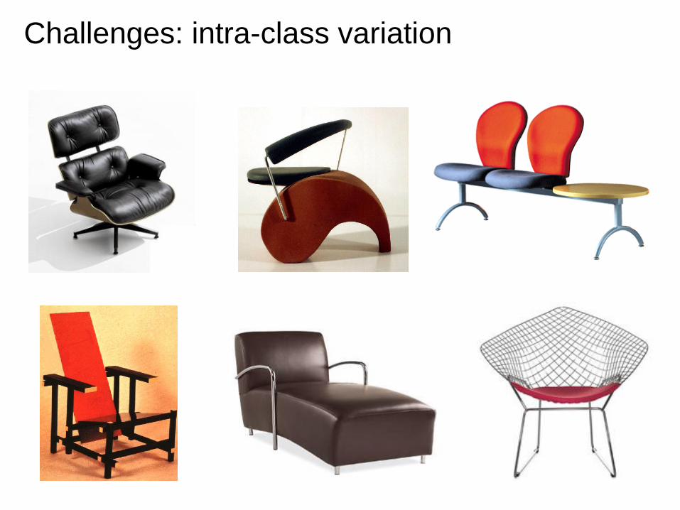
Challenges: intra-class variation

Challenges:

Variability due to:

• View point

• Illumination

• Occlusions

• Etc..

Basic properties

• Representation

– How to represent an object category; which classification scheme?

• Learning

– How to learn the classifier, given training data

• Recognition

– How the classifier is to be used on novel data

Part 1: Bag-of-words models

This segment is based on the tutorial “Recognizing and Learning

Object Categories: Year 2007”, by Prof A. Torralba, R. Fergus and F. Li

Related works

• Early “bag of words” models: mostly texture recognition – Cula & Dana, 2001; Leung & Malik 2001; Mori, Belongie & Malik,

2001; Schmid 2001; Varma & Zisserman, 2002, 2003; Lazebnik, Schmid & Ponce, 2003;

• Hierarchical Bayesian models for documents (pLSA, LDA, etc.) – Hoffman 1999; Blei, Ng & Jordan, 2004; Teh, Jordan, Beal &

Blei, 2004

• Object categorization – Csurka, Bray, Dance & Fan, 2004; Sivic, Russell, Efros,

Freeman & Zisserman, 2005; Sudderth, Torralba, Freeman & Willsky, 2005;

• Natural scene categorization – Vogel & Schiele, 2004; Fei-Fei & Perona, 2005; Bosch,

Zisserman & Munoz, 2006

Object Bag of ‘words’

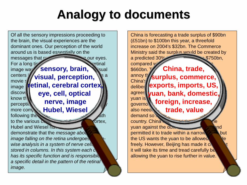
Analogy to documents

Of all the sensory impressions proceeding to

the brain, the visual experiences are the

dominant ones. Our perception of the world

around us is based essentially on the

messages that reach the brain from our eyes.

For a long time it was thought that the retinal

image was transmitted point by point to visual

centers in the brain; the cerebral cortex was a

movie screen, so to speak, upon which the

image in the eye was projected. Through the

discoveries of Hubel and Wiesel we now

know that behind the origin of the visual

perception in the brain there is a considerably

more complicated course of events. By

following the visual impulses along their path

to the various cell layers of the optical cortex,

Hubel and Wiesel have been able to

demonstrate that the message about the

image falling on the retina undergoes a step-

wise analysis in a system of nerve cells

stored in columns. In this system each cell

has its specific function and is responsible for

a specific detail in the pattern of the retinal

image.

sensory, brain,

visual, perception,

retinal, cerebral cortex,

eye, cell, optical

nerve, image

Hubel, Wiesel

China is forecasting a trade surplus of $90bn

(£51bn) to $100bn this year, a threefold

increase on 2004's $32bn. The Commerce

Ministry said the surplus would be created by

a predicted 30% jump in exports to $750bn,

compared with a 18% rise in imports to

$660bn. The figures are likely to further

annoy the US, which has long argued that

China's exports are unfairly helped by a

deliberately undervalued yuan. Beijing

agrees the surplus is too high, but says the

yuan is only one factor. Bank of China

governor Zhou Xiaochuan said the country

also needed to do more to boost domestic

demand so more goods stayed within the

country. China increased the value of the

yuan against the dollar by 2.1% in July and

permitted it to trade within a narrow band, but

the US wants the yuan to be allowed to trade

freely. However, Beijing has made it clear that

it will take its time and tread carefully before

allowing the yuan to rise further in value.

China, trade,

surplus, commerce,

exports, imports, US,

yuan, bank, domestic,

foreign, increase,

trade, value

– Independent features

definition of “BoW”

face bike violin

definition of “BoW”

– Independent features

– histogram representation

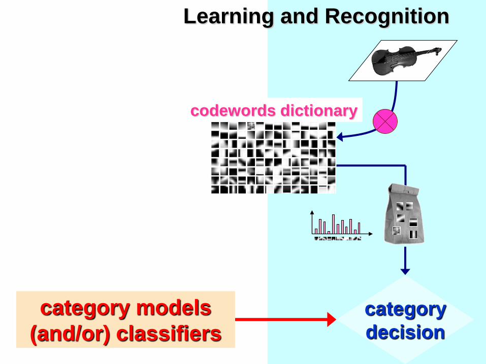
codewords dictionary

category

decision

Representation

feature detection

& representation

codewords dictionary

image representation

category models

(and/or) classifiers

recognition le

arn

ing

1.Feature detection and representation

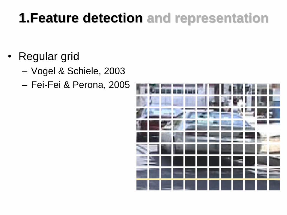
1.Feature detection and representation

• Regular grid

– Vogel & Schiele, 2003

– Fei-Fei & Perona, 2005

1.Feature detection and representation

• Regular grid

– Vogel & Schiele, 2003

– Fei-Fei & Perona, 2005

• Interest point detector

– Csurka, et al. 2004

– Fei-Fei & Perona, 2005

– Sivic, et al. 2005

1.Feature detection and representation

• Regular grid – Vogel & Schiele, 2003

– Fei-Fei & Perona, 2005

• Interest point detector – Csurka, Bray, Dance & Fan, 2004

– Fei-Fei & Perona, 2005

– Sivic, Russell, Efros, Freeman & Zisserman, 2005

• Other methods – Random sampling (Vidal-Naquet & Ullman, 2002)

– Segmentation based patches (Barnard, Duygulu, Forsyth, de Freitas, Blei, Jordan, 2003)

1.Feature detection and representation

Normalize

patch

Detect patches

[Mikojaczyk and Schmid ’02]

[Mata, Chum, Urban & Pajdla, ’02]

[Sivic & Zisserman, ’03]

Compute

SIFT

descriptor

[Lowe’99]

Slide credit: Josef Sivic

…

1.Feature detection and representation

2. Codewords dictionary formation

…

Example: color feature

r

b

g

Example: color feature

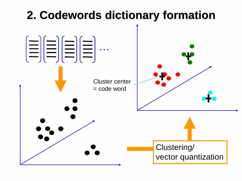
2. Codewords dictionary formation

Clustering/

vector quantization

…

Cluster center

= code word

2. Codewords dictionary formation

Fei-Fei et al. 2005

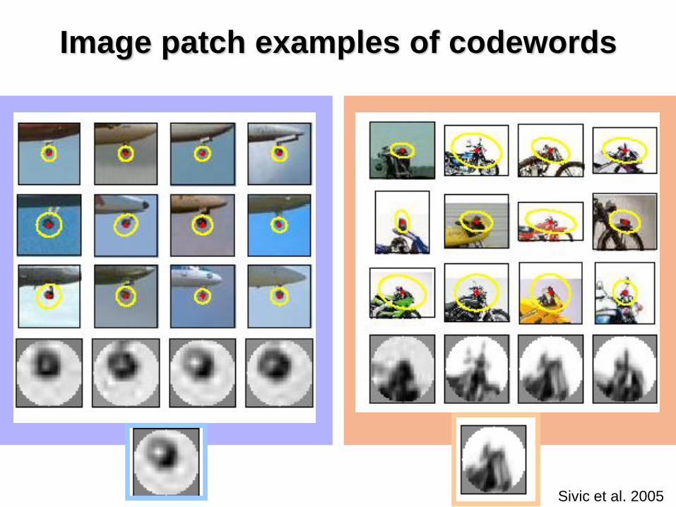
Image patch examples of codewords

Sivic et al. 2005

Visual vocabularies: Issues

• How to choose vocabulary size?

– Too small: visual words not representative of all patches

– Too large: quantization artifacts, overfitting

• Computational efficiency

– Vocabulary trees

(Nister & Stewenius, 2006)

3. Bag of word representation

Codewords dictionary • Nearest neighbors assignment

• K-D tree search strategy

3. Bag of word representation

Codewords dictionary

fre

qu

en

cy

codewords

….

• Texture is characterized by the repetition of basic

elements or textons

• For stochastic textures, it is the identity of the textons,

not their spatial arrangement, that matters

Julesz, 1981; Cula & Dana, 2001; Leung & Malik 2001; Mori, Belongie & Malik, 2001; Schmid 2001; Varma &

Zisserman, 2002, 2003; Lazebnik, Schmid & Ponce, 2003

Representing textures

Credit slide: S. Lazebnik

Universal texton dictionary

histogram

Julesz, 1981; Cula & Dana, 2001; Leung & Malik 2001; Mori, Belongie & Malik, 2001; Schmid 2001; Varma &

Zisserman, 2002, 2003; Lazebnik, Schmid & Ponce, 2003 Credit slide: S. Lazebnik

Representing textures

feature detection

& representation

codewords dictionary

image representation

Representation

1.

2.

3.

category models

Invariance issues

• Scale – rotation – view point - occlusions

– Implicit

– Detectors and descriptors

Kadir and Brady. 2003

Class 1 Class N

…

…

…

Category models

category

decision

codewords dictionary

category models

(and/or) classifiers

Learning and Recognition

category models

(and/or) classifiers

Learning and Recognition

1. Discriminative method:

- NN

- SVM

2.Generative method:

- graphical models

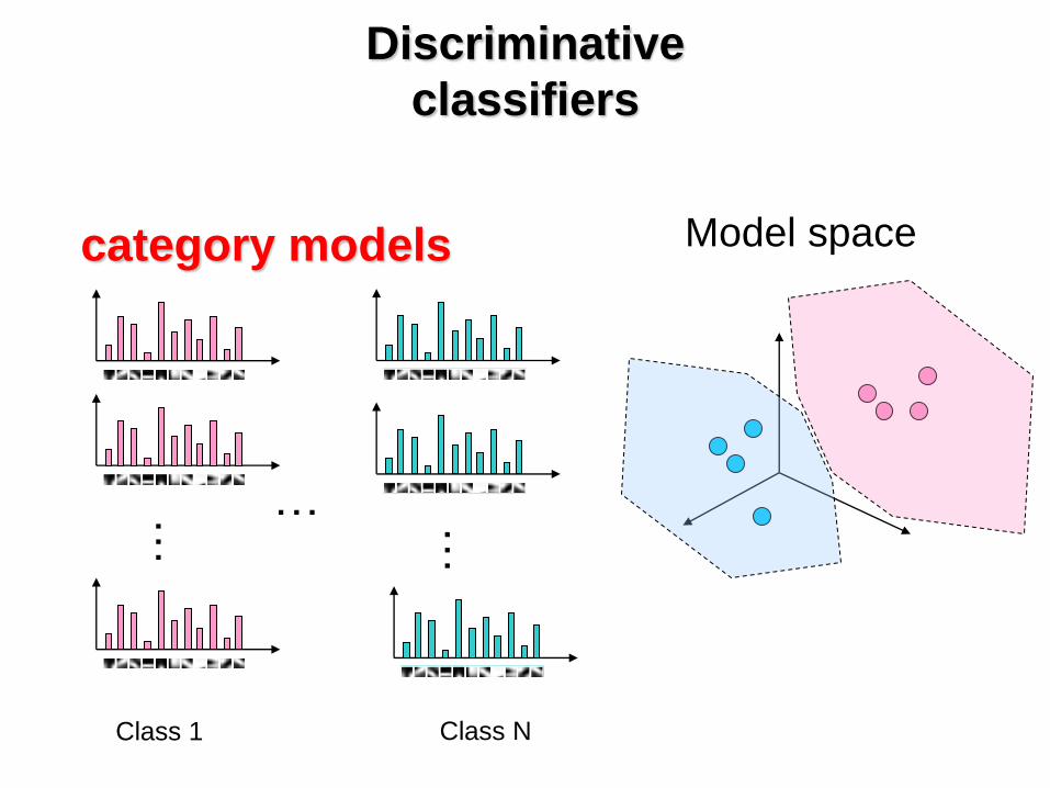
category models

Class 1 Class N

…

…

…

Discriminative

classifiers

Model space

Discriminative

classifiers

Query image

Winning class: pink

Model space

Nearest Neighbors

classifier

Query image

Winning class: pink

• Assign label of nearest training data point to

each test data point

Model space

Query image

Winning class: pink

• For a new point, find the k closest points from training data • Labels of the k points “vote” to classify • Works well provided there is lots of data and the distance function is good

K- Nearest Neighbors

classifier

Model space

• For k dimensions: k-D tree = space-partitioning data structure for organizing

points in a k-dimensional space

• Enable efficient search

from Duda et al.

K- Nearest Neighbors

classifier

• Voronoi partitioning of feature space for 2-category 2-D and 3-D data

• Nice tutorial: http://www.cs.umd.edu/class/spring2002/cmsc420-0401/pbasic.pdf

Functions for comparing

histograms • L1 distance

• χ2 distance

• Quadratic distance (cross-bin)

N

i

ihihhhD1

2121 |)()(|),(

Jan Puzicha, Yossi Rubner, Carlo Tomasi, Joachim M. Buhmann: Empirical Evaluation of

Dissimilarity Measures for Color and Texture. ICCV 1999

N

i ihih

ihihhhD

1 21

2

2121

)()(

)()(),(

ji

ij jhihAhhD,

2

2121 ))()((),(

Learning and Recognition

1. Discriminative method:

- NN

- SVM

2.Generative method:

- graphical models

Discriminative classifiers

(linear classifier)

Model space category models

Class 1 Class N

…

…

…

Linear classifiers • Find linear function (hyperplane) to separate

positive and negative examples

0:negative

0:positive

b

b

ii

ii

wxx

wxx

Which hyperplane

is best?

w, b

Support vector machines • Find hyperplane that maximizes the margin between the positive

and negative examples

Margin

Support vectors

Distance between point

and hyperplane: ||||

||

w

wx bi

Support vectors: 1 bi wx

Margin = 2 / ||w||

Credit slide: S. Lazebnik

i iii y xw

bybi iii xxxw

Classification function (decision boundary):

Solution:

Support vector machines • Classification

Margin

bybi iii xxxw

20

10

classbif

classbif

wx

wx

Test point

C. Burges, A Tutorial on Support Vector Machines for Pattern Recognition, Data Mining and Knowledge

Discovery, 1998

• Datasets that are linearly separable work out great:

•

•

• But what if the dataset is just too hard?

• We can map it to a higher-dimensional space:

0 x

0 x

0 x

x2

Nonlinear SVMs

Slide credit: Andrew Moore

Φ: x → φ(x)

Nonlinear SVMs

• General idea: the original input space can always be

mapped to some higher-dimensional feature space

where the training set is separable:

Slide credit: Andrew Moore

lifting transformation

Nonlinear SVMs

• Nonlinear decision boundary in the original

feature space:

bKyi

iii ),( xx

C. Burges, A Tutorial on Support Vector Machines for Pattern Recognition, Data Mining and Knowledge

Discovery, 1998

•The kernel K = product of the lifting transformation φ(x):

K(xi , xjj) = φ(xi ) · φ(xj)

NOTE:

• It is not required to compute φ(x) explicitly:

• The kernel must satisfy the “Mercer inequality”

Kernels for bags of features

• Histogram intersection kernel:

• Generalized Gaussian kernel:

• D can be Euclidean distance, χ2 distance etc…

N

i

ihihhhI1

2121 ))(),(min(),(

2

2121 ),(1

exp),( hhDA

hhK

J. Zhang, M. Marszalek, S. Lazebnik, and C. Schmid, Local Features and Kernels for Classifcation of Texture and

Object Categories: A Comprehensive Study, IJCV 2007

What about multi-class SVMs?

• No “definitive” multi-class SVM formulation

• In practice, we have to obtain a multi-class SVM by

combining multiple two-class SVMs

• One vs. others

– Traning: learn an SVM for each class vs. the others

– Testing: apply each SVM to test example and assign to it the

class of the SVM that returns the highest decision value

• One vs. one

– Training: learn an SVM for each pair of classes

– Testing: each learned SVM “votes” for a class to assign to the

test example

Credit slide: S. Lazebnik

SVMs: Pros and cons

• Pros

– Many publicly available SVM packages:

http://www.kernel-machines.org/software

– Kernel-based framework is very powerful, flexible

– SVMs work very well in practice, even with very small training sample

sizes

• Cons

– No “direct” multi-class SVM, must combine two-class SVMs

– Computation, memory

• During training time, must compute matrix of kernel values for every pair

of examples

• Learning can take a very long time for large-scale problems

Object recognition results

• ETH-80 database

8 object classes (Eichhorn and Chapelle 2004)

• Features:

– Harris detector

– PCA-SIFT descriptor, d=10

Kernel Complexity Recognition rate

Match [Wallraven et al.] 84%

Bhattacharyya affinity

[Kondor & Jebara] 85%

Pyramid match 84%

Slide credit: Kristen Grauman

Pyramid match kernel • Fast approximation of Earth Mover’s Distance

• Weighted sum of histogram intersections at mutliple resolutions

(linear in the number of features instead of cubic)

K. Grauman and T. Darrell. The Pyramid Match Kernel: Discriminative Classification with Sets of Image Features,

ICCV 2005.

Spatial Pyramid Matching

Beyond Bags of Features: Spatial Pyramid Matching for Recognizing Natural Scene Categories. S. Lazebnik, C. Schmid, and J. Ponce.

Proceedings of the IEEE Conference on Computer Vision and Pattern Recognition, New York, June 2006, vol. II, pp. 2169-2178.

Discriminative models

Support Vector Machines

Guyon, Vapnik, Heisele,

Serre, Poggio…

Boosting

Viola, Jones 2001,

Torralba et al. 2004,

Opelt et al. 2006,…

106 examples

Nearest neighbor

Shakhnarovich, Viola, Darrell 2003

Berg, Berg, Malik 2005...

Neural networks

Slide adapted from Antonio Torralba Courtesy of Vittorio Ferrari

Slide credit: Kristen Grauman

Latent SVM

Structural SVM

Felzenszwalb 00

Ramanan 03…

LeCun, Bottou, Bengio, Haffner 1998

Rowley, Baluja, Kanade 1998

…

Learning and Recognition

1. Discriminative method:

- NN

- SVM

2.Generative method:

- graphical models

Model the probability distribution that produces a given

bag of features

Generative models

1. Naïve Bayes classifier – Csurka Bray, Dance & Fan, 2004

2. Hierarchical Bayesian text models (pLSA and LDA)

– Background: Hoffman 2001, Blei, Ng & Jordan, 2004

– Object categorization: Sivic et al. 2005, Sudderth et al. 2005

– Natural scene categorization: Fei-Fei et al. 2005

Object categorization:

the statistical viewpoint

• Bayes rule:

)(

)(

)|(

)|(

)|(

)|(

zebranop

zebrap

zebranoimagep

zebraimagep

imagezebranop

imagezebrap

posterior ratio likelihood ratio prior ratio

• Discriminative methods model posterior

• Generative methods model likelihood and

prior

• w: a collection of all N codewords in the

image

w = [w1,w2,…,wN]

• c: category of the image

Some notations

the Naïve Bayes model

)c|w(p)c(p~

Prior prob. of

the object classes

Image likelihood

given the class

)w|c(p

w

N

c

)|,,()( 1 cwwpcp N

the Naïve Bayes model

)c|w(p)c(p~

Prior prob. of

the object classes

Image likelihood

given the class

)w|c(p )|,,()( 1 cwwpcp N

N

1i

i )c|w(p

• Assume that each feature (codewords) is conditionally

independent given the class

)c|w,,w(p N1

N

n

n cwpcp1

)|()(

Likelihood of nth visual

word given the class

the Naïve Bayes model

)c|w(p)c(p~

Prior prob. of

the object classes

Image likelihood

given the class

)w|c(p )|,,()( 1 cwwpcp N

N

n

n cwpcp1

)|()(

Likelihood of nth visual

word given the class

Classification/Recognition

)|()( cwpcp

N

n

n cwpcp1

)|()(

Object class

decision

)|( wcpc

c maxarg

)|( 1cwp i

)|( 2cwp i

• How do we learn P(wi|cj)?

• From empirical

frequencies of code words

in images from a given

class

Csurka et al. 2004

E = 28%

E = 15%

Summary: Generative models

• Naïve Bayes

– Unigram models in document analysis

– Assumes conditional independence of words given class

– Parameter estimation: frequency counting

Other generative BoW models

• Hierarchical Bayesian topic models (e.g. pLSA and LDA)

– Object categorization: Sivic et al. 2005, Sudderth et al. 2005

– Natural scene categorization: Fei-Fei et al. 2005

Generative vs discriminative

• Discriminative methods – Computationally efficient & fast

• Generative models – Convenient for weakly- or un-supervised,

incremental training

– Prior information

– Flexibility in modeling parameters

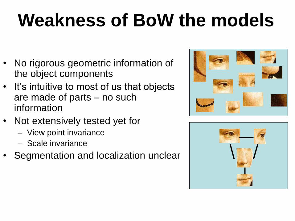
• No rigorous geometric information of the object components

• It’s intuitive to most of us that objects are made of parts – no such information

• Not extensively tested yet for – View point invariance

– Scale invariance

• Segmentation and localization unclear

Weakness of BoW the models

EECS 442 – Computer vision

Object Recognition

• Intro

• Recognition of 3D objects

• Recognition of object categories:

• Bag of world models

• Part based models

• 3D object categorization