ee-559 { deep learning 9. autoencoders and generative models · 2018-05-17 · many applications...
TRANSCRIPT

EE-559 – Deep learning
9. Autoencoders and generative models
Francois Fleuret
https://fleuret.org/dlc/
[version of: May 17, 2018]
ÉCOLE POLYTECHNIQUEFÉDÉRALE DE LAUSANNE

Embeddings and generative models
Francois Fleuret EE-559 – Deep learning / 9. Autoencoders and generative models 2 / 80

Many applications such as image synthesis, denoising, super-resolution, speechsynthesis, compression, etc. require to go beyond classification and regression,and model explicitly a high dimension signal.
This modeling consists of finding “meaningful degrees of freedom” that describethe signal, and are of lesser dimension.
Francois Fleuret EE-559 – Deep learning / 9. Autoencoders and generative models 3 / 80

Original space X
Latent space F
f
g
Francois Fleuret EE-559 – Deep learning / 9. Autoencoders and generative models 4 / 80

Original space X
Latent space F
f
g
Francois Fleuret EE-559 – Deep learning / 9. Autoencoders and generative models 4 / 80

Original space X
Latent space F
f
g
Francois Fleuret EE-559 – Deep learning / 9. Autoencoders and generative models 4 / 80

Original space X
Latent space F
f
g
Francois Fleuret EE-559 – Deep learning / 9. Autoencoders and generative models 4 / 80

Original space X
Latent space F
f
g
Francois Fleuret EE-559 – Deep learning / 9. Autoencoders and generative models 4 / 80

Original space X
Latent space F
f
g
Francois Fleuret EE-559 – Deep learning / 9. Autoencoders and generative models 4 / 80

Original space X
Latent space F
f
g
Francois Fleuret EE-559 – Deep learning / 9. Autoencoders and generative models 4 / 80

When dealing with real-world signals, this objective involves the sametheoretical and practical issues as for classification or regression: defining theright class of high-dimension models, and optimizing them.
Regarding synthesis, we saw that deep feed-forward architectures exhibit goodgenerative properties, which motivates their use explicitly for that purpose.
Francois Fleuret EE-559 – Deep learning / 9. Autoencoders and generative models 5 / 80

Autoencoders
Francois Fleuret EE-559 – Deep learning / 9. Autoencoders and generative models 6 / 80

An autoencoder combines an encoder f that embeds the original space X intoa latent space of lower dimension F, and a decoder g to map back to X, suchthat their composition g ◦ f is [close to] the identity on the data.
Original space X
Latent space F
f
g
A proper autoencoder has to capture a “good” parametrization of the signal,and in particular the statistical dependencies between the signal components.
Francois Fleuret EE-559 – Deep learning / 9. Autoencoders and generative models 7 / 80

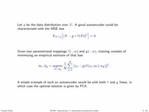
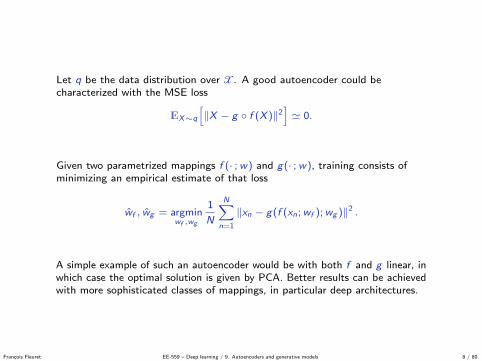
Let q be the data distribution over X. A good autoencoder could becharacterized with the MSE loss
EX∼q
[‖X − g ◦ f (X )‖2
]' 0.
Given two parametrized mappings f (· ;w) and g(· ;w), training consists ofminimizing an empirical estimate of that loss
wf , wg = argminwf ,wg
1
N
N∑n=1
‖xn − g(f (xn;wf );wg )‖2 .
A simple example of such an autoencoder would be with both f and g linear, inwhich case the optimal solution is given by PCA. Better results can be achievedwith more sophisticated classes of mappings, in particular deep architectures.
Francois Fleuret EE-559 – Deep learning / 9. Autoencoders and generative models 8 / 80
Let q be the data distribution over X. A good autoencoder could becharacterized with the MSE loss
EX∼q
[‖X − g ◦ f (X )‖2
]' 0.
Given two parametrized mappings f (· ;w) and g(· ;w), training consists ofminimizing an empirical estimate of that loss
wf , wg = argminwf ,wg
1
N
N∑n=1
‖xn − g(f (xn;wf );wg )‖2 .
A simple example of such an autoencoder would be with both f and g linear, inwhich case the optimal solution is given by PCA.
Better results can be achievedwith more sophisticated classes of mappings, in particular deep architectures.
Francois Fleuret EE-559 – Deep learning / 9. Autoencoders and generative models 8 / 80
Let q be the data distribution over X. A good autoencoder could becharacterized with the MSE loss
EX∼q
[‖X − g ◦ f (X )‖2
]' 0.
Given two parametrized mappings f (· ;w) and g(· ;w), training consists ofminimizing an empirical estimate of that loss
wf , wg = argminwf ,wg
1
N
N∑n=1
‖xn − g(f (xn;wf );wg )‖2 .
A simple example of such an autoencoder would be with both f and g linear, inwhich case the optimal solution is given by PCA. Better results can be achievedwith more sophisticated classes of mappings, in particular deep architectures.
Francois Fleuret EE-559 – Deep learning / 9. Autoencoders and generative models 8 / 80

Transposed convolutions
Francois Fleuret EE-559 – Deep learning / 9. Autoencoders and generative models 9 / 80

Constructing deep generative architectures, such as the decoder of anautoencoder, requires layers to increase the signal dimension, the contrary ofwhat we have done so far with feed-forward networks.
Generative processes that consist of optimizing the input rely onback-propagation to expend the signal from a low-dimension representation tothe high-dimension signal space.
The same can be done in the forward pass with transposed convolution layerswhose forward operation corresponds to a convolution layer backward pass.
Francois Fleuret EE-559 – Deep learning / 9. Autoencoders and generative models 10 / 80

Consider a 1d convolution with a kernel κ
yi = (x ~ κ)i
=∑a
xi+a−1 κa
=∑u
xu κu−i+1.
We get [∂l
∂x
]u
=∂l
∂xu
=∑i
∂l
∂yi
∂yi
∂xu
=∑i
∂l
∂yiκu−i+1.
which looks a lot like a standard convolution layer, except that the kernelcoefficients are visited in reverse order.
Francois Fleuret EE-559 – Deep learning / 9. Autoencoders and generative models 11 / 80

This is actually the standard convolution operator from signal processing. If ∗denotes this operation, we have
(x ∗ κ)i =∑a
xa κi−a+1.
Coming back to the backward pass of the convolution layer, if
y = x ~ κ
then [∂l
∂x
]=
[∂l
∂y
]∗ κ.
Francois Fleuret EE-559 – Deep learning / 9. Autoencoders and generative models 12 / 80

In the deep-learning field, since it corresponds to transposing the weight matrixof the equivalent fully-connected layer, it is called a transposed convolution.
κ1 κ2 κ3 0 0 0 00 κ1 κ2 κ3 0 0 00 0 κ1 κ2 κ3 0 00 0 0 κ1 κ2 κ3 00 0 0 0 κ1 κ2 κ3
T
=
κ1 0 0 0 0κ2 κ1 0 0 0κ3 κ2 κ1 0 00 κ3 κ2 κ1 00 0 κ3 κ2 κ1
0 0 0 κ3 κ2
0 0 0 0 κ3
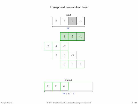
While a convolution can be seen as a series of inner products, a transposedconvolution can be seen as a weighted sum of translated kernels.
Francois Fleuret EE-559 – Deep learning / 9. Autoencoders and generative models 13 / 80

In the deep-learning field, since it corresponds to transposing the weight matrixof the equivalent fully-connected layer, it is called a transposed convolution.
κ1 κ2 κ3 0 0 0 00 κ1 κ2 κ3 0 0 00 0 κ1 κ2 κ3 0 00 0 0 κ1 κ2 κ3 00 0 0 0 κ1 κ2 κ3
T
=
κ1 0 0 0 0κ2 κ1 0 0 0κ3 κ2 κ1 0 00 κ3 κ2 κ1 00 0 κ3 κ2 κ1
0 0 0 κ3 κ2
0 0 0 0 κ3
While a convolution can be seen as a series of inner products, a transposedconvolution can be seen as a weighted sum of translated kernels.
Francois Fleuret EE-559 – Deep learning / 9. Autoencoders and generative models 13 / 80
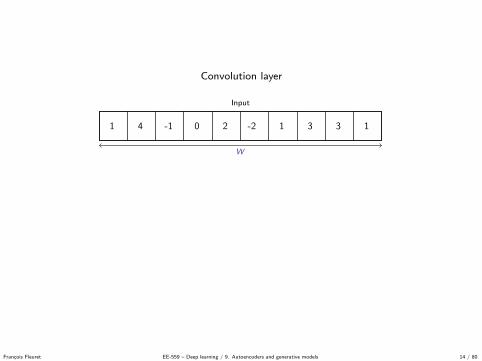
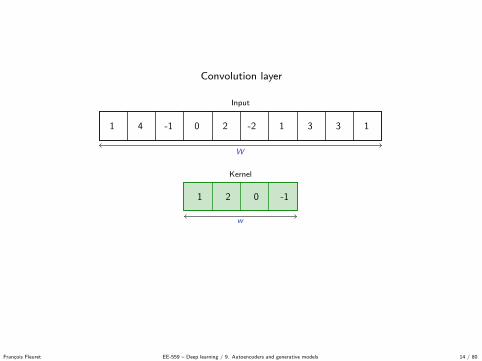
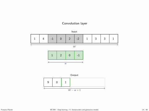
Convolution layer
Output
W − w + 1
1 2 0 -1
w
9
1 2 0 -1
w
0
1 2 0 -1
w
1
1 2 0 -1
w
3
1 2 0 -1
w
-5
1 2 0 -1
w
-3
1 2 0 -1
w
6
1 4 -1 0 2 -2 1 3 3 1
Input
W
Kernel
w
1 2 0 -1
Francois Fleuret EE-559 – Deep learning / 9. Autoencoders and generative models 14 / 80
Convolution layer
Output
W − w + 1
1 2 0 -1
w
9
1 2 0 -1
w
0
1 2 0 -1
w
1
1 2 0 -1
w
3
1 2 0 -1
w
-5
1 2 0 -1
w
-3
1 2 0 -1
w
6
1 4 -1 0 2 -2 1 3 3 1
Input
W
Kernel
w
1 2 0 -1
Francois Fleuret EE-559 – Deep learning / 9. Autoencoders and generative models 14 / 80

Convolution layer
Output
W − w + 1
1 2 0 -1
w
9
1 2 0 -1
w
0
1 2 0 -1
w
1
1 2 0 -1
w
3
1 2 0 -1
w
-5
1 2 0 -1
w
-3
1 2 0 -1
w
6
1 4 -1 0 2 -2 1 3 3 1
Input
W
Kernel
w
1 2 0 -1
Francois Fleuret EE-559 – Deep learning / 9. Autoencoders and generative models 14 / 80

Convolution layer
Output
W − w + 1
1 2 0 -1
w
9
1 2 0 -1
w
0
1 2 0 -1
w
1
1 2 0 -1
w
3
1 2 0 -1
w
-5
1 2 0 -1
w
-3
1 2 0 -1
w
6
1 4 -1 0 2 -2 1 3 3 1
Input
W
Kernel
w
1 2 0 -1
Francois Fleuret EE-559 – Deep learning / 9. Autoencoders and generative models 14 / 80
Convolution layer
Output
W − w + 1
1 2 0 -1
w
9
1 2 0 -1
w
0
1 2 0 -1
w
1
1 2 0 -1
w
3
1 2 0 -1
w
-5
1 2 0 -1
w
-3
1 2 0 -1
w
6
1 4 -1 0 2 -2 1 3 3 1
Input
W
Kernel
w
1 2 0 -1
Francois Fleuret EE-559 – Deep learning / 9. Autoencoders and generative models 14 / 80

Convolution layer
Output
W − w + 1
1 2 0 -1
w
9
1 2 0 -1
w
0
1 2 0 -1
w
1
1 2 0 -1
w
3
1 2 0 -1
w
-5
1 2 0 -1
w
-3
1 2 0 -1
w
6
1 4 -1 0 2 -2 1 3 3 1
Input
W
Kernel
w
1 2 0 -1
Francois Fleuret EE-559 – Deep learning / 9. Autoencoders and generative models 14 / 80

Convolution layer
Output
W − w + 1
1 2 0 -1
w
9
1 2 0 -1
w
0
1 2 0 -1
w
1
1 2 0 -1
w
3
1 2 0 -1
w
-5
1 2 0 -1
w
-3
1 2 0 -1
w
6
1 4 -1 0 2 -2 1 3 3 1
Input
W
Kernel
w
1 2 0 -1
Francois Fleuret EE-559 – Deep learning / 9. Autoencoders and generative models 14 / 80

Convolution layer
Output
W − w + 1
1 2 0 -1
w
9
1 2 0 -1
w
0
1 2 0 -1
w
1
1 2 0 -1
w
3
1 2 0 -1
w
-5
1 2 0 -1
w
-3
1 2 0 -1
w
6
1 4 -1 0 2 -2 1 3 3 1
Input
W
Kernel
w
1 2 0 -1
Francois Fleuret EE-559 – Deep learning / 9. Autoencoders and generative models 14 / 80

Convolution layer
Output
W − w + 1
1 2 0 -1
w
9
1 2 0 -1
w
0
1 2 0 -1
w
1
1 2 0 -1
w
3
1 2 0 -1
w
-5
1 2 0 -1
w
-3
1 2 0 -1
w
6
1 4 -1 0 2 -2 1 3 3 1
Input
W
Kernel
w
1 2 0 -1
Francois Fleuret EE-559 – Deep learning / 9. Autoencoders and generative models 14 / 80

Convolution layer
Output
W − w + 1
1 2 0 -1
w
9
1 2 0 -1
w
0
1 2 0 -1
w
1
1 2 0 -1
w
3
1 2 0 -1
w
-5
1 2 0 -1
w
-3
1 2 0 -1
w
6
1 4 -1 0 2 -2 1 3 3 1
Input
W
Kernel
w
1 2 0 -1
Francois Fleuret EE-559 – Deep learning / 9. Autoencoders and generative models 14 / 80

Transposed convolution layer
Output
W + w − 1
1 2 -11 2 -11 2 -11 2 -1
1 2 -1
Kernel
w
2 4 -2
3 6 -3
0 0 0
-1 -2 1
Input
W
2 3 0 -1
2 7 4 -4 -2 1
Francois Fleuret EE-559 – Deep learning / 9. Autoencoders and generative models 15 / 80

Transposed convolution layer
Output
W + w − 1
1 2 -1
1 2 -11 2 -11 2 -1
1 2 -1
Kernel
w
2 4 -2
3 6 -3
0 0 0
-1 -2 1
Input
W
2 3 0 -1
2
7 4 -4 -2 1
Francois Fleuret EE-559 – Deep learning / 9. Autoencoders and generative models 15 / 80

Transposed convolution layer
Output
W + w − 1
1 2 -1
1 2 -1
1 2 -11 2 -1
1 2 -1
Kernel
w
2 4 -2
3 6 -3
0 0 0
-1 -2 1
Input
W
2 3 0 -1
2 7
4 -4 -2 1
Francois Fleuret EE-559 – Deep learning / 9. Autoencoders and generative models 15 / 80
Transposed convolution layer
Output
W + w − 1
1 2 -11 2 -1
1 2 -1
1 2 -1
1 2 -1
Kernel
w
2 4 -2
3 6 -3
0 0 0
-1 -2 1
Input
W
2 3 0 -1
2 7 4
-4 -2 1
Francois Fleuret EE-559 – Deep learning / 9. Autoencoders and generative models 15 / 80

Transposed convolution layer
Output
W + w − 1
1 2 -11 2 -11 2 -1
1 2 -1
1 2 -1
Kernel
w
2 4 -2
3 6 -3
0 0 0
-1 -2 1
Input
W
2 3 0 -1
2 7 4 -4 -2 1
Francois Fleuret EE-559 – Deep learning / 9. Autoencoders and generative models 15 / 80

Transposed convolution layer
Output
W + w − 1
1 2 -11 2 -11 2 -11 2 -1
1 2 -1
Kernel
w
2 4 -2
3 6 -3
0 0 0
-1 -2 1
Input
W
2 3 0 -1
2 7 4 -4 -2 1
Francois Fleuret EE-559 – Deep learning / 9. Autoencoders and generative models 15 / 80

Transposed convolution layer
Output
W + w − 1
1 2 -11 2 -11 2 -11 2 -1
1 2 -1
Kernel
w
2 4 -2
3 6 -3
0 0 0
-1 -2 1
Input
W
2 3 0 -1
2 7 4 -4 -2 1
Francois Fleuret EE-559 – Deep learning / 9. Autoencoders and generative models 15 / 80
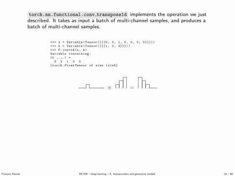
torch.nn.functional.conv transpose1d implements the operation we justdescribed. It takes as input a batch of multi-channel samples, and produces abatch of multi-channel samples.
>>> x = Variable(Tensor ([[[0 , 0, 1, 0, 0, 0, 0]]]))
>>> k = Variable(Tensor ([[[1 , 2, 3]]]))
>>> F.conv1d(x, k)
Variable containing:
(0 ,.,.) =
3 2 1 0 0
[torch.FloatTensor of size 1x1x5]
~ =
>>> F.conv_transpose1d(x, k)
Variable containing:
(0 ,.,.) =
0 0 1 2 3 0 0 0 0
[torch.FloatTensor of size 1x1x9]
∗ =
Francois Fleuret EE-559 – Deep learning / 9. Autoencoders and generative models 16 / 80

The class torch.nn.ConvTranspose1d implements that operation into a
torch.nn.Module .
>>> x = Variable(Tensor ([[[ 2, 3, 0, -1]]]))
>>> m = nn.ConvTranspose1d (1, 1, kernel_size =3)
>>> m.bias.data.zero_ ()
0
[torch.FloatTensor of size 1]
>>> m.weight.data.copy_(Tensor ([ 1, 2, -1 ]))
(0 ,.,.) =
1 2 -1
[torch.FloatTensor of size 1x1x3]
>>> y = m(x)
>>> y
Variable containing:
(0 ,.,.) =
2 7 4 -4 -2 1
[torch.FloatTensor of size 1x1x6]
Francois Fleuret EE-559 – Deep learning / 9. Autoencoders and generative models 17 / 80

Transposed convolutions also have a dilation parameter that behaves as forconvolution and expends the kernel size without increasing the number ofparameters by making it sparse.
They also have a stride and padding parameters, however, due to therelation between convolutions and transposed convolutions:
BWhile for convolutions stride and padding are defined in the inputmap, for transposed convolutions these parameters are defined in theoutput map, and the latter modulates a cropping operation.
Francois Fleuret EE-559 – Deep learning / 9. Autoencoders and generative models 18 / 80

Transposed convolution layer (stride = 2)
Output
s(W − 1) + w
1 2 -11 2 -11 2 -11 2 -1
1 2 -1
Kernel
w
2 4 -2
3 6 -3s
0 0 0s
-1 -2 1s
Input
W
2 3 0 -1
2 4 1 6 -3 0 -1 -2 1
Francois Fleuret EE-559 – Deep learning / 9. Autoencoders and generative models 19 / 80

Transposed convolution layer (stride = 2)
Output
s(W − 1) + w
1 2 -1
1 2 -11 2 -11 2 -1
1 2 -1
Kernel
w
2 4 -2
3 6 -3s
0 0 0s
-1 -2 1s
Input
W
2 3 0 -1
2 4
1 6 -3 0 -1 -2 1
Francois Fleuret EE-559 – Deep learning / 9. Autoencoders and generative models 19 / 80

Transposed convolution layer (stride = 2)
Output
s(W − 1) + w
1 2 -1
1 2 -1
1 2 -11 2 -1
1 2 -1
Kernel
w
2 4 -2
3 6 -3s
0 0 0s
-1 -2 1s
Input
W
2 3 0 -1
2 4 1 6
-3 0 -1 -2 1
Francois Fleuret EE-559 – Deep learning / 9. Autoencoders and generative models 19 / 80

Transposed convolution layer (stride = 2)
Output
s(W − 1) + w
1 2 -11 2 -1
1 2 -1
1 2 -1
1 2 -1
Kernel
w
2 4 -2
3 6 -3s
0 0 0s
-1 -2 1s
Input
W
2 3 0 -1
2 4 1 6 -3 0
-1 -2 1
Francois Fleuret EE-559 – Deep learning / 9. Autoencoders and generative models 19 / 80

Transposed convolution layer (stride = 2)
Output
s(W − 1) + w
1 2 -11 2 -11 2 -1
1 2 -1
1 2 -1
Kernel
w
2 4 -2
3 6 -3s
0 0 0s
-1 -2 1s
Input
W
2 3 0 -1
2 4 1 6 -3 0 -1 -2 1
Francois Fleuret EE-559 – Deep learning / 9. Autoencoders and generative models 19 / 80

Transposed convolution layer (stride = 2)
Output
s(W − 1) + w
1 2 -11 2 -11 2 -11 2 -1
1 2 -1
Kernel
w
2 4 -2
3 6 -3s
0 0 0s
-1 -2 1s
Input
W
2 3 0 -1
2 4 1 6 -3 0 -1 -2 1
Francois Fleuret EE-559 – Deep learning / 9. Autoencoders and generative models 19 / 80

Transposed convolution layer (stride = 2)
Output
s(W − 1) + w
1 2 -11 2 -11 2 -11 2 -1
1 2 -1
Kernel
w
2 4 -2
3 6 -3s
0 0 0s
-1 -2 1s
Input
W
2 3 0 -1
2 4 1 6 -3 0 -1 -2 1
Francois Fleuret EE-559 – Deep learning / 9. Autoencoders and generative models 19 / 80

The composition of a convolution and a transposed convolution of sameparameters keep the signal size [roughly] unchanged.
BA convolution with a stride greater than one may ignore parts of thesignal. Its composition with the corresponding transposed convolutiongenerates a map of the size of the observed area.
For instance, a 1d convolution of kernel size w and stride s composed with thetransposed convolution of same parameters maintains the signal size W , only if
∃q ∈ N, W = w + s q.
W
s s s w
Francois Fleuret EE-559 – Deep learning / 9. Autoencoders and generative models 20 / 80

It has been observed that transposed convolutions may create somegrid-structure artifact, since generated pixels are not all covered similarly.
For instance with a 4× 4 kernel and stride 3
Francois Fleuret EE-559 – Deep learning / 9. Autoencoders and generative models 21 / 80

An alternative is to use an analytic up-scaling. Two standard such PyTorchmodules are nn.UpsamplingBilinear2d and nn.Upsample .
>>> x = Variable(Tensor ([[[[ 1, 2 ], [ 3, 4 ]]]]))
>>> b = nn.UpsamplingBilinear2d(scale_factor = 3)
>>> b(x)
Variable containing:
(0 ,0 ,.,.) =
1.0000 1.2000 1.4000 1.6000 1.8000 2.0000
1.4000 1.6000 1.8000 2.0000 2.2000 2.4000
1.8000 2.0000 2.2000 2.4000 2.6000 2.8000
2.2000 2.4000 2.6000 2.8000 3.0000 3.2000
2.6000 2.8000 3.0000 3.2000 3.4000 3.6000
3.0000 3.2000 3.4000 3.6000 3.8000 4.0000
[torch.FloatTensor of size 1x1x6x6]
>>> u = nn.Upsample(scale_factor = 3, mode = ’nearest ’)
>>> u(x)
Variable containing:
(0 ,0 ,.,.) =
1 1 1 2 2 2
1 1 1 2 2 2
1 1 1 2 2 2
3 3 3 4 4 4
3 3 3 4 4 4
3 3 3 4 4 4
[torch.FloatTensor of size 1x1x6x6]
Francois Fleuret EE-559 – Deep learning / 9. Autoencoders and generative models 22 / 80

Such module is usually combined with a convolution to learn local correctionsto undesirable artifacts of the up-scaling.
In practice, a transposed convolution such as
nn.ConvTranspose2d(nic , noc ,
kernel_size = 3, stride = 2,
padding = 1, output_padding = 1),
can be replaced by
nn.UpsamplingBilinear2d(scale_factor = 2)
nn.Conv2d(nic , noc , kernel_size = 3, padding = 1)
or
nn.Upsample(scale_factor = 2, mode = ’nearest ’)
nn.Conv2d(nic , noc , kernel_size = 3, padding = 1)
Francois Fleuret EE-559 – Deep learning / 9. Autoencoders and generative models 23 / 80
Deep Autoencoders
Francois Fleuret EE-559 – Deep learning / 9. Autoencoders and generative models 24 / 80

A deep autoencoder combines an encoder composed of convolutional layers, anda decoder composed of the reciprocal transposed convolution layers.
To run a simple example on MNIST, we consider the following model, wheredimension reduction is obtained through filter sizes and strides > 1, avoidingmax-pooling layers.
AutoEncoder (
(encoder): Sequential (
(0): Conv2d(1, 32, kernel_size =(5, 5), stride =(1, 1))
(1): ReLU (inplace)
(2): Conv2d (32, 32, kernel_size =(5, 5), stride =(1, 1))
(3): ReLU (inplace)
(4): Conv2d (32, 32, kernel_size =(4, 4), stride =(2, 2))
(5): ReLU (inplace)
(6): Conv2d (32, 32, kernel_size =(3, 3), stride =(2, 2))
(7): ReLU (inplace)
(8): Conv2d (32, 8, kernel_size =(4, 4), stride =(1, 1))
)
(decoder): Sequential (
(0): ConvTranspose2d (8, 32, kernel_size =(4, 4), stride =(1, 1))
(1): ReLU (inplace)
(2): ConvTranspose2d (32, 32, kernel_size =(3, 3), stride =(2, 2))
(3): ReLU (inplace)
(4): ConvTranspose2d (32, 32, kernel_size =(4, 4), stride =(2, 2))
(5): ReLU (inplace)
(6): ConvTranspose2d (32, 32, kernel_size =(5, 5), stride =(1, 1))
(7): ReLU (inplace)
(8): ConvTranspose2d (32, 1, kernel_size =(5, 5), stride =(1, 1))
)
)
Francois Fleuret EE-559 – Deep learning / 9. Autoencoders and generative models 25 / 80

Encoder
Tensor sizes / operations
1×28×28
nn.Conv2d(1, 32, kernel size=5, stride=1)28
×2432×24×24
nn.Conv2d(32, 32, kernel size=5, stride=1)24
×2032×20×20
nn.Conv2d(32, 32, kernel size=4, stride=2)20
×932×9×9
nn.Conv2d(32, 32, kernel size=3, stride=2)9
×432×4×4
nn.Conv2d(32, 8, kernel size=4, stride=1)4
×18×1×1
Francois Fleuret EE-559 – Deep learning / 9. Autoencoders and generative models 26 / 80

Decoder
Tensor sizes / operations
8×1×1
nn.ConvTranspose2d(8, 32, kernel size=4, stride=1)×1
432×4×4
nn.ConvTranspose2d(32, 32, kernel size=3, stride=2)×4
332×9×9
nn.ConvTranspose2d(32, 32, kernel size=4, stride=2)×9
432×20×20
nn.ConvTranspose2d(32, 32, kernel size=5, stride=1)×20
532×24×24
nn.ConvTranspose2d(32, 1, kernel size=5, stride=1)×24
51×28×28
Francois Fleuret EE-559 – Deep learning / 9. Autoencoders and generative models 27 / 80

Training is achieved with MSE and Adam
model = AutoEncoder(embedding_dim , nb_channels)
mse_loss = nn.MSELoss ()
if torch.cuda.is_available ():
model.cuda()
mse_loss.cuda()
optimizer = optim.Adam(model.parameters (), lr = 1e-3)
for epoch in range(args.nb_epochs):
for input , _ in iter(train_loader):
if torch.cuda.is_available (): input = input.cuda()
input = Variable(input)
output = model(input)
loss = mse_loss(output , input)
model.zero_grad ()
loss.backward ()
optimizer.step()
Francois Fleuret EE-559 – Deep learning / 9. Autoencoders and generative models 28 / 80

X (original samples)
g ◦ f (X ) (CNN, d = 2)
g ◦ f (X ) (PCA, d = 2)
Francois Fleuret EE-559 – Deep learning / 9. Autoencoders and generative models 29 / 80

X (original samples)
g ◦ f (X ) (CNN, d = 4)
g ◦ f (X ) (PCA, d = 4)
Francois Fleuret EE-559 – Deep learning / 9. Autoencoders and generative models 29 / 80

X (original samples)
g ◦ f (X ) (CNN, d = 8)
g ◦ f (X ) (PCA, d = 8)
Francois Fleuret EE-559 – Deep learning / 9. Autoencoders and generative models 29 / 80

X (original samples)
g ◦ f (X ) (CNN, d = 16)
g ◦ f (X ) (PCA, d = 16)
Francois Fleuret EE-559 – Deep learning / 9. Autoencoders and generative models 29 / 80

X (original samples)
g ◦ f (X ) (CNN, d = 32)
g ◦ f (X ) (PCA, d = 32)
Francois Fleuret EE-559 – Deep learning / 9. Autoencoders and generative models 29 / 80

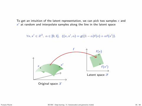
To get an intuition of the latent representation, we can pick two samples x andx ′ at random and interpolate samples along the line in the latent space
∀x , x ′ ∈ X2, α ∈ [0, 1], ξ(x , x ′, α) = g((1− α)f (x) + αf (x ′)).
Original space X
Latent space F
x x ′
f (x)
f (x ′)
f
g
Francois Fleuret EE-559 – Deep learning / 9. Autoencoders and generative models 30 / 80

Autoencoder interpolation (d = 8)
Francois Fleuret EE-559 – Deep learning / 9. Autoencoders and generative models 31 / 80

Autoencoder interpolation (d = 32)
Francois Fleuret EE-559 – Deep learning / 9. Autoencoders and generative models 32 / 80

And we can assess the generative capabilities of the decoder g by introducing a[simple] density model qZ over the latent space F, sample there, and map thesamples into the image space X with g .
We can for instance use a Gaussian model with diagonal covariance matrix.
f (X ) ∼ N(m, ∆)
where m is a vector and ∆ a diagonal matrix, both estimated on training data.
Original space X
Latent space F
g
Francois Fleuret EE-559 – Deep learning / 9. Autoencoders and generative models 33 / 80

Autoencoder sampling (d = 8)
Autoencoder sampling (d = 16)
Autoencoder sampling (d = 32)
Francois Fleuret EE-559 – Deep learning / 9. Autoencoders and generative models 34 / 80

These results are unsatisfying, because the density model used on the latentspace F is too simple and inadequate.
Building a “good” model amounts to our original problem of modeling anempirical distribution, although it may now be in a lower dimension space.
Francois Fleuret EE-559 – Deep learning / 9. Autoencoders and generative models 35 / 80

Denoising Autoencoders
Francois Fleuret EE-559 – Deep learning / 9. Autoencoders and generative models 36 / 80
Vincent et al. (2010) interpret the autoencoder in a probabilistic framework as away of building an encoder that maximizes the mutual information between theinput and the latent state.
Let X be a sample, Z = f (X ; θ) its latent representation, and qθ(x , z) thedistribution of (X ,Z).
We have
argmaxθ
I(X ,Z) = argmaxθ
H(X )−H(X | Z)
= argmaxθ
−H(X | Z)
= argmaxθ
E[
log qθ(X | Z)].
However, there is no expression of qθ(X | Z) in any reasonable setup.
Francois Fleuret EE-559 – Deep learning / 9. Autoencoders and generative models 37 / 80

For any distribution p we have
E[
log qθ(X | Z)]≥ E
[log p(X | Z)
].
So we can in particular approximate the left term with the right one byoptimizing a reconstruction model pη to make the inequality tight.
Francois Fleuret EE-559 – Deep learning / 9. Autoencoders and generative models 38 / 80

For any distribution p we have
E[
log qθ(X | Z)]≥ E
[log p(X | Z)
].
So we can in particular approximate the left term with the right one byoptimizing a reconstruction model pη to make the inequality tight.
Francois Fleuret EE-559 – Deep learning / 9. Autoencoders and generative models 38 / 80

If we consider the following model for p
pη ( · | Z = z) ∼ N(g(z), σ)
where g is deterministic,
we get
E[
log pη(X | Z)]
= −E[‖X − g(Z ; η)‖2
2σ2
]= −E
[‖X − g(f (X ; θ); η)‖2
2σ2
].
If optimizing η makes the bound tight, the final loss is the reconstruction error
argmaxθ
I(X ,Z) ' argminθ
(minη
1
N
N∑n=1
‖xn − g(f (xn; θ); η)‖2
)
This abstract view of the encoder as “maximizing information” justifies itsuse to build generic encoding layers.
Francois Fleuret EE-559 – Deep learning / 9. Autoencoders and generative models 39 / 80

If we consider the following model for p
pη ( · | Z = z) ∼ N(g(z), σ)
where g is deterministic, we get
E[
log pη(X | Z)]
= −E[‖X − g(Z ; η)‖2
2σ2
]= −E
[‖X − g(f (X ; θ); η)‖2
2σ2
].
If optimizing η makes the bound tight, the final loss is the reconstruction error
argmaxθ
I(X ,Z) ' argminθ
(minη
1
N
N∑n=1
‖xn − g(f (xn; θ); η)‖2
)
This abstract view of the encoder as “maximizing information” justifies itsuse to build generic encoding layers.
Francois Fleuret EE-559 – Deep learning / 9. Autoencoders and generative models 39 / 80

In the perspective of building a good feature representation, just retaininginformation is not enough, otherwise the identity would be a good choice.
Reducing dimension, or forcing sparsity is a way to push the model to maximizeretained information in a constraint coding space.
In their work, Vincent et al. proposed to degrade the signal with noise beforefeeding it to the encoder, but to keep the MSE to the original signal. Thisforces the encoder to retain meaningful structures.
Francois Fleuret EE-559 – Deep learning / 9. Autoencoders and generative models 40 / 80

V INCENT, LAROCHELLE, LAJOIE, BENGIO AND MANZAGOL
Figure 6: Weight decay vs. Gaussian noise. We show typical filters learnt from natural imagepatches in the over-complete case (200 hidden units).Left: regular autoencoder withweight decay. We tried a wide range of weight-decay values and learningrates: filtersnever appeared to capture a more interesting structure than what is shownhere. Notethat some local blob detectors are recovered compared to using no weightdecay at all(Figure 5 right).Right: a denoising autoencoder with additive Gaussian noise (σ = 0.5)learns Gabor-like local oriented edge detectors. Clearly the filters learntare qualitativelyvery different in the two cases.
yielded a mixture of edge detectors and grating filters. Clearly different corruption types and levelscan yield qualitatively different filters. But it is interesting to note that all three noise types weexperimented with were able to yield some potentially useful edge detectors.
5.2 Feature Detectors Learnt from Handwritten Digits
We also trained denoising autoencoders on the 28× 28 gray-scale images of handwritten digitsfrom the MNIST data set. For this experiment, we used denoising autoencoders with tied weights,cross-entropy reconstruction error, and zero-masking noise. The goal was to better understand thequalitative effect of the noise level. So we trained several denoising autoencoders, all starting fromthe same initial random point in weight space, butwith different noise levels.Figure 8 shows someof the resulting filters learnt and how they are affected as we increase thelevel of corruption. With0% corruption, the majority of the filters appear totally random, with only a few that specialize aslittle ink blob detectors. With increased noise levels, a much larger proportion of interesting (visiblynon random and with a clear structure) feature detectors are learnt. These include local orientedstroke detectors and detectors of digit parts such as loops. It was to be expected that denoising amore corrupted input requires detecting bigger, less local structures: the denoising auto-encodermust rely on longer range statistical dependencies and pool evidence from a larger subset of pixels.Interestingly, filters that start from the same initial random weight vector often look like they “grow”from random, to local blob detector, to slightly bigger structure detectors such as a stroke detector,as we use increased noise levels. By “grow” we mean that the slightly largerstructure learnt at ahigher noise level often appears related to the smaller structure obtained atlower noise levels, inthat they share about the same position and orientation.
3388
(Vincent et al., 2010)
Francois Fleuret EE-559 – Deep learning / 9. Autoencoders and generative models 41 / 80

STACKED DENOISING AUTOENCODERS
Figure 7: Filters obtained on natural image patches by denoising autoencoders using other noisetypes.Left: with 10% salt-and-pepper noise, we obtain oriented Gabor-like filters. Theyappear slightly less localized than when using Gaussian noise (contrast withFigure 6right). Right: with 55% zero-masking noise we obtain filters that look like orientedgratings. For the three considered noise types, denoising training appears to learn filtersthat capture meaningful natural image statistics structure.
6. Experiments on Stacked Denoising Autoencoders
In this section, we evaluate denoising autoencoders as a pretraining strategy for building deep net-works, using the stacking procedure that we described in Section 3.5. Weshall mainly compare theclassification performance of networks pretrained by stacking denoisingautoencoders (SDAE), ver-sus stacking regular autoencoders (SAE), versus stacking restrictedBoltzmann machines (DBN),on a benchmark of classification problems.
6.1 Considered Classification Problems and Experimental Methodology
We considered 10 classification problems, the details of which are listed in Table 1. They consistof:
• The standard MNIST digit classification problem with 60000 training examples.
• The eight benchmark image classification problems used in Larochelle et al. (2007) which in-clude more challenging variations of the MNIST digit classification problem (all with 10000training examples), as well as three artificial 28× 28 binary image classification tasks.11
These problems were designed to be particularly challenging to current generic learning al-gorithms (Larochelle et al., 2007). They are illustrated in Figure 9.
• A variation of thetzanetakisaudio genre classification data set (Bergstra, 2006) which con-tains 10000 three-second audio clips, equally distributed among 10 musical genres: blues,classical, country, disco, hiphop, pop, jazz, metal, reggae and rock. Each example in the set
11. The data sets for this benchmark are available athttp://www.iro.umontreal.ca/ ˜ lisa/icml2007 .
3389
(Vincent et al., 2010)
Francois Fleuret EE-559 – Deep learning / 9. Autoencoders and generative models 42 / 80

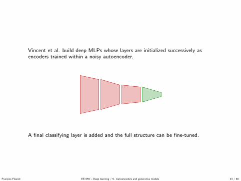
Vincent et al. build deep MLPs whose layers are initialized successively asencoders trained within a noisy autoencoder.
AutoencoderAutoencoderAutoencoder
A final classifying layer is added and the full structure can be fine-tuned.
Francois Fleuret EE-559 – Deep learning / 9. Autoencoders and generative models 43 / 80

Vincent et al. build deep MLPs whose layers are initialized successively asencoders trained within a noisy autoencoder.
Autoencoder
AutoencoderAutoencoder
A final classifying layer is added and the full structure can be fine-tuned.
Francois Fleuret EE-559 – Deep learning / 9. Autoencoders and generative models 43 / 80

Vincent et al. build deep MLPs whose layers are initialized successively asencoders trained within a noisy autoencoder.
AutoencoderAutoencoderAutoencoder
A final classifying layer is added and the full structure can be fine-tuned.
Francois Fleuret EE-559 – Deep learning / 9. Autoencoders and generative models 43 / 80

Vincent et al. build deep MLPs whose layers are initialized successively asencoders trained within a noisy autoencoder.
Autoencoder
Autoencoder
Autoencoder
A final classifying layer is added and the full structure can be fine-tuned.
Francois Fleuret EE-559 – Deep learning / 9. Autoencoders and generative models 43 / 80

Vincent et al. build deep MLPs whose layers are initialized successively asencoders trained within a noisy autoencoder.
AutoencoderAutoencoderAutoencoder
A final classifying layer is added and the full structure can be fine-tuned.
Francois Fleuret EE-559 – Deep learning / 9. Autoencoders and generative models 43 / 80

Vincent et al. build deep MLPs whose layers are initialized successively asencoders trained within a noisy autoencoder.
AutoencoderAutoencoder
Autoencoder
A final classifying layer is added and the full structure can be fine-tuned.
Francois Fleuret EE-559 – Deep learning / 9. Autoencoders and generative models 43 / 80

Vincent et al. build deep MLPs whose layers are initialized successively asencoders trained within a noisy autoencoder.
AutoencoderAutoencoderAutoencoder
A final classifying layer is added and the full structure can be fine-tuned.
Francois Fleuret EE-559 – Deep learning / 9. Autoencoders and generative models 43 / 80

V INCENT, LAROCHELLE, LAJOIE, BENGIO AND MANZAGOL
Data Set SVMrb f DBN-1 SAE-3 DBN-3 SDAE-3 (ν)
MNIST 1.40±0.23 1.21±0.21 1.40±0.23 1.24±0.22 1.28±0.22 (25%)basic 3.03±0.15 3.94±0.17 3.46±0.16 3.11±0.15 2.84±0.15 (10%)rot 11.11±0.28 14.69±0.31 10.30±0.27 10.30±0.27 9.53±0.26 (25%)bg-rand 14.58±0.31 9.80±0.26 11.28±0.28 6.73±0.22 10.30±0.27 (40%)bg-img 22.61±0.37 16.15±0.32 23.00±0.37 16.31±0.32 16.68±0.33 (25%)bg-img-rot 55.18±0.44 52.21±0.44 51.93±0.44 47.39±0.44 43.76±0.43 (25%)rect 2.15±0.13 4.71±0.19 2.41±0.13 2.60±0.14 1.99±0.12 (10%)rect-img 24.04±0.37 23.69±0.37 24.05±0.37 22.50±0.37 21.59±0.36 (25%)convex 19.13±0.34 19.92±0.35 18.41±0.34 18.63±0.34 19.06±0.34 (10%)tzanetakis 14.41±2.18 18.07±1.31 16.15±1.95 18.38±1.64 16.02±1.04(0.05)
Table 3: Comparison of stacked denoising autoencoders (SDAE-3) with other models. Test errorrate on all considered classification problems is reported together with a 95%confidenceinterval. Best performer is in bold, as well as those for which confidenceintervals overlap.SDAE-3 appears to achieve performance superior or equivalent to thebest other model onall problems exceptbg-rand. For SDAE-3, we also indicate the fractionν of corruptedinput components, or in case oftzanetakis, the standard deviation of the Gaussian noise, aschosen by proper model selection. Note that SAE-3 is equivalent to SDAE-3 with ν = 0%.
grained series of experiments, we chose to concentrate on the hardest of the considered problems,that is, the one with the most factors of variation:bg-img-rot.
We first examine how the proposed network training strategy behaves as we increase the capacityof the model both in breadth (number of neurons per layer) and in depth (number of hidden layers).Figure 10 shows the evolution of the performance as we increase the number of hidden layers from1 to 3, for three different network training strategies: without any pretraining (standard MLP),with ordinary autoencoder pretraining (SAE) and with denoising autoencoder pretraining (SDAE).We clearly see a strict ordering: denoising pretraining being better than autoencoder pretrainingbeing better than no pretraining. The advantage appears to increase with the number of layers (notethat without pretraining it seems impossible to successfully train a 3 hidden layer network) andwith the number of hidden units. This general behavior is a typical illustration of what is gainedby pretraining deep networks with a good unsupervised criterion, and appears to be common toseveral pretraining strategies. We refer the reader to Erhan et al. (2010) for an empirical studyand discussion regarding possible explanations for the phenomenon, centered on the observation ofregularizationeffects (we exploit the hypothesis that features ofX that help to captureP(X) alsohelp to captureP(Y|X)) andoptimizationeffects (unsupervised pre-training initializes parametersnear a betterlocal minimumof generalizationerror).
Notice that in tuning the hyperparameters for all classification performances so far reported, weconsidered only a coarse choice of noise levelsν (namely 0%, 10%, 25%, or 40% of zero-maskingcorruption for the image classification problems). Clearly it was not necessary to pick the noiselevel very precisely to obtain good performances. In Figure 11 we examine in more details theinfluence of the level of corruptionν using a more fine-grained grid for problembg-img-rot. We
3394
(Vincent et al., 2010)
Francois Fleuret EE-559 – Deep learning / 9. Autoencoders and generative models 44 / 80

Variational Autoencoders
Francois Fleuret EE-559 – Deep learning / 9. Autoencoders and generative models 45 / 80

Coming back to generating a signal, instead of training an autoencoder andmodeling the distribution of Z , we can try an alternative approach:
Impose a distribution for Z and then train a decoder g so that g(Z) matchesthe training data.
Francois Fleuret EE-559 – Deep learning / 9. Autoencoders and generative models 46 / 80

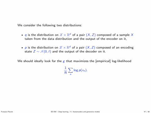
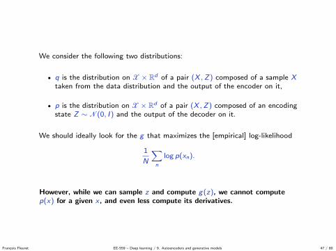
We consider the following two distributions:
• q is the distribution on X × Rd of a pair (X ,Z) composed of a sample Xtaken from the data distribution and the output of the encoder on it,
• p is the distribution on X × Rd of a pair (X ,Z) composed of an encodingstate Z ∼ N(0, I ) and the output of the decoder on it.
We should ideally look for the g that maximizes the [empirical] log-likelihood
1
N
∑n
log p(xn).
However, while we can sample z and compute g(z), we cannot computep(x) for a given x, and even less compute its derivatives.
Francois Fleuret EE-559 – Deep learning / 9. Autoencoders and generative models 47 / 80

The Variational Autoencoder proposed by Kingma and Welling (2013) relieson a tractable approximation of this log-likelihood.
Their framework considers a stochastic encoder f , and decoder g , whoseoutputs depend on their inputs as usual but with some remaining randomness.
Francois Fleuret EE-559 – Deep learning / 9. Autoencoders and generative models 48 / 80

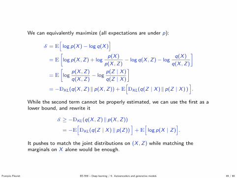
We can equivalently maximize (all expectations are under p):
S = E[
log p(X )− log q(X )]
= E
[log p(X ,Z) + log
p(X )
p(X ,Z)− log q(X ,Z)− log
q(X )
q(X ,Z)
]= E
[log
p(X ,Z)
q(X ,Z)− log
p(Z | X )
q(Z | X )
]= −DKL(q(X ,Z) ‖ p(X ,Z)) + E
[DKL(q(Z | X ) ‖ p(Z | X ) )
].
While the second term cannot be properly estimated, we can use the first as alower bound, and rewrite it
S ≥ −DKL(q(X ,Z) ‖ p(X ,Z))
= −E[DKL(q(Z | X ) ‖ p(Z))
]+ E
[log p(X | Z)
].
It pushes to match the joint distributions on (X ,Z) while matching themarginals on X alone would be enough.
Francois Fleuret EE-559 – Deep learning / 9. Autoencoders and generative models 49 / 80

Kingma and Welling use Gaussians with diagonal covariance for both q(Z | X )and p(X | Z).
So in practice the encoder maps a data point from the signal space Rc to [theparameters of] a Gaussian in the latent space Rd
f : Rc → R2d
x 7→(µf1, . . . , µ
fd , σ
f1 , . . . , σ
fd
),
and the decoder maps a latent value from Rd to [the parameters of] a Gaussianin the signal space Rc
g : Rd → R2c
z 7→(µg1 , . . . , µ
gc , σ
g1 , . . . , σ
gc
).
Francois Fleuret EE-559 – Deep learning / 9. Autoencoders and generative models 50 / 80
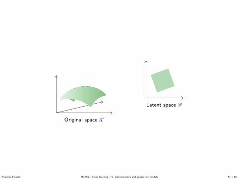
Original space X
Latent space F
f
g
Francois Fleuret EE-559 – Deep learning / 9. Autoencoders and generative models 51 / 80

Original space X
Latent space F
f
g
Francois Fleuret EE-559 – Deep learning / 9. Autoencoders and generative models 51 / 80

Original space X
Latent space F
f
g
Francois Fleuret EE-559 – Deep learning / 9. Autoencoders and generative models 51 / 80

Original space X
Latent space F
f
g
Francois Fleuret EE-559 – Deep learning / 9. Autoencoders and generative models 51 / 80

Original space X
Latent space F
f
g
Francois Fleuret EE-559 – Deep learning / 9. Autoencoders and generative models 51 / 80

We have to minimize
L = E[DKL (q(Z | X ) ‖ p(Z))
]− E
[log p(X | Z)
].
Since q(Z | X ) and p(Z) are Gaussian, we have
DKL (q(Z | X = x) ‖ p(Z)) =1
2
∑d
(1 + 2 log σf
d (x)−(µfd (x)
)2−(σfd (x)
)2).
And with
znl ∼ N(µf (xn), σf (xn)
), n = 1, . . . ,N, l = 1, . . . , L,
we have
−E[
log p(X | Z)]'
1
2
N∑n=1
L∑l=1
∑c
(xn,d − µgc (znl )
)2
2(σgc (znl )
)2
Kingma and Welling point out that using L = 1 is enough.
Francois Fleuret EE-559 – Deep learning / 9. Autoencoders and generative models 52 / 80

For MNIST, we keep our convolutional structure, but the encoder now maps totwice the number of dimensions, which corresponds to the µf s and σf s, and weuse a fixed variance for the decoder.
We use Adam for training and the loss estimate for the standard autoencoder
output = model(input)
loss = mse_loss(output , input)
becomes
param = model.encode(input)
mu, logvar = param.split(param.size (1)//2, 1)
logvar = logvar + math.log (0.01)
std = logvar.mul (0.5).exp()
kl = - 0.5 * (1 + logvar - mu.pow (2) - logvar.exp())
kl = kl.mean()
u = Variable(mu.data.new(mu.size()).normal_ ())
z = u * std + mu
output = model.decode(z)
loss = mse_loss(output , input) + 0.5 * kl
During inference we do not sample, and instead use µf and µg as prediction.
Francois Fleuret EE-559 – Deep learning / 9. Autoencoders and generative models 53 / 80

Original
Autoencoder reconstruction (d = 32)
Variational Autoencoder reconstruction (d = 32)
Francois Fleuret EE-559 – Deep learning / 9. Autoencoders and generative models 54 / 80

Autoencoder sampling (d = 32)
Variational Autoencoder sampling (d = 32)
Francois Fleuret EE-559 – Deep learning / 9. Autoencoders and generative models 55 / 80

Non-Volume Preserving network
Francois Fleuret EE-559 – Deep learning / 9. Autoencoders and generative models 56 / 80
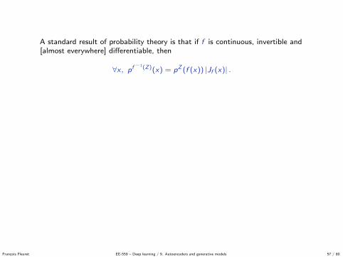
A standard result of probability theory is that if f is continuous, invertible and[almost everywhere] differentiable, then
∀x , pf−1(Z)(x) = pZ (f (x)) |Jf (x)| .
f
1
3
pZ
1 5pf−1(Z)
Francois Fleuret EE-559 – Deep learning / 9. Autoencoders and generative models 57 / 80

A standard result of probability theory is that if f is continuous, invertible and[almost everywhere] differentiable, then
∀x , pf−1(Z)(x) = pZ (f (x)) |Jf (x)| .
f
1
3
pZ
1 5pf−1(Z)
Francois Fleuret EE-559 – Deep learning / 9. Autoencoders and generative models 57 / 80

A standard result of probability theory is that if f is continuous, invertible and[almost everywhere] differentiable, then
∀x , pf−1(Z)(x) = pZ (f (x)) |Jf (x)| .
f
1
3
pZ
1 5pf−1(Z)
Francois Fleuret EE-559 – Deep learning / 9. Autoencoders and generative models 57 / 80

A standard result of probability theory is that if f is continuous, invertible and[almost everywhere] differentiable, then
∀x , pf−1(Z)(x) = pZ (f (x)) |Jf (x)| .
f
1
3
pZ
1 5pf−1(Z)
Francois Fleuret EE-559 – Deep learning / 9. Autoencoders and generative models 57 / 80

From this equality, if f is a parametric function such that we can compute [anddifferentiate]
pZ (f (x))
and|Jf (x)|
then, we can make the distribution of f −1(Z) fits the data by optimizing∑n
log pf−1(Z)(xn)
=∑n
log(pZ (f (xn)) |Jf (xn)|
).
If we are able to do so, then we can synthesize a new X by samplingZ ∼ N(0, 1) and computing f −1(Z).
Francois Fleuret EE-559 – Deep learning / 9. Autoencoders and generative models 58 / 80

From this equality, if f is a parametric function such that we can compute [anddifferentiate]
pZ (f (x))
and|Jf (x)|
then, we can make the distribution of f −1(Z) fits the data by optimizing∑n
log pf−1(Z)(xn) =
∑n
log(pZ (f (xn)) |Jf (xn)|
).
If we are able to do so, then we can synthesize a new X by samplingZ ∼ N(0, 1) and computing f −1(Z).
Francois Fleuret EE-559 – Deep learning / 9. Autoencoders and generative models 58 / 80

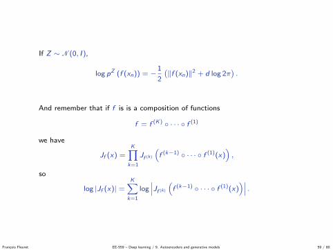
If Z ∼ N(0, I ),
log pZ (f (xn)) = −1
2
(‖f (xn)‖2 + d log 2π
).
And remember that if f is is a composition of functions
f = f (K) ◦ · · · ◦ f (1)
we have
Jf (x) =K∏
k=1
Jf (k)
(f (k−1) ◦ · · · ◦ f (1)(x)
),
so
log |Jf (x)| =K∑
k=1
log∣∣∣Jf (k)
(f (k−1) ◦ · · · ◦ f (1)(x)
)∣∣∣ .
Francois Fleuret EE-559 – Deep learning / 9. Autoencoders and generative models 59 / 80

If f (k) are standard layers we cannot compute f −1(z), and computing |Jf (x)| isintractable.
Dinh et al. (2014) introduced the coupling layers to address both issues.
The resulting Non-Volume Preserving network (NVP) is an example of aNormalizing flow (Rezende and Mohamed, 2015).
Francois Fleuret EE-559 – Deep learning / 9. Autoencoders and generative models 60 / 80

We use here the formalism from Dinh et al. (2016).
Given a dimension d , a Boolean vector b ∈ {0, 1}d and two mappings
s :Rd → Rd
t :Rd → Rd ,
we define a [fully connected] coupling layer as the transformation
c : Rd → Rd
x 7→ b � x + (1− b)�(x � exp(s(b � x)) + t(b � x)
)where exp is component-wise, and � is the Hadamard component-wise product.
Francois Fleuret EE-559 – Deep learning / 9. Autoencoders and generative models 61 / 80
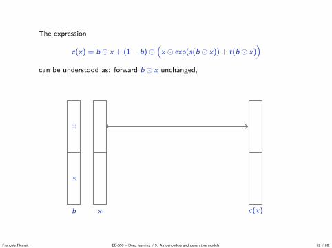
The expression
c(x) = b � x + (1− b)�(x � exp(s(b � x)) + t(b � x)
)can be understood as: forward b � x unchanged,
and apply to (1− b)� x aninvertible transformation parametrized by b � x .
(0)
(1)
xb c(x)
s exp t
� +
Francois Fleuret EE-559 – Deep learning / 9. Autoencoders and generative models 62 / 80

The expression
c(x) = b � x + (1− b)�(x � exp(s(b � x)) + t(b � x)
)can be understood as: forward b � x unchanged, and apply to (1− b)� x aninvertible transformation parametrized by b � x .
(0)
(1)
xb c(x)
s exp t
� +
Francois Fleuret EE-559 – Deep learning / 9. Autoencoders and generative models 62 / 80

The consequence is that c is invertible, and if y = c(x)
x = b � y + (1− b)�(y − t(b � y)
)� exp(−s(b � y)).
(0)
(1)
c(x)b x
−s exp−t
+ �
Francois Fleuret EE-559 – Deep learning / 9. Autoencoders and generative models 63 / 80

The consequence is that c is invertible, and if y = c(x)
x = b � y + (1− b)�(y − t(b � y)
)� exp(−s(b � y)).
(0)
(1)
c(x)b x
−s exp−t
+ �
Francois Fleuret EE-559 – Deep learning / 9. Autoencoders and generative models 63 / 80

The second property of this mapping is the simplicity of its Jacobiandeterminant.
Since
ci (x) = bi � xi + (1− bi )�(xi � exp(si (b � x)) + ti (b � x)
)we have, ∀i , j , x ,
bi = 1 ⇒ ci (x) = xi
⇒∂ci
∂xj= 1{i=j}
and
bi = 0 ⇒ ci (x) = xi exp(si (b � x)) + ti (b � x)
⇒∂ci
∂xj=(
1{i=j} + xi∂si (b � x)
∂xj︸ ︷︷ ︸0 if bj=0
)exp(si (b � x)) +
∂ti (b � x)
∂xj︸ ︷︷ ︸0 if bj=0
⇒∂ci
∂xj= 1{i=j} exp(si (b � x)) + bj
(...).
Hence ∂ci∂xj
can be non-zero only if i = j , or (1− bi )bj = 1.
Francois Fleuret EE-559 – Deep learning / 9. Autoencoders and generative models 64 / 80

The second property of this mapping is the simplicity of its Jacobiandeterminant. Since
ci (x) = bi � xi + (1− bi )�(xi � exp(si (b � x)) + ti (b � x)
)we have, ∀i , j , x ,
bi = 1 ⇒ ci (x) = xi
⇒∂ci
∂xj= 1{i=j}
and
bi = 0 ⇒ ci (x) = xi exp(si (b � x)) + ti (b � x)
⇒∂ci
∂xj=(
1{i=j} + xi∂si (b � x)
∂xj︸ ︷︷ ︸0 if bj=0
)exp(si (b � x)) +
∂ti (b � x)
∂xj︸ ︷︷ ︸0 if bj=0
⇒∂ci
∂xj= 1{i=j} exp(si (b � x)) + bj
(...).
Hence ∂ci∂xj
can be non-zero only if i = j , or (1− bi )bj = 1.
Francois Fleuret EE-559 – Deep learning / 9. Autoencoders and generative models 64 / 80
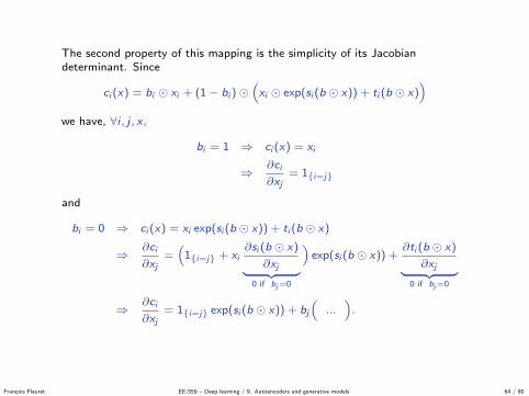
The second property of this mapping is the simplicity of its Jacobiandeterminant. Since
ci (x) = bi � xi + (1− bi )�(xi � exp(si (b � x)) + ti (b � x)
)we have, ∀i , j , x ,
bi = 1 ⇒ ci (x) = xi
⇒∂ci
∂xj= 1{i=j}
and
bi = 0 ⇒ ci (x) = xi exp(si (b � x)) + ti (b � x)
⇒∂ci
∂xj=(
1{i=j} + xi∂si (b � x)
∂xj︸ ︷︷ ︸0 if bj=0
)exp(si (b � x)) +
∂ti (b � x)
∂xj︸ ︷︷ ︸0 if bj=0
⇒∂ci
∂xj= 1{i=j} exp(si (b � x)) + bj
(...).
Hence ∂ci∂xj
can be non-zero only if i = j , or (1− bi )bj = 1.
Francois Fleuret EE-559 – Deep learning / 9. Autoencoders and generative models 64 / 80
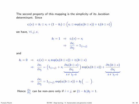
The second property of this mapping is the simplicity of its Jacobiandeterminant. Since
ci (x) = bi � xi + (1− bi )�(xi � exp(si (b � x)) + ti (b � x)
)we have, ∀i , j , x ,
bi = 1 ⇒ ci (x) = xi
⇒∂ci
∂xj= 1{i=j}
and
bi = 0 ⇒ ci (x) = xi exp(si (b � x)) + ti (b � x)
⇒∂ci
∂xj=(
1{i=j} + xi∂si (b � x)
∂xj︸ ︷︷ ︸0 if bj=0
)exp(si (b � x)) +
∂ti (b � x)
∂xj︸ ︷︷ ︸0 if bj=0
⇒∂ci
∂xj= 1{i=j} exp(si (b � x)) + bj
(...).
Hence ∂ci∂xj
can be non-zero only if i = j , or (1− bi )bj = 1.
Francois Fleuret EE-559 – Deep learning / 9. Autoencoders and generative models 64 / 80

If we re-order both the rows and columns of the Jacobian to put first thenon-zeros entries of b, and then the zeros, it becomes lower triangular
Jc (x) =
1
. . . (0)1
exp(sk (x � b))
(6= 0). . .
exp(sk′ (x � b))
its determinant remains unchanged, and we have
log |Jf (k) (x)| =∑i :bi=0
si (x � b)
=∑i
((1− b)� s (x � b))i .
Francois Fleuret EE-559 – Deep learning / 9. Autoencoders and generative models 65 / 80

dim = 6
x = Variable(Tensor(1, dim).normal_ (), requires_grad = True)
b = Variable(Tensor(1, dim).zero_ ())
b.data.narrow(1, 0, dim //2).fill_ (1.0)
s = nn.Sequential(nn.Linear(dim , dim), nn.Tanh())
t = nn.Sequential(nn.Linear(dim , dim), nn.Tanh())
c = b * x + (1 - b) * (x * s(b * x).exp() + t(b * x))
j = torch.cat([torch.autograd.grad(c_k , x, retain_graph=True)[0] for c_k in c[0]])
print(j)
prints
1.0000 0.0000 0.0000 0.0000 0.0000 0.0000
0.0000 1.0000 0.0000 0.0000 0.0000 0.0000
0.0000 0.0000 1.0000 0.0000 0.0000 0.0000
-0.8182 0.5622 -0.4035 1.4700 0.0000 0.0000
0.2610 0.1475 0.1689 0.0000 1.1358 0.0000
-0.2910 0.0287 0.0194 0.0000 0.0000 0.8508
[torch.FloatTensor of size 6x6]
Francois Fleuret EE-559 – Deep learning / 9. Autoencoders and generative models 66 / 80
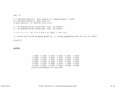

To recap, with f (k), k = 1, . . . ,K coupling layers,
f = f (K) ◦ · · · ◦ f (1),
and x(0)n = xn and x
(k)n = f (k)
(x
(k−1)n
),
we train by maximizing
L(f ) =∑n
(−
1
2
(∥∥∥x(K)n
∥∥∥2+ d log 2π
)+
K∑k=1
log∣∣∣Jf (k)
(x
(k−1)n
)∣∣∣) ,with
log |Jf (k) (x)| =∑i
((1− b(k)
)� s(k)
(x � b(k)
))i.
And to sample we just need to generate Z ∼ N(0, I ) and compute f −1(Z).
Francois Fleuret EE-559 – Deep learning / 9. Autoencoders and generative models 67 / 80

To recap, with f (k), k = 1, . . . ,K coupling layers,
f = f (K) ◦ · · · ◦ f (1),
and x(0)n = xn and x
(k)n = f (k)
(x
(k−1)n
), we train by maximizing
L(f ) =∑n
(−
1
2
(∥∥∥x(K)n
∥∥∥2+ d log 2π
)+
K∑k=1
log∣∣∣Jf (k)
(x
(k−1)n
)∣∣∣) ,with
log |Jf (k) (x)| =∑i
((1− b(k)
)� s(k)
(x � b(k)
))i.
And to sample we just need to generate Z ∼ N(0, I ) and compute f −1(Z).
Francois Fleuret EE-559 – Deep learning / 9. Autoencoders and generative models 67 / 80
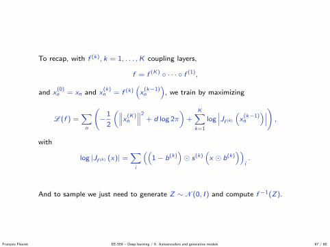
To recap, with f (k), k = 1, . . . ,K coupling layers,
f = f (K) ◦ · · · ◦ f (1),
and x(0)n = xn and x
(k)n = f (k)
(x
(k−1)n
), we train by maximizing
L(f ) =∑n
(−
1
2
(∥∥∥x(K)n
∥∥∥2+ d log 2π
)+
K∑k=1
log∣∣∣Jf (k)
(x
(k−1)n
)∣∣∣) ,with
log |Jf (k) (x)| =∑i
((1− b(k)
)� s(k)
(x � b(k)
))i.
And to sample we just need to generate Z ∼ N(0, I ) and compute f −1(Z).
Francois Fleuret EE-559 – Deep learning / 9. Autoencoders and generative models 67 / 80

A coupling layer can be implemented with
class NVPCouplingLayer(Module):
def __init__(self , map_s , map_t , b):
super(NVPCouplingLayer , self).__init__ ()
self.map_s = map_s
self.map_t = map_t
self.b = Variable(b.clone().unsqueeze (0), requires_grad = False)
def forward(self , x_and_logdetjac):
x, logdetjac = x_and_logdetjac
s, t = self.map_s(self.b * x), self.map_t(self.b * x)
logdetjac += ((1 - self.b) * s).sum(1)
y = self.b * x + (1 - self.b) * (torch.exp(s) * x + t)
return (y, logdetjac)
def invert(self , y):
s, t = self.map_s(self.b * y), self.map_t(self.b * y)
return self.b * y + (1 - self.b) * (torch.exp(-s) * (y - t))
The forward here computes both the image of x and the update on theaccumulated determinant of the Jacobian, i.e.
(x , u) 7→ (f (x), u + |Jf (x)|) .
Francois Fleuret EE-559 – Deep learning / 9. Autoencoders and generative models 68 / 80

We can then define a complete network with one-hidden layer tanh MLPs forthe s and t mappings
class NVPNet(Module):
def __init__(self , dim , hdim , depth):
super(NVPNet , self).__init__ ()
b = Tensor(dim)
self.layers = nn.ModuleList ()
for d in range(depth):
if d%2 == 0:
# Tag half the dimensions
i = torch.randperm(b.numel()).narrow(0, 0, b.numel() // 2)
b.zero_()[i] = 1
else:
b = 1 - b
map_s = nn.Sequential(nn.Linear(dim , hdim), nn.Tanh(), nn.Linear(hdim , dim))
map_t = nn.Sequential(nn.Linear(dim , hdim), nn.Tanh(), nn.Linear(hdim , dim))
self.layers.append(NVPCouplingLayer(map_s , map_t , b))
def forward(self , x):
for m in self.layers: x = m(x)
return x
def invert(self , y):
for m in reversed(self.layers): y = m.invert(y)
return y
Francois Fleuret EE-559 – Deep learning / 9. Autoencoders and generative models 69 / 80

And the log-proba of individual samples of a batch
def LogProba(x_and_logdetjac):
(x, logdetjac) = x_and_logdetjac
log_p = logdetjac - 0.5 * x.pow (2).add(math.log(2 * math.pi)).sum (1)
return log_p
Francois Fleuret EE-559 – Deep learning / 9. Autoencoders and generative models 70 / 80

Training is achieved by maximizing the mean log-proba
batch_size = 100
model = NVPNet(dim = 2, hidden_dim = 2, depth = 4)
optimizer = optim.Adam(model.parameters (), lr = 1e-2)
for e in range(args.nb_epochs):
for b in range(0, nb_train_samples , batch_size):
output = model(( input.narrow(0, b, batch_size), 0))
loss = - LogProba(output).mean()
model.zero_grad ()
loss.backward ()
optimizer.step()
Finally, we can sample according to pf−1(Z) with
z = Variable(Tensor(nb_train_samples , dim).normal_ ())
x = model.invert(z).data
Francois Fleuret EE-559 – Deep learning / 9. Autoencoders and generative models 71 / 80

-4
-3
-2
-1
0
1
2
3
4
-6 -4 -2 0 2 4 6
RealSynth
Francois Fleuret EE-559 – Deep learning / 9. Autoencoders and generative models 72 / 80
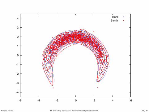
-4
-3
-2
-1
0
1
2
3
4
-6 -4 -2 0 2 4 6
RealSynth
Francois Fleuret EE-559 – Deep learning / 9. Autoencoders and generative models 72 / 80

-4
-3
-2
-1
0
1
2
3
4
-6 -4 -2 0 2 4 6
RealSynth
Francois Fleuret EE-559 – Deep learning / 9. Autoencoders and generative models 72 / 80

-4
-3
-2
-1
0
1
2
3
4
-6 -4 -2 0 2 4 6
RealSynth
Francois Fleuret EE-559 – Deep learning / 9. Autoencoders and generative models 72 / 80

-4
-3
-2
-1
0
1
2
3
4
-6 -4 -2 0 2 4 6
RealSynth
Francois Fleuret EE-559 – Deep learning / 9. Autoencoders and generative models 72 / 80

Dinh et al. (2016) apply this approach to convolutional layers by using bsconsistent with the activation map structure, and reducing the map size whileincreasing the number of channels.
Published as a conference paper at ICLR 2017
4 8
732
1 2
3 4
5 6
7 861 5
Figure 3: Masking schemes for affine coupling layers. On the left, a spatial checkerboard patternmask. On the right, a channel-wise masking. The squeezing operation reduces the 4× 4× 1 tensor(on the left) into a 2× 2× 4 tensor (on the right). Before the squeezing operation, a checkerboardpattern is used for coupling layers while a channel-wise masking pattern is used afterward.
(see Figure 2(b)),{y1:d = x1:dyd+1:D = xd+1:D � exp
(s(x1:d)
)+ t(x1:d)
(7)
⇔{x1:d = y1:dxd+1:D =
(yd+1:D − t(y1:d)
)� exp
(− s(y1:d)
),
(8)
meaning that sampling is as efficient as inference for this model. Note again that computing theinverse of the coupling layer does not require computing the inverse of s or t, so these functions canbe arbitrarily complex and difficult to invert.
3.4 Masked convolution
Partitioning can be implemented using a binary mask b, and using the functional form for y,
y = b� x+ (1− b)�(x� exp
(s(b� x)
)+ t(b� x)
). (9)
We use two partitionings that exploit the local correlation structure of images: spatial checkerboardpatterns, and channel-wise masking (see Figure 3). The spatial checkerboard pattern mask has value1 where the sum of spatial coordinates is odd, and 0 otherwise. The channel-wise mask b is 1 for thefirst half of the channel dimensions and 0 for the second half. For the models presented here, boths(·) and t(·) are rectified convolutional networks.
3.5 Combining coupling layers
Although coupling layers can be powerful, their forward transformation leaves some componentsunchanged. This difficulty can be overcome by composing coupling layers in an alternating pattern,such that the components that are left unchanged in one coupling layer are updated in the next (seeFigure 4(a)).
The Jacobian determinant of the resulting function remains tractable, relying on the fact that
∂(fb ◦ fa)∂xTa
(xa) =∂fa
∂xTa(xa) ·
∂fb
∂xTb
(xb = fa(xa)
)(10)
det(A ·B) = det(A) det(B). (11)
Similarly, its inverse can be computed easily as
(fb ◦ fa)−1 = f−1a ◦ f−1b . (12)
5
(Dinh et al., 2016)
Francois Fleuret EE-559 – Deep learning / 9. Autoencoders and generative models 73 / 80

They combine these layers by alternating masks, and branching out half of thechannels at certain points to forward them unchanged.
Published as a conference paper at ICLR 2017
=
+x
+x
=
=
+x
(a) In this alternating pattern, units which remain identical in onetransformation are modified in the next.
z1 z2
x1 x2 x3 x4
z3
z1 z2 z3 z4
(1) (1)
(2)
f(1)
f(2)
f(3)
h4
h4h3
(b) Factoring out variables.At each step, half the vari-ables are directly modeled asGaussians, while the otherhalf undergo further transfor-mation.
Figure 4: Composition schemes for affine coupling layers.
3.6 Multi-scale architecture
We implement a multi-scale architecture using a squeezing operation: for each channel, it divides theimage into subsquares of shape 2× 2× c, then reshapes them into subsquares of shape 1× 1× 4c.The squeezing operation transforms an s × s × c tensor into an s
2 × s2 × 4c tensor (see Figure 3),
effectively trading spatial size for number of channels.
At each scale, we combine several operations into a sequence: we first apply three coupling layerswith alternating checkerboard masks, then perform a squeezing operation, and finally apply threemore coupling layers with alternating channel-wise masking. The channel-wise masking is chosen sothat the resulting partitioning is not redundant with the previous checkerboard masking (see Figure3). For the final scale, we only apply four coupling layers with alternating checkerboard masks.
Propagating a D dimensional vector through all the coupling layers would be cumbersome, in termsof computational and memory cost, and in terms of the number of parameters that would need to betrained. For this reason we follow the design choice of [57] and factor out half of the dimensions atregular intervals (see Equation 14). We can define this operation recursively (see Figure 4(b)),
h(0) = x (13)
(z(i+1), h(i+1)) = f (i+1)(h(i)) (14)
z(L) = f (L)(h(L−1)) (15)
z = (z(1), . . . , z(L)). (16)
In our experiments, we use this operation for i < L. The sequence of coupling-squeezing-couplingoperations described above is performed per layer when computing f (i) (Equation 14). At eachlayer, as the spatial resolution is reduced, the number of hidden layer features in s and t is doubled.All variables which have been factored out at different scales are concatenated to obtain the finaltransformed output (Equation 16).
As a consequence, the model must Gaussianize units which are factored out at a finer scale (in anearlier layer) before those which are factored out at a coarser scale (in a later layer). This results in thedefinition of intermediary levels of representation [53, 49] corresponding to more local, fine-grainedfeatures as shown in Appendix D.
Moreover, Gaussianizing and factoring out units in earlier layers has the practical benefit of distribut-ing the loss function throughout the network, following the philosophy similar to guiding intermediatelayers using intermediate classifiers [40]. It also reduces significantly the amount of computation andmemory used by the model, allowing us to train larger models.
6
(Dinh et al., 2016)
Francois Fleuret EE-559 – Deep learning / 9. Autoencoders and generative models 74 / 80

The structure for generating images consists of
• ×2 stages• ×3 checkerboard coupling layers,• a squeezing layer,• ×3 channel coupling layers,• a factor-out layer.
• ×1 stage• ×4 checkerboard coupling layers• a factor-out layer.
The s and t mappings get more complex in the later layers.
Francois Fleuret EE-559 – Deep learning / 9. Autoencoders and generative models 75 / 80

A Samples
Figure 7: Samples from a model trained on Imagenet (64× 64).
13
(Dinh et al., 2016)
Francois Fleuret EE-559 – Deep learning / 9. Autoencoders and generative models 76 / 80

Figure 8: Samples from a model trained on CelebA.
14
(Dinh et al., 2016)
Francois Fleuret EE-559 – Deep learning / 9. Autoencoders and generative models 77 / 80

Figure 9: Samples from a model trained on LSUN (bedroom category).
15
(Dinh et al., 2016)
Francois Fleuret EE-559 – Deep learning / 9. Autoencoders and generative models 78 / 80
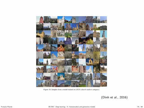
Figure 10: Samples from a model trained on LSUN (church outdoor category).
16
(Dinh et al., 2016)
Francois Fleuret EE-559 – Deep learning / 9. Autoencoders and generative models 79 / 80

Figure 6: Manifold generated from four examples in the dataset. Clockwise from top left: CelebA,Imagenet (64× 64), LSUN (tower), LSUN (bedroom).
over sample quality in a limited capacity setting. As a result, our model outputs sometimes highlyimprobable samples as we can notice especially on CelebA. As opposed to variational autoencoders,the samples generated from our model look not only globally coherent but also sharp. Our hypothesisis that as opposed to these models, real NVP does not rely on fixed form reconstruction cost like an L2
norm which tends to reward capturing low frequency components more heavily than high frequencycomponents. Unlike autoregressive models, sampling from our model is done very efficiently as it isparallelized over input dimensions. On Imagenet and LSUN, our model seems to have captured wellthe notion of background/foreground and lighting interactions such as luminosity and consistent lightsource direction for reflectance and shadows.
We also illustrate the smooth semantically consistent meaning of our latent variables. In the latentspace, we define a manifold based on four validation examples z(1), z(2), z(3), z(4), and parametrizedby two parameters φ and φ′ by,
z = cos(φ)(cos(φ′)z(1) + sin(φ′)z(2)
)+ sin(φ)
(cos(φ′)z(3) + sin(φ′)z(4)
). (19)
We project the resulting manifold back into the data space by computing g(z). Results are shownFigure 6. We observe that the model seems to have organized the latent space with a notion of meaningthat goes well beyond pixel space interpolation. More visualization are shown in the Appendix.
5 Discussion and conclusion
In this paper, we have defined a class of invertible functions with tractable Jacobian determinant,enabling exact and tractable log-likelihood evaluation, inference, and sampling. We have shown thatthis class of generative model achieves competitive performances, both in terms of sample qualityand log-likelihood. Many avenues exist to further improve the functional form of the transformations,for instance by exploiting the latest advances in dilated convolutions [69] and residual networksarchitectures [60].
This paper presented a technique bridging the gap between auto-regressive models, variationalautoencoders, and generative adversarial networks. Like auto-regressive models, it allows tractableand exact log-likelihood evaluation for training. It allows however a much more flexible functionalform, similar to that in the generative model of variational autoencoders. This allows for fastand exact sampling from the model distribution. Like GANs, and unlike variational autoencoders,our technique does not require the use of a fixed form reconstruction cost, and instead defines acost in terms of higher level features, generating sharper images. Finally, unlike both variationalautoencoders and GANs, our technique is able to learn a semantically meaningful latent space whichis as high dimensional as the input space. This may make the algorithm particularly well suited tosemi-supervised learning tasks, as we hope to explore in future work.
9
(Dinh et al., 2016)
Francois Fleuret EE-559 – Deep learning / 9. Autoencoders and generative models 80 / 80

The end
References
L. Dinh, D. Krueger, and Y. Bengio. NICE: non-linear independent components estimation.CoRR, abs/1410.8516, 2014.
L. Dinh, J. Sohl-Dickstein, and S. Bengio. Density estimation using real NVP. CoRR,abs/1605.08803, 2016.
D. P. Kingma and M. Welling. Auto-encoding variational bayes. CoRR, abs/1312.6114,2013.
D. Rezende and S. Mohamed. Variational inference with normalizing flows. CoRR,abs/1505.05770, 2015.
P. Vincent, H. Larochelle, I. Lajoie, Y. Bengio, and P.-A. Manzagol. Stacked denoisingautoencoders: Learning useful representations in a deep network with a local denoisingcriterion. Journal of Machine Learning Research (JMLR), 11:3371–3408, 2010.