Extracting and Composing Robust Features with

Denoising Autoencoders

Pascal Vincent, Hugo Larochelle, Yoshua Bengio, Pierre-Antoine ManzagolDept. IRO, Universite de Montreal

C.P. 6128, Montreal, Qc, H3C 3J7, Canadahttp://www.iro.umontreal.ca/∼lisa

Technical Report 1316, February 2008

Abstract

Previous work has shown that the difficulties in learning deep genera-tive or discriminative models can be overcome by an initial unsupervisedlearning step that maps inputs to useful intermediate representations. Weintroduce and motivate a new training principle for unsupervised learningof a representation based on the idea of making the learned representa-tions robust to partial corruption of the input pattern. This approach canbe used to train autoencoders, and these denoising autoencoders can bestacked to initialize deep architectures. The algorithm can be motivatedfrom a manifold learning and information theoretic perspective or from agenerative model perspective. Comparative experiments clearly show thesurprising advantage of corrupting the input of autoencoders on a patternclassification benchmark suite.

1 Introduction

Recent theoretical studies indicate that deep architectures (Bengio & Le Cun,2007; Bengio, 2007) may be needed to efficiently model complex distributionsand achieve better generalization performance on challenging recognition tasks.The belief that additional levels of functional composition will yield increasedrepresentational and modeling power is not new (McClelland et al., 1986; Hin-ton, 1989; Utgoff & Stracuzzi, 2002). However, in practice, learning in deeparchitectures has proven to be difficult. One needs only to ponder the diffi-cult problem of inference in deep directed graphical models, due to “explainingaway”. Also looking back at the history of multi-layer neural networks, theirdifficult optimization (Bengio et al., 2007; Bengio, 2007) has long preventedreaping the expected benefits of going beyond one or two hidden layers. How-ever this situation has recently changed with the successful approach of (Hintonet al., 2006; Hinton & Salakhutdinov, 2006; Bengio et al., 2007; Ranzato et al.,2007; Lee et al., 2008) for training Deep Belief Networks and stacked autoen-coders.

1

One key ingredient to this success appears to be the use of an unsupervisedtraining criterion to perform a layer-by-layer initialization: each layer is at firsttrained to produce a higher level (hidden) representation of the observed pat-terns, based on the representation it receives as input from the layer below, byoptimizing a local unsupervised criterion. Each level produces a representationof the input pattern that is more abstract than the previous level’s, because itis obtained by composing more operations. This initialization yields a startingpoint, from which a global fine-tuning of the model’s parameters is then per-formed using another training criterion appropriate for the task at hand. Thistechnique has been shown empirically to avoid getting stuck in the kind of poorsolutions one typically reaches with random initializations. While unsupervisedlearning of a mapping that produces “good” intermediate representations ofthe input pattern seems to be key, little is understood regarding what consti-tutes “good” representations for initializing deep architectures, or what explicitcriteria may guide learning such representations. We know of only a few algo-rithms that seem to work well for this purpose: Restricted Boltzmann Machines(RBMs) trained with contrastive divergence on one hand, and various types ofautoencoders on the other.

The present research begins with the question of what explicit criteria a goodintermediate representation should satisfy. Obviously, it should at a minimumretain a certain amount of “information” about its input, while at the same timebeing constrained to a given form (e.g. a real-valued vector of a given size in thecase of an autoencoder). A supplemental criterion that has been proposed forsuch models is sparsity of the representation (Ranzato et al., 2008; Lee et al.,2008). Here we hypothesize and investigate an additional specific criterion:robustness to partial destruction of the input, i.e., partially destructedinputs should yield almost the same representation. It is motivated by thefollowing informal reasoning: a good representation is expected to capture stablestructures in the form of dependencies and regularities characteristic of the(unknown) distribution of its observed input. For high dimensional redundantinput (such as images) at least, such structures are likely to depend on evidencegathered from a combination of many input dimensions. They should thus berecoverable from partial observation only. A hallmark of this is our humanability to recognize partially occluded or corrupted images. Further evidence isour ability to form a high level concept associated to multiple modalities (suchas image and sound) and recall it even when some of the modalities are missing.

To validate our hypothesis and assess its usefulness as one of the guidingprinciples in learning deep architectures, we propose a modification to the au-toencoder framework to explicitly integrate robustness to partially destroyedinputs. Section 2 describes the algorithm in details. Section 3 discusses linkswith other approaches in the literature. Section 4 is devoted to a closer inspec-tion of the model from different theoretical standpoints. In section 5 we verifyempirically if the algorithm leads to a difference in performance. Section 6concludes the study.

2

2 Description of the Algorithm

2.1 Notation and Setup

Let X and Y be two random variables with joint probability density p(X, Y ),with marginal distributions p(X) and p(Y ). Throughout the text, we willuse the following notation: Expectation: EEp(X)[f(X)] =

∫p(x)f(x)dx. En-

tropy: IH(X) = IH(p) = EEp(X)[− log p(X)]. Conditional entropy: IH(X|Y ) =EEp(X,Y )[− log p(X|Y )]. Kullback-Leibler divergence: IDKL(p‖q) = EEp(X)[log p(X)

q(X) ].Cross-entropy: IH(p‖q) = EEp(X)[− log q(X)] = IH(p) + IDKL(p‖q). Mutual infor-mation: I(X;Y ) = IH(X) − IH(X|Y ). Sigmoid: s(x) = 1

1+e−x and s(x) =(s(x1), . . . , s(xd))T . Bernoulli distribution with mean µ: Bµ(x). and by exten-sion Bµ(x) = (Bµ1(x1), . . . ,Bµd

(xd)).The setup we consider is the typical supervised learning setup with a training

set of n (input, target) pairs Dn = {(x(1), t(1)) . . . , (x(n), t(n))}, that we supposeto be an i.i.d. sample from an unknown distribution q(X, T ) with correspondingmarginals q(X) and q(T ).

2.2 The Basic Autoencoder

We begin by recalling the traditional autoencoder model such as the one usedin (Bengio et al., 2007) to build deep networks. An autoencoder takes an inputvector x ∈ [0, 1]d, and first maps it to a hidden representation y ∈ [0, 1]d

′

through a deterministic mapping y = fθ(x) = s(Wx + b), parameterized byθ = {W,b}. W is a d′ × d weight matrix and b is a bias vector. The resultinglatent representation y is then mapped back to a “reconstructed” vector z ∈[0, 1]d in input space z = gθ′(y) = s(W′y +b′) with θ′ = {W′,b′}. The weightmatrix W′ of the reverse mapping may optionally be constrained by W′ = WT ,in which case the autoencoder is said to have tied weights. Each training x(i) isthus mapped to a corresponding y(i) and a reconstruction z(i). The parametersof this model are optimized to minimize the average reconstruction error:

θ?, θ′? = arg minθ,θ′

1n

n∑i=1

L(x(i), z(i)

)= arg min

θ,θ′

1n

n∑i=1

L(x(i), gθ′(fθ(x(i)))

)(1)

where L is a loss function such as the traditional squared error L(x, z) = ‖x−z‖2.An alternative loss, suggested by the interpretation of x and z as either bitvectors or vectors of bit probabilities (Bernoullis) is the reconstruction cross-entropy:

LIH(x, z)= IH(Bx‖Bz)

= −d∑

k=1

[xk log zk+(1− xk) log(1− zk)] (2)

3

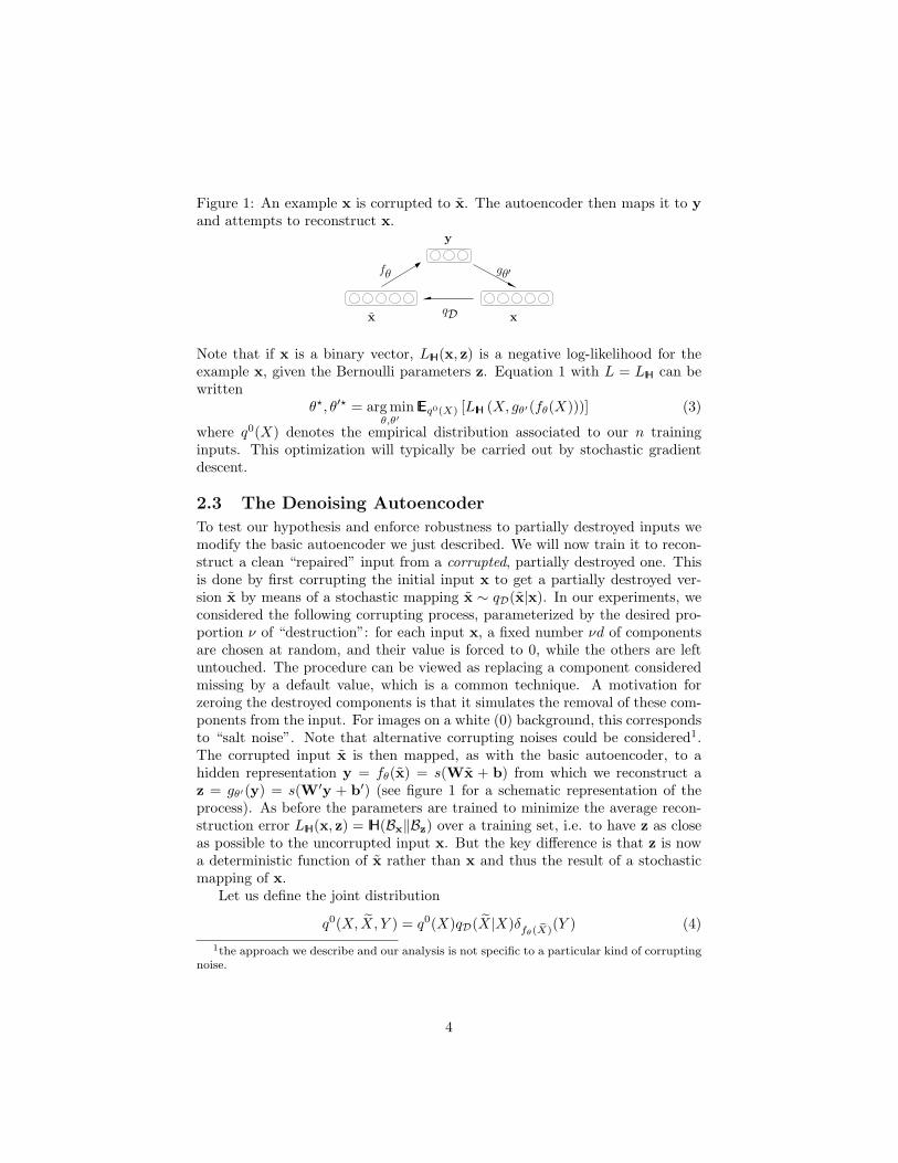
Figure 1: An example x is corrupted to x. The autoencoder then maps it to yand attempts to reconstruct x.

qD

fθ

x x

y

gθ′

Note that if x is a binary vector, LIH(x, z) is a negative log-likelihood for theexample x, given the Bernoulli parameters z. Equation 1 with L = LIH can bewritten

θ?, θ′? = arg minθ,θ′

EEq0(X) [LIH (X, gθ′(fθ(X)))] (3)

where q0(X) denotes the empirical distribution associated to our n traininginputs. This optimization will typically be carried out by stochastic gradientdescent.

2.3 The Denoising Autoencoder

To test our hypothesis and enforce robustness to partially destroyed inputs wemodify the basic autoencoder we just described. We will now train it to recon-struct a clean “repaired” input from a corrupted, partially destroyed one. Thisis done by first corrupting the initial input x to get a partially destroyed ver-sion x by means of a stochastic mapping x ∼ qD(x|x). In our experiments, weconsidered the following corrupting process, parameterized by the desired pro-portion ν of “destruction”: for each input x, a fixed number νd of componentsare chosen at random, and their value is forced to 0, while the others are leftuntouched. The procedure can be viewed as replacing a component consideredmissing by a default value, which is a common technique. A motivation forzeroing the destroyed components is that it simulates the removal of these com-ponents from the input. For images on a white (0) background, this correspondsto “salt noise”. Note that alternative corrupting noises could be considered1.The corrupted input x is then mapped, as with the basic autoencoder, to ahidden representation y = fθ(x) = s(Wx + b) from which we reconstruct az = gθ′(y) = s(W′y + b′) (see figure 1 for a schematic representation of theprocess). As before the parameters are trained to minimize the average recon-struction error LIH(x, z) = IH(Bx‖Bz) over a training set, i.e. to have z as closeas possible to the uncorrupted input x. But the key difference is that z is nowa deterministic function of x rather than x and thus the result of a stochasticmapping of x.

Let us define the joint distribution

q0(X, X, Y ) = q0(X)qD(X|X)δfθ( eX)(Y ) (4)1the approach we describe and our analysis is not specific to a particular kind of corrupting

noise.

4

where δu(v) puts mass 0 when u 6= v. Thus Y is a deterministic function ofX. q0(X, X, Y ) is parameterized by θ. The objective function minimized bystochastic gradient descent becomes:

arg minθ,θ′

EEq0(X, eX)

[LIH

(X, gθ′(fθ(X))

)]. (5)

So from the point of view of the stochastic gradient descent algorithm, in ad-dition to picking an input sample from the training set, we will also produce arandom corrupted version of it, and take a gradient step towards reconstructingthe uncorrupted version from the corrupted version. Note that in this way, theautoencoder cannot learn the identity, unlike the basic autoencoder, thus re-moving the constraint that d′ < d or the need to regularize specifically to avoidsuch a trivial solution.

2.4 Layer-wise Initialization and Fine Tuning

The basic autoencoder has been used as a building block to train deep net-works (Bengio et al., 2007), with the representation of the k-th layer used asinput for the (k +1)-th, and the (k +1)-th layer trained after the k-th has beentrained. After a few layers have been trained, the parameters are used as initial-ization for a network optimized with respect to a supervised training criterion.This greedy layer-wise procedure has been shown to yield significantly betterlocal minima than random initialization of deep networks (Bengio et al., 2007),achieving better generalization on a number of tasks (Larochelle et al., 2007).

The procedure to train a deep network using the denoising autoencoder issimilar. The only difference is how each layer is trained, i.e., to minimize thecriterion in eq. 5 instead of eq. 3. Note that the corruption process qD is onlyused during training, but not for propagating representations from the raw inputto higher-level representations. Note also that when layer k is trained, it receivesas input the uncorrupted output of the previous layers.

3 Relationship to Other Approaches

Our training procedure for the denoising autoencoder involves learning to re-cover a clean input from a corrupted version, a task known as denoising. Theproblem of image denoising, in particular, has been extensively studied in theimage processing community and many recent developments rely on machinelearning approaches (see e.g. Roth and Black (2005); Elad and Aharon (2006);Hammond and Simoncelli (2007)). A particular form of gated autoencoders hasalso been used for denoising in Memisevic (2007). Denoising using autoencoderswas actually introduced much earlier (LeCun, 1987; Gallinari et al., 1987), asan alternative to Hopfield models (Hopfield, 1982). Our objective however isfundamentally different from that of developing a competitive image denoisingalgorithm. We investigate explicit robustness to corrupting noise only as a cri-terion to guide the learning of suitable intermediate representations, with the

5

goal to build a better general purpose learning algorithm. Thus our corrup-tion+denoising procedure is applied not only on the input, but also recursivelyto intermediate representations. It is not specific to images and does not useprior knowledge of image topology.

Whereas the proposed approach does not rely on prior knowledge, it bearsresemblance to the well known technique of augmenting the training data withstochastically “transformed” patterns. But again we do not rely on prior knowl-edge. Moreover we only use the corrupted patterns to optimize an unsupervisedcriterion, as an initialization step.

There are also similarities with the work of (Doi et al., 2006) on robustcoding over noisy channels. In their framework, a linear encoder is to encodea clean input for optimal transmission over a noisy channel to a decoder thatreconstructs the input. This work was later extended to robustness to noise inthe input, in a proposal for a model of retinal coding (Doi & Lewicki, 2007).Though some of the inspiration behind our work comes from neural codingand computation, our goal is not to account for experimental data of neuronalactivity as in (Doi & Lewicki, 2007). Also, the non-linearity of our denoisingautoencoder is crucial for its use in initializing a deep neural network.

It may be objected that, if our goal is to handle missing values correctly,we could have more naturally defined a proper latent variable generative model,and infer the posterior over the latent (hidden) representation in the presenceof missing inputs. But this usually requires a costly marginalization2 which hasto be carried out for each new example. By contrast, our approach tries to learna fast and robust deterministic mapping fθ from examples of already corruptedinputs. The burden is on learning such a constrained mapping during training,rather than on unconstrained inference at use time. We expect this may forcethe model to capture implicit invariances in the data, and result in interestingfeatures. Also note that in section 4.4 we will see how our learning algorithmfor the denoising autoencoder can be viewed as a form of variational inferencein a particular generative model.

4 Analysis of the Denoising Autoencoder

The above intuitive motivation for the denoising autoencoder was given with theperspective of discovering robust representations. In the following, which canbe skipped without hurting the remainder of the paper, we try to gain insightby considering several alternative perspectives on the algorithm.

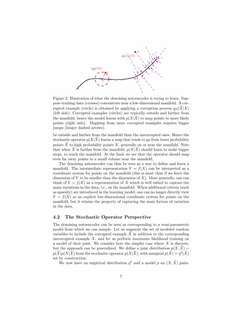
4.1 Manifold Learning Perspective

The process of mapping a corrupted example to an uncorrupted one can bevisualized in Figure 2, with a low-dimensional manifold near which the dataconcentrate. We learn a stochastic operator p(X|X) that maps an X to an X,p(X|X) = Bgθ′ (fθ( eX))(X). The corrupted examples will be much more likely to

2as in the case of RBMs, where it is exponential in the number of missing values

6

x

x

x

x

qD(x|x)

gθ′(fθ(x))

Figure 2: Illustration of what the denoising autoencoder is trying to learn. Sup-pose training data (crosses) concentrate near a low-dimensional manifold. A cor-rupted example (circle) is obtained by applying a corruption process qD(X|X)(left side). Corrupted examples (circles) are typically outside and farther fromthe manifold, hence the model learns with p(X|X) to map points to more likelypoints (right side). Mapping from more corrupted examples requires biggerjumps (longer dashed arrows).

be outside and farther from the manifold than the uncorrupted ones. Hence thestochastic operator p(X|X) learns a map that tends to go from lower probabilitypoints X to high probability points X, generally on or near the manifold. Notethat when X is farther from the manifold, p(X|X) should learn to make biggersteps, to reach the manifold. At the limit we see that the operator should mapeven far away points to a small volume near the manifold.

The denoising autoencoder can thus be seen as a way to define and learn amanifold. The intermediate representation Y = f(X) can be interpreted as acoordinate system for points on the manifold (this is most clear if we force thedimension of Y to be smaller than the dimension of X). More generally, one canthink of Y = f(X) as a representation of X which is well suited to capture themain variations in the data, i.e., on the manifold. When additional criteria (suchas sparsity) are introduced in the learning model, one can no longer directly viewY = f(X) as an explicit low-dimensional coordinate system for points on themanifold, but it retains the property of capturing the main factors of variationin the data.

4.2 The Stochastic Operator Perspective

The denoising autoencoder can be seen as corresponding to a semi-parametricmodel from which we can sample. Let us augment the set of modeled randomvariables to include the corrupted example X in addition to the correspondinguncorrupted example X, and let us perform maximum likelihood training ona model of their joint. We consider here the simpler case where X is discrete,but the approach can be generalized. We define a joint distribution p(X, X) =p(X)p(X|X) from the stochastic operator p(X|X), with marginal p(X) = q0(X)set by construction.

We now have an empirical distribution q0 and a model p on (X, X) pairs.

7

Performing maximum likelihood on them or minimizing IDKL(q0(X, X)‖p(X, X))is a reasonable training objective, again yielding the denoising criterion in eq. 5.

As an additional motivation for minimizing IDKL(q0(X, X)‖p(X, X)), notethat as we minimize it (i.e., IDKL(q0(X, X)‖p(X, X)) → 0), the marginals of papproach those of q0, hence in particular

p(X) → q0(X),

i.e., training in this way corresponds to a semi-parametric model p(X) whichapproaches the empirical distribution q0(X). By applying the marginalizationdefinition for p(X), we see what the corresponding model is

p(X) =1n

n∑i=1

∑x

p(X|X = x)qD(x|xi) (6)

where xi is one of the n training examples. Note that only the parameters ofp(X|X) are optimized in this model. Note also that sampling from the model iseasy. We have thus see that the denoising autoencoder learns a semi-parametricmodel which can be sampled from, based on the stochastic operator p(X|X).

What would happen if we were to apply this operator repeatedly? Thatwould define a chain pk(X) where p0(X = x) = q0(X = x), p1(X) = p(X)and pk(X) =

∑x p(X|X = x)pk−1(x). If the operator was ergodic (which

is plausible, following the above argumentation), its fixed point would defineyet another distribution π(X) = limk→∞ pk(X), of which the semi-parametricp(X) would be a first-order approximation. The advantage of this formulationis that π(X) is purely parametric: it does not explicitly depend on the empiricaldistribution q0.

4.3 Bottom-up Filtering, Information Theoretic Perspec-tive

In this section we adopt a bottom-up filtering viewpoint, and an information-theoretic perspective. Let X, X, Y be random variables representing respectivelyan input sample, a corrupted version of it, and the corresponding hidden rep-resentation, i.e. X ∼ q(X) (the true generating process for X), X ∼ qD(X|X),Y = fθ(X), with the associated joint q(X, X, Y ). Notice that it is defined withthe same dependency structure as q0(X, X, Y ), and the same conditionals X|Xand Y |X.

The role of the greedy layer initialization is to learn a non-linear filter thatyields a good representation of its input for the next layer. A good repre-sentation should retain a sufficient amount of “information” about its input,while we might at the same time encourage its marginal distribution to dis-play certain desirable properties. From this high level perspective, the filterwe learn, which has a fixed parameterized form with parameters θ, should beoptimized to realize a tradeoff between yielding a somewhat easier to modelmarginal distribution and retaining as much information as possible about the

8

input. This can be formalized as optimizing an objective function of the formarg maxθ {I(X;Y ) + λJ (Y )}, where J is a functional that induces some pref-erence over the marginal q(Y ), and hyper-parameter λ controls the tradeoff. Jcould for example encourage IDKL closeness to some reference prior distribution,or be some measure of sparsity or independence. In the present study, how-ever, we shall suppose that Y is only constrained by its dimensionality. Thiscorresponds to the case where J (Y ) is constant for all distributions (i.e. nopreference).

Let us thus examine only the first term. We have I(X;Y ) = IH(X)−IH(X|Y ).If we suppose the unknown input distribution q(X) fixed, IH(X) is a constant.Maximizing mutual information then amounts to maximizing −IH(X|Y ), i.e.

arg maxθ

I(X;Y ) = arg maxθ

−IH(X|Y )

maxθ−IH(X|Y ) = max

θEEq(X,Y )[log q(X|Y )]

= maxθ,p?

EEq(X,Y )[log p?(X|Y )]

where we optimize over all possible distributions p?. It is easy to show that themaximum is obtained for p?(X|Y ) = q(X|Y ). If instead we constrain p?(X|Y )to a given parametric form p(X|Y ) parameterized by θ′, we get a lower bound:

maxθ−IH(X|Y ) ≥ max

θ,θ′EEq(X,Y )[log p(X|Y )]

where we have an equality if ∃θ′ q(X|Y ) = p(X|Y ).In the case of an autoencoder with binary vector variable X, we can view the

top-down reconstruction as representing a p(X|Y ) = Bgθ′ (Y )(X). Optimizingfor the lower bound leads to:

maxθ,θ′

EEq(X,Y )[logBgθ′ (Y )(X)]

=maxθ,θ′

EEq(X, eX)[logBgθ′ (fθ( eX))(X)]

=minθ,θ′

EEq(X, eX)[LIH(X, gθ′(fθ(X)))]

where in the second line we use the fact that Y = fθ(X) deterministically. Thisis the criterion we use for training the autoencoder (eq. 5), but replacing thetrue generating process q by the empirical q0.

This shows that minimizing the expected reconstruction error amounts tomaximizing a lower bound on IH(X|Y ) and at the same time on the mutualinformation between input X and the hidden representation Y . Note that thisreasoning holds equally for the basic autoencoder, but with the denoising au-toencoder, we maximize the mutual information between X and Y even as Yis a function of corrupted input.

4.4 Top-down, Generative Model Perspective

In this section we try to recover the training criterion for our denoising autoen-coder (eq. 5) from a generative model perspective. Specifically we show that

9

training the denoising autoencoder as described in section 2.3 is equivalent tomaximizing a variational bound on a particular generative model.

Consider the generative model p(X, X, Y ) = p(Y )p(X|Y )p(X|X) wherep(X|Y ) = Bs(W′Y +b′) and p(X|X) = qD(X|X). p(Y ) is a uniform prior overY . This defines a generative model with parameter set θ′ = {W′,b′}. We willuse the previously defined q0(X, X, Y ) = q0(X)qD(X|X)δfθ( eX)(Y ) (equation 4)as an auxiliary model in the context of a variational approximation of the log-likelihood of p(X). Note that we abuse notation to make it lighter, and usethe same letters X, X and Y for different sets of random variables representingthe same quantity under different distributions: p or q0. Keep in mind thatwhereas we had the dependency structure X → X → Y for q or q0, we haveY → X → X for p.

Since p contains a corruption operation at the last generative stage, wepropose to fit p(X) to corrupted training samples. Performing maximum like-lihood fitting for samples drawn from q0(X) corresponds to minimizing thecross-entropy, or maximizing

H = maxθ′{−IH(q0(X)‖p(X))}

= maxθ′{EEq0( eX)[log p(X)]}. (7)

Let q?(X, Y |X) be a conditional density, the quantity L(q?, X) = EEq?(X,Y | eX)

[log p(X, eX,Y )

q?(X,Y | eX)

]is a lower bound on log p(X) since the following can be shown to be true forany q?:

log p(X) = L(q?, X) + IDKL(q?(X, Y |X)‖p(X, Y |X))

Also it is easy to verify that the bound is tight when q?(X, Y |X) = p(X, Y |X),where the IDKL becomes 0. We can thus write log p(X) = maxq? L(q?, X), andconsequently rewrite equation 7 as

H = maxθ′{EEq0( eX)[max

q?L(q?, X)]}

= maxθ′,q?

{EEq0( eX)[L(q?, X)]} (8)

where we moved the maximization outside of the expectation because an uncon-strained q?(X, Y |X) can in principle perfectly model the conditional distributionneeded to maximize L(q?, X) for any X. Now if we replace the maximizationover an unconstrained q? by the maximization over the parameters θ of our q0

(appearing in fθ that maps an x to a y), we get a lower bound on H

H ≥ maxθ′,θ

{EEq0( eX)[L(q0, X)]} (9)

10

Maximizing this lower bound, we find

arg maxθ,θ′

{EEq0( eX)[L(q0, X)]}

=arg maxθ,θ′

EEq0(X, eX,Y )

[log

p(X, X, Y )

q0(X, Y |X)

]=arg max

θ,θ′EEq0(X, eX,Y)

[log p(X, X, Y)

]+ EEq0( eX)

[IH[q0(X, Y |X)]

]=arg max

θ,θ′EEq0(X, eX,Y )

[log p(X, X, Y )

].

Note that θ only occurs in Y = fθ(X), and θ′ only occurs in p(X|Y ). The lastline is therefore obtained because q0(X|X) ∝ qD(X|X)q0(X) (none of whichdepends on (θ, θ′)), and q0(Y |X) is deterministic, i.e., its entropy is constant,irrespective of (θ, θ′). Hence the entropy of q0(X, Y |X) = q0(Y |X)q0(X|X),does not vary with (θ, θ′). Finally, following from above, we obtain our trainingcriterion (eq. 5):

arg maxθ,θ′

EEq0( eX)[L(q0, X)]

= arg maxθ,θ′

EEq0(X, eX,Y )[log[p(Y )p(X|Y )p(X|X)]]

= arg maxθ,θ′

EEq0(X, eX,Y )[log p(X|Y )]

= arg maxθ,θ′

EEq0(X, eX)[log p(X|Y = fθ(X))]

= arg minθ,θ′

EEq0(X, eX)

[LIH

(X, gθ′(fθ(X))

)]where the third line is obtained because (θ, θ′) have no influence on EEq0(X, eX,Y )[log p(Y )]

because we chose p(Y ) uniform, i.e. constant, nor on EEq0(X, eX)[log p(X|X)], andthe last line is obtained by inspection of the definition of LIH in eq. 2, whenp(X|Y = fθ(X)) is a Bgθ′ (fθ( eX)).

5 Experiments

We performed experiments with the proposed algorithm on the same benchmarkof classification problems used in (Larochelle et al., 2007)3. It contains differ-ent variations of the MNIST digit classification problem, with added factors ofvariation such as rotation (rot), addition of a background composed of randompixels (bg-rand) or made from patches extracted from a set of images (bg-img), orcombinations of these factors (rot-bg-img). These variations render the problems

3All the datasets for these problems were taken fromhttp://www.iro.umontreal.ca/∼lisa/icml2007.

11

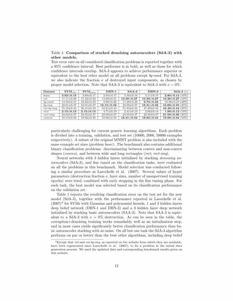
Table 1: Comparison of stacked denoising autoencoders (SdA-3) withother models.Test error rate on all considered classification problems is reported together witha 95% confidence interval. Best performer is in bold, as well as those for whichconfidence intervals overlap. SdA-3 appears to achieve performance superior orequivalent to the best other model on all problems except bg-rand. For SdA-3,we also indicate the fraction ν of destroyed input components, as chosen byproper model selection. Note that SAA-3 is equivalent to SdA-3 with ν = 0%.

Dataset SVMrbf SVMpoly DBN-1 SAA-3 DBN-3 SdA-3 (ν)

basic 3.03±0.15 3.69±0.17 3.94±0.17 3.46±0.16 3.11±0.15 2.80±0.14 (10%)rot 11.11±0.28 15.42±0.32 14.69±0.31 10.30±0.27 10.30±0.27 10.29±0.27 (10%)bg-rand 14.58±0.31 16.62±0.33 9.80±0.26 11.28±0.28 6.73±0.22 10.38±0.27 (40%)bg-img 22.61±0.37 24.01±0.37 16.15±0.32 23.00±0.37 16.31±0.32 16.68±0.33 (25%)rot-bg-img 55.18±0.44 56.41±0.43 52.21±0.44 51.93±0.44 47.39±0.44 44.49±0.44 (25%)rect 2.15±0.13 2.15±0.13 4.71±0.19 2.41±0.13 2.60±0.14 1.99±0.12 (10%)rect-img 24.04±0.37 24.05±0.37 23.69±0.37 24.05±0.37 22.50±0.37 21.59±0.36 (25%)convex 19.13±0.34 19.82±0.35 19.92±0.35 18.41±0.34 18.63±0.34 19.06±0.34 (10%)

particularly challenging for current generic learning algorithms. Each problemis divided into a training, validation, and test set (10000, 2000, 50000 examplesrespectively). A subset of the original MNIST problem is also included with thesame example set sizes (problem basic). The benchmark also contains additionalbinary classification problems: discriminating between convex and non-convexshapes (convex), and between wide and long rectangles (rect, rect-img).

Neural networks with 3 hidden layers initialized by stacking denoising au-toencoders (SdA-3), and fine tuned on the classification tasks, were evaluatedon all the problems in this benchmark. Model selection was conducted follow-ing a similar procedure as Larochelle et al. (2007). Several values of hyperparameters (destruction fraction ν, layer sizes, number of unsupervised trainingepochs) were tried, combined with early stopping in the fine tuning phase. Foreach task, the best model was selected based on its classification performanceon the validation set.

Table 1 reports the resulting classification error on the test set for the newmodel (SdA-3), together with the performance reported in Larochelle et al.(2007)4 for SVMs with Gaussian and polynomial kernels, 1 and 3 hidden layersdeep belief network (DBN-1 and DBN-3) and a 3 hidden layer deep networkinitialized by stacking basic autoencoders (SAA-3). Note that SAA-3 is equiv-alent to a SdA-3 with ν = 0% destruction. As can be seen in the table, thecorruption+denoising training works remarkably well as an initialization step,and in most cases yields significantly better classification performance than ba-sic autoencoder stacking with no noise. On all but one task the SdA-3 algorithmperforms on par or better than the best other algorithms, including deep belief

4Except that rot and rot-bg-img, as reported on the website from which they are available,have been regenerated since Larochelle et al. (2007), to fix a problem in the initial datageneration process. We used the updated data and corresponding benchmark results given onthis website.

12

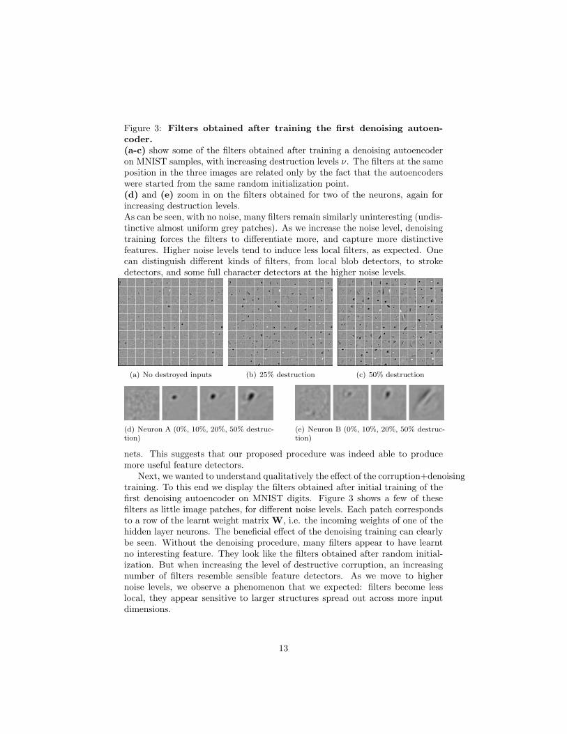
Figure 3: Filters obtained after training the first denoising autoen-coder.(a-c) show some of the filters obtained after training a denoising autoencoderon MNIST samples, with increasing destruction levels ν. The filters at the sameposition in the three images are related only by the fact that the autoencoderswere started from the same random initialization point.(d) and (e) zoom in on the filters obtained for two of the neurons, again forincreasing destruction levels.As can be seen, with no noise, many filters remain similarly uninteresting (undis-tinctive almost uniform grey patches). As we increase the noise level, denoisingtraining forces the filters to differentiate more, and capture more distinctivefeatures. Higher noise levels tend to induce less local filters, as expected. Onecan distinguish different kinds of filters, from local blob detectors, to strokedetectors, and some full character detectors at the higher noise levels.

(a) No destroyed inputs (b) 25% destruction (c) 50% destruction

(d) Neuron A (0%, 10%, 20%, 50% destruc-tion)

(e) Neuron B (0%, 10%, 20%, 50% destruc-tion)

nets. This suggests that our proposed procedure was indeed able to producemore useful feature detectors.

Next, we wanted to understand qualitatively the effect of the corruption+denoisingtraining. To this end we display the filters obtained after initial training of thefirst denoising autoencoder on MNIST digits. Figure 3 shows a few of thesefilters as little image patches, for different noise levels. Each patch correspondsto a row of the learnt weight matrix W, i.e. the incoming weights of one of thehidden layer neurons. The beneficial effect of the denoising training can clearlybe seen. Without the denoising procedure, many filters appear to have learntno interesting feature. They look like the filters obtained after random initial-ization. But when increasing the level of destructive corruption, an increasingnumber of filters resemble sensible feature detectors. As we move to highernoise levels, we observe a phenomenon that we expected: filters become lesslocal, they appear sensitive to larger structures spread out across more inputdimensions.

13

6 Conclusion and Future Work

We have introduced a very simple training principle for autoencoders, based onthe objective of undoing a corruption process. This is motivated by the goal oflearning representations of the input that are robust to small irrelevant changesin input. Several perspectives also help to motivate it from a manifold learningperspective and from the perspective of a generative model.

This principle can be used to train and stack autoencoders to initialize adeep neural network. A series of image classification experiments were per-formed to evaluate this new training principle. The empirical results supportthe following conclusions: unsupervised initialization of layers with an explicitdenoising criterion helps to capture interesting structure in the input distribu-tion. This in turn leads to intermediate representations much better suited forsubsequent learning tasks such as supervised classification. The experimentalresults with Deep Belief Networks (whose layers are initialized as RBMs) sug-gest that RBMs may also encapsulate a form of robustness in the representationsthey learn, possibly because of their stochastic nature, which introduces noisein the representation during training. Future work inspired by this observationshould investigate other types of corruption process, not only of the input butof the representation itself as well.

References

Bengio, Y. (2007). Learning deep architectures for AI (Technical Report 1312).Universite de Montreal, dept. IRO.

Bengio, Y., Lamblin, P., Popovici, D., & Larochelle, H. (2007). Greedy layer-wise training of deep networks. Advances in Neural Information ProcessingSystems 19 (pp. 153–160). MIT Press.

Bengio, Y., & Le Cun, Y. (2007). Scaling learning algorithms towards AI. InL. Bottou, O. Chapelle, D. DeCoste and J. Weston (Eds.), Large scale kernelmachines. MIT Press.

Doi, E., Balcan, D. C., & Lewicki, M. S. (2006). A theoretical analysis ofrobust coding over noisy overcomplete channels. In Y. Weiss, B. Scholkopfand J. Platt (Eds.), Advances in neural information processing systems 18,307–314. Cambridge, MA: MIT Press.

Doi, E., & Lewicki, M. S. (2007). A theory of retinal population coding. NIPS(pp. 353–360). MIT Press.

Elad, M., & Aharon, M. (2006). Image denoising via sparse and redundantrepresentations over learned dictionaries. IEEE Transactions on Image Pro-cessing, 15, 3736–3745.

Gallinari, P., LeCun, Y., Thiria, S., & Fogelman-Soulie, F. (1987). Memoiresassociatives distribuees. Proceedings of COGNITIVA 87. Paris, La Villette.

14

Hammond, D., & Simoncelli, E. (2007). A machine learning framework for adap-tive combination of signal denoising methods. 2007 International Conferenceon Image Processing (pp. VI: 29–32).

Hinton, G. (1989). Connectionist learning procedures. Artificial Intelligence,40, 185–234.

Hinton, G., & Salakhutdinov, R. (2006). Reducing the dimensionality of datawith neural networks. Science, 313, 504–507.

Hinton, G. E., Osindero, S., & Teh, Y. (2006). A fast learning algorithm fordeep belief nets. Neural Computation, 18, 1527–1554.

Hopfield, J. (1982). Neural networks and physical systems with emergent collec-tive computational abilities. Proceedings of the National Academy of Sciences,USA, 79.

Larochelle, H., Erhan, D., Courville, A., Bergstra, J., & Bengio, Y. (2007).An empirical evaluation of deep architectures on problems with many factorsof variation. Twenty-fourth International Conference on Machine Learning(ICML’2007).

LeCun, Y. (1987). Modeles connexionistes de l’apprentissage. Doctoral disser-tation, Universite de Paris VI.

Lee, H., Ekanadham, C., & Ng, A. (2008). Sparse deep belief net model for visualarea V2. In J. Platt, D. Koller, Y. Singer and S. Roweis (Eds.), Advances inneural information processing systems 20. Cambridge, MA: MIT Press.

McClelland, J., Rumelhart, D., & the PDP Research Group (1986). Paralleldistributed processing: Explorations in the microstructure of cognition, vol. 2.Cambridge: MIT Press.

Memisevic, R. (2007). Non-linear latent factor models for revealing structurein high-dimensional data. Doctoral dissertation, Departement of ComputerScience, University of Toronto, Toronto, Ontario, Canada.

Ranzato, M., Boureau, Y.-L., & LeCun, Y. (2008). Sparse feature learning fordeep belief networks. In J. Platt, D. Koller, Y. Singer and S. Roweis (Eds.),Advances in neural information processing systems 20. Cambridge, MA: MITPress.

Ranzato, M., Poultney, C., Chopra, S., & LeCun, Y. (2007). Efficient learningof sparse representations with an energy-based model. Advances in NeuralInformation Processing Systems (NIPS 2006). MIT Press.

Roth, S., & Black, M. (2005). Fields of experts: a framework for learning imagepriors. IEEE Conference on Computer Vision and Pattern Recognition (pp.860–867).

15

Utgoff, P., & Stracuzzi, D. (2002). Many-layered learning. Neural Computation,14, 2497–2539.

16