ee 380 linear control systems lecture 4courses.ee.psu.edu/schiano/ee380/lectures/l4_ee380_f14.pdfee...
TRANSCRIPT
EE 380 Fall 2014Lecture 4.
EE 380
Linear Control Systems
Lecture 4
Professor Jeffrey SchianoDepartment of Electrical Engineering
1

EE 380 Fall 2014Lecture 4.
Lecture 4 Topics
• State-Space Representation– Advantages– Definitions– Transfer function from State-Space Matrices
• Example
2

EE 380 Fall 2014Lecture 4.
Advantages• Facilitates the use of linear algebra tools in the design and
analysis of feedback control systems– Nonlinear systems– Time-varying systems
• Easily represents multiple-input multi-output (MIMO) systems
• Provides a complete internal model of the plant dynamics– Pole-zero cancellations in the transfer function
(input/output ) description may hide poorly damped (oscillatory) or unstable modes
3
EE 380 Fall 2014Lecture 4.
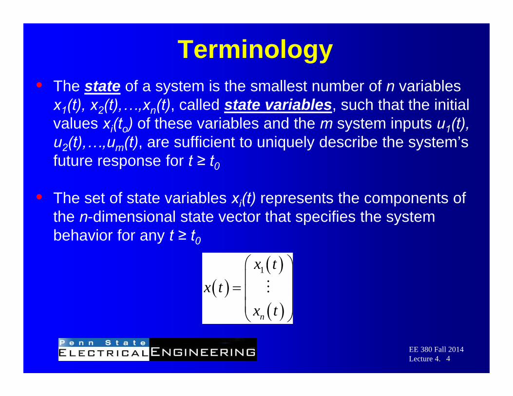
Terminology• The state of a system is the smallest number of n variables
x1(t), x2(t),…,xn(t), called state variables, such that the initial values xi(to) of these variables and the m system inputs u1(t), u2(t),…,um(t), are sufficient to uniquely describe the system’s future response for t ≥ t0
• The set of state variables xi(t) represents the components of the n-dimensional state vector that specifies the system behavior for any t ≥ t0
4
1
n
x tx t
x t

EE 380 Fall 2014Lecture 4.
Terminology• State space defines an n-dimensional space in which the
components of the state vector represent its coordinate axis
• State trajectory defines the path of the state vector x(t) as it evolves with time. State space and state trajectory in the two-dimensional case (n=2) are referred to as the phase plane and phase trajectory
• The state equations are a coupled set of n first-order differential equations expressed in terms of the state variables
5
EE 380 Fall 2014Lecture 4.
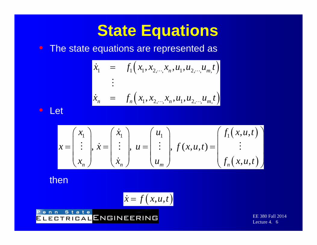
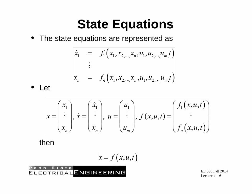
State Equations• The state equations are represented as
• Let
then
6
1 1 1 2, , 1 2, , ,
1 2, , 1 2, , ,
, , ,
, , ,
n m
n n n m
x f x x x u u u t
x f x x x u u u t
, ,x f x u t
1 1 1 1 , ,, , , ( , , )
, ,n n m n
x x u f x u tx x u f x u t
x x u f x u t

EE 380 Fall 2014Lecture 4.
Output Equations• The output equations are represented as
• Let
then
7
1 1 1 2, , 1 2, , ,
1 2, , 1 2, , ,
, , ,
, , ,
n m
r r n m
y g x x x u u u t
y g x x x u u u t
, ,y g x u t
1 1 , ,, ( , , )
, ,r r
y g x u ty g x u t
y g x u t

EE 380 Fall 2014Lecture 4.
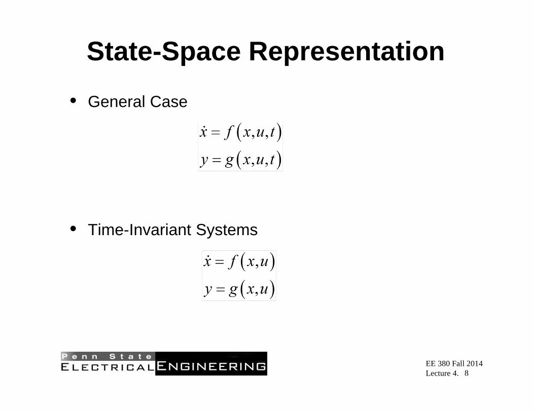
State-Space Representation• General Case
• Time-Invariant Systems
8
, ,
, ,
x f x u t
y g x u t
,
,
x f x u
y g x u

EE 380 Fall 2014Lecture 4.
Linear System• Linear Time-Varying Systems
• Linear Time-Invariant Systems
• Dimensions
9
x F t x G t u
y H t x J t u
x Ax Buy Cx Du
1 1 1, ,n m rx u y
x A t x B t u
y C t x D t u
x Fx Guy Hx Ju
, , ,n n n m r n r mA B C D , , ,n n n m r n r mF G H J

EE 380 Fall 2014Lecture 4.
Transfer Function Representation• For a LTI system represented by the state-space model
the transfer function representation is
10
,x Fx Guy Hx Ju
1
transfer function
Y s H sI F G J U s
,x Ax Buy Cx Du
1
transfer function
Y s C sI A B D U s
EE 380 Fall 2014Lecture 4.
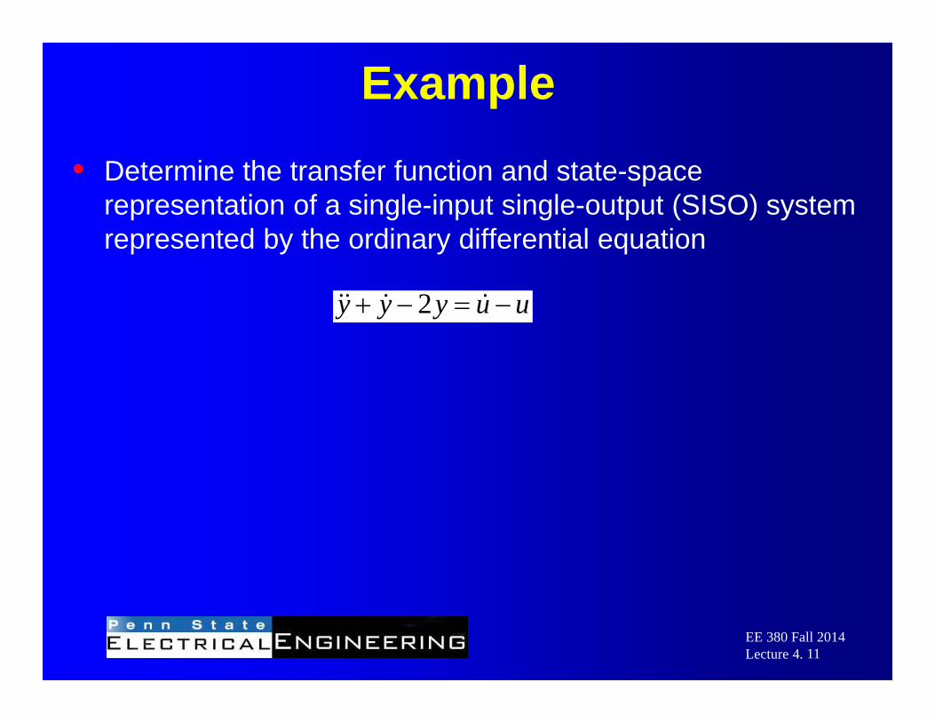
Example• Determine the transfer function and state-space
representation of a single-input single-output (SISO) system represented by the ordinary differential equation
11
2y y y u u

EE 380 Fall 2014Lecture 4.
Solution
12

EE 380 Fall 2014Lecture 4.
Solution
13

EE 380 Fall 2014Lecture 4.
Solution
14

EE 380 Fall 2014Lecture 4.
EE 380
Linear Control Systems
Lecture 4
Professor Jeffrey SchianoDepartment of Electrical Engineering
1
EE 380 Fall 2014Lecture 4.
Lecture 4 Topics
• State-Space Representation– Advantages– Definitions– Transfer function from State-Space Matrices
• Example
2
EE 380 Fall 2014Lecture 4.
Advantages• Facilitates the use of linear algebra tools in the design and
analysis of feedback control systems– Nonlinear systems– Time-varying systems
• Easily represents multiple-input multi-output (MIMO) systems
• Provides a complete internal model of the plant dynamics– Pole-zero cancellations in the transfer function
(input/output ) description may hide poorly damped (oscillatory) or unstable modes
3

EE 380 Fall 2014Lecture 4.
Terminology• The state of a system is the smallest number of n variables
x1(t), x2(t),…,xn(t), called state variables, such that the initial values xi(to) of these variables and the m system inputs u1(t), u2(t),…,um(t), are sufficient to uniquely describe the system’s future response for t ≥ t0
• The set of state variables xi(t) represents the components of the n-dimensional state vector that specifies the system behavior for any t ≥ t0
4

EE 380 Fall 2014Lecture 4.
Terminology• State space defines an n-dimensional space in which the
components of the state vector represent its coordinate axis
• State trajectory defines the path of the state vector x(t) as it evolves with time. State space and state trajectory in the two-dimensional case (n=2) are referred to as the phase plane and phase trajectory
• The state equations are a coupled set of n first-order differential equations expressed in terms of the state variables
5
EE 380 Fall 2014Lecture 4.
State Equations• The state equations are represented as
• Let
then
6

EE 380 Fall 2014Lecture 4.
Output Equations• The output equations are represented as
• Let
then
7
EE 380 Fall 2014Lecture 4.
State-Space Representation• General Case
• Time-Invariant Systems
8

EE 380 Fall 2014Lecture 4.
Linear System• Linear Time-Varying Systems
• Linear Time-Invariant Systems
• Dimensions
9

EE 380 Fall 2014Lecture 4.
Transfer Function Representation• For a LTI system represented by the state-space model
the transfer function representation is
10

EE 380 Fall 2014Lecture 4.
Example• Determine the transfer function and state-space
representation of a single-input single-output (SISO) system represented by the ordinary differential equation
11

EE 380 Fall 2014Lecture 4.
Solution
12
EE 380 Fall 2014Lecture 4.
Solution
13

EE 380 Fall 2014Lecture 4.
Solution
14