Editorial Manager(tm) for Journal of Computational Physics

Manuscript Draft

Manuscript Number:

Title: Efficient Algorithms for Discrete Lattice Calculations

Article Type: Regular Article

Keywords: lattice algorithms; lattice reduction; nearest neighbor; cluster computation;

quasicontinuum

Corresponding Author: Professor Ellad B Tadmor, Ph.D.

Corresponding Author's Institution: University of Minnesota

First Author: Marcel Arndt, Ph.D.

Order of Authors: Marcel Arndt, Ph.D.; Viacheslav Sorkin, Ph.D.; Ellad B Tadmor, Ph.D.

1 2 3 4 5 6 7 8 9 10 11 12 13 14 15 16 17 18 19 20 21 22 23 24 25 26 27 28 29 30 31 32 33 34 35 36 37 38 39 40 41 42 43 44 45 46 47 48 49 50 51 52 53 54 55 56 57 58 59 60 61 62 63 64 65

Efficient Algorithms for Discrete Lattice Calculations

M. Arndt a V. Sorkin b E. B. Tadmor b,∗aSchool of Mathematics, University of Minnesota, Minneapolis, MN 55455, USAbDepartment of Aerospace Engineering and Mechanics, University of Minnesota,

Minneapolis, MN 55455, USA

Abstract

We discuss algorithms for lattice based computations, in particular lattice reduction, the de-tection of nearest neighbors, and the computation of clusters of nearest neighbors. We focuson algorithms that are most efficient for low spatial dimensions (typically d = 2, 3) and inputdata within a reasonably limited range. This makes them most useful for physically oriented nu-merical simulations, for example of crystalline solids. Different solution strategies are discussed,formulated as algorithms, and numerically evaluated.

Key words: lattice algorithms, lattice reduction, nearest neighbor, cluster computation,quasicontinuumPACS: 02.60.Cb, 61.50.Ah

1. Introduction

Scientific computing often involves lattices and algorithms operating on them. For ex-ample, the atoms in a crystalline solid are arranged in the form of a lattice, and numericalcodes that simulate the behavior of such crystals need to perform many operations onthis lattice. This includes the identification of all atoms within a given radius of a latticesite for energy and force calculations and the location of the nearest lattice site to an ar-bitrary point. In particular, the current work was motivated by lattice algorithms neededfor the quasicontinuum (QC) method [12–14]. Lattices are also used in other physicalapplications, such as the Ising model [8], lattice monte carlo [6], lattice protein foldingalgorithms [15], as well as in more abstract settings, such as integer linear programming

∗ Corresponding author.Email address: tadmor@aem.umn.edu (E. B. Tadmor).

Preprint submitted to Elsevier 29 September 2008

manuscript

1 2 3 4 5 6 7 8 9 10 11 12 13 14 15 16 17 18 19 20 21 22 23 24 25 26 27 28 29 30 31 32 33 34 35 36 37 38 39 40 41 42 43 44 45 46 47 48 49 50 51 52 53 54 55 56 57 58 59 60 61 62 63 64 65

problems in operations research, lattice-based cryptography and communication theory[1].

Lattice algorithms and their computational complexity have been intensively studiedfrom the algebraic point of view. This resulted in the development of highly-sophisticatedalgorithms that have good scaling properties as the spatial dimension d gets large or thelattice gets highly distorted. For an overview of such lattice algorithm, see, e.g., [1, 5].A more general classical reference for lattices and their properties is [2]. However, thesesophisticated algorithms are not always optimal for many applications that are orientedmore towards physics or engineering, where the spatial dimension d is typically low(mostly d = 2, 3), and lattice distortions are typically limited to a physically-relevantrange so that the scaling properties of the algorithms do not come into play. In thesecases, simpler approaches that are significantly easier to implement can be superior tothe more sophisticated techniques.

This paper describes lattice algorithms that are tailored to practical physical applica-tions in numerical simulation and evaluates their performance on a set of test problems.The authors feel that there is a gap between the mathematically complex algorithmsmentioned above and the naive “brute-force” approaches that are often used in practi-cal applications. The purpose of this paper is to fill this gap for certain common latticeproblems and to make algorithms readily-available for application.

We deal with three problems: lattice reduction, detection of nearest lattice sites, andcomputation of clusters of nearest neighbors. As noted above, this study was motivatedby the QC method, nevertheless, these problems have been formulated in a general wayto make them applicable and useful for a large variety of applications. We consider bothsimple lattices and multilattices, also called “lattices with a basis”, which correspond toa set of inter-penetrating simple lattices.

A key starting point for many algorithms is a suitable lattice reduction that determinesan optimal set of lattice vectors that can considerably accelerate subsequent operations.In Section 2, we discuss two variants of lattice reduction: the classical LLL reduction [7]that provides approximate, globally-optimized lattice vectors and a pairwise reductionapproach that results in lattice vectors that are pairwise optimal but not necessarilyglobally optimal. The advantages and disadvantages of these approaches are discussed.Numerical studies of their performance appear in subsequent sections where they areincorporated into other algorithms.

Section 3 deals with the detection of nearest lattice sites, also known as the closestvector problem, for both simple lattices and multilattices. We discuss two strategies: anaive brute-force algorithm and a new approach which we refer to as the short-list algo-

rithm. The latter is based on investing some computation time in advance to determinea small set of candidate lattice sites that is subsequently used to speed up the actualprocess of neighbor detection. This is advantageous when multiple lattice sites need tobe detected for the same lattice structure. Both algorithms are evaluated numerically.

In Section 4, we discuss the computation of clusters of nearest neighbors, i.e., determi-nation of the set of all lattice sites within a given radius of a specified lattice site for bothsimple lattices and multilattices. This can be seen as a variation of the closest vectorproblem in which only the single nearest lattice site is detected. We discuss and numeri-cally assess the performance of two strategies that we developed: the shell algorithm andthe on-the-fly algorithm.

Concluding remarks are given in Section 5. The appendix contains proofs and technical

2

1 2 3 4 5 6 7 8 9 10 11 12 13 14 15 16 17 18 19 20 21 22 23 24 25 26 27 28 29 30 31 32 33 34 35 36 37 38 39 40 41 42 43 44 45 46 47 48 49 50 51 52 53 54 55 56 57 58 59 60 61 62 63 64 65

details omitted from the main text in order not to interrupt the flow of reading.

2. Lattice Reduction

A simple lattice L in d-dimensional space is an infinite discrete set of points that areinteger linear combinations of lattice vectors, ai ∈ R

d, for i = 1, . . . , d, 1

L =

d∑

i=1

aini : ni ∈ Z

= An : n ∈ Zd. (1)

In the second term, we subsume the lattice vectors as the column vectors of the matrixA ∈ R

d×d, i.e., A = (a1 · · ·ad). To avoid degenerate lattices, we require the latticevectors ai to be linearly independent, or equivalently the matrix A to be invertible.

The lattice definition in (1) is not unique because the lattice vectors are not uniquelydetermined. Two lattices spanned by A and A coincide,

An : n ∈ Zd = An : n ∈ Z

d, (2)

if and only if the matrix M = A−1A is unimodular, i.e., M and its inverse M−1 =

A−1

A are integer matrices, or equivalently if M is an integer matrix with determinant±1, i.e., |detM | = 1.

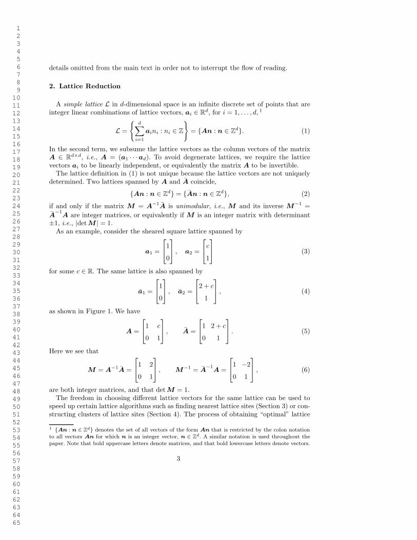
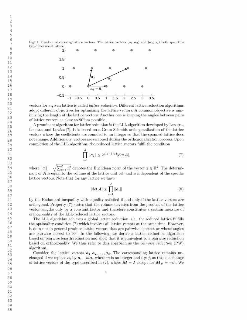
As an example, consider the sheared square lattice spanned by

a1 =

1

0

, a2 =

c

1

(3)

for some c ∈ R. The same lattice is also spanned by

a1 =

1

0

, a2 =

2 + c

1

, (4)

as shown in Figure 1. We have

A =

1 c

0 1

, A =

1 2 + c

0 1

. (5)

Here we see that

M = A−1A =

1 2

0 1

, M−1 = A−1

A =

1 −2

0 1

, (6)

are both integer matrices, and that det M = 1.The freedom in choosing different lattice vectors for the same lattice can be used to

speed up certain lattice algorithms such as finding nearest lattice sites (Section 3) or con-structing clusters of lattice sites (Section 4). The process of obtaining “optimal” lattice

1 An : n ∈ Zd denotes the set of all vectors of the form An that is restricted by the colon notation

to all vectors An for which n is an integer vector, n ∈ Zd. A similar notation is used throughout the

paper. Note that bold uppercase letters denote matrices, and that bold lowercase letters denote vectors.

3

1 2 3 4 5 6 7 8 9 10 11 12 13 14 15 16 17 18 19 20 21 22 23 24 25 26 27 28 29 30 31 32 33 34 35 36 37 38 39 40 41 42 43 44 45 46 47 48 49 50 51 52 53 54 55 56 57 58 59 60 61 62 63 64 65

Fig. 1. Freedom of choosing lattice vectors. The lattice vectors (a1, a2) and (a1, a2) both span thistwo-dimensional lattice.

−1 −0.5 0 0.5 1 1.5 2 2.5 3 3.5−0.5

0

0.5

1

1.5

2

a1 = a1

a2 a2

vectors for a given lattice is called lattice reduction. Different lattice reduction algorithmsadopt different objectives for optimizing the lattice vectors. A common objective is min-imizing the length of the lattice vectors. Another one is keeping the angles between pairsof lattice vectors as close to 90 as possible.

A prominent algorithm for lattice reduction is the LLL algorithm developed by Lenstra,Lenstra, and Lovasz [7]. It is based on a Gram-Schmidt orthogonalization of the latticevectors where the coefficients are rounded to an integer so that the spanned lattice doesnot change. Additionally, vectors are swapped during the orthogonalization process. Uponcompletion of the LLL algorithm, the reduced lattice vectors fulfil the condition

d∏

i=1

‖ai‖ ≤ 2d(d−1)/4|detA|, (7)

where ‖x‖ =

√

∑di=1 x2

i denotes the Euclidean norm of the vector x ∈ Rd. The determi-

nant of A is equal to the volume of the lattice unit cell and is independent of the specificlattice vectors. Note that for any lattice we have

|detA| ≤d

∏

i=1

‖ai‖ (8)

by the Hadamard inequality with equality satisfied if and only if the lattice vectors areorthogonal. Property (7) states that the volume deviates from the product of the latticevector lengths only by a constant factor and therefore constitutes a certain measure oforthogonality of the LLL-reduced lattice vectors.

The LLL algorithm achieves a global lattice reduction, i.e., the reduced lattice fulfillsthe optimality condition (7) which involves all lattice vectors at the same time. However,it does not in general produce lattice vectors that are pairwise shortest or whose anglesare pairwise closest to 90. In the following, we derive a lattice reduction algorithmbased on pairwise length reduction and show that it is equivalent to a pairwise reductionbased on orthogonality. We thus refer to this approach as the pairwise reduction (PW)algorithm.

Consider the lattice vectors a1, a2, . . . , ad. The corresponding lattice remains un-changed if we replace ai by ai −maj where m is an integer and i 6= j, as this is a changeof lattice vectors of the type described in (2), where M = I except for M ji = −m. We

4

1 2 3 4 5 6 7 8 9 10 11 12 13 14 15 16 17 18 19 20 21 22 23 24 25 26 27 28 29 30 31 32 33 34 35 36 37 38 39 40 41 42 43 44 45 46 47 48 49 50 51 52 53 54 55 56 57 58 59 60 61 62 63 64 65

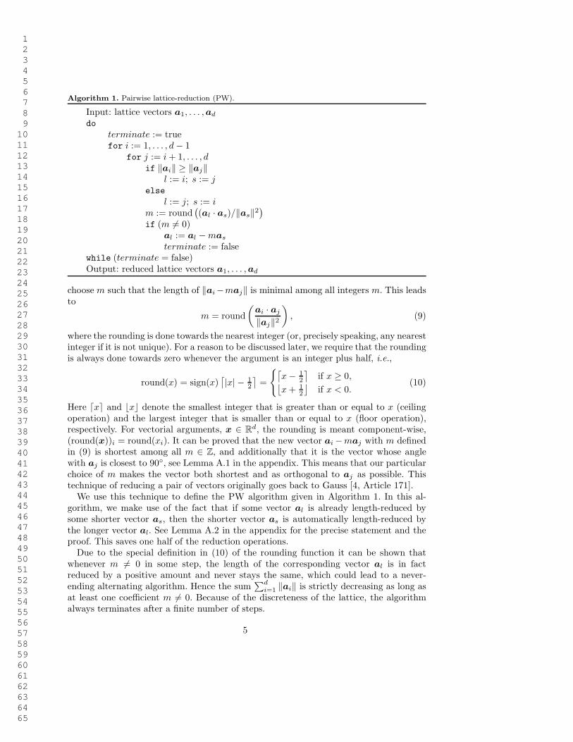
Algorithm 1. Pairwise lattice-reduction (PW).

Input: lattice vectors a1, . . . , ad

do

terminate := truefor i := 1, . . . , d − 1

for j := i + 1, . . . , dif ‖ai‖ ≥ ‖aj‖

l := i; s := jelse

l := j; s := im := round

(

(al · as)/‖as‖2)

if (m 6= 0)al := al − mas

terminate := falsewhile (terminate = false)Output: reduced lattice vectors a1, . . . , ad

choose m such that the length of ‖ai−maj‖ is minimal among all integers m. This leadsto

m = round

(

ai · aj

‖aj‖2

)

, (9)

where the rounding is done towards the nearest integer (or, precisely speaking, any nearestinteger if it is not unique). For a reason to be discussed later, we require that the roundingis always done towards zero whenever the argument is an integer plus half, i.e.,

round(x) = sign(x)⌈

|x| − 12

⌉

=

⌈

x − 12

⌉

if x ≥ 0,⌊

x + 12

⌋

if x < 0.(10)

Here ⌈x⌉ and ⌊x⌋ denote the smallest integer that is greater than or equal to x (ceilingoperation) and the largest integer that is smaller than or equal to x (floor operation),respectively. For vectorial arguments, x ∈ R

d, the rounding is meant component-wise,(round(x))i = round(xi). It can be proved that the new vector ai −maj with m definedin (9) is shortest among all m ∈ Z, and additionally that it is the vector whose anglewith aj is closest to 90, see Lemma A.1 in the appendix. This means that our particularchoice of m makes the vector both shortest and as orthogonal to aj as possible. Thistechnique of reducing a pair of vectors originally goes back to Gauss [4, Article 171].

We use this technique to define the PW algorithm given in Algorithm 1. In this al-gorithm, we make use of the fact that if some vector al is already length-reduced bysome shorter vector as, then the shorter vector as is automatically length-reduced bythe longer vector al. See Lemma A.2 in the appendix for the precise statement and theproof. This saves one half of the reduction operations.

Due to the special definition in (10) of the rounding function it can be shown thatwhenever m 6= 0 in some step, the length of the corresponding vector al is in factreduced by a positive amount and never stays the same, which could lead to a never-ending alternating algorithm. Hence the sum

∑di=1 ‖ai‖ is strictly decreasing as long as

at least one coefficient m 6= 0. Because of the discreteness of the lattice, the algorithmalways terminates after a finite number of steps.

5

1 2 3 4 5 6 7 8 9 10 11 12 13 14 15 16 17 18 19 20 21 22 23 24 25 26 27 28 29 30 31 32 33 34 35 36 37 38 39 40 41 42 43 44 45 46 47 48 49 50 51 52 53 54 55 56 57 58 59 60 61 62 63 64 65

The algorithm concludes with a set of lattice vectors that are pairwise reduced ac-cording to both length and angle. This means that subtracting an integer multiple ofone vector from another vector never reduces its length or brings the angle closer to90. However, it can be shown that this is not a global property, i.e., subtracting two ormore integer multiples at the same time could lead to an improvement. Obtaining a setof lattice vectors which is globally reduced in this sense is a considerably more difficulttask, and to the best knowledge of the authors, no efficient algorithm for arbitrary spacedimension d exists that does so.

It is worth noting that the technique used here is similar to the Euclidean Algorithmfor finding the greatest common divisor (gcd) of two positive integers. This similarity isdue to the fact that both lattice vectors and gcd share the same structure of invariance;two positive integers ni, nj have the same gcd as ni, nj if and only if

(ni nj) = (ni nj)M (11)

for some unimodular matrix M ; compare this to (2).

3. Nearest Lattice Site Detection

One problem that frequently occurs in many applications is the determination of thelattice site that is nearest to some given point x ∈ R

d in space, also known as theclosest vector problem. An example is mesh generation and mesh refinement within theQC method, where mesh nodes are constrained to occupy lattice sites. Whenever theinitial mesh is computed or the mesh is refined by adding nodes during automatic meshrefinement, the nodes must be moved to the nearest lattice site. The fast determinationof nearest lattice sites is therefore essential for an efficient QC implementation.

We begin with a simple lattice L = Am : m ∈ Zd. Assume we are given an arbitrary

point x = An ∈ Rd. Here n ∈ R

d, but in general n /∈ Zd because x need not be a lattice

site. The problem of detecting the nearest lattice site is to find a lattice site x = An ∈ Lthat is nearest to x, i.e., 2

x = arg minx′∈L

‖x′ − x‖. (12)

Equivalently, the problem can be stated as finding n ∈ Zd such that

‖An − x‖ ≤ ‖Am − x‖ for all m ∈ Zd. (13)

The nearest lattice site problem becomes trivial if the lattice is spanned by an orthog-onal matrix A, i.e., AT A = I, since in this case

‖An − x‖ = ‖n − A−1x‖, (14)

and n is obtained by solving n = A−1x for n and then rounding each component ofn to the nearest integer, n = round(n), where round() is defined in (10). In particular,the nearest lattice site is always one of the 2d corners of the unit cell containing x. Thisproperty holds as well if the lattice vectors are only orthogonal, ai ·aj = 0 for i 6= j, butnot necessarily normalized, ‖ai‖ = 1.

2 The arg min operator returns the value of the argument for which the specified expression is minimum.Thus, arg minx f(x) returns the value of x at which f(x) is minimum.

6

1 2 3 4 5 6 7 8 9 10 11 12 13 14 15 16 17 18 19 20 21 22 23 24 25 26 27 28 29 30 31 32 33 34 35 36 37 38 39 40 41 42 43 44 45 46 47 48 49 50 51 52 53 54 55 56 57 58 59 60 61 62 63 64 65

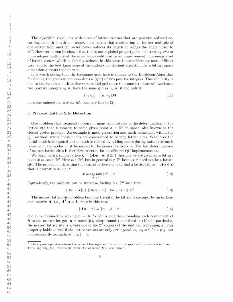
Fig. 2. Example of a point x (square) whose nearest lattice site a2 − a1 is not a corner of the unit cell(vectors and dotted lines).

−1 −0.5 0 0.5 1 1.5 2 2.5 3 3.5−0.5

0

0.5

1

a1

a2

r ≈ 0.604

r ≈ 0.515

x

For non-orthogonal lattice vectors, a1, . . . , ad, this is in general no longer true as canbe seen from the following example, see also Figure 2. Let

A =

1 2

0 1

, x =

1.25

0.55

, n =

0.15

0.55

. (15)

The four corners m = [ 00 ], [ 0

1 ], [ 10 ], and [ 1

1 ] of the unit cell containing x satisfy ‖Am −x‖ > 0.60415, but the nearest lattice site, An = [ 1

1 ] with n = [−11 ], has ‖An − x‖ ≈

0.51479. Thus, the nearest lattice site is not a corner of the unit cell containing x, andn cannot be determined simply by rounding.

Note however that the matrix A from (15) can be reduced to an orthogonal matrix bythe lattice reduction techniques discussed in Section 2, which makes the nearest latticesite detection trivial for this particular example. This does not hold for lattices generatedby arbitrary matrices A, but hints that reducing A to some matrix that is as orthogonalas possible can significantly reduce the computational complexity. Later in this section,we numerically compare the performance of lattice site detection for unmodified, pairwisereduced, and LLL-reduced lattice vector matrices A.

Let us note that for dimension d = 2, it can be proved that the nearest lattice siteis always one of the four corners of the surrounding unit cell if the matrix A is length-reduced. In this case, no further strategy beyond length-reducing the matrix and thenchecking which one of the four corners is nearest is necessary. For higher dimension d ≥ 3,this is no longer true, and other strategies become necessary.

3.1. Brute-Force Method

Given any matrix A, either reduced in some sense or not, the naive brute-force ap-proach to determine the nearest lattice site is to compute the distances to all lattice sitesin the vicinity of x and to take the minimal one. This vicinity needs to be large enoughto ensure that the nearest lattice site is not missed, but should be as small as possiblefor computational efficiency.

In practice, one identifies a corner of the unit cell that contains x, round(n) =round(A−1x), and then scans a rectangular set of indices n around this corner, i.e.,all n with

|ni − round(ni)| ≤ Rb(A) (16)

7

1 2 3 4 5 6 7 8 9 10 11 12 13 14 15 16 17 18 19 20 21 22 23 24 25 26 27 28 29 30 31 32 33 34 35 36 37 38 39 40 41 42 43 44 45 46 47 48 49 50 51 52 53 54 55 56 57 58 59 60 61 62 63 64 65

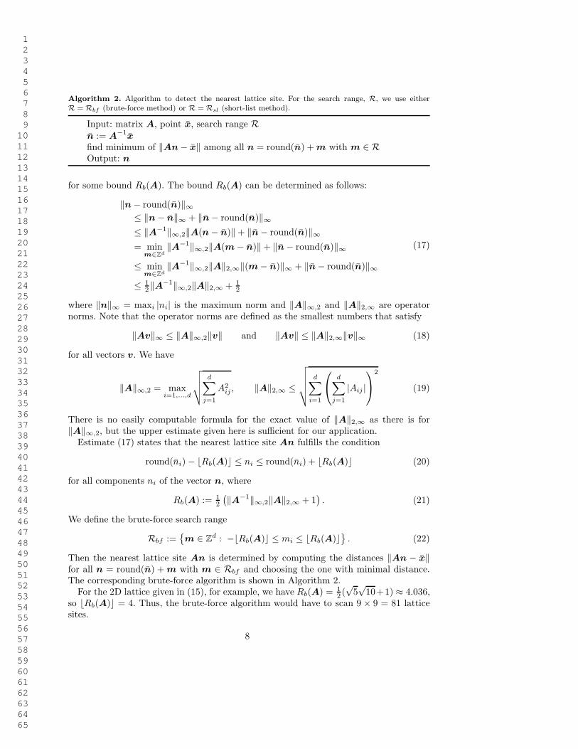
Algorithm 2. Algorithm to detect the nearest lattice site. For the search range, R, we use eitherR = Rbf (brute-force method) or R = Rsl (short-list method).

Input: matrix A, point x, search range Rn := A−1x

find minimum of ‖An − x‖ among all n = round(n) + m with m ∈ ROutput: n

for some bound Rb(A). The bound Rb(A) can be determined as follows:

‖n − round(n)‖∞≤ ‖n − n‖∞ + ‖n − round(n)‖∞≤ ‖A−1‖∞,2‖A(n − n)‖ + ‖n − round(n)‖∞= min

m∈Zd

‖A−1‖∞,2‖A(m − n)‖ + ‖n − round(n)‖∞≤ min

m∈Zd

‖A−1‖∞,2‖A‖2,∞‖(m − n)‖∞ + ‖n − round(n)‖∞≤ 1

2‖A−1‖∞,2‖A‖2,∞ + 1

2

(17)

where ‖n‖∞ = maxi |ni| is the maximum norm and ‖A‖∞,2 and ‖A‖2,∞ are operatornorms. Note that the operator norms are defined as the smallest numbers that satisfy

‖Av‖∞ ≤ ‖A‖∞,2‖v‖ and ‖Av‖ ≤ ‖A‖2,∞‖v‖∞ (18)

for all vectors v. We have

‖A‖∞,2 = maxi=1,...,d

√

√

√

√

d∑

j=1

A2ij , ‖A‖2,∞ ≤

√

√

√

√

√

d∑

i=1

d∑

j=1

|Aij |

2

(19)

There is no easily computable formula for the exact value of ‖A‖2,∞ as there is for‖A‖∞,2, but the upper estimate given here is sufficient for our application.

Estimate (17) states that the nearest lattice site An fulfills the condition

round(ni) − ⌊Rb(A)⌋ ≤ ni ≤ round(ni) + ⌊Rb(A)⌋ (20)

for all components ni of the vector n, where

Rb(A) := 12

(

‖A−1‖∞,2‖A‖2,∞ + 1)

. (21)

We define the brute-force search range

Rbf :=

m ∈ Zd : −⌊Rb(A)⌋ ≤ mi ≤ ⌊Rb(A)⌋

. (22)

Then the nearest lattice site An is determined by computing the distances ‖An − x‖for all n = round(n) + m with m ∈ Rbf and choosing the one with minimal distance.The corresponding brute-force algorithm is shown in Algorithm 2.

For the 2D lattice given in (15), for example, we have Rb(A) = 12 (√

5√

10+1) ≈ 4.036,so ⌊Rb(A)⌋ = 4. Thus, the brute-force algorithm would have to scan 9 × 9 = 81 latticesites.

8

1 2 3 4 5 6 7 8 9 10 11 12 13 14 15 16 17 18 19 20 21 22 23 24 25 26 27 28 29 30 31 32 33 34 35 36 37 38 39 40 41 42 43 44 45 46 47 48 49 50 51 52 53 54 55 56 57 58 59 60 61 62 63 64 65

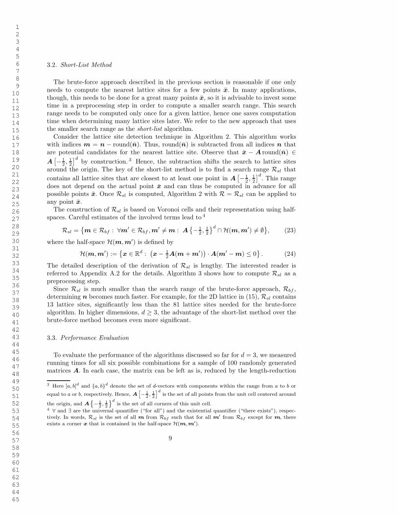
3.2. Short-List Method

The brute-force approach described in the previous section is reasonable if one onlyneeds to compute the nearest lattice sites for a few points x. In many applications,though, this needs to be done for a great many points x, so it is advisable to invest sometime in a preprocessing step in order to compute a smaller search range. This searchrange needs to be computed only once for a given lattice, hence one saves computationtime when determining many lattice sites later. We refer to the new approach that usesthe smaller search range as the short-list algorithm.

Consider the lattice site detection technique in Algorithm 2. This algorithm workswith indices m = n − round(n). Thus, round(n) is subtracted from all indices n thatare potential candidates for the nearest lattice site. Observe that x − A round(n) ∈A

[

− 12 , 1

2

]dby construction. 3 Hence, the subtraction shifts the search to lattice sites

around the origin. The key of the short-list method is to find a search range Rsl that

contains all lattice sites that are closest to at least one point in A[

− 12 , 1

2

]d. This range

does not depend on the actual point x and can thus be computed in advance for allpossible points x. Once Rsl is computed, Algorithm 2 with R = Rsl can be applied toany point x.

The construction of Rsl is based on Voronoi cells and their representation using half-spaces. Careful estimates of the involved terms lead to 4

Rsl =

m ∈ Rbf : ∀m′ ∈ Rbf , m′ 6= m : A

− 12 , 1

2

d ∩H(m, m′) 6= ∅

, (23)

where the half-space H(m, m′) is defined by

H(m, m′) :=

x ∈ Rd :

(

x − 12A(m + m′)

)

· A(m′ − m) ≤ 0

. (24)

The detailed description of the derivation of Rsl is lengthy. The interested reader isreferred to Appendix A.2 for the details. Algorithm 3 shows how to compute Rsl as apreprocessing step.

Since Rsl is much smaller than the search range of the brute-force approach, Rbf ,determining n becomes much faster. For example, for the 2D lattice in (15), Rsl contains13 lattice sites, significantly less than the 81 lattice sites needed for the brute-forcealgorithm. In higher dimensions, d ≥ 3, the advantage of the short-list method over thebrute-force method becomes even more significant.

3.3. Performance Evaluation

To evaluate the performance of the algorithms discussed so far for d = 3, we measuredrunning times for all six possible combinations for a sample of 100 randomly generatedmatrices A. In each case, the matrix can be left as is, reduced by the length-reduction

3 Here [a, b]d and a, bd denote the set of d-vectors with components within the range from a to b or

equal to a or b, respectively. Hence, A

[

− 1

2, 1

2

]dis the set of all points from the unit cell centered around

the origin, and A

− 1

2, 1

2

dis the set of all corners of this unit cell.

4 ∀ and ∃ are the universal quantifier (“for all”) and the existential quantifier (“there exists”), respec-tively. In words, Rsl is the set of all m from Rbf such that for all m′ from Rbf except for m, thereexists a corner x that is contained in the half-space H(m, m′).

9

1 2 3 4 5 6 7 8 9 10 11 12 13 14 15 16 17 18 19 20 21 22 23 24 25 26 27 28 29 30 31 32 33 34 35 36 37 38 39 40 41 42 43 44 45 46 47 48 49 50 51 52 53 54 55 56 57 58 59 60 61 62 63 64 65

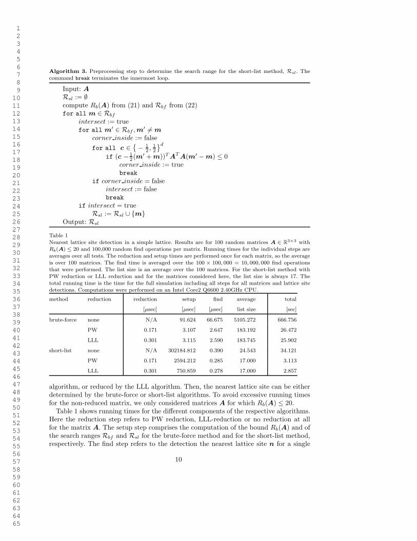
Algorithm 3. Preprocessing step to determine the search range for the short-list method, Rsl. Thecommand break terminates the innermost loop.

Input: A

Rsl := ∅compute Rb(A) from (21) and Rbf from (22)for all m ∈ Rbf

intersect := truefor all m′ ∈ Rbf , m′ 6= m

corner inside := false

for all c ∈

− 12 , 1

2

d

if (c − 12 (m′ + m))T AT A(m′ − m) ≤ 0

corner inside := truebreak

if corner inside = falseintersect := falsebreak

if intersect = trueRsl := Rsl ∪ m

Output: Rsl

Table 1Nearest lattice site detection in a simple lattice. Results are for 100 random matrices A ∈ R

3×3 withRb(A) ≤ 20 and 100,000 random find operations per matrix. Running times for the individual steps areaverages over all tests. The reduction and setup times are performed once for each matrix, so the averageis over 100 matrices. The find time is averaged over the 100 × 100, 000 = 10, 000, 000 find operationsthat were performed. The list size is an average over the 100 matrices. For the short-list method withPW reduction or LLL reduction and for the matrices considered here, the list size is always 17. Thetotal running time is the time for the full simulation including all steps for all matrices and lattice sitedetections. Computations were performed on an Intel Core2 Q6600 2.40GHz CPU.

method reduction reduction setup find average total

[µsec] [µsec] [µsec] list size [sec]

brute-force none N/A 91.624 66.675 5105.272 666.756

PW 0.171 3.107 2.647 183.192 26.472

LLL 0.301 3.115 2.590 183.745 25.902

short-list none N/A 302184.812 0.390 24.543 34.121

PW 0.171 2594.212 0.285 17.000 3.113

LLL 0.301 750.859 0.278 17.000 2.857

algorithm, or reduced by the LLL algorithm. Then, the nearest lattice site can be eitherdetermined by the brute-force or short-list algorithms. To avoid excessive running timesfor the non-reduced matrix, we only considered matrices A for which Rb(A) ≤ 20.

Table 1 shows running times for the different components of the respective algorithms.Here the reduction step refers to PW reduction, LLL-reduction or no reduction at allfor the matrix A. The setup step comprises the computation of the bound Rb(A) and ofthe search ranges Rbf and Rsl for the brute-force method and for the short-list method,respectively. The find step refers to the detection the nearest lattice site n for a single

10

1 2 3 4 5 6 7 8 9 10 11 12 13 14 15 16 17 18 19 20 21 22 23 24 25 26 27 28 29 30 31 32 33 34 35 36 37 38 39 40 41 42 43 44 45 46 47 48 49 50 51 52 53 54 55 56 57 58 59 60 61 62 63 64 65

point x. The results show that the reduction step, either PW or LLL, costs nearly nocomputation time, but that it greatly reduces the time for the subsequent setup and findoperations. Bearing in mind that the reduction step just needs to be done once for eachmatrix, it is a clear must. The setup phase of the short-list method costs additional timecompared to the brute-force method because it scales as Rb(A)2d compared to Rb(A)d.However, it accelerates the subsequent find operations by a factor of 9 on average, thusit pays off if many find operations are performed. Based on Table 1, the actual crossoverpoint for which the short-list algorithm is favorable to the brute-force algorithm is 1098find operations if PW-reduction is used and 324 find operations if LLL-reduction isused. The lattice-reduced approaches also have significant storage advantages over thecorresponding unreduced approaches as shown by the list size requirements (i.e., theaverage number of lattice sites scanned during a find operation).

Table 1 also shows the total running time for a practical application consisting of100 different matrices A ∈ R

3×3 with 100,000 find operations each. Clearly the short-list method for the reduced matrices is best, with LLL slightly faster than PW. Theadvantage of the PW approach is that it has a clear geometric significance and is muchsimpler to implement than LLL, while being nearly as efficient. The brute-force methodsand the non-reduced methods are not competitive.

An important variation of the nearest lattice site detection problem is the restriction toa finite-sized domain, Ω ⊂ R

d. Consider the problem of seeking the lattice site from L∩Ωthat is nearest to x ∈ Ω. If x is far from the boundary ∂Ω of the domain, the problemdoes not differ from finding the nearest lattice site from the full lattice L. However, closeto the boundary, the nearest site from L∩Ω might not be the nearest site from L, and thecarefully constructed search list for the original problem might miss the correct latticesite. It is therefore advisable to proceed as follows. First, the nearest lattice site from thefull lattice L is determined using the short-list algorithm. If this lattice site lies withinthe domain Ω, we have found the solution. Otherwise, we fall back to searching from amuch larger set, such as the one used in the brute-force method. It is important to note,though, that the correct result is not guaranteed even for the brute-force method if thedomain Ω is highly irregular. In the worst case, any site from L ∩ Ω could be nearest.In practice, it will not be necessary to revert to the slow brute-force approach in mostcases, hence we still have a quite efficient method.

3.4. Nearest Lattice Site Detection for Multilattices

Up to now, we discussed how to detect the nearest lattice site within a simple latticeas given by (1). We now extend this to multilattices.

A multilattice is a set of S inter-penetrating simple lattices called sublattices. 5 The setof lattice sites making up the multilattice is

L = A(n + να) : n ∈ Zd, α = 1, . . . , S, (25)

5 It is also possible to think of a multilattice structure as a simple lattice with more than one pointassociated with each lattice site. This interpretation has led to the term lattice with a basis, which iscommon in the physics literature. In this context, the set of “points” located at each lattice site is calledthe basis. For a crystal structure, the basis corresponds to a set of atoms. If a single atom is placed ateach lattice site, the result is a simple crystal structure. If the basis contains multiple atoms, the resultis a complex or multilattice crystal.

11

1 2 3 4 5 6 7 8 9 10 11 12 13 14 15 16 17 18 19 20 21 22 23 24 25 26 27 28 29 30 31 32 33 34 35 36 37 38 39 40 41 42 43 44 45 46 47 48 49 50 51 52 53 54 55 56 57 58 59 60 61 62 63 64 65

where 3 να ∈ [0, 1)d (α = 1, . . . , S) are the positions of the sublattices (also called frac-

tional position vectors) relative to the nominal simple lattice that serves as the scaffoldingfor the multilattice (sometimes called the “skeletal lattice”). We say that each nominallattice site has S sublattice sites associated with it. Clearly, if S = 1, the multilatticereduces to a simple lattice, possibly shifted relative to the nominal lattice.

When applying the nearest lattice site algorithm to the multilattice in (25), it is neces-sary to account for the fractional position vectors να. The objective is to find the latticesite A(n + να) satisfying

‖A(n + να) − x‖ ≤ ‖A(m + νβ) − x‖ for all m ∈ Zd, β = 1, . . . , S. (26)

Compare this condition to (13). Obviously

A(n + να) − x = An − (x − Aνα). (27)

Thus, for a single position vector (S = 1), the problem reduces to the case of a simple lat-tice where the point x is replaced by x−Aν1. For a multilattice with several sublattices,we apply one of the techniques for simple lattices discussed earlier to each position vectorνα, individually. In this manner, we obtain lattice sites A(nα + να) that are nearest tox among the shifted simple lattice Am + να : m ∈ Z

d. The overall solution to (26) isthen obtained by choosing the lattice site A(nα + να) with the minimal distance to x

among all the sublattices α = 1, . . . , S.Note that we have not addressed the important issue of essential versus non-essential

descriptions of multilattices [10]. The essential description is the multilattice with theminimal value of S that reproduces the lattice structure. Of course, it is always possibleto represent a simple lattice or a multilattice with S sublattices by another multilatticewith larger periodicity and correspondingly larger S. This is a non-essential description.The algorithms given above will work for non-essential descriptions, but would be accel-erated by using the essential representation. The problem of determining the essentialdescription for a given multilattice is an important problem that lies outside the scopeof this paper. See for example [9] for a discussion of this issue.

4. Cluster Construction

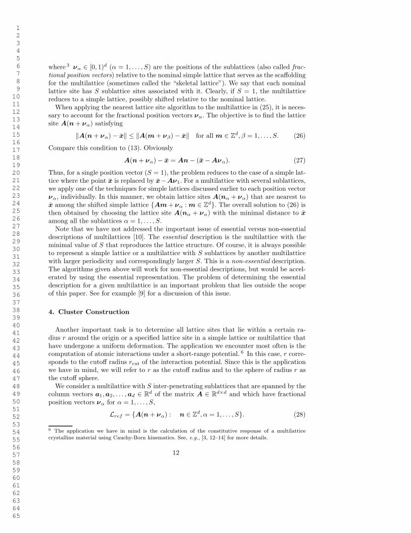
Another important task is to determine all lattice sites that lie within a certain ra-dius r around the origin or a specified lattice site in a simple lattice or multilattice thathave undergone a uniform deformation. The application we encounter most often is thecomputation of atomic interactions under a short-range potential. 6 In this case, r corre-sponds to the cutoff radius rcut of the interaction potential. Since this is the applicationwe have in mind, we will refer to r as the cutoff radius and to the sphere of radius r asthe cutoff sphere.

We consider a multilattice with S inter-penetrating sublattices that are spanned by thecolumn vectors a1, a2, . . . , ad ∈ R

d of the matrix A ∈ Rd×d and which have fractional

position vectors να for α = 1, . . . , S,

Lref = A(n + να) : n ∈ Zd, α = 1, . . . , S. (28)

6 The application we have in mind is the calculation of the constitutive response of a multilatticecrystalline material using Cauchy-Born kinematics. See, e.g., [3, 12–14] for more details.

12

1 2 3 4 5 6 7 8 9 10 11 12 13 14 15 16 17 18 19 20 21 22 23 24 25 26 27 28 29 30 31 32 33 34 35 36 37 38 39 40 41 42 43 44 45 46 47 48 49 50 51 52 53 54 55 56 57 58 59 60 61 62 63 64 65

The lattice Lref is referred to as the reference configuration. The sublattices undergo auniform deformation described by the affine mapping y(x) = Fx+uα, where F ∈ R

d×d isa regular matrix and where uα ∈ R

d are shift vectors that displace the sublattices relativeto each other. In continuum mechanics applications, F is the deformation gradient, whichis how we will refer to it here. The deformed configuration L of the multilattice followsfrom (28) as

L = FA(n + να) + uα : n ∈ Zd, α = 1, . . . , S

= FA(n + sα) : n ∈ Zd, α = 1, . . . , S

= FAn + δα : n ∈ Zd, α = 1, . . . , S,

(29)

where sα = να +A−1F−1uα and where we refer to δα = FAνα +uα as the offset vector

of sublattice α.Two problems are of interest in this context. The first problem is to find all lattice

sites (n, α) satisfying

‖FA(n + sα)‖ ≤ r, (30)

i.e., all lattice sites within distance r of the origin. The second problem is to find alllattice sites (n, α) that are within distance r of a given lattice site (n, α),

‖FA(n + sα) − FA(n + sα)‖ ≤ r. (31)

Due to the translation invariance of the infinite lattice, we may set n = 0 without lossof generality. Thus, the second problem becomes equivalent to the first one with thesublattice positions replaced by their differences. We therefore have the generic problem,

‖FA(n + s)‖ ≤ r, (32)

where s is either sα or sα − sα. Below, we develop two different algorithms to efficientlydetermine all n ∈ Z

d satisfying (32) for given r > 0 and s ∈ Rd. The two problems

described above are then solved by repeatedly applying one of these algorithms to alls = sα with α = 1, . . . , S (first problem) or to all s = sα − sα with α, α = 1, . . . , S(second problem), respectively. We derive the methods for multilattices. The case forsimple lattices follows as a special case by setting S = 1.

4.1. Algorithms for Cluster Construction in Multilattices

In this section, we derive two methods to solve problem (32): the shell algorithm andthe on-the-fly algorithm.

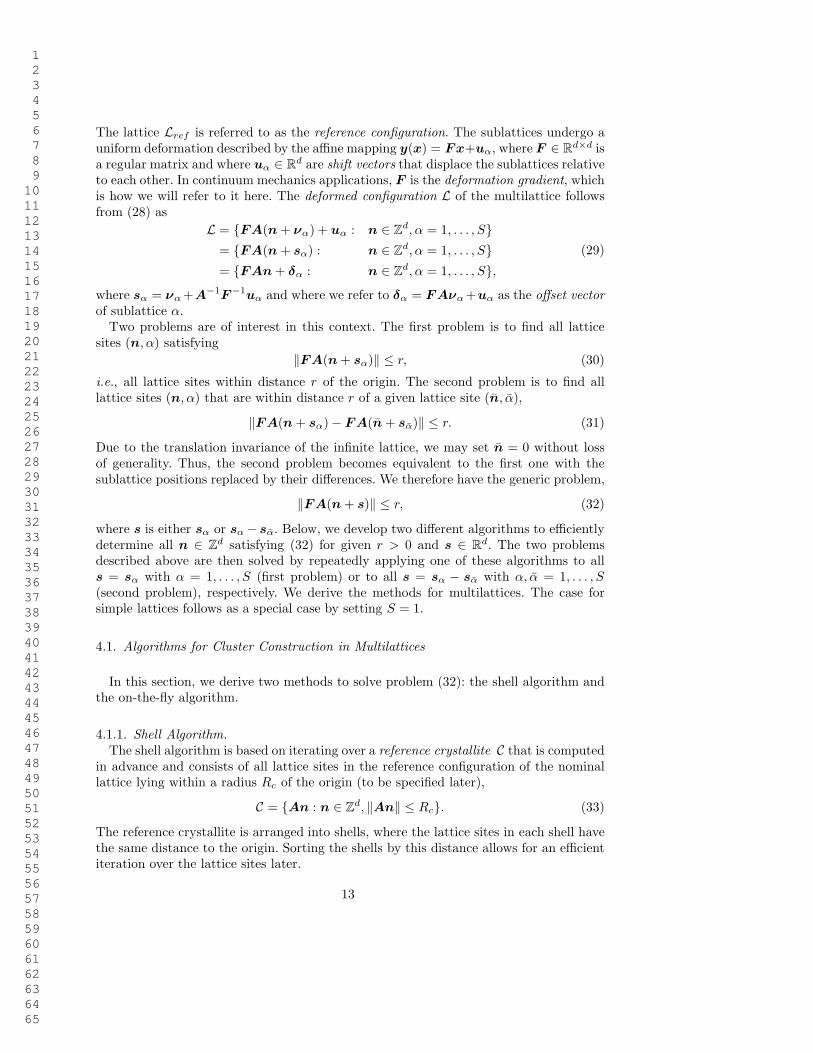
4.1.1. Shell Algorithm.

The shell algorithm is based on iterating over a reference crystallite C that is computedin advance and consists of all lattice sites in the reference configuration of the nominallattice lying within a radius Rc of the origin (to be specified later),

C = An : n ∈ Zd, ‖An‖ ≤ Rc. (33)

The reference crystallite is arranged into shells, where the lattice sites in each shell havethe same distance to the origin. Sorting the shells by this distance allows for an efficientiteration over the lattice sites later.

13

1 2 3 4 5 6 7 8 9 10 11 12 13 14 15 16 17 18 19 20 21 22 23 24 25 26 27 28 29 30 31 32 33 34 35 36 37 38 39 40 41 42 43 44 45 46 47 48 49 50 51 52 53 54 55 56 57 58 59 60 61 62 63 64 65

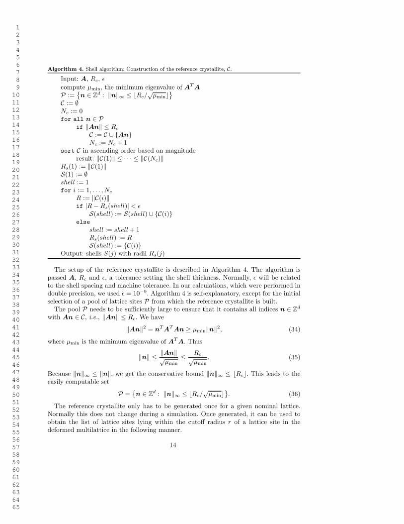
Algorithm 4. Shell algorithm: Construction of the reference crystallite, C.

Input: A, Rc, ǫ

compute µmin, the minimum eigenvalue of AT A

P :=

n ∈ Zd : ‖n‖∞ ≤ ⌊Rc/

√µmin⌋

C := ∅Nc := 0for all n ∈ P

if ‖An‖ ≤ Rc

C := C ∪ AnNc := Nc + 1

sort C in ascending order based on magnituderesult: ‖C(1)‖ ≤ · · · ≤ ‖C(Nc)‖

Rs(1) := ‖C(1)‖S(1) := ∅shell := 1for i := 1, . . . , Nc

R := ‖C(i)‖if |R − Rs(shell)| < ǫ

S(shell) := S(shell) ∪ C(i)else

shell := shell + 1Rs(shell) := RS(shell) := C(i)

Output: shells S(j) with radii Rs(j)

The setup of the reference crystallite is described in Algorithm 4. The algorithm ispassed A, Rc and ǫ, a tolerance setting the shell thickness. Normally, ǫ will be relatedto the shell spacing and machine tolerance. In our calculations, which were performed indouble precision, we used ǫ = 10−9. Algorithm 4 is self-explanatory, except for the initialselection of a pool of lattice sites P from which the reference crystallite is built.

The pool P needs to be sufficiently large to ensure that it contains all indices n ∈ Zd

with An ∈ C, i.e., ‖An‖ ≤ Rc. We have

‖An‖2 = nT AT An ≥ µmin‖n‖2, (34)

where µmin is the minimum eigenvalue of AT A. Thus

‖n‖ ≤ ‖An‖√µmin

≤ Rc√µmin

. (35)

Because ‖n‖∞ ≤ ‖n‖, we get the conservative bound ‖n‖∞ ≤ ⌊Rc⌋. This leads to theeasily computable set

P =

n ∈ Zd : ‖n‖∞ ≤ ⌊Rc/

√µmin⌋

. (36)

The reference crystallite only has to be generated once for a given nominal lattice.Normally this does not change during a simulation. Once generated, it can be used toobtain the list of lattice sites lying within the cutoff radius r of a lattice site in thedeformed multilattice in the following manner.

14

1 2 3 4 5 6 7 8 9 10 11 12 13 14 15 16 17 18 19 20 21 22 23 24 25 26 27 28 29 30 31 32 33 34 35 36 37 38 39 40 41 42 43 44 45 46 47 48 49 50 51 52 53 54 55 56 57 58 59 60 61 62 63 64 65

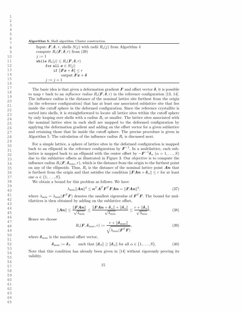
Algorithm 5. Shell algorithm: Cluster construction.

Input: F , δ, r, shells S(j) with radii Rs(j) from Algorithm 4compute Ri(F , δ, r) from (39)j := 1while Rs(j) ≤ Ri(F , δ, r)

for all x ∈ S(j)if ‖Fx + δ‖ ≤ r

output Fx + δ

j := j + 1

The basic idea is that given a deformation gradient F and offset vector δ, it is possibleto map r back to an influence radius Ri(F , δ, r) in the reference configuration [13, 14].The influence radius is the distance of the nominal lattice site furthest from the origin(in the reference configuration) that has at least one associated sublattice site that liesinside the cutoff sphere in the deformed configuration. Since the reference crystallite issorted into shells, it is straightforward to locate all lattice sites within the cutoff sphereby only looping over shells with a radius Ri or smaller. The lattice sites associated withthe nominal lattice sites in each shell are mapped to the deformed configuration byapplying the deformation gradient and adding on the offset vector for a given sublatticeand retaining those that lie inside the cutoff sphere. The precise procedure is given inAlgorithm 5. The calculation of the influence radius Ri is discussed next.

For a simple lattice, a sphere of lattice sites in the deformed configuration is mappedback to an ellipsoid in the reference configuration by F−1. In a multilattice, each sub-lattice is mapped back to an ellipsoid with the center offset by −F−1δα (α = 1, . . . , S)due to the sublattice offsets as illustrated in Figure 3. Our objective is to compute theinfluence radius Ri(F , δmax, r), which is the distance from the origin to the furthest pointon any of the ellipsoids. Thus, Ri is the distance of the nominal lattice point An thatis furthest from the origin and that satisfies the condition ‖FAn + δα‖ ≤ r for at leastone α ∈ 1, . . . , S.

We obtain a bound for this problem as follows. We have

λmin‖An‖2 ≤ nT AT F T FAn = ‖FAn‖2, (37)

where λmin = λmin(FT F ) denotes the smallest eigenvalue of F T F . The bound for mul-

tilattices is then obtained by adding on the sublattice offset,

‖An‖ ≤ ‖FAn‖√λmin

≤ ‖FAn + δα‖ + ‖δα‖√λmin

≤ r + ‖δα‖√λmin

. (38)

Hence we choose

Ri(F , δmax, r) :=r + ‖δmax‖

√

λmin(F T F ), (39)

where δmax is the maximal offset vector,

δmax := δβ such that ‖δβ‖ ≥ ‖δα‖ for all α ∈ 1, . . . , S. (40)

Note that this condition has already been given in [14] without rigorously proving itsvalidity.

15

1 2 3 4 5 6 7 8 9 10 11 12 13 14 15 16 17 18 19 20 21 22 23 24 25 26 27 28 29 30 31 32 33 34 35 36 37 38 39 40 41 42 43 44 45 46 47 48 49 50 51 52 53 54 55 56 57 58 59 60 61 62 63 64 65

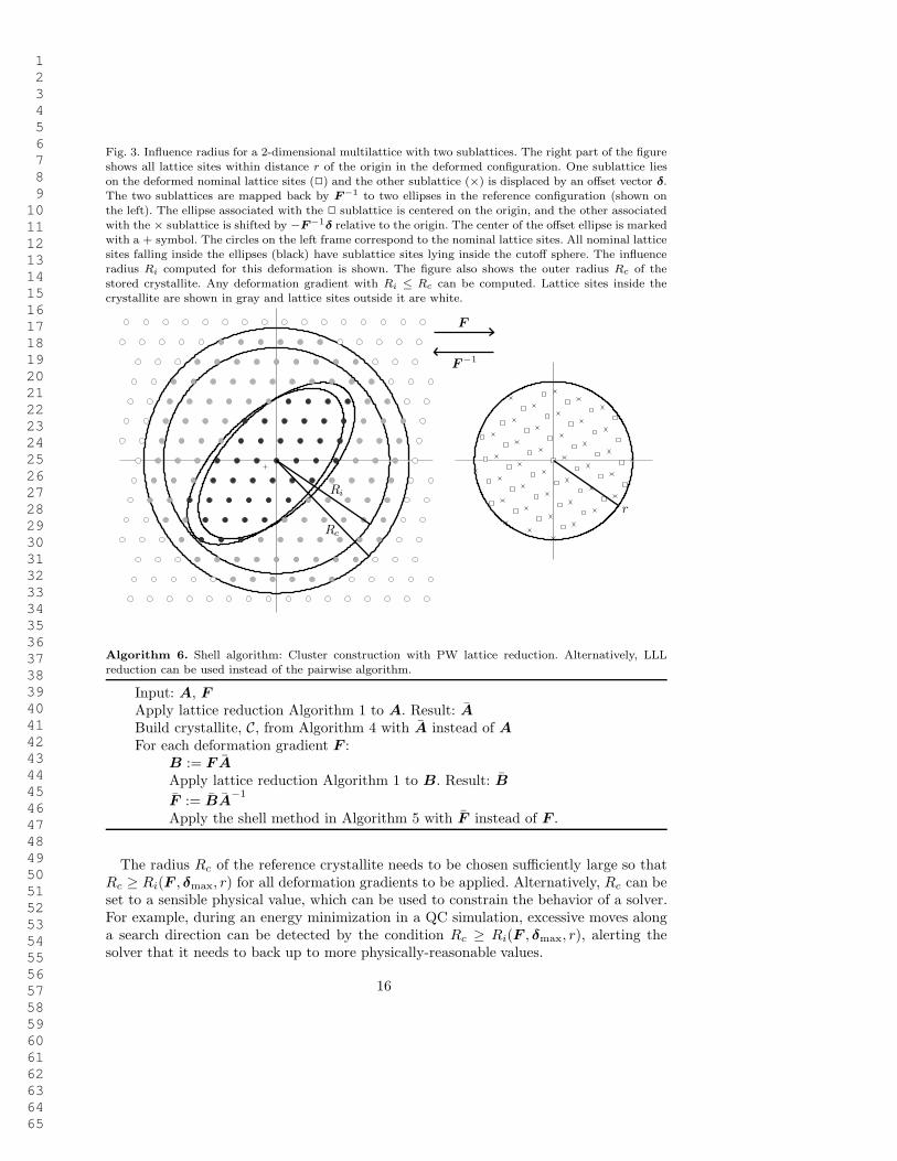
Fig. 3. Influence radius for a 2-dimensional multilattice with two sublattices. The right part of the figureshows all lattice sites within distance r of the origin in the deformed configuration. One sublattice lieson the deformed nominal lattice sites (2) and the other sublattice (×) is displaced by an offset vector δ.The two sublattices are mapped back by F

−1 to two ellipses in the reference configuration (shown onthe left). The ellipse associated with the 2 sublattice is centered on the origin, and the other associatedwith the × sublattice is shifted by −F

−1δ relative to the origin. The center of the offset ellipse is marked

with a + symbol. The circles on the left frame correspond to the nominal lattice sites. All nominal latticesites falling inside the ellipses (black) have sublattice sites lying inside the cutoff sphere. The influenceradius Ri computed for this deformation is shown. The figure also shows the outer radius Rc of thestored crystallite. Any deformation gradient with Ri ≤ Rc can be computed. Lattice sites inside thecrystallite are shown in gray and lattice sites outside it are white.

Ri

Rc

r

F

F−1

Algorithm 6. Shell algorithm: Cluster construction with PW lattice reduction. Alternatively, LLLreduction can be used instead of the pairwise algorithm.

Input: A, F

Apply lattice reduction Algorithm 1 to A. Result: A

Build crystallite, C, from Algorithm 4 with A instead of A

For each deformation gradient F :B := FA

Apply lattice reduction Algorithm 1 to B. Result: B

F := BA−1

Apply the shell method in Algorithm 5 with F instead of F .

The radius Rc of the reference crystallite needs to be chosen sufficiently large so thatRc ≥ Ri(F , δmax, r) for all deformation gradients to be applied. Alternatively, Rc can beset to a sensible physical value, which can be used to constrain the behavior of a solver.For example, during an energy minimization in a QC simulation, excessive moves alonga search direction can be detected by the condition Rc ≥ Ri(F , δmax, r), alerting thesolver that it needs to back up to more physically-reasonable values.

16

1 2 3 4 5 6 7 8 9 10 11 12 13 14 15 16 17 18 19 20 21 22 23 24 25 26 27 28 29 30 31 32 33 34 35 36 37 38 39 40 41 42 43 44 45 46 47 48 49 50 51 52 53 54 55 56 57 58 59 60 61 62 63 64 65

The shell method can often be accelerated by applying a lattice reduction procedureto obtain a “smaller” deformation gradient by factoring out the lattice invariant portionof the deformation. 7 The procedure involves a setup stage that has to be done once andan application stage, which is repeated for each deformation gradient.

The setup stage involves the following steps. First, PW or LLL lattice reduction isapplied to the reference lattice vectors in matrix A. This results in an optimized referencelattice given by A. 8 Recall that the reference lattice spanned by A is the same as thelattice spanned by A, only the corresponding indices n may differ. Second, the crystalliteC is computed with Algorithm 4, where A is replaced by A. This completes the setupstage.

The application stage involves the following steps. For every deformation gradientF , the deformed lattice B = FA is lattice reduced to B. The corresponding reduceddeformation gradient F follows from the requirement B = F A, thus

F = BA−1

. (41)

The shell method in Algorithm 5 is then applied using F instead of the original defor-mation gradient F . The approach is outlined in Algorithm 6 with PW lattice reduction.Of course, LLL lattice reduction could be used instead.

The saving in computational time as a result of this algorithm can be significant. Forexample, if a lattice invariant shear is applied to the system, i.e., a shear that leavesthe lattice unchanged, then B = A and therefore F = I, which is an optimal case forthe shell method. Timing studies for this example are given in Sections 4.2 and 4.3 for asimple lattice and multilattices.

4.1.2. On-the-Fly Algorithm.

The second technique is to determine the lattice sites entirely in the deformed configu-ration. We refer to this method as the on-the-fly (OTF) algorithm. Rather than loopingover lattice sites in the reference configuration and mapping them to the deformed con-figuration, the lattice vectors themselves are mapped to the deformed configuration, FA,and the lattice sites lying within the cutoff sphere are determined on-the-fly by means ofd nested loops with certain bounds. The bounds are chosen carefully to exactly give thecorrect set of lattice sites, at the cost of some computational overhead to compute thesebounds.

LetG := AT F T FA ∈ R

d×d. (42)

Note that G is symmetric positive definite, provided that both A and F are regular.Then our problem is to identify all n ∈ Z

d with

(n + s)T G(n + s) ≤ r2. (43)

To isolate the last component nd of n, we subdivide G, n, and s into blocks as

G =

G g

gT γ

, n =

n

nd

, s =

s

sd

(44)

7 A lattice invariant deformation is one that leaves an infinite lattice unchanged.8 The lattice vectors given in textbooks for physically-relevant crystal structures are normally alreadyreduced. In this case the lattice reduction step would simply return A = A.

17

1 2 3 4 5 6 7 8 9 10 11 12 13 14 15 16 17 18 19 20 21 22 23 24 25 26 27 28 29 30 31 32 33 34 35 36 37 38 39 40 41 42 43 44 45 46 47 48 49 50 51 52 53 54 55 56 57 58 59 60 61 62 63 64 65

with G ∈ R(d−1)×(d−1), g ∈ R

d−1, γ ∈ R, n ∈ Zd−1, nd ∈ Z, s ∈ R

d−1, and sd ∈ R.Using this notation, (43) reads as

(n + s)T G(n + s) + 2(nd + sd)gT (n + s) + γ(nd + sd)

2 ≤ r2, (45)

or equivalently

(√γnd +

gT (n + s) + γsd√γ

)2

≤ r2 − (n + s)T G(n + s) (46)

with

G := G − g ⊗ g

γ, (47)

where g ⊗ g is the self dyad of g, which in component form is (g ⊗ g)ij = gigj .If we treat n as known for now, we obtain the condition

− gT (n + s) + γsd

γ−

√

r2 − (n + s)T G(n + s)

γ

≤ nd ≤− gT (n + s) + γsd

γ+

√

r2 − (n + s)T G(n + s)

γ

(48)

for the remaining coordinate nd. This inequality gives the bounds for the innermost loopover nd.

After having separated the component nd, we now turn to nd−1. Observe that (46)can only hold if its right-hand side is non-negative, i.e.,

(n + s)T G(n + s) ≤ r2. (49)

Just as G, the matrix G is symmetric positive definite as well, see Lemma A.3 in theappendix. Hence condition (49) has the same structure as (43) where the dimensions ofthe vectors and matrices are d − 1 instead of d and (d − 1) × (d − 1) instead of d × d,respectively. Thus, the same strategy that was used for G ∈ R

d×d and n ∈ Zd can be

used for G ∈ R(d−1)×(d−1) and n ∈ Z

d−1 to get the second innermost loop over nd−1.This process is continued until we get the outermost loop over n1.

The whole procedure is shown in Algorithm 7. Note that the ranges given for thematrices G(i) correspond to the submatrices G, g and γ used in the text. This hasbeen done to emphasize that it is not necessary to actually declare variables for thesubmatrices, instead it is sufficient and usually faster to just access the correspondingpart of G(i). The same holds for n and s.

A minor possible improvement that we do not consider here is the effect of the coordi-nate system orientation and the ordering of the loops in Algorithm 7 on the performanceof the OTF method. The method would be most efficient if the number of bounds calcu-lations were minimized. This is achieved if outer loops correspond to spatial directionsfor which the bounds are closer together. Clearly,

for i := 0, . . . , 2; for j := 0, . . . , 10; . . . (50)

is more efficient than

for j := 0, . . . , 10; for i := 0, . . . , 2; . . . (51)

18

1 2 3 4 5 6 7 8 9 10 11 12 13 14 15 16 17 18 19 20 21 22 23 24 25 26 27 28 29 30 31 32 33 34 35 36 37 38 39 40 41 42 43 44 45 46 47 48 49 50 51 52 53 54 55 56 57 58 59 60 61 62 63 64 65

Algorithm 7. On-the-fly algorithm: cluster construction.

Input: A, F , s, r

G(d) := AT F T FA

for i := d, . . . , 2

G(i−1) := G(i)1...i−1,1...i−1 − G

(i)1...i−1,iG

(i)i,1...i−1/G

(i)i,i

α1 := s1

β1 :=√

r2/G(1)1,1

for n1 := ⌈−α1 − β1⌉, . . . , ⌊−α1 + β1⌋. . .

αi := G(i)i,1...i−1(n + s)1...i−1/G

(i)i,i + si

βi :=

√

(

r2 − (n + s)T1...i−1G

(i−1)(n + s)1...i−1

)

/G(i)i,i

for ni := ⌈−αi − βi⌉, . . . , ⌊−αi + βi⌋. . .

αd := G(d)d,1...d−1(n + s)1...d−1/G

(d)d,d + sd

βd :=

√

(

r2 − (n + s)T1...d−1G

(d−1)(n + s)1...d−1

)

/G(d)d,d

for nd := ⌈−αd − βd⌉, . . . , ⌊−αd + βd⌋output n

assuming that the bounds of the inner loop have to be computed each time. The optimaldirections can be determined by computing the principle directions of the deformation.However the cost of doing so would probably offset any gains and was not done here.

4.2. Timing Results for Simple Lattices

In this section timing results for simple lattices are presented to assess the efficiencyof the methods discussed above: the shell method (S) given in Algorithm 5, the shellmethod with PW-lattice reduction (S+PW) given in Algorithm 6, and the OTF methodgiven in Algorithm 7. The reference configuration for the calculations shown here is athree-dimensional simple cubic lattice with a normalized lattice parameter a = 1, so that

A =

1 0 0

0 1 0

0 0 1

. (52)

To explore the dependence of the methods on the cutoff radius r, three different radiiare tested: r = 1.0, 1.732, 3.126, corresponding to a 1st (1-NN), 3rd (3-NN), 9th (9-NN)neighbor model. 9 The models contain respectively 7, 27, 147 lattice sites in the referenceconfiguration (including the lattice site at the origin). The normalized reference crystalliteradius used in the shell method S is set to be Rc = 20, selected to be large enough forall investigated deformations.

9 By an nth-neighbor model, we mean a choice of cutoff radius that in the reference configurationcontains all lattice sites up to and including the nth nearest neighbor shell of lattice sites to the origin.

19

1 2 3 4 5 6 7 8 9 10 11 12 13 14 15 16 17 18 19 20 21 22 23 24 25 26 27 28 29 30 31 32 33 34 35 36 37 38 39 40 41 42 43 44 45 46 47 48 49 50 51 52 53 54 55 56 57 58 59 60 61 62 63 64 65

In our timing analysis two types of deformations with deformation gradient F areapplied to the reference configuration: simple shear and uniaxial stretch. This choice ismotivated by the QR decomposition theorem, see, e.g., [11]. According to this theorem,any matrix F can be factorized as F = QR, where the first factor, Q, is an orthog-onal matrix corresponding to rotation and reflection, and the second factor, R, is anupper triangular matrix. Furthermore, the upper triangular matrix, R, can be writtenas a product R = DS of a diagonal matrix, D, representing a stretch deformation,and an upper triangular matrix with unit diagonal, S, representing a shear deformation.Rotations and reflections do not change the actual structure of the lattice. Thus, shearand stretch deformations are two prototypical deformations from which all other defor-mations can be constructed. The deformation gradients for simple shear and uniaxialstretch along the x-direction are given by

F =

1 γ 0

0 1 0

0 0 1

and F =

λ 0 0

0 1 0

0 0 1

, (53)

respectively. Here γ and λ are the dimensionless shear and stretch parameters that setthe magnitude of the deformation.

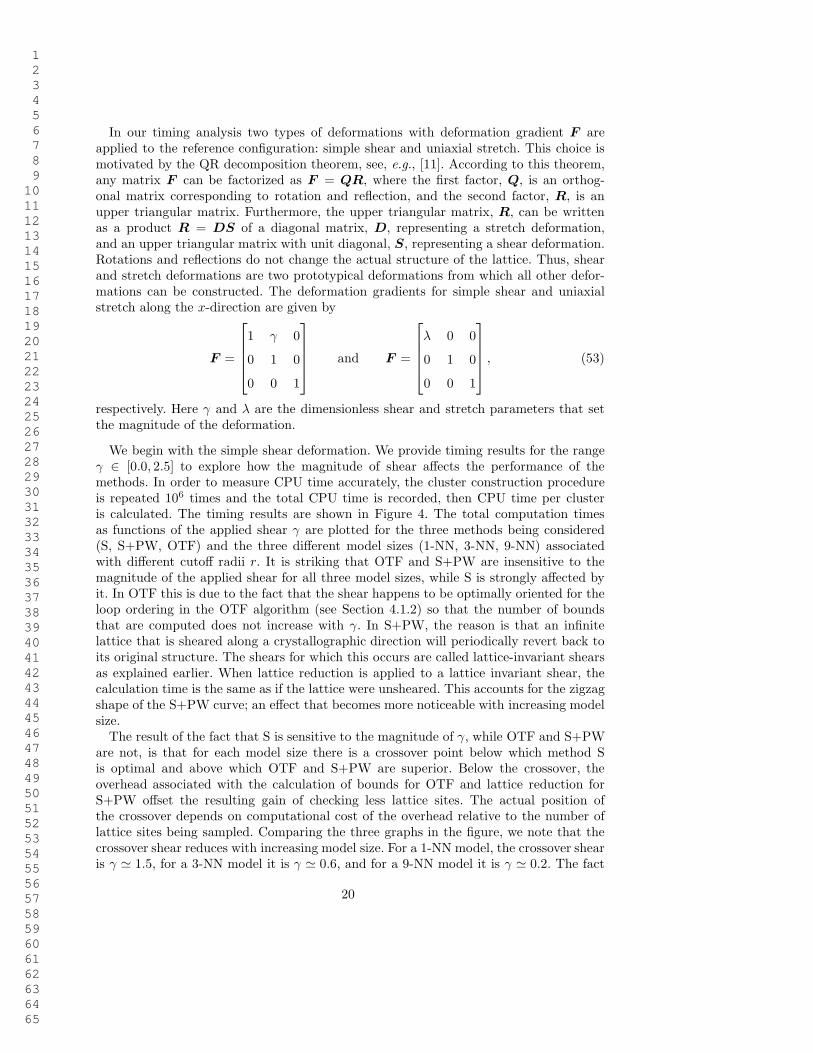
We begin with the simple shear deformation. We provide timing results for the rangeγ ∈ [0.0, 2.5] to explore how the magnitude of shear affects the performance of themethods. In order to measure CPU time accurately, the cluster construction procedureis repeated 106 times and the total CPU time is recorded, then CPU time per clusteris calculated. The timing results are shown in Figure 4. The total computation timesas functions of the applied shear γ are plotted for the three methods being considered(S, S+PW, OTF) and the three different model sizes (1-NN, 3-NN, 9-NN) associatedwith different cutoff radii r. It is striking that OTF and S+PW are insensitive to themagnitude of the applied shear for all three model sizes, while S is strongly affected byit. In OTF this is due to the fact that the shear happens to be optimally oriented for theloop ordering in the OTF algorithm (see Section 4.1.2) so that the number of boundsthat are computed does not increase with γ. In S+PW, the reason is that an infinitelattice that is sheared along a crystallographic direction will periodically revert back toits original structure. The shears for which this occurs are called lattice-invariant shearsas explained earlier. When lattice reduction is applied to a lattice invariant shear, thecalculation time is the same as if the lattice were unsheared. This accounts for the zigzagshape of the S+PW curve; an effect that becomes more noticeable with increasing modelsize.

The result of the fact that S is sensitive to the magnitude of γ, while OTF and S+PWare not, is that for each model size there is a crossover point below which method Sis optimal and above which OTF and S+PW are superior. Below the crossover, theoverhead associated with the calculation of bounds for OTF and lattice reduction forS+PW offset the resulting gain of checking less lattice sites. The actual position ofthe crossover depends on computational cost of the overhead relative to the number oflattice sites being sampled. Comparing the three graphs in the figure, we note that thecrossover shear reduces with increasing model size. For a 1-NN model, the crossover shearis γ ≃ 1.5, for a 3-NN model it is γ ≃ 0.6, and for a 9-NN model it is γ ≃ 0.2. The fact

20

1 2 3 4 5 6 7 8 9 10 11 12 13 14 15 16 17 18 19 20 21 22 23 24 25 26 27 28 29 30 31 32 33 34 35 36 37 38 39 40 41 42 43 44 45 46 47 48 49 50 51 52 53 54 55 56 57 58 59 60 61 62 63 64 65

Fig. 4. Cluster construction in simple lattices undergoing simple shear. The time required to find alllattice sites within a given cutoff radius of the origin as a function of the applied shear γ. Three differentradii are considered corresponding to a nearest-neighbor mode (1-NN), third-neighbor model (3-NN),and ninth-neighbor model (9-NN).

0 0.5 1 1.5 2 2.5γ

0

0.2

0.4

0.6

0.8

1

1.2

CPU

tim

e (µ

sec)

OTFSS+PW

1-NN

0 0.5 1 1.5 2 2.5γ

0

1

2

3

4

5

6

CPU

tim

e (µ

sec)

OTFS+PWS

3-NN

0 0.5 1 1.5 2 2.5γ

0

10

20

30

40

CPU

tim

e (µ

sec)

OTFSS+PW

9-NN

21

1 2 3 4 5 6 7 8 9 10 11 12 13 14 15 16 17 18 19 20 21 22 23 24 25 26 27 28 29 30 31 32 33 34 35 36 37 38 39 40 41 42 43 44 45 46 47 48 49 50 51 52 53 54 55 56 57 58 59 60 61 62 63 64 65

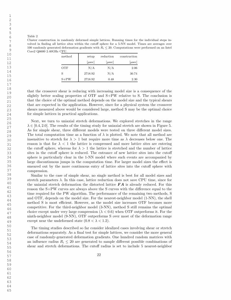
Table 2Cluster construction in randomly deformed simple lattices. Running times for the individual steps in-

volved in finding all lattice sites within the cutoff sphere for a 5-NN model. Times are averages over100 randomly generated deformation gradients with Ri ≤ 20. Computations were performed on an IntelCore2 Q6600 2.40GHz CPU.

method setup reduction construction

[µsec] [µsec] [µsec]

OTF N/A N/A 2.06

S 2718.92 N/A 30.74

S+PW 2718.92 0.48 2.30

that the crossover shear is reducing with increasing model size is a consequence of theslightly better scaling properties of OTF and S+PW relative to S. The conclusion isthat the choice of the optimal method depends on the model size and the typical shearsthat are expected in the application. However, since for a physical system the crossovershears measured above would be considered large, method S may be the optimal choicefor simple lattices in practical applications.

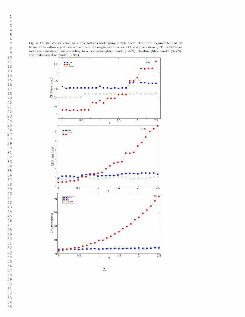
Next, we turn to uniaxial stretch deformations. We explored stretches in the rangeλ ∈ [0.4, 2.0]. The results of the timing study for uniaxial stretch are shown in Figure 5.As for simple shear, three different models were tested on three different model sizes.The total computation time as a function of λ is plotted. We note that all method areinsensitive to stretch for λ > 1 but require more time as λ decreases below one. Thereason is that for λ < 1 the lattice is compressed and more lattice sites are enteringthe cutoff sphere, whereas for λ > 1 the lattice is stretched and the number of latticesites in the cutoff sphere is reduced. The entrance of new lattice sites into the cutoffsphere is particularly clear in the 1-NN model where such events are accompanied bylarge discontinuous jumps in the computation time. For larger model sizes the effect issmeared out by the more continuous entry of lattice sites into the cutoff sphere withcompression.

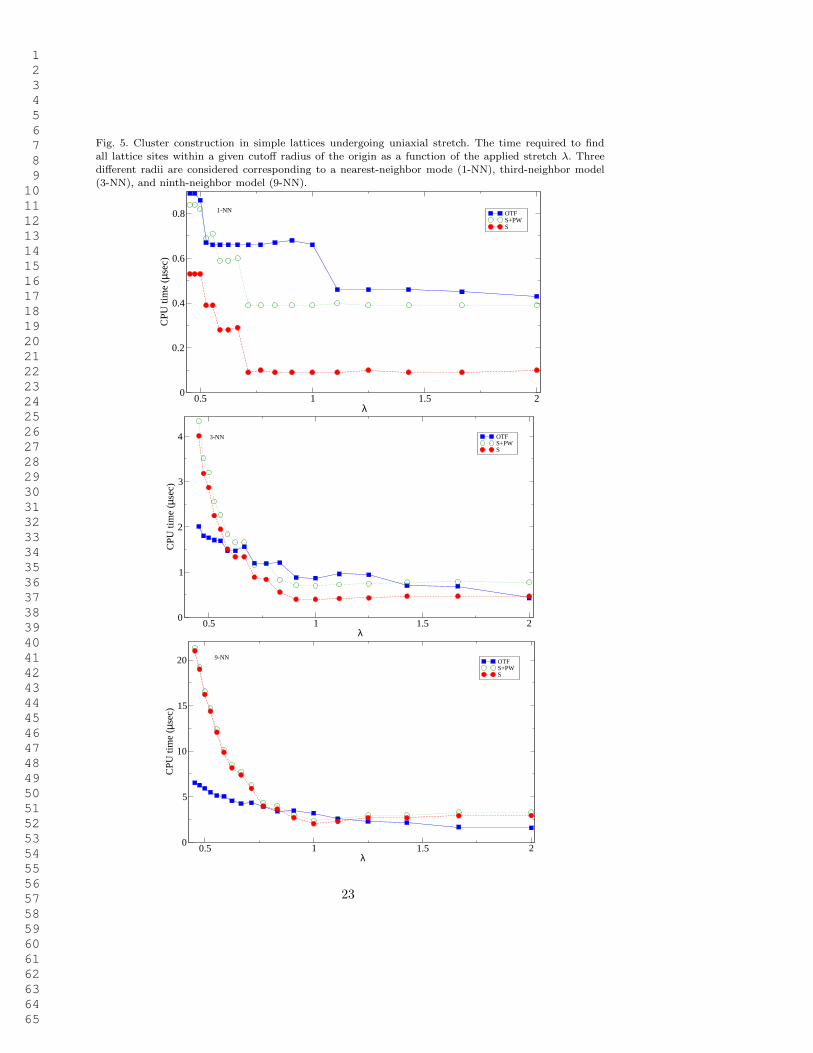
Similar to the case of simple shear, no single method is best for all model sizes andstretch parameters λ. In this case, lattice reduction does not save CPU time, since forthe uniaxial stretch deformation the distorted lattice FA is already reduced. For thisreason the S+PW curves are always above the S curves with the difference equal to thetime required for the PW algorithm. The performance of the remaining two methods, Sand OTF, depends on the model size. For the nearest-neighbor model (1-NN), the shellmethod S is most efficient. However, as the model size increases OTF becomes morecompetitive. For the third-neighbor model (3-NN), method S still remains the optimalchoice except under very large compression (λ < 0.6) when OTF outperforms it. For theninth-neighbor model (9-NN), OTF outperforms S over most of the deformation rangeexcept near the undeformed state (0.8 < λ < 1.2).

The timing studies described so far consider idealized cases involving shear or stretchdeformations separately. As a final test for simple lattices, we consider the more generalcase of randomly-generated deformation gradients. One hundred random matrices withan influence radius Ri ≤ 20 are generated to sample different possible combinations ofshear and stretch deformations. The cutoff radius is set to include 5 nearest-neighbor

22

1 2 3 4 5 6 7 8 9 10 11 12 13 14 15 16 17 18 19 20 21 22 23 24 25 26 27 28 29 30 31 32 33 34 35 36 37 38 39 40 41 42 43 44 45 46 47 48 49 50 51 52 53 54 55 56 57 58 59 60 61 62 63 64 65

Fig. 5. Cluster construction in simple lattices undergoing uniaxial stretch. The time required to findall lattice sites within a given cutoff radius of the origin as a function of the applied stretch λ. Threedifferent radii are considered corresponding to a nearest-neighbor mode (1-NN), third-neighbor model(3-NN), and ninth-neighbor model (9-NN).

0.5 1 1.5 2λ

0

0.2

0.4

0.6

0.8

CPU

tim

e (µ

sec)

OTFS+PWS

1-NN

0.5 1 1.5 2λ

0

1

2

3

4

CPU

tim

e (µ

sec)

OTFS+PWS

3-NN

0.5 1 1.5 2λ

0

5

10

15

20

CPU

tim

e (µ

sec)

OTFS+PWS

9-NN

23

1 2 3 4 5 6 7 8 9 10 11 12 13 14 15 16 17 18 19 20 21 22 23 24 25 26 27 28 29 30 31 32 33 34 35 36 37 38 39 40 41 42 43 44 45 46 47 48 49 50 51 52 53 54 55 56 57 58 59 60 61 62 63 64 65

shells (5-NN). The results are tabulated in Table 2 where the time necessary to setupthe shells and the average times for lattice reduction and for cluster construction areshown. As can be inferred from the Table, the setup stage of the shell methods takes anappreciably large amount of time compared to the time necessary to construct the cluster,while the lattice reduction time is relatively insignificant. Of course, the setup stage onlyneeds to be performed once for a given lattice and is therefore normally inconsequential.Note that the efficiency of OTF and S+PW is comparable with only a slight advantagefor OTF, while method S is not competitive.

4.3. Timing Results for Multilattices

In this section, we discuss the efficiency of methods S, S+PW, and OTF when appliedto multilattices. The nominal lattice is the same cubic lattice used in the previous section.We apply the same shear and stretch deformations to the multilattice as described in thepreceding section for simple lattices and examine the performance of the three methodsfor various model sizes. Our calculations indicate that the methods are insensitive tothe number of sublattices. We therefore only present results for multilattices with twosublattices (2-lattices). To make our timing studies independent of the particular choiceof the sublattice positions, the latter are chosen at random, and the timing results reflectthe average over a set of many multilattices obtained in this manner. We determinedthat a set of 600 randomly distributed samples were sufficient to obtain a convergedaverage. The scatter about the average is displayed in the following graphs as error bars.To accurately measure the CPU time every cluster construction is repeated 104 times.

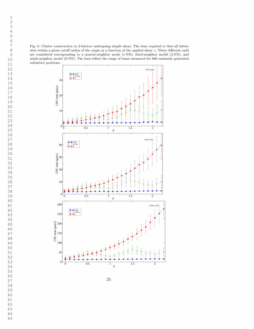
The timing results for the simple shear deformation are displayed in Figure 6. Note thatin contrast to simple lattices, OTF is the most efficient method for any model size andany shear parameter γ. The second best method is S+PW. The additional computationalcost for lattice reduction pays off by considerably decreasing the CPU time relative tomethod S, especially for large values of γ. As before, this is due to lattice invariant shears.The zigzag form of the S+PW curve resulting from this is particularly clear here.

In addition to being the fastest method, OTF also has the advantage that the scatterdue to sublattice positions is minimal. In contrast, both S and S+PW exhibit largescatter. This is due to a noticeable variation in the number of shells that are taken intoaccount for large γ. The number of shells and the influence radius Ri, see (39), dependson the sublattice positions, and therefore varies appreciably when the sublattice positionsare sampled at random.

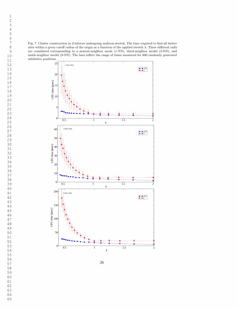
Figure 7 show the results for uniaxial stretch. The timing results S+PW are not dis-played since lattice reduction does not reduce CPU time just as in the case of simplelattices. The conclusions for this deformation are the same as for simple shear. OTF isthe most efficient method for cluster construction for any model size and any stretchparameter λ. The scatter due to sublattice positions remains minimal for OTF, whereasit is significant for method S.

Finally, we consider the general case of randomly-generated deformation gradients. Onehundred random matrices with an influence radius Ri(F , δmax, r) ≤ 20 are generated tosample different possible combinations of shear and stretch deformations. The cutoff

24

1 2 3 4 5 6 7 8 9 10 11 12 13 14 15 16 17 18 19 20 21 22 23 24 25 26 27 28 29 30 31 32 33 34 35 36 37 38 39 40 41 42 43 44 45 46 47 48 49 50 51 52 53 54 55 56 57 58 59 60 61 62 63 64 65

Fig. 6. Cluster construction in 2-lattices undergoing simple shear. The time required to find all latticesites within a given cutoff radius of the origin as a function of the applied shear γ. Three different radiiare considered corresponding to a nearest-neighbor mode (1-NN), third-neighbor model (3-NN), andninth-neighbor model (9-NN). The bars reflect the range of times measured for 600 randomly generatedsublattice positions.

0 0.5 1 1.5 2γ

0

10

20

30

CPU

tim

e (µ

sec)

OTFS+PWS

1-NN-2-BA

0 0.5 1 1.5 2γ

0

20

40

60

80

CPU

tim

e (µ

sec)

OTFS+PWS

3-NN-2-BA

0 0.5 1 1.5 2γ

0

50

100

150

200

250

300

CPU

tim

e (µ

sec)

OTFS+PWS

9-NN-2-BA

25

1 2 3 4 5 6 7 8 9 10 11 12 13 14 15 16 17 18 19 20 21 22 23 24 25 26 27 28 29 30 31 32 33 34 35 36 37 38 39 40 41 42 43 44 45 46 47 48 49 50 51 52 53 54 55 56 57 58 59 60 61 62 63 64 65

Fig. 7. Cluster construction in 2-lattices undergoing uniform stretch. The time required to find all latticesites within a given cutoff radius of the origin as a function of the applied stretch λ. Three different radiiare considered corresponding to a nearest-neighbor mode (1-NN), third-neighbor model (3-NN), andninth-neighbor model (9-NN). The bars reflect the range of times measured for 600 randomly generatedsublattice positions.

0.5 1 1.5 2λ

0

5

10

15

20

25

CPU

tim

e (µ

sec)

OTFS

1-NN-2-BA

0.5 1 1.5 2λ

0

10

20

30

40

50

60

CPU

tim

e (µ

sec)

OTFS

3-NN-2-BA

0.5 1 1.5 2λ

0

50

100

150

200

CPU

tim

e (µ

sec)

OTFS

9-NN-2-BA

26

1 2 3 4 5 6 7 8 9 10 11 12 13 14 15 16 17 18 19 20 21 22 23 24 25 26 27 28 29 30 31 32 33 34 35 36 37 38 39 40 41 42 43 44 45 46 47 48 49 50 51 52 53 54 55 56 57 58 59 60 61 62 63 64 65

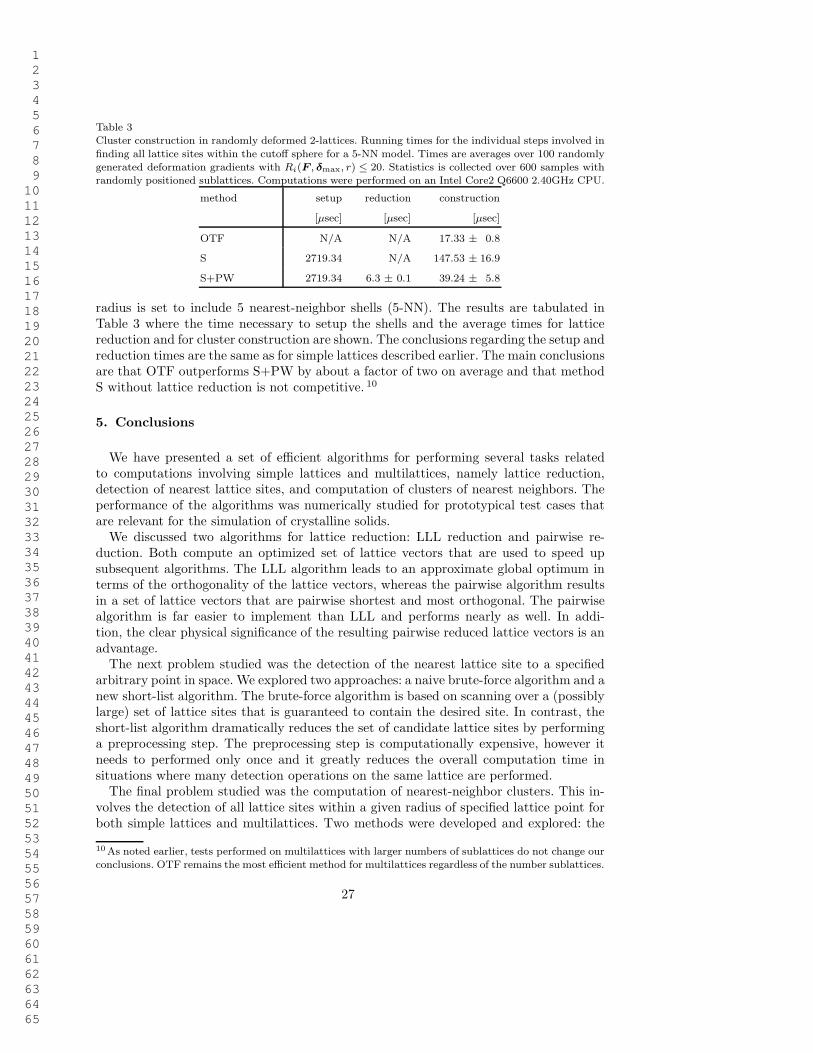
Table 3Cluster construction in randomly deformed 2-lattices. Running times for the individual steps involved in

finding all lattice sites within the cutoff sphere for a 5-NN model. Times are averages over 100 randomlygenerated deformation gradients with Ri(F , δmax, r) ≤ 20. Statistics is collected over 600 samples withrandomly positioned sublattices. Computations were performed on an Intel Core2 Q6600 2.40GHz CPU.

method setup reduction construction

[µsec] [µsec] [µsec]

OTF N/A N/A 17.33 ± 0.8

S 2719.34 N/A 147.53 ± 16.9

S+PW 2719.34 6.3 ± 0.1 39.24 ± 5.8

radius is set to include 5 nearest-neighbor shells (5-NN). The results are tabulated inTable 3 where the time necessary to setup the shells and the average times for latticereduction and for cluster construction are shown. The conclusions regarding the setup andreduction times are the same as for simple lattices described earlier. The main conclusionsare that OTF outperforms S+PW by about a factor of two on average and that methodS without lattice reduction is not competitive. 10

5. Conclusions

We have presented a set of efficient algorithms for performing several tasks relatedto computations involving simple lattices and multilattices, namely lattice reduction,detection of nearest lattice sites, and computation of clusters of nearest neighbors. Theperformance of the algorithms was numerically studied for prototypical test cases thatare relevant for the simulation of crystalline solids.

We discussed two algorithms for lattice reduction: LLL reduction and pairwise re-duction. Both compute an optimized set of lattice vectors that are used to speed upsubsequent algorithms. The LLL algorithm leads to an approximate global optimum interms of the orthogonality of the lattice vectors, whereas the pairwise algorithm resultsin a set of lattice vectors that are pairwise shortest and most orthogonal. The pairwisealgorithm is far easier to implement than LLL and performs nearly as well. In addi-tion, the clear physical significance of the resulting pairwise reduced lattice vectors is anadvantage.

The next problem studied was the detection of the nearest lattice site to a specifiedarbitrary point in space. We explored two approaches: a naive brute-force algorithm and anew short-list algorithm. The brute-force algorithm is based on scanning over a (possiblylarge) set of lattice sites that is guaranteed to contain the desired site. In contrast, theshort-list algorithm dramatically reduces the set of candidate lattice sites by performinga preprocessing step. The preprocessing step is computationally expensive, however itneeds to performed only once and it greatly reduces the overall computation time insituations where many detection operations on the same lattice are performed.

The final problem studied was the computation of nearest-neighbor clusters. This in-volves the detection of all lattice sites within a given radius of specified lattice point forboth simple lattices and multilattices. Two methods were developed and explored: the

10As noted earlier, tests performed on multilattices with larger numbers of sublattices do not change ourconclusions. OTF remains the most efficient method for multilattices regardless of the number sublattices.

27

1 2 3 4 5 6 7 8 9 10 11 12 13 14 15 16 17 18 19 20 21 22 23 24 25 26 27 28 29 30 31 32 33 34 35 36 37 38 39 40 41 42 43 44 45 46 47 48 49 50 51 52 53 54 55 56 57 58 59 60 61 62 63 64 65

shell algorithm and the on-the-fly algorithm. The shell algorithm is based on checkinga set of candidates from a pre-computed sorted crystallite, whereas the on-the-fly algo-rithm provides loops that directly provide the required set of lattice sites at the costof computing complex loop bounds. The performance of the shell method is greatly im-proved if the lattice is reduced in advance. For simple lattices that are not too deformedthe shell method is favorable, whereas for more heavily deformed simple lattices and formultilattices, the on-the-fly method outperforms it by a factor of two on average.

We conclude that the choice of the optimal algorithm for a certain lattice task highlydepends on the setting and the problem data. Even an apparently simple approach, suchas the brute-force algorithm for nearest lattice site detection, can be superior to moreadvanced methods in certain situations. It is therefore essential to estimate the expectedproblem data for the respective application in advance and then to choose the appropriatealgorithm.

The tasks we dealt with in this paper only represent a small subset of tasks that arefrequently encountered during lattice computations. One example is the determinationof the essential unit cell for a multilattice, i.e., given an arbitrary multilattice descrip-tion, to find an optimized description of the multilattice where the number of fractionalposition vectors is smallest and their lengths are shortest. Another common task is givena triangulation where the nodes are lattice sites, to find the cell that contains an ar-bitrary specified lattice site. An efficient algorithm would exploit the underlying latticestructure to speed up the search compared to classical approaches like oct-tree methodsfor triangulations with arbitrary nodes. However, these tasks and others are beyond thescope of this paper.

Appendix

Several proofs have been omitted in the text in order not to interrupt the flow by toomany technical details. We make up for this now.

A.1. Pairwise Lattice Reduction

First we start with two properties from Section 2 regarding length reduction and anglereduction.

Lemma A.1 Let ai, aj ∈ Rd be two linearly independent vectors. If ai is length-reduced

by aj, that is

‖ai − maj‖ ≥ ‖ai‖ (A.1)

for all m ∈ Z, then ai is angle-reduced to aj as well, i.e., ai is the vector among all

ai − maj whose angle with aj is closest to 90 or π2 in radians,

∣

∣

∣∠(ai − maj , aj) −

π

2

∣

∣

∣≥

∣

∣

∣∠(ai, aj) −

π

2

∣

∣

∣(A.2)

for all m ∈ Z.

Proof Because

cos∠(ai − maj , aj) =|(ai − maj) · aj |‖ai − maj‖‖aj‖

, (A.3)

28

1 2 3 4 5 6 7 8 9 10 11 12 13 14 15 16 17 18 19 20 21 22 23 24 25 26 27 28 29 30 31 32 33 34 35 36 37 38 39 40 41 42 43 44 45 46 47 48 49 50 51 52 53 54 55 56 57 58 59 60 61 62 63 64 65

we need to show that (A.1) is equivalent to

|(ai − maj) · aj |‖ai − maj‖‖aj‖

≥ |ai · aj |‖ai‖‖aj‖

(A.4)

for all m ∈ Z. Squaring and multiplying out the terms gives that (A.4) is equivalent to(

(ai · aj)2 − 2m(ai · aj)‖aj‖2 + m2‖aj‖4

)

‖ai‖2

≥ (ai · aj)2(

‖ai‖2 − 2m(ai · aj) + m2‖aj‖2)

.(A.5)

Rearranging terms leads to(

−2m(ai · aj) + m2‖aj‖2) (

‖ai‖2‖aj‖2 − (ai · aj)2)

≥ 0. (A.6)

The second factor on the left side of the inequality is always positive because ai and aj

are linearly independent. Therefore (A.6) is equivalent to

−2m(ai · aj) + m2‖aj‖2 ≥ 0. (A.7)

Adding ‖ai‖2 to both sides shows that (A.7) is equivalent to (A.1). 2

Lemma A.2 If some longer vector al ∈ Rd is length-reduced by some shorter vector

as ∈ Rd, i.e., ‖al‖ ≥ ‖as‖ and ‖al −mas‖ ≥ ‖al‖ for all m ∈ Z, then the shorter vector

as is automatically length-reduced by the longer vector al as well, i.e., ‖as−mal‖ ≥ ‖as‖for all m ∈ Z.

Proof We have that

‖as − mal‖2 − ‖as‖2 = −2m(as · al) + m2‖al‖2

≥ −2m(as · al) + m2‖as‖2

= ‖al − mas‖2 − ‖al‖2

≥ 0.

(A.8)

2

A.2. Search Range for Short-List Method

Next, we come to the derivation of the search range, Rsl, for the short-list methoddescribed in Section 3.2. Recall that Rsl consists of (at least) all lattice sites that are

closest to at least one point in A[

− 12 , 1

2

]d. The search range, Rsl, needs to be determined

in a preprocessing step.The key to this preprocessing step are Voronoi cells, also referred to as Wigner-Seitz

cells in physics. The Voronoi cell V(n) of some lattice point An is defined as

V(n) :=

x ∈ Rd : ‖An − x‖ ≤ ‖Am − x‖ ∀m ∈ Z

d

, (A.9)

i.e., the set of all points x to which An is the closest lattice point. It can be shown thatV(n) is the intersection

V(n) =⋂

m∈Zd,m 6=n

H(n, m) (A.10)

of half-spaces H(n, m) defined by (24). Note that the half-space H(n, m) contains An

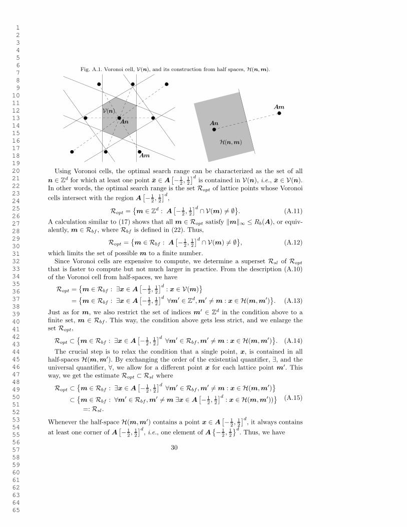
and is bounded by the plane that is perpendicular to the line from An to Am and thatgoes through the midpoint of An and Am. The construction of the Voronoi cell fromhalf-spaces is illustrated in Figure A.1.

29

1 2 3 4 5 6 7 8 9 10 11 12 13 14 15 16 17 18 19 20 21 22 23 24 25 26 27 28 29 30 31 32 33 34 35 36 37 38 39 40 41 42 43 44 45 46 47 48 49 50 51 52 53 54 55 56 57 58 59 60 61 62 63 64 65

Fig. A.1. Voronoi cell, V(n), and its construction from half spaces, H(n, m).

V(n)

An

Am

An

Am

H(n,m)

Using Voronoi cells, the optimal search range can be characterized as the set of all

n ∈ Zd for which at least one point x ∈ A

[

− 12 , 1

2

]dis contained in V(n), i.e., x ∈ V(n).

In other words, the optimal search range is the set Ropt of lattice points whose Voronoi

cells intersect with the region A[

− 12 , 1

2

]d,

Ropt =

m ∈ Zd : A

[

− 12 , 1

2

]d ∩ V(m) 6= ∅

. (A.11)

A calculation similar to (17) shows that all m ∈ Ropt satisfy ‖m‖∞ ≤ Rb(A), or equiv-alently, m ∈ Rbf , where Rbf is defined in (22). Thus,

Ropt =

m ∈ Rbf : A[

− 12 , 1

2

]d ∩ V(m) 6= ∅

, (A.12)

which limits the set of possible m to a finite number.Since Voronoi cells are expensive to compute, we determine a superset Rsl of Ropt

that is faster to compute but not much larger in practice. From the description (A.10)of the Voronoi cell from half-spaces, we have

Ropt =

m ∈ Rbf : ∃x ∈ A[

− 12 , 1

2

]d: x ∈ V(m)

=

m ∈ Rbf : ∃x ∈ A[

− 12 , 1

2

]d ∀m′ ∈ Zd, m′ 6= m : x ∈ H(m, m′)

. (A.13)

Just as for m, we also restrict the set of indices m′ ∈ Zd in the condition above to a

finite set, m ∈ Rbf . This way, the condition above gets less strict, and we enlarge theset Ropt,

Ropt ⊂

m ∈ Rbf : ∃x ∈ A[

− 12 , 1

2

]d ∀m′ ∈ Rbf , m′ 6= m : x ∈ H(m, m′)

. (A.14)

The crucial step is to relax the condition that a single point, x, is contained in allhalf-spaces H(m, m′). By exchanging the order of the existential quantifier, ∃, and theuniversal quantifier, ∀, we allow for a different point x for each lattice point m′. Thisway, we get the estimate Ropt ⊂ Rsl where

Ropt ⊂

m ∈ Rbf : ∃x ∈ A[

− 12 , 1

2

]d ∀m′ ∈ Rbf , m′ 6= m : x ∈ H(m, m′)

⊂

m ∈ Rbf : ∀m′ ∈ Rbf , m′ 6= m ∃x ∈ A[

− 12 , 1

2

]d: x ∈ H(m, m′))

=: Rsl.

(A.15)

Whenever the half-space H(m, m′) contains a point x ∈ A[

− 12 , 1

2

]d, it always contains

at least one corner of A[

− 12 , 1

2

]d, i.e., one element of A

− 12 , 1

2

d. Thus, we have

30

1 2 3 4 5 6 7 8 9 10 11 12 13 14 15 16 17 18 19 20 21 22 23 24 25 26 27 28 29 30 31 32 33 34 35 36 37 38 39 40 41 42 43 44 45 46 47 48 49 50 51 52 53 54 55 56 57 58 59 60 61 62 63 64 65

Rsl =

m ∈ Rbf : ∀m′ ∈ Rbf , m′ 6= m ∃x ∈ A

− 12 , 1

2

d: x ∈ H(m, m′)

=

m ∈ Rbf : ∀m′ ∈ Rbf , m′ 6= m : A

− 12 , 1

2

d ∩H(m, m′) 6= ∅

,(A.16)

which is precisely the definition (23) of Rsl in Section 3.2. Note that (A.16) is based ona finite number of possible vectors m, m′ and corner points x that need to be checkedagainst each other by the half-space condition, x ∈ H(m, m′). This makes the searchrange actually computable. See Algorithm 3.

A.3. On-the-Fly Method for Cluster Computation

Finally, we come to a property used in the on-the-fly algorithm for cluster computationin Section 4.1.2.

Lemma A.3 Let

G =

G g

gT γ

∈ Rd×d (A.17)

with G ∈ R(d−1)×(d−1), g ∈ R

d−1, γ ∈ R be a symmetric positive definite matrix. Then

G := G − g ⊗ g

γ∈ R

(d−1)×(d−1) (A.18)

is symmetric positive definite as well.

Proof G is symmetric by definition. We need to show that xT Gx > 0 for any givennon-zero vector x ∈ R

d−1. Define

x :=

x

ξ

∈ Rd with ξ := −gT x

γ∈ R. (A.19)

Then x 6= 0, and xT Gx > 0 because G is positive definite. We thus have

xT Gx = xT Gx − (gT x)2

γ

= xT Gx + 2ξgT x + γξ2

= xT Gx

> 0,

(A.20)

thus G is positive definite. 2

Acknowledgements

This work was supported in part by the Department of Energy under Award NumberDE-FG02-05ER25706 and by the University of Minnesota Supercomputing Institute. Theauthors acknowledge preliminary work performed by Jon Wilkening on the “short-list”method, while working as a postdoctoral fellow on quasicontinuum applications. Theauthors would like to thank Ryan Elliott for his careful reading of the manuscript andmany helpful comments.

31

1 2 3 4 5 6 7 8 9 10 11 12 13 14 15 16 17 18 19 20 21 22 23 24 25 26 27 28 29 30 31 32 33 34 35 36 37 38 39 40 41 42 43 44 45 46 47 48 49 50 51 52 53 54 55 56 57 58 59 60 61 62 63 64 65

References

[1] E. Agrell, T. Eriksson, A. Vardy, K. Zeger, Closest point search in lattices, IEEETrans. Inf. Theory 48 (8) (2002) 2201–2214.

[2] J. W. S. Cassels, An introduction to the geometry of numbers, vol. 99 ofGrundlehren der mathematischen Wissenschaften in Einzeldarstellungen mit beson-derer Berucksichtigung der Anwendungsgebiete, Springer-Verlag, Berlin, Heidelberg,New York, 1971.

[3] M. Dobson, R. S. Elliott, M. Luskin, E. B. Tadmor, A multilattice quasicontinuumfor phase transforming materials: Cascading Cauchy Born kinematics, J. Comput.-Aided Mater. Des. 14 (Supplement 1) (2007) 219–237.

[4] C. F. Gauss, Disquisitiones Arithmeticae, Yale University Press, New Haven, Lon-don, 1801, transl. A. A. Clarke, 1966.

[5] R. Kannan, Algorithmic geometry of numbers, Annu. Rev. Comput. Sci. 2 (1987)231–267.

[6] K. Kremer, K. Binder, Monte carlo simulations of lattice models for macromolecules,Comp. Phys. Reports 7 (1988) 259–310.

[7] A. K. Lenstra, H. W. Lenstra Jr., L. Lovasz, Factoring polynomials with rationalcoefficients, Math. Ann. 261 (1982) 515–534.

[8] B. M. McCoy, T. T. Wu, The Two-Dimensional Ising Model, Harvard UniversityPress, Cambridge, 1973.

[9] G. P. Parry, On essential and non-essential descriptions of multilattices, Math. Mech.Solids 9 (2004) 411–418.

[10] M. Pitteri, Geometry and symmetry of multilattices, Int. J. Plast. 14 (1998) 139–157.[11] W. H. Press, S. A. Teukolsky, W. T. Vetterling, B. P. Flannery, Numerical Recipes

in FORTRAN. The art of scientific computing, 2nd ed., Cambridge University Press,Cambridge, 1992.

[12] V. B. Shenoy, R. Miller, E. B. Tadmor, D. Rodney, R. Phillips, M. Ortiz, An adaptivefinite element approach to atomic-scale mechanics — the quasicontinuum method,J. Mech. Phys. Solids 47 (3) (1999) 611–642.

[13] E. B. Tadmor, M. Ortiz, R. Phillips, Quasicontinuum analysis of defects in solids,Philos. Mag. A 73 (6) (1996) 1529–1563.

[14] E. B. Tadmor, G. S. Smith, N. Bernstein, E. Kaxiras, Mixed finite element andatomistic formulation for complex crystals, Phys. Rev. B 59 (1) (1999) 235–245.

[15] K. Yue, K. M. Fiebig, P. D. Thomas, H. S. Chan, E. I. Shakhnovich, K. A. Dill,A test of lattice protein folding algorithms, Proc. Natl. Acad. Sci. USA 92 (1995)325–329.

32