ediss.sub.uni-hamburg.de · introduction numerical simulation of physical, biological, chemical and...

A General Approach to theDiscretization of

Hyperbolic Conservation Lawson Unstructured Grids

Dissertation

zur Erlangung des Doktorgrades

des Fachbereichs Mathematik

der Universitat Hamburg

vorgelegt von

Arne Ahrend

aus Hildesheim

Hamburg

1999

Als Dissertation angenommen vom FachbereichMathematik der Universitat Hamburg

auf Grund der Gutachten von Prof. Dr. Thomas Sonarund Prof. Dr. Rainer Ansorge

Hamburg, den 20. August 1999

Prof. Dr. Hans DadunaDekan des Fachbereichs Mathematik

Contents

Introduction 4

1 Conservation Laws 71.1 Fundamental Principles . . . . . . . . . . . . . . . . . . . . . . 71.2 Scalar Equations . . . . . . . . . . . . . . . . . . . . . . . . . 10

Linear Advection . . . . . . . . . . . . . . . . . . . . . . . . . 10Characteristics . . . . . . . . . . . . . . . . . . . . . . . . . . 14Discontinuities and Self Similarity . . . . . . . . . . . . . . . . 15Weak Solutions . . . . . . . . . . . . . . . . . . . . . . . . . . 17Diffusion and Entropy . . . . . . . . . . . . . . . . . . . . . . 18Upwinding and the Equal Area Rule . . . . . . . . . . . . . . 20Construction Criteria for Weak Solutions . . . . . . . . . . . . 22Numerical Flux Functions . . . . . . . . . . . . . . . . . . . . 24Burgers Equation . . . . . . . . . . . . . . . . . . . . . . . . . 27

1.3 Hyperbolic Systems . . . . . . . . . . . . . . . . . . . . . . . . 28The Covariant Formulation . . . . . . . . . . . . . . . . . . . . 28Symmetry and Hyperbolicity . . . . . . . . . . . . . . . . . . . 28The Riemann Problem and Riemann Invariants . . . . . . . . 31Numerical Flux Functions . . . . . . . . . . . . . . . . . . . . 38

2 Discretization 432.1 Data Functionals . . . . . . . . . . . . . . . . . . . . . . . . . 432.2 Unstructured Grids . . . . . . . . . . . . . . . . . . . . . . . . 47

Construction of Boxes . . . . . . . . . . . . . . . . . . . . . . 49Collocation Grids . . . . . . . . . . . . . . . . . . . . . . . . . 49

2.3 Boundary Conditions . . . . . . . . . . . . . . . . . . . . . . . 512.4 Time Integration . . . . . . . . . . . . . . . . . . . . . . . . . 522.5 The Finite Volume Method . . . . . . . . . . . . . . . . . . . 532.6 Reconstruction . . . . . . . . . . . . . . . . . . . . . . . . . . 56

Approximation . . . . . . . . . . . . . . . . . . . . . . . . . . 58Stencil Selection . . . . . . . . . . . . . . . . . . . . . . . . . . 65

3

4 INTRODUCTION

Oscillation Indicators . . . . . . . . . . . . . . . . . . . . . . . 672.7 Numerical Divergence Operator . . . . . . . . . . . . . . . . . 68

Approximation of Linear Functionals . . . . . . . . . . . . . . 69The Divergence Functional . . . . . . . . . . . . . . . . . . . . 74

2.8 The CFL Condition . . . . . . . . . . . . . . . . . . . . . . . . 76

3 The Euler Equations of Gas Dynamics 793.1 The Euler Flux Function . . . . . . . . . . . . . . . . . . . . . 793.2 Riemann Invariants . . . . . . . . . . . . . . . . . . . . . . . . 823.3 Jump Relations . . . . . . . . . . . . . . . . . . . . . . . . . . 843.4 Numerical Flux Functions . . . . . . . . . . . . . . . . . . . . 853.5 Boundary Conditions . . . . . . . . . . . . . . . . . . . . . . . 88

4 Collocation Schemes 894.1 The Lax-Friedrichs Scheme . . . . . . . . . . . . . . . . . . . . 89

Cartesian Grids . . . . . . . . . . . . . . . . . . . . . . . . . . 89Unstructured Grids . . . . . . . . . . . . . . . . . . . . . . . . 92

4.2 Upwinding Schemes . . . . . . . . . . . . . . . . . . . . . . . . 94Choice of Data Locations . . . . . . . . . . . . . . . . . . . . . 95

4.3 Numerical Experiments . . . . . . . . . . . . . . . . . . . . . . 962D Shock Tube for the Euler Equations . . . . . . . . . . . . . 96Double Mach Reflection . . . . . . . . . . . . . . . . . . . . . 98

A Measure of d-dimensional simplex 101

B List of Symbols 103

Bibliography 107

Danksagung 113

Abstract 115

Zusammenfassung 117

Lebenslauf 119

Introduction

Numerical simulation of physical, biological, chemical and even financial pro-cesses is becoming an increasingly widespread technique and replacing moretime and money consuming experimental techniques like the building of mod-els. Next to savings in expenditure this is due to the great flexibility of usinga computer that allows rapid adaption of the investigated configuration.

Many natural and technical processes are governed by simple principles,like minimization of convex functionals or conservation of certain quantities.This thesis is devoted to the study of numerical methods to simulate thelatter ones. In particular we develop a collocation method for hyperbolicconservation laws which is capable of adequately resolving strong shocks intransonic flow fields. The robustness and accuracy of the method is demon-strated by certain well established test cases for the Euler equations of gasdynamics.

Given the great success of finite volume methods (besides their formalelegance) considering collocation methods today perhaps requires some jus-tification. The finite volume method combines a discrete integral formulationof the conservation principle with a rich geometric data structure. The stateof the art in two dimensions is marked by adaptive methods using eithercartesian grids or conforming simplex grids with boxes. Simplex grids inparticular allow flexible and automatic discretization of complex geometriesand we focus our considerations on equally unstructured and flexible grids.

One urgent demand arising from practical applications is the extension ofcontemporary methods from two to three space dimensions. Unfortunately,the generation of regular simplex grids in higher dimensions is a hard prob-lem. For this reason one might look for ways to weaken the geometricalstructure that underpins the finite volume method. A collocation schemethat operates on sets of smoothly scattered points and only requires someinformation about neighbourhood relations between these points would beeasier to implement in higher dimensions than methods that work on tes-salations.

In the course of developing such a method one is presented with formidable

5

6 INTRODUCTION

technical difficulties. One important property of a program for simulatingtransonic gas flow, for example, is the capability of handling discontinuities.Finite volume methods achieve this via the solution of locally one dimen-sional Riemann problems. We have been able to design a similar mechanismfor the collocation case by considering edges between neighbouring pointsand fluxes essentially directed along these edges.

Another motive for considering collocation functionals is the desire touse arbitrary trial spaces for which cell averaging functionals might be tooexpensive to handle. The polynomial recovery techniques widely used todaywork quite well, but they are largely based on heuristics. In particular,there is no rigorous theory of oscillation indicators and reconstruction weightsavailable. Only very recently have mathematicians begun to look into theseproblems systematically. Collecting practical experience with generalizationsof the methods that are so well-established today can perhaps help to pavea road towards a scheme that is both computationally efficient and foundedon a comprehensive theory.

In chapter one of this thesis we discuss the features of hyperbolic conser-vation laws in some depth focusing on the topics relevant to schemes withupwind properties. We analyze the flux across discontinuities and classifynumerical flux functions by the way they differ from the plain average of thefluxes to the left and right of the discontinuity.

The second chapter is concerned with discretization techniques. It intro-duces the grids we consider and presents a general framework of discretizationwhich comprises both finite volume and collocation methods. We demon-strate uniform stability of the reconstruction process under similarity trans-formations of the grid for both collocation and cell averaging functionals.

In the third chapter we review the Euler equations of gas dynamics, per-haps the most important and well-studied hyperbolic system. It is closelyrelated to the discussion in the first chapter, however, placing it here stressesthat the discretization techniques developed in the second chapter are notspecific to the Euler equations.

The fourth chapter finally contains a few remarks on our early attemptsand numerical examples for some commonly accepted test cases for Eulercomputations generated with the current version of our collocation method.

Chapter 1

Conservation Laws

1.1 Fundamental Principles

If a quantity M is conserved within a region Ω, any change of the amount ofM contained in Ω corresponds to transport of M across the boundary of Ω.

Under the assumption that there is a finite upper bound on the velocitywith which either the quantity M or the region Ω may move along, theconservation principle has a far reaching immediate consequence:

During a short interval in time all changes of the amount of Mcontained in Ω depend only on the distribution of M in a layerabout the boundary of Ω. It does not matter how M is distributeddeep inside Ω or far away from it.

In order to express the above principle in the language of mathematics, weintroduce the following abstractions and definitions:

Definition 1.1. A control volume or cell is a fixed (not moving) compactpolyhedron1 Σ ⊂ Rd

Polyhedra allow H1 approximation of smooth geometries, and in order toimprove the geometric approximation, it may sometimes be desirable to relaxthe above definition in the following way: given a “reasonably good” Hk

approximation of a sufficiently smooth geometrical object, the surfaces ofthe control volumes may be modified to yield an Hk+1 approximation of theobject under consideration.

More general notions of a control volume may be envisaged, like that ofa connected bounded set whose boundary has a piecewise continuous outer

1a non empty connected set with intΣ = Σ whose boundary is formed by a finitenumber of subsets of hyperplanes

7

8 CHAPTER 1. CONSERVATION LAWS

normal ~n. The key point in any such definition is the availability of somevariant of the divergence theorem, but there would be no substantial benefitin using those generalizations here.

Let M take values in Rs and M(t, Σ) denote the amount of M in the

control volume Σ at time t. Finally assume that the movement of M at timet and point ~x is described by a flux j(t, ~x) ∈ Rs×d. Now the conservationprinciple can be stated in integral formulation:

M(t, Σ) = M(t0, Σ) −∫ t

t0

∫∂Σ

j~n do.

Transport out of Σ decreases the components of M(t, Σ), but for such trans-port the integrand on the right hand side is positive, as ~n is the outer normal.

Definition 1.2. A function u : R × Rd → S is called density of M at the

point ~x ∈ Rd at time t, if for any control volume Σ ⊂ Rd

M(t, Σ) =

∫Σ

u(t, ~x) dV.

S ⊂ Rs is called state space and Rd physical space or just space.

Throughout this thesis we will only consider quantities which have densitiesand speak of the conservation of the abstract quantities and their densitiessynonymously.

The conservation principle may now be restated in terms of the density:∫Σ

u(t, ~x) dV =

∫Σ

u(t0, ~x) dV −∫ t

t0

∫∂Σ

j~n do (1.1a)

or after differentiation with respect to time

d

dt

∫Σ

u(t, ~x) dV = −∫

∂Σ

j~n do. (1.1b)

If the functions in equations (1.1) are sufficiently smooth, we may swapdifferentiation with respect to time and spatial integration on the left handside and use the divergence theorem on the right hand side to obtain2∫

Σ

∂

∂tu(t, ~x) dV = −

∫Σ

divj dV.

2All vector operations are carried out on each state component separately.

1.1. FUNDAMENTAL PRINCIPLES 9

For the class of Σ’s we are considering this implies that the integrands mustmatch pointwise, hence

∂

∂tu + div j = 0. (1.2)

Equation (1.2) is called the differential form of the conservation principle.For physical phenomena the flux should not explicitly depend on the timeand space coordinates, since the forms of the laws of nature should not hingeon any particular frame of reference imposed by an observer [Ein05]. If theflux thus depends on u alone and is C1, then j = F u with a (smoothcase) flux function F := (F 1, . . . , F d) : S → Rs×d with F k : Rs → Rs, andequation (1.2) can be stated in quasi-linear form:

∂

∂tu +

d∑k=1

∂F k

∂u

∂u

∂xk= 0. (1.3)

We will assume throughout this thesis that F ∈ C2(S → Rs×d).The problems we will study in this thesis consist of a conservation law in

either of the above forms, a prescribed domain Ω, an initial density distribu-tion u0(~x) = u(t0, ~x) on Ω and boundary conditions on the fluxes across theboundary of Ω: for ~x ∈ ∂Ω

F (u(t, ~x))~n = B(u, t, ~x). (1.4)

Restricting F to be dependent on u alone precludes modeling inhomogenitiesin space, source terms, certain kinds of boundary conditions and diffusive ef-fects. In many applications, however, the flux function is simply a sum of aconvective term (depending on u alone), a diffusive term that depends essen-tially on ∇u alone and source terms which mainly depend on space and timecoordinates. Furthermore, these additional terms satisfy certain regularityconditions, cf. [Maj84] for a detailed discussion, and may consequently beregarded as small corrections to the convective term. A flux with a diffusivecomponent has the form

F (u) − A∇u

where A = A(u, t, ~x) is always a diagonalizable positive semi-definite ma-trix. Roughly speaking the term −A∇ contributes downhill transport, lo-cally levelling u. If A had negative eigenvalues, then there would occur uphilltransport, causing small differences to blow up, similar to the behaviour of a“backward heat transport equation”. The solution to such a problem expo-nentially blows up in time, and a numerical scheme simulating it cannot bestable.


Modeling just the convective flux entails a number of interesting diffi-culties – the spontaneous generation of discontinuities is perhaps the mostnotable of these – that translate into certain strategies for implementingnumerical schemes for conservation laws. In this thesis we shall almost ex-clusively contemplate convective phenomena.

1.2 Scalar Equations

Linear Advection

Consider an initial scalar density distribution u0 : Rd → R at time t0 beingshifted by multiples of a constant vector ~ν ∈ R

d:

u(t, ~x) := u0(~x − ~ν(t − t0)). (1.5)

Obviously u is conserved. Furthermore, if u0 is a smooth function, u(t, ·)will always be smooth, as it is simply a shifted version of u0. We may thusdifferentiate with respect to time and space:

∂

∂t

∣∣∣∣t,~x

u = −~ν · ∇|~x−~ν(t−t0)u0

∇|t,~xu = ∇|~x−~ν(t−t0)u0

Taking into account that div ~νu0 = ~ν ·∇u0 we infer that the differential form(1.2) of the conservation law is satisfied, if and only if we define the flux by

j := F (u) := u~ν t.

We now apply the integral formulation of equations (1.1) of the conservationprinciple to a certain class of discontinuous functions u0 in order to derivea definition of the flux which will satisfy (1.5) at discontinuities. Whilethere is no hope of managing a completely random function u0, the conserva-tion principle may be successfully applied to an initial distribution u0 whosediscontinuities are aligned with the interfaces of suitably chosen control vol-umes. It turns out that the flux across such a discontinuity is a function ofthe states at both sides of the discontinuity and the direction normal to it.This function is called the Riemann solver for the flux F . Later we willdevelop approximate Riemann solvers for non-linear systems of hyperbolicconservation laws.

1.2. SCALAR EQUATIONS 11

Proposition 1.3. Let Σ be a cell. Assume that u0 : Rd → R is a boundedpiecewise continuous function which is continuous inside Σ and can be con-tinuously extended to Σ from the inside and piecewise continuously to R

d \(int Σ) from the outside. On the boundary of Σ define almost everywhere

ui(~x) := lim~y→~x

u0(~y) (~y ∈ int Σ)

uo(~x) := lim~y→~x

u0(~y) (~y 6∈ Σ).(1.6)

Then the integral formulation (1.1) of the conservation principle is satisfied,if and only if we define the Riemann solver

F (ui, uo, ~n) := j~n :=

~ν · ~nui if ~ν · ~n > 0

~ν · ~nuo if ~ν · ~n < 0(1.7)

almost everywhere on ∂Σ.

Before presenting the proof we observe that the definition of ui and uo in(1.6) depends on the particular Σ under consideration, but the Riemannsolver F (ui, uo, ~n) in (1.7) does not. On a common interface between anytwo control volumes Σ and Σ′ with outer normals ~n and ~n′ respectively onehas almost everywhere: ~n = −~n′, ui = u′

o, uo = u′i – the inner limit as seen

from Σ is the outer limit as seen from Σ′ and vice versa – and consequentlyF (ui, uo, ~n) = j~n = −j~n′ = −F (u′

i, u′o, ~n

′).

Proof of proposition 1.3. We first establish by indirect proof that the defini-tion in equation (1.7) is necessary. Let us assume that the Riemann solvercould be defined otherwise.

There are then a unit vector ~q ∈ Rd and two numbers ul, ur ∈ R for which

a flux different from that of equation (1.7) will satisfy the integral form ofthe conservation law. Now let

u0(~x) :=

ul if ~x · ~q 6 0

ur if ~x · ~q > 0.

Since the density distribution is known, we may compute the content of anoblique cylinder or prism Θ of height h and cross section – parallel to thehyperplane – A (Volume V = Ah) with one end initially on the hyperplane~x · ~q = 0 and outer normal ~q for this end (i.e. Θ lies initially to the left of thehyperplane, see figure 1.1). For t ∈ [t0, t0 + h/ |~ν · ~q|) one has

M(t, Θ) =

ulAh if ~ν · ~q > 0

[(ul − ur)(t − t0) ~ν · ~q + ulh]A if ~ν · ~q < 0


h

q

A

Figure 1.1: The cylinder Θ and the unit vector ~q on the hyperplaneseparating the states ul and ur. If ~ν · ~q < 0, the hyperplane movesleft and ur “enters” Θ, otherwise Θ will always contain only ul.

which implies

d

dt

∣∣∣∣t0+

M(t, Θ) =

0 if ~ν · ~q > 0

(ul − ur) ~ν · ~q A if ~ν · ~q < 0.

On the other hand all fluxes across the jacket cancel out∫∂Θ

j~n do = (F (ul, ur, ~q) − F (ul)~q)A

and by virtue of the conservation principle in equations (1.1) we obtain acontradiction to our assumption:

F (ul, ur, ~q), q) = F (ul)~q − 1

A

d

dt

∣∣∣∣t0+

M(t, Θ) =

~ν · ~q ul if ~ν · ~q > 0

~ν · ~q ur if ~ν · ~q < 0.

The proof of sufficiency is straightforward, but technical. By assumption u0

can be continuously extended to Σ which is compact. Hence u0 is uniformlycontinuous on any subset of Σ. Similarly, for a compact set Ξ with Σ ⊂ int Ξ,u0 is uniformly continuous on the intersection of any continuity componentadjacent to Σ with Ξ \Σ. Subdivide Σ into a finite number of closed convexpolyhedra Σ1, . . . , ΣN and each Σk into subsets Θ such that

• each Θ is the intersection of Σk and a prism or cylinder with axisparallel to ~ν and

• any intersections of edges of Σk with Θ are aligned with edges of Θ.


Θ is convex and the flux across its jacket – the part of its boundary formedby the jacket of a cylinder – is pointwise zero, because ~ν · ~n = 0 for anynormal ~n on the jacket.

Denote by Θ1 the surface part of Θ for which ~ν · ~n < 0, and by Θ2

the opposite end. Now by a reasoning similar to that above and the Fubinitheorem on integration on product spaces

M(t, Θ) = M(t0, Θ) +

∫Θ1

∫ t

t0

u(τ, ~x) dτ do −∫

Θ2

∫ t

t0

u(τ, ~x) dτ do

= M(t0, Θ) +

∫Θ1

∫ t

t0

u0(~x − τ~ν) dτ do −∫

Θ2

∫ t

t0

u0(~x − τ~ν) dτ do

and uniform continuity permits swapping integration over Θ1,2 and the limesof the difference quotient

d

dt

∣∣∣∣t0+

M(t, Θ) =

∫Θ1

‖~ν‖ limτt0

u0(~x − τ~ν) do −∫

Θ2

‖~ν‖ limτt0

u0(~x − τ~ν) do

=

∫Θ1

‖~ν‖ limτ0

u(t0, ~x − τ~ν) do −∫

Θ2

‖~ν‖ limτ0

u(t0, ~x − τ~ν) do

= −∫

∂Θ

F (ui, uo, ~n) do.

Summation over all Θ completes the proof.

We conclude this paragraph by summarizing (without proof) some algebraicproperties of the Riemann solver:

Lemma 1.4. Let ~n ∈ Rd be an arbitrary unit vector. The Riemann solverof equation (1.7)

1. is consistent with the flux function in the following way:∣∣∣∣F (ui, uo, ~n) − F (ui) + F (uo)

2~n

∣∣∣∣ ≤ ‖~ν‖Rd

|ui − uo|2

,

2. may equivalently be written as

F (ui, uo, ~n) =F (ui) + F (uo)

2~n + |~ν · ~n| ui − uo

2

3. and obeys

F (ui, uo, ~n) = −F (uo, ui,−~n).


Characteristics

Direction and velocity of the density profiles propagation in the linear ad-vection equation above were those of the vector ~ν ∈ Rd in

∂

∂tu + ~ν · ∇u = 0.

Let us now consider the case of a scalar conservation law with a non lineardifferentiable flux j = F (u) ∈ R1×d depending on u alone. Let C ⊂ R be aninterval of length greater than zero.

Definition 1.5. A continuous function χ : C → Rd is called a characteristiccurve for the quasi-linear equation (1.3), if for t0 ∈ C fixed and any t ∈ C:

u(t, χ(t)) = u(t0, χ(t0)). (1.8)

In the scalar case the characteristics are essentially straight lines in the di-rection of F ′(u). This implies that F ′ u plays the role of a characteristicvelocity field: in smooth regions of u small local phenomena travel at velocityF ′(u).

Lemma 1.6. With the same expressions as in the preceding definition as-sume that χ : C → Rd is differentiable and u is smooth on an open setcontaining

(t, χ(t)) ∈ C × R

d : t ∈ C. Then the lines defined by

χt(t) := χt(t0) + (t − t0)F′(u(t0, χ(t0))) (1.9)

are characteristics.

Proof. Differentiate (1.8) with respect to time:

0 =d

dτ

∣∣∣∣t

u(τ, χ(τ)) by (1.8)

=∂

∂τ

∣∣∣∣t

u +

(d

dτ

∣∣∣∣t

χt

)∇|(t,χ(t))u by the chain rule

=

(d

dτ

∣∣∣∣t

χt − F ′∣∣∣∣u(t,χ(t))

)∇|(t,χ(t))u by (1.3)

=

(d

dτ

∣∣∣∣t

χt − F ′∣∣∣∣u(t0,χ(t0))

)∇|(t,χ(t))u by (1.8)

which is satisfied by χt(t) = χt(t0) + (t − t0)F′(u(t0, χ(t0))).


Remark 1.7. One important consequence of lemma 1.6 is that for a Lip-schitz continuous flux function F the global Lipschitz constant LF plays therole of a maximal signal velocity. On the other hand side, for a conservationlaw modeling physical phenomena with a finite upper bound on signal veloc-ities, the flux function is Lipschitz continuous. In order to obtain a globalLipschitz constant for nonlinear equations it will generally be necessary torestrict the state of valid states such that an upper bound on |F ′(u)| can befound. Regarding the modeled phenomenon this will hopefully only excludeextreme states for which the chosen model fails to be valid anyway or thatare unphysical altogether, like particles moving faster than the speed of light.

Discontinuities and Self Similarity

Based on the characteristics we are now in a position to discuss the evolutionof a given density profile u0. It turns out that even for perfectly smooth initialdata the evolving profile may develop discontinuities. Therefore we eitherneed to consider weak solutions to the differential form of the conservationlaw or to abandon the differential form altogether. We define weak solutionsin the next paragraph. Until then we use the term “weak solution” in a veryloose fashion to denote a function pieced together from fragments of classicalsmooth solutions.

Compression Waves

By following the characteristics the evolution of the density profile may beconstructed from the initial data, as long as the characteristics do not inter-sect. When they do cross, the classical concept of the solution is no longervalid, as a multi-valued solution would emerge at such a point.

Consider the following one dimensional example with a convex flux func-tion F ∈ C2(R → R), F ′′(u(t0, x0)) > 0 and assume that u0 := u(t0, ·) ∈C1(R → R) with u′

0(~x0) < 0 and F ′(u(t0, x0)) > 0 and two characteristics χ0

and χh, one passing through (t0, x0) and the other through (t0, x0 + h):

χh(t) = (~x0 + h) + (t − t0)F′(u0(x0 + h))

= (x0 + h) + (t − t0) [F ′(u0(x0)) + hF ′′(u0(x0))u′0(x0) + hRh]

with limh→0 Rh = 0 and χ0(t) = x0 + (t − t0)F′(u0(x0)). These will cross at

time

t = t0 − 1

u′0(x0)F

′′(u0(x0)) + Rh

.


Letting h → 0 we infer that after time

t∗ := t0 − 1

u′0(x0)F

′′(u0(x0))> t0

the classical solution breaks down due to the fact that characteristics havecrossed. In the context of weak solutions the multiplicity is removed byinserting one or more discontinuities (compression waves or shocks) insuch a way that the conservation principle in equations (1.1) is satisfied andall characteristics go into the discontinuity.3

Once such a discontinuity has formed, it is not possible to tell – basedon the weak solution – how long ago that happened. It is evident from thisconstructive process that the weak solution produces no “new” values, butstays within the range of the initial data. Lax [Lax71] formally shows thatthe time evolution of a step function with left and right states ul and ur

respectively takes values between ul and ur and its variation is bounded by|ul − ur|.

Rarefaction Waves

For the configuration above, but this time with u0 discontinuous at x0,u0(x0−) < u0(x0+) and F ′ monotonely increasing on [u0(x0−), u0(x0+)],we choose as a weak solution a rarefaction wave or fan u(t, x) := u∗ whereu∗ is defined by

F ′(u∗) =

x − x0

t − t0for F ′(u0(x0−)) <

x − x0

t − t0< F ′(u0(x0+))

F ′(u0(x)) otherwise.

This choice may be motivated by the observation that a smeared discontinuity– a large but finite gradient about x0 – in the initial data u0 would evolvethat way, i.e. be spread further and further. In the case of the crossingcharacteristics above the smeared part would merely be resharpened.

Contact Discontinuities

If the characteristics are parallel (like in the linear advection case), a disconti-nuity may still slide along, such a situation is called “contact discontinuity”.No characteristics go into a contact discontinuity and none come out of it.This fact is sometimes referred to by the statement that no matter crosses acontact discontinuity.

3Some authors refer to the multivalued function – before or without the insertion ofany discontinuities – as the compression wave.


Self Similarity

In each of the above cases the weak solution we constructed could be repre-sented by a function depending solely on the quotient of x − x0 and t − t0.The construction of the rarefaction wave followed the characteristics andexplicitly ensured that

ξ :=x − x0

t − t0= F ′(u(t, x)), (1.10)

but also for the shocks and contact discontinuities one has

u(t, x) = w

(x − x0

t − t0

)with w(ξ) = ul or w(ξ) = ur depending on ξ such that the integral formof the conservation principle in equations (1.1) is satisfied. Whenever w isdifferentiable, equation (1.10) implies(

− x − x0

(t − t0)2+

1

t − t0F ′(w(ξ))

)w′(ξ) = 0

and hence equation (1.3) holds.

Weak Solutions

A numerical method operating on the integral formulation (1.1) of the con-servation principle approximates the solution based on values from a finitenumber of given control volumes. While for each of the chosen control vol-umes the integral form (1.1) is satisfied exactly, the “weakness” of the for-mulation originates from the fact that we only consider a finite number ofdata functionals: the average of the function on each control volume.

Setting out from the differential form (1.2) of the conservation principlewe multiply equation (1.2) by suitable smooth test functions and formallyintegrate by parts to shift differentiation from u to the test function. For anycompactly supported φ ∈ C1

0(Rd → R) we have

d

dt

∫Ω

uφ dV +

∫∂Ω

(F u)φ~ndo −∫

Ω

(F φ)∇φ dV = 0

and after scaling Ω until supp φ ⊂ int Ω the boundary integral vanishes:

d

dt

∫Rd

uφ dV −∫Rd

(F φ)∇φ dV = 0. (1.11)


Equation (1.11) is called the weak form of the differential equation and itssolutions are weak solutions to equation (1.2). Weak solutions are by nomeans unique. In particular the velocities at which discontinuities propa-gate are not necessarily uniquely determined. Therefore one has to look foradditional criteria to single out the unique weak solution

• that is piecewise a classical smooth solution

• whose discontinuities are aligned with fragments of differentiable man-ifolds of codimension one in R

d and move at the desired propagationspeeds.

Diffusion and Entropy

As long as the classic smooth solution of the differential form (1.2) of theconservation principle exists, it is invariant under PT -transformations, i.e.changing the signs of time and all space coordinates (parity). In fact, ifu(t, ~x) satisfies the differential form of the conservation principle (1.2), so doesu(αt, α~x) for any fixed α ∈ R. Shocks, however, violate PT -invariance. Aftera PT -transformation a shock immediately dissolves into a rarefaction fan(and possibly a whole sequence of rarefaction fans and compression waves),irrespective of how long it existed before. One is therefore interested inadditional conditions to break the PT -invariance immanent in (1.2), see forinstance [AS97].

Contemplate the following – somewhat crude – mechanical analogue: Wehave seen that in smooth regions the characteristics are straight lines thatconverge and break at shocks. In the absence of friction a particle movingalong with the flow field would follow a straight path at constant velocity, acharacteristic. On passing a shock, however, the particle gets slowed down,so it is reasonable to look for a mechanism providing some kind of frictionto dissipate part of the particles kinetic energy into heat, thus increasing theentropy.

One common way of doing this is the diffusion-entropy approach: treat(1.2) as the one-sided limit for ε 0 of

∂

∂tuε + div jε = ε ∆uε (1.12)

with jε = F (uε). The solutions uε of (1.12) are known to be smooth, fur-thermore this equation is not invariant under PT -transformations. Now letE ∈ C2(R → R) be an arbitrary strictly convex function and g := E′F ′ with


antiderivative G, the entropy flux. If u is differentiable twice, we have bythe chain rule

∆(E u) = (E′ u) ∆u + (E′′ u) ‖∇u‖2

and

∂

∂t(E uε) + div(G uε) = (E′ uε)

∂

∂tuε + (G′ uε)∇uε

= (E′ uε)∂

∂tuε + (E′ uε)(F ′ uε)∇uε

= ε(E′ uε) ∆uε

= ε[∆(E uε) − (E′′ uε) ‖∇uε‖2]

Existence and uniqueness of the limit function for ε 0 are guaranteed bythe following theorem due to Kruzkov of which its author claims that it alsoextends to systems [Kru70]:

Theorem 1.8. Assume that the initial density function u0 ∈ L∞(Rd → R)and the flux F ∈ C1(R → R) is Lipschitz continuous. Then the solutionsuε of (1.12) converge almost everywhere in [t0; T ] × R

d to a function u ∈L∞(Rd → R) as ε 0 and this limit function u is a solution of equations(1.1).

In regions where limε0 ‖uε − u‖ = 0 in a sufficiently strong norm u is dif-ferentiable twice, and

∂

∂t(E u) + div(G u) = 0.

Particularly at discontinuities of u such strong convergence will be unattain-able, therefore we multiply (1.12) with a test function φ ∈ C2

0 (Rd+1 → R>0)and integrate by parts to shift differentiation from uε to φ. Formally usingthe product rule

φ ∆E = div[φ∇E] − (∇φ)(∇E) = E ∆ φ + div[∇(φE) − 2E∇φ]

we obtain

φ∂

∂tuε + φ div jε = εφ ∆uε =

ε(E uε) ∆φ︸︷︷︸=:R1

+ ε div[∇(φ(E uε)) − 2(E uε)∇φ]︸︷︷︸=:R2

− ε(E′′ uε)φ ‖∇uε‖2︸︷︷︸=:R3

.


The second term on the right hand side, R2, permits using the divergencetheorem. The ensuing boundary integral is zero, if the compact support ofφ lies inside the domain of integration. In the course of his proof Kruzkovshows that for any compact K ⊂ R

d the set uε|K : ε > 0 ⊂ L1(K → R) iscompact. Hence limε0 R1 = 0, but R3 resists further simplification and weonly know R3 > 0, as E is convex and φ > 0. Therefore

lim supε0

∫R

∫Rd

(φ

∂

∂t(E uε) + φ div(G uε)

)dV dt 6 0.

For this reason we demand that the weak solutions of (1.2) should satisfythe following entropy condition: For any convex function E ∈ C2(R → R)and G as constructed above

∂

∂t(E u) + div(G u) 6 0 (1.13)

in a distributional sense. This may be generalized to arbitrary convex func-tions E : R → R, such functions are differentiable twice almost everywhere.

Upwinding and the Equal Area Rule

Suppose we knew in advance the velocity at which a discontinuity separatingtwo constant states travels along. We fix a unit vector ~n ∈ R

d, a number α ∈R and assume that the discontinuity is initially aligned with the hyperplane~x · ~n = α and travels at velocity ~ν ∈ Rd maintaining constant height.

Denoting as “left” the region~x ∈ R

d : ~x · ~n < α, as “right” the rest and

by ul and ur the constant states left and right of the discontinuity respectively,u may be expressed as

u(t, ~x) :=

ul if (~x − (t − t0)~ν) · ~n < α

ur if (~x − (t − t0)~ν) · ~n > α,

and we conclude by considering a control volume to the left of the disconti-nuity (the reasoning is quite similar to that in the indirect “necessity” partof the proof of proposition 1.3)

F (ul, ur, ~n) =

F (ul)~n if ~ν · ~n > 0

F (ul)~n − (ul − ur) ~ν · ~n if ~ν · ~n 6 0(1.14a)

or equivalently for a control volume to the right

F (ul, ur, ~n) =

F (ur)~n + (ul − ur) ~ν · ~n if ~ν · ~n > 0

F (ur)~n if ~ν · ~n 6 0. (1.14b)


The vector ~n above points from left to right which is in keeping with our useof ui, uo and the outer normal ~n pointing from the inside to the outside of acontrol volume. Putting equations (1.14) together we arrive at

Lemma 1.9 (Rankine-Hugoniot jump condition). The velocity ~ν ·~n atwhich a discontinuity of constant height may travel in the direction ~n normalto it is subject to the following Rankine-Hugoniot jump condition:

(F (ul) − F (ur))~n = (ul − ur) ~ν · ~n. (1.15)

The Rankine-Hugoniot jump condition is also a direct consequence of theconservation principle stated in equations (1.1), if we consider a cylinder Σwith axis parallel to ~n centered about the discontinuity and moving alongwith it. All fluxes across the jacket cancel out and M(t, Σ) is constant – wemay even let the height of Σ tend to zero. Therefore (F (ul) − ~ν ul) · ~n =(F (ur) − ~ν ur) · ~n.

Using equation (1.15) the flux across the discontinuity (1.14) may be morecompactly expressed as

F (ul, ur, ~n) =

F (ul)~n if ~ν · ~n > 0

F (ur)~n if ~ν · ~n 6 0. (1.16)

Equation (1.16) is the mathematical expression of the upwinding principle:if the local transport (“wind”) is from left to right, evaluate the flux functionfor the left state, otherwise for the right state, i.e. look against (“up”) thewind. We stress the following features of equation (1.16):

1. Only the sign of ~ν · ~n matters and

2. the Riemann solver does not jump at ~ν · ~n = 0, since the Rankine-Hugoniot condition (1.15) then implies F (ul)~n = F (ur)~n.

Let us investigate the situation a little closer. The problem is essentially onedimensional along ~n and we may think of the discontinuity as a step withlower level at ub (bottom) and upper level at ut (top). Now imagine thateach point at height u of the step – including those in the vertical part – isadvected with its characteristic speed F ′(u). The propagation of the stepthen depends on the behaviour of F ′ on [ub, ut].

If the step function and F ′ are correspondingly monotone, then the char-acteristics diverge and we choose a rarefaction fan as weak solution. Ifthey have opposite monotone behaviour, the characteristics converge and wechoose a compression wave4 whose velocity is determined by (1.15). Follow-ing the characteristics in this case leads to a multi-valued solution, and the

4In this case a single discontinuity is sufficient.


xt’>t

t

u(x) u(x)

t’>t x

t

Figure 1.2: Equal area rule and the condition E. In the left part theflux function F is convex on [ub, ut], the right part illustrates thedesired behaviour of the weak solution for a more general F . Theshaded areas in each part have equal sizes.

insertion of the discontinuity must remove the multiplicity without violat-ing the conservation principle. An equivalent expression for the conservationprinciple in terms of this geometric construction is the equal area rule:

(t − t0)

∫ ul

ur

F ′(u)~n du = (t − t0)(ul − ur) ~ν · ~n (1.17)

which obviously implies (1.15).However, for a nonconvex flux F with F ′~n having several zeros (sonic

points) the actual geometric construction of a suitable weak solution involvesseveral different waves and can be quite complicated (cf. the right part offigure 1.2 for a simple example). Regarding the conservation principle wedemand that for each sub-discontinuity whose left and right states are againdenoted by ul and ur respectively ~ν · ~n should satisfy equation (1.17) andhence the Rankine-Hugoniot jump condition of equation (1.15). An explicitexpression for the desired weak solution in the scalar case is known, wepresent it in the next paragraph.

Construction Criteria for Weak Solutions

Above all the weak solutions we construct should satisfy the entropy condi-tion (1.13). In this paragraph we present some more explicit consequencesof equation (1.13). As noted before, all characteristics should go into acompression wave, and none come out of it, as time advances. This is cru-cial to the compression waves stability under small perturbations, as the


resharpening effect of the converging characteristics has to restore the dis-continuity completely after any mollification. An obvious condition thereforeis F ′(ul)~n > ~ν ·~n > F ′(ur)~n. Furthermore, after smearing the original discon-tinuity, it should be recovered without decaying into two (or more) smallerones. This is expressed by Oleinik’s condition E:

F (u) − F (ul)

u − ul~n > ~ν · ~n > F (u) − F (ur)

u − ur~n for u ∈ (ub; ut). (1.18)

Take as an example the right part of figure 1.2: propagation of the disconti-nuity at its full initial height would, by the equal area rule, be slower than thesmaller discontinuity with a rarefaction fan at the top end. We reject the firstvariant on the grounds that it violates (1.18). For a rigorous investigation ofshock front stability we refer to Majda [Maj84].

Geometrically speaking, the areas we exchange in such a constructionshould not only be of equal size, but also as small as possible, because a weaksolution constructed this way will not change dramatically, if we mollify theinitial data. We demand that Oleinik’s condition E (1.18) be satisfied acrosseach discontinuity. Osher [Osh84] proves the following

Proposition 1.10. The (exact) solution u(t, ~x) = w(ξ) with

ξ := (~x − ~x0) · ~n/(t − t0)

and initial data

u0(~x) = u(t0, ~x) =

ul if ~x · ~n 6 ~x0 · ~nur if ~x · ~n > ~x0 · ~n

satisfies

F (w(ξ))~n − ξw(ξ) = minu∈[ul,ur]

(F (u)~n − ξu) if ul < ur (1.19a)

F (w(ξ))~n − ξw(ξ) = maxu∈[ur ,ul]

(F (u)~n − ξu) if ul > ur. (1.19b)

With this proposition the flux across the discontinuity at ~x = ~x0 may beexpressed by the Riemann solver

F (ul, ur, ~n) = F (w(0)) =

minu∈[ul,ur]

F (u)~n if ul < ur

maxu∈[ur ,ul]

F (u)~n if ul > ur

. (1.20)


Furthermore, whenever w is differentiable, we infer

d

dξ[F (w(ξ))~n − ξw(ξ)] = [F ′(w(ξ))~n − ξ]︸︷︷︸

=0 by equation (1.10)

w′(ξ) − w(ξ)

and hence

w = − d

dξ

(min

u∈[ul,ur](F (u)~n − ξu)

)if ul < ur

w = − d

dξ

(max

u∈[ur,ul](F (u)~n − ξu)

)if ul > ur.

Conversely, the minimum or maximum in the preceeding equations are con-tinuous with respect to ξ and differentiable almost everywhere. The jumpsin the derivative of the minimum or the maximum are precisely the jumpsof w.

Proposition 1.10 completely and explicitly describes the evolution of thedesired weak solution to a scalar conservation law, but

• it does not generalize to systems,

• the Riemann solver of equation (1.20) is not continuously differentiableand

• even if we can, the desired weak solution in the case of systems may beexpensive to compute.

In the following paragraph we consider approximations to the Riemann solverof equation (1.20) which have these features and discuss some of their prop-erties.

Numerical Flux Functions

For a linear flux function each approximate Riemann solver in this paragraphis equivalent to the Riemann solver considered in lemma 1.4. Harten andHyman [HH83] give a general survey of construction criteria for numericalflux functions, a compact discussion can also be found in Hirsch [Hir90]. Weshall focus our presentation on the systematic addition of “upwinding” to theaverage of F (ul) and F (ur). A straightforward generalization of equation(1.16) estimates the propagation velocity of a discontinuity in the directionnormal to it from the Rankine-Hugoniot jump condition. This leads to thenumerical flux function of Roe [Roe81a, Roe81b]:

HRoe(ul, ur, ~n) :=F (ul) + F (ur)

2~n + |A(ul, ur)| ul − ur

2(1.21a)


where

A(u, u) := F ′(u)~n and (1.21b)

A(ul, ur) :=F (ul) − F (ur)

ul − ur~n if ul 6= ur. (1.21c)

If F~n is not monotone on [ub, ut] := [min ul, ur, max ul, ur], then thenumerical flux function of Roe admits unphysical weak solutions that violatethe entropy conditions, if the sonic point contained in [ub, ut] is critical. Thisis mainly due to the fact that the Roe flux might stay too close – comparedto equation (1.20) – to the average of left and right flux:∣∣∣∣ ext

u∈[ub,ut]F (u)~n − F (ul) + F (ur)

2~n

∣∣∣∣ > ∣∣∣∣ extu∈ul;ur

F (u)~n − F (ul) + F (ur)

2~n

∣∣∣∣>∣∣∣∣F (ul) − F (ur)

2~n

∣∣∣∣>∣∣∣∣HRoe(ul, ur, ~n) − F (ul) + F (ur)

2~n

∣∣∣∣ ,where ‘ext’ is either ‘max’ or ‘min’. One common remedy to protect againstunwanted weak solutions is the conspicuous addition of diffusion (“entropyfix”) [RP84] (see also [SO89]), as the regularization introduced by smearingthe initial discontinuity will force it to decay into several smaller ones, if itfails to be stable under such perturbation. Instead of explicitly detecting thesonic points and adding the necessary entropy fixes we consider a differentand slightly more sophisticated generalization of the upwinding principle us-ing the derivative of F~n. In the case of hyperbolic systems it is precisely thediagonalizability of the Jacobi matrix of F~n which enables us to generalizethe upwinding principle to systems. In equation (1.16) we let σ := sign(~ν ·~n)and rewrite it in the following way:

F (ul, ur, ~n) =F (ul) + F (ur)

2~n +

(σ

ul − ur

∫ ul

ur

F ′(u)~n du

)︸︷︷︸

upwinding term

ul − ur

2(1.22)

Because of the equal area rule (1.17) the upwinding term is nonnegative. Ina way, equation (1.16) represents the minimal upwinding necessary to barelyadvect the discontinuity. If the upwinding term were made smaller, the re-sulting flux would not even suffice to advect the discontinuity at the velocitydetermined by the Rankine-Hugoniot jump condition (1.15), this would leadto a pile-up behind the discontinuity, causing its height to rise. Such up-winding deficit is a source of numerical instability. Making the upwinding


x

y

x

y

Figure 1.3: Negative part x− (left) and positive part function x+

(right).

term larger, on the other hand, increases downhill transport, which is verysimilar to the effects of diffusion.

In fact, equation (1.20) represents the Riemann solver we seek to approxi-mate and, compared to (1.16), it corresponds to a probably larger upwindingterm. Several practically relevant numerical flux functions to approximatethe flux across a discontinuity are constructed by slightly increasing the up-winding term of equation (1.22):

0 6 1

ul − ur

∫ ul

ur

σF ′(u)~n du 6 1

ul − ur

∫ ul

ur

|F ′(u)~n| du︸︷︷︸Enquist-Osher term

6 LlocalF

6 LglobalF

.

Substituting the Enquist-Osher term for the upwinding term eliminates thedependence of σ and yields the flux function HEO of Engquist and Osher[EO80, EO81]. It can be stated in three equivalent ways, the third (1.23c)of these is perhaps the most suggestive in terms of implementing upwinding.For ease of presentation we define the positive and negative part functions:for ‘+’ and ‘−’ in ‘±’ separately let ± : R → R>0, x± := (|x| ± x)/2.

HEO(ul, ur, ~n) :=F (ul) + F (ur)

2~n +

1

2

∫ ul

ur

|F ′(u)~n| du (1.23a)

= F (ul)~n +

∫ ul

ur

(F ′(u)~n)−

du (1.23b)

= F (ur)~n +

∫ ul

ur

(F ′(u)~n)+

du. (1.23c)

HEO(·, ur, ~n) and HEO(ul, ·, ~n) are both in C1(R → R):

∂

∂ulHEO(ul, ur, ~n) = (F ′(ul)~n)+

∂

∂urHEO(ul, ur, ~n) = −(F ′(ur)~n)−,


and they have the same smoothness as the flux F away from zeros of F ′~n.The flux function of Engquist and Osher involves at least as much upwindingas (1.20) – like on page 22 ub and ut are the minimum and maximum of ul

and ur respectively:

1

2

(max

u∈[ub,ut]F (u)~n − min

u∈[ub,ut]F (u)~n

)6∣∣∣∣HEO(ul, ur, ~n) − F (ul) + F (ur)

2~n

∣∣∣∣ ,since the term on the right hand side is obviously just half the total variationof F~n on [ub, ut].

Going even further we might replace the upwinding term with a Lipschitzconstant LF of the flux function. This leads to the Lax-Friedrichs approx-imative Riemann solver HLF. Depending on whether LF is chosen to be alocal (about ul and ur) or the global Lipschitz constant – provided the latterexists – the resulting approximate Riemann solver is called local or globalLax-Friedrichs flux function:

HLF(ul, ur, ~n) :=F (ul) + F (ur)

2~n + LF

ul − ur

2. (1.24)

The global Lax-Friedrichs flux function has maximal smoothness: the sameas that of the original flux function. If we base an estimate of the upwindingterm on equations (1.23b) or (1.23c), we obtain expressions like F (ul)~n +LF (ul − ur) and F (ur)~n + LF (ul − ur). These are not equivalent to theLax-Friedrichs flux function and not used.

Burgers Equation

The simplest non-linear scalar conservation law is the Burgers equation. Itsflux is defined by

F (u) := u2~ν t (1.25)

with a fixed ~ν ∈ Rd. The Burgers equation may develop discontinuities dur-

ing the evolution of an initially smooth profile. The numerical flux functionHEO of Engquist and Osher for the Burgers equation reads

HEO(ul, ur, ~n) = ul(ul~ν · ~n)+ − ur(ur~ν · ~n)− (1.26)

and the (local) Lax-Friedrichs flux function

HLF(ul, ur, ~n) =u2

l + u2r

2~ν · ~n + (ul − ur) ‖~ν‖max |ul| , |ur|. (1.27)

In the examples we always use a simple boundary treatment and (approxi-mately) solve a Riemann problem with a prescribed outer state u = 0 for theBurgers equation.


1.3 Hyperbolic Systems

The Covariant Formulation

For systems of conservation laws each component is in itself essentially aconserved scalar quantity, and the flux function is typically of a very specificform – it is hyperbolic. Our aim in this section is to introduce and motivatethe notion of hyperbolicity. The underlying physical principle – symmetry– fits into the general framework of a covariant theory with space and timebeing treated on equal footing.5 With a control volume Σ ⊂ Rd+1 in space-time and a flux j : R

d+1 → Rs×(d+1) the covariant conservation principle inintegral formulation reads ∫

∂Σ

j~n do = 0

and in differential form Div j = 0. If the flux j = F u depends on u alone,we have with the flux function F = (F 0, . . . , F d) ∈ C1(Rs → Rs×(d+1)):

d∑k=0

∂F k

∂u

∂u

∂xk= 0. (1.28)

All definitions and statements in this section apply to both covariant andnon covariant formulations, in the latter case we take F 0 := idRs and choosevectors from space-time to be space-like, i.e. the time-like component x0 iszero.

Symmetry and Hyperbolicity

The covariant formulation is homogeneous, this gives us considerable freedomin choosing a specific representation of the density function. A “good” choicemay be characterized by demanding that all density components are treatedon equal footing.

Definition 1.11. The flux function F in (1.28) is called symmetric, ifthere exists a set of independent variables u1, . . . , us such that the Jacobimatrices (∂F k

i /∂uj)ij are symmetric.

Assume that A(u) := ∂F 0/∂u is always positive definite and define v :=F 0 u and Gk := F k (F 0)−1. If the components F k take values in S, then

5We shall not go into the details of relativity – the Schwarzschild metric of space-timeand such – but merely remove the formal bias between differentiation with respect to timeand space immanent in (1.3).

1.3. HYPERBOLIC SYSTEMS 29

the components of the flux function G are mappings Gk : S → S. By thechain rule we have

∂Gk

∂v

∂F 0

∂u=

∂Gk

∂vA(u) =

∂F k

∂u

and upon identifying x0 with time (1.28) takes the following form:

∂

∂tv +

d∑k=1

∂Gk

∂v

∂v

∂xk= 0

which is just the non covariant quasi linear form of the conservation principle.Although we have not yet generalized the upwinding principle to systems,it should be noted that positive definiteness of A(u) implies that such up-winding involves only “past” values of u. Now given a particular system ofconservation laws we inquire whether it is – at least formally – derived froma covariant formulation with a symmetric flux function.

Definition 1.12. The system (1.28) of conservation laws is called sym-metrizable, if there exists for all u a symmetric and positive definite matrixA(u) ∈ R

s×s such that for any fixed vector ~n the matrix

∂F~n

∂uA(u)

is symmetric. In other words, the Jacobi matrices of the flux components aresimultaneously symmetrizable.

There is a strong formal relation between symmetrizability and the abstractentropy discussed on page 18: The Hesse matrix of a strictly convex functionE : Rs → R is clearly symmetric and positive definite. Conversely theGodunov-Mock theorem states that E is an entropy function, if and only ifits Hesse matrix symmetrizes the system, see [GR96] for a proof.

Definition 1.13. A system of conservation laws is called hyperbolic, if forany fixed vector ~n from space-time the Jacobi matrix ∂F~n/∂u is diagonaliz-able, i.e. there exist numbers

λ1(u, ~n), λ2(u, ~n), . . . , λs(u, ~n) ∈ R

and a regular matrix R(u, ~n) ∈ Rs×s such that

∂F~n

∂u= R(u, ~n) D(u, ~n) R−1(u, ~n)

with D(u, ~n) := diag(λ1(u, ~n), . . . , λs(u, ~n)). The system is called strictlyhyperbolic, if no two eigenvalues are equal. We shall denote by rk(u, ~n) theright eigenvector corresponding to λk(u, ~n).


When we speak of a hyperbolic system we implicitly assume that the fluxfunction F is C1. Keeping ~n fixed we may thus assume that the eigenvaluesλk(·, ~n) and the (suitably normalized) eigenvectors rk(·, ~n) are continuous.We want to assume that they are also continuously differentiable and con-sequently that, as stated on page 9, the flux function is C2. Sometimes wealso rely on an ordering of the eigenvalues in either increasing or decreasingorder. While pointwise such an ordering can always be enforced, it mightdestroy the smoothness of the eigenvalue functions, if some of them changepositions relative to the ordering.

Hyperbolicity enables us to generalize many of the results obtained forthe scalar case to systems, as we may diagonalize the Jacobi matrix of theflux function in the direction normal to a discontinuity and then operateon each state component separately. The following lemma establishes thathyperbolicity is not just a fortunate technical convenience. In fact, for allpractical problems arising from physics an entropy function with a physicalmeaning can be found. Those systems are consequently symmetrizable.

Lemma 1.14. A symmetrizable system is hyperbolic.

Before proving lemma 1.14 we state as a separate lemma an important prop-erty of the symmetrizing matrix A:

Lemma 1.15. Let X ∈ Rs×s be an arbitrary matrix and A ∈ R

s×s besymmetric and positive definite. Obviously A has a Cholesky decompositionA = CCt with a (triangular) matrix C ∈ Rs×s. Then

S := XA is symmetric ⇐⇒ U := C−1XC is symmetric.

Proof.

S = St ⇐⇒ XA = AtX t ⇐⇒ XA = AX t

⇐⇒ XCCt = CCtX t ⇐⇒ C−1XC = CtX tC−t

⇐⇒ U = U t

Proof of lemma 1.14. Let Jk := ∂F k/∂u ∈ Rs×s (k ∈ 0, . . . , d), ~n =(n0, . . . , nd) ∈ Rd+1 be a fixed vector and

X :=

d∑k=0

nkJk.


We need to diagonalize X. By assumption there exists a positive definitesymmetric matrix A = CCt ∈ R

s×s such that all products JkA are symmetricand so is S := XA.

By lemma 1.15 U := C−1XC is symmetric, too. We can therefore find adiagonal matrix D and an orthogonal matrix Q = Q−t such that U = QDQt.Now

X = CUC−1 = (CQ)D(CQ)−1.

The equivalence in lemma 1.15 represents two different flavors of variabletransformation: We may either multiply the Jk’s from the right with a sym-metric positive definite matrix and thus transform just the independent statevariables or multiply them from both right and left with a matrix and itsinverse in which case we also transform the dependent variables.

For a hyperbolic system in the form of equation (1.3) we will tacitlyassume that the flux components are mappings F k : S → S and prefer thesimultaneous variable transformation in both domain and range.

The Riemann Problem and Riemann Invariants

The Riemann Problem is an initial value problem with two constant statesseparated by a hyperplane as initial data. We have so far encountered itseveral times and turn it now into a formal definition:

Definition 1.16. The Riemann problem for a hyperbolic system (1.3)

∂

∂tu +

d∑k=1

∂F k

∂u

∂u

∂xk= 0

has initial data

u0(~x) = u(t0, ~x) =

ul if ~x · ~n 6 ~x0 · ~nur if ~x · ~n > ~x0 · ~n

with a fixed unit vector ~n ∈ Rd.

It is possible to show that for small discontinuities a solution of the Rie-mann problem always exists, see [Lax73]. In the scalar case the jump couldbe of arbitrary size and an explicit formula for the desired weak solutionwas available. In the case of hyperbolic systems the idea is to define s − 1


intermediate states um1 , . . . , ums−1 ∈ S and a path Γ : R → S joiningum0 := ul, um1, . . . , ums−1 , ums := ur such that two subsequent states umk−1

and umkjoined by a subpath Γk are separated by either a rarefaction wave,

a compression wave or a contact discontinuity. Since the right eigenvectorsr1, . . . , rs are by the assumption of hyperbolicity linearly independent, thepaths whose tangents are these eigenvectors should locally parameterize S,see figure 1.4. The intermediate states are furthermore chosen to be joined bypaths whose tangents correspond to subsequently larger eigenvalues, becausepassing from left to right after a short amount of time has elapsed, one seesfirst the phenomena corresponding to the smaller eigenvalues. Functions thatare constant along those paths (Riemann invariants) may be introduced tocompute the intermediate states. For details of the proof we refer to [Lax73].

ul

ur

λmiddle

λmin

λmin

λmiddle

λmin

λmin

λmiddle

λmax

λmax

λmax

λmiddle

λmax

Figure 1.4: Paths in the state space for s = 3. The tangents tothe subpaths are right eigenvectors of ∂F~n/∂u corresponding to theeigenvalues λmin 6 λmiddle 6 λmax respectively. The heavy solid linecorresponds to an increasing (physical) ordering of the eigenvaluesalong the path, the heavy dashed line to a decreasing one.

The simple equation (1.8) on page 14 does not generalize to systems, as F~nwill in general depend on all state components simultaneously, hence the iso-lines of any state component uj will not be straight lines. This is a principaldifference between the scalar and the vector-valued regime. In just one spacedimension or along a prescribed direction ~n one might look for a definitionof a k-characteristic in terms of an ordinary differential equation:

d

dtχk(t) = λk(u(t, χk(t)~n), ~n)


where χk : R → R and λk(u, ~n) is the k-th eigenvalue of ∂F~n/∂u. If we askfor the second derivative d2χk(t)/dt2 to be approximately zero, we are led toconsider paths in the state space along which λk(u, ~n) changes slowly. Thequestion whether λk(u, ~n) changes slowly along a path whose tangent is thecorresponding k-th right eigenvector rk(u, ~n) leads to a useful classification ofthe eigenvalues and eigenvectors into linearly degenerate, genuinely nonlinearand other ones.

For a single linear scalar equation the derivative of F~n with respect to uis a constant in R and its second derivative is zero. If the latter fails to beidentically zero, the equation is not linear. For systems (along the direction~n) the gradient with respect to u of an eigenvalue λ of the Jacobi matrix ofF~n may be orthogonal to the corresponding eigenvector without being zero.

Definition 1.17. Let ~n be a fixed unit vector and rk(u) := rk(u, ~n) (k ∈1, . . . , s) a right eigenvector of the Jacobi matrix ∂F~n/∂u of F~n. A func-tion Ψ ∈ C1(S → R) is called a k-Riemann invariant, if on all S thefunction

〈Ψ; rk〉S := rk · ∇uΨ = 0. (1.29)

The index u to the nabla operator indicates that differentiation is per-formed with respect to the state variables, not with respect to time or spacevariables. The scalar product in the tangent space for ∇uΨ and rk is inde-pendent of the particular choice of variables. Let us briefly contemplate whythis is so. Introducing the (bijective) coordinate mappings K : Rs ⊃ G → Sand K : R

s ⊃ G → S we have the Jacobi matrices

A := J(K−1 F~n K) : G → Rs×s

A := J(K−1 F~n K) : G → Rs×s.

These satisfy

A = [J(K−1 K)]−1A [J(K−1 K)],

they have thus the same eigenvalues λ and corresponding eigenvectors r andr respectively:

λr = Ar = [J(K−1 K)]−1λr.

Therefore

r = [J(K−1 K)]−1r.


With Ψ := Ψ K and Ψ := Ψ K we now conclude

r · ∇Ψ = r · ∇Ψ = 〈Ψ; r〉Sindependent of the coordinate mapping.

For any fixed k ∈ 1, . . . , s we may expect to find s − 1 k-Riemanninvariants, as there are s − 1 directions orthogonal to that of rk available.Altogether there are s(s − 1) Riemann invariants which may be used tocompute the (s − 1)s unknown components of the s − 1 intermediate statesmentioned above.

Next we construct a path whose tangents are k-th right eigenvectors andverify that indeed the k-Riemann invariants are constant along it: defineon an open interval I ⊂ R about zero Γk ∈ C1(I → S) by the ordinarydifferential equation

d

dξΓk = rk Γk (1.30)

Γk(0) = u

for an arbitrary u ∈ S. We have still considerable freedom in scaling theeigenvector rk on the right hand side. Such scaling corresponds to trans-forming the parameter ξ. For now we normalize rk to have Euclidean normone – thinking of the tangent space as the ordinary Rs – by replacing it withrk/ ‖rk‖Rs. By the Picard-Lindelof theorem there exists for this normaliza-tion a unique solution to (1.30) on an open interval I ⊂ R which containsξ = 0. For a k-Riemann invariant Ψ one has:

d

dξ(Ψ Γk) = 〈Ψ; rk〉S Γk = 0

and therefore

Ψ(Γk(ξ)) = Ψ(Γk(0)) = Ψ(u).

This proves

Lemma 1.18. A k-Riemann invariant is constant along the path defined by(1.30).

Definition 1.19. Let ~n be a fixed unit vector and λk(u) := λk(u, ~n) (k ∈1, . . . , s) be an eigenvalue of ∂F~n/∂u with corresponding right eigenvectorrk(u) := rk(u, ~n). If λk is a k-Riemann invariant (here we ultimately requireF ∈ C2), then rk and λk are called linearly degenerate. If always

〈λk; rk〉S 6= 0,

then rk and λk are called genuinely nonlinear.


The structure of solutions to the Riemann problem is quite simple, if theeigenvalues (and eigenvectors) fall into either of these categories: a genuinelynonlinear eigenvector corresponds to a rarefaction fan or a compression wave,a linearly degenerate eigenvector to a contact discontinuity.

Linearly degenerate case

If rk is linearly degenerate, then λk is by lemma 1.18 constant along Γk.Furthermore,

(F Γk)~n − λk(u)Γk = const (1.31)

is a constant, too:

d

dξ[(F Γk)~n − λk(u)Γk] =

(∂F~n

∂u

∣∣∣∣Γk

− λk(u)

)d

dξΓk

=

(∂F~n

∂u

∣∣∣∣Γk

− λk(u)

)rk Γk

= 0.

Therefore for u := ul and an arbitrary state ur ∈ Γk(I)

u(t, ~x) :=

ul if

~x − ~x0

t − t0· ~n < λk(ul, ~n)

ur if~x − ~x0

t − t0· ~n > λk(ul, ~n)

(1.32)

satisfies the conservation principle, if and only if it satisfies the Rankine-Hugoniot jump condition (1.15) in all state components simultaneously

[F (ul) − F (ur)]~n = (ul − ur)~ν · ~n.

This is by equation (1.31) clearly the case for ~ν · ~n = λk(ul, ~n) = λk(ur, ~n).

Genuinely nonlinear case

If rk is genuinely nonlinear, then we normalize it in a different way by re-placing rk with rk/〈λk; rk〉S:

〈λk; rk〉S = 1.


The Picard-Lindelof theorem again ensures existence and uniqueness of asolution to equation (1.30) on an open interval I ⊂ R containing ξ = 0.

d

dξ(λk Γk) = 〈λk; rk〉S Γk = 1

and consequently

λk(Γk(ξ)) = λk(Γk(0)) + ξ = λk(u) + ξ (1.33)

We let u := ul in equation (1.30),

ζ :=~x − ~x0

t − t0· ~n − λk(ul, ~n), (1.34a)

and define for an arbitrary state ur ∈ Γk(I ∩ R>0)

u(t, ~x) :=

ul if ζ < 0

Γk (ζ) if 0 6 ζ 6 λk(ur, ~n) − λk(ul, ~n)

ur if ζ > λk(ur, ~n) − λk(ul, ~n)

. (1.34b)

Claim: This u satisfies equation (1.3).

Proof. We have for the middle line of equation (1.34b)

∂

∂t

∣∣∣∣t,~x

u = − ~x − ~x0

(t − t0)2· ~n d

dξ

∣∣∣∣ζ

Γk.

On the other hand

∇|t,~xu =~n

t − t0

d

dξ

∣∣∣∣ζ

Γk

implies

∂F~n

∂u

∣∣∣∣Γ(ζ)

∇|t,~xu =∂F~n

∂u

∣∣∣∣Γ(ζ)

~n

t − t0

d

dξ

∣∣∣∣ζ

Γk

=~n

t − t0

∂F~n

∂u

∣∣∣∣Γ(ζ)

rk(Γk(ζ))

and since rk is an eigenvector

=~n

t − t0λk(Γk(ζ)) rk(Γk(ζ))

=~n

t − t0λk(Γk(ζ))

d

dξ

∣∣∣∣ζ

Γk.


One has by equations (1.33) and (1.34a)

=~n

t − t0

(λk(ul) +

~x − ~x0

t − t0· ~n − λk(ul)

)d

dξ

∣∣∣∣ζ

Γk.

Hence

div |t,~x(F u) =~x − ~x0

(t − t0)2· ~n d

dξ

∣∣∣∣ζ

Γk = − ∂

∂t

∣∣∣∣t,~x

u.

The top and bottom line of equation (1.34b) represent constant states whichtrivially satisfy equation (1.3) and fit together continuously with the defini-tion in the middle line.

For ur ∈ Γk(I∩R<0) a construction similar to that above will not fit togethercontinuously, but can be interpreted as a multi-valued solution. We need toinsert a discontinuity moving at velocity ~ν instead such that the conservationprinciple is satisfied, but in contrast to the scalar regime we have to observethe other eigenvalues as well. We now assume that the eigenvalue functionsare sorted in either increasing or decreasing order.

Definition 1.20. Define σλ ∈ −1, 1 by

σλ :=

+1 if λk 6 λk+1

−1 if λk > λk+1

for all k ∈ 1, . . . , s − 1.This is equivalent to

λk 6 λk+σλfor all k ∈ 2 − (1 + σλ)/2, . . . , s − (1 + σλ)/2.

Lax [Lax73] demands not only that the k-characteristics all go into the dis-continuity

· · · > λk+σλ(ul) > λk(ul) > ~ν · ~n > λk(ur) > λk−σλ

(ur) > · · · , (1.35a)

but also that these are the only characteristics entering the discontinuity, i.e.the (k−σλ)-characteristics do not go into the discontinuity from the left andthe (k + σλ)-characteristics not from the right

· · · 6 λk−σλ(ul) < ~ν · ~n < λk+σλ

(ur) 6 · · · . (1.35b)

These requirements now imply that there is a total of s + 1 characteristicfields entering the discontinuity.


Definition 1.21. Under the assumption that the eigenvalues λ1, . . . , λs canbe sorted without destroying their smoothness as functions and that λk isgenuinely nonlinear we define a k-shock as a discontinuity satisfying theRankine-Hugoniot jump condition (1.15) in all state components simultane-ously

[F (ul) − F (ur)]~n = (ul − ur)~ν · ~n.

and for which equations (1.35) hold.

After eliminating ~ν ·~n from the Rankine-Hugoniot conditions we obtain s−1compatibility relations. Together with the information from the s + 1 char-acteristic fields going into the discontinuity we have 2s genuinely nonlinearequations in the 2s components of ul and ur. Equation (1.35b) thus preventsthe generation of an (a priori) overdetermined system.

If we fix just ul in the Rankine-Hugoniot jump condition, then we obtains equations in s + 1 unknowns (ur and ~ν · ~n). We may hence expect a oneparameter family of possible states ur to which ul can be connected via ak-shock. A detailed proof of existence of such a family may be found in[GR96].

Numerical Flux Functions

Any function having properties similar to those stated in lemma 1.4 on page13 for scalar equations is acceptable as an approximate Riemann solver forsystems. We restate said properties for the sake of clarity:

Definition 1.22. A numerical flux function is a function H : S×S ×Rd →

Rs which is consistent with the flux function F :∥∥∥∥H(ul, ur, ~n) − F (ul) + F (ur)

2~n

∥∥∥∥S

≤ α‖ul − ur‖S

2

with ‖~n‖ = 1 and a fixed constant6 α ∈ R which also obeys

H(ul, ur, ~n) = −H(ur, ul,−~n).

Let us first consider the case of a linear hyperbolic system with s equationsin just one space dimension:

∂

∂tu + A

∂

∂xu = 0 (1.36)

6We may have to restrict S such that a global Lipschitz constant LF for the fluxfunction exists, cf. the discussion in remark 1.7 on page 15.


with initial condition u(t0, x) = u0(x). By the assumption of hyperbolicitythe matrix A ∈ R

s×s is diagonalizable:

A = RDR−1 (1.37)

with a diagonal matrix D = diag(λ1, . . . , λs) ∈ Rs×s and a regular matrix R ∈

Rs×s. Multiplying equation (1.36) from the left with R−1 and introducingnew variables by

v := R−1u and v0 := R−1u0

we obtain the following decoupled system of s scalar equations:

∂

∂tv + D

∂

∂xv = 0.

The solution of this decoupled system may be stated as

v(t, x) =

v10(x − λ1(t − t0))

...vs0(x − λs(t − t0))

and denoting the k-th row of R−1 by ltk (this is just the k-th left eigenvectorof A) the solution of equation (1.36) as

u(t, x) = R

lt1u0(x − λ1(t − t0))...

ltsu0(x − λs(t − t0))

.

A Riemann solver for the decoupled system is easily defined by upwindingeach state component separately. Transforming back to the form of equation(1.36) we obtain the following definition of positive and negative part andabsolute value for diagonalizable matrices.

Definition 1.23. For a diagonal matrix D := diag(λ1, . . . , λs) ∈ Rs×s definefor ‘+’ and ‘−’ in ‘±’ separately

D± := diag(λ±1 , . . . , λ±

s ) and |D| := diag(|λ1| , . . . , |λs|).The functions ± : R → R>0 are as on page 26 defined by x± := (|x| ± x)/2.For a diagonalizable matrix X := RDR−1 ∈ Rs×s (D is of course diagonal)define

X± := RD±R−1 and |X| := R |D|R−1.


Obviously X± = (|X| ± X)/2 holds. Positive or negative part and abso-lute value for matrices are well-defined, since diagonalization is unique up torearranging eigenvalues and eigenvectors. The definition, however, does nothinge on any particular arrangement of these. The flux function of lemma1.4 on page 13 for linear scalar equations may now be generalized to linearsystems (F (u)~n = A~nu for any vector ~n ∈ R

d):

F (ul, ur, ~n) :=F (ul) + F (ur)

2~n + |A~n| ul − ur

2.

The flux function HOS of Osher and Solomon [OS82] generalizes the Eng-quist and Osher flux function for scalar equations to hyperbolic systems bychoosing a particular path Γ : R → S in the state space for which theintegrals in equations (1.23) can be easily evaluated. Its principal idea isclosely related to the solution of the Riemann problem sketched on page 32.

By convention the path Γ is oriented from ul towards ur, we thereforehave to swap the integration bounds and the signs in front of the integrals inequations (1.23). Basing our presentation of the flux function of Osher andSolomon on equation (1.23c)

HEO(ul, ur, ~n) = F (ur)~n −∫ ur

ul

(F ′(u)~n)+

du,

we suppose that we have already determined appropriate intermediate statesand that along the path between any two subsequent states the eigenvectorsforming the tangents of the path are either linearly degenerate or genuinelynonlinear. Osher and Solomon now avoid constructing the compression wave,if the eigenvalue at the start of the path is greater than that at the end, butreverse the parameterization of that path component to make the genuinelynonlinear eigenvalue a strictly decreasing function along the path in this case.This simplification avoids the most expensive part of a complete solution ofthe Riemann problem: the numerical approximation of the one parameterfamily of states that can be joined via a compression wave.

HOS(ul, ur, ~n) := F (ur)~n −s∑

k=1

∫Γk

(∂F~n

∂u

∣∣∣∣u

)+

du. (1.38)

If λk is genuinely nonlinear, then it is a strictly monotone function on thepath Γk : I → S defined by equation (1.30) and possibly reparameterized asexplained above. There are four cases: λk may change sign from positive tonegative or from negative to positive or it may be either non-positive or non-negative throughout. The last two cases are also the only alternatives for a


linearly degenerate eigenvalue which is by lemma 1.18 constant along Γk. Ifλk does change sign on Γk, then there is exactly one sonic point nk ∈ Γk(I)such that λk(nk) = 0. All in all, the value of the integral along each pathcomponent hinges on the four possible combinations of the sign of λk at startand end of the path component (table 1.1).

We denote by [ak, bk] ⊂ I (ak < bk) a suitable interval in I and bysk = Γk(ak) (“start”) and ek = Γk(bk) (“end”) two states joined by the pathΓk. Obviously ek = sk+1 = umk

is the k-th intermediate state, s1 = ul andes = ur. Let us first consider the case that λk does not change sign on Γk:∫

Γk

(∂F~n

∂u

∣∣∣∣u

)+

du =

∫ bk

ak

(∂F~n

∂u

∣∣∣∣Γk(ξ)

)+

rk(Γk(ξ)) dξ

=

∫ bk

ak

λ+k (Γk(ξ)) rk(Γk(ξ)) dξ

=

∫ bk

ak

λk(Γk(ξ)) rk(Γk(ξ)) dξ if λk > 0 on Γk

0 if λk 6 0 on Γk.

The case λk > 0 on Γk can be further simplified:∫Γk

(∂F~n

∂u

∣∣∣∣u

)+

du =

∫ bk

ak

∂F~n

∂u

∣∣∣∣Γk(ξ)

rk(Γk(ξ)) dξ

=

∫Γk

∂F~n

∂u

∣∣∣∣u

du

= F (ek)~n − F (sk)~n.

Now we turn to the case that λk changes sign at nk = Γk(ck) with ck ∈ (ak, bk):∫Γk

(∂F~n

∂u

∣∣∣∣u

)+

du =

∫ bk

ak

(∂F~n

∂u

∣∣∣∣Γk(ξ)

)+

rk(Γk(ξ)) dξ

=

∫ bk

ak

λ+k (Γk(ξ)) rk(Γk(ξ)) dξ

=

∫ bk

ck

λk(Γk(ξ)) rk(Γk(ξ)) dξ if λk(Γk(bk)) > 0

∫ ck

ak

λk(Γk(ξ)) rk(Γk(ξ)) dξ if λk(Γk(ak)) > 0


λk(ek) > 0 λk(ek) < 0λk(sk) > 0 F (ek)~n − F (sk)~n F (nk)~n − F (sk)~nλk(sk) < 0 F (ek)~n − F (nk)~n 0

Table 1.1: The integral

∫Γk

(∂F~n

∂u

∣∣∣∣u

)+

du.

and each of these integrals can be evaluated similar to the case λk > 0 above:

∫Γk

(∂F~n

∂u

∣∣∣∣u

)+

du =

F (ek)~n − F (nk)~n if λk(ek) > 0

F (nk)~n − F (sk)~n if λk(sk) > 0.

The expressions for the integral are summarized in table 1.1. The originalversion of the flux function of Osher and Solomon chooses the reverse ordering(σλ = −1) of the paths joining the intermediate states compared to the“physical” (σλ = 1) solution strategy of the Riemann problem: the tangentsalong the path components joining two intermediate states correspond tosubsequently smaller eigenvalues. While Osher and Solomon claim that theirordering improves the numerical behaviour of the flux function, Spekreijse[Spe87] bases his multigrid solver of the Euler equations on the increasingordering.

Chapter 2

Discretization

2.1 Data Functionals

In order to treat problems from infinite dimensional spaces (like differen-tial equations on Banach spaces) with the aid of a computer, they have tobe discretized, i.e. transformed into an algebraic relation in finite dimen-sional vector spaces like Rn. In fact, even the real numbers themselves arerepresented by a finite set of machine numbers. The truncation error in-troduced by replacing a real number with its machine representation has tobe observed when designing numerical algorithms such as solvers for linearequations, iteration schemes for nonlinear equations, etc. Let us review inthis section the main strategy for discretizing a partial differential equationand its associated boundary conditions. In the absence of a closed formulafor the solution one has almost no alternative to choosing a suitable finiteset of data functionals and to approximate the solution of the originalproblem based on the finitely many values of the data functionals. There is avery strong interplay between the choice of the data functionals and the datastructure representing the geometry of the problem under consideration.

The question whether the partial differential equation has a (unique)solution at all is outside the discretization procedure, but it has to be takeninto account when discussing convergence of the numerical method:

1. Do the approximations obtained from the finitely many values of thedata functionals converge to a limit function as more and more datafunctionals from a prescribed sequence are considered and

2. is this limit function a meaningful solution of the original problemmodeled by the partial differential equation?

43

44 CHAPTER 2. DISCRETIZATION

For general hyperbolic systems these are, unfortunately, open questions. Reg-ularizing the system with a Laplace term on the right hand side one may ap-ply the Kruzkov existence and uniqueness theorem (generalized to systems)[Kru70]. For certain classes of numerical schemes and particular systems thetheory of measure valued solutions and the existence and uniqueness theo-rem of DiPerna [DiP85] may be used to obtain convergence results within anintegral norm for the numerical solutions, too.

We restrict ourselves to the following notion of a computational domain:

Definition 2.1. The computational domain is a compact subset Ω ⊂ Rd

with Ω = int Ω and a piecewise smooth boundary ∂Ω.

For hyperbolic conservation laws (1.1) a natural approach consists in sub-dividing the computational domain Ω into finitely many cells such that thecells completely1 cover the computational domain and their interiors are mu-tually disjoint. Starting from the values of the data functionals the densitydistribution within each control volume is locally approximated by a polyno-mial. The integral of the flux across the boundary of each control volume isapproximated by a quadrature rule with positive weights from the values of anumerical flux function evaluated at the quadrature points. For control vol-ume interfaces on the boundary of the computational domain some prescribedboundary conditions are required. The approximations of the integrals arethen used to update the values of the data functionals and the procedurecan be iterated. In a very straightforward way this can be turned into anexplicit time stepping scheme which is the path we shall follow. Usingan implicit method typically leads to a sparse large system of (linearized)equations which has to be solved iteratively for each time step, see [Mei96]for a compact survey of the iterative solvers applied to the Navier-Stokesequations.

The control volumes are the core of finite volume methods which we willvery briefly describe below, but they are not well suited for developing acollocation method. While we like to think of the integral formulation (1.1)of the conservation principle as the more “genuine” expression of the lawsof nature, the differential form (1.2) provides a more convenient startingpoint for mathematical manipulation. In either case we will discretize theequation in space and time separately and consider only data functionals δwhich commute with the time derivative, i.e. they operate only on the space

1We allow exceptions near the boundary.

2.1. DATA FUNCTIONALS 45

variables of a function u = u(t, ~x):2

δ∂

∂tu =

d

dtδu. (2.1)

In the case of systems we apply the data functionals to each componentseparately. The data functionals we will consider are either cell averagingfunctionals

δΣu :=1

|Σ|∫

Σ

u dV

where necessarily |Σ| > 0, collocation functionals

δ~xu := u(·, ~x)

or convex combinations of collocation functionals

δ~x1,...,~xnu :=n∑

k=1

wk u(·, ~xk).

We choose not to include the weights wk in the notation of the data func-tional, since we will mostly use the simple average wk := 1/n.

For the support Σ of the functional δ we introduce the term data loca-tion. This is either a cell Σ ⊂ Rd which has |Σ| > 0 or a finite subset of Rd

for convex combinations of collocation functionals. The barycentre of a datalocation Σ is obtained by applying the data functional to the components ofthe identity function idRd on Rd. It is suggestive to denote the identity onRd by the vector ~x itself:

barycentre Σ = δΣ~x.

These types of data functionals have norm ‖δ‖ = 1, if the underlying functionspace is equipped with the supremum3 norm: Obviously

|δu| 6 ‖u‖∞and equality holds, if u is constant. We denote by BL∞(Ω → R) the spaceof bounded measurable functions with the supremum norm from Ω to R.Formally one may obtain a collocation functional as the limit of cell averagingfunctionals. If (Σk)k∈N is a sequence of cells in Rd with

Σk+1 ⊂ Σk and limk→∞

diam Σk = 0,

2Strictly speaking, δ is a mapping which assigns to a time t a linear functional δ(t).3In the case of cell averaging the essential supremum would be sufficient.


then by the Cantor intersection theorem4⋂k∈N

Σk = ~x

for some ~x ∈ Rd. If the function f is continuous at ~x, then

limk→∞

δΣkf = δ~xf.

Conversely the cell averaging functionals may be obtained as convolutions ofcharacteristic functions with collocation functionals:

δΣf =1

|Σ|∫

Σ

f dV =1

|Σ|χΣ ∗ δ~xf.

Applying these data functionals to the differential form of the conservationlaw gives:

d

dtδu = −δ div(F u). (2.2a)

Assembling the finitely many data functionals δ into a vector Λ (we willsubsequently write δ ∈ Λ to refer to a particular component of that vector)we obtain

d

dtΛu = −Λ div(F u). (2.2b)

The general structure of the flow solver can now be sketched in the followingway:

1. Based on the values of the data vector Λu compute an approximationto the exact solution via a suitable reconstruction procedure. Wedenote the reconstruction process by R.

2. Supply a numerical approximation ∇· to the divergence operator.

3. Approximate the flow field by a (numerical flux) function H based onthe reconstruction RΛu. This includes using the prescribed boundaryflux where appropriate.

4. Approximate the right hand side of (2.2b) by

−Λ ∇·(H RΛu).

4Cells are by definition closed and not empty.

2.2. UNSTRUCTURED GRIDS 47

5. Use a numerical solver for systems of ordinary differential equations tointegrate

d

dtΛu = −Λ ∇·(H RΛu) (2.2c)

in time.

We summarize the result of the above approximations as numerical timestepping operator:

u(t + ∆t, ·) = TS(u, t, ∆t). (2.2d)

Regarding the numerical scheme equation (2.2c) defines the way updatesin time to the data functionals are computed. As a formal consequenceof equation (2.2b) it is certainly only an approximation. Bearing in mindthat we are dealing with numerical approximations anyway, we follow thecommon practice in literature and stick to the ‘=’ sign throughout. Weshall subsequently use the symbol u to denote the density function as well asan approximation to it obtained via a recovery procedure from the discretevalues of data functionals: u ≈ RΛu.

2.2 Unstructured Grids

A fairly general data structure for discretizing the computational domain Ωis a conforming subdivision into simplices. A set of simplices is called con-forming, if the intersection of any two simplices is a common sub-simplexof the two. To avoid ambiguities we give the following

Definition 2.2. A simplex Σ is the closed convex hull of d+1 points V :=~v0, . . . , ~vd ⊂ Rd, where V is not subset of a hyperplane of Rd. Any closedconvex hull of a subset of V is called a sub-simplex of Σ (this includesthe empty set). The elements of V are the extreme points of Σ and calledvertices, sub-simplices formed by two vertices are called edges and sub-simplices formed by d vertices are called faces of Σ.

Simplices having precisely one common face are called neighbours. Faceswhich belong to precisely one simplex are called boundary faces. Ver-tices of these are boundary vertices and the corresponding simplices areboundary simplices.

Definition 2.3. A conforming collection G of simplices Σ ⊂ Rd is called a

primary unstructured grid for the computational domain Ω ⊂ Rd, if the


Figure 2.1: Nonconforming triangles in two dimensions.

boundary faces of the simplices constitute a proper polyhedral approximationto the boundary of Ω, i.e. all boundary vertices of the grid lie on the boundaryof Ω and no vertices lie outside Ω.

The following information is required to perform computations on a primaryunstructured grid:

1. An array for the d coordinates of each vertex,

2. an array for the d+1 indices of the vertices of each simplex (the bound-ary simplices should be the first ones in the array),

3. an array for the d+1 indices of the neighbours of each simplex (bound-ary simplices have less neighbours which may be indicated by fillingthe unused space with negative entries, furthermore, minus one minussuch a negative value could point to an entry in an array of boundaryfaces5) and

4. an array for the d indices of the vertices ~v1, . . . ~vd of each boundaryface. These should be ordered such that the vector defined by theformal determinant∣∣∣∣∣∣∣

~e1 (~v2 − ~v1) · ~e1 . . . (~vd − ~v1) · ~e1...

......

~ed (~v2 − ~v1) · ~ed . . . (~vd − ~v1) · ~ed

∣∣∣∣∣∣∣points out of Ω.

For computational purposes the grids should satisfy certain regularity con-ditions: the density of the vertices should vary smoothly over the compu-tational domain and the simplices should not be degenerate. As a measureof degeneracy we introduce the following function which is invariant undersimilarity transformations

minΣ∈G

|Σ||∂Σ| diam Σ

.

5We use the C-convention: the first element in an array has index zero.

2.2. UNSTRUCTURED GRIDS 49

It should be uniformly bounded away from zero for all grids under con-sideration. For a single equilateral simplex (G = Σ) in d dimensions thisfraction takes the value6

1

d(d + 1)

√d

2(d + 1).

Construction of Boxes

One is often interested in control volumes which are more ball-shaped thansimplices (and still tessalate the computational domain, of course). Boxesare polyhedra constructed on top of a given primary unstructured grid G.Each simplex is first barycentrically subdivided into smaller simplices. The(conforming) union of all smaller simplices containing a fixed vertex of theunstructured grid is called the box for that vertex. The grid composed ofthe boxes is sometimes referred to as the secondary grid.

Definition 2.4. A barycentric subdivision of a simplex Σ ⊂ Rd is a con-

forming subdivision of Σ into (d+1)! smaller simplices by uniquely assigninga smaller simplex to each of the (d + 1)! possible permutations π of the inte-gers 0, . . . , d in the following way: Letting ~vΣ,0, . . . , ~vΣ,d denote the verticesof Σ define

Σπ := co

1

k + 1

k∑j=0

~vΣ,π(j) : k = 0, . . . , d

(see figure 2.2). The box B~v for the vertex ~v is then defined as

B~v :=⋃

Σπ : Σ ∈ G and ~vΣ,π(0) = ~v.

A box grid is the set of all boxes.

Two boxes B~v and B~v′ are neighbours, if and only if ~v and ~v′ are verticesof a common simplex, i.e. joined by an edge. Hence the intersection of theneighbours B~v and B~v′ contains faces of some Σπ and thus has codimensionone.

Collocation Grids

Collocation schemes basically operate on a set of points smoothly distributedover the computational domain. Neighbourhood relations between the points

6A proof may be found in the appendix.


A

B

C

Figure 2.2: Barycentric subdivision of a triangle with vertex indicesA, B, C = 0, 1, 2. The shaded triangle corresponds to the per-mutation π(A) = 0, π(B) = 1 and π(C) = 2.

are established via edges connecting points. In order to compute the outernormal on the boundary it is convenient to store the same boundary infor-mation as for the primary grids, i.e. boundary faces. Edges of boundaryfaces are boundary edges. We obtain the following data structure for edgegrids:

1. An array for the d coordinates of each point,

2. an array for the two indices of the endpoints of each edge (boundaryedges should be the first ones in the array)

3. an array for the d indices of vertices that form a boundary face.

Similar to the construction of boxes for primary unstructured grids one mayspecify an alternate set of data locations for the collocation functionals basedon the edge grid. We will always observe the following conditions whenchoosing such alternate data locations:

• There is a one to one correspondence between the data locations andthe points in the edge grid (like there is between boxes and vertices ina primary grid) and

• the neighbourhood relations of the edge grid remain meaningful for thealternate data locations.

Definition 2.5. A collocation grid is the set of all data locations. Theplain term grid refers to either primary unstructured grids, box grids orcollocation grids. These are all sets of their respective data locations.

2.3. BOUNDARY CONDITIONS 51

2.3 Boundary Conditions

We demand that the computational domain has to accurately approximatethe geometry of the modeled phenomenon. Physical boundaries, such assurfaces of solid bodies, have to be reproduced by the polyhedral boundaryof the grid. If such surfaces happen to have corners, the grid, too, should havecorners accordingly. Smooth curved surfaces can only be approximated up toa certain degree. We allow the computational grid to cover less (or more) thanthe actual domain, but insist that the boundary of the grid approximates thesmooth parts of the computational domain with high order of accuracy. Weshall use the symbol Ω to denote both the computational domain and theunion of the data locations in the grid:

Ω ≈⋃Σ∈G

Σ.

Figure 2.3: Triangulation of a computational domain.

There are now two kinds of boundary conditions:

• Physical boundary conditions which arise from the modeled phenome-non, like external forces and surfaces of solid bodies and

• numerical boundary conditions that have no correspondence in themodeled problem, but originate from restricting the computational do-main to a compact set.

The physical boundary conditions have to be applied on the boundary ofthe grid instead of the computational domain. The error introduced by thisgeometrical discretization is of order O(h2) (h is a characteristic local lengthof the grid) for a polygonal approximation of a smooth curved surface. Whilethe treatment of the physical boundary conditions models the laws of nature,the numerical boundary conditions have to define a flux across the boundarybased on the inner state near the boundary and possibly some prescribedinformation about the outer state. One may employ the information available


from the eigenvalues of (∂F~n/∂u)(ui) to decide how many characteristics (inthe direction of the outer normal ~n) enter into the computational domainand use as little of a prescribed outer state as possible.

2.4 Time Integration

Having completed the approximations mentioned above, equation (2.2c) fi-nally implies (we drop the u’s) the following system of ordinary differentialequations:

d

dtΛ = L(t,Λ) (2.3)

For purely convective phenomena F depends on u alone, so inside the com-putational domain Ω the right hand side of (1.2) does not explicitly dependon the time t, yet this may be the case for the boundary conditions. We usethe explicit TVB Runge-Kutta time stepping schemes as developed by Shuand Osher [SO88, SO89] to integrate

Λ(t + ∆t) = Λ(t) +

∫ t+∆t

t

L(τ,Λ(τ)) dτ.

These schemes have favorable numerical properties, since the involved inte-gration weights are non-negative. For ease of presentation we let n denotethe approximation order of the scheme and

Λ(0) := Λ(t),

Λ(t + ∆t) := Λ(n) and

L(s) := L(t + τ (s)∆t,Λ(s)).

For all schemes up to third order the τ ’s are defined by τ (0) := 0, τ (1) := 1,τ (2) := 1/2 and the initial stage is simply first order forward Euler:

Λ(1) := Λ(0) + ∆tL(0). (2.4)

The second order scheme reads:

Λ(2) :=1

2Λ(0) +

1

2Λ(1) +

1

2∆tL(1) (2.5)

and the third order scheme:

Λ(2) :=3

4Λ(0) +

1

4Λ(1) +

1

4∆tL(1) (2.6)

Λ(3) :=1

3Λ(0) +

2

3Λ(2) +

2

3∆tL(2). (2.7)

2.5. THE FINITE VOLUME METHOD 53

Shu and Osher also present an explicit fourth order scheme, which fails tohave only non-negative weights, and suggest an (expensive) dual problemstrategy to avoid the numerical instability related to the use of negativeweights. We do not use this fourth order scheme.

It should be noted that the third order scheme, like the second orderscheme, requires only one additional temporary copy of the data vector.

2.5 The Finite Volume Method

The finite volume method discretizes the integral form of the conservationprinciple. It is most frequently used on box grids, but success has as wellbeen reported for primary grid variants. We let ui and uo denote the innerand outer limit of u. It is taken separately for each component as in equation(1.6) on page 11. Having tessalated the computational domain into cells, thedata functionals are the corresponding averaging functionals:

d

dtδΣu = − 1

|Σ|∫

∂Σ

F (ui, uo, ~n) do. (2.8)

Historically this discretization was perhaps first proposed by Godunov in[God59] where exact solutions of the Riemann problems at the cell interfaceswere attempted. Such exact solutions are time consuming and the numericalproperties of the exact Riemann flux are not very favourable, it is for instancenot necessarily a smooth function. Furthermore, the integration process iseffectively a projection onto a piecewise constant function and discards allinformation about the behaviour of u inside the cell Σ (except the averagevalue, of course). While use of a recovery procedure may give a higher orderapproximation to u, replacing the integrand on the right hand side of equation(2.8) with a numerical flux function H (denoting the prescribed boundaryflux B for faces on the boundary) does not increase the discretization error:

d

dtδΣu = − 1

|Σ|∫

∂Σ

H(ui, uo, ~n) do. (2.9)

Finite volume schemes enjoy a geometric conservation property: Sincethe control volumes tessalate the domain, the fluxes across interfaces insideΩ cancel out and we have∑

Σ∈G

∫∂Σ

H(ui, uo, ~n) do =

∫∂Ω

B(u, t, ~x) do. (2.10a)


This implies

d

dtδΩu =

1

|Ω|∑Σ∈G

|Σ| d

dtδΣu = − 1

|Ω|∫

∂Ω

B(u, t, ~x) do. (2.10b)

In one space dimension the integral on the right hand side of equation (2.8)reduces to a difference of two fluxes:

d

dtδΣu = −H(u

(r)i , u

(r)o , 1) − H(u

(l)i , u

(l)o ,−1)

|Σ|with a superscript (r) referring to the right endpoint of Σ and (l) to the left.For equations in more than one space dimension the integration in equation(2.8) has to be carried out numerically via a suitable (typically Gaussian)quadrature rule Q∂Σ with positive weights. In this setting the requirementof positive weights has an evident physical interpretation, since a negativeweight would reverse the local transport obtained as the approximate solutionof a physically relevant Riemann problem. The finite volume method is nowobtained by defining the time derivative of the data functionals in terms ofthe unstructured grid

d

dtδΣu := − 1

|Σ| Q∂Σ H(ui, uo, ~n) (2.11)

for each Σ ∈ G with the prescribed boundary flux B being used instead of Hwhere appropriate. Since the boundaries of the control volumes are composedof fragments of hyperplanes, the numerical integration should be carried outon each such fragment separately. The quadrature rule for each fragmentwhich is not on the boundary of Ω is then used for both adjacent controlvolumes. The numerical integrations inside Ω now cancel out in exactly thesame way as did the integrations in equation (2.10a):

d

dtδΩu = − 1

|Ω|∑Σ∈G

Q∂Σ H(ui, uo, ~n)

= − 1

|Ω| Q∂Ω B(u, t, ~x).

(2.12)

In two space dimensions the cell boundaries are polygons. The points andweights of the gaussian quadrature rule for up to five points can be computedexactly and are given in table 2.1 on page 55 for the unit interval.

2.5. THE FINITE VOLUME METHOD 55

n points weights

2 γ1,2 =1

2± 1

6

√3 w1,2 =

1

2

γ1,3 =1

2± 1

2

√3

5w1,3 =

5

183

γ2 =1

2w2 =

4

9

γ1,4 =1

2± 1

2

√3

7+

2

7

√6

5w1,4 =

1

4− 1

12

√5

64

γ2,3 =1

2± 1

2

√3

7− 2

7

√6

5w2,3 =

1

4+

1

12

√5

6

γ1,5 =1

2± 1

6

√5 + 2

√10

7w1,5 =

7

900

(23 − 13

14

√70

)

5 γ2,4 =1

2± 1

6

√5 − 2

√10

7w2,4 =

7

900

(23 +

13

14

√70

)

γ3 =1

2w3 =

64

225

Table 2.1: Gaussian quadrature on [0, 1]


2.6 Reconstruction

The data functionals representing u are commonly visualized as a piecewiseconstant function

(Rtrivial Λu)|Σ := δΣu. (2.13)

If we are dealing with a cell based scheme, this defines the reconstructioninside all cells in G, but the reconstructions obtained for two adjacent cellsmay not coincide on the intersection of the two cells. For a collocationscheme we extend each point value of u locally to a neighbourhood, suchthat these neighbourhoods again tessalate the domain, but we do not specifythe neighbourhoods exactly. Even if the underlying function u is smooth, itsapproximation by a piecewise constant function obviously is not. The factthat the reconstruction is well defined only inside the cells or neighbourhoods,not on their boundaries, is not a problem when using supremum norms, sincethe reconstructed function will be a piecewise polynomial.

The discontinuities that are not present in the underlying function, butonly introduced in the course of the discretization are of magnitude O(h)(h denotes a characteristic local length, for instance the maximal diameterof nearby cells) and decrease – slowly – when the grid is refined. For thesediscontinuities it would be perfectly acceptable to use the smooth case fluxfunction at a suitably chosen intermediate state instead of the numerical Rie-mann solver for inner and outer state. The problem is to decide, based onthe values of the data functionals, whether the unknown underlying functionis locally or one sided smooth. In the spirit of van Leer [vL74, vL77, vL79]we treat the higher order approximation of each component of the densitydistribution from its data functional values as a purely approximation the-oretical problem which is decoupled completely from the physical stage ofcomputing the fluxes. A suitable recovery procedure7

R : RG → (

Πq(Rd → R))G

has to

• interpolate the values of the data functionals on each data location:

δΣ(RΛu) = δΣu, (2.14)

• approximate any smooth function with high order of accuracy,

7We only consider polynomial recovery up to a fixed degree.

2.6. RECONSTRUCTION 57

• locally take values within the range of those of the data functionals andin particular

• avoid the Gibbs phenomenon (i.e. not oscillate near discontinuities).

Consequently it will not operate on arbitrary input in always exactly the sameway, but operation will be modified depending on the data: recovery is anon-linear process. As a general rule we demand that these modificationsdepend smoothly on the input data, no digital switching should occur.

For each Σ ∈ G the interpolation requirement (2.14) defines a hyperplanein Πq(Rd → R). Typical recovery strategies

• choose a compact convex subset of that hyperplane in a data indepen-dent (i.e. linear) fashion and then

• pick one element of that set such that variation or oscillation is small.(Recently even schemes choosing several elements and using a differentone for each part of the numerical boundary integration have beenproposed [HS99].)

The following methods represent extreme cases within this framework: Onemay either choose the convex hull of

1. (WENO) a large number of high order interpolants or

2. (limiting) just one high order and the locally constant interpolant.

At the time of this writing WENO (“weighted essentially non oscillatory”)schemes are the more commonly used and a live topic of research. Theytrace their origins back to Harten et al. [HO87] and [HEOC87]. The idea ofweighting instead of digital candidate selection was introduced in [LOC94].Friedrich [Fri98] has constructed a scheme with quadratic polynomials on boxgrids, much of the analytic background can be found in [Son97b]. In his thesisHempel [Hem99] proposes an interesting limiting strategy and successfullyapplies this strategy to the Euler equations using a dynamically adaptedunstructured grid with boxes. Sonar [Son97a, Son98] investigates the generalstructure from the viewpoint of optimal recovery.

As WENO schemes always form a convex combination of higher orderapproximations, they never loose formal order of accuracy. This may turninto a drawback, if there is no stencil available for which the data vector per-mits a reasonable high order approximation. Ollivier-Gooch [OG97] suggestsa very promising strategy for switching the reconstruction degree accordingto the quality of the local data.


Approximation

In order to compute a polynomial interpolant for the data location Σ ∈ Gwe need to consider the values of other data functionals as well. The spaceΠq(Rd → R) of polynomials in d variables up to degree q has dimension

dim Πq(Rd → R) =

(d + q

q

).

Let us denote the kernel in Πq(Rd → R) of δ by

δ⊥ :=π ∈ Πq(Rd → R) : δπ = 0

. (2.15)

It is a hyperplane of Πq(Rd → R) and one has

dim δ⊥ =

(d + q

q

)− 1.

We want to establish a stability result for the interpolation or least-squaresapproximation problem of functions from the values of certain data func-tionals. The stability should be uniform under (isotropic) scaling of the grid(reflection, translation and rotation present no difficulty). We need to showthat the operation of the data functionals can, in a way, be reversed and thatthis reversal is uniformly stable, if the grid is refined.

For any bounded linear operator L : V → W between the Banach spacesV and W the operator norm of L is defined as

‖L‖ := supx∈V \0

‖Lx‖W

‖x‖V

.

The norm of the inverse of L can be defined, even if that inverse does notexist, in which case the norm will be infinite:

∥∥L−1∥∥ := sup

x∈V \0

‖x‖V

‖Lx‖W

.

To estimate the worst case error propagation in the solution of the linearproblem Lx = y one estimates the worst case error in y := LL−1y whichleads to the usual definition of the condition of L:

cond L :=∥∥L∥∥ ∥∥L−1

∥∥.The following definition follows the pattern of the definition of ‖L−1‖ above:


Definition 2.6. A stencil S for Σ is a subset of G which contains Σ. It isconvenient to define the symbol SΣ := S \ Σ. For the region covered bythe cells in S we use the symbol

ΣS :=⋃Θ∈S

Θ ⊂ Ω.

We define the condition of S as

condS := supπ∈δ⊥Σ \0

‖π‖∞,ΣS

‖(δΘπ)Θ∈SΣ‖∞

.

If the denominator happens to reach zero, the condition is infinite. Moreformally – and less intuitively – the definition could be written down as

condS := supα ∈ R>0 : α ‖(δΘπ)Θ∈SΣ

‖∞ 6 ‖π‖∞,ΣS for all π ∈ δ⊥Σ

.

The stencil S is called admissible, if its condition stays below a prescribedconstant Mcond ∈ R>1.

A large condition number indicates that a stencil is not well-suited for inter-polation or least-squares approximation. We reject any computational gridwhich fails to provide sufficiently many admissible stencils.

Lemma 2.7. The condition of S is invariant under regular affine transfor-mations of Rd.

Proof. Let A : Rd → Rd be a regular affine transformation with inverse A−1.We have δΣ(π A) = δA(Σ)π and hence π ∈ δ⊥Σ ⇐⇒ π := π A−1 ∈ δ⊥A(Σ).Therefore

supπ∈δ⊥Σ \0

‖π‖∞,ΣS

‖(δΘπ)Θ∈SΣ‖∞

= supπ∈δ⊥

A(Σ)\0

‖π‖∞,A(ΣS)∥∥(δA(Θ)π)Θ∈SΣ

∥∥∞

,

since ‖π‖∞,ΣS = ‖π‖∞,A(ΣS) and δΘπ = δA(Θ)π for all Θ ∈ SΣ.

The previous lemma is the key to the stability of polynomial approximation.It applies to general regular affine transformations and essentially establishesuniform stability of polynomial approximation, even under anisotropic gridrefinement. The proof relies on the fact that tranformed versions of poly-nomials are again polynomials of the same degree, i.e. polynomial spacesare invariant under regular affine transformations. In other trial spaces onewould probably have to transform the trial space along with the grid in orderto obtain condition numbers independent of the grids meshsize.


x

y

Figure 2.4: Best approximation from a linear subspace with respectto the maximum norm. The norm of the proximum may be greaterthan the norm of the element being approximated.

On an admissible stencil S we now have as an immediate consequence ofdefinition 2.6 for any π ∈ δ⊥Σ

‖π‖∞,ΣS 6 Mcond ‖(δΘπ)Θ∈SΣ‖∞ (2.16)

and for any u ∈ BL∞(Ω → R) by the triangle inequality

‖π‖∞,ΣS 6 Mcond (‖(δΘu − δΣu)Θ∈SΣ‖∞ + ‖(δΘ(π − u) + δΣu)Θ∈SΣ

‖∞) .

If we can find a polynomial π ∈ δ⊥ which interpolates (δΘu − δΣu)Θ∈SΣex-

actly, the last term vanishes. Otherwise π is chosen to minimize the residual‖(δΘ(π − u) + δΣu)Θ∈SΣ

‖∞. Since the maximum norm is not strictly convex,this kind of best approximation may admit infinitely many solutions, fur-thermore these solutions are hard to find. An upper bound for the minimalvalue of

‖(δΘ(π − u) + δΣu)Θ∈SΣ‖∞

can be computed by considering the residual obtained for the particularchoice π := 0. That value is ‖(δΘu − δΣu)Θ∈SΣ

‖∞ and gives us the followingestimate for a best approximation with respect to the maximum norm:

‖π‖∞,ΣS 6 2Mcond ‖(δΘu − δΣu)Θ∈SΣ‖∞ .

For any stencil S on which we wish to compute a high order interpolantSΣ must have at least dim δ⊥Σ elements, since otherwise by the well knownkernel-image theorem some nonzero polynomials will have all zero functionalvalues on SΣ. Such a stencil has therefore an inifinite condition number andfails to be admissible.

We attempt to solve a suitable least-squares approximation problem in-stead of the difficult maximum norm approximation. Introducing a scalar


product on RSΣ by

〈α; β〉RSΣ := αtGβ

with a symmetric and positive definite Gram matrix G ∈ RSΣ×SΣ and theEuclidean G-norm

‖α‖G :=√〈α; α〉

RSΣ

we consider the following least-squares approximation problem: Find π ∈ δ⊥Σsuch that ∥∥(δΘπ − (δΘ − δΣ)u)Θ∈SΣ

∥∥2

G→ min .

In order to estimate the maximum norm in terms of the G-norm we need

G∞ := supα∈RSΣ\0

‖α‖∞‖α‖G

and G∞ := supα∈RSΣ\0

‖α‖G

‖α‖∞.

These suprema are always finite, since RSΣ is finite dimensional.

Lemma 2.8. The polynomial least-squares approximation problem on anadmissible stencil S is well posed.

Proof. Let π ∈ δ⊥Σ denote the polynomial obtained as the solution of the least-squares approximation problem. The data vector (δΘπ)Θ∈SΣ

of the least-squares solution and the residual are G-orthogonal. Hence

‖(δΘπ)Θ∈SΣ‖2

G + ‖(δΘ(π − u) + δΣu)Θ∈SΣ‖2

G = ‖(δΘu − δΣu)Θ∈SΣ‖2

G

which implies

‖(δΘπ)Θ∈SΣ‖G 6 ‖(δΘu − δΣu)Θ∈SΣ

‖G .

From equation (2.16) and the definition of G∞ we infer

‖π‖∞,ΣS 6 McondG∞ ‖(δΘπ)Θ∈SΣ‖G

6 McondG∞ ‖(δΘu − δΣu)Θ∈SΣ‖G .

(2.17)

On the other hand

1

G∞ ‖(δΘπ)Θ∈SΣ)‖G 6 ‖(δΘπ)Θ∈SΣ

)‖∞ 6 ‖π‖∞,ΣS ,

since ‖δΘ‖ 6 1. Now

‖(δΘπ)Θ∈SΣ)‖G 6 G∞ ‖π‖∞,ΣS 6 McondG∞G∞ ‖(δΘu − δΣu)Θ∈SΣ

‖G .

The approximation problem thus has the condition bound McondG∞G∞.


Lemma 2.9. The projection P : BL∞(ΣS → R) → Πq(ΣS → R) obtainedby polynomial least-squares approximation of the values of the data func-tionals (δΘ)Θ∈S on an admissible stencil S has the norm

‖P‖ 6 1 + 2McondG∞G∞. (2.18)

Proof. From equation (2.17) follows

‖Pu − δΣu‖∞,ΣS 6 McondG∞G∞ ‖(δΘu − δΣu)Θ∈SΣ‖∞

6 McondG∞G∞ ‖u − δΣu‖∞,ΣS ,

since ‖δΘ‖ 6 1. Furthermore

‖u − δΣu‖∞,ΣS 6 ‖u‖∞,ΣS + |δΣu| 6 2 ‖u‖∞,ΣS (2.19)

and

‖Pu‖∞,ΣS 6 ‖Pu − δΣu‖∞,ΣS + |δΣu|6 McondG∞G∞ ‖u − δΣu‖∞,ΣS + ‖u‖∞,ΣS

6 (1 + 2McondG∞G∞) ‖u‖∞,ΣS .

In practice, the Gram matrix G is always diagonal and merely provides geo-metric weighting of the value of a particular δΘ (Θ ∈ SΣ) in terms of powersof

‖(δΘ − δΣ)~x‖Rd

diam ΣS.

This kind of matrix is invariant under translations, (isotropic) scaling, reflec-tion and rotations. Under these transformations G∞ and G∞ are thereforeuniformly bounded for all stencils in all grids under consideration and wehave

Theorem 2.10. Polynomial least-squares approximation on admissible sten-cils is uniformly stable under similarity transformations of the grid.

The following simple lemma is crucial for proving local convergence of theapproximating polynomial to smooth functions.

Lemma 2.11. Let P : BL∞(ΣS → R) → Πq(ΣS → R) be a bounded pro-jection with norm ‖P‖. Then we have for any polynomial π ∈ Πq(ΣS → R):

‖u − Pu‖∞,ΣS 6 (1 + ‖P‖) ‖u − π‖∞,ΣS .


Proof. By the triangle inequality

‖u − Pu‖∞,ΣS 6 ‖u − π‖∞,ΣS + ‖π − Pu‖∞,ΣS

6 ‖u − π‖∞,ΣS + ‖Pπ − Pu‖∞,ΣS

6 ‖u − π‖∞,ΣS + ‖P‖ ‖u − π‖∞,ΣS .

We like to think of differentiability in terms of an approximation property:

Definition 2.12. A function u ∈ L∞(Ω → R) is said to be differentiable qtimes at ~x0 ∈ int Ω = Ω, if and only if there are a polynomial π ∈ Πq(Ω → R)and residual functions Rh such that

u(~x) = π(~x) + hqRh(~x)

for all ~x ∈ Bh(~x0) ∩ Ω and limh→0 sup |Rh(~x)| : ~x ∈ Bh(~x0) ∩ Ω = 0. If uis differentiable q times at ~x0, then the polynomial π is determined uniquelyand called the Taylor polynomial T~x0u of degree q for u at ~x0. The spaceof all functions u differentiable q times for which the Taylor mapping T•u :Ω → Πq(Ω → R) is continuous is denoted by Cq(Ω → R).

This definition includes the boundary of the compact set Ω. Therefore foru ∈ Cq(Ω → R) boundedness of the Taylor mapping does not have to beassumed separately, but follows from the compactness of Ω. For a functionu ∈ Cq+1(Ω → R) one may write u as the sum of its Taylor polynomial ofdegree q at ~x0 and a residual bounded above by Cu,Ωhq+1 where Cu,Ω ∈ R

depends on u and Ω alone, not on ~x0.Choosing ~x0 as the barycentre of Σ and scaling the grid until ΣS ⊂ Bh(~x0)

we may use the Taylor polynomial of degree q of u ∈ Cq+1(Ω → R) in lemma2.11 to obtain the following convergence estimate:

‖u − Pu‖∞,ΣS 6 (1 + ‖P‖) ‖u − T~x0u‖∞,ΣS 6 Cu,Ω(1 + ‖P‖)hq+1.

We now turn to the actual computation. Restricting ourselves to a particu-lar choice of basis functions we obtain an algebraic expression for the leastsquares approximation problem. The condition of this algebraic problemcannot be better than that of the original problem. The proof of lemma 2.7suggests making the basis functions invariant under affine transformations ofR

d. This could be achieved by using barycentric coordinates. We are, how-ever, not concerned with anisotropic grid refinement and restrict our theoryto similarity transformations by choosing the basis as functions of

(1 − δΣ)~x

diam ΣS,


that is: we shift the barycentre of Σ to the origin and scale by the diameterof the stencil. This transformation makes the basis functions invariant undertranslation, rotation and scaling of the grid. Letting

B := (π1, . . . , πdim δ⊥Σ)

denote a basis of δ⊥Σ the problem can be stated in matrix form:

A := (δΘπ)Θ∈SΣ,π∈B ∈ RSΣ×B

θ := ((δΘ − δΣ)u)Θ∈SΣ∈ R

SΣ.

This gives us the algebraic least-squares problem ‖Aξ − θ‖2G → min. It

can be solved uniquely, since for an admissible stencil S the matrix A hasmaximum (column) rank dim δ⊥Σ . The approximating polynomial then is

Bξ + δΣu,

i.e. with ξ := (ξ1, . . . , ξdim δ⊥Σ)t we have δΣu +

∑dim δ⊥Σk=1 ξkπk as solution. Using

either the normal equations

AtGAξ = AtGθ ⇐⇒ ξ = (AtGA)−1AtGθ

or the Cholesky decomposition G = CtC and the QU -decomposition of CA

CA = Q

(U0

)with an orthogonal matrix Q = Q−t ∈ RSΣ×SΣ and a regular upper triangularmatrix U ∈ RB×B we obtain

ξ =(U−1|0)QtCθ.

One verifies immediately that the solutions of both the normal equations andthe QU -process agree:

(AtGA)−1AtG = [(CA)t(CA)]−1(CA)tC

=

[(U t|0)QtQ

(U0

)]−1(U t|0)QtC

= U−1U−t(U t|0)QtC =

(U−1|0)QtC.

If the basis B consists of homogeneous polynomials, then the QU -decompo-sition via Householder transformations is uniformly stable even without scal-ing the basis functions by diam ΣS .


Stencil Selection

Let us now describe the actual strategy for selecting reconstruction stencilsS for a data location Σ. In addition to the algebraic admissibility conditiondiscussed in the previous section there are a few more or less heuristic con-ditions. The general idea is most conveniently described for box grids in twospace dimensions.

The stencils should be local and not contain holes. In order to performlinear recovery for a cell Σ we need to include at least two additional cells.These should both be neighbours of Σ and of themselves, see the left partof figure 2.5. Stencil sets of this kind contain candidates which avoid inter-polating across a possible discontinuity near Σ. It appears reasonable thatthe region ΣS covered by the stencil and the cell is not spread unnecessarily.Furthermore, cells whose barycentres lie almost on a straight line would forman ill-conditioned stencil, since linear interpolation in two variables cannot beperformed on a line. In the example in figure 2.5 left there are six one sidedstencils for linear interpolation and a central stencil for linear approximationavailable.

Figure 2.5: Different kinds of stencils for regular box grids in twospace dimensions. Left: stencil for linear interpolation. Middle: cen-tral stencil for linear or quadratic approximation. Right: One sidedstencil for quadratic interpolation. The reconstruction is performedfor the dark shaded box, other boxes in the stencil are shaded morelightly, depending on the neighbourhood level. Boxes outside thestencil are left white.

For quadratic recovery we need five additional cells. The central stencil inthe middle part of figure 2.5 allows a quadratic least-squares approximationto be computed. In order to avoid interpolation or approximation based ondata from both sides of a discontinuity we need to consider one sided stencilsas well. These will involve less direct neighbours of Σ, and more remoteneighbours instead. We might consider the six alternatives of omitting onelight shaded direct neighbour from the middle part of figure 2.5 and furthervariants using subsequently less direct neighbours. Numerical experience


Figure 2.6: Different kinds of reconstruction stencils for collocationgrids in two space dimensions. Left: central stencil for linear approx-imation. Right: one sided stencil for linear approximation. Recon-struction is performed for the dark shaded vertex, other vertices inthe stencil are shaded more lightly and points outside the stencil areleft white.

indicates that it is necessary to consider stencils involving only two directneighbours, similar to the right part of figure 2.5, in order to stay clear ofdiscontinuities and obtain non-oscillating interpolants. The convex hull ofthe barycentres of boxes in a stencil should not contain barycentres of boxesoutside the stencil. Using the primary triangulation data structure thesetypes of stencils can be computed very efficiently.

Figure 2.7: One sided stencil consisting of direct and second neigh-bours for quadratic interpolation on a collocation grid. The points inthe stencil should lie within a sufficiently narrow cone.

In the case of a collocation grid stencils similar to the left part of figure 2.5should be precomputed and stored. The geometric principles for constructingrecovery stencils on collocation grids are quite close to those for stencils onbox grids, however, collocation stencils cannot be said to be free of holes.Their construction requires some effort, as there is no underlying simplexstructure available. Fortunately, it turns out that linear recovery can beperformed using just precomputed central stencils. Figure 2.6 shows the


central stencil for the dark shaded vertex in its left part. This stencil is alsoused as a one sided stencil for the dark vertex in the right part of figure 2.6.

Quadratic recovery, however, requires more one sided stencils which con-tain fewer direct neighbours than the right part of figure 2.6. To collectsufficiently many points we have to consider second and possibly third levelneighbours inside a cone about the dark shaded vertex. Different stencilswould be obtained by rotating the cone about its apex.

Oscillation Indicators

WENO schemes form a convex combination of the approximations computedon the various stencils for any given data location. Each candidate is assigneda weight according to its “oscillation” via an oscillation indicator. Choice ofan oscillation indicator is largely heuristic: the variation of the reconstructedfunction should be small. While the gradient is the only degree of freedomone has when reconstructing linearly, it is not clear how second derivatives ofquadratic approximations should be treated. It appears that second deriva-tives are too sensitive to changes in the input data to be of practical value fordetermining reconstruction weights. Ignoring a candidates local curvature iscertainly not very satisfactory, but seems to work in practice. We shall makeuse of the following simple oscillation indicator:

ωΣ(u) :=√

δΣ

(‖∇u‖2). (2.20a)

Letting MΣ denote the set of all stencils considered for the data locationΣ and πS the polynomial obtained for the particular stencil S ∈ MΣ wecompute the weight wS as

wS :=1

ε + (ωΣ(πS))α> 0 (2.20b)

where α is typically 4 or 8 and ε ≈ 10−15 a small number to avoid divisionby zero. The reconstruction function is then computed as∑

S∈MΣ

wS πS∑S∈MΣ

wS. (2.20c)

Numerical experience indicates that the quality of the solutions improves,if approximations on central stencils are preferred over those on one sidedstencils. This can be achieved via additional stencil type weights gS which


are about 10 to 50 for central stencils and about one for one sided stencils.Equation (2.20b) would thus be modified:

wS :=gS

ε + (ωΣ(πS))α.

An oscillation indicator like that of equation (2.20a) is not well suited forquadratic recovery from collocation functionals for single points, since ac-cidental measurement of oscillation near the zero of a candidates gradientwould give this candidate an extremely large weight (about 1/ε) and producea reconstruction function almost identical to this candidate. For quadraticrecovery from collocation values it is therefore mandatory to use convex com-binations of several collocation functionals as input data.

For the local approximation order of the reconstruction function of asmooth function in Cq+1(Ω → R) we obtain∥∥∥∥∥∥∥∥u −

∑S∈MΣ

wS πS∑S∈MΣ

wS

∥∥∥∥∥∥∥∥∞,ΣS

=

∥∥∥∥∥∥∥∥∑

S∈MΣ

wS (u − πS)∑S∈MΣ

wS

∥∥∥∥∥∥∥∥∞,ΣS

6 maxS∈MΣ

‖u − πS‖∞,ΣS

6 Cu,Ω

(1 + max

S∈MΣ

‖PS‖)

hq+1

where PS denotes the projection mapping obtained for the data location Σon the stencil S and Cu,Ω ∈ R is a constant depending on u and Ω alone. Bylemma 2.9 and theorem 2.10 ‖PS‖ is uniformly bounded for all stencils in allgrids under consideration.

2.7 Numerical Divergence Operator

For cell based schemes the numerical divergence approximation consists inthe application of a quadrature rule to the flux across cell interfaces. Thenormal directions on the cell interfaces are dictated by the computationalgrid, the choice of quadrature points is defined by a quadrature rule, seefigure 2.8.

In order to generalize this concept to collocation methods as well we assignto each data location Σ a set of evaluation points ~x ∈ R

d and evaluationdirections ~n ∈ R

d with ‖~n‖ = 1, see figure 2.10. These evaluation pointsand directions now define a set F of new data functionals

δ~g = ~g(~x) · ~n.

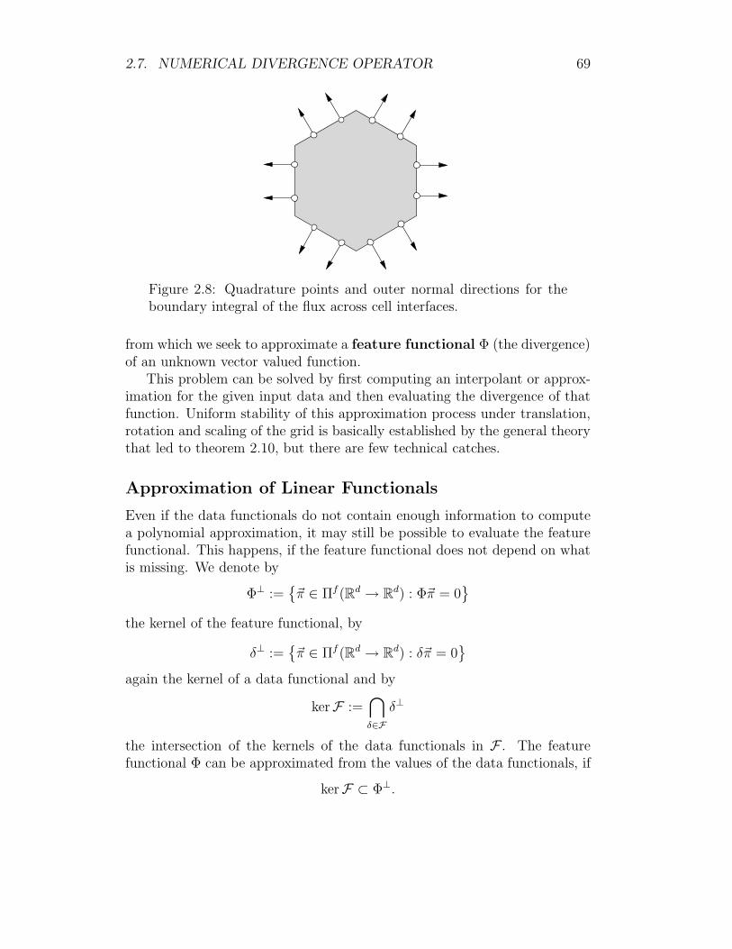
2.7. NUMERICAL DIVERGENCE OPERATOR 69

Figure 2.8: Quadrature points and outer normal directions for theboundary integral of the flux across cell interfaces.

from which we seek to approximate a feature functional Φ (the divergence)of an unknown vector valued function.

This problem can be solved by first computing an interpolant or approx-imation for the given input data and then evaluating the divergence of thatfunction. Uniform stability of this approximation process under translation,rotation and scaling of the grid is basically established by the general theorythat led to theorem 2.10, but there are few technical catches.

Approximation of Linear Functionals

Even if the data functionals do not contain enough information to computea polynomial approximation, it may still be possible to evaluate the featurefunctional. This happens, if the feature functional does not depend on whatis missing. We denote by

Φ⊥ :=~π ∈ Πf (Rd → R

d) : Φ~π = 0

the kernel of the feature functional, by

δ⊥ :=~π ∈ Πf (Rd → R

d) : δ~π = 0

again the kernel of a data functional and by

kerF :=⋂δ∈F

δ⊥

the intersection of the kernels of the data functionals in F . The featurefunctional Φ can be approximated from the values of the data functionals, if

kerF ⊂ Φ⊥.


An optimal choice of data functionals has maximal kerF , since we thenaccumulate exactly the information required for approximating the featurefunctional, like the construction of Gaussian quadrature formulae does forintegration. In this respect the finite volume method represents an exampleof an almost optimal choice. By the divergence theorem the cell average of afunctions divergence can be computed from the outer normal component ofthe function values on the cell boundary and the Gauss quadrature ensuresmaximum order of accuracy for each boundary part.

The proper polynomial trial space for the approximation of Φ from thefunctionals in F is

F⊥ := Πf(Rd → Rd)/ kerF .

We let Υ denote the closed convex hull of the evaluation points for the func-tionals in F and introduce the following norm on Π(Υ → R

d):

‖~π‖Υ,∞ := sup~x∈Υ

‖~π(~x)‖Rd

and the norm relative to F⊥:

‖~π‖F⊥ := inf~ω∈kerF

‖~π − ~ω‖Υ,∞ .

The functionals in F now have norm one, since

δ~π 6 ‖~π(~x)‖Rd 6 ‖~π‖Υ,∞

and equality holds, if ~π = ~n on all Υ. It should be noted that these constantfunctions are not in kerF , due to the form of the (new) data functionals.The condition of F can be defined as

condF := sup~π∈Πf (Rd→Rd)\kerF

‖~π‖F⊥

‖(δ~π)δ∈F‖∞.

Next we need to specify a reasonably large class of transformations of Rd

under which the condition of F is invariant. We do not attempt to covergeneral affine transformations, since stretching leads to a number of problemsconnected to the treatment of the evaluation directions: If we stretch figure2.8 horizontally, the hexagon would (seen from a distance) approximate arectangle and all outer normal vectors would tend to a horizental position.They would thus not approximate the outer normals of the rectangle.

For this reason we shall only consider similarity transformations of thegrid. The evaluation directions remain invariant under translations and scal-ing of the grid, but are rotated along with it. Invariance of the condition ofF under these transformations can now be established similar to lemma 2.7by considering the following transformations of ~π:


Figure 2.9: Stencil for approximating the feature functional at a cer-tain data location. It consists of evaluation points (white circles)and evaluation directions (arrows). Evaluation points with up to devaluation directions may coincide.

• ~π A−1 for translations and isotropic scaling operations A and

• A ~π A−1 for orthogonal transformations A of the grid.

If ~π is in kerF , then the transformation of ~π is in the kernel of the accordinglytransformed data functionals. The norm of the data functionals does notchange under the transformation. We may hence expect that the conditionof the vector valued approximation problem is uniformly bounded under thesekinds of transformations.

Next we consider again a least-squares approximation problem. We in-troduce on RF a scalar product

〈α; β〉RF := αtGβ

with a symmetric and positive definite Gram matrix G, the Euclidean G-norm

‖α‖G :=√

〈α; α〉RF

and solve the following problem: Find ~π ∈ F⊥ such that∥∥(δ~π − δ~g)δ∈F∥∥2

G→ min .

The Gram matrix G is again simply a diagonal matrix which provides geo-metric weighting in terms of powers of

‖~x − barycentre Υ‖Rd

diam Υ.


Choosing a basis

B = (~π1, . . . , ~πdimF⊥)

of F⊥ we obtain the matrix form ‖Aξ − θ‖2G → min of the least-squares

problem with

A := (δ~π)δ∈F ,~π∈B ∈ RF×B

θ := (δ~g)δ∈F ∈ RF .

The approximating vector valued polynomial is

Bξ =dimF⊥∑

k=1

ξk~πk

and the feature functional can be evaluated as

ΦBξ =dimF⊥∑

k=1

ξkΦ~πk.

We are ultimately interested in evaluating the feature functional, and notin the approximating polynomial as such. This now suggests computing avector of feature weights φ ∈ R

F which gives

ΦBξ = 〈φ; θ〉RF

by simply forming the scalar product of the vector of the feature weightswith the input data vector. Since we have

Aξ ≈ θ,

we would expect

ΦBξ ≈ 〈φ; Aξ〉RF .

This leads us to looking for φ as a solution of

ΦB ≈ φtGA.

The last relation is not overdetermined and can be solved exactly (A hasmaximal rank), but not necessarily uniquely. In fact, we have obtained thedual problem of the originial least-squares approximation problem: Findφ ∈ RF such that

φtGA = ΦB and ‖φ‖G → min . (2.21)


We observe that the dual problem is independent of the particular choiceof basis polynomials. Changing the basis amounts to multiplying the lastequation from the right with a regular R

B×B matrix and does not alter φ.The dual problem is most conveniently solved using the QU -decompositionof CA (as usual we denote the Cholesky decomposition of the Gram matrixby G = CtC)

CA = Q

(U0

)with an orthogonal matrix Q = Q−t ∈ RF×F and a regular upper triangularmatrix U ∈ R

B×B. We obtain

φt := ΦB (U−1|0)QtC−t. (2.22)

Lemma 2.13. The least-squares approximation to the feature functional Φobtained by evaluating the feature functional for a least-squares approxima-tion of the input data values is equivalent to taking the scalar product of thevector of feature weights obtained from the dual problem and the input datavector.

Proof. We need to show that

〈φ; θ〉RF = ΦBξ

for all θ ∈ RF . As ξ depends on θ via a least-squares problem, this isequivalent to

〈φ; θ〉RF = ΦB (U−1|0)QtCθ.

The latter is indeed the case, since we have by the definition (2.22) of φt

〈φ; θ〉RF = φtGθ = ΦB (U−1|0)QtC−tCtCθ.

Based on lemma 2.13 we can precompute the required vectors of featureweights during the preprocessing stage. They only have to be recomputed,if the grid is changed. Furthermore, the tasks of generating a divergence for-mula and the actual divergence computation are now completely separated.It is convenient to store φtG = ΦB (U−1|0)QtC.


Figure 2.10: Two kinds of divergence stencils. The evaluation direc-tions are parallel to the edges joining the dark vertices (barycentres ofdata locations). In the right part two evaluation points (white circles)per edge are considered. They are chosen on the mid-perpendicularof each edge, at a fixed portion (one fifth) of the edges length fromthe midpoint. Each evaluation point is affiliated to two dark verticesand the evaluation directions for both dark vertices are collinear.

The Divergence Functional

Choosing the basis B of F⊥ as functions of

~x − barycentre Υ

diam Υ

we obtain for the divergence of the basis functions:

divB =1

diam Υ

(div ~π

(~x − barycentre Υ

diam Υ

))~π∈B

.

While the condition of the interpolation matrix A := (δ~π)δ∈F ,~π∈B can bearranged to be invariant under scaling of the grid, we loose one order ofaccuracy via the right hand side of the dual problem (2.21), as should be ex-pected for first derivatives. For a first order approximation to the divergenceoperator we choose as in [AHS99]

Π1(Υ → Rd)

as trial space. It has dim Π1(Υ → Rd) = d(d+1). If all evaluation directionsall lead radially away from the barycentre of the data location for which thedivergence is to be computed (see figure 2.10 left), then the “eddy” functions(taking the barycentre as the origin)

~x 7→ (~x · ~ej)~ek − (~x · ~ek)~ej for j 6= k ∈ 1, . . . , dare in kerF . For this kind of stencil we can (and indeed have to) reducethe dimension of the trial space by d− 1, the number of independent “eddy”


functions. The reduced trial space has dimension d2 + 1. If there are notenough neighbours available in the collocation grid for interpolation, one hastwo options:

• One might insert extra edges to increase the number of neighbours or

• increase the number of evaluation points (figure 2.10 right) or evalua-tion directions without changing the number of neighbours.

It should be noted that this problem is not present for the finite volumemethod, as the boundary integral can be formally approximated with evenone evaluation point.

One extreme case of divergence stencil selection would be the choice ofd (linearly independent) evaluation directions per d coinciding evaluationpoints. The vector of feature weights will then contain d weights for suchan evaluation point: one per direction. These weights depend linearly onthe evaluation directions for a point. Consequently there exists a basis ofevaluation directions for which d− 1 of the weights vanish. For the directionof the non vanishing weight a numerical flux function should be computedand used as input datum for the divergence formula.

It is, however, not clear, whether a global choice of evaluation pointsand evaluation directions for collocation schemes is possible, such that thereis for each evaluation point only one non-zero weight and the evaluationdirections for the non-zero weights for the adjacent data locations are linearlydependent. In order to keep the cost of geometric preprocessing in reasonablebounds, we simply choose evaluation points and directions according to theedges, as in figure 2.10.

Figure 2.11: Part of divergence stencils for boundary edges. No eval-uation point outside the computational domain is chosen. Insteadwe choose further points (white circles) on the boundary edge itselfand outer normals as evaluation directions. The left two evaluationpoints on the boundary are affiliated to the left dark vertex, the rightones to the right dark vertex. The upper evaluation point is affiliatedto both dark vertices.


Higher Order Divergence

A higher order polynomial approximation requires substantially more data,

dim Πf(Rd → Rd) = d

(d + f

f

).

Using many levels of neighbours for this computation gave unsatisfactory re-sults and does not seem plausible in terms of the underlying physical trans-port mechanism. We therefore suggest a higher order divergence formulabased on the quasi linear form of the conservation law

div(F u) =∂F

∂u∇u

in smooth regions of the flow. The two divergence formulae for first andhigher order approximation can be blended by a simple limiting strategy.

If u is locally C1 about a data location, then the two values of u consideredfor an evaluation point differ aboutO(h) and so do the values of ∇u computedfrom the reconstruction on the cell itself and its neighbours. The followingsmoothness indicator

w :=∑

(ui − uo)2 + ‖∇ui −∇uo‖2

where the sum is taken over all evaluation points will thus be of order O(h2)for smooth parts of the flow and large for regions where u fails to be C1.Thus (

1 − w2

h2

)∇·(F u) +

w2

h2

∂F

∂u∇u

where ∇· represents a stable first order approximation could be used as anasymptotically high order divergence formula. In our numerical experiments,however, this switching strategy did not alter the solutions noticably.

2.8 The CFL Condition

For a one dimensional scheme of Godunov type the waves entering a cell oflength h from one end should not be allowed to travel across the whole celland leave it at the opposite end within a single time step. This leads to atime step constraint of

∆t <h

LF.

2.8. THE CFL CONDITION 77

In several space dimensions waves entering a cell near a corner across differentfaces would start interacting very early, but numerical experience indicatesthat this is not a principal source of trouble. Let us therefore focus onthe issue of information propagation in the scheme. For a scalar equationinformation clearly travels along characteristics at speed LF . If the physicallyrelevant part of the numerical scheme, this is the discrete divergence operatorfor the time step, does not process all of the physically relevant information,then arbitrarily changing the initial values outside the numerical domainof dependence changes the behaviour of the exact solution, but leaves theapproximation produced by the scheme unchanged. The scheme can thereforenot converge to the correct solution. In fact, a time step chosen too largeoften manifests itself in numerical instability. Let us clarify the point for theclassical Lax-Friedrichs scheme on a grid of uniform mesh size h in one spacedimension:

TS(u, t, ∆t)(xk) =

u(t, xk+1) + u(t, xk−1)

2− ∆t

2h[F (u(t, xk+1)) − F (u(t, xk−1))]

Here the numerical signal velocity is h/∆t, as information from neighbours toboth sides having distance h enters the numerical divergence approximation,whereas the physical signal velocity is the Lipschitz constant LF of the flux.We demand that the numerical signal velocity be greater than the physicalsignal velocity:

h

∆t> LF .

This reasoning, originally presented by Courant, Friedrichs and Levy in[CFL28], leads us to the following procedure for computing a legal time stepsize ∆t:

Estimate for each data functional δ a local Lipschitz constant LF of theflux function supplying δu as the argument and a local characteristic lengthh as half the diameter of the divergence stencil. Define with an arbitrarypositive constant CFL ∈ R>0:

∆t := CFLminδ∈Λ

h

LF.

The constant CFL is called the CFL number. Constraints of the time stepsize may be expressed as restrictions on CFL. For the Lax-Friedrichs scheme,for instance, we demand CFL < 1.


x

tnumerical domain of dependence

physical domain of dependence

data involved in time step

Figure 2.12: The CFL condition: Numerical and physical signal ve-locity.

For an implicit scheme the numerical signal velocity is infinite, as theimplicit time step will link events throughout the grid together. Implicitschemes have much less severe time step constraints in terms of stability andallow considerably larger time steps. These are, however still restricted bythe necessity to compute accurate approximations.

One might object that a scheme including substantially more than thephysically relevant information to compute the updates in a time step wouldfor reasons similar to those above fail to converge to the correct solution:changing the data outside the physical but within the numerical domainof dependence will change the numerical solution, while the exact solutionat a certain point remains unchanged. The major deception about this ar-gumentation is that it postulates propagation along characteristics for thenumerical scheme, too. However, the way the “extra” information is used bythe scheme is certainly subject to a consistency condition. It will probablyslow down the rate of convergence, but as long as the scheme remains stableand consistent not destroy it.

Chapter 3

The Euler Equations of GasDynamics

3.1 The Euler Flux Function

The Euler Equations represent the conservation of mass, momentum andenergy respectively. They describe the motion of a compressible liquid in theabsence of inner friction. In this respect they form a limit case of the systemof Navier-Stokes equations. We denote by ρ the density, ~v the transportvelocity, E the specific energy, i.e. energy per mass and by p the pressure.The flux function for the Euler equations reads

F = ρ

1~vE

~vt + p

0I~vt

(3.1)

(the middle line of equation (3.1) is a shorthand notation for d lines) withan equation of state which for an ideal gas takes the form

p = (κ − 1)ρ(E − 1

2‖~v‖2) . (3.2)

For an ideal diatomic gas the constant κ takes the value κ = 7/5 = 1.4. Wealso introduce the constant κ := κ − 1. The set S ⊂ R

s of valid physicalstates with s = d + 2 is restricted to ρ > 0 and p > 0. The system of theEuler equations now reads:

∂

∂t

ρρ~vρE

+ div

ρ

1~vE

~vt + p

0I~vt

= 0. (3.3)

79

80 CHAPTER 3. THE EULER EQUATIONS OF GAS DYNAMICS

The quantities differentiated with respect to time

u :=

ρρ~vρE

are called conservative variables: density (of mass), density of momentumand density of energy. We define the enthalpy H, the (unscaled) thermody-namic entropy Z and the speed of sound a as

H := E +p

ρ

Z := lnp

ρκ

a :=

√κp

ρ.

(3.4a)

The term “unscaled” indicates that we have omitted the specific heat capacityat constant volume from the definition of the thermodynamic entropy. Thethermodynamic entropy is a concave function. Compared to the discussionof the abstract entropy on page 18 this corresponds to a different sign con-vention, i.e. the thermodynamic entropy will increase across a discontinuity.The following relations are useful:

H = κE − 12κ ‖~v‖2

κH = a2 + 12κ ‖~v‖2

∇up = κ(

12‖~v‖2 , −~vt, 1

)∇uZ =

1

p

(12κ ‖~v‖2 − a2, −κ~vt, κ

)∇ua =

1

2ρa

(12κκ ‖~v‖2 − a2, −κκ~vt, κκ

).

(3.4b)

The index u to the nabla operator indicates that differentiation is performedwith respect to the conservative variables Along a fixed unit vector ~n ∈ R

d

we define

v~n := ~v · ~n.

After multiplication with this vector ~n equation (3.1) takes the form

F~n =

ρv~n

ρv~n~v + p~nρHv~n

(3.5)

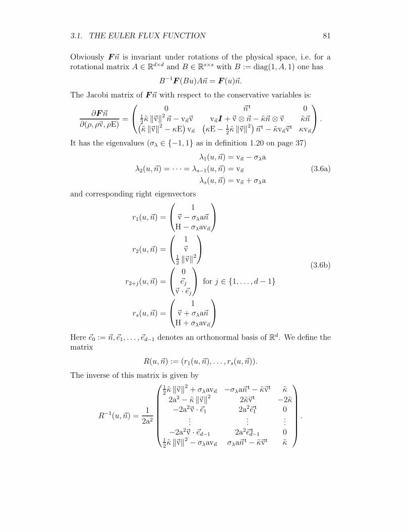
3.1. THE EULER FLUX FUNCTION 81

Obviously F~n is invariant under rotations of the physical space, i.e. for arotational matrix A ∈ R

d×d and B ∈ Rs×s with B := diag(1, A, 1) one has

B−1F (Bu)A~n = F (u)~n.

The Jacobi matrix of F~n with respect to the conservative variables is:

∂F~n

∂(ρ, ρ~v, ρE)=

0 ~nt 012κ ‖~v‖2 ~n − v~n~v v~nI +~v ⊗ ~n − κ~n ⊗~v κ~n(κ ‖~v‖2 − κE

)v~n

(κE − 1

2κ ‖~v‖2)~nt − κv~n~v

t κv~n

.

It has the eigenvalues (σλ ∈ −1, 1 as in definition 1.20 on page 37)

λ1(u, ~n) = v~n − σλa

λ2(u, ~n) = · · · = λs−1(u, ~n) = v~n

λs(u, ~n) = v~n + σλa

(3.6a)

and corresponding right eigenvectors

r1(u, ~n) =

1~v − σλa~nH − σλav~n

r2(u, ~n) =

1~v

12‖~v‖2

r2+j(u, ~n) =

0~ej

~v · ~ej

for j ∈ 1, . . . , d − 1

rs(u, ~n) =

1~v + σλa~nH + σλav~n

(3.6b)

Here ~e0 := ~n,~e1, . . . , ~ed−1 denotes an orthonormal basis of Rd. We define thematrix

R(u, ~n) := (r1(u, ~n), . . . , rs(u, ~n)).

The inverse of this matrix is given by

R−1(u, ~n) =1

2a2

12κ ‖~v‖2 + σλav~n −σλa~nt − κ~vt κ

2a2 − κ ‖~v‖2 2κ~vt −2κ−2a2~v · ~e1 2a2~e t

1 0...

......

−2a2~v · ~ed−1 2a2~e td−1 0

12κ ‖~v‖2 − σλav~n σλa~n

t − κ~vt κ

.


Linear independence of the right eigenvectors is therefore assured and wehave the following

Lemma 3.1. The Euler equations (3.3) are hyperbolic. In one space dimen-sion they are even strictly hyperbolic.

3.2 Riemann Invariants

The eigenvalues and eigenvectors originating from the Euler equations (3.3)are either genuinely nonlinear or linearly degenerate. Specifically:

Lemma 3.2. The eigenvalues λ1 and λs are genuinely nonlinear, λ2, . . . , λs−1

are linearly degenerate.

Proof. We consider first λ2 = · · · = λs−1 = v~n:

∇uv~n = ∇uλ2 = · · · = ∇uλs−1 =1

ρ

(−v~n, ~nt, 0)

(3.7)

is clearly orthogonal on r2, . . . , rs−1. For λs we have:

∇u(v~n + σλa) =1

ρ

(−v~n, ~nt, 0)

+ σλκκ

2ρa

(1

2‖~v‖2 − a2

κκ, −~vt, 1

)and

σλκκ

2ρa

(1

2‖~v‖2 − a2

κκ, −~vt, 1

) 1~v + σλa~nH + σλav~n

+

1

ρ

(−v~n, ~nt, 0) 1

~v + σλa~nH + σλav~n

= σλa

2ρ(κ + 1) 6= 0.

The eigenvalue λ1 takes the role of λs, if we reverse the ordering by changingthe sign of σλ.

The Riemann invariants corresponding to the eigenvalues are summarized intable 3.1 on page 83. Using the relations from equation (3.4b) they are easilyverified.

3.2. RIEMANN INVARIANTS 83

Ψ(1)1 = v~n + σλ

2

κa

λ1 = v~n − σλa Ψ(1+j)1 = ~v · ~ej for j ∈ 1, . . . , d − 1

Ψ(s−1)1 = Z

Ψ(1)2 = v~n

λ2 = v~n Ψ(1+j)2 = ~v · ~ej for j ∈ 1, . . . , d − 1

Ψ(s−1)2 = p

Ψ(1)k = v~n

λk = v~n Ψ(1+j)k = ~v · ~ej for j ∈ 1, . . . , d − 1 \ k − 2

for k ∈ 3, . . . , s − 1 Ψ(k−1)k = ρ

Ψ(s−1)k = p

Ψ(1)s = v~n − σλ

2

κa

λs = v~n + σλa Ψ(1+j)s = ~v · ~ej for j ∈ 1, . . . , d − 1

Ψ(s−1)s = Z

Table 3.1: Riemann invariants for the Euler equations


3.3 Jump Relations

Certain properties of the solution to the Riemann problem for the Eulerequations can be deduced directly from the directed flux of equation (3.5).Since each of the conservative variables is conserved in its own right, wegather from the Rankine-Hugoniot jump condition (1.15) for a discontinuityaligned with a hyperplane orthogonal to a fixed unit vector ~n ∈ Rd andmoving at velocity ~ν = ‖~ν‖~n and ~e1, . . . , ~ed−1 orthogonal to ~n:

ρ(l)(v

(l)~n − ‖~ν‖ ) = ρ(r)

(v

(r)~n − ‖~ν‖ ) (3.8a)

ρ(l)(v

(l)~n − ‖~ν‖ )2 + p(l) = ρ(r)

(v

(r)~n − ‖~ν‖ )2 + p(r) (3.8b)

ρ(l)(v

(l)~n − ‖~ν‖ )~v(l) · ~ej = ρ(r)

(v

(r)~n − ‖~ν‖ )~v(r) · ~ej (3.8c)

ρ(l)(v

(l)~n − ‖~ν‖ )H(l) = ρ(r)

(v

(r)~n − ‖~ν‖ )H(r). (3.8d)

If v(l)~n = ‖~ν‖, then by equation (3.8a) v

(r)~n = ‖~ν‖ and by (3.8b) p(l) = p(r).

This situation is a contact discontinuity. Since the velocity components or-thogonal to the hyperplane equal the speed of the discontinuity, no fluidparticle can pass.

If v(l)~n 6= ‖~ν‖, then by equation (3.8a) v

(r)~n 6= ‖~ν‖ and by equation (3.8c)

~v(l) · ~ej = ~v(r) · ~ej . Similarly by equation (3.8d) H(l) = H(r). Let us nowassume that v

(l)~n 6= v

(r)~n , since otherwise there is really no discontinuity at all.

H(l) − 1

2

(~v(l) · ~ej

)2= H(r) − 1

2(~v(r) · ~ej)

2

gives the following definition of a∗ in terms of either left or right state:

(a(l))2

κ − 1+

1

2

(v

(l)~n − ‖~ν‖ )2 =

(a(r))2

κ − 1+

1

2

(v

(r)~n − ‖~ν‖ )2 =:

1

2

κ + 1

κ − 1(a∗)2. (3.9)

Dividing equation (3.8b) by equation (3.8a)

v(l)~n − ‖~ν‖ +

p(l)

ρ(l)(v

(l)~n − ‖~ν‖ ) = v

(r)~n − ‖~ν‖ +

p(r)

ρ(r)(v

(r)~n − ‖~ν‖ )

and therefore

v(l)~n − v

(r)~n =

(a(r))2

κ(v

(r)~n − ‖~ν‖ ) −

(a(l))2

κ(v

(l)~n − ‖~ν‖ ) .

Use of equation (3.9) to eliminate(a(l))2

and(a(r))2

finally yields(v

(l)~n − ‖~ν‖ )(v(r)

~n − ‖~ν‖ ) = (a∗)2.

3.4. NUMERICAL FLUX FUNCTIONS 85

Introducing the Mach numbers (relative to ‖~ν‖)

Mal :=v

(l)~n − ‖~ν‖

a(l)Mar :=

v(r)~n − ‖~ν‖

a(r)

Ma∗l :=v

(l)~n − ‖~ν‖

a∗Ma∗

r :=v

(r)~n − ‖~ν‖

a∗

we conclude

Ma∗l Ma∗r = 1 (3.10a)

and from equation (3.9) (Ma refers to either Mal or Mar, Ma∗ to Ma∗l or Ma∗r)(Ma∗

)2=

(κ + 1)Ma2

(κ − 1)Ma2 + 2. (3.10b)

From equation (3.8a) we now infer the jump relation for the density

ρ(l)

ρ(r)=

Ma∗rMa∗l

=(Ma∗r

)2=

(κ + 1)(Mar

)2(κ − 1)

(Mar

)2+ 2

, (3.11a)

for the pressure from equation (3.8b)

p(l) − p(r) = ρ(l)(v

(l)~n − ‖~ν‖ )2 − ρ(r)

(v

(r)~n − ‖~ν‖ )2

= ρ(r)(v

(r)~n − ‖~ν‖ )(v(l)

~n − v(r)~n

)by equation (3.8a)

= (a∗)2ρ(r)(1 − (Ma∗r

)2)and

p(l)

p(r)= 1 +

2κ

κ + 1

(1 − (Mar

)2). (3.11b)

3.4 Numerical Flux Functions

For the numerical flux function HOS of Osher and Solomon the integrationin equation (1.38) is simplified considerably by the fact that s−2 eigenvaluesof the Jacobi matrix of the directed Euler flux in equation (3.5) are linearlydegenerate. Furthermore, these s − 2 eigenvalues are equal. The remainingtwo eigenvalues are genuinely nonlinear, one of them is greater and the othersmaller than the degenerate ones.

The path components whose tangents are the linearly degenerate eigen-vectors do not contain any sonic points, and the sum over the flux integrals


along these components reduces to the difference of the fluxes for just twointermediate states (equation (3.12d) contains the definition of v

(m)~n ):

s−1∑k=2

∫Γk

(∂F~n

∂u

∣∣∣∣u

)+

du =

F (es−1)~n − F (s2)~n if v

(m)~n > 0

0 if v(m)~n 6 0.

Therefore we need to determine two intermediate states u(1) = s2 and u(2) =es−1. Using superscripts (l), (1), (2) and (r) to indicate affiliation to ul, u(1),u(2) and ur respectively, we infer for Γ1 from the Riemann invariants listedin table 3.1 on page 83

v(1)~n + σλ

2

κa(1) = v

(l)~n + σλ

2

κa(l) =: Ψ(l) (3.12a)

~v(1) · ~ej = ~v(l) · ~ej for j ∈ 1, . . . , d − 1 (3.12b)

Z(1) = Z(l), (3.12c)

for the middle paths Γ2, . . . , Γs−1 (ρ and ~v · ~ej are not needed)

v(1)~n = v

(2)~n =: v

(m)~n (3.12d)

p(1) = p(2) (3.12e)

and for the final path component Γs

v(2)~n − σλ

2

κa(2) = v

(r)~n − σλ

2

κa(r) =: Ψ(r) (3.12f)

~v(2) · ~ej = ~v(r) · ~ej for j ∈ 1, . . . , d − 1 (3.12g)

Z(2) = Z(r). (3.12h)

From the definition of Z we infer

κκ exp(Z) = p−κa2κ and a =√

κpκ/κ exp

(Z

2κ

).

Equations (3.12e), (3.12c) and (3.12h) now imply

a(2)

a(1)= exp

(Z(2) − Z(1)

2κ

)= exp

(Z(r) − Z(l)

2κ

)=: α. (3.12i)

Together with equation (3.12a), its counterpart (3.12f) and equation (3.12d)we obtain from equation (3.12i) a system of three linear equations

v(m)~n + σλ

2

κa(1) = Ψ(l)

v(m)~n − σλ

2

κa(2) = Ψ(r)

a(2) = αa(1)

3.4. NUMERICAL FLUX FUNCTIONS 87

which gives us

a(1) = σλκ

2

Ψ(l) − Ψ(r)

1 + α

a(2) = σλακ

2

Ψ(l) − Ψ(r)

1 + α

v(m)~n =

αΨ(l) + Ψ(r)

1 + α.

This solution is physically meaningful, only if σλ(Ψ(l) − Ψ(r)) > 0. Having

thus computed the velocity component parallel to ~n and the speeds of soundfor the intermediate states, we need to decide whether Γ1 and Γs containsonic points. That is the case for Γ1, if and only if(

v(l)~n − σλa

(l))(

v(m)~n − σλa

(1))

< 0

and for Γs, if and only if(v

(r)~n + σλa

(r))(

v(m)~n + σλa

(2))

< 0.

A sonic point nk is in either case characterized by λk(nk) = 0 (k ∈ 1, s).We denote by v∗ the velocity component parallel to ~n and by a∗ the speed ofsound for the sonic point. A superscript (l) refers to Γ1, (r) to Γs. Togetherwith equations (3.12a) and (3.12f) we obtain the following linear equations:

0 = v(l)∗ − σλa

(l)∗ 0 = v(r)

∗ + σλa(r)∗

Ψ(l) = v(l)∗ + σλ

2

κa(l)∗ Ψ(r) = v(r)

∗ − σλ2

κa(r)∗ .

They admit the solutions (σλ2 = 1)

v(l)∗ =

κ − 1

κ + 1Ψ(l) v(r)

∗ =κ − 1

κ + 1Ψ(r)

a(l)∗ = σλ

κ − 1

κ + 1Ψ(l) a(r)

∗ = −σλκ − 1

κ + 1Ψ(r).

By equation (3.12c) the entropy is constant on Γ1, by its companion (3.12h)on Γs. The velocity components orthogonal to ~n are similarly constant onΓ1 by equation (3.12b) and by equation (3.12g) on Γs. At this stage we havethus at our disposal speed of sound, transport velocity and entropy for anyintermediate or sonic state. These variables (a,~v, Z) are called character-istic variables. In order to evaluate equation (3.5) for a certain state we


compute density, pressure and enthalpy as follows:

ρ = exp

(ln(a2/κ) − Z

κ

)p =

a2ρ

κ

H =a2

κ+

1

2‖~v‖2 .

We may optimize the computation of ‖~v‖2, if we observe that for two vectors~ν and ~ν ′ differing only in their components parallel to ~n

‖~ν ′‖2= ‖~ν‖2 − (~ν~n)2 + (~ν ′

~n)2.

Evaluation of the integral in equation (1.38) is now straightforward. Thethesis of Spekreijse [Spe87] and the book by Toro [Tor97] contain tableslisting the explicit expressions for the flux function of Osher and Solomon inthe case of the Euler equations. We do not reproduce those tables here.

3.5 Boundary Conditions

We use the following two kinds of boundary conditions:

• fixed wall and

• moving shock.

The fixed wall boundary condition is characterized by the fact that no par-ticle can leave or enter across this part of the boundary. Consequently thevelocity component orthogonal to the boundary vanishes. Enforcing v~n = 0in equation (3.5) gives:

B =

0p~n0

. (3.13)

The moving shock boundary condition simulates the movement of a super-sonic shock along the boundary. The shock is represented by a hyperplanewith normal ~n separating two states ul and ur, such that ~n points from theregion of ul to that of ur. One has to specify the normal ~n to the hyperplane,the velocity ~ν = (~ν · ~n)~n at which the hyperplane shall move and the stateto the right of the hyperplane ur. The state ul to the left of the hyperplanecan then be computed in terms of the primitive variables (ρ,~v, p) usingequations (3.11). The outer state is either ul or ur depending on t and ~x,and an approximate Riemann problem can be solved in the usual fashion.

Chapter 4

Collocation Schemes

In this chapter we sketch some of our early attempts at developing a colloca-tion method for unstructured grids. These were based on the classical Lax-Friedrichs scheme and isotropic regularization of the solution with a Laplaceterm. We found these too dissipative and considered anisotropic regular-ization instead. One such method that works quite well on Cartesian gridsuses a digital filtering strategy at local extrema. In the unstructured caseusing a recovery procedure as a means of analyzing the local data and thedownhill transport mechanism immanent in numerical flux functions proveda cheap and superior alternative. We furnish some numerical examples todemonstrate the capabilities of such a scheme.

4.1 The Lax-Friedrichs Scheme

Cartesian Grids

The second order central finite difference scheme on a grid of constant meshsize h in one space dimension

TS(u, t, ∆t)(xk) = u(t, xk) − ∆t

2h[F (u(t, xk+1)) − F (u(t, xk−1))] (4.1)

is known to be unstable. This is easily seen by a von Neumann error analysisconsidering a linear flux function.

The von Neumann error analysis considers the evolution of a spatiallyperiodic disturbation of the data for a linear equation, by looking at eachterm of its Fourier expansion separately. If u has the spatial period L, then

89

90 CHAPTER 4. COLLOCATION SCHEMES

its Fourier expansion can at least formally be written as

u(j∆t, kh) =∑J∈Z

∑K∈Z

αJ,KξjJ exp

(2πiKkh

L

)where αJ,K are the Fourier coefficients and ξJ ∈ C is the expansion in time.Suppressing the indices a single Fourier term now has the form

ξj exp(iαk) with α ∈ R. (4.2)

With the linear flux F (u) = au (a ∈ R fixed) we infer

ξj+1 exp(iαk) = ξj exp(iαk) − a∆t

2h

[ξj exp(iα(k + 1)) − ξj exp(iα(k − 1))

]and hence

ξ = 1 − a∆t

2h[exp(iα) − exp(−iα)]

= 1 − ia∆t

hsin(α)

|ξ|2 = 1 +

(a∆t

hsin(α)

)2

> 1.

The amplitude of each error mode therefore increases exponentially in timewhich is precisely the alleged instability. The classic Lax-Friedrichs schemeremoves this instability by replacing the term u(t, xk) on the right hand sideof equation (4.1) with the average of u(t, xk+1) and u(t, xk−1):

TS(u, t, ∆t)(xk)

=u(t, xk+1) + u(t, xk−1)

2− ∆t

2h

[F (u(t, xk+1)) − F (u(t, xk−1))

]= u(t, xk) − ∆t

2h

[(F (u(t, xk+1)) +

h

∆t(u(t, xk) − u(t, xk+1))

)−(

F (u(t, xk−1)) +h

∆t(u(t, xk−1) − u(t, xk))

)]. (4.3)

A von Neumann error analysis for the linearized version of equation (4.3)yields

ξj+1 exp(iαk) = ξj exp(iα(k + 1)) + exp(iα(k − 1))

2

− a∆t

2h

[ξj exp(iα(k + 1)) − ξj exp(iα(k − 1))

]

4.1. THE LAX-FRIEDRICHS SCHEME 91

and thus

ξ = cos(α) − ia∆t

hsin(α)

|ξ|2 = cos2(α) +

[a∆t

hsin(α)

]2

= 1 +

[(a∆t

h

)2

− 1

]sin2(α)

which is less than one, if and only if

∆t <h

|a| .

From this point of view the CFL time step constraint [CFL28] appears asa condition ensuring exponential decay in time of spatially periodic errormodes. If we substitute h/∆t = LF /CFL in equation (4.3) and then dropthis occurence of CFL, we get back to the numerical Lax-Friedrichs fluxfunction:

HLF(u(t, xk), u(t, xk+1), +1) + HLF(u(t, xk), u(t, xk−1),−1)

≈ 1

2

(F (u(t, xk)) + F (u(t, xk+1)) +

h

∆t(u(t, xk) − u(t, xk+1))

)− 1

2

(F (u(t, xk−1)) + F (u(t, xk)) +

h

∆t(u(t, xk−1) − u(t, xk))

)This allows us to interprete the Lax-Friedrichs scheme as a finite volumescheme with piecewise constant reconstruction on cells of length h centeredabout each grid point xk. The Lax-Friedrichs scheme of equation (4.3) has alocal truncation error

L∆t(t, x) :=1

∆t[TS(u, t, ∆t)(x) − u(t + ∆t, x)]

that is linear, i.e. assuming smoothness and replacing u with its Taylor ex-pansion we obtain for the Lax-Friedrichs scheme L∆t = O(∆t). However, forthe modified equation

∂

∂tu + a

∂

∂xu = b

∂2

∂x2u (4.4a)

with

b :=∆t

2

(h2

(∆t)2− a2

)(4.4b)


the local truncation error is quadratic and the CFL restriction ∆t < h/ |a|implies that we are not simulating an ill-posed backward heat transport equa-tion. In smooth regions of the flow we obtain from equations (4.4)

∂2

∂t2u − a2 ∂2

∂x2u = b

(∂3

∂x2∂tu − a

∂3

∂x3u

)and

L∆t(t, x) =

(h2

2∆t− a2∆t

2− b

)∂2

∂x2u

+b∆t

2

(∂3

∂x2∂tu − a

∂3

∂x3u

)+ O((∆t)2)

With the choice of b of (4.4b) we have indeed L∆t = O((∆t)2). We nowseek to stabilize a central scheme on smoothly, but otherwise arbitrarilyscattered collocation points by adding diffusion in the spirit of the classicalLax-Friedrich scheme.

Unstructured Grids

We noted in [AFHS] that the amount of artificial diffusion in equations (4.4)depends nonlinearly on the local scale h. The time step size is determinedessentially by the smallest h in the grid and leads to unacceptable high dif-fusion in regions where the grid is coarse. Furthermore, if the CFL numberis halved, the diffusion per time step approximately doubles:

b =∆t

2

(1

CFL2 − 1

)a2.

To render diffusion independent of the CFL number we use a discrete dissi-pative model proportional to the chosen CFL number (and drop the −1):

CFL∆t

2

h2

(∆t)2.

We still need to define a “typical” scale h for each stencil. To this end weintroduce the local scale

hSΣ:=

diam ΣS2

and the global scale

hG := minΣ∈G

hΣ.

4.1. THE LAX-FRIEDRICHS SCHEME 93

The dissipative model can now be stated as

b := CFL∆t

2

hSΣhG

(∆t)2.

In our calculations we also replaced the division by two with a division byfour. Thus the modified diffusive equation we simulated was

∂

∂tu + div

(F u − CFL

∆t

4

hSΣhG

(∆t)2∇u

)= 0.

The evaluation points were chosen to be all collocation points in a centralstencil and two evaluation directions per evaluation point were used, i.e. weincorporated the full vector valued flux as obtained by computing the fluxfunction for the collocation point value of u, no reconstruction procedure wasapplied.

Figure 4.1: Solutions to the Burgers equation generated with theartificial diffusion model on the unit square [0, 1]2 ⊂ R2. Left ini-tial condition, middle 2013 points and right 7889 points. The simu-lated equation is in either case F (u) = u2(1, 1)t and the final time isT = 0.4. The initial condition consists in a Gauss bell shaped func-tion on a circle of radius 0.25 centered about (0.3, 0.3) with height 1.Riemann problems with outer state u = 0 are solved on the bound-ary. The upper parts of the bell are advected faster than the lowerparts and start to overtake at some point. At this stage a disconti-nuity is formed. On finer grids the dissipative effect decreases, butthe artificial diffusion necessary for stabilizing the scheme makes thesolutions too dissipative.

As an alternative we investigated a filtering strategy in the spirit of[ELS89]. Since numerical instability manifests itself in the generation ofnoise, i.e. extrema, we checked for local extrema after each time step and ap-plied a local smoothing procedure. If a local extremum had been generated


at a data location Σ, we computed the average of the data functional valueson a stencil consisting of Σ and its neighbours

avgS u :=1

cardS∑Θ∈S

δΣu

and then scaled the data functional values towards their average by replacingthe stored value of δΘu with

αδΘu + (1 − α) avgS u

for each Θ ∈ S. Choosing α ≈ 0.9 proved sufficient to stabilize the scheme,but gave a rather noisy solution, smaller values would diminish the noise,but increase diffusive smearing.

4.2 Upwinding Schemes

Anisotropic data dependent diffusion can also very efficiently be incorpo-rated into the scheme via numerical flux functions. It proved superior toour attempts of isotropic regularization without explicit reconstruction step.It should be noted that anisotropic regularization necessarily involves somekind of data analysis and that linear or higher order reconstruction can beregarded as a means of analyzing the local data. Let us illustrate this ideavery loosely: The integral formulation of a conservation law with a diffusiveterm reads

d

dt

∫Σ

u dV = −∫

∂Σ

(F u − b∇u)~n do. (4.5)

If we replace ∇u~n with a suitable difference quotient

∇u~n ≈ u(~xΣ) − u(~x′Σ)

‖~xΣ − ~x′Σ‖

where ~xΣ and ~x′Σ represent two points inside and outside the cell Σ respec-

tively on a line orthogonal to ∂Σ with

‖~xΣ − ~x′Σ‖ ≈ h,

we can interprete a numerical flux function H as an approximation to thediffusive flux of equation (4.5) with b suitably chosen. The numerical flux(ui and uo are again the inner and outer limit at the cell boundary)

H(ui, uo, ~n) =F (ui) + F (uo)

2~n + A

ui − uo

2

4.2. UPWINDING SCHEMES 95

with a suitable upwinding term A ∈ [0, LF ] approximates the integrand in(4.5), if we identify (F u)~n with (F (ui) + F (uo))~n/2 and observe

Aui − uo

2= A

‖~xΣ − ~x′Σ‖

2

ui − uo

u(~xΣ) − u(~x′Σ)

u(~xΣ) − u(~x′Σ)

‖~xΣ − ~x′Σ‖

≈ A‖~xΣ − ~x′

Σ‖2

ui − uo

u(~xΣ) − u(~x′Σ)︸︷︷︸

=:b

∇u~n.

The reconstruction process of degree q will generally ensure that

ui − uo

u(~xΣ) − u(~x′Σ)

=

1 + O(h) > 0 at discontinuities

O(hq) in smooth regions of the flow.

The artificial diffusion contributed by approximating the integrand in equa-tion (4.5) with a numerical flux function therefore decreases very rapidly insmooth regions of the flow. Near discontinuities it constitutes the requireddownhill transport necessary to ensure proper physical transport. The argu-mentation is of course flawed, if u(~xΣ) = u(~x′

Σ).The results of the numerical flux computation are used as input data for

approximating the divergence functional. In this context we use only oneevaluation direction per evaluation point.

Figure 4.2: Solutions to the Burgers equation generated with theupwinding method. Middle 2013 points and right 7889 points. Thesetup is identical to figure 4.1.

Choice of Data Locations

Because of the diffusive effect immanent in the solution to local Riemannproblems, too, positive divergence formulae have to be used: the numericalfluxes directed away from a data location should have a positive weight in the


formula for approximating the flux divergence at that point. Otherwise onewould locally simulate the behaviour of a “backward heat transport equation”and suffer numerical instability. We have still some freedom in the exactchoice of the collocation functionals which we now use to obtain such positiveformulae:

As collocation functionals we choose the average of the pointwisecollocation at each evaluation point in the divergence stencil.

The positivity of a weight w is checked in the following way: Letting ~x denotean evaluation point in the divergence stencil, ~n the evaluation direction forthis point and ~x0 the average of the evaluation points we demand

~n · (~x − ~x0) sign(w) > 0. (4.6)

Up to linear reconstruction this choice of the collocation functionals is equiv-alent to collocation about the barycentre of the divergence stencil.

4.3 Numerical Experiments

Finally we present numerical results for the Euler equations obtained withthe upwind collocation method.

2D Shock Tube for the Euler Equations

In this section we present results for the two dimensional shock tube problemwith parameters suggested by Lax and Sod. The shock tube has length oneand initially a diaphragm at x = 0.5 separating gas in different states to itsleft and right. At time t0 = 0 the diaphragm is removed and the gas startsto mix.

Lax (T = 0.1445) Sod (T = 0.18)left right left right

ρ 0.445 0.5 1 0.125~v 0.698~e0 0 0 0p 3.528 0.571 1 0.1

Table 4.1: Initial configuration at t0 = 0 for Lax and Sod shock tubeproblems.

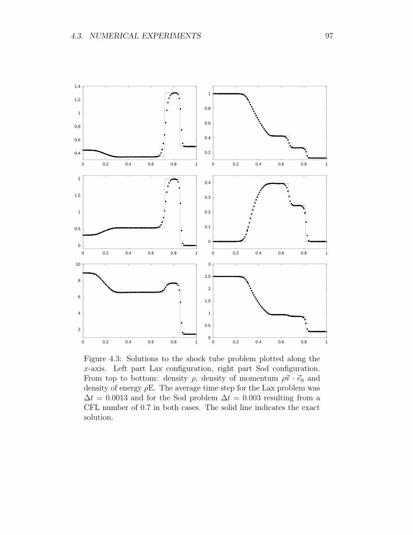
4.3. NUMERICAL EXPERIMENTS 97

0.4

0.6

0.8

1

1.2

1.4

0 0.2 0.4 0.6 0.8 1

0.2

0.4

0.6

0.8

1

0 0.2 0.4 0.6 0.8 1

0

0.5

1

1.5

2

0 0.2 0.4 0.6 0.8 1

0

0.1

0.2

0.3

0.4

0 0.2 0.4 0.6 0.8 1

2

4

6

8

10

0 0.2 0.4 0.6 0.8 10

0.5

1

1.5

2

2.5

3

0 0.2 0.4 0.6 0.8 1

Figure 4.3: Solutions to the shock tube problem plotted along thex-axis. Left part Lax configuration, right part Sod configuration.From top to bottom: density ρ, density of momentum ρ~v · ~e0 anddensity of energy ρE. The average time step for the Lax problem was∆t = 0.0013 and for the Sod problem ∆t = 0.003 resulting from aCFL number of 0.7 in both cases. The solid line indicates the exactsolution.


The computational grid we used covered the region [0, 1]× [−0.05, 0.05] ⊂R

2. It consisted of 1309 points which corresponds to roughly 100 pointsspread along the x-axis. We show the results in figure 4.3. The jump of thedensity for the contact disontinuity in the Lax case is smeared over someten cells, in the Sod case over six cells. This is comparable to the resultspresented by Botta [Bot95] for the van Leer limiter.

On the top and bottom part of the grids margin we applied the fixedwall boundary condition and supplied the constant states from the initialcondition on the left and right part of the boundary. No particular measureswere taken to keep the flow inside the tube one dimensional. We show theiso-lines of the density in figures 4.4 and 4.5.

Figure 4.4: Iso-lines of the density for the Lax shock tube problem.

Figure 4.5: Iso-lines of the density for the Sod shock tube problem.

Double Mach Reflection

The double Mach reflection of a strong shock can be realized experimentallyby driving a shock down a tube that contains a wedge. Our configurationfollows the one presented in [WC84]: a fast planar shock making an angle of60 with the x-axis meets a fixed wall. This setup is commonly regarded asa challenging test case.

The computational domain we used was trapezoidal with corners at (0, 0),(3, 0), (3, 3/4) and (

√3/4, 3/4). The fixed wall lies at the bottom of the com-

putational domain and stretches from x = 1/6 to the right. The undisturbedresting gas to the right of the shock has density ρ = 1.4 and pressure p = 1.Its speed of sound therefore is a = 1. The shock moves at Mach 10, its veloc-ity vector is (5

√3,−5). Initially (t = 0) the shock front touches the leftmost

point of the wall.All parts of the domains boundary that are not formed by the wall are

treated with the moving shock boundary condition. Based on the prescribedvalues for the shocks propagation speed and the state of the gas ahead of the

4.3. NUMERICAL EXPERIMENTS 99

shock the state of the gas behind the shock can be computed using the jumprelations for the Euler equations. On the boundary the appropriate one ofthe two states is used as outer state and a Riemann problem can be solvedin the usual way. In figure 4.6 we show the iso-lines of the computed solutionfor three subsequently refined grids.

Figure 4.6: Iso-lines of density for the double Mach reflection at T =0.2. Top 25831 points, middle 102629 points and bottom 409037points. The bottom line of each picture indicates the position of thewall.

Appendix A

Measure of an equilaterald-dimensional simplex

Lemma A.1. The Jordan measure (volume) of an equilateral simplex Σ ofdiameter a in d dimensions is

|Σ| =1

d!√

d + 1

(a√2

)d

.

Proof. The simplex Fd(l) :=

(x1, . . . , xd) ∈ Rd : xk > 0 and∑d

k=1 xk 6 l

has volume

|Fd(l)| =ld

d!

as is easily seen by induction: For d = 1 one has |F1(l)| = l and for d > 2|Fd(l)| = |Fd−1(l)| l/d by the “base times height divided by d” rule. All edgesof the sub-simplex Σd−1(l) of Fd(l) formed by all vertices save ~v = 0 havelength a = l

√2 and this is also the diameter of Σd−1(l). The height of Fd(l)

on this sub simplex is formed by the vector (1, . . . , 1)l/d ∈ Rd which haslength l/

√d. Now

|Σd−1(l)| =d |Fd(l)|l/√

d=

ld−1

(d − 1)!√

d

and

|Σd(l)| =ld

d!√

d + 1=

ad

d!√

2d(d + 1).

101

102 APPENDIX A. MEASURE OF D-DIMENSIONAL SIMPLEX

Lemma A.2. For the simplex Σ of the preceding lemma we have

|Σ||∂Σ| diam(Σ)

=1

d(d + 1)

√d

2(d + 1).

Proof. Σ = Σd(l) has d + 1 faces Σd−1(l) and therefore

|Σ||∂Σ| diam(Σ)

=

1d!√

d+1

(a√2

)d

d+1(d−1)!

√d

(a√2

)d−1

a=

1

d(d + 1)

√d

2(d + 1).

Appendix B

List of Symbols

A closure of the set Aco A closed convex hull of A|x| absolute value of x ∈ R

|X| absolute value of the diagonalizable matrix X ∈ Rn×n

|Σ| Jordan measure (volume) of Σ ⊂ Rd

(A → B), BA mappings from A to B‖·‖ Euclidean norm in Rd

‖·‖G Euclidean G-norm in Rn

‖·‖∞ maximum norm in Rn

‖·‖∞ supremum norm in BL∞

‖·‖∞,Ω supremum norm in BL∞(Ω → R)

‖·‖∞ supremum norm in Π‖·‖∞,Ω supremum norm in Π(Ω → R)

〈·; ·〉S Riemann form in the tangent space of S

⊗ tensor product in Rd, ~a ⊗~b = ~a~bt

∇· numerical divergence operator

∇ numerical gradient operator∇u gradient with respect to conserved quantitiesa speed of soundB basis of polynomial functionsBL∞ space of bounded Lebesgue measurable functions

with the supremum normbarycentre barycentre of a set in R

d

CFL CFL numberCq space of q times continuously differentiable functions∆ Laplace operator∆t time step size

103

104 APPENDIX B. LIST OF SYMBOLS

δ linear data functionalδΣ linear functional for the data location ΣδΣ~x barycentre of the data location Σδ⊥ kernel of δDiv divergence operator for the space and time variablesd space dimensiondiag(· · · ) diagonal matrix of the argumentsdiam diameter of a setdiv divergence operator for the space variablesdo measure for integration over a surfacedV measure for integration over a volumeε small positive number, typically 10−15

E specific energyek intermediate state~e0, . . . , ~ed−1 orthonormal basis of R

d, frequently ~e0 = ~next extremum, either maximum or minimumΦ linear feature functionalφ vector of feature weightsφ test functionF set of linear functionalsF⊥ quotient space with respect to kerFF (·) flux functionF (·, ·, ·) Riemann solverΓ path in the state space SG computational gridG Gram matrix (symmetric and positive definite)H approximate Riemann solver aka. numerical flux functionh local scaleH specific enthalpyI identity matrixid identity mappingint open interior of a setJ Jacobi matrixκ adiabatic constantκ adiabatic constant minus oneker kernel of linear functionalskerF intersection of kernels of the functionals in FΛ vector of datafunctionals for a schemeλ eigenvalueLp space of Lebesgue measurable functions

with finite p-norm

105

L∞ space of essentially bounded Lebesgue measurablefunctions with the essential supremum norm

L• Lipschitz constant of a functionlt left eigenvector in Rs

~n unit vector in Rd

~n do measure for integration over a surfacewith respect to the outer normal

nk sonic stateΩ a compact set in R

d with int Ω = ΩΩ union of data locations in a gridωΣ oscillation indicator for the data location ΣO asymptotic order: f = O(g) means that

lim supx→x0|f(x)/g(x)| is finite

Π polynomial function spaceΠq polynomial function space up to degree qπ permutation of the numbers 0, . . . , dπ polynomial taking real values~π vector valued polynomialΨ Riemann invariantP linear projectionp pressureρ density of gasQ orthogonal matrix, Q = Q−t

Q numerical integrationR reconstruction operator (typically nonlinear)r right eigenvector in Rs

Σ data locationΣS union of data locations in a stencilσλ arrangement of eigenvalues, +1 for increasing order,

−1 for decreasing orderS stencilSΣ stencil without the data location ΣS state spaces state space dimensionsign +1 for nonnegative numbers, −1 for negative numberssk intermediate statesupp closed hull of the set where a function does not vanishT~x0u Taylor polynomial at ~x0 of u (typically of degree q)T final time in numerical experimentsTS numerical time stepping operator

106 APPENDIX B. LIST OF SYMBOLS

t transposition, formal swapping of rows and columnsu conserved quantities, components are referred to

with superscriptsu0 initial state density distributionΘ data location~v velocity vector for gas flowv~n salar product ~v · ~nZ thermodynamic entropy

Bibliography

[AFHS] Arne Ahrend, Jiri Furst, Daniel Hempel, and Thomas Sonar, Onmeshless collocation approximations of conservation laws, submit-ted.

[AHS99] Arne Ahrend, Daniel Hempel, and Thomas Sonar, Preliminaryresults on hp-cloud methods for conservation laws, ZAMM 79(1999), no. 79 supplement 3.

[AS97] Rainer Ansorge and Thomas Sonar, Informationsverlust, ab-strakte Entropie und die numerische Beschreibung des zweitenHauptsatzes der Thermodynamik, ZAMM 77 (1997), no. 11, 803–821.

[Bot95] Nicola Botta, Numerical investigations of two-dimensional eulerflow: cylinder at transonic speed, Ph.D. thesis, ETH Zurich, 1995.

[CFL28] R. Courant, K. O. Friedrichs, and H. Lewy, Uber die partiellenDifferenzengleichungen der mathematischen Physik, Math. An-nalen 100 (1928), 32–74.

[DiP85] Ronald J. DiPerna, Measure-valued solutions to conservationlaws, Arch. Rat. Mech. Anal. 88 (1985), 223–270.

[DO95] C. Armando Duarte and J. T. Oden, hp clouds – a meshlessmethod to solve boundary value problems, Tech. Report 95-05,Texas Institute for Computational and Applied Mathematics,1995.

[Dua95] C. Armando Duarte, A review of some meshless methods to solvepartial differential equations, Tech. Report 95-06, Texas Institutefor Computational and Applied Mathematics, 1995.

[Ein05] Albert Einstein, Zur Elektrodynamik bewegter Korper, Annalender Physik 17 (1905), 891–921.

107

108 BIBLIOGRAPHY

[ELS89] Bjorn Engquist, Per Lotstedt, and Bjorn Sjogreen, Nonlinear fil-ters for efficient shock computation, Math. Comp. 52 (1989), 509–537.

[EO80] Bjorn Engquist and Stanley Osher, Stable and entropy satisfyingapproximations for transonic flow calculations, Math. Comp. 34(1980), no. 149, 45–75.

[EO81] Bjorn Engquist and Stanley Osher, One-sided difference approxi-mations for nonlinear conservation laws, Math. Comp. 36 (1981),no. 154, 321–351.

[FP97] Joel H. Ferziger and Milovan Peric, Computational methods forfluid dynamics, Springer, 1997.

[Fri98] Oliver Friedrich, Weighted essentially non-oscillatory schemes forthe interpolation of mean values on unstructured grids, J. Comp.Physics 144 (1998), 194–212.

[God59] S. K. Godunov, A difference scheme for numerical computation ofdiscontinuous solutions of hydrodynamic equations, Math. USSRSbornik 47 (1959), 271–306.

[GR96] Edwin Godlewski and Pierre-Arnaud Raviart, Numerical approxi-mation of hyperbolic systems of conservation laws, Applied Math-ematical Sciences, no. 118, Springer, 1996.

[Gut98] Tim Gutzmer, AMCIT – a new method for mesh adaptation whensolving time-dependent conservation laws, Ph.D. thesis, ETHZurich, 1998.

[Hem99] Daniel Hempel, Rekonstruktionsverfahren auf unstrukturiertenGittern zur numerischen Simulation von Erhaltungsprinzipien,Ph.D. thesis, Universitat Hamburg, 1999.

[HEOC87] Ami Harten, Bjorn Engquist, Stanley Osher, and S. R.Chakravarthy, Uniformly high order accurate essentially non-oscillatory schemes III, J. Comp. Physics 71 (1987), 231–303.

[HH83] Ami Harten and J. M. Hyman, Self adjusting grid methods forone-dimensional hyperbolic conservation laws, J. Comp. Physics50 (1983), 235–269.

[Hir90] Charles Hirsch, Numerical computation of internal and externalflows, vol. 2, John Wiley & Sons, 1990.

BIBLIOGRAPHY 109

[HO87] Ami Harten and Stanley Osher, Uniformly high order accurateessentially non-oscillatory schemes I, SIAM J. Numer. Anal. 24(1987), 279–309.

[HS99] Changqing Hu and Chi-Wang Shu, Weighted essentially non-oscillatory schemes on triangular meshes, J. Comp. Physics 150(1999), no. 1, 97–127.

[Kru70] S. N. Kruzkov, First order quasilinear equations in several inde-pendent variables, Math. USSR Sbornik 10 (1970), 217–243.

[Lax71] Peter D. Lax, Shock waves and entropy, Contributions to Non-linear Functional Analysis (E. H. Zarontonello, ed.), AcademicPress, 1971.

[Lax73] Peter D. Lax, Hyperbolic systems of conservation laws and themathematical theory of shock waves, Regional conference series inapplied mathematics, 1973.

[LeV90] Randall J. LeVeque, Numerical methods for conservation laws,Birkhauser Verlag, Basel, Boston, Berlin, 1990.

[LOC94] X.-D. Liu, Stanley Osher, and T. Chan, Weighted essentially non-oscillatory schemes, J. Comp. Physics 115 (1994), 200–212.

[Maj84] Andrew Majda, Compressible fluid flow and systems of conser-vation laws in several space variables, Applied Mathematical Sci-ences, vol. 53, Springer, 1984.

[Mei96] Andreas Meister, Zur zeitgenauen numerischen Simulation rei-bungsbehafteter, kompressibler, turbulenter Stromungsfelder miteiner impliziten Finite-Volumen-Methode vom Box-Typ, Ph.D.thesis, TH Darmstadt, 1996.

[OG97] Carl Ollivier-Gooch, Quasi-ENO schemes for unstructuredmeshes based on unlimited data-dependent least-squares recon-struction, J. Comp. Physics 133 (1997), 6–17.

[OS82] Stanley Osher and F. Solomon, Upwind difference schemes forhyperbolic systems of conservation laws, J. Comp. Physics 36(1982), no. 158, 339–374.

[Osh84] Stanley Osher, Riemann solvers, the entropy condition and differ-ence approximations, SIAM J. Numer. Anal. 21 (1984), 217–235.

110 BIBLIOGRAPHY

[Roe81a] P. L. Roe, Approximate Riemann solvers, parameter vectors anddifference schemes, J. Comp. Physics 43 (1981), 357–372.

[Roe81b] P. L. Roe, The use of the Riemann problem in finite differ-ence schemes, Lecture Notes in Physics, vol. 141, Springer, 1981,pp. 354–359.

[RP84] P. L. Roe and J. Pike, Efficient construction and utilization ofapproximate Riemann solutions, Computing methods in appliedsciences and Engineering (R. Glowinski and J. L. Lions, eds.),North Holland, 1984.

[Smo83] Joel Smoller, Shock waves and reaction-diffusion equations,Grundlehren der mathematischen Wissenschaften, no. 258,Springer, 1983.

[SO88] Chi-Wang Shu and Stanley Osher, Efficient implementation ofessentially non-oscillatory shock-capturing schemes, J. Comp.Physics 77 (1988), 439–471.

[SO89] Chi-Wang Shu and Stanley Osher, Efficient implementation ofessentially non-oscillatory shock-capturing schemes II, J. Comp.Physics 83 (1989), 32–78.

[Son97a] Thomas Sonar, Mehrdimensionale ENO-Verfahren, B. G. Teub-ner, 1997.

[Son97b] Thomas Sonar, On the construction of essentially non-oscillatoryfinite volume approximations to hyperbolic conservation laws ongeneral triangulations: Polynomial recovery, accuracy and stencilselection, Comp. Meth. Appl. Mech. Engrg. 140 (1997), 157–181.

[Son98] Thomas Sonar, On families of pointwise optimal finite volumeENO approximations, SIAM J. Numer. Anal. 35 (1998), no. 6,2350–2369.

[Spe87] Stephanus Petrus Spekreijse, Multigrid solution of the steady Eu-ler equations, Ph.D. thesis, Centrum voor Wiskunde en Informat-ica Amsterdam, 1987.

[Tor97] Eleuterio F. Toro, Riemann solvers and numerical methods forfluid dynamics, Springer, 1997.

BIBLIOGRAPHY 111

[vL74] Bram van Leer, Towards the ultimate conservative differencescheme II. monotonicity and conservation combined in a secondorder scheme, J. Comp. Physics 14 (1974), 361–370.

[vL77] Bram van Leer, Towards the ultimate conservative differencescheme III. Upstream centered finite difference schemes for idealcompressible flow, J. Comp. Physics 23 (1977), 263–275.

[vL79] Bram van Leer, Towards the ultimate conservative differencescheme V. A second order sequel to Godunovs method, J. Comp.Physics 32 (1979), 101–136.

[WC84] Paul Woodward and Phillip Colella, The numerical simulation oftwo-dimensional fluid flow with strong shocks, J. Comp. Physics54 (1984), 115–173.

112 BIBLIOGRAPHY

Danksagung

Ganz besonders mochte ich mich bei Professor Dr. Thomas Sonar bedanken,der mich nach meinem Diplom in seine Arbeitsgruppe nach Hamburg einge-laden hat. Wahrend der Zeit in Hamburg hat er mir ermoglicht, in großerFreiheit den mich interessierenden Fragestellungen nachzugehen, wobei mirsein Rat und seine Kritik stets von großer Hilfe waren.

Diesen Kontakt vermittelt zu haben ist das Verdienst von Jurgen Dehnhardt,der nicht nur meine Diplomarbeit in Hannover betreute, sondern mich auchin seinem Seminar uber Hyperbolische Differentialgleichungen in dieses fas-zinierende Forschungsgebiet eingefuhrt hat.

In der Anfangsphase dieses Projektes haben Daniel Hempel und ich inten-siv zusammengearbeitet und bis heute gemeinsam ein Buro bewohnt. Ihmverdanke ich viele nutzliche Anregungen (oft spat abends bei gemeinsamenArbeitssitzungen in etlichen Pizzerien) und eine sehr erfrischende Zeit.

Die von mir verwendeten Gitter sind mit Programmen von Oliver Friedricherzeugt, und bei der Darstellung der Ergebnisse war sein Programm

”vis2d“

von unschatzbarem Wert.

Diese Arbeit wurde in den verschiedensten Stadien ihrer Entstehung vonDaniel Hempel und Oliver Friedrich gelesen und kommentiert. Ihre Kritikhat viel zur Lesbarkeit des Textes beigetragen. Fur samtliche verbleibendenMangel bin ich selbstverstandlich alleine verantwortlich.

Freundlicherweise hat Professor Dr. Rainer Ansorge das Korreferat fur meineDissertation ubernommen.

Meiner Mutter Barbara Ahrend und Frau Christine Farber mochte ich furihre große Unterstutzung danken.

Arne Ahrend

Abstract

We present a collocation method which can easily be generalized to higherdimensions for solving hyperbolic conservation laws on unstructured grids intwo space dimensions. In particular, our method does not require a tessala-tion of the computational domain, but only a cloud of smoothly distributedpoints and neighbourhood relations between points.

Point-based schemes are normally implemented as finite difference schemeson Cartesian grids, and the approximate solution given by point values isgenerally regularized in a way similar to the classical Lax-Friedrichs scheme.Those grids are not very well-suited for modeling complex geometries.

For the collocation scheme presented in this thesis numerical flux functionscan be employed for the approximate solution of Riemann problems in suit-ably chosen directions. The weights for computing the divergence for thecollocation functionals can be obtained efficiently as solutions of dual prob-lems during the preprocessing stage. Choosing the collocation functionalsas convex combinations of the point evaluations also used for divergence ap-proximation proves crucial to stabilizing the scheme.

Combined with WENO reconstruction known from finite volume methods,it is possible to obtain numerical solutions and computing times comparableto finite volume methods. We demonstrate uniform stability of this kind ofreconstruction under similarity transformations of the computational domainand classify our method within a general theory comprising also the finitevolume methods.

The thesis closes with numerical test cases. These demonstrate that thepresented method is stable and capable of resolving discontinuities with highaccuracy.

Zusammenfassung

In dieser Arbeit wird ein Kollokationsverfahren zur Losung hyperbolischerErhaltungsgleichungen auf unstrukturierten Gittern in zwei Raumdimensio-nen entwickelt, welches sich leicht auf hohere Dimensionen ubertragen lasst.Insbesondere setzt unsere Methode keine Tessalation des Rechengebietes vor-aus, sondern verwendet lediglich eine gleichmaßig verteilte Punktwolke undNachbarschaftsrelationen zwischen Punkten.

Punktbasierte Verfahren werden typischerweise als Finite-Differenzen-Ver-fahren auf kartesischen Gittern implementiert, wobei in der Regel eine an dasklassische Lax-Friedrichs-Verfahren angelehnte Regularisierung der punkt-weise gegebenen Naherungslosung vorgenommen wird. Derartige Gitter eig-nen sich nur bedingt zur Modellierung komplexer Geometrien.

Fur das in dieser Arbeit vorgestellte Kollokationsverfahren konnten numeri-sche Flussfunktionen zur naherungsweisen Losung von Riemann-Problemenin geeignet gewahlten Raumrichtungen eingesetzt werden. Die zur Berech-nung der Divergenzen fur die einzelnen Kollokationsfunktionale erforderlichenGewichte lassen sich als Losungen dualer Probleme effizient in der Vorberei-tungsphase des Programmes bestimmen. Als entscheidend zur Stabilisierungdes Verfahrens erweist sich die Wahl der Kollokationsfunktionale als Konvex-kombination der auch fur die Divergenzapproximation verwendeten Punkt-auswertungen.

Zusammen mit einer aus dem Bereich der Finite-Volumen-Verfahren be-kannten WENO-Rekonstruktion lassen sich in zweidimensionalen TestfallenLosungen und Rechenzeiten, die denjenigen etablierter Finite-Volumen-Me-thoden vergleichbar sind, erreichen. Wir zeigen, dass diese Art der Re-konstruktion sowohl fur Kollokations- als auch fur Zellmittelungsfunktiona-le gleichmaßig stabil unter Ahnlichkeitstransformationen des Rechengebietesist und ordnen unser Verfahren in eine allgemeine Theorie, welche auch dieFinite-Volumen-Verfahren umfasst, ein.

Den Abschluss der Arbeit bilden numerische Testfalle. Diese demonstrieren,dass die vorgestellte Methode stabil und geeignet ist, Unstetigkeiten mithoher Genauigkeit aufzulosen.

Lebenslauf

Arne Ahrendgeboren am 20. Mai 1969 in Hildesheim

SchulbesuchAugust 75 – Juli 79 Grundschule II SarstedtAugust 79 – Juli 81 Orientierungsstufe SarstedtAugust 81 – Juni 88 Gymnasium SarstedtJuni 88 Abitur

ZivildienstJune 88 – October 89 St. Nicolai Kirchengemeinde Sarstedt

UniversitatOktober 89 – Juli 93 Grundstudium Mathematik und Physik

an der Universitat HannoverOktober 93 – Juli 94 Auslandsstudium am King’s College LondonOktober 94 – Juli 96 Hauptstudium Mathematik

an der Universitat HannoverApril 92 VordiplomJuli 96 Diplom im Studiengang MathematikOktober 96 – August 99 Wissenschaftlicher Mitarbeiter des

Instituts fur angewandte Mathematik derUniversitat HamburgDissertation und Ubungsgruppenleiter an derTechnischen Universitat Hamburg-Harburg

ediss.sub.uni-hamburg.de · introduction numerical simulation of physical, biological, chemical and...

Documents