edinburgh research explorer · burning cycles that limit power output and increase fuel...
TRANSCRIPT

Edinburgh Research Explorer
On the turbulent flow in piston engines: coupling of statisticaltheory quantities and instantaneous turbulence
Citation for published version:Zentgraf, F, Baum, E, Böhm, B, Dreizler, A & Peterson, B 2016, 'On the turbulent flow in piston engines:coupling of statistical theory quantities and instantaneous turbulence' Physics of Fluids, vol. 28, no. 4,045108. DOI: 10.1063/1.4945785
Digital Object Identifier (DOI):10.1063/1.4945785
Link:Link to publication record in Edinburgh Research Explorer
Document Version:Peer reviewed version
Published In:Physics of Fluids
General rightsCopyright for the publications made accessible via the Edinburgh Research Explorer is retained by the author(s)and / or other copyright owners and it is a condition of accessing these publications that users recognise andabide by the legal requirements associated with these rights.
Take down policyThe University of Edinburgh has made every reasonable effort to ensure that Edinburgh Research Explorercontent complies with UK legislation. If you believe that the public display of this file breaches copyright pleasecontact [email protected] providing details, and we will remove access to the work immediately andinvestigate your claim.
Download date: 01. Sep. 2018

On the turbulent flow in piston engines: coupling of statistical theory quantities and
instantaneous turbulence
Florian Zentgraf,1 Elias Baum,1 Benjamin Bohm,2 Andreas Dreizler,1 and Brian
Peterson3, a)
1)Fachgebiet Reaktive Stromungen und Messtechnik (RSM),
Center of Smart Interfaces (CSI), Technische Universitat Darmstadt,
Jovanka-Bontschits-Strasse 2, 64287 Darmstadt, Germany
2)Fachgebiet Energie und Kraftwerkstechnik (EKT), Technische
Universitat Darmstadt, Jovanka-Bontschits-Strasse 2, 64287 Darmstadt,
Germany
3)Institute for Energy Systems, Department of Mechanical Engineering,
School of Engineering, University of Edinburgh, The King’s Buildings,
Mayfield Road, Edinburgh EH9 3JL, Scotland UK
(Dated: 13 April 2016)
1

Planar particle image velocimetry (PIV) and tomographic PIV (TPIV) measure-
ments are utilized to analyze turbulent statistical theory quantities and the instan-
taneous turbulence within a single-cylinder optical engine. Measurements are per-
formed during the intake and mid-compression stroke at 800 and 1500 RPM. TPIV
facilitates the evaluation of spatially-resolved Reynolds stress tensor (RST) distri-
butions, anisotropic Reynolds stress invariants, and instantaneous turbulent vortical
structures. The RST analysis describes distributions of individual velocity fluctuation
components that arise from unsteady turbulent flow behavior as well as cycle-to-cycle
variability (CCV). A conditional analysis, for which instantaneous PIV images are
sampled by their tumble center location, reveals that CCV and turbulence have sim-
ilar contributions to RST distributions at the mean tumble center, but turbulence
is dominant in regions peripheral to the tumble center. Analysis of the anisotropic
Reynolds stress invariants reveals the spatial distribution of axisymmetric expansion,
axisymmetric contraction, and 3D isotropy within the cylinder. Findings indicate
that the mid-compression flow exhibits a higher tendency toward 3D isotropy than
the intake flow. A novel post-processing algorithm is utilized to classify the geometry
of instantaneous turbulent vortical structures and evaluate their frequency of occur-
rence within the cylinder. Findings are coupled with statistical theory quantities to
provide a comprehensive understanding of the distribution of turbulent velocity com-
ponents, the distribution of anisotropic states of turbulence, and compare the turbu-
lent vortical flow distribution that is theoretically expected to what is experimentally
observed. The analyses reveal requisites of important turbulent flow quantities and
discern their sensitivity to the local flow topography and engine operation.
a)Electronic mail: [email protected]
2

I. INTRODUCTION
The physics of the turbulent in-cylinder flow in internal combustion (IC) piston engines
have captivated scientists and engine designers for several decades. Engine flows are often
amongst the most-complicated flows in technical applications today; they are non-stationary,
yet periodic, turbulent flows that undergo rapid compression, expansion and gas exchange,
which includes combustion and, in the case of direct-injection (DI), two-phase flows with
phase change1–5. Engine flows are highly more relevant than the filling and emptying of the
cylinder contents; they are responsible for describing the key processes of turbulence mixing
and combustion that define the engine performance and efficiency.
For spark-ignition (SI) engines, emphasis is placed on generating a large-scale, rotating
flow motion (known as tumble or swirl6) containing kinetic energy. The large-scale tumbling
flow, which has an axis of rotation perpendicular to the cylinder axis, is intrinsically instable
near the end of compression and leads to the tumble breakdown where the kinetic energy
from the tumble motion is transferred to small-scale turbulence4,7. The resulting mean flow
and turbulence uniquely describes thermal transport5,8,9, fuel-air preparation10–15, ignition
behavior16,17, and flame- and species-transport18–20, which accurately describes the instan-
taneous burning rate. The creation of an organized large-scale tumble rotation is challenged
by varying initial conditions, periodically varying boundary conditions during the cycle, and
stochastic flow events that result in large-scale cycle-to-cycle flow variations21. Particularly
in direct-injection engines, cycle-to-cycle flow variations (termed CCV) can lead to dras-
tic changes in fuel-air distributions and flame transport, which if severe can lead to poor
burning cycles that limit power output and increase fuel consumption11,13,14,22,23.
Engine development with improvement of fuel economy and reduced emissions requires
tools to accurately measure and predict the turbulent in-cylinder flow. Reynolds-averaged
Navier-Stokes (RANS) and large-eddy simulations (LES) are powerful computational tools
to predict engine flows and are widely used for the design and optimization of engine
development24–27. While RANS and LES simulations have provided valuable contributions
towards understanding engine flows, the difficulties in predicting flow physics for multiple
operating conditions and engine geometries is equally acknowledged. Model validation is
needed for any numerical tool modeling turbulent flows and the need for well-documented
velocimetry measurements (e.g. Abraham et al.21, Baum et al.28, and Lacour and Pera29) is
3

important for the development of more predictive engine models. Measurements that pro-
vide distribution requisites of turbulent statistical theory quantities (e.g. Reynolds stresses)
and can discern their sensitivities with regards to changes in engine operation (e.g. crank-
angle, engine speed, inflow conditions) are well-sought after to provide useful metrics for
comparison between experiments and numerical simulations.
Experiments utilizing laser Doppler anemometry (LDA) and particle image velocimetry
(PIV) have been used extensively to understand the engine flow physics, with particular
emphasis on turbulent flow generation and CCV30–34. Advances in diagnostics has led to
the ability to capture transient, multi-dimensional flow information within IC engines20,35–41.
Just as planar PIV images of the instantaneous, spatially resolved velocity field was a warm
welcome from single-point, time-series LDA measurements, techniques like tomographic PIV
(TPIV) are well-received to understand the three-dimensional (3D) flow behavior. As engine
flows are inherently 3D, the ability to resolve the complete velocity gradient tensor becomes
increasingly important to analyze turbulent statistical theory quantities and instantaneous
turbulent flow phenomena. Such capabilities are anticipated to provide further insight into
the study of turbulence and CCV as well as build more predictive models describing the
engine flow that may deviate from traditional, fully-developed, isotropic, homogeneous tur-
bulence assumptions commonly used for simulation platforms42.
In this study, planar PIV (denoted as PIV) and TPIV are applied to analyze turbulent
statistical theory quantities and the intantaneous turbulent flow within a single-cylinder
optical SI engine. This data extends from a comprehensive experimental database28 designed
for LES and RANS model development and validation purposes. The analysis focuses on the
intake flow at 270 before top-dead center (bTDC) and mid-compression flow at 90 bTDC
for engine speeds of 800 and 1500RPM. TPIV enables the evaluation of spatially-resolved
distributions of Reynolds stress tensors (RST), anisotropic Reynolds stress invariants, and
instantaneous turbulent vortical structures. Results from TPIV and PIV are compared to
establish data coherence. PIV measurements are also used to evaluate xy-RST distributions
in a larger field-of-view (FOV). The RST analysis describes the distribution of individual
velocity fluctuation components arising from unsteady turbulent flow behavior and CCV (i.e.
cyclic variances of the location and direction of mean flow features). A conditional analysis
is introduced in attempt to calculate velocity fluctuations associated with turbulence and
less biased by CCV. The local distribution of anisotropic Reynolds stress invariants reveals
4

the spatial distribution of anisotropic states of turbulence existing within the cylinder. To
provide analysis of the instantaneous turbulent flow, a box-counting algorithm (BCA) is used
to classify the shape of 3D vortical structures within the cylinder. This analysis provides
a statistical view on instantaneous turbulence that is not based from statistical moments,
but rather based on visualizations of the physical instantaneous vortical structures resolved
in the TPIV measurements. Findings from the BCA are coupled with statistical theory
quantities to provide a comprehensive understanding of the turbulent velocity distribution,
the anisotropic states of turbulence distribution, and compare the turbulent vortical flow
distribution that is theoretically expected to that which is experimentally observed.
II. EXPERIMENTAL METHODOLOGY
Planar PIV and TPIV measurements were performed in a single-cylinder DISI optical
engine operating under motored conditions (i.e. non-fired operation, see Table I). The
optical engine and PIV diagnostics have previously been described in Baum et al.28 and are
summarized below.
The optical engine features a twin-cam, overhead-valve pentroof cylinder head, a 55mm
height quartz-glass cylinder liner with 8mm window extension into the pentroof, and a
Bowditch piston arrangement with flat quartz-glass piston crown window (75mm diameter).
The cylinder head is equipped with a side-mounted fuel injector, centrally mounted spark
plug, and dual intake valves (33mm diameter) and exhaust valves (29mm diameter) located
on opposite sides of the spark plug placement. The spark plug was removed and replaced
with a threaded plug and the injector remained inactive for the experiments. A stainless
steel piping (1.4m length) extending from a sound reduction plenum is connected to the
dual-port intake system via a Y-tube, which was specifically made by laser sintering to
provide simplified boundary surface geometries. The intake system was specially designed to
provide reproducible thermodynamic and flow boundary conditions and simplified meshing
for three-dimensional flow simulations. Further details of the intake port geometries as well
as detailed flow measurements (water analog) for the inlet engine geometry are found in
Freudenhammer et al.43,44.
Velocimetry measurements were performed at two engine speeds (800 and 1500RPM)
with 0.95 bar intake pressure and 23 C intake air temperature. Both intake ports remained
5

Engine speed 800, 1500RPM
Intake pressure 0.95 bar
Intake air temp. 23 C
Mass of air in 11.5, 22.2 kg/hr
Air relative humidity 1.8%
Flow motion Tumble
Cyl. head, coolant temp. 60 C
Engine bore, stroke 86, 86mm
Compression ratio 8.5
Disp. volume 499mm3
Intake valve open 325 after TDC
Intake valve close 125 bTDC
Exhaust valve open 105 after TDC
Exhaust valve close 345 bTDC
TABLE I. Engine operating parameters. TDC refers to top-dead-center compression.
active to produce a directed tumble flow motion within the engine. The intake air was
accurately defined by mass flow controllers (Bronkhorst) supplied by a pressurized air sys-
tem with relative humidity of 1.8%. The cycle averaged air flow rate into the engine was
11.5 kg/hr (800RPM) and 22.2 kg/hr (1500RPM), which was measured with two identical
rotary piston gas flow meters (FM, Aerzen) within the intake and exhaust systems. Silicone
oil droplets (approx. 1µm diameter) were used as the seeding medium for the velocimetry
measurements. The droplets were introduced into the intake air (1.4m upstream the engine)
via an aerosol generator (AGF-10.0, Palas).
A dual-cavity frequency-doubled Nd:YAG laser (Edgewave INNOSLAB IS4 II-DE,
532 nm, 8.0mJ/pulse) and 12-bit digital camera (Phantom V.711) were synchronized to
the engine at up to 13.3Hz for PIV measurements. The camera imaged perpendicularly
onto a 65 × 60mm2 FOV within the central symmetry plane (i.e. z = 0mm) (Fig. 1a,
PIV camera shown in red). The PIV laser light sheet thickness was 1mm. A dual-cavity
frequency-doubled Nd:YAG (PIV-400, Spectra Physics, 532 nm, 375mJ/pulse) operating at
3.3Hz was used for TPIV measurements. Four 12-bit CCD cameras (ImagerIntense, LaV-
6

ision) in Scheimpflug arrangement were setup circularly around the engine (Fig. 1a, Cams
1-4) and each camera projection provided independent line-of-sight information of the illu-
minated volume. TPIV measurements resolved the volumetric flow within a 47×35×8mm3
volume centered in the tumble plane. The central plane of the TPIV volume (i.e. z = 0mm)
corresponds to the planar PIV measurement location. Laser pulse time separation (dt) was
specified at the image timing to ensure that the maximum pixel shift was within 1/4 of the
final PIV interrogation window size.
Planar PIV and TPIV measurements were conducted in separate experiments at selected
crank-angle degrees (CAD) during intake (270 bTDC) and compression (90 bTDC) for
different engine speeds (800 and 1500RPM). Planar PIV measurements were recorded up
to 2700 consecutive cycles, while TPIV measurements were recorded for 300 cycles. Unless
otherwise stated, the planar PIV measurements in this work are presented for a 300 cycle
subset of the 2700 sequence to provide the same statistical sample size for PIV and TPIV.
A. Velocity field processing
A commercial software program (DaVis, LaVision) was used for PIV and TPIV process-
ing. Images of a spatially defined target within the engine were used to calibrate images
and match viewing planes from multiple cameras. For planar PIV, Mie scattering images
were cross-correlated with decreasing-window, multi-pass iterations with 75% window over-
lap. This provided a 2.0mm spatial resolution based on the final interrogation window size
(32 × 32 pixels) with a vector spacing of 0.63mm. This considers a spatial resolution of
80% of the final interrogation window size when 75% overlap is utilized. A 3× 3 Gaussian
smoothing filter operation was applied to the vector field to remove noise at the spatial
scales near the resolution limit of the PIV.
For TPIV, a volume self-calibration45 was performed for each CAD imaged and provided
a remaining pixel disparity of less than 0.3 pixels for all cameras. The reconstruction of the
3D particle images was performed using an iterative multiplicative algebraic reconstruction
technique (MART) algorithm46 yielding approximately 200 volumes in the z-direction with
an average particle density of 0.042 particles per pixel. A volume cross-correlation with
decreasing volume size (final size: 64 × 64 × 64 pixels) with 75% overlap was applied and
provided a spatial resolution of 1.76mm with vector spacing of 0.55mm in all directions.
7

This considers a spatial resolution of 80% of the final interrogation window size when 75%
overlap is utilized. A 3× 3× 3 Gaussian smoothing filter was applied to the vector field to
remove noise below the spatial resolution. Additional information regarding velocity field
processing are discussed in Baum et al.28.
B. Uncertainty of PIV measurements
The identification of measurement uncertainty with digital PIV has been addressed within
previous works45,47–53. Acquiring reliable PIV data with minimal uncertainty is largely
depending on parameters such as: tracer particle, optical medium, camera settings, and
choice of PIV algorithm. Baum et al.28 discusses these in detail for the presented dataset.
Overall, an accumulated uncertainty of approx. 5% has been stated for the presented PIV
measurements28, while TPIV measurements presented have uncertainties up to 9%40,54.
Uncertainty of velocity fluctuations calculated by Reynolds decomposition is pending on
the uncertainty of the velocity component itself and the standard error of the ensemble-mean.
Baum et al.28 discusses the standard error of the ensemble-mean in detail. It is shown that
this quantity is locally dependent for velocity datasets of finite sample sizes. Overall, it has
been shown that for 300 samples the local dependence is small and an uncertainty of the
mean in the order of 0.3m/s for 270 bTDC and 0.2m/s for 90 bTDC can be assumed. This
is leading to an approximate 0.5% additional error on the velocity fluctuations due a sample
size of 300 cycles.
III. ENSEMBLE-AVERAGE FLOW FIELDS
Before discussing the analysis of statistical turbulent flow quantities, it is first important
to discuss the features of the in-cylinder flow at the CADs of interest. Figures 1b-e show the
ensemble-average flow field (z = 0mm) at 270 bTDC and 90 bTDC for 800RPM (b,c) and
1500RPM (d,e). The flow field is composed from PIV images for 300 cycles. Streamlines
are used to show the flow direction, while the color-scale shows the velocity magnitude. At
the CADs shown, the piston surface is located at y = −52mm.
During intake, at 270 bTDC, the flow is characterized by high velocities entering the
cylinder and the general formation of the clockwise tumble motion. Velocity magnitudes
8

Cam
1
Cam
2C
am 4
Cam
3
II E
E
β
α
α
β
Cam (PIV)
(a) (b) (c)
(d) (e)
x
z
y
FIG. 1. (a) Experimental setup. Velocity magnitudes and streamlines of the ensemble-averaged
flow within z = 0mm plane for (b) 270 bTDC 800RPM, (c) 90 bTDC 800RPM, (d) 270 bTDC
1500RPM, and (e) 90 bTDC 1500RPM. Statistics are based on 300 cycles. Black outlines identify
the mean intake jet (A) and stagnation region (B). Region (A) is determined with avg. velocity
magnitudes: |V2D,avg| > 22m/s (800RPM) and |V2D,avg| > 41m/s (1500RPM). Region (B) is
determined with avg. velocity magnitudes: |V2D,avg| < 5m/s (800RPM) and |V2D,avg| < 9m/s
(1500RPM). Location (C) identifies the mean tumble center at 90 bTDC.
are highest near the intake valves where the annular flow from each port impinges on each
other, creating a strong jet-like flow into the cylinder. This jet-like flow is often referred
to as intake jet28,33,40,43,44,55 and is shown by the black outline (A). Region (A) is deter-
mined with avg. velocity magnitudes: |V2D,avg| > 22m/s (800RPM) and |V2D,avg| > 41m/s
(1500RPM). Further details of the intake jet formed from the annular flow in this engine
can be found in Freudenhammer et al.43,44. As the flow extends beyond the intake jet, the
flow is recirculated by the cylinder wall and piston top, forming the clockwise tumble motion
within the symmetry plane. A stagnation region (outline (B)) is formed left of the tumble
center vortex where the incoming fluid of the intake jet impinges on the reversing flow from
the piston. Region (B) is determined with avg. velocity magnitudes: |V2D,avg| < 5m/s
(800RPM) and |V2D,avg| < 9m/s (1500RPM). The two RPMs investigated in this study
have similar spatially resolved flow features at 270 bTDC. Velocity magnitudes however,
are larger at 1500RPM and scale with the increase in engine speed as expected2.
9

During compression, at 90 bTDC, velocity magnitudes are lower and the flow features a
clockwise tumble motion with tumble center (identified by (C)) located beneath the exhaust
valves. Regions of high velocity magnitude occur in a region extending from the piston
and are caused by the upward piston motion. The tumble center location is shifted more
towards the cylinder axis for 1500RPM (center: x = 22mm, y = −18mm) than compared to
800RPM (center: x = 28.5mm, y = −15.0mm). The cause of this shift is not investigated
in this study. Velocity magnitudes are again higher at 1500RPM and the difference scales
with difference in engine speed.
Further discussions of the ensemble-average flow field, including the convergence of the
mean, the standard deviation distribution, mean flow representation from TPIV, and coher-
ence between PIV and TPIV measurements are found in Baum et al.28.
IV. VELOCITY FLUCTUATIONS IN TURBULENT FLOWS WITH
CYCLE-TO-CYCLE VARIATIONS
The velocity fluctuation component (u′
i) is used to determine local distributions of
Reynolds stress tensors (Sec. V) and anisotropic Reynolds stress invariants (Sec. VI).
Reynolds decomposition is used to separate the instantaneous velocity (ui) into its mean
(ui) and fluctuating components:
ui(~x, θ) = ui(~x, θ) + u′
i(~x, θ) (1)
Here subscript i indicates the velocity component in the ith direction. In the case of a
periodic IC engine flow, θ is used to represent a corresponding phase during the engine cycle
(i.e. CAD) while ensemble-averaging is conducted over multiple cycles at the same θ.
The resulting velocity fluctuation from Reynolds decomposition is a matter of consid-
erable debate for IC engine flows4,31. This term encompasses all of the fluctuations from
the ensemble mean, which include velocity fluctuations assoicated with classical turbulence42
(i.e. turbulence kinetic energy and dissipation, unsteady flow behavior, etc.) as well as veloc-
ity fluctuations assoicated with distinct flow features located differently within the cylinder
(i.e. CCV).
At this point it is important to discuss u′
i in terms of turbulence and CCV contributions.
Proper assessment of true flow turbulence in a statistical manner (e.g. Reynolds decompo-
sition) requires that each measurement of the flow is acquired at the same boundary and
10

initial conditions for a large number of samples. In this situation, any fluctuation from the
ensemble-mean will increase u′
i and is associated with flow turbulence. In engines, even for
stable engine operating conditions, it is simply not possible that the initial and boundary
conditions at every location within the entire 3D domain (including the intake and exhaust
systems) are exactly the same for each cycle. Any difference of initial or boundary conditions
can alter the formation of key flow features and change how the flow develops through the
course of the cycle. Differences in the location of distinct flow features from cycle to cycle
will increase u′
i by means of CCV.
Figure 2 shows example PIV images to further illustrate the turbulence and CCV nature
of the engine flow. Images are shown during intake (at/around 270 bTDC) for 800RPM
when the images exhibit several pronounced large-scale flow features that also exist in the
ensemble-mean (Fig. 1b). These flow features are: (i) the intake jet (|V2D,avg| > 22m/s), (ii)
the stagnation zone (|V2D,avg| < 5m/s), and (iii) the recirculated flow forming the clockwise
tumble motion. In order to best discuss flow turbulence, relevant time-history information
of the flow is needed. Therefore, the top row of Fig. 2 shows high-speed PIV (HS-PIV)
images from a single engine cycle that describes the in-cylinder flow evolution at 2 CAD
increments. The bottom row of Fig. 2 shows phase-locked PIV images (as described in
Sec. III) of four individual, statistically independent cycles at 270 bTDC. The HS-PIV
images were acquired separately under the same operating conditions as PIV (Table I) and
measure the flow in the same FOV (z = 0 mm) as the PIV images described in Sec. III.
Full details of the HS-PIV measurements, uncertainties, and comparisons to the PIV and
TPIV techniques are presented in Baum et al.28.
The intake jet is a distinct flow feature that exhibits both turbulence and CCV be-
havior. HS-PIV images (Fig. 2a-d) illustrate the time-evolution of the intake jet from
274−268 bTDC. The principle flow features of the intake jet (e.g. mean flow direction and
center of mass) are consistent for the image sequence in Fig. 2a-d, while the periphery of the
intake jet experiences large flow variances within a short time duration (416µs every 2 CADs
at 800RPM). These variances are associated with the unsteady turbulent nature of the jet
and indicate a spatially and temporally varying jet penetration depth. Velocity fluctuations
associated with this unsteady flow behavior is consistent with turbulence. However, in order
to successfully resolve the u′
i associated with turbulence, principle flow features of the intake
jet (e.g. mean direction and location) must remain consistent for a large sample size. The
11

(a) (b) (c) (d)
(e) (f) (g) (h)
FIG. 2. (a-d) example high-speed PIV images describing the intake flow evolution in 2 CAD
increments for a single engine cycle. (e-h) statistically independent, phase-locked PIV images
acquired at 270 bTDC. Every 7th velocity vector shown and black outlines indicate the intake jet
(|V2D,avg| > 22m/s) within the viewing plane.
principle flow features within Figs. 2a-d remain consistent because the flow fields are sta-
tistically dependent. The example phase-locked PIV images at 270 bTDC for statistically
independent images (Figs. 2e-h) clearly show that principle features of the intake jet can
drastically change from cycle-to-cycle. Fig. 2e reveals an intake jet geometry similar to the
ensemble-mean (Fig. 1b), while Fig. 2f exhibits an intake jet penetrating further into the
FOV (similar to Figs. 2a-d), Fig. 2g reveals an intake jet that is exclusively on the left-side
of the image, and Fig. 2h shows the presence of virtually no intake jet within the FOV.
As the mean position and direction of the intake jet changes, the location and behavior of
the stagnation zone (|V2D,avg| < 5m/s) and recirculated flow also changes. Differences in
the mean position and direction of the intake jet (and other flow features) will lead to u′
i
consistent with CCV behavior. A similar flow behavior can be seen during compression at
90 bTDC where the tumble center location and surrounding flow can vary from cycle to
cycle (see Sec. VC).
Exact conditions leading to the different flow behavior shown in Fig. 2e-h are not known.
As the high velocity flow enters the cylinder, the intake jet could exhibit an oscillatory
motion, referred to as a flapping jet30,55. This turbulent large-scale oscillatory flow behavior
can be synonymous to turbulent behavior in less convoluted flows such as a turbulent jet
exiting a nozzle56 or a turbulent plume extending from a point source57,58. However, HS-
12

PIV images do not reveal an oscillating jet scenario within the FOV (z = 0 mm) that would
produce intake jet positions that span the range shown in Fig. 2e-h for a 280− 260 bTDC
time duration (not shown for brevity). Therefore, it is believed that severe differences of
flow features within the FOV (as depicted in Fig. 2e-h), and their resulting flow variances
from the ensemble-mean, are more consistent to CCV than turbulence. To find the cause of
CCV flow variances, one needs accurate initial and boundary conditions within the entire
engine domain (including intake and exhaust systems) as well as 3D flow information at all
scales within the entire volumetric domain at all instances in time.
It is clear that the engine flow exhibits both turbulence and CCV behavior. Currently,
there is no single consensus on how to distinguish between flow properties associated with
turbulence or CCV. Consequently, the velocity fluctuation from Reynolds decomposition
is often anticipated to overestimate turbulence levels for IC engine flows59. Spatially fil-
tering techniques have been used in attempt to separate velocity fluctuations associated
with turbulence from those associated with CCV31,55,60–62. Velocity fluctuations about the
ensemble-mean are decoupled into low- and high-frequency components relative to a filter
cut-off frequency. An appropriate cut-off frequency is based on characteristic times of the
unsteady flow motion, but selection criteria remains diversified in the literature30,31,61. How-
ever, filtering techniques alone cannot ascertain the extent to which the velocity fluctuations
are random or deterministic in nature; frequencies of larger-scale turbulence may overlap
with frequencies of the unsteady mean motion55.
Proper orthogonal decomposition (POD) analyses have been previously utilized to dif-
ferentiate between turbulence and CCV21,32,33,63–65. Although a powerful tool, POD has not
been explicitly shown to resolve individual velocity-fluctuation components (i.e. u′
i), but
rather turbulent kinetic energy and thus not employed here to calculate individual RST
components.
In this work, Reynolds decomposition (i.e. eqn. 1) is used to obtain velocity fluctuation
components to investigate RST distributions (Sec. V) and anisotropic Reynolds stress invari-
ants (Sec. VI). RST distributions are carefully analyzed to evaluate potential contributions
from turbulence and CCV. A conditional analysis (Sec. VC) is presented at 90 bTDC to
categorize cycles of the same geometrical flow pattern and re-calculate the RST distribution
in attempt to locally remove CCV contributions from the RST distribution. In Sec. VII,
TPIV resolving the full velocity gradient tensor is used to analyze instantaneous turbulent
13
vortical flow structures without relying on the Reynolds decomposition. This analysis pro-
vides a statistical view on the instantaneous turbulent vortical flow based on visualizations
of the physical instantaneous vortical structures resolved in the TPIV measurements.
V. REYNOLDS STRESS DISTRIBUTION
This section presents the local distribution of Reynolds stress tensor (RST) components
calculated from PIV and TPIV measurements. Reynolds stresses play a crucial role in the
transport equations of fluid motion and are particularly important for RANS-based simula-
tions where the Reynolds stress terms are modelled. Several models exist - each with its own
complexity and practicality to determine Reynolds stresses for periodic, unsteady turbulent
flows found in IC engines. Because RANS modeling is widely used for engine development,
it is important to understand the distribution requisites of each RST component in order
to accurately predict the engine flow field. Moreover, it is equally important to discern sen-
sitivities of the RST distributions with regards to changes in engine operation (e.g. engine
speed and load). A given RST component is represented as: u′
iu′
j, where u′
i is the velocity
fluctuation component in the ith direction and the bar indicates the phase-average quantity.
A. RST distributions during intake at 270 bTDC
The spatial distributions of RST components at 270 bTDC are shown in Fig. 3; distribu-
tions are shown in the symmetry plane (z = 0mm) for 800RPM (Fig. 3a-i) and 1500RPM
(Fig. 3j-r). Figures 3a-c,j-l display RST distributions calculated from PIV measurements,
while the remaining sub-plots display distributions calculated from TPIV measurements.
The PIV data provides evaluation of xy-RST components within a large FOV that captures
the main flow features (e.g. intake jet, recirculated flow, and stagnation region), while TPIV
data facilitates the evaluation of all nine RST components, albeit in a smaller FOV that does
not capture all main flow features in the symmetry plane. The RST tensor is symmetric;
for brevity, duplicates of the off-diagonal components are not presented. Vectors of corre-
sponding ensemble-average velocity fields are overlaid onto each respective image (every 7th
vector shown). The intake jet and stagnation regions are respectively highlighted by the
black outlines (A) and (B) overlaid onto each image. Interpretation of RST values near the
14

cylinder head is not performed because these regions exhibit intense laser light scattering
near solid surfaces, for which flow velocities are not well-resolved.
1. xy-RST distributions (PIV, 800RPM)
RST distributions are first discussed for 800RPM from PIV measurements (Fig. 3a-c)
where the distribution is best shown with respect to mean flow features captured in the
larger FOV. A distinct region of high u′
xu′
x values is shown near the edge of the intake
jet and located within regions (2) - (4) highlighted in Fig. 3a. To understand the nature
of the high u′
xu′
x region, spatially-resolved, instantaneous x-velocity components (ux) are
extracted from regions (1) - (4) and analyzed with respect to the probability of observing
the intake jet in each region. A 2D probability map showing of the most probable intake jet
location (300 cycle statistic) is shown in Fig. 4a. The 2D probability map was constructed
from PIV images that were binarized to highlight regions with velocity magnitude |V2D| >
22m/s. This threshold represents the highest 15% of |V2D| resolved from instantaneous
PIV images at 270 bTDC (800RPM) and describes velocities observed in the intake jet.
For completeness, the 2D probability map of the stagnation region is also included in Fig.
4a and was determined from PIV images that were binarized to highlight regions with
|V2D| < 5m/s threshold. This threshold represents the lowest 5% of velocities resolved from
instantaneous PIV images at 270 bTDC (800RPM) and describes velocities observed in the
stagnation region. The ux distributions (300 cycle statistic) from regions (1) - (4) are shown
in Fig. 4b.
The 2D probability map of the intake jet reveals that regions (3) and (4) are located
near the edge of the intake jet. As discussed in Sec. IV, peripheral regions of the intake jet
exhibit an unsteady turbulent jet behavior such that high turbulence levels can be expected
and contribute to high u′
x values. However, CCV will also contribute to the u′
x distributions
as the intake jet position and direction vary from cycle to cycle. Figure 4 reveals that
region (3) experiences a large variability of observing the intake jet (30-80%). Additionally,
region (3) exhibits the broadest ux distribution with the highest velocities and largest skew
(µ3 = 0.86) towards lower velocities (Fig. 4b). Consequently, Fig. 3a shows that region (3)
experiences the highest u′
xu′
x values within the FOV. Further downstream, region (4) reveals
the extent of the intake jet location as the probability of observing the jet decreases from
15

(a) (b) (c)
(d) (e) (f)
(g) (h) (i)
(j) (k) (l)
(m) (n) (o)
(p) (q) (r)
FIG. 3. RST components from PIV and TPIV measurements at 270 bTDC, 800RPM and
1500RPM (see titles of each subplot for RPM). The intake jet (A), stagnation zone (B), and
ensemble-average velocity vectors are overlaid onto each image (every 7th vector shown). Statistics
based on 300 cycles. Rectangles (1) - (4) in (a) indicate where ux velocities are extracted and
presented in Fig. 4b.
16

0 5 10 15 20 25 30 350
0.01
0.02
0.03
0.04
0.05
0.06
ux ( ms−1 )
PD
F (
sm
−1 )
1234
(a) (b)
FIG. 4. (a) 2D probability map of intake jet and stagnation zone. Region (I) indicates the area of
u′yu′
y > 40m2/s2 in Figs. 3c,f, while region (II) indicates the area of u′zu′
z > 40m2/s2 in Fig. 3i.
(b) ux velocity distributions extracted from rectangles (1) - (4). Statistics based on 300 cycles.
50% to 20% and the ux distribution exhibits a broad Gaussian distribution with overall lower
magnitudes. Moving upstream, region (2) is located further in the core of the intake jet;
high ux velocities exist, but the ux distribution also shows a long tail towards lower velocities
where probabilities of observing the intake jet decrease below 80%. Accordingly, regions (2)
and (4) also exhibit high u′
xu′
x values that can be associated with velocity fluctuations
originating from turbulence and CCV, but u′
xu′
x values are lower in comparison to region
(3). For completeness, region (1) is located further into the intake jet core and exhibits the
narrowest ux distribution. Consequently, u′
xu′
x values in region (1) are the lowest amongst
the highlighted regions.
The u′
yu′
y distribution (Fig. 3c) does not reveal large values in regions (1)− (4), indicating
that these regions are more susceptible to u′
x. Instead, the highest values of u′
yu′
y are depicted
in the region between the intake jet and the stagnation zone. This location reveals where
the strong intake jet velocities are reduced as they impinge on the flow recirculated by the
piston. The region of high u′
yu′
y values exceeding 40m2/s2 (region (I)) is overlaid onto the
probability map in Fig. 4a. A region with 35m2/s2 ≤ u′
yu′
y ≤ 45m2/s2 extends from the
intake jet (−20mm ≤ y ≤ −10mm, −20mm ≤ x ≤ −10mm). The probability map in
Fig. 4a reveals that this region experiences a large variability for observing the intake jet
(20% - 70%) in a short distance. This location indicates the periphery of the intake jet for
which high turbulence levels are expected due to the unsteady nature of the jet, but CCV
variations of the jet location will also contribute to u′
y.
17

Maximum u′
yu′
y values are observed above the stagnation region outline (B) where the
probability of observing the intake jet decreases from 50% to 0%. From instantaneous
velocity images, it is observed that the intake jet often competes against the flow recirculated
by the piston as the two flows impinge onto one another. The flow impingement leads to
a stagnation of the flow in the vertical direction (i.e. uy ≈ 0m/s). The flow impingement
region is different for each cycle, creating a broad distribution of instantaneous uy velocities
(not shown), which increases u′
yu′
y values in region (I) via CCV. Although u′
y associated
with CCV is expected in such a region, the turbulence generated from the two opposing
flows is also expected (e.g. opposing jet configurations in Bohm et al.66). Consequently
maximum u′
yu′
y values in region (I) are likely resulting from both CCV and turbulence,
which is not decoupled in this analysis. For completeness, the u′
xu′
x distribution within the
confines of region (I) exhibit moderate values, but are nearly half the values shown in the
u′
yu′
y distribution. This demonstrates that u′
y is greater than u′
x where the two opposing
flows impinge on one another.
The u′
xu′
y distribution in Fig. 3b modestly highlights the areas with moderate-to-high u′
x
and u′
y velocities. Large u′
xu′
y magnitudes, although lower than u′
xu′
x and u′
yu′
y, are exhibited
regions (1) - (4), which include large u′
x values, as well as in region (I), which exhibits large
u′
y values.
For completeness, each RST distribution in Fig. 3 exhibits a region of lower values above
the piston. At this location, the flow predominantly travels in the x-direction as the flow is
recirculated by the cylinder wall and piston. Here the flow experiences little CCV and lower
velocity magnitudes for which turbulence is expected to be lower.
2. xyz-RST distributions (TPIV, 800RPM)
The TPIV data facilitates the evaluation of all nine RST components, albeit in a smaller
FOV that does not capture the intake jet and stagnation zone in its entirety within the
symmetry plane. The xy-RST distributions show excellent agreement between PIV (Figs.
3a-c) and TPIV (Figs. 3d-f ); both the spatial distribution and magnitudes are consistent.
Previous work already revealed a strong coherence between the PIV and TPIV for mean and
RMS velocity components28. The findings emphasize the reproducibility of engine opera-
tion, validity of the measurement techniques, and high data quality to reliably calculate flow
18

statistics in engines from datasets utilizing different experimental setups and data processing
procedures. The comparison of the local RST distributions in this manuscript reiterates the
coherence of RMS velocities, but also confidently establishes that the spatial RST distri-
butions are strongly influenced by characteristics of the local flow topography. The strong
coherence between PIV and TPIV measurements provides confidence in the TPIV to re-
solve z-affiliated RST distributions. Off-diagonal, z-RST distributions (Fig. 3g,h) exhibit
the lowest values amongst all distributions (i.e. 25 times smaller than u′
xu′
x or u′
yu′
y). The
distributions show a region of scattered positive/negative values extending from the confines
of the intake jet and into the stagnation region. In comparison to the other RST distribu-
tions in Fig. 3, local distributions of u′
xu′
z and u′
yu′
z show a less-distinct dependence relative
to local flow features.
The u′
zu′
z distribution in Fig. 3i reveals a region of high u′
zu′
z values extending from the
bounds of the intake jet (i.e. y > −20mm), but values quickly decay as the stagnation
region is approached and u′
zu′
z values remain below 15m2/s2 for y < −30mm. The region of
high u′
zu′
z values exceeding 40m2/s2 is overlaid onto the probability map in Fig. 4a (region
(II)) and demonstrates that this region has a large variability of observing the intake jet
(20-70% probability). The symmetry plane (i.e. z = 0mm) is located directly between
each intake valve. During air induction, the annular flow from each port impinges onto one
another and any asymmetries between the two annular flows will cause the mean motion
of the intake jet to shift in the ±z-direction. Variances of the intake jet location in the
±z-direction will increase u′
z in region (II) in terms of CCV. Equally so, unsteady flow
separation within the intake ports or, more predominantly, at the intake valves can cause
periodic vortex shedding67 such that turbulenc can also increase u′
z below the valves. Region
(II), highlighted in Fig. 4a, is likely to extend further into the intake jet, but is beyond the
TPIV FOV and is not quantified in these measurements.
As previously mentioned, decoupling u′
i into contributions from CCV or from turbulence
is a challenging matter for engine flows. Main flow features (e.g. intake jet, impinging flow)
are subject to variances in location and direction, which increases u′
i due to CCV. At the same
time, the flow exhibits an unsteady turbulent behavior, which increases u′
i due to turbulence.
Decoupling of u′
i in terms of CCV and classical turbulence is a topic for which researchers
have not identified an infallible solution. At this point in the analysis, decoupling u′
i into
contributions from CCV and turbulence is not performed for the intake flow. However, a
19

conditional analysis (Sec. VC) is presented for the flow during compression, which offers a
method to estimate Reynolds stresses originating from turbulence alone.
3. xyz-RST distributions (PIV, TPIV, 1500RPM)
Despite differences in magnitudes, the RST spatial distributions for 1500RPM (Fig. 3j-
r) show a remarkable resemblance to the RST distributions at 800RPM (Fig. 3a-i). The
color-scale ranges were systematically chosen for appropriate visual comparison between
1500RPM and 800RPM. The maximum and minimum values (b−/+) of each color-scale
at 800RPM (Fig. 3a-i) were scaled by the squared ratio of mean piston speeds (uP) to
determine the color-scale boundaries at 1500RPM (Fig. 3j-r):
b−/+1500 = b
−/+800 ·
(
uP,1500
uP,800
)2
(2)
The mean piston speed was determined by
uP = 2 · S ·N (3)
where S is the stroke length (86mm) and N is the engine rotational speed in RPM2. Slight
differences in RST distributions between 800 and 1500RPM exist: e.g. regions of high
u′
xu′
x and u′
yu′
y magnitudes are larger at 800RPM than at 1500RPM and regions of posi-
tive/negative scatter of u′
xu′
z or u′
yu′
z do not perfect align. However, this should not take
away from the fact that all RST distributions scale with uP, or equivalently, N . It is rec-
ognized that velocity fluctuations often scale with engine speed68. However, for the engine
and operating conditions in this study, at 270 bTDC, the spatial topography of the main
flow features remain similar for 800 and 1500RPM. Because the velocity fluctuations, thus
Reynolds stresses, are shown to be dependent on main flow features, the spatial topography
of RST at 270 bTDC also remains similar for 800 and 1500RPM.
B. RST distributions during compression at 90 bTDC
The spatial distributions of RST components at 90 bTDC are shown in Fig. 5; distribu-
tions are shown in the symmetry plane (z = 0mm) for 800RPM (Fig. 5a-i) and 1500RPM
(Fig. 5j-r). RST distributions calculated from PIV measurements are shown in Fig. 5a-c,j-l,
20

while the remaining subplots show distributions from TPIV measurements. Vectors of the
ensemble-average velocity field are overlaid onto each image. The tumble center location is
identified as (C) in the images. Details of RST distributions are first discussed for 800RPM
(Fig. 5a-i) followed by a discussion and comparison of RST distributions at 1500RPM (Fig.
5j-r). Interpretation of RST values near the cylinder head is not performed because these
regions exhibit intense laser light scattering near solid surfaces, for which flow velocities are
not well-resolved.
1. xyz-RST distributions (PIV, TPIV, 800RPM)
RST distributions from PIV measurements (Fig. 5a-c) are first discussed with respect
to main flow features captured in the larger FOV. RST magnitudes at 90 bTDC are nearly
one order of magnitude lower than those shown at 270 bTDC. This is not unexpected
considering the differences in flow attributes; during mid-compression, the tumble flow pri-
marily exhibits a large-scale, 2D, clockwise-rotating motion and does not exhibit the same
turbulence-generating flow attributes as revealed at 270 bTDC (e.g. unsteady turbulent
jet or impinging flow). With the exception of the periphery of the mean flow tumble cen-
ter location, xy-RST distributions exhibit low values with little spatial variation. As the
mean tumble center location is approached, xy-RST values increase and pockets of elevated
magnitudes exist near the tumble center where magnitudes are largest for u′
xu′
x and u′
yu′
y.
Relatively large u′
xu′
y magnitudes are also seen near the mean tumble center but are 80%
lower than diagonal components. The larger magnitudes surrounding the mean tumble cen-
ter can be a consequence of differing tumble center locations from CCV (see Sec. VC).
Varying conditions at the start of different cycles, periodically varying boundary conditions
throughout the cycle, and stochastic flow events will lead to variations in the solid body
rotation during compression. The proximity of the tumble center exhibits the most distin-
guishable, contrasting flow attributes within the FOV; the flow is comprised of low velocity
magnitudes and a distinct change of flow direction. Thus, the proximity of the mean tumble
center location is expected to contain higher velocity fluctuations from CCV than other
regions in the FOV.
However, turbulence can also be a contributing factor to high xy-RST values shown. The
axis of tumble rotation is perpendicular to the cylinder axis. During compression, the tumble
21

(j) (k) (l)
(n) (o)
(p) (q) (r)
(m)
(a) (b) (c)
(e) (f)
(g) (h) (i)
(d)
FIG. 5. RST components from PIV and TPIV measurements at 90 bTDC, 800RPM and
1500RPM (see titles of each subplot for RPM). Ensemble-average velocity vectors and mean tum-
ble center location (C) are overlaid onto each image (every 7th vector shown). Statistics are based
on 300 cycles.22

geometry is contorted, often changing to an elliptical form and the periphery of the vortex
center can experience high strain rates, thereby increasing turbulence levels. Additionally,
the wall-bounded tumble vortex interacts with solid boundaries (e.g. cylinder wall and
cylinder head), which is recognized as a leading phenomenon that generates turbulence
during tumble breakdown4. With the close proximity of the tumble vortex to the cylinder
wall (location: x = 43mm), it is anticipated that the periphery of the mean tumble center
will already experience increased levels of turbulence due to vortex-wall interactions.
Similar to results presented at 270 bTDC, the xy-RST distributions from TPIV (Fig. 5d-
f ) show excellent agreement with those from PIV (Fig. 5a-c); both magnitude and spatial
distribution are consistent. Distributions of u′
xu′
z and u′
yu′
z exhibit the lowest values amongst
the distributions (80% lower than u′
xu′
y). Larger u′
zu′
z magnitudes are located in the right-side
of the FOV and reduce in magnitude from right to left. The large magnitudes in the right-
half can be a consequence of CCV produced by slight flow asymmetries during compression
or out-of-plane flow motion from fluid displacement by the piston and recirculating flow.
2. xyz-RST distributions (PIV, TPIV, 1500RPM)
Unlike RST distributions at 270 bTDC, the RST spatial distributions at 90 bTDC ex-
hibit differences between 800 and 1500RPM. RST magnitudes are larger at 1500RPM
and the color-scale ranges were chosen using the similar approach as described in eqn. 2.
Differences in the RST spatial distribution indicate that velocity fluctuations, thus RST
components, at a fixed location do not scale perfectly with RPM. This is likely due to the
differences in the tumble flow between 800 and 1500RPM; although both RPMs exhibit a
mean clockwise tumble motion, the mean tumble center location is shifted (approx. 7mm)
towards the center of the FOV for 1500RPM. In comparison to 270 bTDC and 90 bTDC
(800RPM), slight differences exist between PIV and TPIV for 90 bTDC, 1500RPM (Fig.
5j-o). In particular, PIV shows larger u′
xu′
x and u′
yu′
y values towards the tumble center.
Regardless of these small differences, good agreement is shown for the xy-RST distributions
from TPIV and from PIV.
The region of largest u′
xu′
x magnitudes remains near the tumble center location. The
u′
yu′
y distribution exhibits a larger region of high values extending from the piston and
leading to the mean tumble center location. The u′
xu′
y distribution also mimics this change
23

and a pocket of large negative values are located farther from the tumble center location.
Differences in the u′
yu′
y spatial distributions with RPM might be a consequence of differences
in the turbulence-generating mechanisms, e.g. greater vortex-wall interactions or higher
strain rates from faster compression.
Images show that the region of high u′
yu′
y values appears to shift in the same direction
as the tumble center shift and a larger region is present at 1500RPM than for 800RPM.
The u′
zu′
z distribution shows that values exceed the (uP,1500/uP,800)2 scaling relation in the
majority of the TPIV FOV. Higher values extending from the bottom and right side of the
image could be a consequence of greater out-of-plane flow variations from fluid displacement
by the upwards movement of the piston, which is approaching faster at 1500RPM than at
800RPM (piston position: y = −52mm). Spatial distributions of u′
xu′
z and u′
yu′
z also reveal
differences with RPM, but values continue to remain the lowest amongst the distributions
and are not discussed in detail.
C. Conditionally sampled xy-RST distributions at 90 bTDC, 800RPM
Thus far velocity fluctuations calculated using the Reynolds decomposition methods do
not distinguish between velocity fluctuations associated with CCV and those associated with
turbulence. In IC piston engines, it is important to separate CCV from turbulence because
each has separate, yet impactful, roles on mixture preparation, combustion, and engine-out
emissions.
In this section, PIV images are conditionally sampled to categorize images by similar
spatially distributed global flow features54 to evaluate conditioned xy-RST distributions that
are less susceptible to velocity fluctuations associated with CCV. At 90 bTDC, all cycles
exhibit a large-scale clockwise tumble flow with an identifiable tumble center. The position
of the tumble center is arguably the most appreciable difference in the global flow structure
from cycle-to-cycle. Since the tumbling flow exhibits a relatively simple, recognizable flow
pattern, PIV images at 90 bTDC are conditionally sampled by tumble center location using
a vortex center detection algorithm proposed by Graftieaux et al.69. The algorithm allows a
robust identification of a large-scale vortex structure by quantifying the streamline topology
within the given FOV. To supress small-scale fluctuations the spatial filtering was set to
9× 9 vectors.
24

counts
( - )
y ( mm ) x ( mm )
-10-15
-20
-30-25
1015
2025
30
0-5
50
100
150
200
35
(a) (b)
(c) (d)
FIG. 6. (a) Histogram of tumble center location at 90 bTDC, 800RPM (2700 cycle statistic).
(b-d) conditionally sampled xy-RST distributions. Distributions are evaluated for cycles with
tumble center located in x = 28.2mm, y = −15.3mm region (174 cycles). Results reveal velocity
fluctuations associated with turbulence exist in the periphery of the tumble center.
Figure 6a shows the histogram of identified tumble center locations at 90 bTDC from
a PIV dataset consisting of 2700 consecutive cycles. The larger dataset was used for this
analysis in order to evaluate a RST distribution from a conditional subset with a sample
size comparable to Fig. 5 (i.e. 300 samples). The tumble center varies within a 15×25mm2
region (black rectangle in Fig. 6b-d) and each tumble center is binned to a 1.8 × 1.8mm2
region in Fig. 6a. The binned location x = 28.2mm, y = −15.3mm has the largest number
of occurrences (174 cycles) and is chosen to evaluate xy-RST distributions for cycles with a
similar tumble center location.
The conditioned xy-RST distributions are shown in Fig. 6b-d. The majority of the FOV
reveals similar spatial distribution to the non-conditioned xy-RST distributions in Fig. 5a-
c, but larger differences exist near the mean tumble center. In essence, the mean tumble
center location exhibits lower magnitudes, while regions within 5−10mm radius continue to
exhibit large magnitudes similar to those shown in Fig. 5a-c. These findings indicate that
25

CCV and turbulence can have similar contributions to the RST distributions at the mean
tumble center location, but turbulence may be dominant in regions peripheral to the tumble
center. Such turbulence can occur from vortex-wall interactions as well as high strain rates
generated as the tumble vortex undergoes rapid compression.
It is recognized that the RST distributions in Fig. 6 are not completely liberated from
velocity fluctuations associated with CCV. Primarily the region near the mean tumble center
is the least influenced by CCV as the large-scale flow topography was very similar in this
region. Variations of the tumble center location within the binned 1.8× 1.8mm2 area is not
expected to greatly influence the findings. Furthermore, regions with large RST magnitudes
are larger than the binning size and located beyond the binned area containing the tumble
center. Local RST magnitudes can be associated with CCV due to geometrical variations of
the tumble vortex (e.g. circular or ellipsoidal), but this bias is expected to be small in the
vicinity of the tumble center. Further beyond the mean tumble center location however, RST
distributions can exhibit a bias from large-scale flow CCV because instantaneous velocity
images are not conditioned in these regions. However, upon visual inspection of PIV images,
regions beyond a 10mm radius from the tumble center primarily exhibit a repeatable large-
scale, clockwise rotating motion with minimal geometrical changes. This is true for cycles of
the conditioned and non-conditioned statistic. Coincidently, RST magnitudes 10mm beyond
the mean tumble center are similar for the conditioned and non-conditioned statistics and
remain significantly lower than magnitudes seen near the tumble center.
The conditional analysis is only performed for PIV images at 90 bTDC, 800RPM to
present a simple methodology that can be used to evaluate turbulence statistics that are
less influenced by large-scale flow variations (i.e. CCV). This analysis is utilized when a clear
flow structure is identified within the PIV images. For such an analysis, it is important to
start with a large dataset that enables a sufficient conditional sample size. If CCV is severe, a
larger sample size is required. In the extreme case, CCV could suppress a clear flow structure,
making it difficult to apply this technique. Here, the PIV dataset at 800RPM consisted of
2700 cycles. At 90 bTDC, the sample size and CCV level are such that a conditional
statistic of 174 cycles is suitable to evaluate RST distributions. At 270 bTDC, the intake
flow is more complex and it is difficult to condition to a single identifiable flow feature.
Evaluation of conditionally sampled turbulence statistics for intake flows and sensitivity
analysis for smaller sample sizes is the focus of future work. For the analyses at 1500RPM
26

and for TPIV, only 300 cycles were available, which were insufficient for the conditional
statistic. Moreover, the smaller FOV for TPIV made it more difficult to observe trademark
flow features (e.g. tumble center at 90 bTDC), which further reduced the available sample
size. A larger sample size and larger FOV are needed to apply the conditional analysis to
the TPIV datasets.
VI. ANISOTROPIC REYNOLDS STRESS INVARIANTS
The distribution of the local anisotropic Reynolds stress invariants is investigated using
the well-established anisotropic invariant map70. The anisotropic invariant map (referred to
as the Lumley triangle in this manuscript) provides a statistical interpretation of the char-
acterization of the Reynolds stress anisotropy and states of realizable turbulence. Reynolds
stress anisotropic tensors are modeled in the commonly used two-equation models (e.g. k-ǫ
or k-ω)42. Especially in the realm of IC engines, such models are not universal and small
changes in the model can result in significant changes in the predicted mean flow fields71.
Experimentally resolving the spatial distribution of the Reynolds stress anisotropic tensors
will further aid in the development and validation of more predictive models for IC engines.
The Lumley triangle is characterized by the second (I2) and third (I3) invariant of the
normalized Reynolds stress tensor (bij).
I2 = −(bijbij)/2 (4)
I3 = (bijbjkbik)/3 (5)
bij = (u′
iu′
j)/(u′
ku′
k)− δij/3 (6)
Analysis in this section is used to understand the local distribution of the anisotropic invari-
ants of the engine flow and its change during the engine cycle (270 bTDC and 90 bTDC)
for two different RPM (800 and 1500RPM). For this analysis, TPIV measurements are used
to access all three velocity component fluctuations. The Reynolds stress tensor and the in-
variants (−I2 and I3) were calculated for each voxel within the symmetry plane (z = 0mm).
Similar to the RST analysis, the velocity fluctuations are determined by Reynolds decom-
position with 300 cycle sample size (i.e. non-conditioned statistic). Conditional sampling,
as presented in Sec. VC, is not performed with TPIV data because: (1) the limited number
of cycles acquired for the TPIV dataset, (2) it was not possible to condition for a single
27

flow feature at 270 bTDC, and (3) at 90 bTDC the tumble center was often beyond the
TPIV FOV such that sampling on the tumble center location was not possible for each
image. Therefore, it must be presumed that velocity fluctuations used in this analysis are
associated with turbulence. Despite this shortcoming, the findings presented are considered
important to study turbulent statistical theory quantities for engine flows.
It is important to understand the influence of measurement spatial resolution on the
results. The spatial resolution in the TPIV measurements is 1.76mm. For reference, the in-
tegral length scale, determined from spatial two-point correlation42, is 4−8mm for the CAD
regime in this engine (i.e. same order of magnitude as the spatial resolution). Stereoscopic
PIV (SPIV) measurements were also performed in this engine with a spatial resolution of
0.8mm28. Anisotropic invariants from SPIV (see Appendix A) revealed good agreement with
TPIV results. TPIV measurements were also reprocessed with a lesser spatial resolution of
2.56mm (final interrogation size of 96 × 96 × 96 pixel, see Appendix A) and results re-
mained consistent. Although resolution differences between SPIV and TPIV measurements
are small, this sensitivity analysis demonstrates that the measurements confidently capture
turbulent statistical quantities at the spatial resolutions acquired. Additional measurements
with larger differences in spatial resolution may lead to different results, but are not pursued
here.
Figure 7a shows the Lumley triangle according to Choi and Lumley70 and shows the states
of realizable turbulence. The origin of the triangle (−I2 = I3 = 0) describes the state of
3D isotropic turbulence. The left boundary describes the state of axisymmetric contraction
leading to 2D isotropy and 2D turbulence, while the right boundary describes the state of
axisymmetric expansion leading to 1D turbulence. According to Choi and Lumley70, the
state of axisymmetric contraction indicates a preferred direction of the turbulent kinetic
energy (TKE) along two axes and would suggest turbulent eddies with an elongated shape
along one axis. Axisymmetric expansion however, indicates that one component of the
TKE is predominant over the others and it is argued the resulting turbulent eddies have no
preferred shape or direction70,72.
Figure 7b highlights regions associated with 3D isotropy, axisymmetric contraction, and
axisymmetric expansion. 3D isotropy (grey region) is defined by data points with −I2 <
0.02. Data points classified as axisymmetric contraction (blue region) is calculated by same
equation as the left boundary with additional offset of −I2 = 0.02. The same approach is
28

-I2
(a) (b)
axisymmetriccontraction
axisymmetricexpansion
3D isotropy
unde!ned state
axisymmetricexpansion
1Dturbulence
2Dturbulence
2Disotropy
3D isotropy
axisymmetric contraction
0.30
0.35
0.25
0.20
0.15
0.10
0.05
0.00-0.02 0 0.02 0.04 0.06 0.08
I3 3I
-I2
-0.02 -0.01 0 0.01 0.02 0.03
0.16
0.14
0.12
0.10
0.08
0.06
0.04
0.02
0.00
FIG. 7. (a) anisotropic invariant map (Lumley triangle). (b) Regions describing the states of
axisymmetric contraction (blue), axisymmetric expansion (red), and 3D isotropy (grey) which are
further discussed in Fig. 10.
applied for the axisymmetric expansion (red region). All points located within these regions
are expected to exhibit the state of turbulence associated with the particular region.
Figure 8a shows the distribution of the local invariants (−I2 and I3) for each velocity
vector within the symmetry plane (z = 0mm) at 270 bTDC, 800RPM. Within the FOV
there exists a large distribution of invariants extending from 3D isotropy (−I2 = I3 =
0) towards axisymmetric expansion (right boundary) and axisymmetric contraction (left
boundary). Figure 8b presents a 2D-PDF near the origin of the Lumley triangle (enlarged
view), where the maximum number of occurrences exist despite the broad range of values.
The legend in Fig. 8b reports the percentage of data existing below a given −I2 threshold.
Approximately 36% of the voxels are located beneath −I2 ≤ 0.02, which is identified as 3D
isotropic turbulence. Figure 8a shows that axisymmetric expansion and contraction states
are also populated with some data points scattered beyond −I2 > 0.05, I3 > 0.01. Few data
points within the undefined state are also observed. As engine speed increases to 1500RPM
(Fig. 8c) the scattering of the invariants is lower and the majority of data remains below
−I2 < 0.1. In comparison to 800RPM, the 2D-PDF at 1500RPM (Fig. 8d) reveals a slightly
higher data population below −I2 = 0.03 and 43% of the data points are approximated as 3D
isotropic turbulence (i.e. −I2 < 0.02). Remaining data points are primarily located along
the boundaries of the triangle with a slight preference towards axisymmetric expansion.
During compression at 90 bTDC, the invariants show a significantly lower scatter than
at 270 bTDC - both for 800RPM (Fig. 9a,b) and 1500RPM (Fig. 9c,d). For 800RPM,
29

I3
-I2
-4 -2 0 2 4 6 8x 10 -3
0
0.005
0.001
0.015
0.002
0.025
0.003
0.035
0.004
2D−
PD
F
0123456789101112131415
points with -I 2≤0.03 : 56%
points with -I 2 ≤0.02 : 36%points with -I 2 ≤0.01 : 13%
I3
-I2
-4 -2 0 2 4 6 8x 10⁻³
0
0.005
0.010
0.015
0.020
0.025
0.030
0.035
0.040
2D−
PD
F
0123456789101112131415
points with -I2 ≤0.03 : 64%points with -I2 ≤0.02 : 43%points with -I2 ≤0.01 : 19%
-0.02 -0.01 0 0.01 0.02 0.03 0.04 0.05 0.06 0.07 0.080.00
0.05
0.10
0.15
0.20
0.25
0.30
0.35
I3
-I2
-0.02 -0.01 0 0.01 0.02 0.03 0.04 0.05 0.06 0.07 0.080.00
0.05
0.10
0.15
0.20
0.25
0.30
0.35
I3
-I2
800 RPM
1500 RPM
see b) for azoomed view
see d) for azoomed view
(a) (b)
(c) (d)
x103
x103
FIG. 8. Lumley triangle visualized as scatter plot data at 270 bTDC, (a) 800RPM, (c) 1500RPM.
Enlarged view of Lumley triangle to show the 2D-PDF distribution of points around the origin for
(b) 800RPM, (d) 1500RPM. Data points represent all points within the TPIV FOV symmetry
plane (z = 0mm) for 300 cycles.
61% of the data is approximated as 3D isotropic turbulence (Fig. 9b), while the remaining
data points are scattered along the axisymmetric expansion region, but remain below −I2 =
0.08, I3 = 0.008. For 1500RPM, a similar distribution is approximated as 3D isotropic
turbulence (59%, Fig. 9d). Although a significant number of data points can be seen in
the axisymmetric expansion region, in comparison to 800RPM, larger data populations are
located within the axisymmetric contraction region.
Overall, this analysis demonstrates that the mid-compression flow at 90 bTDC exhibits
a higher tendency towards 3D isotropy than the intake flow at 270 bTDC. As shown in the
RST analysis of Sec. V, flows at 270 bTDC exhibit more regions where one or two of the
velocity fluctuation components are dominant. Therefore, one can expect that the intake
flow will exhibit more anisotropic states of turbulence than during mid-compression. For a
reliable turbulence model, the anisotropy should be correctly modeled sinced this may have
large implications of correctly predicting the flow at subsequent CADs.
30

-0.02 -0.01 0 0.01 0.02 0.03 0.04 0.05 0.06 0.07 0.080.00
0.05
0.10
0.15
0.20
0.25
0.30
0.35
I3
-I2
-0.02 -0.01 0 0.01 0.02 0.03 0.04 0.05 0.06 0.07 0.080.00
0.05
0.10
0.15
0.20
0.25
0.30
0.35
I3
-I2
800 RPM
1500 RPM
see b) for azoomed view
see d) for azoomed view
(a) (b)
(c) (d)
-I2
-4 -2 0 2 4 6 8-3
0
0.005
0.010
0.015
0.020
0.025
0.030
0.035
0.040
2D−
PD
F
0123456789101112131415
points with I2≤ 0.03 : 87%points with I2≤ 0.02 : 61%points with I2≤ 0.01 : 15%
-I2
-4 -2 0 2 4 6 80
0.005
0.010
0.015
0.020
0.025
0.030
0.035
0.040
2D−
PD
F
0123456789101112131415
points with I2 ≤ 0.03 : 83%points with I2 ≤ 0.02 : 59%points with I2 ≤ 0.01 : 21%
I3x10
x103
I3x10-3
x103
FIG. 9. Lumley triangle visualized as scatter plot data at 90 bTDC, (a) 800RPM, (c) 1500RPM.
Enlarged view of Lumley triangle to show the 2D-PDF distribution of points around the origin for
(b) 800RPM, (d) 1500RPM. Data points represent all points within the TPIV FOV symmetry
plane (z = 0mm) for 300 cycles.
Figure 10 highlights the local distribution of the anisotropic states within the TPIV FOV.
The states of anisotropy are defined by data points that are located in the highlighted regions
shown in Fig. 7b. The color code shown indicates the state of anisotropy and a white color
indicates the undefined state described in Fig. 7b. Streamlines from the ensemble-average
TPIV flow field in the symmetry plane are overlaid onto each image.
As mentioned in Secs. III and V, the spatial distribution of mean flow features and
RST at 270 bTDC are similar for 800 and 1500RPM. Consequently, the locally distributed
states of anisotropy are also similar (Fig. 10a,c), despite larger occurrences of axisymmetric
expansion and undefined states at 800RPM. A region of axisymmetric contraction (region
(1)) is located underneath the valves. The RST analysis in Sec. V revealed this region
experiences a large variability of observing the intake jet (Fig. 4a) and exhibits large u′
y
and u′
z magnitudes. The TKE is thus dominated by u′
y and u′
z such that axisymmetric
contraction can be expected in this region. According to Choi and Lumley70, turbulent
31

(a) (b)
(c) (d)
axisym. contraction 3-D isotropy axisym. expansion unde!ned state
FIG. 10. Spatial distribution of the state of anisotropy within the symmetry plane (z = 0mm)
for (a) 270 bTDC, 800RPM, (b) 90 bTDC, 800RPM, (c) 270 bTDC, 1500RPM, (d) 90 bTDC,
1500RPM. Distributions are based on 300 cycles. Streamlines from ensemble-averaged velocity
fields are overlaid onto each image.
eddies in this region would have an elongated shape along one axis of TKE. Axisymmetric
expansion is primarily shown in region (2) where the intake jet impinges onto the flow
recirculated by the piston. As described in Sec. V, large u′
y magnitudes are predominant
in this region and leads to the axisymmetric expansion for which no preferred shape would
be expected for turbulent eddies70,72. In the stagnation region (3), velocity fluctuations are
approximated as 3D isotropic turbulence due to each u′
i being relatively equal in magnitude.
A small region of axisymmetric contraction is shown near the bottom of the FOV (region
(4)). The RST analysis in Sec. V revealed this region exhibited low u′
x magnitudes for which
the other velocity fluctuation components, though not exceedingly large, are dominating and
thus exhibits axisymmetric contraction.
At 90 bTDC, the locally distributed states of anisotropy in Fig. 10b,d reveal larger
differences between 800 and 1500RPM. Such discrepancies arise from differences in tum-
ble center location, which were shown to change the local u′
i component distributions (see
Fig. 5). As indicated in Fig. 9a, the majority of the data at 90 bTDC, 800RPM is ap-
proximated as either 3D isotropic turbulence or axisymmetric expansion. The 3D isotropic
32

turbulence regions are shown where u′
i in all directions are of similar magnitude. Local RST
distributions (see Fig. 5) further support this finding by showing similar magnitudes for
each diagonal RST component within these regions. Axisymmetric expansion regions are
larger for 800RPM than at 1500RPM and are distributed differently. The cause of the
axisymmetric expansion is the predominant u′
z component of the TKE in these regions as
indicated by the diagonal RST component distributions in Fig. 5. At 1500RPM, occur-
rences of axisymmetric contraction are greater, which are a result of the dominant u′
y and
u′
z components in these locations.
VII. TOPOGRAPHY OF INSTANTANEOUS TURBULENT VORTICAL
FLOW STRUCTURES
Within this section a novel approach is presented for which TPIV is used to identify the
spatial distribution of instantaneous 3D vortical structures. Unlike Secs. V and VI this
evaluation of the flow topography is not based on statistical moments. The availability of
the full velocity gradient tensor from instantaneous TPIV images allows the identification
and characterization of turbulent vortical structures based on single instances for different
CADs acquired.
A. Identification of vortical structures
There are several approaches to identify vortical structures within 3D unsteady flows73,74.
Within this section vortical structures are determined by using the threshold based vortex
identification criterion (i.e. Q-criterion) presented by Hunt et al.75. Assuming an incom-
pressible flow, local vortical flow structures are defined as regions with a positive second
invariant of the velocity gradient tensor ∇~u, expressed as:
Q =1
2(‖Ω‖2 − ‖S‖2) > 0 (7)
Where Ω denotes the rate of rotation tensor, S denotes the rate of shear tensor, and the
symbol ‖. . . ‖ denotes the Frobenius-norm. The condition, Q > 0, indicates a local domi-
nance of rotation over strain within vortices. As Q is defined to be the second invariant of
velocity gradient tensor, ∇~u, it has to be noted that the equation additionally contains the
33

square of divergence of velocity (∇·~u)2 75,76. At the CADs, engine operation of interest, and
short time-scales of the laser pulse separation, the flow is considered to be incompressible40,
i.e.:
∇ · ~u = 0 (8)
Nonzero velocity divergence values have to be interpreted as unphysical and can provide
a quantitative measure of noise for a given Q-value76. By relating this to the selected
Q-threshold, a calculation of the signal-to-noise ratio (SNR) for a selected Q-threshold is
possible.
SNR =2 ·Q
(∇ · ~u)2(9)
To identify the local predominant vortical structures and allow suitable comparison between
cycles and CADs, the Q-values for each image are normalized using the bore diameter, d,
and the spatially averaged velocity magnitude∣
∣V3D
∣
∣
40.
Qnorm =Q · d2∣
∣V3D
∣
∣
2 (10)
Dominant vortical structures within the FOV are identified as regions that exceed an arbi-
trary chosen Qnorm threshold. Figure 11 shows a sensitivity analysis of the Q-value threshold
on the average vortex density (ρv) and SNR-values. Vortex density is defined as the ratio of
voxels exceeding a threshold (VQ) to the total number of voxels in the FOV (VFOV), i.e.
ρv =VQ
VFOV
(11)
A fixed value of ρv is used to systematically prescribe the sensitivity of the Q-threshold
values to identify significant local vortical structures and provide suitable comparison of
results at different CADs.
Figure 11a shows the relationship between Qnorm and ρv for 270 bTDC and 90 bTDC.
The solid curves in Fig. 11a represent the Qnorm relationship based on 300 cycles at each
CAD. Additionally, the SNR of Qnorm as function of ρv is calculated by relating the Q-
values (i.e. signal) within the threshold to the local divergence of the velocity (i.e. ∇ · ~u 6=
0; noise) as stated previously. To address the sensitivity for the empirical chosen Qnorm
threshold, ρv values from 2.5% to 7.5% were considered for further analysis (see Fig. 11a).
In doing so, threshold values of 1250 (ρv = 2.5%), 750 (ρv = 5%) and 500 (ρv = 7.5%) for
270 bTDC and 450 (ρv = 2.5%), 300 (ρv = 5%) and 200 (ρv = 7.5%) for 90 bTDC are
34

(a) (b) (c)
0 2.5 5 7.5 10 12.5 15 17.5 200
200
400
600
800
1000
1200
1400
1600
norm
(−
)
0
25
50
75
100
125
150
Q
v ( % )
SN
R(−
)
Qnorm(270° bTDC)Qnorm (90° bTDC)SNR ( 270° bTDC)SNR ( 90° bTDC)
ρ
v,1ρ
v,2ρ
v,3ρ
FIG. 11. (a) Relationship between Qnorm and average vortex density (ρv, 300 cycles); SNR of
Qnorm as function of ρv for 270 bTDC and 90 bTDC at 800RPM. (b) Instantaneous vortical flow
structures identified at Qnorm values of 500, 750, and 1250 (270 bTDC). (c) Instantaneous vortical
flow structures identified at Qnorm values of 200, 300, and 450 (90 bTDC).
considered. For visualization, vortical structures calculated by the normalized Q-criterion at
these threshold values are shown for an example single cycle in Fig. 11b for 270 bTDC and
in Fig. 11c for 90 bTDC. With increasing Q-thresholds, structures are getting smaller and
more concentrated towards the structure center, indicating that highest values of rotation are
located within the middle of each structure. With decreasing Q-values, structures become
larger and can merge with neighboring structures, which enlarges the volume and can create
more complex 3D geometries.
All of the chosen threshold values correspond to SNR values of 60− 80, indicating a low
level of noise influencing structures identified by selected Q-values. For all further analysis
of the flow topography, the Q-values for ρv = 5% are chosen because the SNR values are
considered high and a sufficient number of vortical structures are identified. Furthermore,
for corresponding Qnorm values in Fig. 11, the sensitivity of the results are considered minor
(see Sect. VIIB), which supports the choice of ρv = 5%. It is recognized that all results
shown here are accounted as spatially filtered approximations of reality, since the spatial
resolution of TPIV governs the gradient-based criterion for identifying a vortical structure.
The influence of TPIV spatial resolution towards identifying individual vortical structures
is presented in Appendix C.
35

0 0.2 0.4 0.6 0.8 1.00
0.1
0.2
0.3
0.4
0.5
0.6
0.7
0.8
0.9
1.0
ξ (−)
η(−
)sheet
!at-shaped
elongated-shaped
spherical-shaped
!at-shapedstructures
spherical-shapedstructures
elongated-shapedstructures
test structures
FIG. 12. Representation of ξ-η-map which is used to identify the geometry of individual vortical
structures within the imaging volume.
B. Characterization of vortical structures
An identification and characterization of resolved vortical flow structures (resolution de-
pendent) is performed using a Box-Counting Algorithm (BCA) developed for the scope of
this paper. Details of the BCA are described in Appendix B. In principle, the BCA is
based on the concept of Moisy and Jimenez77, which allows identifying and evaluating ge-
ometric properties of spatially independent volumetric objects. Utilizing this methodology,
the shape of each individual vortical structure identified by Q-values is analyzed within the
spatial domain for 300 cycles at respective CADs. Vortical structures within the FOV are
defined by values of Qnorm larger than the threshold. Main geometrical properties are derived
by fitting an ellipsoid to each single structure using the BCA deriving three characteristic
lengths c3 ≥ c2 ≥ c1. Following a similar procedure as Moisy and Jimenez77, a statistical
analysis of the aspect ratios of each individual structure is possible to provide a geometrical
classification. By defining two ratios, ξ and η, the so-called ξ-η-map (Fig. 12) is used to
evaluate individual geometrical structures identified in the flow.
ξ = c1/c2 (12)
η = c2/c3 (13)
The left upper corner (ξ = 0, η = 1) of the ξ-η-map describes an ideal flat-shaped
36

structure, while the right upper corner (ξ = 1, η = 1) is determining an ideal spherical-shaped
and the right lower corner (ξ = 1, η = 0) describes an ideal elongated-shaped structure. For
further analysis, three areas of the map were chosen to approximately represent the shape
of the extreme states. All flow structures located in ξ ∈ (0, 0.4) ∧ η ∈ (0.6, 1) (red zone)
are considered to be flat-shaped, while structures in ξ ∈ (0.6, 1) ∧ η ∈ (0.6, 1) (green zone)
are considered to be spherical-shaped, and structures within ξ ∈ (0.6, 1) ∧ η ∈ (0, 0.4) (blue
zone) are considered to be elongated-shaped.
In addition to the three geometrical classifications (flat, spherical, elongated), another
group of shape, so-called complex-shaped structures, is defined within this work. Complex-
shaped structures (flow structure (5) in Fig. 13c, see also Appendix B and C) are character-
ized by a strongly warped or highly branched topography. Applying an ellipsoid-fit to those
structures would lead to a misinterpretation of their real shape. Consequently these struc-
tures are excluded from ξ-η-map as their observance might dilute the reliability of statistics.
As the difference between a structure’s volume (Vs) and an ellipsoid’s volume (Ve) increases
with more complex shapes, an identification can be derived by defining a concrete volume
ratio (Ve/Vs) above which the flow structure is considered to be complex-shaped (see Ap-
pendix B). Within this work the ratio between the volumes was chosen to be Ve/Vs = 5,
which is suitable for identifying complex-shaped structures.
C. Instantaneous topography of turbulent vortical structures during engine
operation
Using the methodology described above, it is possible to further evaluate the topography
of individual turbulent vortical structures in TPIV images. All vortical structures (excluding
complex-shaped geometries) identified by the specific Q-values (270 bTDC: 750; 90 bTDC:
300) are plotted on ξ-η-map with respect to their shape at 270 bTDC and 90 bTDC (Fig.
13a,b, respectively). For brevity, this analysis is only performed at 800RPM. Example
individual vortical structures within each shape classification are identified in the ξ-η-map
at 270 bTDC and shown (1) to (5) in Fig. 13c.
The shape and distribution of 2D-PDFs as well as the percentages of population lo-
cated within each zone are quite similar for 270 bTDC and 90 bTDC. For both CADs,
approximately 5% of identified vortical structures are considered to be flat-shaped, while ap-
37

431 2 5
at-shaped example
spherical-shaped example
elongated-shaped example
complex-shaped example
majority of shapes example
270° bTDC, 800 RPM 90° bTDC, 800 RPM(a) (b)
2D-P
DF
2D-P
DF
0 0.2 0.4 0.6 0.8 10
0.1
0.2
0.3
0.4
0.5
0.6
0.7
0.8
0.9
1
ξ (− )
η(−
)
population: 11.1 %
neglected complex-shaped structures: 6.9 %
0
0.5
1
1.5
2
2.5
3
3.5
4
4.5
5
Qnorm = 500
Qnorm = 750
Qnorm = 1250
centroid
4 3
2
1
0 0.2 0.4 0.6 0.8 10
0.1
0.2
0.3
0.4
0.5
0.6
0.7
0.8
0.9
1
neglected complex−shaped structures: 4.5 %
0
0.5
1
1.5
2
2.5
3
3.5
4
4.5
5population: 5.7 %
27.6 %
population: 20.2 %
Q = 200
Q = 300
Q = 450
centroid
norm
norm
norm
population: 19.5 %population: 5.4 %
population: 12.3 %
ξ (− )
η(−
)
neglected complex-shaped structures: 4.5 %(c)
27.4 %
FIG. 13. 2D-PDF of individual vortical structure geometries distributed on the ξ-η-map at
800RPM (a) 270 bTDC and (b) 90 bTDC. (c) Example individual vortical structures (1) to
(5) for each shape classification are identified in the ξ-η-map at 270 bTDC. Note: complex-shaped
structures (e.g. shape (5)) are excluded from the ξ-η-map.
proximately 20% of vortical structures exhibit spherical-shaped geometries and a population
slightly greater than 10% exhibit elongated-shaped structures. As the peak of the 2D-PDF
distributions is predominantly located outside the three characteristic zones, a fourth zone
(named majority of shapes ; red dashed line, Fig. 13a,b) was defined to further analyze the
class of structures having the highest occurrence. This fourth zone encompasses the 2D-PDF
centroid. Both CADs show a very similar population with approximately 27% of structures
being located in this fourth zone. The percentage of complex-shaped structures (excluded in
the 2D-PDFs) is given within each sub-figure; at 270 bTDC, 6.9% of the identified structures
are complex-shaped, while at 90 bTDC the population reduces to 4.5%.
The sensitivity of the chosen threshold value is addressed by analyzing the centroid of 2D-
PDF for the Qnorm thresholds. The shape of the 2D-PDF for constant values of occurrence
is shown in Fig. 13a,b (270/90 bTDC, Qnorm = 500/200: black lines, Qnorm = 750/300:
grey lines, Qnorm = 1250/450: white lines). Overall, the centroid location and PDF shape
are not sensitive to the different Q-thresholds analyzed. The PDFs are also not sensitive for
38

(a) (b)
(f)
(c) (d) (e)
(g) (h) (i) (j)
FIG. 14. Spatially distributed normalized frequency of occurrence (f iocc) for vortical structures
with geometry i for 800RPM 270 bTDC (top) and 90 bTDC (bottom). Results are based on 300
cycles with ρv = 5% threshold.
a slight change in spatial resolution (see Appendix C).
The spatial distribution of vortical structures is investigated using a normalized frequency
of occurrence (f iocc) for each shape classification (i.e. flat-, spherical-, elongated-, complex-
shaped and majority of shapes) defined as:
f iocc(x, y, z) =
ni(x, y, z)
max(ni)(14)
where ni(x, y, z) is the local frequency a voxel is considered to be part of a structure be-
longing to shape class i for the range of acquired cycles and max(ni) denotes the maximum
value of this frequency occurring in the complete FOV. Figure 14 shows f iocc for each shape
classification at the CADs acquired for 300 cycles. This analysis provides a statistical view
of instantaneous, 3D turbulent vortical structures and results will be discussed in relation
to RST and anisotropic invariant findings to provide a complimentary and comprehensive
analysis of the turbulent flow.
At 270 bTDC, vortical structures with Qnorm > 750 are primarily located in the upper
half of the FOV where the intake jet and stagnation zone regions are located (example in Fig.
11b). As a result, vortical structures for each shape classification are also located within the
upper half of the FOV in Fig. 14a-e. However, each shape classification appears to occupy
39

distinct locations with a different frequency of occurrence. The majority of shapes distri-
bution shows the location where most turbulent vortical structures are found; distributions
with f iocc > 0.25 occupy the upper half of the FOV and are in perfect accordance with the
RST analysis, which also revealed high turbulence levels (regions (I) and (II) in Fig. 4).
Elongated-shaped vortical structures (Fig. 14b) show a higher occurrence in the intake
jet, beneath the intake valves (left corner). RST analysis revealed that the upper left
corner exhibits large turbulent velocities (u′
y and u′
z, Fig. 3), which can be a result from
shear generated turbulence or coherent vortical structures associated with vortex shedding.
Furthermore, the upper left corner also exhibits axisymmetric contraction characteristics
(Fig. 10), for which, in combination with vortex shedding, a higher occurrence of elongated-
shaped vortical structures can be expected. Spherical-shaped vortical structures (Fig. 14c)
show a higher occurrence in the upper right portion of the FOV. This region also exhibits
3D isotropic turbulence (Fig. 10), for which no single turbulent velocity component is
dominant and spherical-shaped vortical structures can be expected. Flat-shaped vortical
structures (Fig. 14d) are scattered through the upper FOV, but exhibit higher occurrence
in the stagnation zone (along with elongated- and spherical-shaped structures). This region
was characterized to exhibit axisymmetric expansion (Fig. 10), where turbulent eddies do
not exhibit a preferred shape70,72, justifying the several defined-shaped vortical structures
identified in this region. However, the stagnation zone also exhibits the opposing intake
jet and recirculated flow, which will often present an impinging flow condition and may
produce flat-shaped vortical structures. Complex-shaped vortical structures (Fig. 14e) are
often a result of neighboring structures merging together, regardless of their shape. Therefore
regions with densely populated vortical structures are susceptible to complex-shaped vortical
structures and their maximum occurrence occurs within the intake jet in the left corner of
the FOV.
At 90 bTDC, vortical structures with Qnorm > 300 are often scattered throughout the
entire volume (example in Fig. 11c). Likewise, Fig. 14f-j shows that vortical structures
for each shape classification are distributed throughout the entire volume. The majority of
shapes structures show a higher level of occurrence near the right where larger turbulence
levels were revealed in the RST analysis (Fig. 5 and 6). Spherical-, flat-, and complex-shaped
vortical structures exhibit a higher occurrence in the tumble center periphery (top right). A
comparison of vortical structure geometries to those expected from the anisotropic invariant
40

map (Fig. 10) is not always in full agreement. Although spherical-shaped structures are
present in regions of 3D isotropy, they are not inclusive, nor predominant. Agreement is
shown in small axisymmetric contraction regions (x = −10mm, y = −20mm and closer to
the piston), which show a high occurrence of elongated-shaped structures. The remaining
regions of axisymmetric expansion are not expected to exhibit a preferred vortical flow
geometry70,72.
Recall that the tumble flow at 90 bTDC exhibits significantly lower turbulent velocity
fluctuations than at 270 bTDC (see Sec. V). Often times, the tumble center, which is
the most distinguishable flow attribute that exhibits relatively high turbulence levels, is not
captured in the TPIV FOV at 90 bTDC, 800RPM (see Fig. 5). Consequently, the vortical
structures shown in Fig. 14f-j likely have lower turbulence levels than those experienced
closer towards the tumble center. Recall, these vortical structures with Qnorm > 300 were
chosen to keep ρv constant at each CAD. A larger FOV and possibly new Qnorm threshold
are needed to further investigate the orientation and location of stronger turbulent vortical
flow structures associated with the tumble center.
The BCA analysis allows an identification and classification of the turbulent vortical flow
topography in an engine. At a fixed ρv value, the distributions in the ξ-η-map reveal that
the total occurrence of vortical structures as well as the distribution of their shapes is quite
similar between 270 bTDC and 90 bTDC (i.e. Fig. 13). This indicates that for a fixed
ρv, the intake flow at 270 bTDC does not exhibit significantly more occurrences of vortical
structures with specific geometry than the compression flow at 90 bTDC. However, the
local occurrence of vortical structures within the FOV (i.e. Fig. 14) is significantly different
at 270 bTDC and 90 bTDC and is shown to be dependent on the local flow topography.
Further analysis with higher statistics, large FOVs, and improved spatial resolution is desired
to further investigate the distribution of turbulent vortical structures within IC engines.
Overall, findings from the BCA analysis are strongly coupled to findings from turbulent
statistical theory (Sec. V and VI). This provides a comprehensive evaluation of turbulent
velocity distributions, the resulting distribution of anisotropic states of turbulence, and
compares local turbulent vortical flow structures that are theoretically expected to those
that are experimentally observed. Together these analyses can be useful for RANS and LES
engine simulations to statistically evaluate the distribution of coherent turbulent vortical
structures and investigate their influence on local air-fuel mixing and flame transport.
41

VIII. CONCLUSIONS
Planar PIV and TPIV measurements are utilized to analyze turbulent statistical the-
ory quantities and instantaneous turbulent flow phenomena within a single-cylinder optical
engine. Analysis is focused on the intake flow at 270 bTDC and mid-compression flow
at 90 bTDC for engine speeds of 800 and 1500RPM. TPIV facilitates the evaluation of
the complete velocity gradient tensor to analyze spatially-resolved distributions of Reynolds
stress tensor (RST), anisotropic Reynolds stress invariants, and 3D turbulent vortical flow
structures.
The RST analysis described distributions of individual velocity fluctuation components
associated with turbulence and CCV. xy-RST distributions from TPIV and PIV revealed
great agreement, providing confidence in evaluating z -affiliated RST distributions. RST
distributions at 270 bTDC revealed that large u′
i magnitudes were located in regions that
experienced a large variability of observing the intake jet. Large u′
i magnitudes were at-
tributed to (i) CCV by means of cyclic variances of the location and direction of mean flow
features such as the intake jet or tumble center and (ii) turbulence by means of unsteady
turbulent flow behavior (e.g. unsteady turbulent jet, unsteady flow separation, vortex shed-
ding, and vortex-wall interactions). RST distributions at 90 bTDC revealed that relatively
large u′
i magnitudes were located within a 10mm radius of the mean tumble center location
and the spatial distribution showed significant changes as the flow field changes with RPM.
A conditional analysis, for which PIV images were sampled by the tumble center location,
were analyzed at 90 bTDC (800RPM) to evaluate velocity fluctuations associated with tur-
bulence and less biased by CCV. Findings indicated that CCV and turbulence have similar
contributions to the RST distributions at the mean tumble center location, but turbulence
may be dominant in regions peripheral to the tumble center.
Local distributions of the anisotropic Reynolds stress invariants were resolved from TPIV
measurements to reveal the spatial distribution of anisotropic states of turbulence. Axisym-
metric contraction states were located in local regions where two components of the turbulent
kinetic energy were locally dominant (e.g. u′
y ≈ u′
z > u′
x). Such regions were found within
the intake jet (high u′
y and u′
z) and near the piston (low u′
x) at 270 bTDC and were less
frequent at 90 bTDC. Axisymmetric expansion regions were located in areas that exhibited
a single dominant u′
i component. These regions were dominant between the intake jet and
42

stagnation region at 270 bTDC (impinging flow with large u′
y) and regions with relatively
large u′
z at 90 bTDC. 3D isotropy was present within regions exhibiting similar contribu-
tions from each u′
i component, which was more predominant for the mid-compression flow
than the intake flow. At 270 bTDC distributions were similar for 800 and 1500RPM, but
90 bTDC exhibited larger differences with RPM due to larger changes in the tumble center
location.
A box-counting algorithm (BCA) was used to identify 3D vortical structures and sub-
sequently classify their geometry based on characteristic lengths of an ellipsoid onto the
so-called ξ-η-map. Vortical structures adhering to a given shape classification occupied dis-
tinct locations within the volume domain at different frequencies of occurrence. The local
frequency of occurrence of vortical structures is dependent on the local flow topography; thus
distributions are different for 270 and 90 bTDC. This view of the instantaneous turbulent
flow is remarkably coupled to the statistical theory analysis performed; namely:
• Elongated-shaped structures were located in regions where two components of the
TKE were dominant and exhibited an axisymmetric contraction state of turbulence
for which turbulent eddies would have an elongated shape along one axis of the TKE.
• Spherical-shaped structures were primarily found in regions exhibiting 3D isotropy for
which no single component of the TKE is dominant and spherically shaped turbulent
eddies were expected.
• Flat-shaped structures were primarily located within the stagnation zone in the intake
flow. This region exhibited axisymmetric expansion for which a single component of
the TKE is dominated, but no preferred turbulent eddy shape is expected. However,
it was anticipated that the impinging flow phenomenon within the stagnation zone
was responsible for generating the flat-shaped turbulent vortical structures identified.
• Majority of shape structures were located in regions with the highest turbulence levels
indicated in the RST distributions.
These analyses present a unique statistical view of instantaneous turbulence. Findings
are coupled to statistical theory quantities to provide a comprehensive understanding of the
turbulent flow in an optical IC engine. All turbulent quantities evaluated are particular to
43
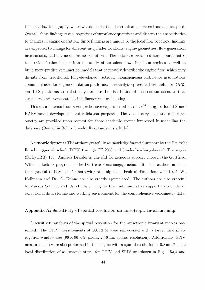
the local flow topography, which was dependent on the crank-angle imaged and engine speed.
Overall, these findings reveal requisites of turbulence quantities and discern their sensitivities
to changes in engine operation. Since findings are unique to the local flow topology, findings
are expected to change for different in-cylinder locations, engine geometries, flow generation
mechanisms, and engine operating conditions. The database presented here is anticipated
to provide further insight into the study of turbulent flows in piston engines as well as
build more-predictive numerical models that accurately describe the engine flow, which may
deviate from traditional, fully-developed, isotropic, homogeneous turbulence assumptions
commonly used for engine simulation platforms. The analyses presented are useful for RANS
and LES platforms to statistically evaluate the distribution of coherent turbulent vortical
structures and investigate their influence on local mixing.
This data extends from a comprehensive experimental database28 designed for LES and
RANS model development and validation purposes. The velocimetry data and model ge-
ometry are provided upon request for those academic groups interested in modelling the
database (Benjamin Bohm, [email protected]).
Acknowledgments The authors gratefully acknowledge financial support by the Deutsche
Forschungsgemeinschaft (DFG) through PE 2068 and Sonderforschungsbereich Transregio
(STB/TRR) 150. Andreas Dreizler is grateful for generous support through the Gottfried
Wilhelm Leibniz program of the Deutsche Forschungsgemeinschaft. The authors are fur-
ther grateful to LaVision for borrowing of equipment. Fruitful discussions with Prof. W.
Kollmann and Dr. G. Kunne are also greatly appreciated. The authors are also grateful
to Markus Schmitt and Carl-Philipp Ding for their administrative support to provide an
exceptional data storage and working environment for the comprehensive velocimetry data.
Appendix A: Sensitivity of spatial resolution on anisotropic invariant map
A sensitivity analysis of the spatial resolution for the anisotropic invariant map is pre-
sented. The TPIV measurements at 800RPM were reprocessed with a larger final inter-
rogation window size (96 × 96 × 96 pixels, 2.56mm spatial resolution). Additionally, SPIV
measurements were also performed in this engine with a spatial resolution of 0.8mm28. The
local distribution of anisotropic states for TPIV and SPIV are shown in Fig. 15a,b and
44

(a) (b)
(c) (d)
axisym. contraction 3-D isotropy axisym. expansion unde!ned state
FIG. 15. Spatial distribution of the state of anisotropy within the symmetry plane (z = 0mm).
TPIV (2.56mm resolution) shown in (a) 270 bTDC and (b) 90 bTDC, while SPIV (0.8mm res-
olution) shown in (c) 270 bTDC and (d) 90 bTDC. Results shown at 800RPM and distribution
is based on 300 cycles. Streamlines from ensemble-averaged velocity fields are overlaid onto each
image.
c,d, respectively. Despite differences in the upper-left region (i.e. decrease in axisymmet-
ric contraction and increase in 3D isotropy), the majority of findings are consistent and in
agreement with findings presented in Fig. 10. Overall it can be stated that the majority
of features discussed in Sec. VI are independent of spatial resolution for the given range
(0.8mm to 2.56mm) within the FOV. This suggests that the TPIV resolution is reasonable
for the application of this study, but the measurements could be improved with a larger
spatial dynamic range.
Appendix B: Description of Box-Counting Algorithm (BCA)
For a statistical evaluation of 3D structures within TPIV measurements a Box-Counting
Algorithm (BCA) was developed to identify and characterize geometrical structures by the
number and orientation of voxels within them. In principle this methodology was outlined by
Moisy and Jimenez77. Figure 16 shows a description of the BCA based on two 2-dimensional
45

(b) step 2: apply threshold to criterion
(c) step 3: count substructures (d) step 4: merge substructure to structures
(e) step 5: cut o! undersized structures
(f) step 6: approximate shape from ellipsoid-"t
voxel
voxel belonging to structure
shape of real structure
"tted ellipsoid
criterion value
criterion value > threshold
number of substructuresbelonging to a structure
(a) step 1: apply criterion for vortical structure
Legend
FIG. 16. Pictorial description of the Box-Counting Algorithm (BCA) utilized to identify and
subsequently classify shape of individual vortical structures.
Non-complex(volume ratio V / V small)
Complex(volume ratio V / V large)e s e s
real structrue volume dierence (V / V ) tted ellipsoidLegend: e s
FIG. 17. Description of complex and non-complex structures identified with the volume ratio
Ve/Vs.
structures for simplicity.
In this work, the Q-criterion is used to identify individual vortical structures (Fig. 16a).
In principle, the BCA analysis can be performed for other flow structure analyses (e.g.
enstrophy or Lambda-Chi74). Individual grid points that exceed a threshold value (e.g.
Qnorm > 750) are identified (Fig. 16b). In a third step (Fig. 16c), substructures are
identified by all boxes satisfying the threshold in the vertical direction (i.e. columns of a third
order tensor representing the 3D volume). Neighboring boxes also satisfying the threshold
are considered to be part of this substructure. This overlap enables a stepwise merging of
substructures by forming intersecting sets based on the point sets of substructures in step 4
(Fig. 16d). Structures containing 10 points or less in total are neglected for further analysis
following Worth78 (Fig. 16e). Finally an ellipsoid is fitted to each individual structure in
space (Fig. 16f ) such that three characteristic lengths (c3 ≥ c2 ≥ c1) are defined.
The volume of an individual structure is described by the sum of all voxels belonging to
46
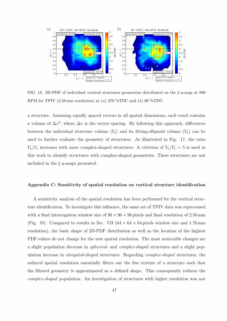
90° bTDC, 800 RPM, 96x96x96270° bTDC, 800 RPM, 96x96x96(a) (b)
2D-P
DF
2D-P
DF
0 0.2 0.4 0.6 0.8 10
0.1
0.2
0.3
0.4
0.5
0.6
0.7
0.8
0.9
1
ξ (− )
η(−
)
population: 13.9 %
neglected complex-shaped structures: 2.7 %
0
0.5
1
1.5
2
2.5
3
3.5
4
4.5
5
0 0.2 0.4 0.6 0.8 10
0.1
0.2
0.3
0.4
0.5
0.6
0.7
0.8
0.9
1
neglected complex−shaped structures: 4.5 %
0
0.5
1
1.5
2
2.5
3
3.5
4
4.5
5population: 6.3 %
26.6 %
population: 17.0 % population: 17.9 %population: 5.9 %
population: 12.9 %
ξ (− )
η(−
)
neglected complex-shaped structures: 1.7 %
26.8 %
FIG. 18. 2D-PDF of individual vortical structures geometries distributed on the ξ-η-map at 800
RPM for TPIV (2.56mm resolution) at (a) 270 bTDC and (b) 90 bTDC.
a structure. Assuming equally spaced vectors in all spatial dimensions, each voxel contains
a volume of ∆x3, where ∆x is the vector spacing. By following this approach, differences
between the individual structure volume (Vs) and its fitting-ellipsoid volume (Ve) can be
used to further evaluate the geometry of structures. As illustrated in Fig. 17, the ratio
Ve/Vs increases with more complex-shaped structures. A criterion of Ve/Vs = 5 is used in
this work to identify structures with complex-shaped geometries. These structures are not
included in the ξ-η-maps presented.
Appendix C: Sensitivity of spatial resolution on vortical structure identification
A sensitivity analysis of the spatial resolution has been performed for the vortical struc-
ture identification. To investigate this influence, the same set of TPIV data was reprocessed
with a final interrogation window size of 96× 96× 96 pixels and final resolution of 2.56mm
(Fig. 18). Compared to results in Sec. VII (64 × 64 × 64 pixels window size and 1.76mm
resolution), the basic shape of 2D-PDF distribution as well as the location of the highest
PDF-values do not change for the new spatial resolution. The most noticeable changes are
a slight population decrease in spherical- and complex-shaped structures and a slight pop-
ulation increase in elongated-shaped structures. Regarding complex-shaped structures, the
reduced spatial resolution essentially filters out the fine texture of a structure such that
the filtered geometry is approximated as a defined shape. This consequently reduces the
complex-shaped population. An investigation of structures with higher resolution was not
47

(a) (b)
(f)
(c) (d) (e)
(g) (h) (i) (j)
FIG. 19. Spatially distributed normalized frequency of occurrence (f iocc) for vortical structures with
given shape i for 800RPM 270 bTDC (top) and 90 bTDC (bottom). Results (300 cycle statistic)
are shown for reprocessed TPIV images with coarser spatial resolution of 2.56mm. Findings reveal
that the local distribution of geometrically shaped vortical structures is dependent on spatial
resolution.
possible due to low SNR values for the vortex identification criterion.
Figure 19 shows the spatially distributed f iocc of vortical structures with given geometry
for the coarser spatial resolution. Overall, the f iocc distributions are less densely populated
for the coarser resolution than the original resolution (Fig. 14). At 270 bTDC, the f iocc
distributions remain within the upper-half of the FOV and regions of higher occurrence
remain consistent for the two resolutions of interest. The only exception is for spherically-
shaped structures, which show fewer occurrences in the upper right portion of the FOV. At
90 bTDC, the distributions for f iocc < 0.25 are far sparser for the coarser resolution. With
the exception to elongated-shaped structures, distributions with f iocc > 0.25 are located in
the periphery of the mean tumble center, which is consistent with findings in Fig. 14.
The elongated-shaped distribution shows a higher population of f iocc > 0.25 for the coarser
grid. Differences in the f iocc distributions at the two resolutions of interest reveal that spatial
resolution can be a sensitive parameter for such analyses. Although only slight differences are
observed here, larger differences can be expected for larger differences in spatial resolution.
48

REFERENCES
1C. Arcoumanis and J. H. Whitelaw, “Fluid mechanics of internal combustion engines: a
review,” Proc. I. Mech. E 201C, 54–74 (1987).
2J. B. Heywood, Internal combustion engine fundamentals (McGraw-Hill, 1988).
3J. L. Lumley, Engines: an introduction (Cambridge University Press, 1999).
4J. Boree and P. Miles, “In-cylinder flow,” in Encyclopedia of automotive engineering, edited
by D. Crolla, D. E. Foster, T. Kobayashi, and N. Vaughan (Wiley, 2014) pp. 1–31.
5B. Peterson, E. Baum, B. Bohm, V. Sick, and A. Dreizler, “Spray-induced temperature
stratification dynamics in a gasoline direct-injection engine,” Proc. Combust. Inst. 35,
2923–2931 (2015).
6P. G. Hill and D. Zhang, “The effects of swirl and tumble on combustion in spark-ignition
engines,” Prog. Energy Combust. Sci. 20, 373–429 (1994).
7J. L. Lumley, “Early work on fluid mechanics in the ic engine,” Ann. Rev. Fluid Mech.
33, 319–338 (2001).
8B. Peterson, E. Baum, B. Bohm, V. Sick, and A. Dreizler, “High-speed piv and lif imaging
of temperature stratification in an internal combustion engine,” Proc. Combust. Inst. 34,
3653–3660 (2013).
9B. Peterson, E. Baum, B. Bohm, V. Sick, and A. Dreizler, “Evaluation of toluene lif
thermometry detection strategies applied in an internal combustion engine,” Appl. Phys.
B 117, 151–175 (2014).
10C. Disch, H. Kubach, U. Spicher, J. Pfeil, F. Altenschmidt, and U. Schaupp, “Investi-
gations of spray-induced vortex structures during multiple injections of a disi engine in
stratified operation using high-speed-piv,” SAE Technical Paper 2013-01-0563 (2013).
11R. Stiehl, J. Schorr, C. Kruger, A. Dreizler, and B. Bohm, “In-cylinder flow and fuel spray
interactions in a stratified spray-guided gasoline engine investigated by high-speed laser
imaging techniques,” Exp. Fluids 49, 937–947 (2010).
12M. Zhang, M. Xu, and D. L. S. Hung, “Simultaneous two-phase flow measurement of spray
mixing process by means of high-speed two-color piv,” Meas. Sci. Technol. 25, 095204
(2014).
13B. Peterson, D. L. Reuss, and V. Sick, “On the ignition and flame development in a spray-
guided direct-injection spark-ignition engine,” Combust. Flame 161, 240–255 (2014).
49

14W. Zeng, M. Sjoberg, and D. L. Reuss, “Combined effects of flow/spray interactions
and egr on combustion variability for a stratified disi engine,” Proc. Combust. Inst. 35,
2907–2914 (2015).
15T. D. Fansler, D. L. Reuss, V. Sick, and R. Dahms, “Combustion instability in spray-
guided stratified-charge engines: a review,” Int. J. Engine. Res. 16, 260–305 (2015).
16R. Dahms, T. D. Fansler, M. C. Drake, T. W. Kuo, A. M. Lippert, and N. Peters,
“Modeling ignition phenomena in spray-guided spark-ignition engines,” Proc. Combust.
Inst. 32, 3743–2750 (2009).
17B. Peterson and V. Sick, “High-speed flow and fuel imaging study of available spark energy
in a spray-guided direct-injection engine and implications on misfires,” Int. J. Engine Res.
11, 313–329 (2010).
18D. Bradley, M. Lawes, and C. G. W. Sheppard, “Combustion and the thermodynamic
performance of spark ignition engines,” I. Mech. E. 214, 257–268 (2000).
19C. Mounaım-Rousselle, L. Landry, F. Halter, and F. Foucher, “Experimental characteris-
tics of turbulent premixed flame in a boosted spark-ignition engine,” Proc. Combust. Inst.
34, 2941–2949 (2013).
20B. Peterson, E. Baum, B. Bohm, and A. Dreizler, “Early flame propagation in a spark-
ignition engine measured with quasi 4d-diagnostics,” Proc. Combust. Inst. 35, 3829–3837
(2015).
21P. Abraham, K. Liu, D. Haworth, D. Reuss, and V. Sick, “Evaluating large-eddy simu-
lation (les) and high-speed particle image velocimetry (piv) with phase-invariant proper
orthogonal domcomposition (pod),” Oil Gas Sci. and Technol. 69, 41–59 (2014).
22B. Peterson, D. L. Reuss, and V. Sick, “High-speed imaging analysis of misfires in a
spray-guided direct injection engine,” Proc. Combust. Inst. 33, 3089–3096 (2011).
23R. Stiehl, J. Bode, J. Schorr, C. Kruger, A. Dreizler, and B. Bohm, “Influence of
intake geometry variations on in-cylinder flow and flow-spray interactions in a strati-
fied disi engine captured by time-resolved piv,” Int. J. Engine Res. online first, doi:
10.1177/1468087416633541 (2016).
24D. C. Haworth, “Large-eddy simulation of in-cylinder flows,” Oil Gas Sci. Technol. Review
IFP 54, 175–185 (1999).
25I. Celik, I. Yavuz, and A. Smirnov, “Large eddy simulations of in-cylinder turbulence for
internal combustion engines: a review,” Int. J. Engine Res. 2, 119–148 (2001).
50
26M. C. Drake and D. C. Haworth, “Advanced gasoline engine development using optical
diagnostics and numerical modeling,” Proc. Combust. Inst. 31, 99–124 (2009).
27M. Baumann, F. diMare, and J. Janicka, “On the validation of les applied to internal
combustion engine flows - part ii: numerical analysis,” Flow Turb. Combust. 92, 299–317
(2014).
28E. Baum, B. Peterson, B. Bohm, and A. Dreizler, “On the validation of les applied to
internal combustion engine flows - part i: comprehensive experimental database,” Flow
Turb. Combust. 92, 269–297 (2014).
29C. Lacour and C. Pera, “An experimental database dedicated for the study and modeling of
cyclic variability in spark-ignition engines with les,” SAE Technical Paper 2011-01-1282
(2011).
30T. D. Fansler, “Turbulence production and relaxation in bowl-in-piston engines,” SAE
Technical Paper 930479 (1993).
31D. L. Reuss, “Cyclic variability of large-scale turbulent structures in directed and undi-
rected ic engine flows,” SAE Technical Paper 2000-01-0246 (2000).
32X. Baby, A. Duponts, A. Ahmed, W. Deslandes, G. Charnay, and M. Michard, “A
new methodology to analyze cycle-to-cycle aerodynamic variations,” SAE Technical Paper
2002-01-2837 (2002).
33M. Voisine, L. Thomas, J. Boree, and P. Rey, “Spatio-temporal structure and cycle to
cycle variations of an in-cylinder tumbling flow,” Exp. Fluids 50, 1393–1407 (2011).
34Y. Cao, E. Kaiser, J. Boree, B. Noack, L. Thomas, and S. Guilain, “Cluster-based analysis
of cycle-to-cycle variations: application to internal combustion engines,” Exp. Fluids 55,
1837 (2014).
35V. Sick, M. C. Drake, and T. D. Fansler, “High-speed imaging for direct-injection gasoline
engine research and development,” Exp. Fluids 49, 937–947 (2010).
36V. Chan, D. Bamhart, C. Garner, N. Halliwell, and J. Coupland, “A unified system
for holographic measurement in fluid and solid mechanics: application of the system to
volumetric flow measurement in an i.c. engine,” in In: Part of the SPIE Converence on
Optical Diagnositcs for Fluids/Heat/Combustion and Photomechanics for Solids, Vol. 3783
(1999) pp. 110–117.
37P. O. Calendini, T. Durverger, A. Lecerf, and M. Trinite, “In-cylinder velocity measure-
ments with stereoscopic particle image velocimetry in a si engine,” SAE Technical Paper
51

2000-01-1798 (2000).
38J. Coupland, C. Garner, R. Alcock, and N. Halliwell, “Holographic particle image ve-
locimetry and its application in engine development,” Journal of Physics: Coference Series
45, 29–37 (2006).
39I. Bucker, D. Karhoff, M. Klass, and W. Schroder, “Stereoscopic multi-planar piv mea-
surements of in-cylinder tumbling flow,” Exp. Fluids 53, 1993–2009 (2012).
40E. Baum, B. Peterson, C. Surmann, D. Michaelis, B. Bohm, and A. Dreizler, “Investigation
of the 3d flow field in an ic engine using tomographic piv,” Proc. Combust. Inst. 34, 2901–
2910 (2013).
41T. VanOverbruggen, M. Klaas, B. Bahl, and W. Schroder, “Tomographic particle-image
velocimetry analysis of in-cylinder flows,” SAE International Journal of Engines 8(3),
1447–1461 (2015).
42S. B. Pope, Turbulent flows (Cambridge University Press, 2000).
43D. Freudenhammer, E. Baum, B. Peterson, B. Bohm, B. Jung, and S. Grundmann, “Vol-
umetric intake flow measurements of an ic engine using magnetic resonance velocimetry,”
Exp. Fluids 55, 1724 (2014).
44D. Freudenhammer, B. Peterson, C.-P. Ding, B. Bohm, and S. Grundmann, “The influence
of cylinder head geometry variations on the volumetric intake flow captured by magnetic
image velocimetry,” SAE Int. J. Engines 8(4), 1826–1836 (2015).
45B. Wieneke, “Volume self-calibration for 3d particle image velocimetry,” Exp. Fluids 45,
549–556 (2008).
46G. T. Herman and A. Lent, “Iterative reconstruction algorithms,” Computers in Biology
and Medicine 6, 273–294 (1976).
47R. Adrian, “Dynamic ranges of velocity and spatial resolution of particle image velocime-
try,” Meas. Sci. Technol. 8, 1393–1398 (1997).
48R. Keane and R. Adrian, “Optimization of particle image velocimeters. part 1: double
pulsed systems,” Meas. Sci. Technol. 1, 1202–1215 (1990).
49J. Luff, T. Drouillard, A. Rompage, M. Linne, and J. Hertzberg, “Experimental uncer-
tainties associated with particle image velocimetry (piv) based velocity algorithms,” Exp.
Fluids 26, 36–54 (1999).
50M. Megerle, V. Sick, and D. Reuss, “Measurement of digital particle image velocimetry
precision using electro-optically created particle-image displacements,” Meas. Sci. Technol.
52
13, 997–1005 (2002).
51D. L. Reuss, M. Megerle, and V. Sick, “Particle-image velocimetry measurement errors
when imaging through a transparent engine cylinder,” Meas. Sci. Technol. 13, 1029–1035
(2002).
52J. Westerweel, “Fundamentals of digital particle image velocimetry,” Meas. Sci. Technol.
8, 1379–1392 (1997).
53A. Melling, “Tracer particles and seeding for particle image velocimetry,” Meas. Sci. Tech-
nol. 8, 1406–1416 (1997).
54E. Baum, Laserbasierte Untersuchung innermotorischer Prozesse, PhD dissertation, Tech-
nische Universitat Darmstadt, Fachgebiet Reaktiv Stomungen und Messtechnik (RSM),
Department of Mechanical Engineering (2014).
55T. D. Fansler and D. T. French, “Cycle-resolved laser-velocimetry measurements in a
reentrant-bowl-piston engine,” SAE Technical Paper 880377 (1988).
56J. Mi, G. Nathan, and R. Luxton, “Mixing characteristics of a flapping jet from a self-
exciting nozzle,” Flow Turb. Combust. 67, 1–23 (2001).
57F. Gifford, “Statistical properties of a plume dispersion model,” Adv. Geophys. 6, 117–138
(1959).
58A. Kerstein, “Flapping model of scalar mixing in turbulence,” Phys. Fluids A. 3(12),
2838–2840 (1991).
59C. Fajardo and V. Sick, “Development of a high-speed uv particle image velocimetry
technique and application for measurements in internal combustion engines,” Exp. Fluid
46, 43–53 (2009).
60D. P. Towers and C. E. Towers, “Cyclic variability measurements of in-cylinder engine flows
using high-speed particle image velocimetry,” Meas. Sci. Technol. 15, 1917–1925 (2004).
61J. B. Ghandhi, R. E. Herold, J. S. Shakal, and T. E. Strand, “Time-resolved particle
image velocimetry measurements in an internal combustion engine,” SAE Technical Paper
2005-01-3868 (2005).
62S. Jarvis, T. Justham, A. Clarke, C. P. Garner, G. K. Hargrave, and D. Richardson,
“Motored si ic engine in-cylinder flow field measurement using time resolved digital piv
for characterization of cyclic variation,” SAE Technical Paper 2006-01-1044 (2006).
63M. Fogelman, J. Lumley, D. Rempfer, and D. Haworth, “Application of the proper or-
thogonal decomposition to datasets of internal combustion engine flows,” J. Turbul. 5(23),
53

1–18 (2004).
64H. Chen, D. L. Reuss, D. L. S. Hung, and V. Sick, “A practical guide for using proper
orthogonal decomposition in engine research,” Int. J. Engine Res. 14, 307–319 (2012).
65H. Chen, D. L. Reuss, and V. Sick, “On the use and interpretation of proper orthogonal
decomposition of in-cylinder engine flows,” Meas. Sci. Technol. 23, 085302 (2012).
66B. Bohm, C. Heeger, I. Boxx, W. Meier, and A. Dreizler, “Time-resolved conditional flow
field statistics in extinguishing turbulent opposed jet flames using simultaneous high speed
piv/oh-plif,” Proc. Combust. Inst. 32, 1647–1654 (2009).
67J. Dannemann, K. Pielhop, M. Klaas, and W. Schroder, “Cycle resolved multi-planar
measurements in a four-valve combustion engine,” Exp. Fluids 50, 961–976 (2011).
68P. C. Miles, “In-cylinder turbulent flow structure in direct-injection, swirl-supported diesel
engines,” in Flow and combustion in reciprocating engines, edited by C. Arcoumanis and
T. Kamimoto (Springer, 2014) pp. 173–256.
69L. Graftieaux, M. Michard, and N. Grosjean, “Combining piv, pod, and vortex identifi-
cation algorithms for the study of unsteady turbulent swirling flows,” Meas. Sci. Technol.
12, 1422 (2001).
70K. S. Choi and J. L. Lumley, “The return to isotropy of homogeneous turbulence,” J. Fluid
Mech. 436, 59–84 (2001).
71P. C. Miles, B. H. RempelEwert, and R. D. Reitz, “Experimental assessment of a nonlinear
turbulent stress relation in a complex reciprocating engine flow,” Exp. Fluids 47, 451–461
(2009).
72M.M. Rogers and P. J. Moin, “The structure of the vorticity field in homogeneous turbulent
flows,” J. Fluid Mech. 176, 33–66 (1987).
73J. Jeong and F. Hussain, “On the identification of a vortex,” J. Fluid Mech.. 285, 69–94
(1995).
74P. Chakraborty, S. Balachandar, and R. J. Adrian, “On the relationships between local
vortex identification schemes,” J. Fluid Mech. 535, 189–214 (2005).
75C. R. Hunt, A. A. Wray, and P. Moin, “Eddies, stream, and the convergence zones in
turbulent flows,” Center for Turbulence Research Report CTR-S88 (1994).
76C. Wolf and R. Hornschemeyer, “Tomographic piv measurements in the shear layer of a
bluff-body wake flow,” AIAA Paper 2011-3084 (2011).
77F. Moisy and J. Jimenez, “Geometry and clustering of intense structures in isotropic
54

turbulence,” J. Fluid Mech. 513, 111–133 (2004).
78N. Worth, Tomographic-PIV measurement of coherent dissipation scale structures, PhD
dissertation, University of Cambridge (2010).
55