edible frog harvesting in indonesia: evaluating its …eprints.jcu.edu.au/1118/2/02whole.pdf ·...
TRANSCRIPT
EDIBLE FROG HARVESTING IN INDONESIA:
EVALUATING ITS IMPACT AND ECOLOGICAL CONTEXT
Thesis submitted by
Mirza Dikari KUSRINI BSc (IPB) MSc (IPB)
In February 2005
for the degree of Doctor of Philosophy
in Zoology and Tropical Ecology
within the School of Tropical Biology
James Cook University

ELECTRONIC COPY
I, the undersigned, the author of this work, declare that the electronic copy of this thesis provided to the James Cook University Library, is an accurate copy of the print thesis submitted, within the limits of the technology available. _______________________________ _______________ Signature Date
iii
ABSTRACT
Frogs are harvested in Indonesia for both domestic consumption and export.
Concerns have been expressed about the extent of this harvest, but there have been no
detailed studies on the edible frog trade in Indonesia, or on the status or population
dynamics of the harvested species. To investigate the possible impact of this practise, I
collected data on harvesting and trading of frog legs in Java, Indonesia. I also
investigated the ecology and population dynamics of the three species that are most
heavily harvested: Fejervarya limnocharis-iskandari complex, F. cancrivora and
Limnonectes macrodon.
The first step of the study quantified the extent of the Indonesian edible frog leg
trade for export and domestic purposes. Harvesting is an unskilled job and serves as
livelihood for many people. There is no regulation of this harvest, and species taken and
size limits are governed by market demand. The most harvested species in Java are F.
cancrivora and L. macrodon. Harvests occur all year long. The number of frogs
harvested fluctuates and is controlled by natural forces such as dry/wet seasons, moon
phase, and planting seasons. Records of the international trade in Indonesian frog legs
are available from 1969 to 2002; the mass of frozen frog legs exported has increased
over the years. I used data on the relative weights of frogs and their legs to estimate how
many frogs were represented by the export records. In 1999-2002 an average of
3,830,601 kg of frozen frog legs were exported annually; this represents an export
harvest of approximately 28 to 142 million frogs, all with masses greater than 80 g, the
minimum size of animals that have legs considered suitable for export. I used data
collected by following frog hunters in the field to assess their capture rates and the
numbers and sizes of frogs captured. I found that only about one-eighth of frogs
iv
captured are of sizes acceptable for export, and therefore estimate that the domestic
market is approximately 7 times as large as the export market.
In the second step of the study, I used field data on F. limnocharis-iskandari
complex, F. cancrivora and L. macrodon to gain greater understanding of the
population biology and dynamics of the harvested species. Populations of F.
limnocharis-iskandari complex and F. cancrivora were studied in six rice fields in West
Java during the planting seasons of 2002 and 2003. Both F. limnocharis-iskandari
complex and F. cancrivora were abundant in the rice fields, with estimated overall
mean densities of 193.71 and 39.76 per hectare. The mean density of F. cancrivora was
very similar to that of unharvested populations in Malaysia (8.6 – 91.2 per hectare)
(Jaafar, 1994) and was much higher than the mean density (0.7 frogs/ha) found for Rana
tigerina, the larger species of edible Indian paddy field frog investigated by Dash and
Mahanta (1993). These comparisons suggest that densities of F. cancrivora in Javan
rice fields are relatively high, despite ongoing harvesting pressure. F. limnocharis-
iskandari complex and F. cancrivora were able to breed continuously all year without
an apparent season. Both species showed sexual size dimorphism, with females larger
than males. Both appear to be short lived.
The population dynamics of L. macrocodon were observed at two stream sites
West Java: Cilember and Ciapus Leutik. The habitat at Ciapus Leutik is relatively
heavily modified bu human activity, while Cilember is in a nature reserve and ls less
disturbed. A mark recapture study was conducted once a month between June 2002 and
May 2003 (a continuous 12 month sampling period), and in January, April and July
2004. Skeletochronological analysis of phalanges removed during toe clipping suggests
that this species lives longer than F. cancrivora or F. limnocharis-iskandari complex.
Recapture rates of L. macrodon in both locations were low and more frogs were
v
observed during periods of higher rainfall. In this study, more L. macrodon were found
at Cilember than at Ciapus Leutik stream. It is unclear whether the low number of frogs
at Ciapus Leutik was caused by over-harvesting or by other factors. There is a need for
further monitoring to obtain a greater understanding of the population dynamics of this
species.
In conjunction with my field work, I measured a number of parameters to
determine the type and extent of pesticide residues present in rice fields, and to attempt
to determine whether those and another potential stressor, drought, might be affecting
the morphology, body condition, or developmental stability of frogs. I also surveyed
populations of the rice field frogs and L. macrodon for the emerging disease
chytridiomycosis, which could strongly affect the population dynamics of the frogs.
Two types of pesticide residues were detected in water and soil: organochlorine
(lindane, aldrin, heptachlor, dieldrin and endosulfan) and organophospate (chlorpyrifos
and diazinon). Six organochlorines type (BHC, lindane, aldrin, heptachlor, dieldrin and
endosulfan) and three organophosphates (propenofos, chlorpyrifos and diazinon) were
detected in the livers and leg muscles of both frog species. Almost all pesticide residues
were low compared to the Maximum Residue Limit set by WHO and the Government
of Indonesia although a few individuals showed higher pesticide residues contents.
Pesticide residue levels did not appear to be related to any measure of frog condition or
stress. Both species of rice field frogs exhibited relatively low percentages of
abnormalities, probably within the normal range. Only F. limnocharis-iskandari
complex consistently exhibited levels of fluctuating asymmetry in excess of
measurement error. Levels of asymmetry differed between characters. Higher limb
asymmetries were elevated in 2002 compared to 2003, whilst body condition was lower
in 2003. It is possible that the lower body condition in 2003 was caused by stress from
vi
an environmental factor, in this case the drought in that year. It is clear that for both F.
limnocharis-iskandari complex and F. cancrivora, fluctuating asymmetry is not a
powerful indicator of stress. There was no sign of chytrid infection in any samples of
the three species.
To assess the impact of harvesting, I used two approaches. I developed a model
of the population dynamics of F. cancrivora and ran simulations for ranges of
parameters including harvesting rate. The simulation indicated that current levels of
harvest may be near the maximum level sustainable by the population. My second
approach was to compare data on the population biology and distribution of both
Fejervarya species to criteria for assessing the conservation status of the species, i.e.
IUCN Red Categories and the CITES Res. Conf. 9.24 on the Criteria for Amendment of
Appendices I and II.
My assessment using listing criteria showed that neither F. limnocharis-
iskandari complex or F. cancrivora are qualified for inclusion into any IUCN Red List
and CITES Appendices. On the other hand, more consideration needs to be given to L.
macrodon. This frog is not qualified for inclusion in CITES Appendix I. At present, it
is not possible to determine whether this species could be listed as vulnerable or in
CITES Appendix II due to a lack of data, such as survivorship among stages, and
habitat size, on the population biology of this species.
Recommendations for management of the harvest include: 1) regular monitoring
of this trade especially in other islands such as Sumatra by the scientific authority of
CITES (The Indonesian Institute of Science or Lembaga Ilmu Pengetahuan Indonesia,
LIPI), 2) regular monitoring of the numbers of export companies and their middleman,
3) developing a simple identification key and distributing it to the middlemen to ensure
correct identifications, 4) assessing the possibility of breeding local frogs for this trade

vii
to replace the farming of the exotic frog Rana catesbeiana, and 5) ensuring that harvest
is limited to species that are not adversely impacted.
viii
ACKNOWLEDGMENTS
I thank Allah, God the Almighty that has guided me throughout my life, including
this part of my life journey as student. More than 30 years ago as a toddler I stood
watching buckets of frogs captured the night before from the neighbouring rice fields by
my father and brother. Little did I know at that time that this personal fascination would
result in this dissertation.
The project was made possible by various funding. The Australian Development
Scholarship gave a scholarship for the author as part of a scholarship program for
Indonesian Government Employees. Funding, mostly from the Wildlife Conservation
Society, with additional funding from Indonesian Reptile Amphibian Trader Association,
Research Office Institut Pertanian Bogor and James Cook University, made fieldwork
possible. I thank all the funding agencies for their help.
Many people have supported my study, emotionally and scientifically. Without
them, I doubt if I could have manage to finish my study on time, and for that I wish to
give them all my sincerest thanks.
In Australia, I am grateful for the advice and assistance from my supervisor
Assoc. Prof. Ross A. Alford, who has not only supported my research but also gave me
valuable advice and comments on various matters. He has also inspired me to do more
frog research in the future, so thank you very much Ross. I could not find better
supervisor than you.
I also wish to thank my fellow students, some of them are now alumni’s, Adam
Felton, Kay Bradfield, Doug Woodhams, Jodi Rowley, Nicole Kenyon and Kim

ix
Hauselberger and research assistants (Tracy Langkilde, Anthony Backer, Sara Townsend
and Carryn Manicom) in the frog lab, who has shared the same passion for frog research
while trying to maintain humour during the gruelling days as uni-fellows. I thank them
for the companionship and insight on various matters. Jodi Rowley has opened her heart
and her home during my last 2 weeks in Townsville. For this I thank her – your book
collections also helped me a lot! Adam Felton and Richard Retallic prepared me for the
rigours of skeletochronology analysis in tropical frogs, while Sara Townsend, Sue Reilly
from the histological lab, and Kim Hauselberger helped me during my histology work.
Kay Bradfield practically showed me step-by-step analysis for developmental stability
analysis. I also want to thank my ALO during my study: Janelle Walsh and Alex
Salvador. They both ensured that my transition as a student went smoothly. Special
thanks for my editor; Tim Harvey who edited the grammatical works in this thesis.
I also wish to thank my fellow Indonesian friends and family for the
companionship and joyful sharing of our country during my time in Townsville. A
special thanks is given to Yeni Mulyani – who was in Darwin - who has been a great
listener to my woes and joys even though she was practically in the same boat as I.
In Indonesia, my greatest thanks and appreciation is for Dr. Ani Mardiastuti and
family. Not only has she encouraged me to further my study but also has fully supported
my research by giving advice and also acting as host during my stay in Bogor. I thank her
family (pak Agus Pakpahan, Angga, Andya and Mbah Mandi) for their hospitality. I am
also deeply grateful for the help of my assistant Anisa Fitri, SHut. For more than three
years Fitri had been invaluable in assisting me with her great administration skills and
practicality. With great determination she managed all the dirty work of contacting
x
farmers, harvesters, traders and managing volunteers while ensuring that data taken met
the requirement of her boss. Tackling this research would have been impossible without
the help of volunteers, so I would like to thank Hijrah Utama (Aji), Mommad Dede Nasir
(Dogen), Sumantri Radiansyah (Abenk), Ita Novita Sari, Vivien Lestari, Ian Budarto,
Sudrajat, Reddy Rahmadi, Dadi Ardiansyah, Edi Sutrisno and many more who gave their
time to help me. In 2001, Yoshiko Hikariati accompanied me sorting export data from the
crumbling old books in the Statistical Office (BPS) in Pasar Baru, for this I thank you.
I would also like to thank Dr. Djoko T. Iskandar (ITB), Dr. Tonny Soehartono
(CI-IP), Ibu Mumpuni (Museum Zoologicum Bogoriense), Bapak George Saputra
(IRATA), Bapak Frank B. Yuwono and Dr. Damayanti Buchari (WT-IP) who gave me
advice before and during this research, and Dr. Asep Nugraha, MS from Agribio in
Bogor who assisted me with the pesticide work. Dr. Ibrahim Jaafar from Malaysia has
kindly sent me a copy of his thesis and for this I thank him. I thank Jurusan Konservasi
Sumberdaya Hutan (JKSH), Fakultas Kehutanan IPB for cooperation during my stay in
Bogor. I also thank my colleagues in JKSH, especially Dr. Lilik B. Prasetjo and his lab
who helped me with the mapping, and Arzyana Sunkar, MSc who not only joyfully
volunteered in the field but also reminded me how to operate Powersim. I would also
thank the farmers who have given me access to their rice fields, especially to Kang Ade
(Subang), Kang Karmo (Karawang) and the people of Ciptarasa (Sukabumi). Special
thanks are also given to the harvesters and traders especially Wanto in Bogor, who has
given me an insight into their world.
Last but not least, I thank my family for their support during my study. My
Mother, Zaghleila Azizah has supported me – not only financially but mostly emotionally

xi
during all my years as a student (it is a long way from my kindergarten days!). I also
thank my sisters and brother (Etoy, Mia, Latifah and Ai) and the in-laws. Wanda
Wirianata assisted me during preliminary work in Ciptarasa and for this I am grateful.
My mother in law and Latifah opened their house for me to use during my stay in Jakarta
and I thank them for their hospitality.
Huge appreciation and thanks go to my husband, Ramadin Wahono Subekti, who
stopped all his work and took care of our children while I was away in the fields, busy in
lab or writing, which has practically been most of the time during our stay in Townsville.
I thank my children, Benz Satrio Utomo Ramadin and Adinda Sri Yuani Ramadin for
their understanding and support. I love you and I have been blessed. Terima kasih.

xii
TABLE OF CONTENTS
Title ……………………………………………………………………………. i
Statement of Access …………………………………………………………… ii
Abstract ………………………………………………………………………... iii
Acknowledgment ……………………………………………………………… viii
Table of Contents ……………………………………………………………… xii
List of figures ………………………………………………………………….. xvii
List of tables …………………………………………………………………… xxiii
Statement of Sources …………………………………………………………... xxvii
CHAPTER 1. GENERAL INTRODUCTION …………………………………. 1
1.1 Harvest from the wild ……………………………………………….. 1
1.2 Frogs for human use with the emphasize of Indonesian frogs and
threats to their existence ……………………………………...……..
3
1.3 The sustainability of wildlife harvest ……………………………….. 7
1.4 Research focus ……………………………………………………... 10
1.5 Research aims ……………………………………………………… 10
1.6 Thesis outline ………………………………………………………. 11
CHAPTER 2. INTERNATIONAL TRADE IN INDONESIAN FROG LEGS .. 12
2.1 Introduction …………………………………………..……………… 12
2.2 Methods …………………………………………...…………………. 13
2.2.1 Harvest estimation ………………………………………….. 13
2.2.2 Exporter profiles …………………………………………… 15
2.3 Results …………………………………………………………….… 16
2.3.1 Species exported ………………….………………………… 16
2.3.2 The volume and value of Indonesian frog leg exports ……... 17
2.3.3 Destinations of exported frog legs ………………………..... 19
2.3.4 Frog Export Profile …………………………………………. 20
2.3.5 The sources of exported frog legs ………………….…...…… 23
2.3.6 Number harvested for export ………………………...……… 24
2.4 Discussion …………………………………………………...………
25
xiii
CHAPTER 3. EDIBLE FROG HARVESTING AND THE STRUCTURE OF
THE DOMESTIC MARKET ………………………..………...
29
3.1 Introduction ………………………………………………………… 29
3.2 Methods …………………………………………………………….. 29
3.3 Results ……………………………………………………………….. 32
3.3.1 Species harvested …………..……………………………… 32
a. Species in trade …………………………………………. 32
b. Frog sizes ………………………………………………..
34
3.3.2 The process of harvesting frog and the characteristics of
harvester ……………………………………………….
34
a. Profiles of harvesters, middle men and traders ……… 34
b. Harvesting Techniques ……………………………..… 36
c. Harvesting effort ………………………………………. 37
3.3.3 Market structure ……………………………………….… 38
a. Price …………………………………………………… 40
b. Levels of income and profit …………………………… 41
c. Sustainability …………………………………………. 45
d. Number of frogs sold in local market …………………. 46
3.4. Discussion …………………………….…………………………... 48
CHAPTER 4. STUDY SPECIES AND SITES ……………………………….. 55
4.1 Introduction …………………………………………………………. 55
4.2 Description and distribution of the common edible frogs …………... 55
4.2.1 Paddy field frog, Fejervarya limnocharis ………………….. 56
4.2.2 The crab eating frog, Fejervarya cancrivora ……………… 62
4.2.3 The Giant Javanese Frog, Limnonectes macrodon ………... 65
4.3 The locations ………………………………………………………... 69
4.3.1 Rice fields …………………………………………………… 71
a. Location …………………………………………………. 71
b. Rice planting method and management …………………. 77
4.3.2 Streams …………………………………………………….
82
xiv
CHAPTER 5. POPULATION DYNAMICS OF F. LIMNOCHARIS AND F.
CANCRIVORA …………………………………………………..
85
5.1 Introduction ………………………………………………………… 85
5.2 Methods ……………………………………………………………... 87
5.2.1 Population study …………………………………………… 87
5.2.2 Determination of sex ……………………………………….. 89
5.2.3 Skeletochronology analysis ………………………………… 90
5.2.4 Sampling bias ………………………………………………. 91
5.2.5 Movement of F. cancrivora ………………………………… 91
5.3 Data analysis ……………………………………………………….. 92
5.4 Results ………………………………………………………………. 94
5.4.1 Traits of F. limnocharis and F. cancrivora ………………... 94
5.4.2 Demographic analysis ……………………………………… 100
5.4.3 Sampling effects .……….…………………………………. 113
5.4.4 Population estimates ………………………………………... 114
5.4.5 F. cancrivora movement …………………………………… 119
5.5 Discussion …………………………………………………………... 120
CHAPTER 6. THE POPULATION BIOLOGY OF LIMNONECTES
MACRODON …………………………………………………...
128
6.1 Introduction …………………………………………………………. 128
6.2 Methods ……………………………………………………………... 128
6.2.1 Location ……………………………………………………. 128
6.2.2 Sampling ……………………………………………………. 131
6.2.3 Data analysis ……………………………………………….. 133
6.3 Results ……………………………………………………………… 135
6.3.1 Microclimate ……………………………………………….. 135
6.3.2 Captures ……………………………………………………. 136
6.3.3 Traits of L. macrodon ……………………………………… 140
6.3.4 The biology of L. macrodon ……………………………….. 145
6.3.5 Population dynamic and population structure …………….. 147
6.3.6 Microhabitat use …………………………………………… 154
6.3.7 Movement …………………………………………………… 154
6.4 Discussions …………………………………………………………. 156

xv
CHAPTER 7. ENVIRONMENT STRESS …………………………………….. 161
7.1 Introduction …………………………………………………………. 161
7. 2. Methods ……………………………………………………………. 164
7.2.1. Study area ………………………………………………….. 164
7.2.2 Morphological abnormalities ……………………………… 164
7.2.3. Pesticide analysis in rice fields ……………………………. 165
a. Sample collection ……………………………………….. 165
b. Pesticide residue analysis ……………………………….. 166
c. Statistical analysis ……………………………………….. 167
7.2.4 Developmental Stability Analysis …………………………... 168
7.2.5 Chytridiomycosis …………………………………………… 170
7.3 Results …………………………………………………………….. 171
7.3.1 Morphological abnormalities ……………………………… 171
7.3.2 Pesticide levels ..…………………………………………… 177
7.3.3 Fluctuating Asymmetry ……………………………………. 189
7.3.4 Chythridiomycosis ………………………………………….. 197
7.4 Discussion …………………………………………………………... 197
CHAPTER 8. CONSERVATION STATUS OF THE EDIBLE FROGS …….. 205
8.1 Introduction …………………………………………………………. 205
8.2 Methods ……………………………………………………………... 207
8.2.1 Modelling the impact of frog harvest ………………………. 207
a. General model description ………………………………. 207
b. Harvesting simulation model ……………………………. 208
8.2.2. Conservation status ………………………………………... 211
8.3 Result ……………………………………………………………….. 213
8.3.1 Harvesting modelling ………………………………………. 213
a. The simulation …………………………………………… 213
b. Model limitation …………………………………………. 213
8.3.2 Conservation status ………………………………………… 221
8.4 Discussions ………………………………………………………….. 225
CHAPTER 9. GENERAL DISCUSSIONS AND CONCLUSION …………… 228
9.1 Introduction ………………………………………………………….. 228
9.2 The extent of the Indonesian edible frog leg trade ………………….. 228

xvi
9.3 The population status of the harvested species ……………………... 230
9.4 Environment stressor ……………………………………………….. 232
9.5 The sustainability of harvest and the conservation status of
the edible frogs ……………………………………………………...
234
9.6 Recommendations …………………………………………………... 238
REFERENCES ………………………………………………………………… 240

xvii
LIST OF FIGURES
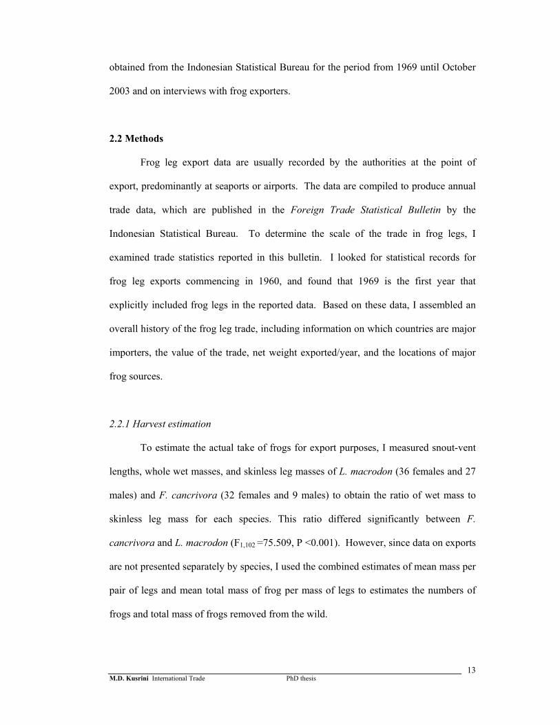
Figure 2-1. The correlation between leg mass (g) and body mass (g) of F. cancrivora and L. macrodon based on captured frogs from harvesters ……………………..……………………………………...
15
Figure 2-2. Volume of frog legs exported by Indonesia from 1969 – 2002. 3 Moving average: A sequence of averages that are computed from the every three data series to smoothes the fluctuations in data, thus showing the pattern or trend more clearly ………………………..….
18
Figure 2-3. Value of frog legs exported by Indonesia from 1969 – 2002. FOB value: value of export which still included shipping costs and the insurance costs) from the point of manufacture to a specified destination ………………………………………………….………..
18
Figure 2-4. Processing frog legs for export (top) and box of skinless frog leg ready to be shipped (centre and below) …………………...…………
22
Figure 2-5. The volume of frog legs exported out of ports in four main islands in Indonesia …………………...………………………………………..
24
Figure 2-6. Total rice field area in several main islands in Indonesia 1983 to 1999. Data taken from Indonesian Statistical Bureau ………
27
Figure 3-1. Frogs sold in the markets, either alive (centre) or as skinless legs (top). Below, a costumer buy frog legs in Madiun, East Java ……...
33
Figure 3-2. Equipment used to capture frogs include lamps, bags and bamboo pole with net in West Java (left) or three headed spears in East Java (right) …………………………………………………………….….
39
Figure 3-3. Rejected frog legs with bruised marks ……………………………...
39
Figure 3-4. The web of frog leg supply from harvesters to consumers usually consist of hunters, middle men, supplier and then the costumer itself either an export company that will distributed the legs to overseas or local consumers in the market …………………………………….....
40
Figure 3-5. Rana catesbeiana (top) and abandoned frog farm in Malang, East Java (below) …………………………………………….
47
Figure 4-1. Differences in webbing between the toes of F. limnocharis, F. cancrivora and L. macrodon ……………..…………………………
58
Figure 4-2. The distribution of F. limnocharis in Indonesia. Points were made based on specimens stored at MZB and additional survey …………
61
Figure 4-3. The distribution of F. cancrivora in Indonesia. Points are based on localities of specimens stored at MZB and additional surveys ……
63
xviii
Figure 4-4. Various type of habitat for Limnonectes macrodon: A – stream with fast flowing water and boulder in Caringin (Bogor), B – stream flowing across rice fields in Cilengkong (Sukabumi) , C - Small stream in Cilabruk (Sukabumi) with closed canopy; D – irrigation tributaries in Situ Gunung (Sukabumi) ………………………….….
67
Figure 4-5. The distribution of L. macrodon in Indonesia. Points were made based on specimens stored at MZB and additional surveys ………...
68
Figure 4-6. Monthly rainfall in Caringin and Darmaga from January 2002 to December 2003. Data from Caringin is taken from Ciawi Station, whilst data for Darmaga is from Darmaga Bogor station. Data source: Stasiun Klimatologi Darmaga Bogor, Badan Meteorologi dan Geofisika Balai Wilayah II) ……………………………….…..
72
Figure 4-7. Monthly rainfall in Karawang and Subang from January 2002 to December 2003. Data is the same for both locations, since it was only served by Cilamaya Karawang station. Data source: Stasiun Klimatologi Darmaga Bogor, Badan Meteorologi dan Geofisika Balai Wilayah II …………………………………………………….
73
Figure 4-8. Sampling sites in paddy fields in West Java ……….………………..
76
Figure 4-9. Various stages of rice fields. A and B are rice fields in Caringin during the second and sixth weeks after planting. Fallow periods in Karawang (C) and Sukabumi (D). Rice plants ready to be harvested in Subang (E) and terrace rice fields during the sowing period in Mount Halimun National Park enclave (F) …………………………
80
Figure 4-10. Sampling sites in streams …………………………………….
84
Figure 5-1. Snout vent length of F. limnochari- iskandari complex and F. cancrivora ……..
96
Figure 5-2. Body mass of F. limnocharis- iskandari complex and F. cancrivora
97
Figure 5-3. Relationship between snout vent length (mm) and mass (gram) of F. limnocharis-iskandari complex and F. cancrivora …………………
99
Figure 5-4A. Female F. limnocharis-iskandari complex (SVL = 41.5 mm, mass = 5 g), 1 LAG (arrow): scale 40 µm …………………………………
101
Figure 5-4B. Male F. limnocharis-iskandari complex, no LAGs, SVL = 43 mm, mass = 6.4 g. (MC = Marrow cavity; EB = Endosteal Bone; PM = Periosteal Bone) ……………………………………………………
101
Figure 5-4C. Female F. cancrivora (SVL = 42 mm, mass = 4.6 g); LAG (arrow) = 1 ……………………………………………..………………………
102
Figure 5-5. Relationships between number of lines of arrested growth and snout vent length for F. limnocharis-iskandari complex and F. cancrivora. Samples were taken from West Java during September 2001 .……..
103
xix
Figure 5-6. Population structure of F. limnocharis-iskandari complex in Caringin and Darmaga for 4 sampling times (2002 and 2003) based on snout vent length (mm) of individuals at first capture in a sampling episode ……………….
104
Figure 5-7. Population structure of F. limnocharis-iskandari complex in Karawang-1 and Karawang-2 for 4 sampling times (2002 and 2003) based on snout vent length (mm) of individuals at first capture in a sampling episode ………………………………………………………….…..
105
Figure 5-8. Population structure of F. limnocharis-iskandari complex in Subang-1 and Subang-2 for 4 sampling times (2002 and 2003) based on snout vent length (mm) of individuals at first capture in a sampling episode ..………………
106
Figure 5-9. Population structure of F. cancrivora in Caringin and Darmaga for 4 sampling times (2002 and 2003) based on snout vent length (mm) of individuals at first capture in a sampling episode ..………………....
107
Figure 5-10. Population structure of F. cancrivora in Karawang-1 and Karawang-2 for 4 sampling times (2002 and 2003) based on snout vent length (mm) of individuals at first capture in a sampling episode ………….
108
Figure 5-11. Population structure of F. cancrivora in Subang-1 and Subang-2 for 4 sampling times (2002 and 2003) based on snout vent length (mm) of individuals at first capture in a sampling episode …….………...
109
Figure 5-12. Mean size of F. limnocharis-iskandari complex and F. cancrivora in different stages of planting (top) and water level (bottom) ……………
111
Figure 5-13. Density of F. limnocharis-iskandari complex (top) and F. cancrivora (bottom) captured in three regions (1 = Bogor, 2 = Karawang; 3 = Subang) …………
112
Figure 5-14. Density of F. limnocharis-iskandari complex (top) and F. cancrivora (bottom) captured in various stages of planting and water level during 2002 and 2003
113
Figure 5-15. Mean rate of recapture for F. limnocharis-iskandari complex and F. cancrivora in different planting sites and water level ………………
115
Figure 6-1. The Ciapus Leutik stream (left ) and the Cilember stream (right) ….
130
Figure 6-2. Mean relative humidity (%), air and water temperature (oC) in the Cilember and the Ciapus Leutik Stream during sampling …………..
137
Figure 6-3. Proportion of L. macrodon captured in the Cilember stream ………..
138
Figure 6-4. Number of L. macrodon found in Cilember stream ………..……….
138
Figure 6-5. Proportion of L. macrodon captured in the Ciapus Leutik stream …..
139
Figure 6-6. Number of L. macrodon found in the Ciapus Leutik stream … 139
xx
Figure 6-7. Mean frogs found (observed and captured) in the Cilember and the
Ciapus Leutik streams during 4-monthly periods in the continuous period between June 2002 and May 2003 …………………………..
140
Figure 6-8. Size and body mass of L. macrodon in the Cilember and the Ciapus Leutik …………………………………………………….…………
141
Figure 6-9. Relationship between snout vent length (mm) and mass (gram) of L. macrodon …………………………………………….……………..
142
Figure 6-10. SVL and mass gain of five L. macrodon in the Cilember stream. Months 1–12 are June 2002 to May 2003 respectively. Trendlines are shown only for frogs recaptured more than 3 times ……………
144
Figure 6-11. Growth rate (mm SVL per month) as a function of snout vent length (SVL) for L. macrodon in the Cilember stream ……………………
145
Figure 6-12. Percentages of reproductive female L. macrodon harvested in Caringin (n = 49) …………………………………………..………
146
Figure 6-13. Relationship between body mass of L. macrodon female versus mass of eggs ………………………………………………………………
147
Figure 6-14. The proportion of frogs caught and time in months since first capture, in the Cilember stream ………………….………………….
148
Figure 6-15. Estimated number of L. macrodon population in the Cilember stream (mean + SE) during July 2002 to March 2003 ………………
149
Figure 6-16. Estimated number of L. macrodon population in the Cilember stream (mean + SE) in September to November 2002 and December 2002 to February 2003 …………………………………………..….
149
Figure 6-17A. Limnonectes macrodon from the Cilember stream with 5 LAGs; (SVL 77.86 m, mass = 61 g) ……………………………………..…
151
Figure 6-17B. Limnonectes macrodon from the Cilember stream with 3 LAGs; (SVL 101.74 mm, mass = 126.5 g) ………………………………....
151
Figure 6-18. Snout vent length (mm) versus number of line arrested growth (LAGs) for Limnonectes macrodon …………………………...
152
Figure 6-19. Population structure of L. macrodon in the Cilember (A) and the Ciapus Leutik (B) stream during three-monthly periods (June-August 2002; September- November 2002, December 2002-February 2003 and March-May 2003) based on the frequency of snout vent lengths category ………………………………………...
153
Figure 6-20. The position of L. macrodon along transect in the Cilember stream (top and the Ciapus Leutik stream (bottom). Month 1 – 12 is for June 2002 until May 2003. Month 13 = January 2004, month 14 = April 2004, month 15 = July 2004. No L. macrodon were found in
xxi
month 15 in the Cilember stream …………………………………...
154
Figure 6-21. The percentage of L. macrodon found in four types of microhabitat
155
Figure 6-22. Pool like area in the Ciapus Leutik Stream where L. macrodon was sometimes found ………………………………………………….…
159
Figure 7-1. Measurement of hind limb and front limb characters of F. limnocharis and F. cancrivora …………………………………….
169
Figure 7-2. Anophthalmy (no eye) in Rana chalconota found in Situ Gunung in 2003(top); Trauma – limb amputation in F. cancrivora (left, bottom) and Developmental abnormality – Amelia in F. cancrivora (right, bottom) ………………………………………………………
173
Figure 7-3. Prevalence of F. limnocharis-iskandari complex abnormalities per site and sampling occasions. Total sampling occasions: 29. Total sampling occasions with abnormalities = 25 ……………………………………………..
175
Figure 7-4. Prevalence of F.cancrivora abnormalities per site and sampling occasions. Total sampling occasions: 24. Total sampling occasions with abnormalities = 11 ……………………………………………...
176
Figure 7-5. Mean pesticide residues (ppm) in water, soil, livers and leg muscles of F. limnocharis-iskandari complex and F. cancrivora in Caringin …………………..
186
Figure 7-6. Mean pesticide residues (ppm) in water, soil, livers and leg muscles of F. limnocharis-iskandari complex and F. cancrivora in Darmaga
186
Figure 7-7. Mean pesticide residues (ppm) in water, soil, livers and leg muscles of F. limnocharis-iskandari complex and F. cancrivora in Karawang NP ……………
187
Figure 7-8. Mean pesticide residues (ppm) in water, soil, livers and leg muscles of F. limnocharis-iskandari complex and F. cancrivora in Karawang P ……………….
187
Figure 7-9. Mean pesticide residues (ppm) in water, soil, livers and leg muscles of F. limnocharis-iskandari complex and F. cancrivora in Subang NP ……………....
188
Figure 7-10. Mean pesticide residues (ppm) in water, soil, livers and leg muscles of F. limnocharis-iskandari complex and F. cancrivora in Subang P ………………....
188
Figure 7-11. Percent asymmetry of female F. limnocharis-iskandari complex during 2002 and 2003
193
Figure 7-12. Percent of asymmetry of male F. limnocharis-iskandari complex during 2002 and 2003
194
Figure 7-13. Pesticide and insecticide use (kg/ha)in rice fields in Indonesia ..….. 201
xxii
Figure 7-14. Mean annual rainfall in Caringin and Darmaga and Karawang and
Subang regions. ……………………………………………………...
202
Figure 8-1. Flowchart of frog population dynamics …………….………………
207
Figure 8-2. Diagram of systems that influence the population of frog ……….…
208
Figure 8-3. Model of population dynamic of Fejervarya cancrivora in rice field habitat using program Powersim …………………………………....
214
Figure 8-4. Tadpole population dynamics with level of harvesting 200 million, number of reproductive episodes per female = 4, with 1000 eggs per episode, and juvenile survival 0.72 ………………………………...
215
Figure 8-5. Dynamics of juveniles and mature frogs with level of harvesting = 200 million, number of reproductive episodes per female = 4, with 1000 eggs per episode, and juvenile survival 0.72 ……….
215
xxiii
LIST OF TABLES
Table 2-1. The proportion of whole body mass accounted for by leg mass in F. cancrivora and L. macrodon ………………………………………….
14
Table 2-2. Annual mean volume of frog legs exported and predicted number of frogs taken. A is for SVL between 89 – 162 mm, mean 101.43 mm and B is for SVL between 100 – 150 mm, mean 125 mm …………………
17
Table 3-1.
Number of people interviewed during 2001-2003 …………………..... 30
Table 3-2. Size and mass of frogs captured by harvesters ...……………………...
34
Table 3-3.
The average trip length and catch/effort per hour and per km of harvester ……………………………………………………………….
38
Table 3-4. Price of frogs (in Indonesian Rupiah) in Jakarta and West Java ……...
43
Table 3-5. Price of skinless frog legs in East Java (in Rupiah) unless stated as other form ……………………………………………………………..
44
Table 3-6. Comparative price of frogs sold from harvester to local consumer in Indonesian Rupiah, based on the maximum price available for each stakeholder …………………………………………………………….
45
Table 3-7. Harvester daily wages assuming that transportation is nil, food and price of frogs were constant …………………………………………..
45
Table 3-8. Percentage of frogs captured in category A (mass>80 grams), number in brackets refers to actual number ……………………………………
48
Table 3-9. Indonesian‘s edible frog species and their endangered status adapted from Schmuck (2002) …………………………………………………
51
Table 4-1. Mean size of specimens stored in Museum Zoologi Bogor basaed on
island group ……………………………………………………………
59
Table 4-2. Mean size of specimens stored in Museum Zoologi Bogor …………...
59
Table 4-3. Essential statistics of the six administrative areas of Java (BPS, 2002)
69
Table 4-4. Microclimate in the paddy fields of Bogor, Karawang and Subang. Data were recorded at 21.00 – 24.00 hours ……………………………
75
Table 4-5. Rice field sites surveyed for F. limnocharis-iskandari complex and F. cancrivora in West Java, Indonesia ………………………………….
78
Table 4-6. Streams and ponds surveyed for L. macrodon ………………………..
83
Table 5-1. The location and size of sampling area ……………………………….
88
Table 5-2. T-tests for sexual dimorphism in snout vent length ………………….. 95
Table 5-3. Traits of F. limnocharis-iskandari complex by site (2002 and 2003) 99
xxiv
Table 5-4. Traits of F. cancrivora by site (2002 and 2003) ………………………
98
Table 5-5. Densities of frogs captured inside bocks of paddy field and in the border. Numbers in brackets indicate the actual number captured ……
114
Table 5-6. Range and mean of the two recapture rates (number of recaptures/total frogs captured the day before) estimated for each combination of location and sampling period ………………………………………..
116
Table 5-7. F. limnocharis-iskandari complex population estimates based on the Schnabel method …………………………………………………….
118
Table 5-8. F. cancrivora population estimates based on the Schnabel method ………………………………………………………………………….
119
Table 5-9. Summary of capture rates and movement of F. cancrivora(+ SD) …...
120
Table 5-10. Comparison of density (frogs/ha) of F. limnocharis-iskandari complex in Java estimated in my study using mark-recapture data with estimates from Dash and Mahanta (1993) in India and Jaafar (1994) in Malaysia ……………..
125
Table 5-11. Comparison of density (frogs/ha) of F. cancrivora in Java estimated in my study using mark-recapture data with estimates from Dash and Mahanta (1993) in India and Jaafar (1994) in Malaysia ………………
125
Table 6-1. Summary descriptions of study sites ………………………………….
129
Table 6-2. Microclimates at the Cilember and Ciapus Leutik stream sites .………
135
Table 6-3. Traits of L. macrodon in the Cilember and Ciapus Leutik streams …...
142
Table 6-4. Snout vent length (mm) and mass (gram) gains of L. macrodon at Cilember during June 2002 to May 2003 ……………………………..
143
Table 6-5. Traits of L. macrodon captured by harvester in Caringin (West Java) ………………………………………………………………………….
146
Table 6-6. Summary of movement of L. macrodon at the Cilember stream ……
155
Table 7-1. Data on individual frogs analysed for pesticide residues in 6 rice fields
166
Table 7-2. Maximum Residue Limits Based on the WHO Codex Alimentarius and the Indonesia Ministry of Health Decree 1996 for meat products ..
167
Table 7-3. Numbers of frogs measured for developmental stability analysis ……
168
Table 7-4. Types of abnormalities found in frogs of West Java …………………..
172
Table 7-5. Numbers of frogs showing abnormalities captured by professional frog hunters. Number in brackets is the actual number of frogs exhibiting this type of abnormality. Several frogs showed multiple types of abnormalities (*) ………………………………………………………
172
xxv
Table 7-6. Type of morphological abnormalities found in specimens of F. limnocharis-iskandari complex and F. cancrivora stored in Museum Zoologi Bogor (MZB) ………………………………………………………………...
177
Table 7-7. Pesticide residue in water and soil in 6 locations ……………………..
178
Table 7-8. Mean organochlorine (+ standard deviation) residue in F. limnocharis-iskandari complex
181
Table 7-9. Mean Organophosphate residue (+ standard deviation) in F. limnocharis-iskandari complex …………………………….……...
182
Table 7-10. Mean Organochlorine pesticide residue (+ standard deviation) in F. cancrivora ………………………………………..……………………
184
Table 7-11. Mean organophosphate pesticide residue (+ standard deviation) in F. cancrivora ………………………………………..……………………
184
Table 7-12. Differences of pesticide residues between pair of location ……………
185
Table 7-13. Differences of pesticide residues between pair of region …..…………
185
Table 7-14. Palmer and Strobeck (2003) Fluctuating Asymmetry (FA10A), measurement error (ME2), tests for significance of directional asymmetry (DA) and FA + Antisymmetry for each character of F. limnocharis-iskandari complex. Measurements not transformed ……………….………...
190
Table 7-15. Palmer and Strobeck (2003) Fluctuating Asymmetry (FA10A), measurement error (ME2), tests for significance of directional asymmetry (DA) and FA + Antisymmetry for each character of F. limnocharis-iskandari complex. Measurements log transformed …
190
Table 7-16. Palmer and Strobeck (2003) Fluctuating Asymmetry (FA10A), measurement error (ME2), tests for significance of directional asymmetry (DA) and FA + Antisymmetry for each character of F. cancrivora. Measurements not transformed ………………………..…
191
Table 7-17. Palmer and Strobeck (2003) Fluctuating Asymmetry (FA10A), measurement error (ME2), tests for significance of directional asymmetry (DA) and FA + Antisymmetry for each character of F. cancrivora. Measurements log transformed …………………………..
191
Table 7-18. Analysis of variances (ANOVA) for differences of asymmetry among sex in F. limnocharis-iskandari complex ………………………….…
192
Table 7-19. Results of Kruskal Wallis test for significance of differences between asymmetry of fore- and hindlimbs in each class of individuals of F. limnocharis-iskandari complex in 2002 and 2003 ……………….…..
192
Table 7-20. The F-value for one-way test of means differences of mean asymmetry of F. limnocharis-iskandari complex between year 2002 and 2003 …
192
xxvi
Table 7-21. Results of tests for differences in mean asymmetry of F. limnocharis-iskandari complex between the Bogor region and combined Karawang/Subang region ….
195
Table 7-22. Results of Kruskal-Wallis tests, for differences in body condition among males, females, and juveniles of F. limnocharis-iskandari complex in 6 locations at one or two sampling times …………………
196
Table 7-23. Results of Kruskal-Wallis tests for differences of in body condition index of F. limnocharis-iskandari complex among sites …………….
197
Table 7-24. Mean pesticide residues in water and soil, and in the livers of frogs and water birds in Subang. Data for water birds taken from Ginoga’s (1999) research in Sukamandi rice fields; Data on water, soil and frogs from the Subang P rice field site ……………………………………….
199
Table 8-1. The equations and numbers used in the simulation …………………....
212
Table 8-2. Result of 20 year simulations using different combinations of total harvest, number of major reproductive episodes per female, and fecundity per reproductive episode. Juvenile survival to reproduction in this set of simulations is constant at the level (0.72) estimated by Wood et al. (1998) for Rana grylio. …………………………………..
219
Table 8-3. Result of 20 year simulations using different combinations of total harvest, number of major reproductive episodes per female, and fecundity per reproductive episode. Juvenile survival rate to reproduction in this set of simulations is reduced to 0.5 and 0.3 ……...
220
Table 8-4. Assessment of biological criteria of F. cancrivora and L. macrodon against guidelines for inclusion in the IUCN Red List …...………..….
222
Table 8-5. Assessment of biological criteria of F. cancrivora and L. macrodon against guidelines for inclusion in CITES Appendix I ………………..
223
Table 8- 6. Assessment of biological criteria of F. cancrivora and L. macrodon against guidelines for inclusion in CITES Appendix II in accordance with Article II, paragraph 2 (a) of the CITES Convention …………….
224
Table 8-7. Assessment of biological criteria of F. cancrivora and L. macrodon against guidelines for inclusion in CITES Appendix II in accordance with Article II, paragraph 2 (b) of the CITES Convention ……………
224

M.D. Kusrini Introduction PhD thesis
1
CHAPTER 1
GENERAL INTRODUCTION
1.1 Harvest from the wild
Throughout their existence, humans have hunted animals and gathered plants for
food or for protection (e.g. animal skins for clothes or blankets; big leaves for roofs). As
human societies have become more complex, so have the uses of wildlife, from simple
consumption to a wide variety of uses in many economic and cultural contexts (Ponting,
1991).
Wildlife may be used commercially in non-consumptive ways, for example for
tourism, or in consumptive ways, for example as food, medicines and souvenirs (Freese,
1998). Although concern has been raised about the exploitation of wildlife for non-
consumptive use, for example, the possibility that human interactions may alter animal
behaviours (Orams, 2002), it is consumptive use that has aroused the greatest concern.
As human societies evolved from hunter-gatherers into modern societies, the
development of agricultural and industrial activities led to the domestication of various
plants and animals (Boyden, 1992). This domestication has not eased human pressure
on wildlife. Wildlife harvests still occur, both for subsistence and as mass harvests for
trading in commerce. Diverse ranges of organisms are removed from the wild for
commercial use. These harvests include corals for ornaments, aquaria and food (Pfister
and Bradbury, 1996; Bruckner, 2000), edible swiftlet nests and pegasid fishes for
medicinal purposes (Lau and Melville, 1994; Vincent, 1997), non-human primates for
biomedical research (Achmad and Sulaiman, 2000) and native plants and flowers for
decoration (Lamont et al., 2001; Wolf and Konings, 2001).
M.D. Kusrini Introduction PhD thesis
2
The impacts of wildlife harvesting in Indonesia are an area of growing concern.
Indonesia is an archipelago consisting of more than 17,000 islands, situated between
Asia and Australia. The unique biodiversity of Indonesia, in which the western parts are
related to the Asia region while the eastern parts are related to Australia, was noted in
the nineteenth century by Alfred Russel Wallace (1869) in his celebrated book, “The
Malay Archipelago”. This high biodiversity means that almost all parts of the
archipelago are considered as hotspots for biodiversity conservation (Myers et al., 2000;
Wikramanayake et al., 2002).
The harvest of wildlife in Indonesia has played an integral part in the lives of
much of its human population, particularly for people that live near forests (Soehartono
and Mardiastuti, 1995). Harvested wildlife, such as bush-meat (Clayton et al., 1997;
Lee, 2000; Millner-Gulland and Clayton, 2002), reptiles (Shine et al., 1998), and edible
swiftlet nests (Lau and Melville, 1994), was originally consumed locally, however it is
now traded widely in both domestic and international markets. The international
wildlife trade from Indonesia has become a lucrative business, including many species
of fishes, birds, reptiles, amphibians, mammals, corals, and insects, which are traded as
curios, food, pets, and zoo attractions, and for research, ornamental and medicinal
purposes (Soehartono and Mardiastuti, 1995; 2002).
The harvest of Indonesian wildlife, especially for international markets, has been
widely scrutinised. Many reports on the harvest and trade in specific Indonesian species
have been published in journals and bulletins, particularly in TRAFFIC (Trade Records
Analysis of Flora and Fauna in Commerce), and in books (Mulliken et al.,1992; Jenkins,
1995; Shine et al., 1998a, 1998b; Erdelen, 1999; Clayton and Milner-Gulland, 2000;
Lee, 2000; Keogh et al., 2001; Robinson and Bennett, 2001; Soehartono and Newton,
2001; Milner-Gulland and Clayton, 2002; Soehartono and Mardiastuti, 2002). The
M.D. Kusrini Introduction PhD thesis
3
reported impacts of these harvests have varied with the extent of exploitation and the
resilience of the harvested species, with the most severe effect being extinction. Many
of these reports have raised concerns that trade may endanger populations of the
harvested species and have suggested that there is a need for increased control and
monitoring of harvests (Primack, 2002).
1.2 Frogs for human use, with the emphasize on Indonesian frogs and threats to
their existence
Humans use frogs in various ways including as pets (Spellerberg, 1976; Gorzula,
1986) and for biomedical research (Tyler, 1994, 1999; Pough et al, 2004). However, the
greatest volume of trade is in frogs exploited for their legs as human food. People
consume frogs in most regions of the world, including Europe, the United States, Asia,
and Australia (Jenning and Hayes, 1985; Patel, 1993; Martin, 2000; Schmuck, 2000a;
Truong, 2000; Vredenburg et al., 2000; Paltridge and Nanno, 2001; Szilard and
Csengele, 2001). Frog legs have become an international commodity, and many
countries export and import frozen frog legs. In particular, many countries in Europe
and America import large quantities of frog legs, mostly from Asia (Martin, 2000). The
demand for frog legs has led to the decline of populations of edible frog species in
several countries, including India and the United States of America (Abdulali, 1985;
Jennings and Hayes, 1985).
Approximately 450 species of anurans have been recorded in Indonesia, which
represents about 11% of the total world anuran species (Iskandar, 1998). Of this
number, approximately 14 species are known to be exploited for frog legs (Schmuck,
2000b), although most studies have found that only four species are widely traded in
markets: Fejervarya cancrivora, Fejervarya limnocharis, Limnonectes macrodon, and
M.D. Kusrini Introduction PhD thesis
4
Rana catesbeiana, the latter having been introduced from North America in 1983 for
frog farming (Church, 1960; Berry, 1975; Iskandar, 1998; Arie, 1999).
Recently, it has become apparent that many amphibian species worldwide have
suffered population declines (Barinaga, 1990; Blaustein and Wake, 1990; Anonymous,
1991; Pechman, 1991; Tyler, 1991; Blaustein, 1994; Blaustein et al., 1994; Pechman and
Wilbur, 1994; Blaustein and Wake, 1995;). Many possible reasons have been suggested
for declines, including habitat degradation, pollution, ozone destruction, introduced
species and epidemic diseases (Blaustein and Wake, 1990, 1995; Anonymous, 1991;
Carey, 1993; Carey and Bryant, 1995; Gibbons, et al. 2000, Hofrichter 2000, Mattoon,
2000). Several studies have pointed out an additional possibility: reduction as a result of
harvesting for consumption (Alford and Richards, 1999; Cloudsley-Thompson, 1999;
Schmuck, 2000b). This threat could be important for the exploited species of Indonesian
frogs.
Indonesia is one of the major exporters of frog legs (Niekisch, 1986; Martens,
1991; Schmuck, 2000b). Although the extent of this trade has been criticised (Barfield,
1986; Patel, 1993; Schmuck, 2000a), it has not been studied in detail. The biology and
status of the amphibian fauna of Indonesia are poorly known in general. Little is known
even for species that are commonly traded, such as F. cancrivora and L. macrodon. For
instance, the only refereed article on F. cancrivora in Indonesia dates from 1960 by
Church (1960), while the only study on L. macrodon, another commonly harvested
species, is an unpublished PhD thesis in the Indonesian language, Bahasa Indonesia,
from 1979 (Sugiri, 1979). Therefore, there are insufficient data available on the status of
harvested Indonesian amphibian populations to evaluate possible impacts of the harvest.
Since Indonesian frogs have been harvested in relatively large numbers for many
years, harvesting may have affected their status or distribution. However, in evaluating
M.D. Kusrini Introduction PhD thesis
5
the status of edible frog populations in Indonesia, it is necessary to consider other
factors that could also affect them, such as the area of available habitat, possible effects
of environmental stressors such as pesticides, and the occurrence of introduced species
and disease.
Because of their life history, most frogs are associated with water. However,
they occupy a variety of landscapes, from ponds and streams inside forested areas to
savannah and even desert areas (Duellman and Trueb, 1994). One possible cause of
amphibian population declines is the loss of habitat (Alford and Richards, 1999). Dodd
and Smith (2003) summarise the effects of habitat change on amphibians, mostly
focusing on negative impacts. As a country with a population of more than 200 million
(BPS, 2002), a huge proportion of Indonesian natural habitats have been substantially
modified either for habitation or for agriculture, for instance large areas have been
modified to serve as rice fields. There are no documented reports on the impacts of
these habitat changes on amphibian populations in Indonesia. These impacts may not
always be adverse; for example Shine et al. (1999) suggested that reticulated pythons in
Sumatra are much more abundant in palm-oil plantations than in natural forests.
Positive effects of habitat modification also seem likely to occur in populations of
edible frogs in the rice fields. It has often been suggested that rice fields provide highly
suitable habitat for frogs such as F. limnocharis and F. cancrivora (Alexander et al.,
1979; Dash and Mahanta, 1993; Jaafar, 1994; Whitten et al., 1999), both species that are
harvested in Indonesia (Church, 1960; Premo; 1985).
Even if the results of this study confirms the high populations of the rice fields
frogs, concern regarding the impact of the frog harvest is not only related to the viability
of frog populations, but also to the fact that frogs provide ecosystem and even economic
services, in particular pest control. This may mean that maintenance of elevated
M.D. Kusrini Introduction PhD thesis
6
populations is desirable in agricultural systems. Duellman and Trueb (1994) noted that
most of frogs’ diets are insects; therefore frogs are likely to play a role in controlling
insect pests in rice fields. A study by Atmowidjoyo and Boeadi (1988) on several
species of frogs in Javan rice fields showed that they consumed several species of
insects that are considered to be agricultural pests. Abdulali (1985) and Pandian and
Marian (1985) reached similar conclusions in their study on the diets of rice field frogs
in India.
Many authors have suggested that pesticides may contribute to frog declines and
disappearances (Alford and Richards 1999). It has been suggested (Abdulali, 1985;
Barfield, 1985; Pandian and Marian, 1985; Oza, 1990; Jaques, 1999) that frog
harvesting and pesticide use may interact synergistically. Decreases in frog populations
caused by harvesting may allow pest populations to increase, leading to increased use of
pesticides, which may then have greater negative effects on frogs.
In 1983, to meet the demand for frog legs, the Indonesian government, through
its aquaculture research centre in Sukabumi, introduced Rana catesbeiana, the North
American bullfrog. The introduction was considered a success and this species has now
been distributed to other areas for culturing (Arie, 1999). Several studies in the USA
have suggested that feral populations of Rana catesbeiana outside the natural range of
this species have caused declines of native frog populations (Moyle, 1973; Emlen,
1977; Jennings and Hayes, 1985; Hayes and Jennings, 1986; Lanoo, et al., 1994; Lawler
et al., 1999; Adams, 1999, 2000). There are no studies on the impact of the introduction
of Rana catesbiana on Indonesian native frogs. If feral populations of Rana catesbeiana
become established in Indonesia, they are likely to become a threat to native species, as
forewarned by Iskandar (1998).
M.D. Kusrini Introduction PhD thesis
7
Introduced frogs can be detrimental to native frog species as competitors or
predators, but also as vectors of disease (Carey et al., 2003). Emerging diseases like
chytridiomycosis and ranaviral disease are linked to frog population declines (Berger, et
al., 1998; Daszak, et al., 1999), and diseases caused by parasites are also linked to frog
deformities (Kaiser, 1999; Leong, 2001). The effects of competition, predation,
pesticides, and disease can interact, since environmental stresses due to any of these
factors can increase frogs’ susceptibility to diseases (Carey and Bryant, 1995; Thieman,
2000).
1.3 The sustainability of wildlife harvests
Sustainability is an important concept in wildlife management (Caughley, 1977;
Fitter, 1986; WCED, 1987). The World Commission on Environment and Develop-
ment, in their report “Our Common Future” (1987), referred to a sustainable use as one
that “meets the needs of the present without compromising the ability of future
generations to meet their own needs”. Thus, a simple definition of sustainability in
harvesting natural resources is that the harvest of a certain species for a given time must
not surpass the ability of the species to produce offspring, ensuring that the next harvest
will not be lower (Caughley, 1977; Fitter, 1986). The maximum rate of harvesting that
permits this is known as the maximum sustainable yield (MSY; Mace, 2001).
In terrestrial animals, concerns regarding the effects of harvesting have primarily
been raised in the context of animals hunted as game (Fa et al., 1995; Fitzgibbon et al.,
1995; Forsyth, 1999; Lee, 2000; Peres, 2000; Beissinger, 2001; Fa and Peres, 2001;
Milner-Gulland and Clayton, 2002; Hurtado-Gonzales and Bodmer, 2004). Compared
to amphibians, game mammals and birds may be more vulnerable to negative effects of
harvesting because of their life history characters, such as slower growth rates, late

M.D. Kusrini Introduction PhD thesis
8
maturation, high adult survival rates and low number of offspring, as shown by the
decline and extinction of bison (Bison bison), the passenger pigeon (Ectopistes
migratorius) and the Labrador duck (Camptoryhncus labradorius) in the United Sates
of America and many other species (Bolen and Robinson, 1999). On the other hand,
there are reports that harvested species from the tropics are able to withstand intensive
commercial exploitation, mostly due to their life history traits and ability to tolerate
habitat change (e.g., Shine et al., 1999 regarding the reticulated python harvest in
Indonesia, and Webb, 2001 on the Hawksbill turtle harvest in Cuba). The harvest of
frogs may be more analogous to fisheries; many species of frogs and fishes can
potentially have very high rates of increase, and therefore may be able to recover
rapidly from over harvesting. Despite this potential, however, some of the world’s
fisheries have been severely depleted, for instance in the case of North Sea herring, the
Atlantic Cod, Hokkaido herring and the Californian and Japanese sardines (Beverton,
1998; Reynolds et al., 2001; Hutchings, 2001, Jackson et al., 2001). Determining
suitable levels of frog harvest may therefore present a unique challenge that has not
been fully appreciated.
Although not without criticisms, the concept of sustainable harvesting is integral
to fisheries management approaches around the world (Mace, 2001). Some fisheries
species have long been managed for sustainable harvesting such as the Pacific halibut
(McCaugran, 1997) and the Alaska’s sockeye salmon (Schmidt et al., 1997). The
concept has been successful in other regions, for example in Australian crocodiles and
kangaroos (Cairns and Kingsford, 1995; Callister and Williams, 1995). Researchers
have proposed conserving other species through sustainable harvesting (see Barbier et
al., 1990 for African elephants and Beissinger and Bucher, 1992 for parrots).
M.D. Kusrini Introduction PhD thesis
9
To develop a sustainable harvest policy the population ecology and exploitation
rates of the harvested species must be known in detail (Rosenberg, et al., 1993). There is
a particular need to understand the extent of natural fluctuations caused by
environmental factors, food availability, and the abundance of predators (Bolen and
Robinson, 1999).
Concern about the extent of the international wildlife trade first appeared in the
1960’s at the 7th General Assembly of the IUCN (International Union for the
Conservation of Nature and Natural Resources) (Soehartono and Mardiastuti, 2002). It
resulted in the birth of CITES or the Convention on International Trade in Endangered
Species. The main goal of CITES is to prevent species extinction due to trade by putting
bans or restrictions/quotas on trade in vulnerable species (Freese, 1998; Hutton and
Dickson, 2000). Indonesia joined the Convention in 1979 (Soehartono and Mardiastuti,
2002). Members of CITES regularly gather in the Conference of Parties to discuss the
status and quotas of traded species. Species traded can be put under the lists of
Appendices I, II, and III, depending on the degree of protection necessary (Hutton and
Dickson, 2000).
Frogs were one of the many species of concern in this Convention. For example,
extensive harvesting of frog legs for export in India led to the inclusion of the harvested
species in Appendix II of CITES (Pandian and Marian, 1983). Many elements of the
fauna of Indonesia have been proposed for inclusion in the CITES appendices
(Soehartono and Mardiastuti, 2002). Some proposals have been successful, however
some have failed because of lack of data. During the early 1990’s several Indonesian
Rana species were proposed for listing in CITES Appendix II (Martens, 1991). This
proposal was rejected because of heavy pressure from Indonesia and support by other
CITES members (Favre, 1989; Schmuck, 2000a). Favre (1989) mentions that it is quite

M.D. Kusrini Introduction PhD thesis
10
difficult to impose a ban on frog exports because there is not enough data on their
population status and the extent of the trade to justify a CITES listing.
1.4 Research Focus
Gaps in our knowledge of the trade in edible Indonesian frogs make it difficult to
evaluate the impact of this trade and its conservation implications. Presently available
data are inadequate to evaluate concerns that have been raised about potential reductions
in frog populations due to harvesting. The primary purposes of this study are therefore
to provide sufficient empirical data to determine the extent of the Indonesian frog leg
trade by collecting and analysing detailed observations on harvesting and trading, to
determine the population status and dynamics of the traded species through the
collection of field data, and to combine this knowledge to evaluate the impact of
harvesting on Indonesian edible frogs. Empirically evaluating the impact of this trade
will increase the likelihood of effectively conserving the edible species while
maintaining sustainable use. The study is the first research that has attempted to quantify
the total extent of the frog harvest in Indonesia. Increased knowledge of the economic
and ecological significance of this trade will contribute to the management of the
affected species.
1.5 Research Aims
The aims of the research are to:
1. Quantify the extent of the Indonesian edible frog leg trade including both export and
domestic consumption.
2. Investigate the population status of the harvested species in enough detail to permit
modelling species rates of increase.
M.D. Kusrini Introduction PhD thesis
11
3. Investigate the possibility that environmental factors such as pesticides and diseases
affect the abundance or condition of the edible species
4. Incorporate the information on population biology and harvesting into a model of the
dynamics of harvested populations of one of the most harvested species, the rice
field frog Fejervarya cancrivora.
5. Investigate whether species are being sustainably harvested and the conservation
status of the species in relation to IUCN categories and the CITES convention.
1.6 Thesis outline
The thesis includes nine chapters. Chapter 1 gives the general introduction and
background of the study. Chapters 2 and 3 examine the extent of the frog leg trade in
international and domestic markets, including information on market structure and
harvest effort. Chapter 4 presents detailed information on the species and sites studied,
including species’ distributions in Indonesia and detailed descriptions of study sites.
The population biology of three species of edible frogs, two that live in rice fields
(Fejervarya limnocharis-iskandari complex and F. cancrivora), and one stream frog
(Limnonectes macrodon), is presented in detail in Chapters 5 and 6. Other
environmental stressors that might affect the population of edible frogs, especially frogs
that live in rice fields, are examined in Chapter 7. Conservation status assessment of F.
cancrivora and L. macrodon, through population modelling and conservation criteria
based on the IUCN Red List and CITES Appendices is presented in Chapter 8. All
results are then integrated in Chapter 9 where I discuss specific conclusions and their
implications for the conservation of Indonesian edible frogs.

M.D. Kusrini International Trade PhD thesis
12
CHAPTER 2
INTERNATIONAL TRADE IN INDONESIAN FROG LEGS
2.1 Introduction
Frog legs are widely considered to be delicacies and are harvested in many
countries such as in Vietnam, the United States of America, and Romania (Jennings and
Hayes, 1985; Truong, 2000; Szilard and Csengele, 2001; Torok, 2003). The numbers of
frogs taken are sometimes not enough for domestic consumption, so some countries
import large quantities of frog legs, mostly from Asia (Martin, 2000). Indonesia is one
of the primary exporters of frog legs (Niekisch, 1986; Martens, 1991; Schmuck, 2000b).
The extent of the Indonesian frog leg trade has not been studied in detail.
Little information is available on the volume of Indonesian frog leg exports, and
data readily available only for certain years (Barfield, 1986; Niekisch, 1986; Martens,
1991; Schmuck, 2000b). Gaps in our knowledge of the trade in edible Indonesian frogs
make it difficult to evaluate the impact of this trade and its conservation implications.
Although concerns have been raised about the possibility of reductions in frog
populations caused by frog hunting (Barfield, 1986; Patel, 1993; Schmuck, 2000a),
there has been no means of evaluating the true impact of this activity on Indonesian frog
populations, and it might not be as great as people fear.
To understand the impact of this trade in relation to ecological sustainability, it is
necessary to assess the edible species trade and harvest by examining both trade
information and the distributions and population status of edible frog species. In this
chapter and chapter 3 I will examine the trade in Indonesian frog legs for international
and domestic markets. In this chapter, I review frog leg exports based on recorded data
M.D. Kusrini International Trade PhD thesis
13
obtained from the Indonesian Statistical Bureau for the period from 1969 until October
2003 and on interviews with frog exporters.
2.2 Methods
Frog leg export data are usually recorded by the authorities at the point of
export, predominantly at seaports or airports. The data are compiled to produce annual
trade data, which are published in the Foreign Trade Statistical Bulletin by the
Indonesian Statistical Bureau. To determine the scale of the trade in frog legs, I
examined trade statistics reported in this bulletin. I looked for statistical records for
frog leg exports commencing in 1960, and found that 1969 is the first year that
explicitly included frog legs in the reported data. Based on these data, I assembled an
overall history of the frog leg trade, including information on which countries are major
importers, the value of the trade, net weight exported/year, and the locations of major
frog sources.
2.2.1 Harvest estimation
To estimate the actual take of frogs for export purposes, I measured snout-vent
lengths, whole wet masses, and skinless leg masses of L. macrodon (36 females and 27
males) and F. cancrivora (32 females and 9 males) to obtain the ratio of wet mass to
skinless leg mass for each species. This ratio differed significantly between F.
cancrivora and L. macrodon (F1,102 =75.509, P <0.001). However, since data on exports
are not presented separately by species, I used the combined estimates of mean mass per
pair of legs and mean total mass of frog per mass of legs to estimates the numbers of
frogs and total mass of frogs removed from the wild.

M.D. Kusrini International Trade PhD thesis
14
The equation to estimate harvest is as follows:
Total number of frogs harvested = annual mean mass of exported frog legs (grams) / mean weight of pair of legs
Table 2-1. The proportion of whole body mass accounted for by leg mass in F. cancrivora and L. macrodon.
N
Mean
Std. Deviation
Range
F. cancrivora 42 0.3208 .03143 0.25 – 0.41 L. macrodon 63 0.4160 .06751 0.21 – 0.65 Total 105 0.3772 .07272 0.21 – 0.65
From Table 2-1, on average a frog’s legs account for 37.7% of its total weight.
The correlation between total weight and length was estimated based on regressions
taken from mature F. cancrivora and L. macrodon captured by harvesters (Figure 2-1).
The equation is:
Log Weight = 2.724*logSVL-3.456 (F1,794= 5028.869; P= 0.000)
Estimates were made in two ways:
1) Using harvest data from harvesters (Chapter 3, table 3-2) for frogs with body
masses of at least 80 grams, I assumed that the SVL of exported edible frogs is
between 89 – 162 mm with mean of 101.43 mm. Since data were taken from
harvesters that mostly cater for domestic consumption, the SVL assigned here
might be biased to smaller frogs. Predicted total weight: range 71.41 – 365.36
grams, mean = 100.87 grams. Predicted weight of pair of legs (total weight x
37.7%): range 26.96 – 137.81 grams, mean = 38.05 grams.
2) Presuming that frogs taken for export might be larger, I assumed that the SVL of
edible frogs is 100 – 150 mm with mean of 125 mm. Predicted total weight:
range 98.17 – 296.26 grams, mean = 180.29 grams; Predicted weight of pair of
legs: range 36.32 – 109.62 g, mean = 50.56 grams.
M.D. Kusrini International Trade PhD thesis
15
0.5 1.0 1.5 2.0
body mass (log mass)
1.5
1.6
1.7
1.8
1.9
2.0
2.1
2.2
body
leng
th (l
og S
VL)
speciesF. cancrivoraL. macrodon
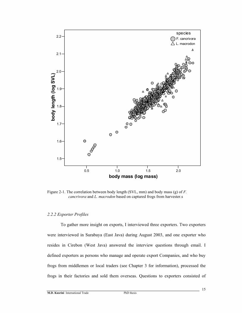
Figure 2-1. The correlation between body length (SVL, mm) and body mass (g) of F. cancrivora and L. macrodon based on captured frogs from harvester.s
2.2.2 Exporter Profiles
To gather more insight on exports, I interviewed three exporters. Two exporters
were interviewed in Surabaya (East Java) during August 2003, and one exporter who
resides in Cirebon (West Java) answered the interview questions through email. I
defined exporters as persons who manage and operate export Companies, and who buy
frogs from middlemen or local traders (see Chapter 3 for information), processed the
frogs in their factories and sold them overseas. Questions to exporters consisted of

M.D. Kusrini International Trade PhD thesis
16
enquires to determine species sold, the seasonality of frog captures, sources of frogs,
countries to which exports were destined, and revenue and problems related to frog
export.
2.3 Results
The earliest data available on frog leg exports are from 1969 as mentioned by
Susanto (1989). Frog legs were listed under fisheries products; from 1969 - 1974 they
were listed simply as frog meat. From 1975 – 1980 they were further categorized as
frog legs, fresh, and chilled/frozen. The number of categories increased further in later
years. The most recent classification of frog legs in the statistical publication is based
on systems first developed in the 1989 Indonesian Tariff Classification, and updated in
1991, 1993 and 1996. Meat from frog sources is now registered under five categories
which are 1: meat and edible meat of frog legs, fresh or chilled, 2: meat and edible meat
of frog legs frozen, 3: meat and edible meat of frogs (excluding legs) fresh or chilled, 4:
meat and edible meat of frogs (excluding legs) frozen, and 5: other meat of frogs.
However, there is no mention of the species from which the meat or legs are taken.
2.3.1 Species exported
Since species taken for export are not recorded in the statistical data, information
on species taken was gathered from interviews with exporters. Interviews revealed that
all companies received frogs from suppliers as skinless frog legs. They usually want
big frogs and accept F. cancrivora, L. macrodon and Rana catesbeiana. One company
actually only accepts L. macrodon, however the manager admitted that since supplies
come in the form of skinless frog legs, as long they are of acceptable size, it is possible
that they include other species such as F. cancrivora.
M.D. Kusrini International Trade PhD thesis
17
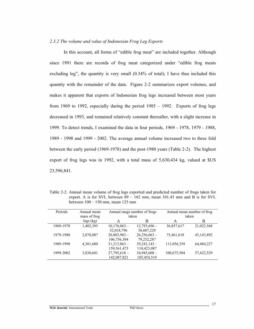
2.3.2 The volume and value of Indonesian Frog Leg Exports
In this account, all forms of “edible frog meat” are included together. Although
since 1991 there are records of frog meat categorized under “edible frog meats
excluding leg”, the quantity is very small (0.34% of total); I have thus included this
quantity with the remainder of the data. Figure 2-2 summarizes export volumes, and
makes it apparent that exports of Indonesian frog legs increased between most years
from 1969 to 1992, especially during the period 1985 – 1992. Exports of frog legs
decreased in 1993, and remained relatively constant thereafter, with a slight increase in
1999. To detect trends, I examined the data in four periods, 1969 - 1978, 1979 - 1988,
1989 - 1998 and 1999 - 2002. The average annual volume increased two to three fold
between the early period (1969-1978) and the post-1980 years (Table 2-2). The highest
export of frog legs was in 1992, with a total mass of 5,630,434 kg, valued at $US
23,596,841.
Table 2-2. Annual mean volume of frog legs exported and predicted number of frogs taken for export. A is for SVL between 89 – 162 mm, mean 101.43 mm and B is for SVL between 100 – 150 mm, mean 125 mm
Annual range number of frogs
taken Annual mean number of frog
taken Periods Annual mean
mass of frog legs (kg) A B A B
1969-1978 1,402,395 10,176,063 –52,018,796
12,793,696 – 38,607,229
36,857,617 21,022,568
1979-1988 2,878,087 20,883,983 –106,756,384
26,256,063 – 79,232,287
75,461,618 43,143,892
1989-1998 4,301,680 31,213,863 – 159,561,473
39,243,143 – 118,423,087
113,056,359 64,484,227
1999-2002 3,830,601 27,795,618 – 142,087,821
34,945,608 – 105,454,519
100,675,504 57,422,529

M.D. Kusrini International Trade PhD thesis
18
Figure 2-2. Volume of frog legs exported by Indonesia from 1969 – 2002. 3 Moving average: A
sequence of averages that are computed from the every three data series to smoothes the fluctuations in data, thus showing the pattern or trend more clearly.
Figure 2-3. Value of frog legs exported by Indonesia from 1969 – 2002. FOB value: value of export
which still included shipping costs and the insurance costs) from the point of manufacture to a specified destination.
Value of Indonesian Frog legs Export from 1969 to 2002
-
5
10
15
20
25
1969
1970
1971
1972
1973
1974
1975
1976
1977
1978
1979
1980
1981
1982
1983
1984
1985
1986
1987
1988
1989
1990
1991
1992
1993
1994
1995
1996
1997
1998
1999
2000
2001
2002
Tota
l val
ue U
S $
Milli
ons
0.0
0.5
1.0
1.5
2.0
2.5
3.0
3.5
4.0
4.5
5.0
aver
age
pric
e/kg
($)
FOB value (US$)Average price/kg ($)
-
1
2
3
4
5
6
1969
1970
1971
1972
1973
1974
1975
1976
1977
1978
1979
1980
1981
1982
1983
1984
1985
1986
1987
1988
1989
1990
1991
1992
1993
1994
1995
1996
1997
1998
1999
2000
2001
2002
Mill
ions
(kilo
gram
s)
year
Net w eight (kg)
3 per. Mov. Avg. (Net w eight (kg))
M.D. Kusrini International Trade PhD thesis
19
As would be expected, the value of frog leg exports has risen with the increase
in volume (Figure 2-3). The average price of frog legs in US$ increased over the period
for which figures were available, with some fluctuations. It was US$ 0.31/kg free on
board (FOB)1 in 1969, and by 2003 it was US$ 3.53/kg .
2.3.3 Destinations of exported frog legs
In total, there are 36 ports of destination for Indonesian frog leg exports. Ten of
these are in countries in Asia (Singapore, Malaysia, Hong Kong, Vietnam, Korea,
China, Japan, Taiwan, Pakistan and East Timor); two are in Middle East countries
(Egypt and Bahrain); 14 are in European countries (Austria, Belgium and Luxembourg,
Bulgaria, Czechoslovakia, Denmark, Finland, France, Germany, Italy, Netherlands,
Spain, Sweden, Switzerland, and United Kingdom; four are in Latin America (Ecuador,
Mexico, Bahamas and Brazil); two are in North America (the USA and Canada) and
four are in Pacific countries (Australia, Papua New Guinea, New Caledonia and other
countries in Oceania). Although Belgium and Luxembourg are different countries, in
the statistical reports they are combined as one entity.
The major importer of Indonesian frog legs is Europe (83.2% of total exports).
Of the European total, Belgium and Luxembourg take the greatest proportion (47.6%),
followed by France (27.6%) and the Netherlands (21%). Eleven other countries in
Europe import frog legs, none taking more than 1% of the European total. In the
earliest period (1969-1980), the main European importer of Indonesian frog legs was
the Netherlands, however, after the 1980s Belgium and Luxembourg dominated the
imports. Exports to Europe tended to fluctuate but increased dramatically after 1985,
1 FOB. A shipping term that indicates that the supplier pays the shipping costs (and usually also the insurance costs) from the point of manufacture to a specified destination, at which point the buyer takes responsibility.

M.D. Kusrini International Trade PhD thesis
20
while exports to Asia tended to increase slightly after 1985 and stabilized around 500
tons annually.
The second largest export destination of Indonesian frog legs is Asia (around
12%). Ten countries in Asia import Indonesian frog legs; the leading importers are
Singapore (50.5% of the Asian total), Hong Kong (22.9%) and Malaysia (18.3%). The
only Asian country that has imported Indonesian frog legs in every year since 1969 is
Singapore. Malaysia has imported continuously since 1981. Two countries in North
America (USA and Canada) currently import small volumes of frog legs from
Indonesia. These countries and apparently did not import from Indonesia during the
1980s.
The results reported above corresponded with those from my interviews. All
exporters reported that most exports go to Europe (Belgium, France, Holland, and
Switzerland) and a small number to the United States and Singapore. They also reported
that demand for frog legs from overseas has been increasing. One manager said that
large increases in demand occurred during the 1980s and since then the market has been
relatively constant, increasing at slow rates compared to the 1980s. Exporters also
reported that they sometimes could not keep up with demand because they are limited
by rates of supply. During February to August (the dry season) supply is usually lower
than during September – January (the wet season).
2.3.4 Frog Exporter Profiles
Companies that export frogs usually also export other fisheries products such as
prawns and fish. In the Ministry of Fisheries report for 2000 there were 22 frog leg
exporting companies listed, employing a total of 3596 people. Almost two thirds (14)
of these companies were based in Java and the rest in Sumatra. This number fluctuates
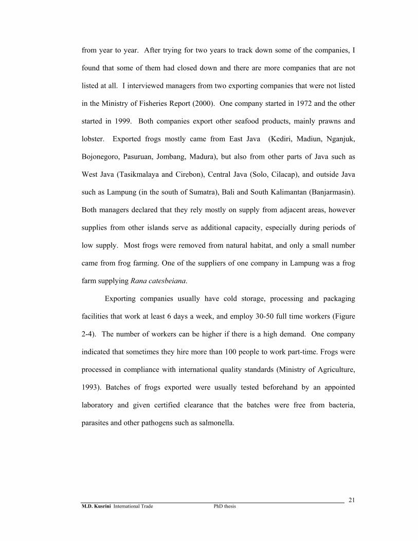
M.D. Kusrini International Trade PhD thesis
21
from year to year. After trying for two years to track down some of the companies, I
found that some of them had closed down and there are more companies that are not
listed at all. I interviewed managers from two exporting companies that were not listed
in the Ministry of Fisheries Report (2000). One company started in 1972 and the other
started in 1999. Both companies export other seafood products, mainly prawns and
lobster. Exported frogs mostly came from East Java (Kediri, Madiun, Nganjuk,
Bojonegoro, Pasuruan, Jombang, Madura), but also from other parts of Java such as
West Java (Tasikmalaya and Cirebon), Central Java (Solo, Cilacap), and outside Java
such as Lampung (in the south of Sumatra), Bali and South Kalimantan (Banjarmasin).
Both managers declared that they rely mostly on supply from adjacent areas, however
supplies from other islands serve as additional capacity, especially during periods of
low supply. Most frogs were removed from natural habitat, and only a small number
came from frog farming. One of the suppliers of one company in Lampung was a frog
farm supplying Rana catesbeiana.
Exporting companies usually have cold storage, processing and packaging
facilities that work at least 6 days a week, and employ 30-50 full time workers (Figure
2-4). The number of workers can be higher if there is a high demand. One company
indicated that sometimes they hire more than 100 people to work part-time. Frogs were
processed in compliance with international quality standards (Ministry of Agriculture,
1993). Batches of frogs exported were usually tested beforehand by an appointed
laboratory and given certified clearance that the batches were free from bacteria,
parasites and other pathogens such as salmonella.
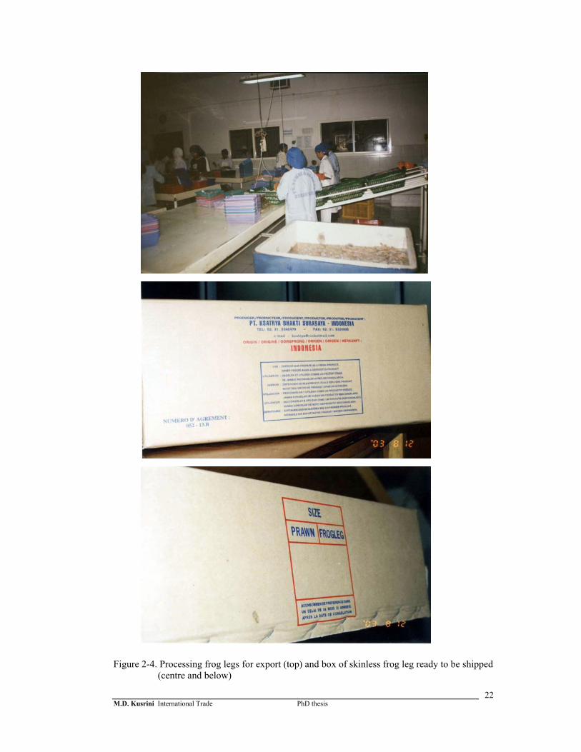
M.D. Kusrini International Trade PhD thesis
22
Figure 2-4. Processing frog legs for export (top) and box of skinless frog leg ready to be shipped
(centre and below)
M.D. Kusrini International Trade PhD thesis
23
2.3.5 The sources of exported frog legs
Export records showed that there are twenty-three ports of exportation. The
ports are situated on five main islands: Java (seven ports), Sumatra (11 ports),
Kalimantan (three ports), Sulawesi (one port) and Bali (one port). Based on the
interviews with exporters, although some frogs originate from other islands, most come
from the island on which the company operates. Since it is difficult to differentiate the
number taken from each province, I assume that frogs originated on the islands on
which exporters are based. On this basis, it is likely that most exported frogs came from
Java and Sumatra (see Figure 2-5). Based on interview data, the majority of frog legs
from Java come from three provinces, Jakarta, Eastern Java and Central Java, and most
frog legs from Sumatra originated in North Sumatra and South Sumatra provinces. The
contribution of frog legs from Sumatra to total exports increased during each period as
the contribution from Java decreased until the period between 1994-1998, however
during 1999 – 2003 the contribution from Java rose again (Figure 2-5).
There are no data regarding whether exported frogs originated from culture or
were removed from natural habitats. The frog culture industry in Indonesia began in
1983 with the introduction of bullfrogs (Rana catesbeiana) as part of an Indonesian
government program to increase frog leg exports (Susanto, 1989; Arie, 1999). In 1999,
the government, through the Ministry of Fisheries, launched a program to increase
fisheries production for export (PROTEKAN) by developing various aspects of
fisheries commodities including freshwater aquaculture by the year 2003. The
freshwater aquaculture industry is primarily directed at three commodities: Tilapia,
frogs and freshwater turtles. Directorate General of Fisheries (DGF, 2001) estimated
that frog culture might produce 1,650 tons per year by the year of 2003. Based on this

M.D. Kusrini International Trade PhD thesis
24
amount, it appears that most exported frogs have been, and will continue to be, removed
from natural habitats.
Figure 2-5. The volume of frog legs exported out of ports in four main islands in Indonesia
A discussion with staff from Balai Budidaya Air Tawar (the Centre for
Freshwater Aquaculture) in Sukabumi, West Java on October 2001 also revealed that
many farmers had stopped culturing Rana catesbeiana because of high maintenance
costs and disease. This was confirmed by an interview with one of the frog farmers in
East Java. This indicates that frog culture is unlikely to contribute substantially to
future exports.
2.3.6 Number harvested for export
The mean number of frogs exported annually during 1989-1998 is estimated in
the range of 31 – 160 millions frogs per year, depending on the length of frogs used in
the equations (Table 2-2). However, the actual number of frogs taken was probably
-
2
4
6
8
10
12
14
16
1969-1973 1974-1978 1979-1983 1984-1988 1989-1993 1994-1998 1999-2003
year
tota
l fro
g le
gs v
olum
e (m
illio
ns k
g)Sumatra
Java
Kalimantan
Sulaw esi

M.D. Kusrini International Trade PhD thesis
25
higher than recorded. Exporters will only take frog legs that have no bruises or other
imperfections. Because frogs are usually captured using a net on a long pole, some are
inevitably bruised, and the number of frogs rejected by exporters varied from 2 - 5% of
the total frogs caught, although one middlemen remarked that he had once rejected as
much as 30% (Chapter 3). Rejected frogs are sometimes thrown away because some
domestic markets prefer live frogs (Chapter 3).
2.4 Discussion
Previous authors have reported that the common edible frogs of Indonesia
consist of Fejervarya cancrivora, F. limnocharis, L. macrodon, and the introduced
species Rana catesbeiana (Church, 1960; Berry, 1975; Iskandar, 1998; Susanto, 1989).
The problem of identifying the species exported lies in the fact that frogs are usually
exported as skinless frog legs. Even if species were identified, the documentation in
export papers could be incorrect. For example, Veith et al. (2000) performed DNA
analyses to compare imported frog legs from Java and Sumatra with frozen tissues of
Indonesian Ranid species. Their results showed that samples of tissue that had been
documented as belonging to the species L. macrodon, F. cancrivora, F. limnocharis,
and R. catesbiana, were all in fact F. cancrivora.
Exported Fejervarya cancrivora and L. macrodon are usually taken from the
wild. Previous studies have suggested that Fejervarya cancrivora is the most common
species in rice fields, a habitat mostly associated with humans (Church; 1960; Alcala,
1962; Berry, 1975; Iskandar, 1998). Limnonectes macrodon is thought to live mostly
near rivers or in small streams (Iskandar, 1998) but in my fieldwork this species was
also found in ponds and rice fields (see Chapter 4). Both are large species and are found
M.D. Kusrini International Trade PhD thesis
26
in areas accessible to harvesters, therefore they are probably the most caught for export
purposes, especially in Java.
It is not clear from the statistical records what species are taken for the frog leg
trade and in what numbers they are taken; these need to be assessed for management
purposes. The species that are harvested are likely to differ among locations. As an
archipelago, Indonesia consists of several main islands, and each island has its own
unique faunal assemblage. It is likely that outside Java, species other than F.
cancrivora and L. macrodon are taken. Exporters that use supplies from other islands
usually record only the names of locally available species (e.g. kodok lembu, the local
name for Rana catesbeiana or kodok batu, the local name for Limnonectes macrodon).
Since the frogs taken must be of similar size to L. macrodon, it is possible that species
captured from other islands may be other members of the genus Limnonectes.
Data show that the numbers of frogs caught for export purposes increased
significantly between the first period (1969 - 1979) and the second period (1979 - 1988)
for which data were available. Before 1985, India and Bangladesh were the main global
sources of exported frog legs. However, in 1985 their two edible frog species
(Euphyctis hexadactylus and Holobatrachus tigerinus) were included in Appendix II of
CITES (the Convention on International Trade in Endangered Species of Wild Fauna
and Flora), because of declines in their populations (Abdulali, 1985; Pandian and
Marian, 1986; Dash and Mahanta, 1993). A comparison of Indonesian, Indian, and
Bangladeshi frog leg export data (Schmuck 2000a) suggested that Indonesian exports
rose markedly as exports from Bangladesh and India decreased.
Although some exported frogs were probably transported between islands, it is
likely that almost all exported frogs originated on the island where each exporting
company resides. Even if we assume that up to 20% of frogs from Java could have
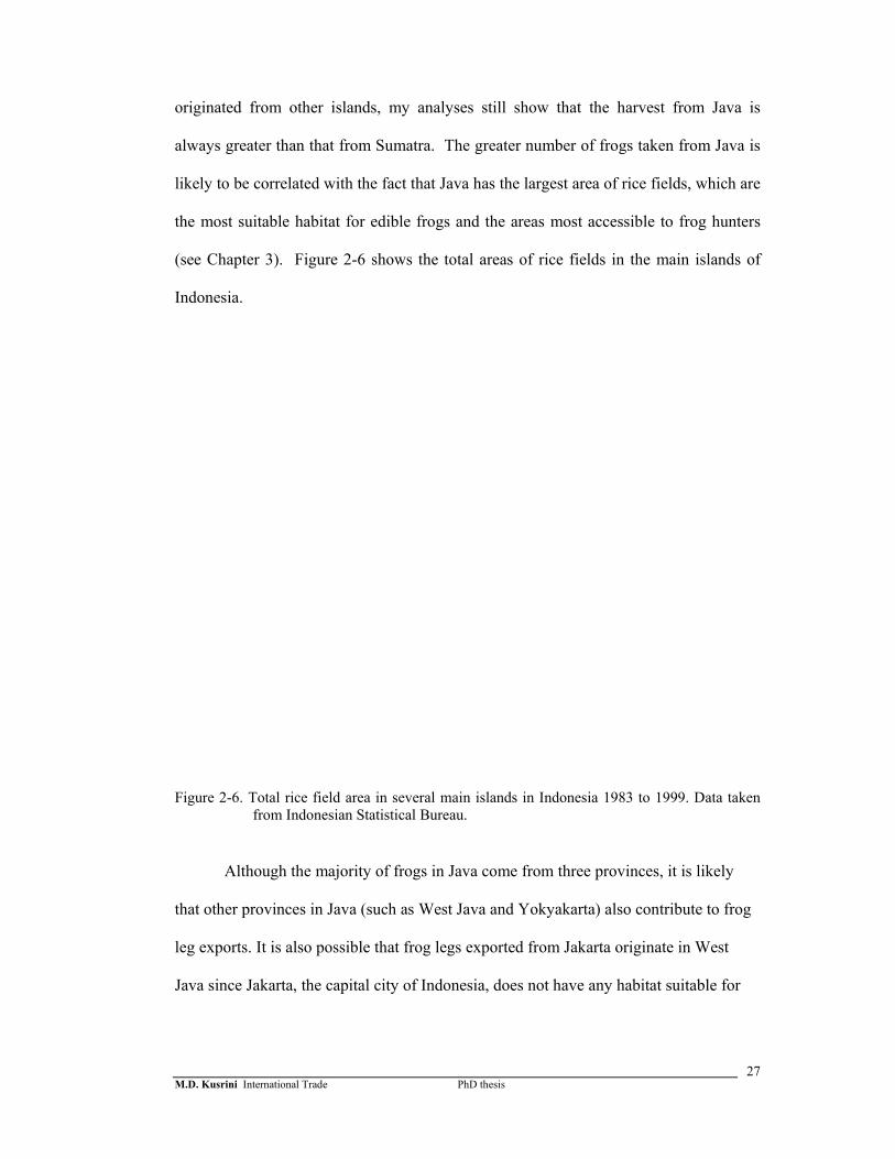
M.D. Kusrini International Trade PhD thesis
27
originated from other islands, my analyses still show that the harvest from Java is
always greater than that from Sumatra. The greater number of frogs taken from Java is
likely to be correlated with the fact that Java has the largest area of rice fields, which are
the most suitable habitat for edible frogs and the areas most accessible to frog hunters
(see Chapter 3). Figure 2-6 shows the total areas of rice fields in the main islands of
Indonesia.
Figure 2-6. Total rice field area in several main islands in Indonesia 1983 to 1999. Data taken from Indonesian Statistical Bureau.
Although the majority of frogs in Java come from three provinces, it is likely
that other provinces in Java (such as West Java and Yokyakarta) also contribute to frog
leg exports. It is also possible that frog legs exported from Jakarta originate in West
Java since Jakarta, the capital city of Indonesia, does not have any habitat suitable for

M.D. Kusrini International Trade PhD thesis
28
edible frogs, and also Jakarta is the nearest major port to West Java. A small fraction of
frog legs from West Java might also go through Central Java.
The major importer of Indonesian frog legs in Europe is Belgium and
Luxembourg (47.6%), followed by France (27.6%) and the Netherlands (21%). This
contradicts the idea that France is the major importer of Indonesian frog legs (Patel,
1993). However, Belgium and Luxembourg could also serve as gateways to Europe;
from these ports of entry frog legs may be re-exported to other European countries.
My data suggested that the number of frogs taken for export purposes is high
(see Table 2-2). Data from India suggested that the number taken for export before the
ban was around 60 million/year (Pandian and Marian, 1986). Although my estimated
number of Indonesian frog harvested is larger than this number, this does not
necessarily mean that the Indonesian species are threatened by harvesting. They differ
in breeding regimes, environmental condition, and available area of habitat.
Besides export, the domestic sector also utilises frogs. Although most
Indonesians are Moslems, and thus are forbidden to eat frogs, ethnic Chinese and
persons of other religions may consume large numbers of frog legs. There are no data
available on the volume of frog legs used for domestic consumption. The volume of
frogs harvested for domestic consumption is analysed more thoroughly in Chapter 3.
_________________________________________________________________________________ M.D. Kusrini Edible frog harvesting PhD Thesis
29
CHAPTER 3
EDIBLE FROG HARVESTING AND THE STRUCTURE OF THE DOMESTIC
MARKET
3.1 Introduction
Issues regarding the sustainability of game harvests in various tropical forests
have been assessed thoroughly by Robinson and Bennett (2000). From this book it is
clear that to conserve harvested species, researchers cannot focus only on the ecology
and biology of those but also need to examine the human aspects of harvests. In the
case of the Indonesian frog harvest the questions that must be addressed are: What is the
importance of this harvest? Where does the harvest go? What methods do hunters use to
catch the frogs? Will the methods used to catch frogs be detrimental to non-target
species? By addressing the human aspects of the harvest we can also get a clearer
picture of harvest rates and other issues related to the survival of the harvested species,
such as whether the frog harvest is seasonal and whether it is size selective.
Unfortunately, most authors who have dealt with the issue of frog harvesting
have neglected the human dimension. Pandian and Marian (1986) briefly mentioned
that the ban on Indian frog leg exports resulted in the collapse of this industry and the
loss of jobs for many people. This chapter examines these human dimension issues with
data on the harvesting and marketing of edible frog legs in Jakarta, West Java and East
Java with an emphasis on domestic frog supply.
3.2 Methods
I defined three occupational categories related to frog harvesting. Frog hunters
or harvesters are defined as people whose main activity is the actual harvesting of frogs.
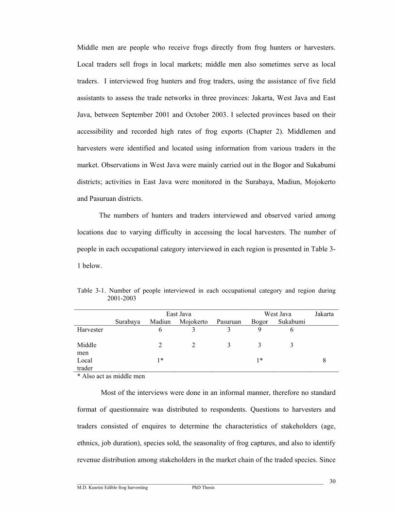
_________________________________________________________________________________ M.D. Kusrini Edible frog harvesting PhD Thesis
30
Middle men are people who receive frogs directly from frog hunters or harvesters.
Local traders sell frogs in local markets; middle men also sometimes serve as local
traders. I interviewed frog hunters and frog traders, using the assistance of five field
assistants to assess the trade networks in three provinces: Jakarta, West Java and East
Java, between September 2001 and October 2003. I selected provinces based on their
accessibility and recorded high rates of frog exports (Chapter 2). Middlemen and
harvesters were identified and located using information from various traders in the
market. Observations in West Java were mainly carried out in the Bogor and Sukabumi
districts; activities in East Java were monitored in the Surabaya, Madiun, Mojokerto
and Pasuruan districts.
The numbers of hunters and traders interviewed and observed varied among
locations due to varying difficulty in accessing the local harvesters. The number of
people in each occupational category interviewed in each region is presented in Table 3-
1 below.
Table 3-1. Number of people interviewed in each occupational category and region during
2001-2003
East Java West Java Surabaya Madiun Mojokerto Pasuruan Bogor Sukabumi
Jakarta
Harvester
6 3 3 9 6
Middle men
2 2 3 3 3
Local trader
1* 1* 8
* Also act as middle men Most of the interviews were done in an informal manner, therefore no standard
format of questionnaire was distributed to respondents. Questions to harvesters and
traders consisted of enquires to determine the characteristics of stakeholders (age,
ethnics, job duration), species sold, the seasonality of frog captures, and also to identify
revenue distribution among stakeholders in the market chain of the traded species. Since
_________________________________________________________________________________ M.D. Kusrini Edible frog harvesting PhD Thesis
31
there are no previous data on sizes of populations of edible frogs, to obtain information
on the fluctuations of the harvest we also asked harvesters whether the harvest has been
lower in recent years. To assess the size classes preferred by harvesters and traders,
frogs caught by harvesters (usually harvesters who had been followed by my team) were
measured for their snout vent length and mass. The results are presented in a descriptive
manner.
In addition, in 2001 I also interviewed a researcher from Balai Budidaya Air
Tawar or BBAT (Fresh Water Aquaculture Research) in Sukabumi, an institution that
was responsible for culturing the bullfrog (Rana catesbeiana) the first time. A bullfrog
farmer in East Java was also interviewed during August 2003 to gain information on the
problems associated with, and extent of development of, frog farms.
Local markets in each area were also surveyed to record the species and
numbers of frogs sold. The market surveys were carried out discreetly or openly
depending on the situation. A discreet survey was carried out if it would be likely to
upset the traders; in Indonesia that means attracting a large crowd which would make
working very difficult. The data were either recorded directly into a small hidden tape
recorder or memorized by the investigators and put onto record sheets a short distance
away from the market stall.
To calculate harvesting rates in local areas, data were collected by following 10
frog hunters across all of the local area (West Java and East Java) for an overall total of
21 night works. Routes were recorded with GPS to obtain information such as working
hours per days and the size of search areas. From this data I estimated catch per hunter-
night of effort for each area.
By obtaining data on actual harvesting rates, I could estimate the proportions of
frogs taken for domestic consumption and for export. I calculated the proportion of

_________________________________________________________________________________ M.D. Kusrini Edible frog harvesting PhD Thesis
32
frogs suitable for export as the proportion that were of sizes suitable for export (mass >
80 grams); frogs below this size must be destined for domestic consumption.
3.3 Results
3.3.1. Species harvested
a. Species in trade
Four species of frogs were sold in local markets: Fejervarya cancrivora,
Fejervarya limnocharis-iskandari complex, Limnonectes macrodon and Rana
catesbeiana. Of the local species, the larger species (F. cancrivora and L. macrodon)
were sold the most. Surveys in East Java only found two species being traded: F.
cancrivora and F. limnocharis-iskandari complex. However, East Java traders did say
that they sometimes sold stream frogs matching the description of L. macrodon.
Fejervarya limnocharis-iskandari complex were not only sold as for human
consumption but also as fish bait. We rarely saw Rana catesbeiana in local markets,
however a few supermarkets in Jakarta such as Ranch 99 sold them. Interviews with
local traders in all markets revealed that most local consumers dislike the taste of R.
catesbeiana and prefer local frogs.
In West Java and Jakarta’s local markets F. cancrivora and L. macrodon were
usually sold by number rather than by weight, whereas in East Java F. cancrivora were
sold by weight (whole) (Figure 3-1). Local consumers selected frogs whilst they were
still alive. The trader either delivered them to the consumer alive or cut and skinned the
legs before delivering them.
Small frogs such as F. limnocharis-iskandari complex are either sold alive by
number for fish bait or are sold by weight as skinless frog legs. Local markets usually
demand live frogs for sale; as such, the outward appearance of frogs is important.
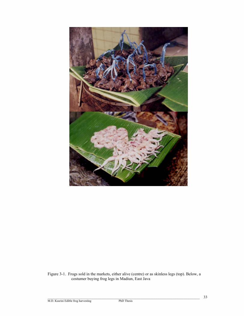
_________________________________________________________________________________ M.D. Kusrini Edible frog harvesting PhD Thesis
33
Figure 3-1. Frogs sold in the markets, either alive (centre) or as skinless legs (top). Below, a costumer buying frog legs in Madiun, East Java

_________________________________________________________________________________ M.D. Kusrini Edible frog harvesting PhD Thesis
34
b. Frog sizes
A total of 736 frogs of three species (Fejervarya cancrivora, F. limnocharis-
iskandari complex and L. macrodon) captured by harvesters were measured. Most of the
frogs captured were F. cancrivora (75.4%), while only a small percentage were F.
limnocharis-iskandari complex (5.8%) and the rest were L. macrodon. Frogs captured
were usually mature, except for F. cancrivora where a small number of captured
individuals were of sizes considered to be juveniles (see Chapter 5 for the description of
sex differentiation for F. cancrivora and F. limnocharis-iskandari complex). The mean
SVL of F. cancrivora captured was 71.50 mm and mean mass was 41.88 grams. The
means for F. limnocharis-iskandari complex were 45.29 mm and 10.67 grams,
respectively, and those for L. macrodon were 80.47 mm and 66.41 grams (Table 3-2).
Table 3-2. Size and Mass of Frogs captured by harvesters; F = female, M = male and J = juvenile
SVL (mm) Mass (gram) Species Sex N Mean Range Std
Dev Mean Range Std
Dev F 367 75.10 40.00 -162.00 16.89 48.55 2.94 - 152.40 26.48 J 5 35.90 33.50 - 38.00 1.75 3.93 3.45 - 4.35 0.35
M 183 65.54 50.20 - 86.20 6.01 29.55 14.50 - 57.40 8.09
Fejervarya cancrivora
Total 555 71.60 33.50 - 162.00 15.23 41.88 2.94 - 152.40 24.03 F 16 43.69 30.00 - 78.00 16.22 10.34 1.87 - 32.00 12.9 M 27 46.24 32.57 - 70.20 13.75 10.87 2.60 - 41.00 10.04
Fejervarya limnocharis-iskandari complex Total 43 45.29 30.00 - 78.00 14.58 10.67 1.87 - 41.00 11.04 Limnonectes macrodon 138 80.47 54.74 -138.10 12.78 66.41 17.00 - 146.05 26.49
3.3.2 The process of harvesting frogs and the characteristics of harvesters a. Profiles of harvesters, middle men and traders
Frog harvesting is a nocturnal job, therefore it is not surprising that all frog
harvesters are males. Harvesters’ ages are variable, ranging from 25 to 60 years old. The
maximum length of time of employment in this work was around 30 years. More than
_________________________________________________________________________________ M.D. Kusrini Edible frog harvesting PhD Thesis
35
one third of the harvesters (37%) had worked for more than 20 years, nine people (33
%) had worked between 10-20 years, six people had worked (22%) between 5-10 years,
and only two people (7%) had worked for less than five years. More than half (56%)
worked part-time as frog hunters. During the day they worked as farmers, farm
labourers, general labourers, brick makers, public transportation drivers or as middle
men. All harvesters were local people, meaning that they live near the place where they
capture and sell frogs. East Javan harvesters were either Maduranese (Madura is a
nearby small island in the north coast of East Java) or East Javanese. All West Javan
harvesters were Sundanese (Sunda is an ethnic group from West Java). Some of the
harvesters were related (brothers or father and sons) to other harvesters or middle men.
Full time harvesters usually work nearly every night, taking time off at least once a
week and during the full moon. Part-time harvesters usually work only during the high
season.
Three middle men were female and the rest were males. Half of the middle men
had worked more than five years, 29% had worked for 10-20 years whilst 21% had
worked more than 20 years. Four male middle men started their careers as harvesters.
One of the middle men from Sukabumi worked as a harvester from the 1950s to the
1970s. He could not remember the exact dates, and used certain historical events as his
time marks. In this case he started working as a harvester during the Darul
Islamiyah/Tentara Islam Indonesia Rebellion (around 1955) and finished working as a
harvester not long after the Communist Party was disbanded (the late 1960s).
Harvesters usually “belong” to (work exclusively with) one of the middle men.
They are given upfront money by middle men, usually for transportation, and have to
give all of their harvest to their middle man. Middle men also loan equipment, such as
carbide lamps, bags and capture devices, to harvesters. They also sometimes provide
_________________________________________________________________________________ M.D. Kusrini Edible frog harvesting PhD Thesis
36
food or a cup of coffee to harvesters before and after work. However, the loyalties of
harvesters usually depend on the price of frogs given by the middle men. The number of
harvesters working for one middle man varied; usually between 5 – 40 people each day
depending on the season. In the high season the number of harvesters working was
usually higher than in the low season. The low season usually occurs during the full
moon and in the dry season.
Some of the middle men not only sent their frogs to other distributors or traders
but also act as traders in local markets. Most traders had worked more than five years
and some “inherited” the work from relatives.
b. Harvesting Techniques
Harvesters use lights powered by carbide or batteries to help them capture frogs.
This has led to their occupation being called pengobor (West Java) or penyuluh (East
Java), which literally means men who use torches. To capture frogs, most harvesters
walk in or along areas of frog habitat such as rice fields, small fish ponds, ponds inside
forested areas, and irrigation ditches near sugar cane or riversides. Only one harvester
from Sukabumi indicated he used a dinghy when cruising the river Cikarang to find
frogs. The total distance traversed during searches was up to 10 km/night. Working time
usually started around 7.00 p.m. and finished around 1.00 a.m. The route taken was
rarely far from their home or from their middle man’s area; this minimizes travel costs.
Harvesters used active hunting techniques in which frogs were captured using
special equipment: a long bamboo pole with a net at the end (West Java) or a long
bamboo pole with a three-headed spear (East Java) (Figure 3-2). This long pole helps
harvesters to capture frogs that are a bit far from where the harvester is standing.
Sometimes frogs hide in crevices; this is where the three-headed spear becomes useful
_________________________________________________________________________________ M.D. Kusrini Edible frog harvesting PhD Thesis
37
to capture hidden frogs. Harvesters usually tried to avoid spearing frogs in their legs
because the resulting bruises would cause their rejection, especially for export purposes.
However, sometimes it is difficult to avoid such bruising, especially when frogs are
hiding (Figure 3-3). Captured frogs are put in special bags. West Javan harvesters
avoided frog mortality during capture because frogs were usually sold live, whereas it
did not matter to East Javan harvesters whether frogs were alive or dead, since as soon
as their middle men weighed their catch, the frogs’ legs were removed and skinned.
Most harvesters work alone. They occasionally worked in pairs when one was
new at the work. As soon as a new harvester had learned the techniques, he would work
alone. One harvester from Sukabumi worked with a team of 2-4 people during the times
when he used a dinghy in the Cikarang River; at other times he worked alone.
c. Harvesting effort
Before going to work, harvesters usually assembled in their middle men’s
houses to prepare their equipment and determine the route to be taken that day. They
usually started to work after 7 p.m. by going to the starting point of their selected route
either by foot or public transportation. The mean total time spent by harvesters in
traversing their routes was 17948.52 seconds or 4 hours 59 minutes and 8.52 seconds.
The starting point was taken as the point at which harvesters began searching for frogs.
Along the way, they sometimes rested for snacks or coffee for between 10-15 minutes
and one hour. The number of frogs caught ranged from six to 110 frogs, with total wet
masses from 508.8 – 5000 grams. Mean catch per unit effort was 8.74 frogs/hour (range
1.79 – 20.50 frogs/hour) or 351.32 grams/hour (range 94.65 – 931.68 grams/hour).
Table 3-3 shows the number and mass of frogs captured for each trip for each harvester.

_________________________________________________________________________________ M.D. Kusrini Edible frog harvesting PhD Thesis
38
Based upon interviews, during the full moon or the dry season, yields were
usually between 1 - 2 kg/harvester/night whereas during the wet season the yield can be
between 2 – 5 kg/harvester/night. Several harvesters in West Java counted the yield not
by mass but by number. Based on interviews the numbers of frogs caught per day were
usually between 30-40 frogs during the low season and 70 – 100 frogs during the high
season.
Table 3-3. The average trip length and catch/effort per hour and per km of harvester
East Java (n=6 days)
West Java (n = 15 days)
Total (n= 21 days)
Average length of Trip (km) 10.80 9.76 10.06 Range 9.46 -12.18 5.07 - 16.00 5.07 - 16.00 SD 1.12 3.29 2.85 Average of Total times (seconds) 19742.17 17231.07 17948.52 Range 17168 - 24691 12073 - 22860 12073 - 24691 SD 2764.35 3347.17 3332.28 Average of Catch/effort (g/hour) 395.28 332.38 351.32 Range 325.71 - 505.13 94.65 - 931.68 94.65 - 931.68 SD 67.71 239.55 203.32 Average of Catch/effort (n/hour) 11.37 7.42 8.74 Range 8.23 - 15.67 1.79 - 20.50 1.79 - 20.50 SD 2.53 5.73 5.17 Average of Catch/effort (g/km) 203.41 165.15 176.63 Range 156.01 - 289.19 50.00 - 349.65 50.00 - 349.65 SD 54.63 105.10 93.10 Average of Catch/effort (n/km) 5.86 3.86 4.53 Range 3.94 - 8.96 0.83 - 9.40 0.83 - 9.40 SD 1.83 2.51 2.45
3.3.3. Market structure
The market structure for wildlife trades can be either competitive or
monopolistic (Clayton and Millner-Gulland, 2000). The local frog leg trade follows the
classic chain of marketing which includes three to four main stakeholders: harvesters,
middle men, suppliers and traders (Figure 3-4). In competitive markets, each
stakeholder can enter or leave the market freely while in monopolistic markets, access is
controlled and denied by various means such as ownership or law enforcement (Clayton
and Millner-Gulland, 2000).
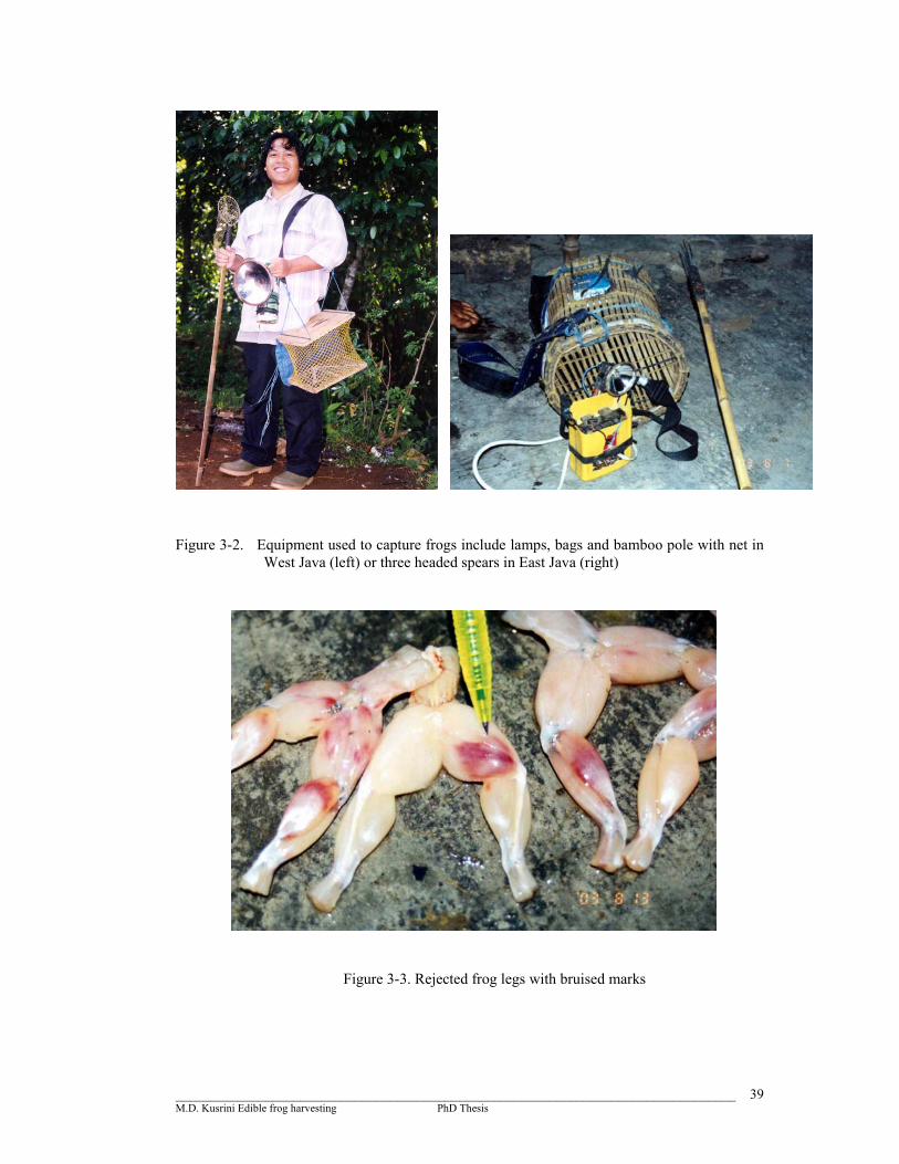
_________________________________________________________________________________ M.D. Kusrini Edible frog harvesting PhD Thesis
39
Figure 3-2. Equipment used to capture frogs include lamps, bags and bamboo pole with net in West Java (left) or three headed spears in East Java (right)
Figure 3-3. Rejected frog legs with bruised marks
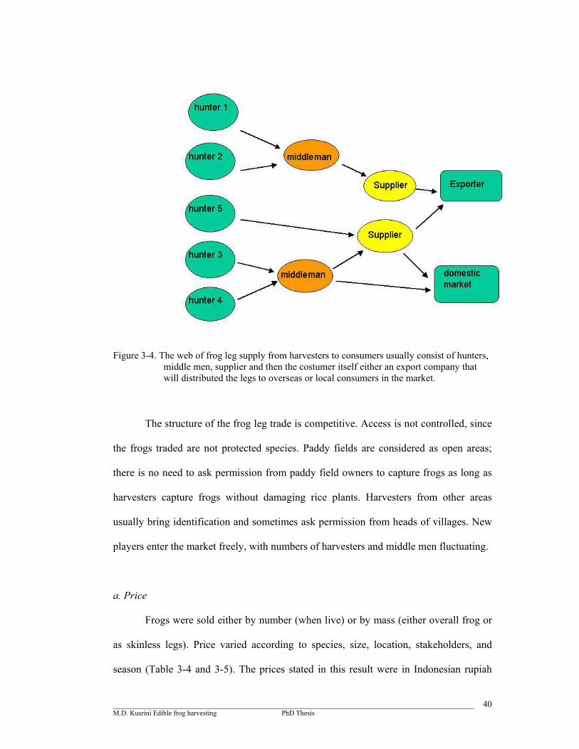
_________________________________________________________________________________ M.D. Kusrini Edible frog harvesting PhD Thesis
40
Figure 3-4. The web of frog leg supply from harvesters to consumers usually consist of hunters, middle men, supplier and then the costumer itself either an export company that will distributed the legs to overseas or local consumers in the market.
The structure of the frog leg trade is competitive. Access is not controlled, since
the frogs traded are not protected species. Paddy fields are considered as open areas;
there is no need to ask permission from paddy field owners to capture frogs as long as
harvesters capture frogs without damaging rice plants. Harvesters from other areas
usually bring identification and sometimes ask permission from heads of villages. New
players enter the market freely, with numbers of harvesters and middle men fluctuating.
a. Price
Frogs were sold either by number (when live) or by mass (either overall frog or
as skinless legs). Price varied according to species, size, location, stakeholders, and
season (Table 3-4 and 3-5). The prices stated in this result were in Indonesian rupiah

_________________________________________________________________________________ M.D. Kusrini Edible frog harvesting PhD Thesis
41
(Rp) for the years 2002 and 2003. The price of Limnonectes macrodon was usually
higher than that for rice field frogs. In West Java and Jakarta it is usually sold live by
number or by weight. Harvesters sold this frog for Rp. 750/frog or Rp. 5000 – 14000/kg
to middle men. The cheapest L. macrodon sold to consumers was in Bogor (Rp.
1250/frog) compared to Jakarta, where prices ranged from Rp. 1500 (small) to Rp. 3000
(large)/frog, or around Rp. 25000/kg.
The prices of rice field frogs varied according to size and location. There were
no standard categories, however traders usually categorized frogs into large, medium or
small. Some traders categorized frogs using an alphabetical system: A, B and C.
Categories A and B are large and medium frogs, with 9-12 frogs/kg (A), or 13- 25
frogs/kg (B) whereas more than 25 frogs/kg were categorized as C or small. The price
per individual and per kilogram was lower for smaller frogs. The price of frogs usually
increased 2-3 times from harvester to local consumer (Table 3-4). Frog legs exported
are usually from large frogs (category A or B) with prices in year 2003 around US$ 3-
4/kg of skinless frog legs or around Rp. 25,200 – 33,600/kg with a currency exchange
rate of 1 US$ = Rp. 8,400.
b. Levels of Income and Profit
Harvester income depends on the number or mass of frogs caught, route taken
and skills. To minimize costs of transportation, harvesters rarely go far from the place
where they sell the catch, preferring to walk whenever possible. Other than
transportation, additional costs for each trip were for snacks, coffee and cigarettes. The
maximum cost of transportation and snacks (including coffee and cigarettes) along the
way that harvesters were willing to spend was Rp 1,000/day during high season. If we
assume that transportation cost is nil and the price of frogs is constant at Rp. 6000/kg
(mixed), harvesters could make around Rp. 5,000-11,000/ day (low season) and Rp.

_________________________________________________________________________________ M.D. Kusrini Edible frog harvesting PhD Thesis
42
11,000 to 29,000/day (high season) (Table 3-7). A full time harvester working for 25
days/month would receive a monthly income of Rp. 245,000 to 635,000. This estimate
is probably lower than actual earnings, because harvesters tend to capture bigger frogs
(thus increasing their income) and prices fluctuate, and are higher in the low season
because of lower supply. Based on interviews, the lowest income of a full time
harvester was Rp. 450,000/month whilst the highest was 900,000/month.
For middle men, the gross revenue for each type of frog varied (see Table 3-4
and 3-5). Middle men and traders must also spend substantial amounts of money for
fixed costs such as equipment, carbide or batteries, transportation to carry frogs to
traders or local markets, and hiring people to cut and skin frogs. Middle men who had
connections with exporters usually did not need to cover the costs of transportation
since exporters usually come to the middle man. However, interviews revealed that only
some middle men distributed their frog legs to exporters. Exporters usually have higher
quality control. Interviews with exporters revealed that at least 2-5% of frog legs
coming from middle men were usually rejected for various reasons such as the
occurrence of bruises or parasite infection. One of the middle men interviewed
remarked that he had lost a substantial amount of money because more than 30% of the
last batch of frog legs he sent was rejected. This caused him to leave the export market
and concentrate on the local market, which he said was much more flexible. Other
middle men used other approaches, catering for both local and export markets. Frogs
that are too small for export are sold in local markets. Net revenue for middle men and
traders varies, ranging from Rp.100,000/day to Rp. 600,000/day.

_________________________________________________________________________________ M
.D. K
usrini Edible frog harvesting PhD
Thesis 43
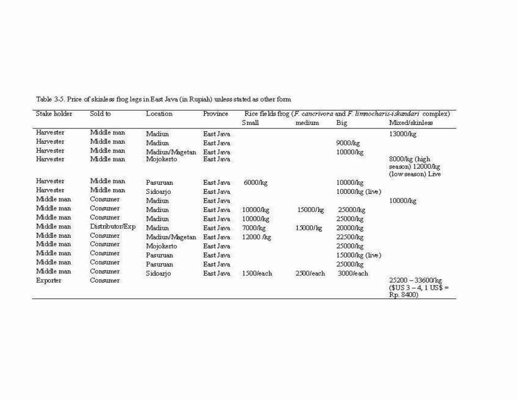
_________________________________________________________________________________ M
.D. K
usrini Edible frog harvesting PhD
Thesis 44
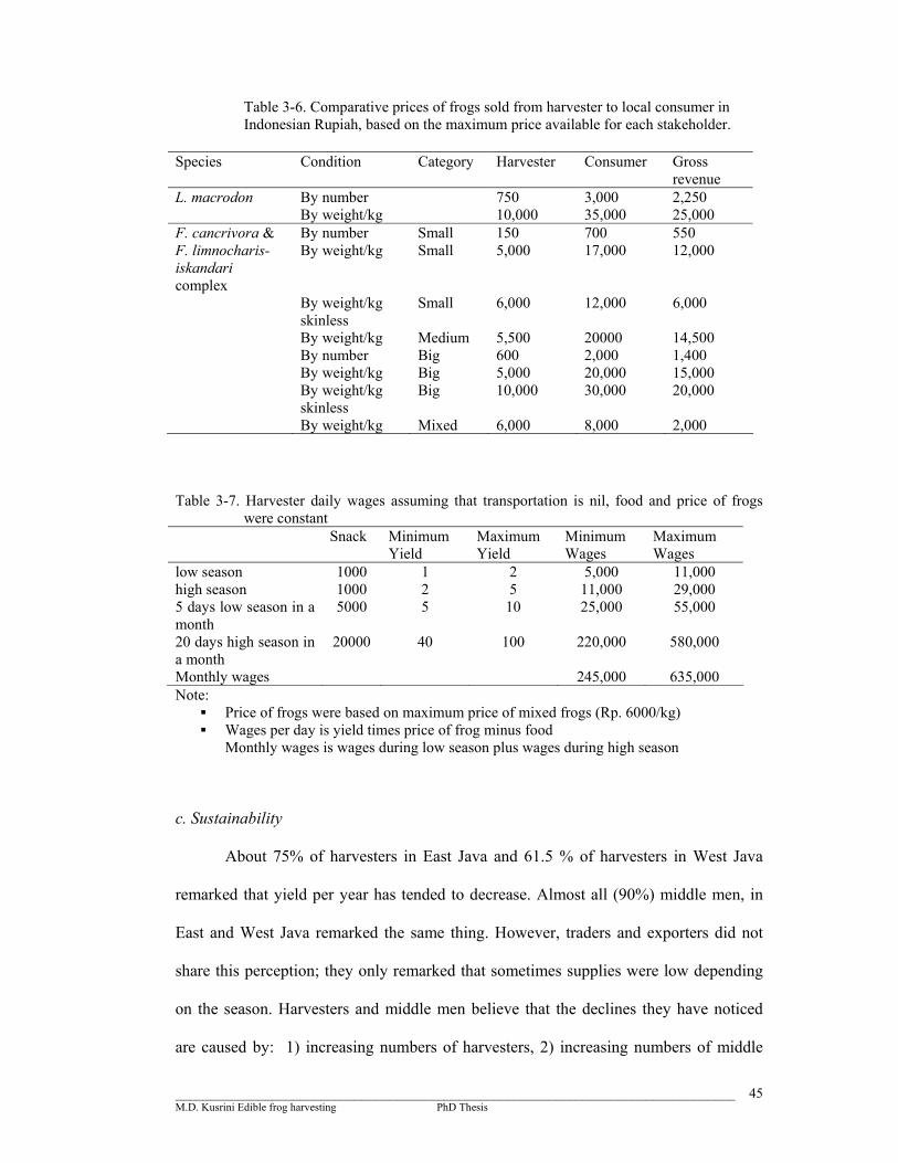
_________________________________________________________________________________ M.D. Kusrini Edible frog harvesting PhD Thesis
45
Table 3-6. Comparative prices of frogs sold from harvester to local consumer in Indonesian Rupiah, based on the maximum price available for each stakeholder.
Species Condition Category Harvester Consumer Gross
revenue L. macrodon By number 750 3,000 2,250 By weight/kg 10,000 35,000 25,000 F. cancrivora & By number Small 150 700 550 F. limnocharis-iskandari complex
By weight/kg Small 5,000 17,000 12,000
By weight/kg skinless
Small 6,000 12,000 6,000
By weight/kg Medium 5,500 20000 14,500 By number Big 600 2,000 1,400 By weight/kg Big 5,000 20,000 15,000 By weight/kg
skinless Big 10,000 30,000 20,000
By weight/kg Mixed 6,000 8,000 2,000
Table 3-7. Harvester daily wages assuming that transportation is nil, food and price of frogs were constant
Snack Minimum Yield
Maximum Yield
Minimum Wages
Maximum Wages
low season 1000 1 2 5,000 11,000 high season 1000 2 5 11,000 29,000 5 days low season in a month
5000 5 10 25,000 55,000
20 days high season in a month
20000 40 100 220,000 580,000
Monthly wages 245,000 635,000 Note:
Price of frogs were based on maximum price of mixed frogs (Rp. 6000/kg) Wages per day is yield times price of frog minus food
Monthly wages is wages during low season plus wages during high season
c. Sustainability
About 75% of harvesters in East Java and 61.5 % of harvesters in West Java
remarked that yield per year has tended to decrease. Almost all (90%) middle men, in
East and West Java remarked the same thing. However, traders and exporters did not
share this perception; they only remarked that sometimes supplies were low depending
on the season. Harvesters and middle men believe that the declines they have noticed
are caused by: 1) increasing numbers of harvesters, 2) increasing numbers of middle

_________________________________________________________________________________ M.D. Kusrini Edible frog harvesting PhD Thesis
46
men, allowing harvesters to go to other middle men, and 3) habitat change, as more rice
fields have been developed for other uses. Very few respondents suggested that the
decreased numbers of frogs captured were caused by decreases in frog populations. An
account by one of the middle men from Sukabumi who had worked as a harvester in the
1950s through –1970s suggested that some frog populations may have decreased. In
West Java more stream frogs than rice field frogs were captured in the 1960s. During
the 1970s the number of stream frogs captured decreased and the harvester shifted his
capture efforts to rice field frogs. During the 1970s, a one-day yield for one middle man
could consist of a maximum of 200-500 kilograms of frogs. Nowadays, with almost the
same number of harvesters he can only obtain a maximum 100 to 200 kilograms for 3
days work or about 33 – 66 kg/day, which is a substantial decrease.
One approach to reducing the impact of harvesting on natural frog populations is
to farm frogs. Although bullfrogs (Rana catesbeiana) were introduced as early as 1983
for frog farming purposes (Susanto, 1989; Iskandar, 1998; Arie, 1999), so far, the frog
farming industry in Indonesia has not developed as expected. An interview with a
research aquaculturist from BBAT revealed that attempts at frog farming have usually
been short lived. Many frog farmers have abandoned their attempts due to the expense
of food and maintenance. These factors were also mentioned by an ex- frog farmer
interviewed in Surabaya (Figure 3-5).
d. Number of frogs sold in local market
In contrast to frog leg exports (Chapter 2), no data are available on the local
trade in frog legs. Because the majority of the Indonesian population are Muslims (85%
based on the 2002 census), who are forbidden to eat frogs, frog legs are not a major
food for Indonesians. However, if most of the remaining 15% of the 234 million people
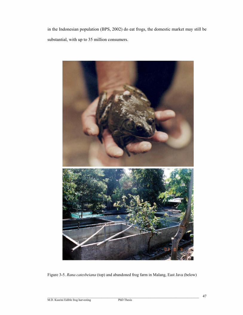
_________________________________________________________________________________ M.D. Kusrini Edible frog harvesting PhD Thesis
47
in the Indonesian population (BPS, 2002) do eat frogs, the domestic market may still be
substantial, with up to 35 million consumers.
Figure 3-5. Rana catesbeiana (top) and abandoned frog farm in Malang, East Java (below)

_________________________________________________________________________________ M.D. Kusrini Edible frog harvesting PhD Thesis
48
Determining the total extent of the frog leg trade in local markets is very
difficult, because the number of markets is not known; nor is the number of sellers. For
example, my survey found at least 15 local markets in Jakarta selling frog legs,
excluding supermarkets. Since the export market uses large frogs (Category A,
maximum 12 frogs/kg wet weight, each frog ~ 80 gram) almost exclusively, the
proportion of captured frogs that enter local markets can be estimated as the proportion
of those captured that do not fall in this category, or approximately 88% of frogs (Table
3-8). This suggests that the local market is at least 7 times as large as the export market.
This is a minimum figure, since some Category A frogs are not exported.
Table 3-8. Percentage of frogs captured in category A (mass>80 grams), number in brackets refers to actual number
Species Mass <80 grams Mass >80 grams Limnonectes macrodon 71.7 (99) 28.3 (39) Fejervarya cancrivora 90.8 (504) 9.2 (51) Fejervarya limnocharis-iskandari complex 100 (43) Total 87.8 (646) 12.2 (90)
3.4. Discussion
The species of frogs I found to be sold in the market for human consumption
corresponds with those reported by previous authors (Church, 1960; Berry, 1975;
Susanto, 1989; Iskandar, 1998). The mean weight of frogs captured varied among
species; however it is clear that harvesters select frogs based on their size. I found that
the most commonly harvested edible species is F. cancrivora, which is abundant in rice
fields. Based on its size, L. macrodon is also an important component of the harvest,
since the price of this frog is usually higher than that of other local species, especially in
West Java. Although East Javan harvesters mentioned the occurrence of stream frogs
that match the description of L. macrodon, my East Java surveys were done during dry
periods in which most streams were at low levels and harvesters considered those times
_________________________________________________________________________________ M.D. Kusrini Edible frog harvesting PhD Thesis
49
as unsuitable for harvesting stream frogs. Thus, this species was not sighted in markets
or in the catches of frog hunters in East Java. Analysis of specimens in the Museum
Zoology Bogor in Bogor revealed no specimens of this species from East Java. Iskandar
(1998) mentioned that this species is endemic to Java and also occurs in southern
Sumatra. There are several possible explanations for this species’ absence from museum
and frog-hunter collections from East Java: this species may occur in East Java but
simply not have been encountered in my surveys or by museum collectors, or, the
stream frog species traded in East Java could be other species from the same family.
It is not clear how many species of Indonesian frogs are routinely collected and
traded for human consumption. A report by Schmuck (2000) indicated that 14
Indonesian species are used in the frog leg trade, plus an additional 10 species of South
East Asian origin that may possibly come from Indonesia (Table 3-9). However, I am
unconvinced with the accuracy of his report. For instance, the taxonomic name and
status of frogs are uncertain (See comments on Table 3-9). Some of the frogs mentioned
in this table are probably not used for export because of their small size. Interviews with
local traders revealed that species such as Rana hosii, which has glands that smell, and
L. kuhlii, which has wrinkled skin, are avoided. Size-dependent capture influences the
sex of frogs caught, especially for F. cancrivora. This species is sexually dimorphic;
females are larger than males (Church, 1960), and are therefore more likely to be
targeted for capture by harvesters. Similar selectivity of harvest was also observed by
Jennings and Hayes (1986) who remarked that most California red-legged frogs (Rana
aurora draytonii) harvested in California were females. The opposite is true in L.
macrodon, in which the males are larger than the females (Inger, 1966; Emerson and
Berrigan, 1993). Size is most important for exports, so frogs taken for export were
usually large mature individuals. However, for local consumers, large size is not

_________________________________________________________________________________ M.D. Kusrini Edible frog harvesting PhD Thesis
50
important. Frogs taken for local consumers can therefore also include young mature
frogs. The snout vent length at maturation of F. cancrivora is around 45 mm for females
and 50 mm for males (Jaafar, 1994).
Based on interviews and market surveys, it is clear that more than 90% of frogs
sold in local market or export came from natural habitats. Although more than 20 years
has passed since Rana catesbeiana were introduced to Indonesia for frog farming, there
is no indication that bullfrog farming has succeeded. Problems with bullfrog farms
include the high costs of food and medicine, and taste. Rana catesbeiana are considered
unappetizing in taste and appearance by local consumers. Based on interviews, some
frog farms have collapsed due to high mortality of frogs caused by an unknown disease
or diseases. The symptoms exhibited by frogs included a warty appearance of the skin.
From an ecological point of view, the introduction of this species to Indonesia
was not a wise decision. Rana catesbeiana is a predator and is known to prey on local
frogs where it has been translocated in the United States, and is implicated as a cause of
declines of populations of some frog species (Moyle, 1973; Hayes and Jennings, 1986;
Lanoo, et al.,1994; Lawler et al., 1999).
There is no published report indicating that Rana catesbeiana has become
established in the wild in Indonesia, although Iskandar (1998) mentioned that this could
happen. I did not find this species during my fieldwork. However, lack of control of
farmers makes it possible that this frog may spread into natural habitats. Two harvesters
from Sukabumi indicated that they had found bullfrogs in paddy fields at least once. It
is also possible that this frog may spread diseases to wild frogs. Mazzoni et al. (2003)
found mass mortality caused by chytridiomycosis in farmed Rana catesbeiana in South
America.
_________________________________________________________________________________ M.D. Kusrini Edible frog harvesting PhD Thesis
52
The techniques (nets and spears) used by Indonesian frog harvesters are species
selective and will not disturb the habitat or non-target species. However the use of
spears in East Java is inefficient, causing unnecessary wound marks in the body parts.
Frogs that have bruises or wound marks in the thigh are rejected for export purposes.
The timing of the frog harvest is closely related to weather or season and in the
case of rice field frogs is also related to the stage of rice planting. The dry season and
full moon periods are considered as low season, and most harvesters do not work during
these periods. The low season is reflected in the availability of frogs in the local
market. Each month, during the full moon, most local traders have low supplies of
frogs or do not sell any at all, causing the price of frog legs to increase. This finding is
the same as reported by Church (1960) in which, during full moon periods, he found
low numbers of frogs in the market. There is no clear reason why there is a relation
between the abundance of frogs and the occurrence of full moon. Church (1960)
suggested that during this time of the month frogs probably remained concealed in
thicker areas of rice plantings and were more difficult to catch. In traditional fisheries,
catches are also affected by lunar phase; low catches usually coincide with the full
moon. Research by CSRI Marine Science has also revealed that low catches of prawns
occur during the full moon, probably because prawns avoid light to avoid predators
(Salini, et al., 2001).
Periods after rice harvest were usually considered as one of the best times to
hunt frogs since rice plants are mostly cut, cover is sparse, and harvesters can freely
move within rice field blocks. Because access to paddy fields is limited at other times,
harvesting pressure is less intense. This may give frog populations an opportunity to
recover.
_________________________________________________________________________________ M.D. Kusrini Edible frog harvesting PhD Thesis
53
It is clear that harvesting frogs is economically important. The trade has been
well established for several decades and provides employment and a livelihood for local
people. Despite the economic importance of this trade, it seems that it has escaped
government attention. There are no formal reports on the local frog trade nor is it
regulated. None of the frogs harvested are protected under current Indonesian wildlife
laws and there is no regulation or size limit on frogs captured as there is in other
countries such as Romania (Török, 2003). In fact, no Indonesian frog species are
protected at all under current law, which is based mainly on the Conservation of Natural
Resources and Ecosystems Act (number 5) of 1990 (Republik Indonesia 1990).
Frog harvesting requires certain skills, but they can be learned quickly, and
harvesters do not require a large capital expenditure to start working. Areas searched are
usually accessible, mostly in rice fields and streams in nearby villages. For full time
harvesters, the monthly income of ca. Rp. 450,000 – Rp. 900,000 is substantial. As
developing country, the GNI per capita in 2002 is US$ 710 (Rp. 5,964,000 with 1 US =
Rp. 8,400), well below the mean GNI per capita for South East Asian and Pacific
countries of US$ 950 (World Bank Report, 2003). The net revenue for middle men or
local traders in the market is also high if compared with white collar income. For
instance, a new graduate with a bachelor’s degree working as a government employee
will only receive around Rp. 700,000 per month, similar to the amount earned by a full
time frog harvester.
Since the end of the rule of president Suharto, in 1997, Indonesian economic
stability has decreased. In less than 6 months in 1997 the currency exchange rate of 1
US$ increased from around Rp. 2,000 to Rp. 15,000. The economy slowed to a
standstill, and in 1998, Indonesia experienced negative growth of – 12% (Akita and
Alisjahbana, 2002). Banks and companies were closed, the price of food and other
_________________________________________________________________________________ M.D. Kusrini Edible frog harvesting PhD Thesis
54
consumer goods have rocketed and unemployment has steadily increased. Frog
harvesting has become more attractive to new players, with more people working as
harvesters and becoming middle men. There is always a demand for frog legs for export
purposes or for local consumption. Although selling frogs in local markets tends to gain
lower net revenue per kilogram, the local market is not as highly selective as the export
market. There is also a higher demand for frog legs for the local market compared to the
export market, making the local market more favourable to new entrants.
With a high influx of new harvesters and traders, there is obviously increased
competition among harvesters and middle men. This is likely to lead to declines of frog
populations if it continues. However, it is unclear whether edible frog populations in
Indonesia, especially in Java, have declined. Interviews did indicate that lower numbers
of frogs were caught by each harvester and traded by each middle man, however this
could reflect stable frog populations and stable total harvesting rates spread across an
increased number of harvesters and traders. Chapter 5 and 6 will provide more direct
data on populations of edible frogs in paddy fields and streams.
M.D. Kusrini Species and Sites PhD thesis
55
CHAPTER 4
STUDY SPECIES AND SITES
4.1 Introduction
In this chapter I first describe the common edible frogs of Indonesia and present
a brief review of their ecology based on published and unpublished literature, including
Master’s and Ph.D. theses. I then introduce the sites including a full description of their
habitat types and the importance of habitat to frog species. Sites were selected based on
their relevance to the objectives of the study, and accessibility.
4.2 Description and distribution of the common edible frogs
Three species were selected for detailed population studies: Fejervarya
limnocharis-iskandari complex, Fejervarya cancrivora, and Limnonectes macrodon.
These species were selected because they were the most common frogs sold in markets
during a preliminary survey in 2001. All species mentioned in this section have also
been known by other names, since their taxonomic status has been revised several
times. Taxonomy throughout this thesis follows Iskandar and Colijn (2000).
Morphological descriptions follow Iskandar (1998), unless otherwise cited.
The distribution maps of edible frogs in Indonesia that I present were made by
geo-referencing specimens stored at the Museum Zoology Bogor (MZB) of the Institute
for Indonesian Science in Bogor, Indonesia, supplemented by locality records for
specimens found in additional surveys. The locations of the three species (F.
limnocharis-iskandari complex, F. cancrivora, and L. macrodon) and additional
Limnonectes species were plotted on to the Indonesian map at the scale of 1:20,000,000
using ArcView 3.1. Almost all specimens in the MZB did not have exact locations, and

M.D. Kusrini Species and Sites PhD thesis
56
were therefore assigned the locations of their nearest Kabupaten (Residency, a small
administrative unit similar to a shire in Australia). Because the distribution records are
based on specimens, they may be biased by sampling effort, and reflect in part the areas
most surveyed by researchers.
Almost all specimens were determined by the MZB herpetology curators such as
S. Kadarsan, Boeadi, Mumpuni and D.T. Iskandar. Identities of all specimens were
reconfirmed prior to their inclusion in range maps. Specimens, originally identified as
L. macrodon, found in three locations in Sumatra were re-identified as L. blythi. Some
of the species might be split off to other species or re-determined; therefore the
distribution maps could differ in the future as new taxonomic information is added. A
brief note on the frogs was also added based on additional surveys in eight rice fields,
seven streams and one lake in West Java.
4.2.1 The Paddy field frog, Fejervarya limnocharis-iskandari complex
Fejervarya limnocharis Boie, 1835 is also known as Rana limnocharis and
Limnonectes limnocharis. Sexual dimorphism is apparent in this species, with females
larger than males. Mature males are characterized by a black M-shaped patch on their
throat, nuptial pads on the first finger, and vocal sac.
Iskandar (1998) revised the taxonomy of Fejervarya limnocharis. In 1998 he
suggested that populations from high elevations should be split off as a separate species.
In 2001, Veith et al., revised the F. limnocharis systematic and described the new
species from Java as F. iskandari. This new species could not easily distinguished
morphologically and almost identical to F. limnocharis but is smaller in size (male SVL
up to 40 mm, female SVL up to 50 mm) (Iskandar, 1998). It could be distinguished
through molecular identifications (Veith et al., 2001). Iskandar (pers. comm., 2005)
M.D. Kusrini Species and Sites PhD thesis
57
indicated that F. iskandari is not restricted to highland but well spread all over in Java.
It has been found in Cianjur to Sukabumi, Bogor, Malimping and Banjaran (near
Bandung) (Iskandar, pers. comm., 2005). Due to its hidden nature, it is uncertain
whether specimens stored in MZB or found in my surveys were F. limnocharis or the
new species mentioned by Iskandar (1998) and Veith et al., (2001). For this reason a
single name of F. limnocharis-iskandari complex is cited in the whole result of my
thesis. Therefore, reports concerning the occurrence or the biology of F. limnocharis
from the region where the species occurs should also be referred as F. limnocharis-
iskandari complex.
Fejervarya limnocharis can be found in China (Taiwan, Sichuan, and south of
Chuanche (=Yangtze) River and north to Shandong), Nepal, Pakistan, India, Sri Lanka,
southern Japan, Philippines, Greater Sunda Islands, and the Lesser Sundas as Far East
as Flores (Frost, 2004). In Indonesia this species is distributed from Sumatra,
Kalimantan, Sulawesi, Java, Bali, Lombok, and Sumbawa to Flores (Figure 4-2).
Although mature F. limnocharis (male snout vent length up to 50 mm; female
SVL up to 60 mm) differ in size from F. cancrivora (male SVL up to 100 mm; female
SVL up to 120 mm), based on my experience, because of similarities in appearance F.
limnocharis can be mistakenly identified as young F. cancrivora. Table 4-1 shown the
spread of SVL size of F. limnocharis-iskandari complex and F. cancrivora in main
island groups in Indonesia, whilst Table 4-2 showed the size differences between F.
limnocharis-iskandari complex and F. cancrivora. All measurements were based on
samples of specimens stored in MZB.
Webbing between the toes can be used to distinguish the species. Figure 4-1
shows the differences in webbing among F. limnocharis-iskandari complex, F.
cancrivora and L. macrodon.
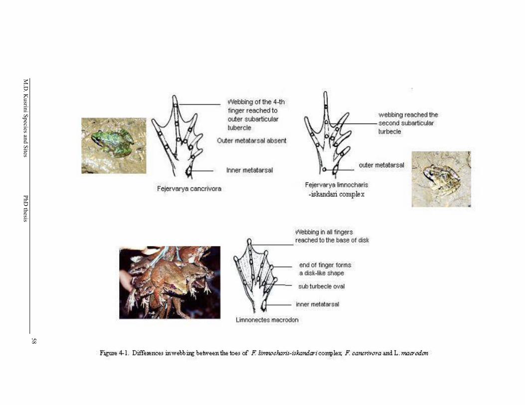
M.D
. Kusrini Species and Sites
PhD thesis
58
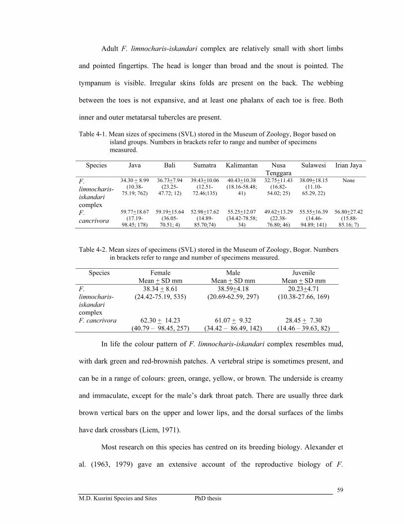
M.D. Kusrini Species and Sites PhD thesis
59
Adult F. limnocharis-iskandari complex are relatively small with short limbs
and pointed fingertips. The head is longer than broad and the snout is pointed. The
tympanum is visible. Irregular skins folds are present on the back. The webbing
between the toes is not expansive, and at least one phalanx of each toe is free. Both
inner and outer metatarsal tubercles are present.
Table 4-1. Mean sizes of specimens (SVL) stored in the Museum of Zoology, Bogor based on island groups. Numbers in brackets refer to range and number of specimens measured.
Species Java Bali Sumatra Kalimantan Nusa
Tenggara Sulawesi Irian Jaya
F. limnocharis-iskandari complex
34.30 + 8.99 (10.38-
75.19; 762)
36.73+7.94 (23.25-
47.72; 12)
39.43+10.06 (12.51-
72.46;135)
40.43+10.38 (18.16-58.48;
41)
32.75+11.43 (16.82-
54.02; 25)
38.09+18.15 (11.10-
65.29, 22)
None
F. cancrivora
59.77+18.67 (17.19-
98.45; 178)
59.19+15.64 (36.05-
70.51; 4)
52.98+17.62 (14.89-
85.70;74)
55.25+12.07 (34.42-78.58;
34)
49.62+13.29 (22.38-
76.80; 46)
55.55+16.39 (14.46-
94.89; 141)
56.80+27.42 (15.88-85.16; 7)
Table 4-2. Mean sizes of specimens (SVL) stored in the Museum of Zoology, Bogor. Numbers in brackets refer to range and number of specimens measured.
Species Female
Mean + SD mm Male
Mean + SD mm Juvenile
Mean + SD mm F. limnocharis-iskandari complex
38.34 + 8.61 (24.42-75.19, 535)
38.59+4.18 (20.69-62.59, 297)
20.23+4.71 (10.38-27.66, 169)
F. cancrivora 62.30 + 14.23 (40.79 – 98.45, 257)
61.07 + 9.32 (34.42 – 86.49, 142)
28.45 + 7.30 (14.46 – 39.63, 82)
In life the colour pattern of F. limnocharis-iskandari complex resembles mud,
with dark green and red-brownish patches. A vertebral stripe is sometimes present, and
can be in a range of colours: green, orange, yellow, or brown. The underside is creamy
and immaculate, except for the male’s dark throat patch. There are usually three dark
brown vertical bars on the upper and lower lips, and the dorsal surfaces of the limbs
have dark crossbars (Liem, 1971).
Most research on this species has centred on its breeding biology. Alexander et
al. (1963, 1979) gave an extensive account of the reproductive biology of F.

M.D. Kusrini Species and Sites PhD thesis
60
limnocharis found in Taiwan, including information on sex ratios, body size and age
distributions, growth rates, and reproductive biology. Jaafar (1994) observed the
reproductive ecology of this species in Malaysia, while Premo (1985) presented the only
study on the reproductive biology of this species in West Java. Fejervarya limnocharis
reproduces throughout the year (Alexander et al., 1963; Berry, 1964; Alexander et al.,
1979; Premo, 1985; Jaafar, et al., 1999) although in Taiwan the proportion of females
in reproductive condition peaks during spring (Alexander et al, 1979). Jaafar (1994)
found that the reproductive pattern of this species in paddy fields in Malaysia is
correlated with water levels.
Wide ranges of clutch sizes of F. limnocharis have been reported. Premo (1985)
reported that the average clutch size of West Java F. limnocharis was 1750, while Jaafar
et al. (1999) reported that the average clutch for Malayan F. limnocharis was 405.5 eggs
(sd = + 92.45, range 233 - 657). Genetic variation among East Asian populations of F.
limnocharis is thoroughly reviewed by Toda (1999).
Only two works have examined populations of F. limnocharis in rice fields.
Dash et al., (1993) gave the average density of F. limnocharis in irrigated paddy fields
in India as 39.12 frogs/ha, while Jaafar (1994) found adult densities ranging from 6.2 to
14.0 frogs/ha.
Fejervarya limnocharis is common in habitats associated with humans, such as
paddy fields and ponds (Berry, 1975; Premo, 1985; Iskandar, 1998). It is often
sympatric with F. cancrivora (Berry, 1964; Liem, 1971, Berry, 1975; Premo, 1985,
Jaafar, 1994; Iskandar, 1998).

M.D
. Kusrini Species and Sites
PhD thesis
61
M.D. Kusrini Species and Sites PhD thesis
62
My survey also found these frogs in streams near paddy field areas, as was also
recorded for MZB specimens. My surveys in West Java showed that F. limnocharis-
iskandari complex were in high abundance at both low and high elevations. At lower
elevations (less than 400 m asl) the abundance of this species is similar to that of F.
cancrivora, however, at upper elevations this species (or the new species mentioned
above) dominates the rice fields.
Iskandar mentioned that F. limnocharis is mostly found in lowlands and rarely
found more than 700 m above sea level (asl), except in areas where rice fields occur. I
found the species at higher elevations; up to 900 m asl (Cikaniki village, July 2004).
Similarly high elevations were noted for specimens in the collection of the MZB, as
noted by Alexander et al. (1979), who mentioned that the species can be found up to
1000 m asl.
4.2.2 The crab eating frog, Fejervarya cancrivora
Fejervarya cancrivora is a sturdy and large frog commonly found in rice fields.
Females are larger than males; mature males can be distinguished by the presence of
vocal sacs and black patches at the corner of the throat, and nuptial pads on their first
fingers. Fejervarya cancrivora was also known as Limnonectes cancrivorous or Rana
cancrivora Gravenhorst, 1829. Its common name is “crab-eating frog”, because its diet
includes large numbers of crabs. The species differs from F. limnocharis-iskandari
complex by its more extensive webbing between the toes and the absence of the outer
metatarsal tubercle. The colour in life is muddy brown or grey, with dark green or
brown patches in its skin. It has irregular longitudinal skin folds on its back. As with
F. limnocharis-iskandari complex, a dorsolateral stripe is sometimes present.

M.D
. Kusrini Species and Sites
PhD thesis
63
M.D. Kusrini Species and Sites PhD thesis
64
Church (1960) and Premo (1985) gave detailed accounts of F. cancrivora
breeding ecology in western Java, based on weekly examinations of frogs captured by
professional harvesters. Church (1960) noted that the species is shy and always ready to
jump when approached by humans. Apparently breeding is nearly aseasonal, and eggs
can be found at any time of the year, but according to Church (1960), the breeding
peaks from August through October.
There are conflicting reports regarding the clutch size of this species. Iskandar
(1998) and Jaafer et al. (1999) reported that clutches contain from 500 to more than
1000 eggs. In contrast, Premo (1985) stated that F. cancrivora clutches could contain
more than 10,000 eggs. Spawning can occur in two or even three batches and may tend
to peak during the dark phase of the moon (Church, 1960).
Although F. cancrivora is considered common, there are anecdotal accounts
suggesting that this species has disappeared from some rice field habitats in which it
was formerly abundant (e.g. Pratomo, 1998; Schmuck, 2000; Veith et al., 2001). There
is only one detailed population study on this species, carried out in Malaysia by Jaafar
(1994). Schmuck (2000) placed F. cancrivora on “at risk” status without actual data,
most probably because of its importance for human consumption.
Although it is most often encountered in rice fields, F. cancrivora is also found
in streams, ponds, ditches, and swamps in non-forested areas, mostly in habitats
associated with humans (Church; 1960; Alcala, 1962; Berry, 1975; Iskandar, 1998).
Both adult and larval F. cancrivora can be found in brackish water (Alcala, 1962;
Dunson, 1977). An experiment by Dunson (1977) revealed that tadpoles of this species
could survive high temperatures and salinities. Field notes accompanying specimens
stored at the MZB confirm that this species was mostly found in rice fields, although a
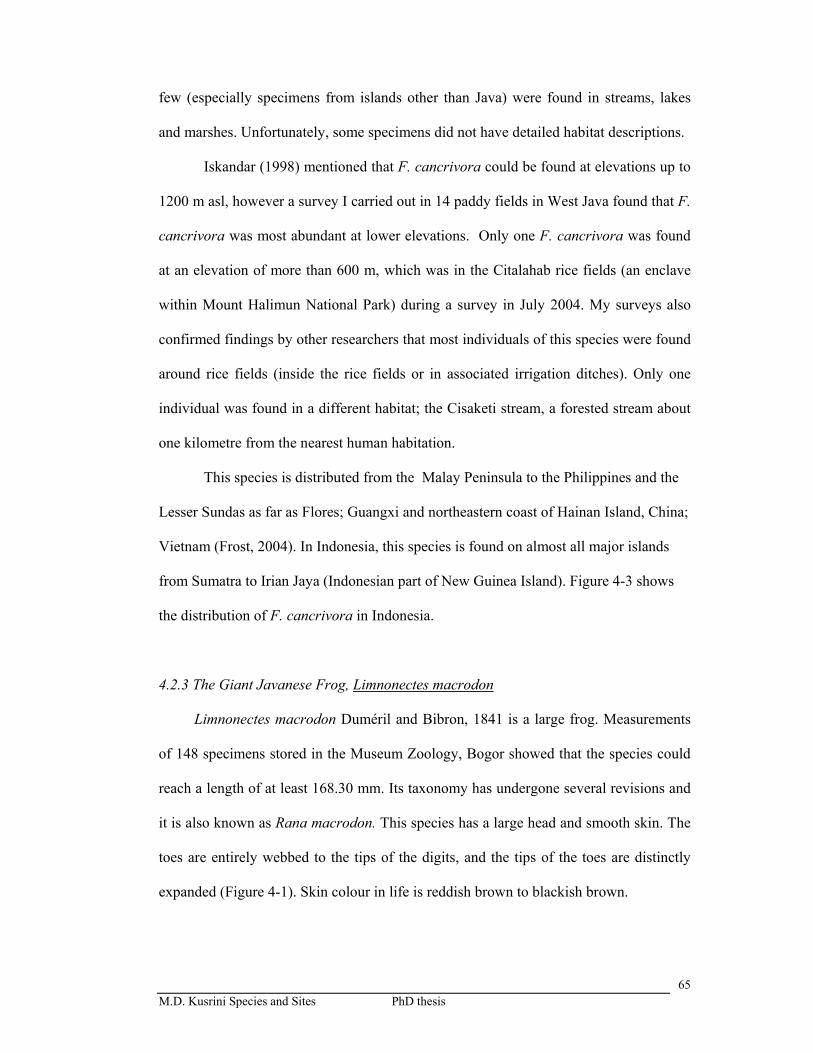
M.D. Kusrini Species and Sites PhD thesis
65
few (especially specimens from islands other than Java) were found in streams, lakes
and marshes. Unfortunately, some specimens did not have detailed habitat descriptions.
Iskandar (1998) mentioned that F. cancrivora could be found at elevations up to
1200 m asl, however a survey I carried out in 14 paddy fields in West Java found that F.
cancrivora was most abundant at lower elevations. Only one F. cancrivora was found
at an elevation of more than 600 m, which was in the Citalahab rice fields (an enclave
within Mount Halimun National Park) during a survey in July 2004. My surveys also
confirmed findings by other researchers that most individuals of this species were found
around rice fields (inside the rice fields or in associated irrigation ditches). Only one
individual was found in a different habitat; the Cisaketi stream, a forested stream about
one kilometre from the nearest human habitation.
This species is distributed from the Malay Peninsula to the Philippines and the
Lesser Sundas as far as Flores; Guangxi and northeastern coast of Hainan Island, China;
Vietnam (Frost, 2004). In Indonesia, this species is found on almost all major islands
from Sumatra to Irian Jaya (Indonesian part of New Guinea Island). Figure 4-3 shows
the distribution of F. cancrivora in Indonesia.
4.2.3 The Giant Javanese Frog, Limnonectes macrodon
Limnonectes macrodon Duméril and Bibron, 1841 is a large frog. Measurements
of 148 specimens stored in the Museum Zoology, Bogor showed that the species could
reach a length of at least 168.30 mm. Its taxonomy has undergone several revisions and
it is also known as Rana macrodon. This species has a large head and smooth skin. The
toes are entirely webbed to the tips of the digits, and the tips of the toes are distinctly
expanded (Figure 4-1). Skin colour in life is reddish brown to blackish brown.
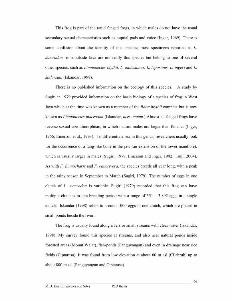
M.D. Kusrini Species and Sites PhD thesis
66
This frog is part of the ranid fanged frogs, in which males do not have the usual
secondary sexual characteristics such as nuptial pads and voice (Inger, 1969). There is
some confusion about the identity of this species; most specimens reported as L.
macrodon from outside Java are not really this species but belong to one of several
other species, such as Limnonectes blythii, L. malesianus, L. leporinus, L. ingeri and L.
kadarsani (Iskandar, 1998).
There is no published information on the ecology of this species. A study by
Sugiri in 1979 provided information on the basic biology of a species of frog in West
Java which at the time was known as a member of the Rana blythii complex but is now
known as Limnonectes macrodon (Iskandar, pers. comm.) Almost all fanged frogs have
reverse sexual size dimorphism, in which mature males are larger than females (Inger,
1966; Emerson et al., 1993). To differentiate sex in this genus, researchers usually look
for the occurrence of a fang-like bone in the jaw (an extension of the lower mandible),
which is usually larger in males (Sugiri, 1979, Emerson and Inger, 1992; Tsuji, 2004).
As with F. limnocharis and F. cancrivora, the species breeds all year long, with a peak
in the rainy season in September to March (Sugiri, 1979). The number of eggs in one
clutch of L. macrodon is variable. Sugiri (1979) recorded that this frog can have
multiple clutches in one breeding period with a range of 551 – 3,892 eggs in a single
clutch. Iskandar (1998) refers to around 1000 eggs in one clutch, which are placed in
small ponds beside the river.
The frog is usually found along rivers or small streams with clear water (Iskandar,
1998). My survey found this species at streams, and also near natural ponds inside
forested areas (Mount Walat), fish-ponds (Panguyangan) and even in drainage near rice
fields (Ciptarasa). It was found from low elevation at about 60 m asl (Cilabruk) up to
about 800 m asl (Panguyangan and Ciptarasa).
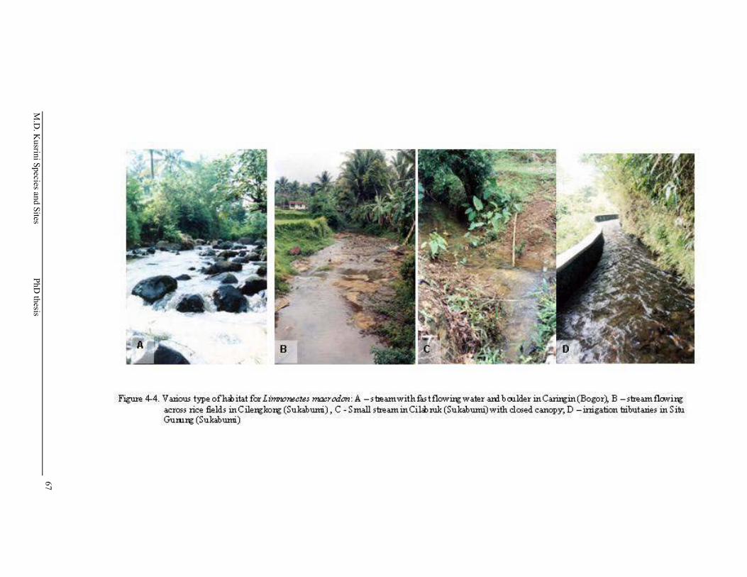
M.D
. Kusrini Species and Sites
PhD thesis
67
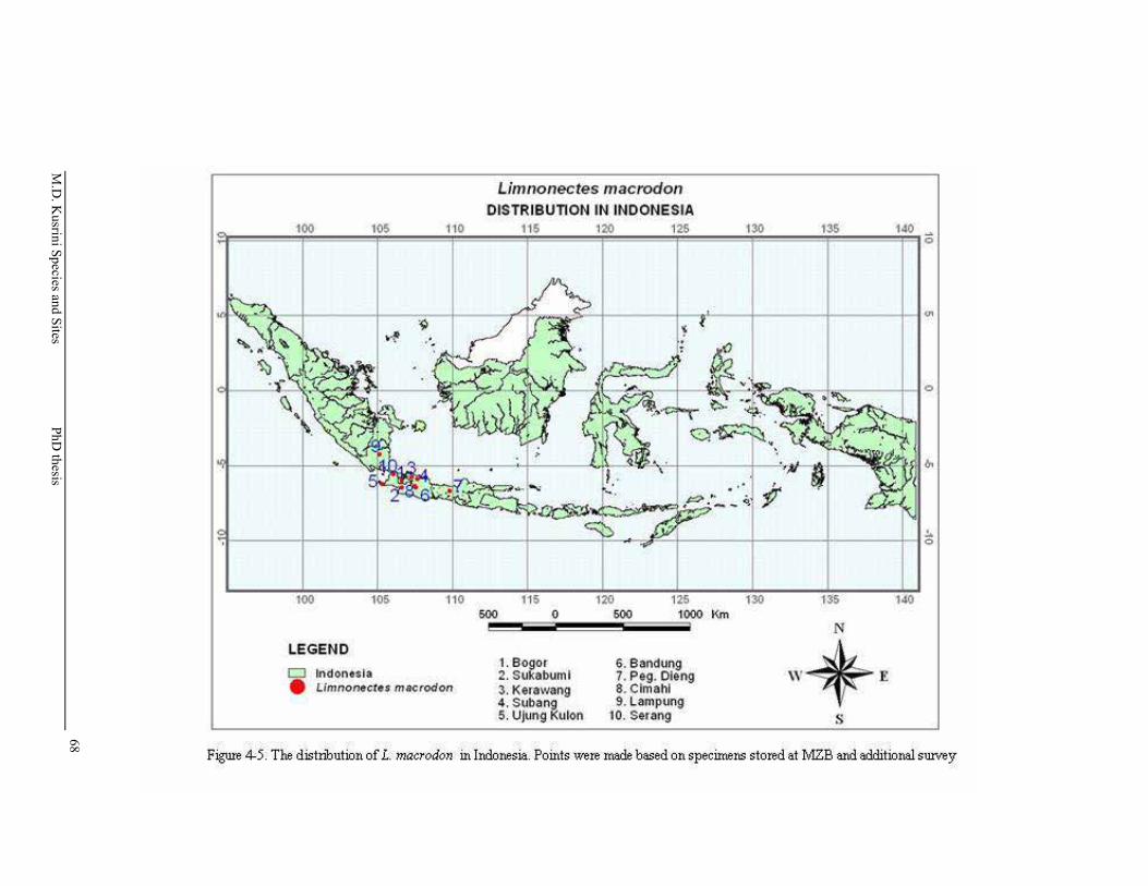
M.D
. Kusrini Species and Sites
PhD thesis
68
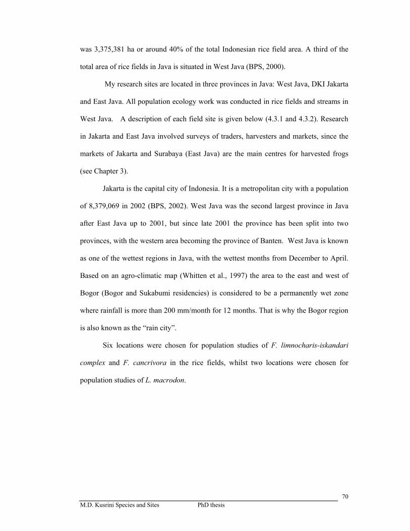
M.D. Kusrini Species and Sites PhD thesis
70
was 3,375,381 ha or around 40% of the total Indonesian rice field area. A third of the
total area of rice fields in Java is situated in West Java (BPS, 2000).
My research sites are located in three provinces in Java: West Java, DKI Jakarta
and East Java. All population ecology work was conducted in rice fields and streams in
West Java. A description of each field site is given below (4.3.1 and 4.3.2). Research
in Jakarta and East Java involved surveys of traders, harvesters and markets, since the
markets of Jakarta and Surabaya (East Java) are the main centres for harvested frogs
(see Chapter 3).
Jakarta is the capital city of Indonesia. It is a metropolitan city with a population
of 8,379,069 in 2002 (BPS, 2002). West Java was the second largest province in Java
after East Java up to 2001, but since late 2001 the province has been split into two
provinces, with the western area becoming the province of Banten. West Java is known
as one of the wettest regions in Java, with the wettest months from December to April.
Based on an agro-climatic map (Whitten et al., 1997) the area to the east and west of
Bogor (Bogor and Sukabumi residencies) is considered to be a permanently wet zone
where rainfall is more than 200 mm/month for 12 months. That is why the Bogor region
is also known as the “rain city”.
Six locations were chosen for population studies of F. limnocharis-iskandari
complex and F. cancrivora in the rice fields, whilst two locations were chosen for
population studies of L. macrodon.

M.D. Kusrini Species and Sites PhD thesis
71
4.3.1 Rice fields
a. Locations
Intensive studies of the population dynamics of F. limnocharis-iskandari
complex and F. cancrivora and of pesticide residues were conducted in six rice fields in
the Kabupaten (Residencies) of Bogor, Karawang and Subang, from May 2002 until
October 2003.
Two locations were sampled in the Bogor area; Caringin and Darmaga village.
The sawah or rice fields in this area are small and situated between home-gardens
(kebun) and villages. The area sampled in Darmaga was a research plot owned by the
nearby Bogor Agricultural University. The Caringin and the Darmaga rice fields are
subject to high annual rainfall. During my study, the wettest month occurred in
February 2003 (571 mm in Caringin and 556 mm in Darmaga) and the driest month in
July 2003 (43 mm in Caringin and 25 mm in Darmaga). Figure 4-6 shows the monthly
rainfall during 2002 and 2003.
Karawang and Subang are situated in the northern coastal lowland part of West
Java, with less annual rainfall than Bogor and Sukabumi, and have distinct dry seasons.
The countryside is flat, most trees are concentrated within the villages, and rice fields
dominate the terrain. The rice fields sampled in Karawang were located at the village of
Cikuntul, whilst in Subang they were located at the village of Sukahaji (around 40 km
east of Cikuntul).
Samples were taken from four rice fields in these areas:, two in Karawang and
two in Subang. In each area I sampled one pesticide rice field (code P) and one non-
pesticide rice field (code NP). The fields sampled were situated in huge arrays of sawah
and the distances between the pesticide and non-pesticide locations were approximately
500 m and 2000 m for Karawang and Subang respectively.
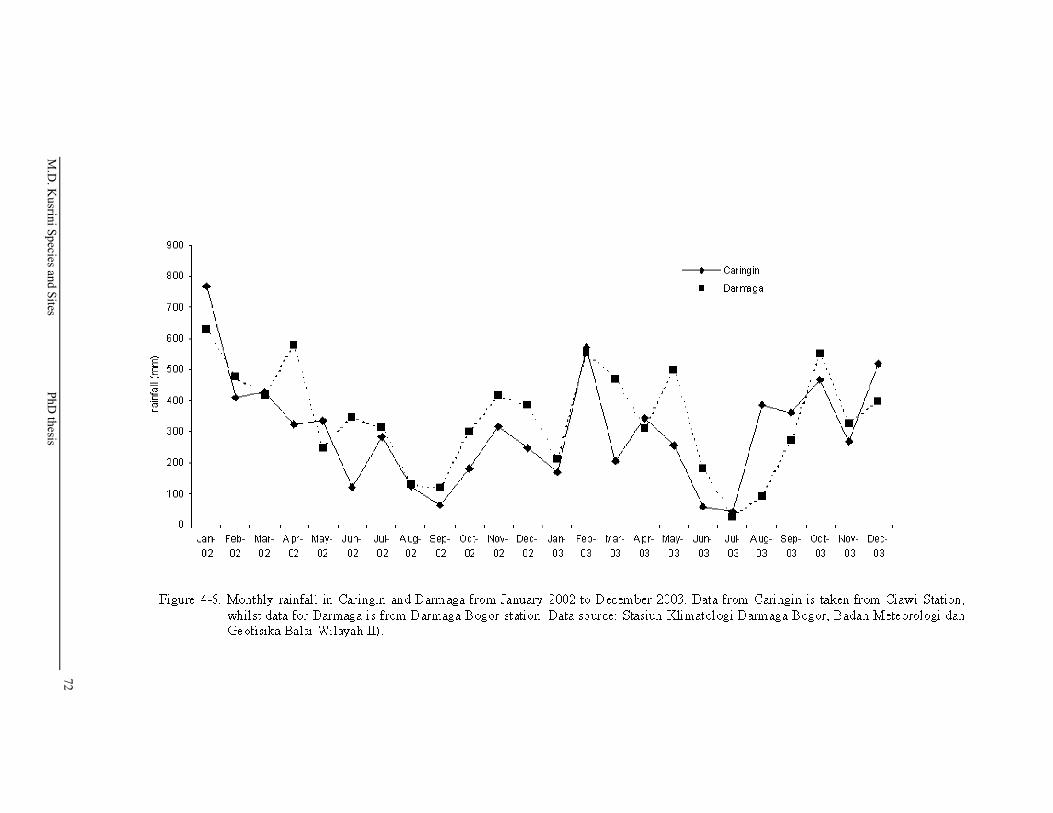
M.D
. Kusrini Species and Sites
PhD thesis
72

M.D
. Kusrini Species and Sites
PhD thesis
73

M.D. Kusrini Species and Sites PhD thesis
74
The non-pesticide rice fields in Karawang were owned by a single farmer who
has not used pesticide since 1990. The non-pesticide rice fields in Subang were owned
by a group of farmers who decided to turn to integrated pest management in 2000. Thus
the total area of non-pesticide rice fields in Subang is 10 times bigger than the total area
of non-pesticide rice fields in Karawang. The relatively short times since pesticide use
ceased means that residual pesticides might still be present, particularly the more
persistent types such as organochlorines. Unfortunately, there were no fields with less
likelihood of pesticide residues available for sampling.
Figure 4-7 shows the monthly rainfall in the area during 2002 and 2003.
Throughout the whole period of sampling (May 2002 to September 2003), the
meteorological bureau offices in Karawang and Subang area recorded no rain. 2003
was a dry year compared to 2002, with total annual rainfall of 257 mm compared with
1227 mm in 2002. Table 4-4 shows air and water temperatures and relative humidity at
the six sites during the study.
Surveys to check the occurrence of the target species were also undertaken in
eight other locations: Situ Gede (Bogor), Cisaat (the buffer zone of Mount Gede-
Pangrango National Park), Panguyangan and Ciptarasa (both enclaves within Mount
Halimun National Park), Citalahab (also an enclave in Mount Halimun NP), Ciracap
and Lengkong. Figure 4-8 shows the location of rice field surveys.
The first four locations were surveyed during August-September 2001,
Citalahab was surveyed in July 2004, and the last two during October 2003. In March
2004, Situ Gede rice fields were used for a 6-days movement study of F. cancrivora
(Chapter 5). Full descriptions and locations of these sites appear in Table 4.5.

M.D. Kusrini Species and Sites PhD thesis
75
Table 4-4. Microclimate in the paddy fields of Bogor, Karawang and Subang. Data were recorded at 21.00 – 24.00 hours.
Location Microclimate
Range Mean + SD
Caringin Air temp (oC) 20.0 - 23.5 21.3 + 1.0 Water temp (oC) 21.0 - 24.5 23.1 + 1.1 Relative Humidity (%)
84 - 96 90.6 + 4.1
Darmaga Air temp (oC) 21.8 - 26.2 23.7 + 1.3 Water temp (oC) 24.2 - 26.0 25.2 + 0.9 Relative Humidity (%)
85 - 97 94.1 + 3.6
Karawang NP Air temp (oC) 22.4 - 27.4 24.9 + 1.5 Water temp (oC) 24.9 - 28.1 26.3 + 1.3 Relative Humidity (%)
86 - 96 92.1 + 3.7
Karawang P Air temp (oC) 22.4 - 27.4 25.0 + 1.5 Water temp (oC) 24.9 - 28.1 26.3 + 1.2 Relative Humidity (%)
86 - 96 92.4 + 3.9
Subang NP Air temp (oC) 22.0 - 26.0 23.7 + 1.5 Water temp (oC) 23.2 - 27.0 25.1 + 1.4 Relative Humidity (%)
81 - 98 93.9 + 5.0
Subang P Air temp (oC) 22.0 - 26.0 23.8 + 1.4 Water temp (oC) 24.0 - 27.0 25.3 + 1.6 Relative Humidity (%)
81 - 99 93.0 + 4.2
Five sawah were surveyed in Sukabumi. Except for Ciracap, which was situated
in low land, the others were situated in the sloping terrain within an enclave of a
National Park (Ciptarasa and Panguyangan, Citalahab, all village enclaves inside Mt.
Halimun National Park) or on the border of a National Park (Cisaat and Situ Gunung,
bordering Mt. Gede-Pangrango National Park). Although focusing more on the
occurrence of F. limnocharis-iskandari complex and F. cancrivora, I also noted other
species present. Figure 4-8 shows the locations of rice fields surveyed during the study.
M.D
. Kusrini Species and Sites
PhD thesis
76

M.D. Kusrini Species and Sites PhD thesis
77
b. Rice planting methods and management
Rice growing in Indonesia is mostly done using wet-field cultivation, in which
rice grows in water and is dependent on rainwater run-off or artificial irrigation (van
Setten van den Meer, 1979). Rice fields or sawah are an important agriculture
landscape in Indonesia. They are the main source of Indonesia’s staple food, and are
also an important habitat for wildlife, including fish, birds and frogs (Whitten, et. al.
1997). Edible frogs, such as Fejervarya limnocharis-iskandari complex and F.
cancrivora, occur abundantly in rice fields (Chapter 5), thus the habitat is important in
sustaining the edible frog trade.
Rice, Oryza sativa, is planted either in flat areas or in terrace systems in upland
areas. Land is usually separated into blocks of sawah, divided by small borders and
flooded just before sowing. The borders serve both as property boundaries and as water
regulation systems. Preparation begins with the farmer raking and ploughing the rice
field with water buffaloes when water fills the field. Rice seeds are planted in small
plots, germination takes place 7–15 days later, and rice plants emerge from the water
approximately 30 days after sowing. Seedlings are separated and planted in the rice
fields. Once seedlings are rooted, water levels (20–30 cm) are periodically reduced (5–
10 cm) several times during the season for herbicide and pesticide spraying or
fertilization. Rice fields are drained some days before harvesting. Rice is harvested
about four months after planting. In intensive areas like Subang and Karawang, the
fallow period is short and fields are prepared as soon as possible for another growing
season. In other areas, usually those dependent on water from run-off, farmers
sometimes grow cash crops such as beans or other vegetables intermittently with the
rice-planting season or leave the fields to “wild” aquatic plants. Figure 4-9 shows
various stage of rice planting.
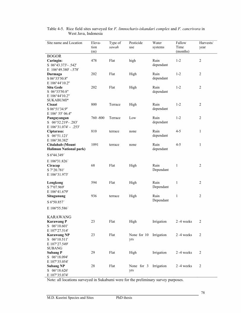
M.D. Kusrini Species and Sites PhD thesis
78
Table 4-5. Rice field sites surveyed for F. limnocharis-iskandari complex and F. cancrivora in West Java, Indonesia
Site name and Location Eleva-
tion (m)
Type of sawah
Pesticide use
Water systems
Fallow Time (months)
Harvests/ year
BOGOR Caringin: S 06°43.373′- .542′ E 106°49.380′ -.578′
478 Flat high Rain dependant
1-2 2
Darmaga S 06°33′50.8″ E 106°44′10.2″
202 Flat High Rain dependant
1-2 2
Situ Gede S 06°33'50.8" E 106°44'10.2"
202 Flat High Rain dependant
1-2 2
SUKABUMI* Cisaat S 06°51′34.9″ E 106° 55′ 06.4″
800 Terrace High Rain dependant
1-2 2
Panguyangan S 06°52.219′- .283′ E 106°31.074′ - .253′
760 -800 Terrace Low Rain dependant
1-2 2
Ciptarasa: S 06°51.121′ E 106°30.382′
810 terrace none Rain dependant
4-5 1
Citalahab (Mount Halimun National park) S 6º44.349´
E 106º31.826´
1091 terrace none Rain dependant
4-5 1
Ciracap S 7°20.781′ E 106°31.973′
68 Flat
High
Rain Dependant
1
2
Lengkong S 7°07.969′ E 106°41.679′
594 Flat High Rain Dependant
1 2
Situgunung
S 6º50.857´
E 106º55.586´
936 terrace High Rain Dependant
1 2
KARAWANG Karawang P S 06°10.601′ E 107°27.514′
23 Flat High Irrigation 2 -4 weeks 2
Karawang NP S 06°10.511′ E 107°27.549′
23 Flat None for 10 yrs
Irrigation 2 -4 weeks 2
SUBANG Subang P S 06°18.094′ E 107°35.054′
29 Flat High Irrigation 2 -4 weeks 2
Subang NP S 06°18.626′ E 107°35.074′
28 Flat None for 3 yrs
Irrigation 2 -4 weeks 2
Note: all locations surveyed in Sukabumi were for the preliminary survey purposes.
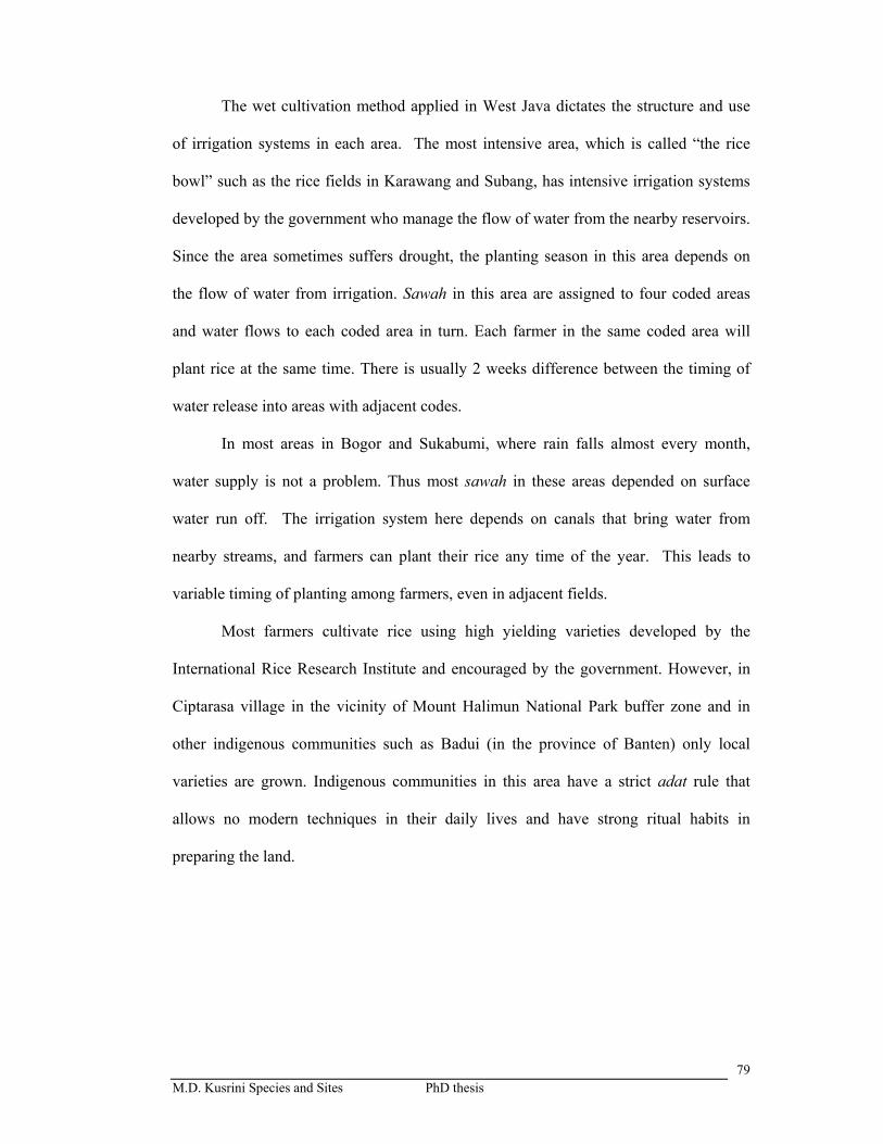
M.D. Kusrini Species and Sites PhD thesis
79
The wet cultivation method applied in West Java dictates the structure and use
of irrigation systems in each area. The most intensive area, which is called “the rice
bowl” such as the rice fields in Karawang and Subang, has intensive irrigation systems
developed by the government who manage the flow of water from the nearby reservoirs.
Since the area sometimes suffers drought, the planting season in this area depends on
the flow of water from irrigation. Sawah in this area are assigned to four coded areas
and water flows to each coded area in turn. Each farmer in the same coded area will
plant rice at the same time. There is usually 2 weeks difference between the timing of
water release into areas with adjacent codes.
In most areas in Bogor and Sukabumi, where rain falls almost every month,
water supply is not a problem. Thus most sawah in these areas depended on surface
water run off. The irrigation system here depends on canals that bring water from
nearby streams, and farmers can plant their rice any time of the year. This leads to
variable timing of planting among farmers, even in adjacent fields.
Most farmers cultivate rice using high yielding varieties developed by the
International Rice Research Institute and encouraged by the government. However, in
Ciptarasa village in the vicinity of Mount Halimun National Park buffer zone and in
other indigenous communities such as Badui (in the province of Banten) only local
varieties are grown. Indigenous communities in this area have a strict adat rule that
allows no modern techniques in their daily lives and have strong ritual habits in
preparing the land.
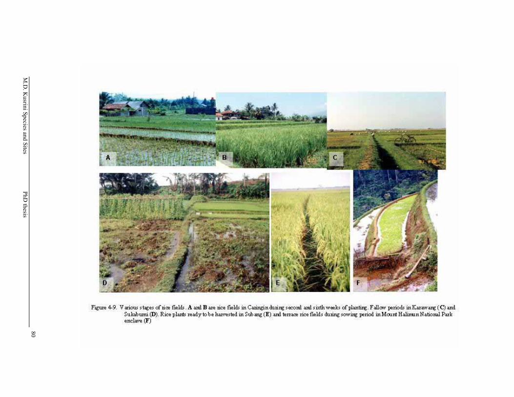
M.D
. Kusrini Species and Sites
PhD thesis
80

M.D. Kusrini Species and Sites PhD thesis
81
The need for greater rice productivity has resulted in higher levels of pesticide
and fertilizer input to rice fields (Settle, et al., 1996). Moreover, the development of
more efficient water irrigation systems has shifted rice planting methods from
traditional methods which use low input and fewer planting seasons in a year (one or
two times) into high input and more planting seasons in a year (2 or 3 times a year), thus
reducing the fallow times. Excess use of pesticide is known to affect the biodiversity of
rice field communities in Indonesia (Settle et al., 1996) and pesticides have been
implicated as one of the culprits in amphibian declines around the world (Ouelett, et al.,
1997; Taylor, et. al, 1999; Bridges and Semlitsch, 2000)
Sawah in Karawang and Subang are usually farmed intensively, with two
planting seasons yearly. Although, the government of Indonesia tries to encourage
lower use of pesticides, their use by Indonesian farmers is still high. Investigations by
Ardiwinata et al. (1997) into pesticide levels in samples of soil, water and rice collected
from West Javan areas including Karawang, Subang, and Sukabumi revealed high
levels of chlorpirifos, BHC, aldrin, endosulfan and carbofuran in the soil samples. The
high cost of pesticides and better understanding of pesticide risk has turned some
farmers to integrated pest management system (IPM), using no pesticides and relying on
biological pest control. The number of farmers using IPM in Subang and Karawang is
still small, and the total area of rice fields under IPM is relatively small. Most blocks of
sawah under IPM are situated in the middle of a huge array of pesticide-use rice fields
and therefore the benefit to them of using IPM is not really known. In contrast to these
systems, the indigenous communities in Mt. Halimun National Park area in Sukabumi
residency have maintained their traditional agricultural systems. The methods include a
long fallow period, low number of planting seasons per year and no use of pesticides. A
summary of sawah conditions in each location appears in Table 4-5.

M.D. Kusrini Species and Sites PhD thesis
82
4.3.2 Streams
The population dynamics of L. macrodon were studied in two locations:
Cilember and Ciapus Leutik, from June 2002 to May 2003. Both locations were near
forested land, although the location at Ciapus Leutik was nearer to human habitat, in
this case Ciapus village.
Additional surveys to find L. macrodon were conducted in eight other locations
in West Java. Three streams (Cinagara, Cikalang, and Mount Walat streams) were
surveyed twice during 2002-2003, and five locations were surveyed once (Cisaketi
Stream; Cilabruk Stream, Cilengkong Stream, tributaries around Situ Gunung lake and
Situ Gunung stream).
The streams and the lake surveyed differed in various characteristics. Some
were located near villages and sometimes crossed through rice fields (Caringin,
Cikalang, Mount Walat and Ciapus, Situ Gunung stream, Cilabruk and Cilengkong),
others were located in forested areas (Cisaketi and Situ Gunung Lake). Table 4-6 gives
the characteristics of the streams and full descriptions of study sites, whilst Figure 4-10
shows the locations of these surveys. Details of the results of the surveys conducted in
rice fields and streams appear in chapters 5, 6, and 7.
M.D. Kusrini Species and Sites PhD thesis
83
Table 4-6. Streams and ponds surveyed for L. macrodon.
Site name and Location Elevation (m)
Flow status Adjacent landscape
BOGOR
Cinagara – Caringin: S 06°43.373′- .542′ E 106°49.380′ -.578′
479 – 491 Permanent streams
Village and rice fields
Cikalang S 06°43.216′ E 106°49.775′
458 Permanent streams
Village and rice fields
Ciapus Leutik* S 06°39.800′ - .901′ E 106°44.711′ - .715′
709 - 717
Permanent streams
Village and Plantation forest
Cilember* S 06°39.612′ - .631′ E 106°56.701′ - 57.002′
662 – 840 m Permanent streams
Plantation Forest and Recreational area
SUKABUMI
Mount Walat S 06°54.879′ E 106°49.445′
595 Permanent streams
Village and rice fields
Cisaketi S 06°44.471′ - .559′ E 106°38.453′ - .882′
951 – 1039 Permanent streams
Forested area, inside Unocal Gas Mining
Cilabruk S 07°20.263′ - .423′ E 106°31.981′ - 32.169′ Cilengkong S 07°07.852′ - .967′ E 106°41.682′ - .725′
69 - 101 578 - 591
Permanent streams
Rice field Village and Rice fields and crops
Situ Gunung S 06°50.017′ - .077′ E 106°55.399′ - .417′
1045 Permanent streams
Plantation Forest and Recreational area, rice fields
Situ Gunung Lake S 6º50.239´ - .992’ E 106º55.564´ -.652’
921 – 1071 Permanent lake Plantation Forest and Recreational area, rice fields
* Population study sites. Other sites were preliminary survey

M.D
. Kusrini Species and Sites
PhD thesis
84

M.D. Kusrini Rice fields’ frog population PhD thesis
85
CHAPTER 5
POPULATION DYNAMICS OF F. LIMNOCHARIS-ISKANDARI COMPLEX
AND F. CANCRIVORA
5.1 Introduction
As a country, Indonesia relies heavily on its agricultural sector. Because rice is
the staple food for most of the nearly 200 million inhabitants of Indonesia, it is not
surprising that its agricultural land is predominantly paddy fields. Paddy fields are an
important habitat for wildlife such as birds, reptiles and amphibians (Whitten et al.,
1997) and some 3.5 million hectares of paddy fields are available as habitat for
amphibians in the island of Java alone. Compared with other habitats, the number of
frog species in agricultural land is usually low (Dash and Mahandata, 1998; Jaafar et al.,
2002), however species adapted to the conditions encountered in this system are usually
abundant. Some frogs, such as Fejervarya limnocharis and F. cancrivora, thrive in
paddy fields (Church, 1960; Alexander et al., 1963 and 1979, Jaafar, 1994) despite the
physiological stress that might occur because of human activity.
Although some studies on paddy field frog species have been done in Indonesia
(Church, 1960, Atmowidjojo and Boeadi, 1988; Premo, 1989), these studies have
usually focused on aspects of the biology of one species, such as clutch size, fecundity
and food habits, by analysing specimens obtained from professional harvesters. Thus
there is little detailed information on the population sizes and dynamics of the most
common frogs in Indonesian paddy fields: F. limnocharis-iskandari complex and F.
cancrivora. Both species are heavily exploited for human consumption (chapter 2 and
3) and to evaluate the sustainability of current harvesting practices there is a need to
have a clear understanding of the population dynamics of these species.
M.D. Kusrini Rice fields’ frog population PhD thesis
86
To estimate populations, a number of mathematical models have been
developed. To apply these models, parameters must be estimated, usually using data
collected from mark-release-recapture studies. Mark recapture techniques have been
widely used for estimating population size and other parameters such as mortality,
emigration rates, birth and immigration rates for a range of animal groups, such as frogs
(Friedl and Klump, 1997; Ramirez et al., 1998; Wood et al., 1998, Peters, 2001), lizards
(Bennett, 2000), dolphins (Baird et al., 2001), or insects (Zun’iga et al, 2001).
These techniques can be used for closed or open populations. For the purposes
of mark-recapture analysis, closed populations are those in which the effects of birth,
death, immigration, and emigration can be assumed to be zero during the periods over
which data are collected. Open populations are those that may be affected by these
processes during data collection (Krebs, 1999).
Populations of frogs are influenced by many factors, such as climatic conditions
(Lips, 1998), food availability (Lima et. al, 1995; Pope and Matthews, 2002),
competition and predation (BrÖnmark and Edenham, 1994; Gillespie, 2001) and
territoriality (Heying, 2001). The study area lies in West Java, which is a tropical region
with high annual rainfall, and the rice field habitat undergoes repeated harsh physical
conditions such as flooding and draining, depending on the stage of the harvest cycle
(see Chapter 4 for detailed account). In Malaysia, the reproductive pattern of F.
limnocharis and F. cancrivora in the paddy fields is correlated to the water regime in
the rice fields (Jaafar, 1994).
The dynamics of populations can be affected by patterns of individual
movements. Because environmental conditions in rice fields are dynamic, it is likely
that frogs move between them to avoid the harsher extremes. This leads to questions
such as: What becomes of animals when the habitat dries? Do they stay and aestivate or
M.D. Kusrini Rice fields’ frog population PhD thesis
87
do they move elsewhere? What are the frequency and extent of short-term movements,
and how will they affect mark-recapture population estimates? To date, no studies have
been conducted on detailed microhabitat use and movement patterns of rice field frogs.
In fact, there is little detailed information on movement patterns of most anurans
(Beebee, 1996). Animal movements are likely to be affected by the availability of
resources and avoidance of predators (Lemckert and Brassill, 2000; Schwarzkopf and
Alford 2002, Pough et al., 2004). F. limnocharis and F. cancrivora are widespread in
most of Asia (Frost, 1985) and are found mostly in agricultural land. Information on the
dynamics of these populations would give insight into the success of species that inhabit
rice fields.
This chapter presents the population biology of F limnocharis-iskandari
complex and F. cancrivora in several paddy fields in West Java, and includes the results
of a detailed study on individual movements of F. cancrivora.
5.2 Methods
5.2.1 Population study
Populations of both species were studied at six sites: Caringin, Darmaga, Subang
1 (Non Pesticide) and Subang 2 (Pesticide), Karawang 1 (Non Pesticide) and Karawang
2 (Pesticide) over four discrete times which included two planting seasons, one in 2002
and the other in 2003 (table 5-1). All rice field locations are harvested twice a year.
Chapter 4 gives detailed descriptions of each site. Field parties consisted of 4-6 persons
using battery-powered torches, who surveyed paddy fields between 20.00 hrs and 24.00
hrs. Frogs were collected manually.
In total, twelve days of sampling were carried out at each location, divided into
four periods. One plot in a paddy field at each site was sampled for three days in a row,
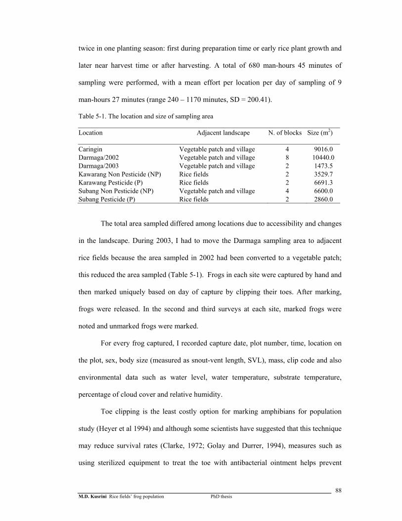
M.D. Kusrini Rice fields’ frog population PhD thesis
88
twice in one planting season: first during preparation time or early rice plant growth and
later near harvest time or after harvesting. A total of 680 man-hours 45 minutes of
sampling were performed, with a mean effort per location per day of sampling of 9
man-hours 27 minutes (range 240 – 1170 minutes, SD = 200.41).
Table 5-1. The location and size of sampling area Location Adjacent landscape
N. of blocks Size (m2)
Caringin Vegetable patch and village 4 9016.0 Darmaga/2002 Vegetable patch and village 8 10440.0 Darmaga/2003 Vegetable patch and village 2 1473.5 Kawarang Non Pesticide (NP) Rice fields 2 3529.7 Karawang Pesticide (P) Rice fields 2 6691.3 Subang Non Pesticide (NP) Vegetable patch and village 4 6600.0 Subang Pesticide (P) Rice fields 2 2860.0
The total area sampled differed among locations due to accessibility and changes
in the landscape. During 2003, I had to move the Darmaga sampling area to adjacent
rice fields because the area sampled in 2002 had been converted to a vegetable patch;
this reduced the area sampled (Table 5-1). Frogs in each site were captured by hand and
then marked uniquely based on day of capture by clipping their toes. After marking,
frogs were released. In the second and third surveys at each site, marked frogs were
noted and unmarked frogs were marked.
For every frog captured, I recorded capture date, plot number, time, location on
the plot, sex, body size (measured as snout-vent length, SVL), mass, clip code and also
environmental data such as water level, water temperature, substrate temperature,
percentage of cloud cover and relative humidity.
Toe clipping is the least costly option for marking amphibians for population
study (Heyer et al 1994) and although some scientists have suggested that this technique
may reduce survival rates (Clarke, 1972; Golay and Durrer, 1994), measures such as
using sterilized equipment to treat the toe with antibacterial ointment helps prevent

M.D. Kusrini Rice fields’ frog population PhD thesis
89
infection that could lead to mortality (Reaser and Dexter, 1996). A recent study found
that the adverse impact of toe clipping could increase with the number of toes removed
(McCarthy and Parris, 2004). To minimize the impact of toe clipping, I only clipped one
to two toes of each individual captured. When two toes were removed, I clipped one
from a forelimb and one from a hindlimb. I also avoided clipping the first digit on the
forefeet (the “thumb”) because of its potential role in amplexus in males.
5.2.2 Determination of sex
The sexes of F. limnocharis-iskandari complex and F. cancrivora were
differentiated based on secondary sexual characteristics. Fejervarya limnocharis-
iskandari complex males have pigmentation on their throats, which in adults is
distinctly M shaped, whilst in juveniles only a faint trace is visible. Males also have a
pair of vocal sacs and during breeding possess nuptial pads. Male F. cancrivora also
have a black patch on their throats, although this is not as large as in F. limnocharis-
iskandari complex.
The smallest frogs exhibiting the black patch and vocal sacs were 17.46 mm in
SVL weighing 0.6 gram (F. limnocharis-iskandari complex) and 25.0 mm in SVL
weighing 1.15 gram (F. cancrivora). However, only frogs judged to be mature based on
body size (based on research by Church (1960), Alexander (1978), Premo (1989), and
Jaafar (1994)) were assigned to adult sex categories. Therefore, F. limnocharis-
iskandari complex designated as males were frogs who exhibited secondary sexual
characteristics and were 25 mm or more in length, and females of this species were
frogs lacking male secondary sex characteristics and with lengths of 30 mm or more. F.
cancrivora were assigned similarly, with minimum lengths of 35mm for males and

M.D. Kusrini Rice fields’ frog population PhD thesis
90
40mm for females. Individuals with lengths below the cutoffs for their species were
classified as juveniles.
5.2.3 Skeletochronology
Selected phalanges taken from toe clips of F. limnocharis-iskandari complex
and F. cancrivora were examined to determine age using skeletochronology.
Skeletochronology has been used successfully to estimate age in temperate frogs
(Halliday and Verrel, 1988; Ryser, 1988; Reaser, 2000). In this study skeletochronology
was carried out on 103 F. limnocharis-iskandari complex and 35 F. cancrivora from
samples taken in preliminary surveys during 2001 in several paddy fields in West Java
at Caringin, Darmaga, Ciptarasa, Panguyanan and Ciptarasa.
Clipped toes removed from frogs during surveys were stored in 4% formalin
solution for processing. Each toe was wrapped in sponge and placed individually in a
cassette, then decalcified overnight in 10% formic acid solution. Toes were then
embedded in wax in a vacuum infiltration processor and cut into 10µm thick sections
transversely using a rotary microtome. Sections were put on slides and kept in a
warming oven at least overnight. They were then placed into two consecutive baths of
xylene for two minutes each, and then placed into three consecutive baths of ethanol for
20 dips each before being rinsed in water and stained with Mayer’s Haematoxylin and
Young’s Eosin for 25 minutes. Slides were then rinsed again in water and put into
Scott’s tap water substitute for two minutes. After a final rinse in water, the slides were
put in Young’s Eosin stain for five dips and then exposed to a series of 10 dips in
ethanol and a final 10 dips in xylene. Cover slips were then mounted with DPX glue and
slides were placed on trays in a 60oC oven overnight. The best and clearest sections
M.D. Kusrini Rice fields’ frog population PhD thesis
91
were chosen for observations and were examined using an Olympus BH dual-head
microscope to view marks of skeletal growth.
5.2.4 Sampling bias
To check for sampling bias in paddy field surveys (since frogs were caught
mostly when they were 0.5 m or less from the field’s perimeter), on at least one
occasion at each site, frogs were sampled simultaneously not only from within 50 cm of
the perimeter but also inside the plot. To avoid damage to rice plants, this sampling was
done after harvesting. Frogs were treated the same as in the first sampling, by marking
and releasing them afterward for three consecutive nights. In calculating densities, the
sampled area was assumed to be 150 cm wide, except at Darmaga, which was assumed
to be 100 cm wide. The width of the border in Darmaga is narrower than other locations
(maximum width 15 cm, compared to other locations with maximum width 50 cm).
These perimeter widths include the width of pathways that act as borders separating
blocks of rice fields.
5.2.5 Movement of F. cancrivora
Additional sampling to assess population densities and movements of F.
cancrivora was conducted in Darmaga during March 2004. The sampled paddy field
had been harvested and half of the blocks in it had been prepared for tilling. Heavy rain
occurred during the sampling period and most of the areas were temporarily flooded
with water; this flooding usually subsided after a few hours. The new site was
approximately 2 km from the site used in the original population study. A party of 11-
13 persons surveyed 4,592.83 m2 of paddy fields (composed of nine blocks) for six days
in a row with total effort of 274 man-hours 45 minutes or mean daily effort of 45 man-

M.D. Kusrini Rice fields’ frog population PhD thesis
92
hours 47 minutes and 30 seconds. Since sampling was focused on the occurrence of F.
cancrivora other frogs were only noted and released immediately. Each F. cancrivora
captured was assigned a unique code by clipping its toes based on Hero’s (1989)
numbering system but omitting codes requiring clipping the “thumb”. The snout-vent
length and mass of each frog were measured before its release at its point of capture. A
flag with the individual’s ID number was put at each location where a frog was
captured. A path on one side and an irrigation channel perpendicular to the path
bordered the blocks of rice fields; we used these as X and Y axes in mapping the
positions of frogs. When frogs were recaptured, we noted their position only and
released them at the point of capture.
5.3. Data analysis
All data sets were analysed using Microsoft Excel and SPSS (version 12.0.1,
2003). The mass and snout vent length of both species were analysed using descriptive
statistics. Mean SVLs of males and females within sites were compared using
independent samples t-tests for equal variance. Correlation analyses between log-
transformed mass and log-transformed snout vent length were undertaken on both
species.
The relationship between SVL and number of lines of arrested growth (LAG)
was examined for both species using simple scatter graphs and by analyzing the
differences of mean SVL between groups that had LAGs and no LAGs. Size-frequency
histograms were produced for both sexes of both species at each of the six study sites
for each discrete sampling time. Data on snout-vent length were pooled into 1 cm size
class categories. I used log-linear analysis to examine relationships between three
categorical variables: size class, location and sampling time.
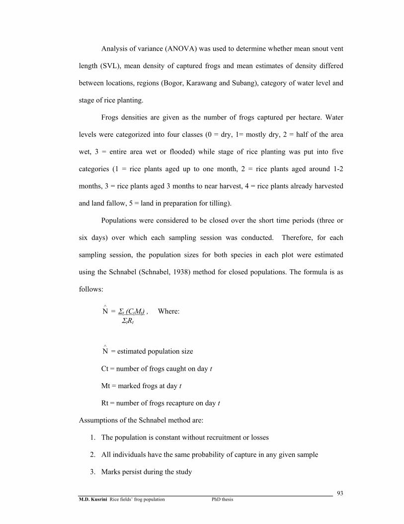
M.D. Kusrini Rice fields’ frog population PhD thesis
93
Analysis of variance (ANOVA) was used to determine whether mean snout vent
length (SVL), mean density of captured frogs and mean estimates of density differed
between locations, regions (Bogor, Karawang and Subang), category of water level and
stage of rice planting.
Frogs densities are given as the number of frogs captured per hectare. Water
levels were categorized into four classes (0 = dry, 1= mostly dry, 2 = half of the area
wet, 3 = entire area wet or flooded) while stage of rice planting was put into five
categories (1 = rice plants aged up to one month, 2 = rice plants aged around 1-2
months, 3 = rice plants aged 3 months to near harvest, 4 = rice plants already harvested
and land fallow, 5 = land in preparation for tilling).
Populations were considered to be closed over the short time periods (three or
six days) over which each sampling session was conducted. Therefore, for each
sampling session, the population sizes for both species in each plot were estimated
using the Schnabel (Schnabel, 1938) method for closed populations. The formula is as
follows:
∧
N = Σt (CtMt) , Where: ΣtRt
∧
N = estimated population size
Ct = number of frogs caught on day t
Mt = marked frogs at day t
Rt = number of frogs recapture on day t
Assumptions of the Schnabel method are:
1. The population is constant without recruitment or losses
2. All individuals have the same probability of capture in any given sample
3. Marks persist during the study
M.D. Kusrini Rice fields’ frog population PhD thesis
94
4. Marking does not affect catchability
The recapture rates of both species for each sampling time were determined by
dividing the number of frogs recaptured from the day before by the total numbers of
frogs captured. For each sampling time, recapture rates were determined for days 2 and
3.
In the movement study, movement distances of individual F. cancrivora were
obtained by calculating distance between mapped capture points. Frogs’ movements
were analysed separately for each sex using three parameters:
1. Distance moved per day
2. Displacement per day
3. The straightness of the movement trail.
Straightness is the ratio of total cumulative distance moved between times the
animal was captured to final displacement from the site of initial capture (Schwarzkopf
and Alford, 2002). It indicates what type of movement pattern frogs are following. A
value of near 1 means that there is a nearly straight path between start and end
observations, whilst 0 indicates that there is little net movement.
5.4 Results
5.4.1 Traits of F. limnocharis-iskandari complex and F. cancrivora
In total, 3671 frogs of eight species were sampled during 2002 and 2003. The
most abundant species was F. limnocharis-iskandari complex (86.4% of individuals)
followed by F. cancrivora (8.9 %) and Occidozyga lima (2.8 %). Bufo melanostictus, B.
biporcatus, B. asper Polypedates leucomystax, and R. chalconota were also
occasionally encountered.

M.D. Kusrini Rice fields’ frog population PhD thesis
95
Except for the first sampling at Subang 2, F. limnocharis-iskandari complex
were always more abundant than F. cancrivora. Overall, I measured and recorded 685
males, 877 females and 1506 juveniles of F. limnocharis-iskandari complex, and 51
males, 95 females and 178 juveniles of F. cancrivora. The mean SVL for female F.
limnocharis-iskandari complex was 36.78 mm (SD = 5.98, range 30.00 - 74.11 mm)
while for males it was 37.96 mm (SD = 5.02, ranges 25.00 - 52.50 mm). Mean SVL for
female F. cancrivora was 53.33 mm (SD = 11.54, ranges 40.00 – 87.86 mm) and for
males was 53.37 mm (SD = 10.47, ranges 35.00 – 75.90 mm). Although mean snout
vent length of females is slightly smaller than that of males, the difference is not
significant, except for F. limnocharis-iskandari complex in Caringin (Table 5-2). The
maximum snout vent lengths of females of both species were greater than the
maximums for males. Figure 5-1 summarizes the SVLs of both species.
Table 5-2. T-tests for sexual dimorphism in snout vent length
F. limnocharis-iskandari complex
F. cancrivora Location
t-statistic P t-statistic P Caringin t862=-5.59 0.000 t27=0.549 0.588 Darmaga t363=0.420 0.675 t9= 0.130 0.160 Karawang-1 t56=2.13 0.038 t18=1.14 0.270 Karawang-2 t110=1.29 0.199 t25=0.341 0.736 Subang-1 t160=1.94 0.055 t16=-0.551 0.590 Subang-2 t62=-0.341 0.734 t37=-0.918 0.364
The mean mass of female F. limnocharis-iskandari complex is 4.40 grams (SD
= 2.54, range 1.19 – 17.40 grams) while for males it is 4.78 grams (SD = 1.59, range
1.10 – 12.30 grams). Mean mass for females of F. cancrivora was 19.47 grams (SD =
14.84, range 2.10 – 105.00 mm) and for males was 17.22 grams (SD = 8.86, range 3.20
– 43.10 grams). All F. limnocharis-iskandari complex and 95.5% of F. cancrivora
captured weighed less than 40 grams; 3.4% of F. cancrivora weighed between 40-80
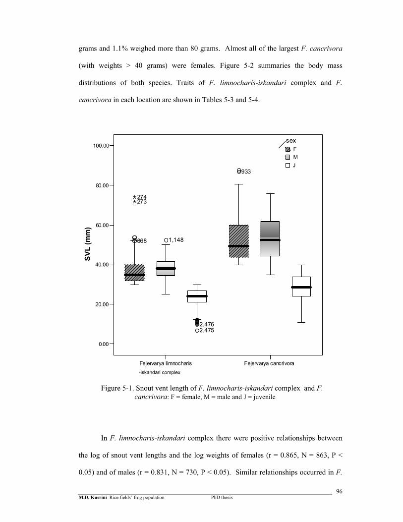
M.D. Kusrini Rice fields’ frog population PhD thesis
96
grams and 1.1% weighed more than 80 grams. Almost all of the largest F. cancrivora
(with weights > 40 grams) were females. Figure 5-2 summaries the body mass
distributions of both species. Traits of F. limnocharis-iskandari complex and F.
cancrivora in each location are shown in Tables 5-3 and 5-4.
Fejervarya limnocharis Fejervarya cancrivora
0.00
20.00
40.00
60.00
80.00
100.00
SVL
(mm
)
868
933
1,148
2,4752,476
273274
sexFMJ
Figure 5-1. Snout vent length of F. limnocharis-iskandari complex and F. cancrivora: F = female, M = male and J = juvenile
In F. limnocharis-iskandari complex there were positive relationships between
the log of snout vent lengths and the log weights of females (r = 0.865, N = 863, P <
0.05) and of males (r = 0.831, N = 730, P < 0.05). Similar relationships occurred in F.
-iskandari complex

M.D. Kusrini Rice fields’ frog population PhD thesis
97
cancrivora (females: r =0.921, N = 90, P < 0.05, males: r =0.908 N = 49, P < 0.05).
These relationships are shown in Figure 5-3.
Fejervarya limnocharis Fejervarya cancrivora
0.00
20.00
40.00
60.00
80.00
Wei
ght (
gram
)
57958886
884
887
892
1,433
1,739
2,465
3,378
272528
897973
1,148
1,886
sexFMJ
Figure 5-2. Body mass of F. limnocharis-iskandari complex and F. cancrivora: F =
female, M = male and J = juvenile
-iskandari complex
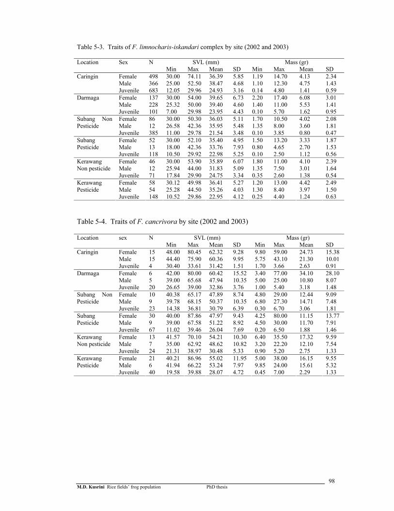
M.D. Kusrini Rice fields’ frog population PhD thesis
98
Table 5-3. Traits of F. limnocharis-iskandari complex by site (2002 and 2003)
SVL (mm) Mass (gr) Location Sex N Min Max Mean SD Min Max Mean SD
Female 498 30.00 74.11 36.39 5.85 1.19 14.70 4.13 2.34 Male 366 25.00 52.50 38.47 4.68 1.10 12.30 4.75 1.43
Caringin
Juvenile 683 12.05 29.96 24.93 3.16 0.14 4.80 1.41 0.59 Female 137 30.00 54.00 39.65 6.73 2.20 17.40 6.08 3.01 Male 228 25.32 50.00 39.40 4.60 1.40 11.00 5.53 1.41
Darmaga
Juvenile 101 7.00 29.98 23.95 4.43 0.10 5.70 1.62 0.95 Female 86 30.00 50.30 36.03 5.11 1.70 10.50 4.02 2.08 Male 12 26.58 42.36 35.95 5.48 1.35 8.00 3.60 1.81
Subang Non Pesticide
Juvenile 385 11.00 29.78 21.54 3.48 0.10 3.85 0.80 0.47 Female 52 30.00 52.10 35.40 4.95 1.50 13.20 3.33 1.87 Male 13 18.00 42.36 33.76 7.93 0.80 4.65 2.70 1.53
Subang Pesticide
Juvenile 118 10.50 29.92 22.98 5.25 0.10 2.50 1.12 0.56 Female 46 30.00 53.90 35.89 6.07 1.80 11.00 4.10 2.39 Male 12 25.94 44.00 31.83 5.09 1.35 7.50 3.01 1.64
Kerawang Non pesticide
Juvenile 71 17.84 29.90 24.75 3.34 0.35 2.60 1.38 0.54 Female 58 30.12 49.98 36.41 5.27 1.20 13.00 4.42 2.49 Male 54 25.28 44.50 35.26 4.03 1.30 8.40 3.97 1.50
Kerawang Pesticide
Juvenile 148 10.52 29.86 22.95 4.12 0.25 4.40 1.24 0.63 Table 5-4. Traits of F. cancrivora by site (2002 and 2003)
SVL (mm) Mass (gr) Location sex N Min Max Mean SD Min Max Mean SD
Female 15 48.00 80.45 62.32 9.28 9.80 59.00 24.73 15.38 Male 15 44.40 75.90 60.36 9.95 5.75 43.10 21.30 10.01
Caringin
Juvenile 4 30.40 33.61 31.42 1.51 1.70 3.66 2.63 0.91 Female 6 42.00 80.00 60.42 15.52 3.40 77.00 34.10 28.10 Male 5 39.00 65.68 47.94 10.35 5.00 25.00 10.80 8.07
Darmaga
Juvenile 20 26.65 39.00 32.86 3.76 1.00 5.40 3.18 1.48 Female 10 40.38 65.17 47.89 8.74 4.80 29.00 12.44 9.09 Male 9 39.78 68.15 50.37 10.35 6.80 27.30 14.71 7.48
Subang Non Pesticide
Juvenile 23 14.38 36.81 30.79 6.39 0.30 6.70 3.06 1.81 Female 30 40.00 87.86 47.97 9.43 4.25 80.00 11.15 13.77 Male 9 39.00 67.58 51.22 8.92 4.50 30.00 11.70 7.91
Subang Pesticide
Juvenile 67 11.02 39.46 26.04 7.69 0.20 6.50 1.88 1.46 Female 13 41.57 70.10 54.21 10.30 6.40 35.50 17.32 9.59 Male 7 35.00 62.92 48.62 10.82 3.20 22.20 12.10 7.54
Kerawang Non pesticide
Juvenile 24 21.31 38.97 30.48 5.33 0.90 5.20 2.75 1.33 Female 21 40.21 86.96 55.02 11.95 5.00 38.00 16.15 9.55 Male 6 41.94 66.22 53.24 7.97 9.85 24.00 15.61 5.32
Kerawang Pesticide
Juvenile 40 19.58 39.88 28.07 4.72 0.45 7.00 2.29 1.33
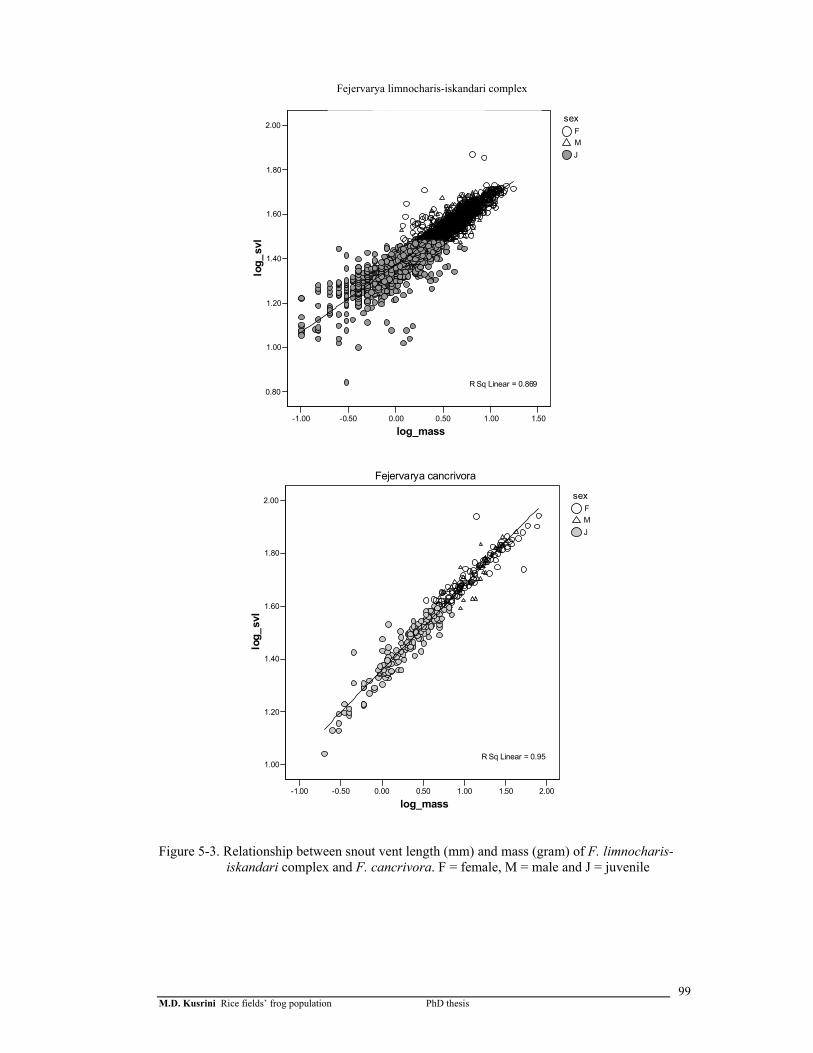
M.D. Kusrini Rice fields’ frog population PhD thesis
99
-1.00 -0.50 0.00 0.50 1.00 1.50
log_mass
0.80
1.00
1.20
1.40
1.60
1.80
2.00
log_
svl
sexFMJ
Fejervarya limnocharis
R Sq Linear = 0.869
-1.00 -0.50 0.00 0.50 1.00 1.50 2.00
log_mass
1.00
1.20
1.40
1.60
1.80
2.00
log_
svl
sexFMJ
Fejervarya cancrivora
R Sq Linear = 0.95
Figure 5-3. Relationship between snout vent length (mm) and mass (gram) of F. limnocharis-iskandari complex and F. cancrivora. F = female, M = male and J = juvenile
Fejervarya limnocharis-iskandari complex
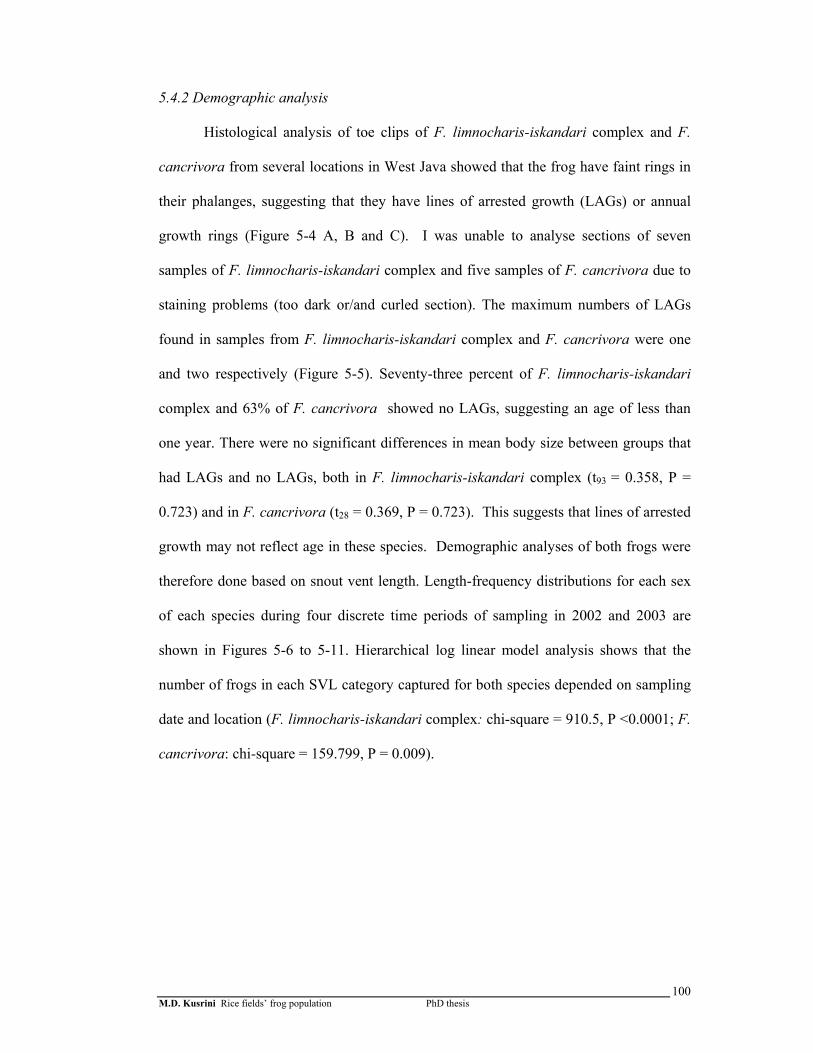
M.D. Kusrini Rice fields’ frog population PhD thesis
100
5.4.2 Demographic analysis
Histological analysis of toe clips of F. limnocharis-iskandari complex and F.
cancrivora from several locations in West Java showed that the frog have faint rings in
their phalanges, suggesting that they have lines of arrested growth (LAGs) or annual
growth rings (Figure 5-4 A, B and C). I was unable to analyse sections of seven
samples of F. limnocharis-iskandari complex and five samples of F. cancrivora due to
staining problems (too dark or/and curled section). The maximum numbers of LAGs
found in samples from F. limnocharis-iskandari complex and F. cancrivora were one
and two respectively (Figure 5-5). Seventy-three percent of F. limnocharis-iskandari
complex and 63% of F. cancrivora showed no LAGs, suggesting an age of less than
one year. There were no significant differences in mean body size between groups that
had LAGs and no LAGs, both in F. limnocharis-iskandari complex (t93 = 0.358, P =
0.723) and in F. cancrivora (t28 = 0.369, P = 0.723). This suggests that lines of arrested
growth may not reflect age in these species. Demographic analyses of both frogs were
therefore done based on snout vent length. Length-frequency distributions for each sex
of each species during four discrete time periods of sampling in 2002 and 2003 are
shown in Figures 5-6 to 5-11. Hierarchical log linear model analysis shows that the
number of frogs in each SVL category captured for both species depended on sampling
date and location (F. limnocharis-iskandari complex: chi-square = 910.5, P <0.0001; F.
cancrivora: chi-square = 159.799, P = 0.009).

M.D. Kusrini Rice fields’ frog population PhD thesis
101
Figure 5-4A. Female F. limnocharis-iskandari complex (SVL = 41.5 mm, mass = 5 g), 1 LAG
(arrow): scale 40 µm
Figure 5-4B. Male F. limnocharis-iskandari complex, no LAGs, SVL = 43 mm, mass = 6.4 g.
(MC = Marrow cavity; EB = Endosteal Bone; PM = Periosteal Bone)
MCEB
PB

M.D. Kusrini Rice fields’ frog population PhD thesis
102
Figure 5-4C. Female F. cancrivora (SVL = 42 mm, mass = 4.6 g); LAG (arrow) = 1
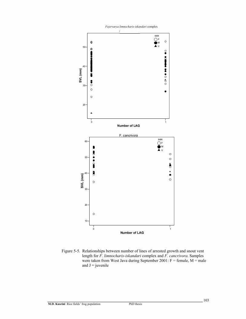
M.D. Kusrini Rice fields’ frog population PhD thesis
103
0 1
Number of LAG
20
30
40
50
SVL
(mm
)
sexFMU
F. limnocharis
0 1
Number of LAG
10
20
30
40
50
60
SVL
(mm
)
sexFMU
F. cancrivora
Figure 5-5. Relationships between number of lines of arrested growth and snout vent
length for F. limnocharis-iskandari complex and F. cancrivora. Samples were taken from West Java during September 2001: F = female, M = male and J = juvenile
Fejervarya limnocharis-iskandari complex
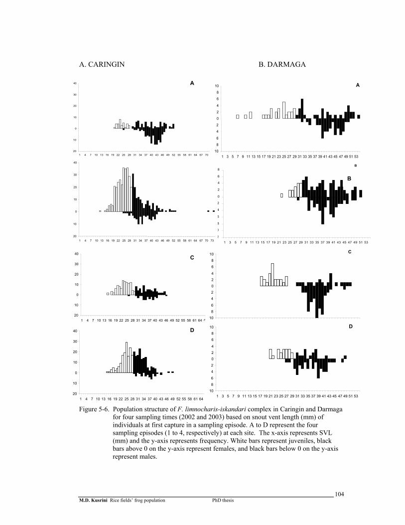
M.D. Kusrini Rice fields’ frog population PhD thesis
104
A. CARINGIN B. DARMAGA
Figure 5-6. Population structure of F. limnocharis-iskandari complex in Caringin and Darmaga
for four sampling times (2002 and 2003) based on snout vent length (mm) of individuals at first capture in a sampling episode. A to D represent the four sampling episodes (1 to 4, respectively) at each site. The x-axis represents SVL (mm) and the y-axis represents frequency. White bars represent juveniles, black bars above 0 on the y-axis represent females, and black bars below 0 on the y-axis represent males.
12
10
8
6
4
2
0
2
4
6
8
1 3 5 7 9 11 13 15 17 19 21 23 25 27 29 31 33 35 37 39 41 43 45 47 49 51 53
B
12
10
8
6
4
2
0
2
4
6
8
1 3 5 7 9 11 13 15 17 19 21 23 25 27 29 31 33 35 37 39 41 43 45 47 49 51 53
B
20
10
0
10
20
30
40
1 4 7 10 13 16 19 22 25 28 31 34 37 40 43 46 49 52 55 58 61 64 67 70 7320
10
0
10
20
30
40
1 4 7 10 13 16 19 22 25 28 31 34 37 40 43 46 49 52 55 58 61 64 67 70 73
20
10
0
10
20
30
40
1 4 7 10 13 16 19 22 25 28 31 34 37 40 43 46 49 52 55 58 61 64 67 70 7320
10
0
10
20
30
40
1 4 7 10 13 16 19 22 25 28 31 34 37 40 43 46 49 52 55 58 61 64 67 70 73
20
10
0
10
20
30
40
1 4 7 10 13 16 19 22 25 28 31 34 37 40 43 46 49 52 55 58 61 64 67 70 7320
10
0
10
20
30
40
1 4 7 10 13 16 19 22 25 28 31 34 37 40 43 46 49 52 55 58 61 64 67 70 73
20
10
0
10
20
30
40
1 4 7 10 13 16 19 22 25 28 31 34 37 40 43 46 49 52 55 58 61 64 67 70 7320
10
0
10
20
30
40
1 4 7 10 13 16 19 22 25 28 31 34 37 40 43 46 49 52 55 58 61 64 67 70 73
10
8
6
4
2
0
2
4
6
8
10
1 3 5 7 9 11 13 15 17 19 21 23 25 27 29 31 33 35 37 39 41 43 45 47 49 51 53
A
10
8
6
4
2
0
2
4
6
8
10
1 3 5 7 9 11 13 15 17 19 21 23 25 27 29 31 33 35 37 39 41 43 45 47 49 51 53
A
1086
42024
68
10
1 3 5 7 9 11 13 15 17 19 21 23 25 27 29 31 33 35 37 39 41 43 45 47 49 51
C
1086
42024
68
10
1 3 5 7 9 11 13 15 17 19 21 23 25 27 29 31 33 35 37 39 41 43 45 47 49 51
C
1086
42024
68
10
1 3 5 7 9 11 13 15 17 19 21 23 25 27 29 31 33 35 37 39 41 43 45 47 49 51 53
D
1086
42024
68
10
1 3 5 7 9 11 13 15 17 19 21 23 25 27 29 31 33 35 37 39 41 43 45 47 49 51 53
D
A
B
C
D

M.D. Kusrini Rice fields’ frog population PhD thesis
105
A. KARAWANG NP B. KARAWANG P Figure 5-7. Population structure of F. limnocharis-iskandari complex in Karawang NP and
Karawang P for four sampling times (2002 and 2003) based on snout vent length (mm) of individuals at first capture in a sampling episode. A to D represent the four sampling episodes (1 to 4, respectively) at each site. The x-axis represents SVL (mm) and the y-axis represents frequency. White bars represent juveniles, black bars above 0 on the y-axis represent females, and black bars below 0 on the y-axis represent males.
8
6
4
2
0
2
4
6
8
10
1 3 5 7 9 11 13 15 17 19 21 23 25 27 29 31 33 35 37 39 41 43 45 47 49
A
8
6
4
2
0
2
4
6
8
10
1 3 5 7 9 11 13 15 17 19 21 23 25 27 29 31 33 35 37 39 41 43 45 47 49
A
8
6
4
2
0
2
4
6
8
10
1 3 5 7 9 11 13 15 17 19 21 23 25 27 29 31 33 35 37 39 41 43 45 47 49
B
8
6
4
2
0
2
4
6
8
10
1 3 5 7 9 11 13 15 17 19 21 23 25 27 29 31 33 35 37 39 41 43 45 47 49
B
8
6
4
2
0
2
4
6
8
10
1 3 5 7 9 11 13 15 17 19 21 23 25 27 29 31 33 35 37 39 41 43 45 47 49
C
8
6
4
2
0
2
4
6
8
10
1 3 5 7 9 11 13 15 17 19 21 23 25 27 29 31 33 35 37 39 41 43 45 47 49
C
8
6
4
2
0
2
4
6
8
10
1 3 5 7 9 11 13 15 17 19 21 23 25 27 29 31 33 35 37 39 41 43 45 47 49
D
8
6
4
2
0
2
4
6
8
10
1 3 5 7 9 11 13 15 17 19 21 23 25 27 29 31 33 35 37 39 41 43 45 47 49
D
4
2
0
2
4
6
8
1 3 5 7 9 11 13 15 17 19 21 23 25 27 29 31 33 35 37 39 41 43 45 47 49 51 53
A
4
2
0
2
4
6
8
1 3 5 7 9 11 13 15 17 19 21 23 25 27 29 31 33 35 37 39 41 43 45 47 49 51 53
A
4
2
0
2
4
6
8
1 3 5 7 9 11 13 15 17 19 21 23 25 27 29 31 33 35 37 39 41 43 45 47 49 51 53
B
4
2
0
2
4
6
8
1 3 5 7 9 11 13 15 17 19 21 23 25 27 29 31 33 35 37 39 41 43 45 47 49 51 53
B
4
2
0
2
4
6
8
1 3 5 7 9 11 13 15 17 19 21 23 25 27 29 31 33 35 37 39 41 43 45 47 49 51 53
C
4
2
0
2
4
6
8
1 3 5 7 9 11 13 15 17 19 21 23 25 27 29 31 33 35 37 39 41 43 45 47 49 51 53
C
4
2
0
2
4
6
8
1 3 5 7 9 11 13 15 17 19 21 23 25 27 29 31 33 35 37 39 41 43 45 47 49 51 53
D
4
2
0
2
4
6
8
1 3 5 7 9 11 13 15 17 19 21 23 25 27 29 31 33 35 37 39 41 43 45 47 49 51 53
D
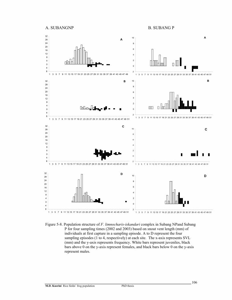
M.D. Kusrini Rice fields’ frog population PhD thesis
106
A. SUBANGNP B. SUBANG P Figure 5-8. Population structure of F. limnocharis-iskandari complex in Subang NPand Subang
P for four sampling times (2002 and 2003) based on snout vent length (mm) of individuals at first capture in a sampling episode. A to D represent the four sampling episodes (1 to 4, respectively) at each site. The x-axis represents SVL (mm) and the y-axis represents frequency. White bars represent juveniles, black bars above 0 on the y-axis represent females, and black bars below 0 on the y-axis represent males.
840
48
121620
242832
1 3 5 7 9 11 13 15 17 19 21 23 25 27 29 31 33 35 37 39 41 43 45 47 49
A
840
48
121620
242832
1 3 5 7 9 11 13 15 17 19 21 23 25 27 29 31 33 35 37 39 41 43 45 47 49
A
840
48
121620
242832
1 3 5 7 9 11 13 15 17 19 21 23 25 27 29 31 33 35 37 39 41 43 45 47 49 51
B
840
48
121620
242832
1 3 5 7 9 11 13 15 17 19 21 23 25 27 29 31 33 35 37 39 41 43 45 47 49 51
B
840
48
121620
242832
1 3 5 7 9 11 13 15 17 19 21 23 25 27 29 31 33 35 37 39 41 43 45 47 49 51
C
840
48
121620
242832
1 3 5 7 9 11 13 15 17 19 21 23 25 27 29 31 33 35 37 39 41 43 45 47 49 51
C
8
4
0
4
8
12
16
20
24
28
32
1 3 5 7 9 11 13 15 17 19 21 23 25 27 29 31 33 35 37 39 41 43 45 47 49 51
D
8
4
0
4
8
12
16
20
24
28
32
1 3 5 7 9 11 13 15 17 19 21 23 25 27 29 31 33 35 37 39 41 43 45 47 49 51
D
2
0
2
4
6
8
10
1 3 5 7 9 11 13 15 17 19 21 23 25 27 29 31 33 35 37 39 41 43 45 47 49 51
A
2
0
2
4
6
8
10
1 3 5 7 9 11 13 15 17 19 21 23 25 27 29 31 33 35 37 39 41 43 45 47 49 51
A
2
0
2
4
6
8
10
1 3 5 7 9 11 13 15 17 19 21 23 25 27 29 31 33 35 37 39 41 43 45 47 49 51
B
2
0
2
4
6
8
10
1 3 5 7 9 11 13 15 17 19 21 23 25 27 29 31 33 35 37 39 41 43 45 47 49 51
B
2
0
2
4
6
8
10
1 3 5 7 9 11 13 15 17 19 21 23 25 27 29 31 33 35 37 39 41 43 45 47 49 51
C
2
0
2
4
6
8
10
1 3 5 7 9 11 13 15 17 19 21 23 25 27 29 31 33 35 37 39 41 43 45 47 49 51
C
2
0
2
4
6
8
10
1 3 5 7 9 11 13 15 17 19 21 23 25 27 29 31 33 35 37 39 41 43 45 47 49 51
D
2
0
2
4
6
8
10
1 3 5 7 9 11 13 15 17 19 21 23 25 27 29 31 33 35 37 39 41 43 45 47 49 51
D
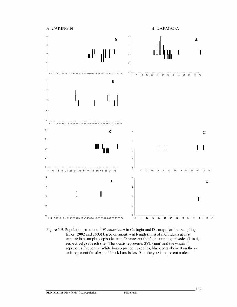
M.D. Kusrini Rice fields’ frog population PhD thesis
107
A. CARINGIN B. DARMAGA Figure 5-9. Population structure of F. cancrivora in Caringin and Darmaga for four sampling
times (2002 and 2003) based on snout vent length (mm) of individuals at first capture in a sampling episode. A to D represent the four sampling episodes (1 to 4, respectively) at each site. The x-axis represents SVL (mm) and the y-axis represents frequency. White bars represent juveniles, black bars above 0 on the y-axis represent females, and black bars below 0 on the y-axis represent males.
4
2
0
2
4
1 4 7 10 13 16 19 22 25 28 31 34 37 40 43 46 49 52 55 58 61 64 67 70 73 76 79
A
4
2
0
2
4
1 4 7 10 13 16 19 22 25 28 31 34 37 40 43 46 49 52 55 58 61 64 67 70 73 76 79
A
4
2
0
2
4
1 6 11 16 21 26 31 36 41 46 51 56 61 66 71 76
C
4
2
0
2
4
1 6 11 16 21 26 31 36 41 46 51 56 61 66 71 76
C
4
2
0
2
4
1 4 7 10 13 16 19 22 25 28 31 34 37 40 43 46 49 52 55 58 61 64 67 70 73 76 79
B
4
2
0
2
4
1 4 7 10 13 16 19 22 25 28 31 34 37 40 43 46 49 52 55 58 61 64 67 70 73 76 79
B
4
2
0
2
4
1 4 7 10 13 16 19 22 25 28 31 34 37 40 43 46 49 52 55 58 61 64 67 70 73 76 79
D
4
2
0
2
4
1 4 7 10 13 16 19 22 25 28 31 34 37 40 43 46 49 52 55 58 61 64 67 70 73 76 79
D
4
2
0
2
4
1 7 13 19 25 31 37 43 49 55 61 67 73 79
A
4
2
0
2
4
1 7 13 19 25 31 37 43 49 55 61 67 73 79
A
4
2
0
2
4
1 7 13 19 25 31 37 43 49 55 61 67 73 79
C
4
2
0
2
4
1 7 13 19 25 31 37 43 49 55 61 67 73 79
C
4
2
0
2
4
1 7 13 19 25 31 37 43 49 55 61 67 73 79
D
4
2
0
2
4
1 7 13 19 25 31 37 43 49 55 61 67 73 79
D
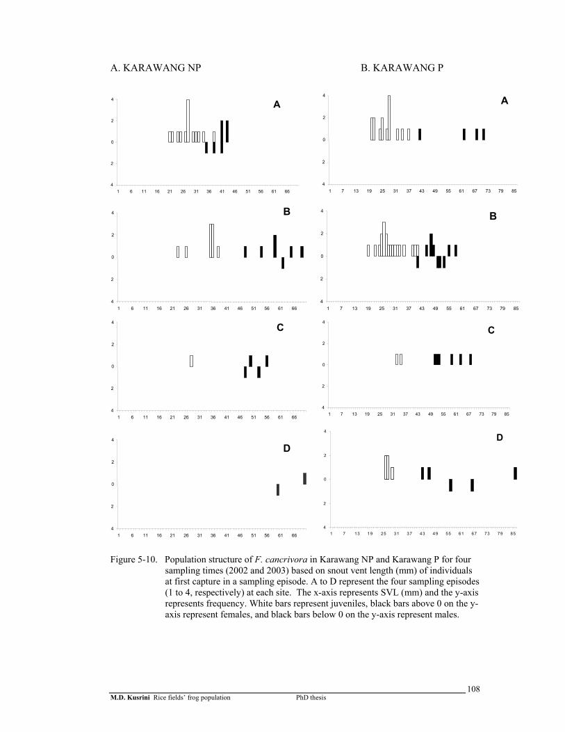
M.D. Kusrini Rice fields’ frog population PhD thesis
108
A. KARAWANG NP B. KARAWANG P Figure 5-10. Population structure of F. cancrivora in Karawang NP and Karawang P for four
sampling times (2002 and 2003) based on snout vent length (mm) of individuals at first capture in a sampling episode. A to D represent the four sampling episodes (1 to 4, respectively) at each site. The x-axis represents SVL (mm) and the y-axis represents frequency. White bars represent juveniles, black bars above 0 on the y-axis represent females, and black bars below 0 on the y-axis represent males.
4
2
0
2
4
1 6 11 16 21 26 31 36 41 46 51 56 61 66
A
4
2
0
2
4
1 6 11 16 21 26 31 36 41 46 51 56 61 66
A
4
2
0
2
4
1 6 11 16 21 26 31 36 41 46 51 56 61 66
B
4
2
0
2
4
1 6 11 16 21 26 31 36 41 46 51 56 61 66
B
4
2
0
2
4
1 6 11 16 21 26 31 36 41 46 51 56 61 66
C
4
2
0
2
4
1 6 11 16 21 26 31 36 41 46 51 56 61 66
C
4
2
0
2
4
1 6 11 16 21 26 31 36 41 46 51 56 61 66
D
4
2
0
2
4
1 6 11 16 21 26 31 36 41 46 51 56 61 66
D
4
2
0
2
4
1 7 13 19 25 31 37 43 49 55 61 67 73 79 85
A
4
2
0
2
4
1 7 13 19 25 31 37 43 49 55 61 67 73 79 85
A
4
2
0
2
4
1 7 13 19 25 31 37 43 49 55 61 67 73 79 85
B
4
2
0
2
4
1 7 13 19 25 31 37 43 49 55 61 67 73 79 85
B
4
2
0
2
4
1 7 13 19 25 31 37 43 49 55 61 67 73 79 85
C
4
2
0
2
4
1 7 13 19 25 31 37 43 49 55 61 67 73 79 85
C
4
2
0
2
4
1 7 13 19 25 31 37 43 49 55 61 67 73 79 85
D
4
2
0
2
4
1 7 13 19 25 31 37 43 49 55 61 67 73 79 85
D
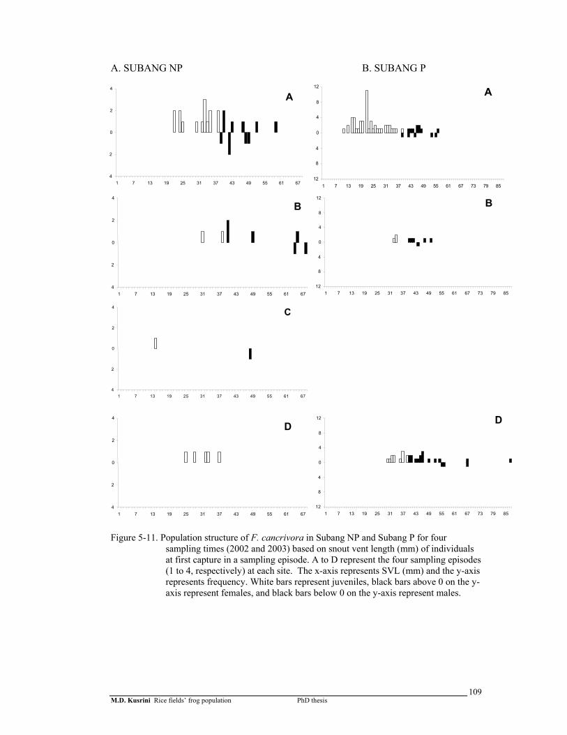
M.D. Kusrini Rice fields’ frog population PhD thesis
109
A. SUBANG NP B. SUBANG P Figure 5-11. Population structure of F. cancrivora in Subang NP and Subang P for four
sampling times (2002 and 2003) based on snout vent length (mm) of individuals at first capture in a sampling episode. A to D represent the four sampling episodes (1 to 4, respectively) at each site. The x-axis represents SVL (mm) and the y-axis represents frequency. White bars represent juveniles, black bars above 0 on the y-axis represent females, and black bars below 0 on the y-axis represent males.
4
2
0
2
4
1 7 13 19 25 31 37 43 49 55 61 67
A
4
2
0
2
4
1 7 13 19 25 31 37 43 49 55 61 67
A
4
2
0
2
4
1 7 13 19 25 31 37 43 49 55 61 67
B
4
2
0
2
4
1 7 13 19 25 31 37 43 49 55 61 67
B
4
2
0
2
4
1 7 13 19 25 31 37 43 49 55 61 67
C
4
2
0
2
4
1 7 13 19 25 31 37 43 49 55 61 67
C
4
2
0
2
4
1 7 13 19 25 31 37 43 49 55 61 67
D
4
2
0
2
4
1 7 13 19 25 31 37 43 49 55 61 67
D
12
8
4
0
4
8
12
1 7 13 19 25 31 37 43 49 55 61 67 73 79 85
A
12
8
4
0
4
8
12
1 7 13 19 25 31 37 43 49 55 61 67 73 79 85
A
12
8
4
0
4
8
12
1 7 13 19 25 31 37 43 49 55 61 67 73 79 85
B
12
8
4
0
4
8
12
1 7 13 19 25 31 37 43 49 55 61 67 73 79 85
B
12
8
4
0
4
8
12
1 7 13 19 25 31 37 43 49 55 61 67 73 79 85
D
12
8
4
0
4
8
12
1 7 13 19 25 31 37 43 49 55 61 67 73 79 85
D
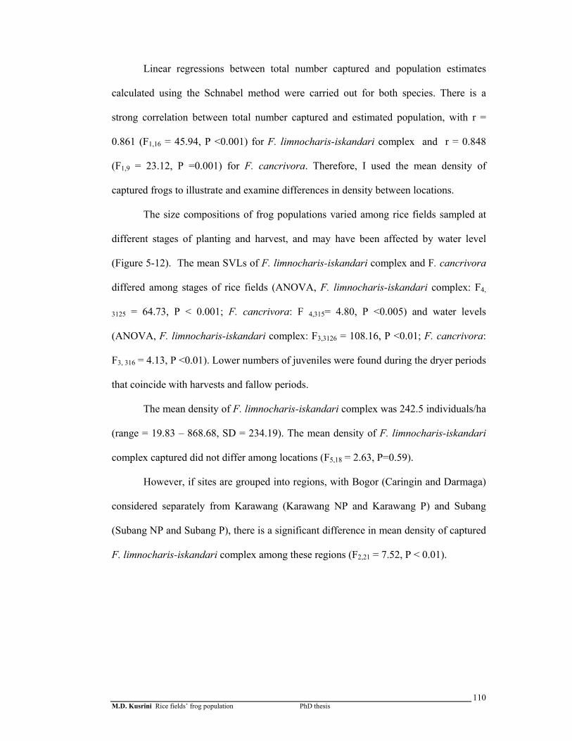
M.D. Kusrini Rice fields’ frog population PhD thesis
110
Linear regressions between total number captured and population estimates
calculated using the Schnabel method were carried out for both species. There is a
strong correlation between total number captured and estimated population, with r =
0.861 (F1,16 = 45.94, P <0.001) for F. limnocharis-iskandari complex and r = 0.848
(F1,9 = 23.12, P =0.001) for F. cancrivora. Therefore, I used the mean density of
captured frogs to illustrate and examine differences in density between locations.
The size compositions of frog populations varied among rice fields sampled at
different stages of planting and harvest, and may have been affected by water level
(Figure 5-12). The mean SVLs of F. limnocharis-iskandari complex and F. cancrivora
differed among stages of rice fields (ANOVA, F. limnocharis-iskandari complex: F4,
3125 = 64.73, P < 0.001; F. cancrivora: F 4,315= 4.80, P <0.005) and water levels
(ANOVA, F. limnocharis-iskandari complex: F3,3126 = 108.16, P <0.01; F. cancrivora:
F3, 316 = 4.13, P <0.01). Lower numbers of juveniles were found during the dryer periods
that coincide with harvests and fallow periods.
The mean density of F. limnocharis-iskandari complex was 242.5 individuals/ha
(range = 19.83 – 868.68, SD = 234.19). The mean density of F. limnocharis-iskandari
complex captured did not differ among locations (F5,18 = 2.63, P=0.59).
However, if sites are grouped into regions, with Bogor (Caringin and Darmaga)
considered separately from Karawang (Karawang NP and Karawang P) and Subang
(Subang NP and Subang P), there is a significant difference in mean density of captured
F. limnocharis-iskandari complex among these regions (F2,21 = 7.52, P < 0.01).

M.D. Kusrini Rice fields’ frog population PhD thesis
111
1284169851170656N =
SPECIES= Fejervarya limnocharis
RICE_OLD
tilling, preparationdry after harvest
near harvestone to tw o month
up to one month
SVL
(mm
)
80
60
40
20
01638
488489
270113372693133828272108
85102945151N =
SPECIES= Fejervarya cancrivora
RICE_OLD
tilling, preparationdry after harvest
near harvestone to tw o month
up to one month
SVL
(mm
)
100
80
60
40
20
0
32073198
3481
475845176149N =
SPECIES= Fejervarya limnocharis
water level
all w etmostly w etpartial drydry
SVL
(mm
)
80
60
40
20
0
2265
488489
159115901592
623321312N =
SPECIES= Fejervarya cancrivora
water level
all w etmostly w etpartial drydry
SVL
(mm
)
100
80
60
40
20
0
32073198
3481
Figure 5-12. Mean size of F. limnocharis-iskandari complex and F. cancrivora in different
stages of planting (top) and water level (bottom)
The mean density of F. cancrivora captured was 32.2 individuals/ha (range: 0 –
230.77, SD: 48.94). The mean density of captured F. cancrivora (n/ha) did not differ
among locations (F5,18 = 1.85, P=0.15) or among regions (F2,21 = 1.52, P=0.24).
The mean density of F. limnocharis-iskandari complex differed among rice
fields at different stages (F4,13 = 6.75, P <0.005) however it did not differ among fields
at different water levels (F3,20 = 1.201, P = 0.404). The mean density of F. cancrivora
did not depend on stage of the rice field (F4,19 = 1.17, P=0.35) or on water level (F3,20 =
0.623, P = 0.609). Figure 5-13 and 5-14 shows the mean density of both species.
-iskandari complex
-iskandari complex

M.D. Kusrini Rice fields’ frog population PhD thesis
112
888N =
LOC_CONV
321
dens
ity c
augh
t all
(n/h
a)
1000
800
600
400
200
0
-200
888N =
LOC_CONV
321
dens
ity c
augh
t all
(n/h
a)
300
200
100
0
-100
21
Figure 5-13. Density of F. limnocharis-iskandari complex (top) and F. cancrivora (bottom)
captured in three regions (1 = Bogor, 2 = Karawang; 3 = Subang).

M.D. Kusrini Rice fields’ frog population PhD thesis
113
73626N =
stage of planting
tilling preparationdry after harvest
near harvestone to tw o months
up to one month
dens
ity c
augh
t all
(n/h
a)
1000
800
600
400
200
0
-20043143N =
water level
all w et and high levw et, but low
partially drydry
dens
ity c
augh
t all
(n/h
a)
1000
800
600
400
200
0
-200
28
83625N =
stage of planting
tilling preparationdry after harvest
near harvestone to tw o months
up to one month
dens
ity c
augh
t all
(n/h
a)
300
200
100
0
-100
9
21
43143N =
water level
all w et and high levw et, but low
partially drydry
dens
ity c
augh
t all
(n/h
a)
300
200
100
0
-100
24
21
Figure 5-14. Density of F. limnocharis-iskandari complex (top) and F. cancrivora
(bottom) captured in various stages of planting and water level during 2002 and 2003.
5.4.3 Sampling effects
The density of frogs differed between the interior and the borders of rice field
blocks; more frogs were found on the edges than in the centre areas (Table 5-5). Mean
densities of frogs captured on the edges wre 0.1007 frogs/m2 (SD = 0.0974, range
0.0030 – 0.2263) for F. limnocharis-iskandari complex and 0.0057 frogs/m2 (SD =
0.0069, range 0.0021 - 0.0160) for F. cancrivora. Mean densities of F. limnocharis-
iskandari complex and F. cancrivora captured on the edges did not differ among
locations (F. limnocharis-iskandari complex: F4,5 = 1.03, P=0.47; F. cancrivora: F3,4 =
0.77, P=0.57).

M.D. Kusrini Rice fields’ frog population PhD thesis
114
Table 5-5. Densities of frogs captured inside paddy field blocks and on their borders. Numbers in brackets indicate the actual number captured.
F. limnocharis-iskandari complex F. cancrivora Location Edge size
(m2) Central size (m2) Edge (n/m) Central (n/m) Edge (n/m) Central (n/m)
Caringin 933 8083.00 0.1747 (163) 0.0697 (491) 0.0021 (2) 0.0007 (6) Darmaga/2003 402.1 1071.40 0.2263 (91) 0.0168 (18) 0.0025 (1) 0 (0) Karawang Pesticide 437.925 6253.38 0.0183 (8) 0.0042 (26) 0.0160 (7) 0.0005 (3) Subang Non Pesticide 933 5667.00 0.0815 (76) 0.0034 (19) 0.0021 (2) 0 (0) Subang Pesticide 675 2185.00 0.0030 (2) 0.0032 (7) 5.4.4 Population estimates
In total 567 males, 747 females and 1425 juveniles of F. limnocharis-iskandari
complex, and 47 males, 92 females and 159 juveniles of F. cancrivora were marked and
released at the six study sites during the period from May 2002 to September 2003.
Recapture rates for both species were low; especially for F. cancrivora in which no
frogs were recaptured more than once (table 5-6). All recaptures occurred within the
three-day sampling episodes. No frogs were recaptured across different sampling
episodes. It was unusual to get any recaptures when the total number of captured frogs
at a site was low (less than about 10). Therefore there were no recaptures from the
lowest density populations.
I performed a series of Fisher’s Exact Tests, one for each site and sampling
period, to determine whether the sex of individuals affected the proportions never
recaptured and recaptured at least once. The distribution of recaptures in both species
mostly does not appear to differ between sexes (P>0.05) except for F. limnocharis-
iskandari complex in Caringin and Subang NP (P<0.05). I used one-way ANOVAs to
test whether recapture rates differed among stages of rice planting and water levels, I
found that the recapture rates of F.limnocharis-iskandari complex did not appear to
depend on stage of rice planting (F 4,67 = 0.65, P = 0.63) or water level (F 3,68 = 0.71, P =
0.55). There were also no significant differences in mean recapture rates of F.
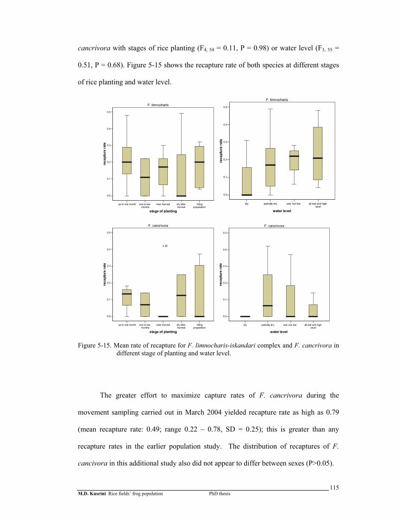
M.D. Kusrini Rice fields’ frog population PhD thesis
115
cancrivora with stages of rice planting (F4, 54 = 0.11, P = 0.98) or water level (F3, 55 =
0.51, P = 0.68). Figure 5-15 shows the recapture rate of both species at different stages
of rice planting and water level.
up to one month one to two months
near harvest dry after harvest
tilling preparation
stage of planting
0.0
0.1
0.2
0.3
0.4
0.5
reca
ptur
e ra
teF. limnocharis
dry partially dry wet, but low all wet and high level
water level
0.0
0.1
0.2
0.3
0.4
0.5
reca
ptur
e ra
te
F. limnocharis
up to one month one to two months
near harvest dry after harvest
tilling preparation
stage of planting
0.0
0.1
0.2
0.3
0.4
0.5
reca
ptur
e ra
te
32
F. cancrivora
dry partially dry wet, but low all wet and high level
water level
0.0
0.1
0.2
0.3
0.4
0.5
reca
ptur
e ra
teF. cancrivora
Figure 5-15. Mean rate of recapture for F. limnocharis-iskandari complex and F. cancrivora in
different stage of planting and water level.
The greater effort to maximize capture rates of F. cancrivora during the
movement sampling carried out in March 2004 yielded recapture rate as high as 0.79
(mean recapture rate: 0.49; range 0.22 – 0.78, SD = 0.25); this is greater than any
recapture rates in the earlier population study. The distribution of recaptures of F.
cancivora in this additional study also did not appear to differ between sexes (P>0.05).
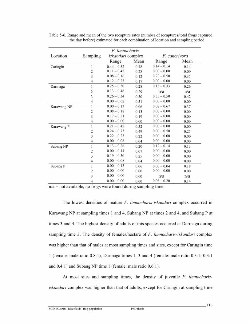
M.D. Kusrini Rice fields’ frog population PhD thesis
116
Table 5-6. Range and mean of the two recapture rates (number of recaptures/total frogs captured
the day before) estimated for each combination of location and sampling period
Location SamplingF. limnocharis-
iskandari complex F. cancrivora Range Mean Range Mean Caringin 1 0.44 – 0.52 0.48 0.14 – 0.14 0.14 2 0.11 – 0.45 0.28 0.00 – 0.00 0.00 3 0.08 – 0.16 0.12 0.20 – 0.50 0.35 4 0.12 – 0.23 0.17 0.00 – 0.00 0.00 Darmaga 1 0.25 – 0.30 0.28 0.18 – 0.33 0.26 2 0.13 – 0.46 0.29 n/a n/a 3 0.26 – 0.34 0.30 0.33 – 0.50 0.42 4 0.00 – 0.62 0.31 0.00 – 0.00 0.00 Karawang NP 1 0.00 – 0.13 0.06 0.08 – 0.67 0.37 2 0.08 – 0.18 0.13 0.00 – 0.00 0.00 3 0.17 – 0.21 0.19 0.00 – 0.00 0.00 4 0.00 – 0.00 0.00 0.00 – 0.00 0.00 Karawang P 1 0.21 – 0.42 0.32 0.00 – 0.00 0.00 2 0.24 – 0.75 0.49 0.00 – 0.50 0.25 3 0.22 – 0.23 0.22 0.00 – 0.00 0.00 4 0.00 – 0.08 0.04 0.00 – 0.00 0.00 Subang NP 1 0.13 – 0.26 0.20 0.12 – 0.14 0.13 2 0.00 – 0.14 0.07 0.00 – 0.00 0.00 3 0.19 – 0.30 0.25 0.00 – 0.00 0.00 4 0.00 – 0.08 0.04 0.00 – 0.00 0.00 Subang P 1 0.00 – 0.13 0.06 0.00 – 0.04 0.18 2 0.00 – 0.00 0.00 0.00 – 0.00 0.00 3 0.00 – 0.00 0.00 n/a n/a 4 0.00 – 0.00 0.00 0.08 – 0.20 0.14
n/a = not available, no frogs were found during sampling time
The lowest densities of mature F. limnocharis-iskandari complex occurred in
Karawang NP at sampling times 1 and 4, Subang NP at times 2 and 4, and Subang P at
times 3 and 4. The highest density of adults of this species occurred at Darmaga during
sampling time 3. The density of females/hectare of F. limnocharis-iskandari complex
was higher than that of males at most sampling times and sites, except for Caringin time
1 (female: male ratio 0.8:1), Darmaga times 1, 3 and 4 (female: male ratio 0.3:1; 0.3:1
and 0.4:1) and Subang NP time 1 (female: male ratio 0.6:1).
At most sites and sampling times, the density of juvenile F. limnocharis-
iskandari complex was higher than that of adults, except for Caringin at sampling time

M.D. Kusrini Rice fields’ frog population PhD thesis
117
1 (adult: juvenile ratio 2:1), Darmaga at times 2 and 4 (adult: juvenile ratio 11:1 and
2:1) and Karawang at time 2 (no juveniles found). In areas where there were no
recaptures (Karawang NP Sampling 2 and 4; Karawang P sampling 1 and 4; Subang NP
sampling 2 and 4 and Subang P sampling 3 and 4) juvenile F. limnocharis-iskandari
complex were always found in low densities (as were adults). Juveniles were found at
the highest densities in Darmaga during sampling time 2. Based on mark recapture
study, the mean densities of F. limnocharis-iskandari complex adults and juveniles
were 193.71/ha (range 29.9 – 695.6) and 588.21/ha (range 0 – 16663.7), respectively.
Table 5-7 shows the estimated population sizes and densities of F. limnocharis-
iskandari complex.
The mean densities of F. cancrivora adults and juveniles were 39.76/ha (range 0
– 107.14) and 85.27/ha (range 0 - 449.05). At most sites and sampling times, the density
of F. cancrivora was low, with no recaptures, or this species was absent. Sufficient F.
cancrivora for population estimates were only found at Caringin at times 1 and 3,
Darmaga at times 1 and 3, Karawang NP at time 1, Karawang P at time 2, and Subang P
at times 2 and 4.
The highest densities of adult and juvenile F. cancrivora were both found in
Subang at sampling time 2. The number of juveniles/hectare was higher than the
number of adults except for Karawang P at sampling time 2 (adult: juvenile ratio 1.82:1)
and Subang P at sampling time 4 (adult: juvenile ratio 1.74:1). Except for Subang P, the
density of F. cancrivora females/hectare was low compared to that of males. Table 5-8
shows the estimated population sizes and densities of F. cancrivora.
M.D. Kusrini Rice fields’ frog population PhD thesis
118
Table 5-7. F. limnocharis-iskandari complex population estimates based on the Schnabel method.
Estimated population size Site (area m2)
Sampling time Male Female Juvenile Adult
F:M ratio
adult density (n/ha)
Juvenile density (n/ha)
Adult: Juvenile ratio
1 118.13 91.85 99.75 204.52 0.8: 1 226.84 110.64 2.05:1 2 135.29 321.38 722.18 244.97 2.4:1 271.70 801.00 0.34:1 3 119.50 161.11 757.20 269.46 1.3:1 298.87 839.84 0.36:1 Caringin
(9,016) 4 72.80 263.88 712.88 335.69 3.6:1 372.33 790.68 0.47:1 1 74.00 23.38 166.50 108.00 0.3:1 103.45 159.48 0.65:1 Darmaga
(10,440) 2 66.45 149.25 17.75 206.84 2.2:1 198.12 17.00 11.65:1 3 92.00 27.17 245.00 102.50 0.3:1 695.62 1662.71 0.42:1 Darmaga
(1,473.5) 4 70.88 28.00 39.71 99.00 0.4:1 671.87 269.52 2.49:1 1 NA** NA** 62.00 NA** NA** NA** 175.65 NA** 2 6.00 15.00 NA** 46.00 2.5:1 130.32 NA** NA** 3 NA** 17.86 266.00 26.43 NA** 74.87 753.61 0.10:1
Karawang NP (3,529.7) 4 NA** NA** NA** NA** NA** NA** NA** NA**
1 44.60 63.00 NA** 101.00 1.4:1 150.94 NA** NA** 2 9.29 12.00 48.00 20.00 1.3:1 29.89 71.73 0.42:1 3 12.00 12.00 162.60 26.67 1.0:1 39.85 243.00 0.16:1
KarawangP (6,691.3) 4 7.00 NA** NA** 80.00 NA** 119.56 NA** NA**
1 20.20 12.50 516.55 33.00 0.6:1 50.00 782.64 0.06:1 2 NA** NA** NA** NA** NA** NA** NA** NA** 3 40.21 116.86 0.00 106.85 2.9:1 161.89 0.00 NA**
Subang NP (6,600) 4 NA** NA** NA** NA** NA** NA** NA** NA**
1 14.00 NA** 317.00 31.00 NA** 108.39 1108.39 0.10:1 2 3.00 26.77 128.43 30.64 8.9:1 107.14 449.05 0.24:1 3 NA** NA** NA** NA** NA** NA** NA** NA** Subang P
(2,860) 4 NA** NA** NA** NA** NA** NA** NA** NA** Note: NA** stands for not available because there were no recaptures at that site at that time

M.D. Kusrini Rice fields’ frog population PhD thesis
119
Table 5-8. F. cancrivora population estimates based on the Schnabel method.
Population size Site (area m2)
Sampling time Male Female Juvenile Adult
F:M ratio
Adult density (n/ha)
Juvenile density (n/ha)
Adult: Juvenile ratio
1 28.50 8.00 0.00 36.75 0.3: 1 40.76 0.00 NA** 2 NA** NA** NA** NA** NA** NA** NA** NA** 3 NA** 3.00 NA** 8.00 NA** 8.87 NA** NA** Caringin
(9,016) 4 NA** NA** NA** NA** NA** NA** NA** NA** 1 4.00 3.00 42.00 7.50 0.8: 1 7.18 40.23 0.18:1 Darmaga
(10,440) 2 NA** NA** NA** NA** NA** NA** NA** NA** 3 0.00 1.00 2.00 1.00 NA** 6.79 13.57 0.50:1 Darmaga
(1,473.5) 4 NA** NA** NA** NA** NA** NA** NA** NA** 1 NA** 1.00 52.00 7 NA** 19.83 147.32 0.13:1 2 NA** NA** NA** NA** NA** NA** NA** NA** 3 NA** NA** NA** NA** NA** NA** NA** NA**
Karawang NP (3,529.7) 4 NA** NA** NA** NA** NA** NA** NA** NA**
1 0.00 0.00 0.00 0.00 NA** 0.00 0.00 NA** 2 NA** 21.00 24.67 45.00 NA** 67.25 36.86 1.82:1 3 NA** NA** NA** NA** NA** NA** NA** NA**
KarawangP (6,691.3) 4 NA** NA** NA** NA** NA** NA** NA** NA**
1 0.00 0.00 0.00 0.00 NA** 0.00 0.00 NA** 2 NA** NA** NA** NA** NA** NA** NA** NA** 3 NA** NA** NA** NA** NA** NA** NA** NA**
Subang NP (6,600) 4 NA** NA** NA** NA** NA** NA** NA** NA**
1 7.00 NA** NA** 128.00 NA** NA** NA** NA** 2 3.00 26.77 128.43 30.64 8.9: 1 107.14 449.05 0.24:1 3 NA** NA** NA** NA** NA** NA** NA** NA** Subang P
(2,860) 4 0.00 40.00 23.00 40.00 NA** 139.86 80.42 1.74:1 Darmaga (4,592.8)
March 2004 30 44 21.60 67.20 1.3:1 146.32 47.03 3.11:1
Note: NA** means not available since there were no recaptures
5.4.5 F. cancrivora movement
Additional sampling I carried out at Darmaga to examine frog movements
resulted in 118 captures of 71 F. cancrivora, consisting of 36 females (mean SVL 58.42
mm, range 40.58 – 95.12 mm, SD = 18.94), 16 males (mean SVL 60.79 mm, range
53.57 – 73.82 mm, SD = 5.81) and 19 juveniles (mean SVL 35.81 mm, range 24.52 –
39.61 mm, SD = 3.66. Twenty-nine frogs (42.6%) were captured more than once, with
two females recaptured after 5 days, two juveniles recaptured after 4 days, and five
frogs recaptured after 3 days (2 females, 2 males and 1 juvenile).
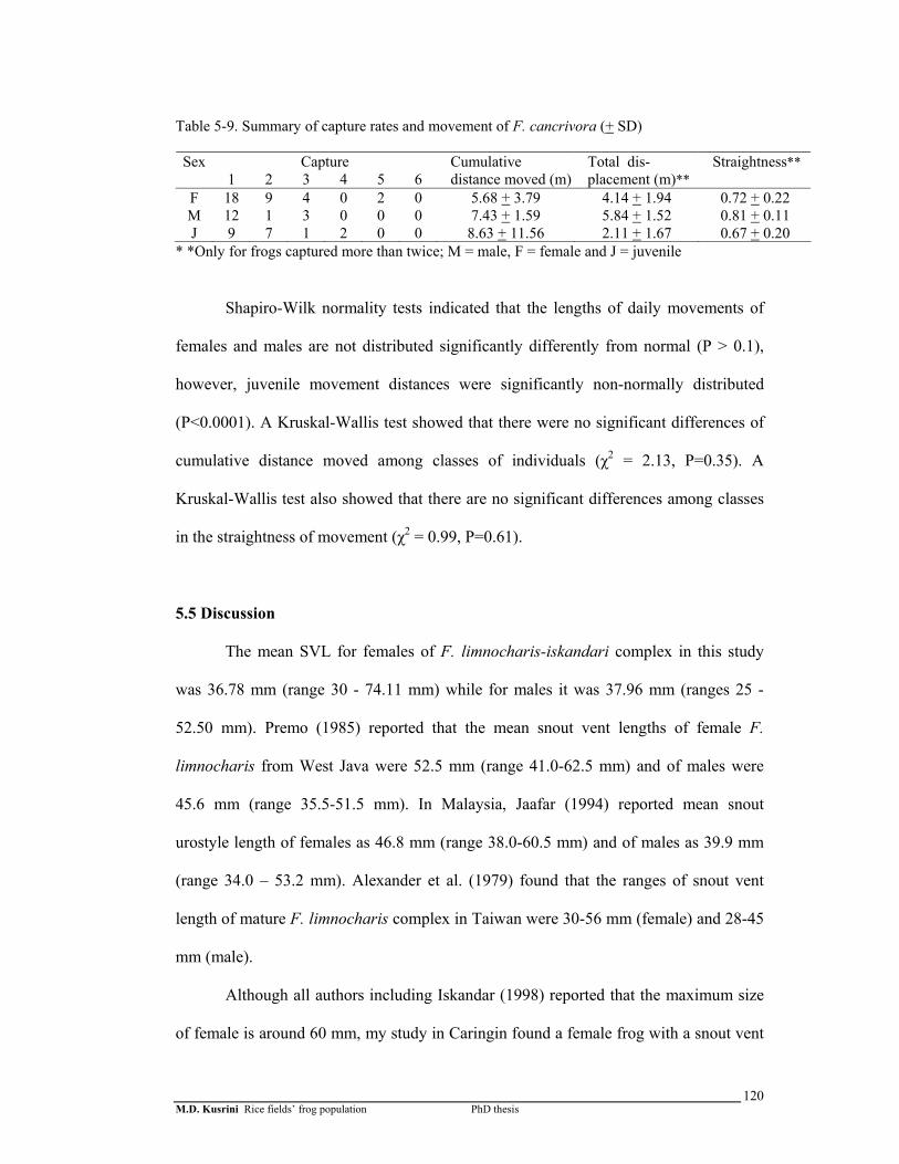
M.D. Kusrini Rice fields’ frog population PhD thesis
120
Table 5-9. Summary of capture rates and movement of F. cancrivora (+ SD)
Capture Sex 1 2 3 4 5 6
Cumulative distance moved (m)
Total dis-placement (m)**
Straightness**
F 18 9 4 0 2 0 5.68 + 3.79 4.14 + 1.94 0.72 + 0.22 M 12 1 3 0 0 0 7.43 + 1.59 5.84 + 1.52 0.81 + 0.11 J 9 7 1 2 0 0 8.63 + 11.56 2.11 + 1.67 0.67 + 0.20
* *Only for frogs captured more than twice; M = male, F = female and J = juvenile
Shapiro-Wilk normality tests indicated that the lengths of daily movements of
females and males are not distributed significantly differently from normal (P > 0.1),
however, juvenile movement distances were significantly non-normally distributed
(P<0.0001). A Kruskal-Wallis test showed that there were no significant differences of
cumulative distance moved among classes of individuals (χ2 = 2.13, P=0.35). A
Kruskal-Wallis test also showed that there are no significant differences among classes
in the straightness of movement (χ2 = 0.99, P=0.61).
5.5 Discussion
The mean SVL for females of F. limnocharis-iskandari complex in this study
was 36.78 mm (range 30 - 74.11 mm) while for males it was 37.96 mm (ranges 25 -
52.50 mm). Premo (1985) reported that the mean snout vent lengths of female F.
limnocharis from West Java were 52.5 mm (range 41.0-62.5 mm) and of males were
45.6 mm (range 35.5-51.5 mm). In Malaysia, Jaafar (1994) reported mean snout
urostyle length of females as 46.8 mm (range 38.0-60.5 mm) and of males as 39.9 mm
(range 34.0 – 53.2 mm). Alexander et al. (1979) found that the ranges of snout vent
length of mature F. limnocharis complex in Taiwan were 30-56 mm (female) and 28-45
mm (male).
Although all authors including Iskandar (1998) reported that the maximum size
of female is around 60 mm, my study in Caringin found a female frog with a snout vent
M.D. Kusrini Rice fields’ frog population PhD thesis
121
lengths of 74.11 mm. During my investigation of the distributions of the study species
(chapter 4), the snout-vent lengths of 1001 specimens which was determined by MZB
curators as F. limnocharis from all over Indonesia stored in the Museum Zoology at
Bogor (MZB) were measured; out of which 762 specimens are from Java. The mean
snout vent length of female F. limnocharis in this Javanese sample was 36.74 mm with
a maximum 75.19 mm (specimen ID 3337 captured 9 September 1988 from Cilember,
Bogor). The mean snout vent length of male F. limnocharis was 37.96 mm with a
maximum of 54.52 mm (specimen ID 142 collected in 1930 from Karimun Jawa). On
average, females in my samples were smaller than those found in the studies by Premo
(1985) and Jaafar (1994), however, my maximum SVLs was greater than the maxima
reported by them and also by Alexander et al. (1979). This suggests that the smaller
average size of females in my study may reflect poorer growth conditions or higher
rates of loss among larger individuals, rather than inherent size differences between the
populations in my study and the other studies.
The mean SVL of female F. cancrivora in my population study was 53.33 mm
(range 40 – 87.86 mm) and for males was 53.37 mm (range 35 – 75.90 mm). Church
(1960) gave the range of snout vent length of F. cancrivora from Jakarta and Karawang
as 64-132 mm (females) and 61-93 mm (males), while Premo gave the mean of male
snout vent length as 76.7 mm (range 59.0-87.0 mm) and that of females as 98.6 mm
(range 68.0-119.0 mm). According to Jaafaar (1994) the mean snout urostyle length of
female F. cancrivora in Malaysia was 66.0 mm (range 45.1-104.2) and of males was
61.0 mm (range 40.5-86.2 mm). My measurements of 484 specimens of F. cancrivora
from all over Indonesia stored in the MZB indicate that the mean snout vent length of
females was 62.30 mm (maximum 98.45 mm, specimen ID 2070 captured 6 April 1965
M.D. Kusrini Rice fields’ frog population PhD thesis
122
from Bogor Botanical Garden, Bogor) and for males was 61.07 mm (maximum 86.49
mm, specimen ID 477.4 captured 6 December 1954 from Bogor).
The body sizes of frogs depend on several factors such as season, food
availability and predation (Duellman and Trueb, 1986). However, in the case of F.
cancrivora, both Church (1960) and Premo (1985) recorded the size of frogs captured
by professional harvesters, and thus their data were probably biased towards larger body
sizes, since professional harvesters usually only catch larger frogs. The means and
ranges of body size I found in my population samples are substantially smaller than the
sizes I found in samples from the catches of professional frog hunters working in Java
(Table 3-2); in those samples the mean and range for adult male and female F.
cancrivora were 65.54 mm (50.20 to 86.20 mm) and 75.10 mm (40.00-162.00 mm),
respectively. This differences illustrates the fact that professional hunters concentrate a
disproportionate share of harvesting effort on the largest individuals in populations, and
also suggests that my population samples may be biased towards smaller, easier-to-
catch individuals.
Most previous authors have suggested that both study species exhibit sexual size
dimorphism, with females larger than males. In my results for both species, females
tended to be slightly smaller than males although the differences in size are not
significant. However, the largest individuals of both species found in my study were
females. Since all of my sampling areas were subject to extensive hunting by frog
harvesters, it is possible that larger frogs, which might mostly be females, were largely
absent due to hunting pressures.
There have been no previous efforts to use skeletochronology on Indonesian
frogs. Most successful skeletochronological work has been done on temperate species
(e.g Halliday and Verrel, 1988; Ryser, 1988; Reaser, 2000). Tropical frogs in North
M.D. Kusrini Rice fields’ frog population PhD thesis
123
Queensland (Felton, 1999) and in India (Kumbar and Pancharatna, 2001) also show
annual growth patterns in their bones. My skeletochronological results did not indicate
that frogs with different numbers of LAGs (only 0 or 1) were different sizes, suggesting
that the number of LAGs may not be related to age in these species. The difference
between my results and those in other tropical systems may be related to the seasonality
of temperature. North Queensland and India have marked temperature differences
between dry (winter) and wet (summer) seasons, whereas no marked differences occur
in West Java.
The density of frogs differed among locations. Results showed that both F.
limnocharis-iskandari complex and F. cancrivora were found more on the edges than
on the central areas of rice blocks. Some of this difference may be caused by sampling
bias; it is harder to locate and capture frogs in the central areas of rice fields,
particularly during the later stages of the rice planting cycle, when plants are large and
dense. This may lead to underestimates of population size, particularly for larger
individuals, which are faster and more wary.
Bogor rice fields had the densest frog populations, followed by Subang and
Karawang. Most Bogor rice fields depended on surface runoff since rainfall occurs
throughout the year. Rice planting can occur as often as three times a year, compared to
rice fields in Subang and Karawang which only are planted twice a year. Paddy fields in
Subang and Karawang usually rely on irrigation and during fallow periods the area can
be very dry. Environmental conditions in Bogor are more suitable for both of the study
species and recruitment occurs during most stages of planting as shown in Figure 5-14.
The population structure of both species fluctuated with the stages of rice
planting. More smaller frogs were found during tilling and the earlier stages of rice
growth, whereas larger frogs were found towards the end of the planting season,
M.D. Kusrini Rice fields’ frog population PhD thesis
124
especially during harvest and fallow periods which largely coincide with lower water
levels and dry periods. It appears that the timing of recruitment coincides with water
level, in accordance with Jaafar et al. (1999) findings in Malaysian rice fields.
Although the breeding patterns of F. limnocharis-iskandari complex and F.
cancrivora seemed correlated with the rice planting stage, the lack of distinct annual
LAGs in the skeletochronological data suggests that both species grow throughout the
year. It is also possible that these frogs do not live long. If paddy field frogs in West
Java grow on average according to Jaafar’s (1994) equations for growth of F.
limnocharis and F. cancrivora in Malaysia, the ages of F. limnocharis-iskandari
complex and F. cancrivora in this sample would range from 1 week to 21 months (1.9
years) (F. limnocharis-iskandari complex) and 1 week to 1 year (F. cancrivora). Given
the absence of larger F. cancrivora in my samples, which suggests that older individuals
are absent from my populations, it seems that the populations of F. cancrivora I
examined tend to be biased towards young mature frogs. Since F. cancrivora is more
heavily exploited than F. limnocharis-iskandari complex the biased population size
distribution of F. cancrivora suggests that harvesting may be at or near maximum
sustainable rates. If almost all older individuals are removed from the populations by
harvesting, it is likely that the growth rates of the populations are being negatively
affected.
Most previous works on rice field frog populations has focused on their breeding
biology (Church, 1960; Alexander et al., 1963 and 1979; Premo, 1985; Jaafar et al.,
1999) and has not mentioned the size of the area sampled when reporting the numbers
of frogs captured, thus providing no information on the density of frogs. Two studies
have provided enough information to allow comparisons with my data. Jaafar (1994)
and Dash and Mahanta (1993) both collected frogs for three hours per sampling night
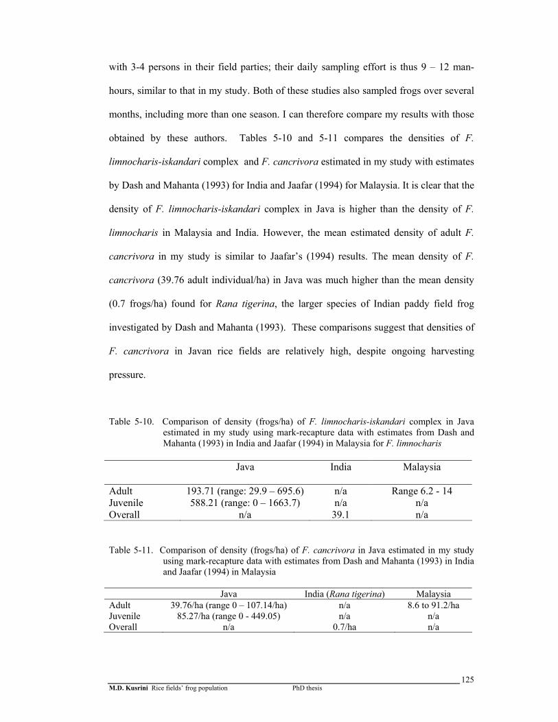
M.D. Kusrini Rice fields’ frog population PhD thesis
125
with 3-4 persons in their field parties; their daily sampling effort is thus 9 – 12 man-
hours, similar to that in my study. Both of these studies also sampled frogs over several
months, including more than one season. I can therefore compare my results with those
obtained by these authors. Tables 5-10 and 5-11 compares the densities of F.
limnocharis-iskandari complex and F. cancrivora estimated in my study with estimates
by Dash and Mahanta (1993) for India and Jaafar (1994) for Malaysia. It is clear that the
density of F. limnocharis-iskandari complex in Java is higher than the density of F.
limnocharis in Malaysia and India. However, the mean estimated density of adult F.
cancrivora in my study is similar to Jaafar’s (1994) results. The mean density of F.
cancrivora (39.76 adult individual/ha) in Java was much higher than the mean density
(0.7 frogs/ha) found for Rana tigerina, the larger species of Indian paddy field frog
investigated by Dash and Mahanta (1993). These comparisons suggest that densities of
F. cancrivora in Javan rice fields are relatively high, despite ongoing harvesting
pressure.
Table 5-10. Comparison of density (frogs/ha) of F. limnocharis-iskandari complex in Java estimated in my study using mark-recapture data with estimates from Dash and Mahanta (1993) in India and Jaafar (1994) in Malaysia for F. limnocharis
Java
India Malaysia
Adult 193.71 (range: 29.9 – 695.6) n/a Range 6.2 - 14 Juvenile 588.21 (range: 0 – 1663.7) n/a n/a Overall n/a 39.1 n/a
Table 5-11. Comparison of density (frogs/ha) of F. cancrivora in Java estimated in my study using mark-recapture data with estimates from Dash and Mahanta (1993) in India and Jaafar (1994) in Malaysia
Java India (Rana tigerina) Malaysia Adult 39.76/ha (range 0 – 107.14/ha) n/a 8.6 to 91.2/ha Juvenile 85.27/ha (range 0 - 449.05) n/a n/a Overall n/a 0.7/ha n/a
M.D. Kusrini Rice fields’ frog population PhD thesis
126
Some studies of stream-dwelling frogs have shown that these species have site
fidelity (Tessier et al., 1991; Kam and Chen 2000). Other studies have shown that some
species migrate seasonally for breeding (Dole and Durant, 1974; Beshkov and Jameson,
1984), and others lack philopatry and move nomadically (Schwarzkopf and Alford,
2002). In my study many individuals were captured only once and I never captured
frogs marked from previous sampling occasions, even when these were only one month
apart. The environment in rice fields fluctuates frequently in terms of water level and
cover (rice plants). Rice in Java is usually planted in large aggregations of rice fields,
consisting of hundreds or sometimes thousands of hectares of individual paddy fields
owned by different farmers. Each aggregation of rice fields often includes fields in
different stages of plant development and water level. Frogs are likely to move between
fields to avoid unfavourable environments, such as dry habitats. Most of the lower
capture rates in my study occurred during fallow periods, in which the soil in dry fields
in areas such as Karawang and Subang was so dry that it cracked. My low recapture
rates, even over relatively short time periods with relatively high sampling effort,
suggest that both F. limnocharis-iskandari complex and F. cancrivora may behave
similarly to Bufo marinus in Australia, which are nomadic (Schwarzkopf and Alford,
2002). They may remain in an area of habitat while conditions are favourable, but
move on when they become unfavourable, and not return.
F. cancrivora is the most commonly harvested frog in Java. The low numbers
of F. cancrivora captured and recaptured in all six paddy fields could suggest that
population sizes of this species are low. However, the densities I estimated when mark-
recapture calculations were possible were similar to those found by Jaafar (1994) for
unharvested Malaysian populations. In my movement study, which involved more
intensive sampling effort over a 6-day period, I captured greater numbers of frogs,
M.D. Kusrini Rice fields’ frog population PhD thesis
127
suggesting that some of the lower counts I obtained were underestimates of density
caused by low catchability of frogs. The results of the movement aspect of this study
showed that F. cancrivora tend to move in relatively straight lines, suggesting that
individuals may frequently disperse between rice fields. This must account for the
absence of long-term recaptures, which could not be caused entirely by mortality, as
that would require that most adults die between each monthly sample, which would lead
to rapid extinction of populations. The relatively small sizes of adults I captured, when
compared to the same species in other regions and to samples obtained from frog
hunters, suggests that harvesting may be removing a large proportion of the larger
adults from the populations, which could lead to reduced rates of recruitment. This may
also reflect in part lower catchability of larger frogs, which are probably captured more
efficiently by frog hunters than by biologists. Although I obtained sufficient data to
allow initial evaluations of the status of populations of F. cancrivora and F.
limnocharis-iskandari complex, additional work will be needed to fully understand the
dynamics of these species.
M.D. Kusrini L. macrodon population biology PhD thesis
128
CHAPTER 6
THE POPULATION BIOLOGY OF LIMNONECTES MACRODON
6.1 Introduction
The Giant Javanese frog, Limnonectes macrodon, is commonly harvested for
human consumption in Indonesia, especially in West Java (Chapter 3). This frog is a
member of the ranid fanged frogs, which inhabit tropical and subtropical Asia, and is
unique among anurans in that the males do not have the usual secondary sexual
characteristics such as nuptial pads and voice (Inger, 1969). Known previously as Rana
macrodon, the taxonomic status of this species has undergone several revisions and it
has been divided into several other species, such as Limnonectes blythii, L. malesianus,
L. leporinus, L. ingeri and L. kadarsani (Iskandar, 1998). A pioneer study by Sugiri in
1979 provided information on the basic biology of the Rana blythii complex in West
Java, which is now known as Limnonectes macrodon (Iskandar, pers. comm., see
Chapter 4). As with most Indonesian frogs, although it is common very little is known
of its ecology, life history, or behavioural traits. This makes it difficult to assess the
impact of harvesting on this species.
The objective of this study was to assess the population biology of Limnonectes
macrodon at two streams in West Java: Cilember and Ciapus Leutik. Additional data on
the biology of the species was taken from frogs captured by professional hunters.
6.2 Methods
6.2.1 Location
A single 400 m transect was established at both the Cilember (∼30 km south of
Bogor) and the Ciapus Leutik (∼10 km west of Bogor) streams. Maps and detailed site
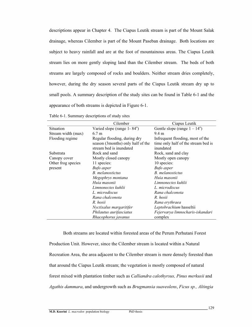
M.D. Kusrini L. macrodon population biology PhD thesis
129
descriptions appear in Chapter 4. The Ciapus Leutik stream is part of the Mount Salak
drainage, whereas Cilember is part of the Mount Paseban drainage. Both locations are
subject to heavy rainfall and are at the foot of mountainous areas. The Ciapus Leutik
stream lies on more gently sloping land than the Cilember stream. The beds of both
streams are largely composed of rocks and boulders. Neither stream dries completely,
however, during the dry season several parts of the Ciapus Leutik stream dry up to
small pools. A summary description of the study sites can be found in Table 6-1 and the
appearance of both streams is depicted in Figure 6-1.
Table 6-1. Summary descriptions of study sites
Cilember Ciapus Leutik Situation Varied slope (range 1- 84o) Gentle slope (range 1 – 14o) Stream width (max) 6.7 m 9.4 m Flooding regime Regular flooding, during dry
season (3months) only half of the stream bed is inundated
Infrequent flooding, most of the time only half of the stream bed is inundated
Substrata Rock and sand Rock, sand and clay Canopy cover Mostly closed canopy Mostly open canopy Other frog species present
11 species: Bufo asper B. melanostictus Megophrys montana Huia masonii Limnonectes kuhlii L. microdiscus Rana chalconota R. hosii Nyctixalus margaritifer Philautus aurifasciatus Rhacophorus javanus
10 species: Bufo asper B. melanostictus Huia masonii Limnonectes kuhlii L. microdiscus Rana chalconota R. hosii Rana erythraea Leptobrachium hasseltii Fejervarya limnocharis-iskandari complex
Both streams are located within forested areas of the Perum Perhutani Forest
Production Unit. However, since the Cilember stream is located within a Natural
Recreation Area, the area adjacent to the Cilember stream is more densely forested than
that around the Ciapus Leutik stream; the vegetation is mostly composed of natural
forest mixed with plantation timber such as Calliandra calothyrsus, Pinus merkusii and
Agathis dammara, and undergrowth such as Brugmansia suaveolens, Ficus sp., Altingia

M.D. Kusrini L. macrodon population biology PhD thesis
130
excelsa, Achasma megalochilos, Selaginella plana, Artocarpus heterophyllus,
Melastoma malabathricum, Acacia sp., Daemonorops rubra and bamboo (Bambusa
sp.).
Figure 6-1. The Ciapus Leutik stream (left ) and the Cilember stream (right)
The Cilember stream lies between 662 and 840 m above sea level (asl). It has a
steep gradient and is interrupted by seven waterfalls ranging in height from one metre to
more than 15 m high. In the Cilember stream transect the first 200 m lies mostly near
the lower elevation (662 m a.s.l.), with a shallow gradient. A 15 m high waterfall
divides this from the next 100 m. This is followed by a 5 m high waterfall and the final
100 m of the transect. The Cilember stream eventually flows into the Ciliwung River
and flows to the city of Bogor.
The elevation of the Ciapus Leutik stream is between 709 and 717 m. As with
the Cilember stream, the lower 200 m of the transect is divided from the upper 200 m

M.D. Kusrini L. macrodon population biology PhD thesis
131
by a small waterfall, around 3 m high. Half of the area along the transect in the Ciapus
Leutik stream is within a forest maintained for harvest by the nearby villages (a
community forest). As such, the vegetation is mainly Pinus merkusii with undergrowth
of a vegetable plant Buchanaria arborescens. Other vegetation found in the area
includes timber and crops such as Piper aduncum, Bambusa sp., Eupatorium odorata,,
Tetraria sp., Calliandra calothyrsus, Amomum sp., Selaginella plana, Paraserianthes
falcataria, Mesopsis eminii, Ageratum conyzoides, Brugmansia suaveolens, Vitis sp.,
and Lantana cammara, planted by inhabitants from the nearby village. As with the
Cilember stream, the water from the Ciapus Leutik stream flows to Bogor.
Access to the area inside the Cilember Natural Recreation Unit is restricted to
visitors and Perum Perhutani (Perusahaan Umum Perhutanan Indonesia or Indonesian
Forest Product Company) officers, whereas access to Ciapus Leutik is open. Figure 6-1
shows the condition of the Cilember and Ciapus Leutik streams.
6.2.2 Sampling
Two days of sampling were conducted at each site during each month from June
2002 to May 2003, inclusive (a continuous 12 month sampling period); additional
sampling was carried out in January, April and July 2004. Sampling began during the
evening, starting around 19.30, and continued until around 01.00 the next morning. At
least 2 people took part in each survey. A thorough search was made for frogs along the
entire length of each transect and within 1 m of each side of the streams for a total of
683-man hours for all samples, or around 11-man hours per sampling day. For each frog
captured we recorded snout vent length (SVL), weight, microhabitat, position along the
transect with reference to markers along the transect, the activity of each individual
captured at the time it was first observed, and also measurements of environmental

M.D. Kusrini L. macrodon population biology PhD thesis
132
conditions (air and water temperatures, and relative humidity). Each frog was uniquely
marked based on the numbering system of Hero (1989) and then released. To minimize
the impact of toe clipping (Chapter 5) I excluded clipping the thumb and tried to clip no
more than two toes per animal.
Limnonectes macrodon is a shy animal and hard to catch. Because the frog is
large and has a distinctive posture that differentiates it from other large stream species
(for instance Bufo asper), it is possible to identify this species without actually catching
it. For each L. macrodon observed but not captured, I noted the time and position where
it was sighted.
There are almost no morphological differences between the sexes of L.
macrodon. Unlike most frogs, L. macrodon males do not have vocal sacs, nuptial pads,
or other obvious secondary sexual characteristics. Based on Sugiri (1979) and Emerson
and Inger (1992), male and female fanged frogs can be differentiated by the occurrence
of a fang-like bone in the jaw (an extension of the lower mandible). Males have longer
protrusions in the mandible, which look like fangs, whilst females have shorter and
blunter ones. We used the relative lengths of the “fangs” to determine the sex of L.
macrodon in the field. To check the reliability of this method, 69 L. macrodon were
bought from harvesters which included 49 females (SVL range 67.44-118.50 mm) and
20 males (SVL range 56.34-94.42) (see table 6-5). The sexes of the frogs, based on the
appearance of the fangs, were noted separately by two research assistants and myself.
The frogs were then dissected to definitively determine their sex from their gonads.
Unfortunately, this indicated that determining gender using fangs was inaccurate;
approximately 36% of the animals assigned to either gender actually belonged to the
opposite gender (35.8% of “females” were males and 36.6% of “males” were females).
Therefore, data were not analysed separately by sex; all adult frogs were pooled, and
M.D. Kusrini L. macrodon population biology PhD thesis
133
analysed separately from juveniles. In addition, I also noted mass, SVL, and mass of fat
of each individual dissected, and if female, the reproductive stage based on its mass of
eggs. I categorised reproductive stage into three groups: non reproductive (no ovaries
found), early gravid stage (ovaries 0.1-9.99 g), gravid (ovaries more than 10 g).
Toe clips from the mark-recapture study were stored in 4% formalin solution for
skeletochronological analysis in the lab. Forty-six samples were analysed: seven
samples from preliminary surveys in 2001 and 2002 (at Ciptarasa, Panguyangan and
Cinagara), 25 samples from Cilember, and 14 samples from Ciapus Leutik. Each toe
clip was processed for histological examination using the method presented in detail in
Chapter 5. Since each frog was numbered uniquely, phalanges used for
skeletochronological analysis were taken from different toes. Due to staining problems
(sections too dark or/and curled), which made interpretation difficult, sections from one
L. macrodon were not included in the analysis. To gain more accuracy in determining
the number of lines of arrested growth (LAGs) in the histological sections, I checked
each section with two other people.
6.2.3 Data analysis
All data sets were analysed using Microsoft Excel and SPSS (version 12.0.1,
2003). Mass and snout vent length were analysed using descriptive statistics. Analysis
of variance (ANOVA) was used to determine whether mean snout vent length (SVL)
and mean mass differed between locations. Correlations between mass and snout vent
length use log transformed data.
It is not possible to assume that the populations were closed during the study
period. I therefore used the Jolly Seber method for open populations to estimate the
population number using Program Jolly (version 6.0), which is included in the STAT-
M.D. Kusrini L. macrodon population biology PhD thesis
134
METH program supplement for Krebs (1999). The assumptions of the Jolly Seber
method are:
1. Every individual has the same probability of being caught in the tth sample,
whether it is marked or unmarked.
2. Every marked individual has the same probability of surviving from the tth to the
(t +1)st sample.
3. Marks persist during the study and marks are not overlooked at capture.
4. Sampling is instantaneous and population size does not change during sampling
events
Populations were estimated in two ways: separate mark recapture estimates for each
month’s data and an overall analysis in which I lumped each three consecutive months
of data as a single sample. Note that with the Jolly Seber method, initial and final
population sizes cannot be estimated, so the results only show population estimates
from July 2002 onward, or, for the three-monthly estimates, the second three-monthly
period.
Movement distances of individual L. macrodon were obtained by calculating the
distance between capture points. Observations of frogs’ movement were analysed using
three parameters:
• Cumulative distance moved per month
• Displacement per month
• Straightness of movement path.
Straightness is the ratio of displacement to cumulative distance moved. A value of near
one means that movements were nearly along a straight line, while a value close to zero
indicates that movements tend to return to the starting point.
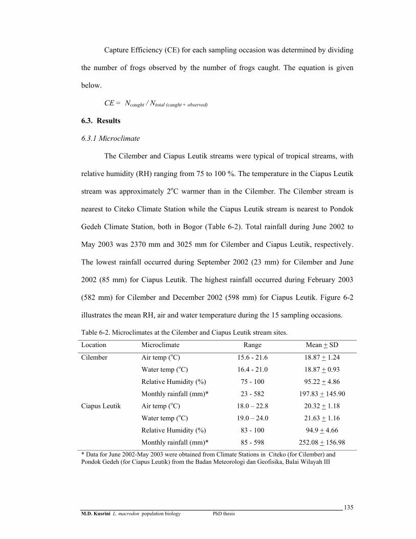
M.D. Kusrini L. macrodon population biology PhD thesis
135
Capture Efficiency (CE) for each sampling occasion was determined by dividing
the number of frogs observed by the number of frogs caught. The equation is given
below.
CE = Ncaught / Ntotal (caught + observed)
6.3. Results
6.3.1 Microclimate
The Cilember and Ciapus Leutik streams were typical of tropical streams, with
relative humidity (RH) ranging from 75 to 100 %. The temperature in the Ciapus Leutik
stream was approximately 2oC warmer than in the Cilember. The Cilember stream is
nearest to Citeko Climate Station while the Ciapus Leutik stream is nearest to Pondok
Gedeh Climate Station, both in Bogor (Table 6-2). Total rainfall during June 2002 to
May 2003 was 2370 mm and 3025 mm for Cilember and Ciapus Leutik, respectively.
The lowest rainfall occurred during September 2002 (23 mm) for Cilember and June
2002 (85 mm) for Ciapus Leutik. The highest rainfall occurred during February 2003
(582 mm) for Cilember and December 2002 (598 mm) for Ciapus Leutik. Figure 6-2
illustrates the mean RH, air and water temperature during the 15 sampling occasions.
Table 6-2. Microclimates at the Cilember and Ciapus Leutik stream sites.
Location Microclimate Range Mean + SD
Cilember Air temp (oC) 15.6 - 21.6 18.87 + 1.24
Water temp (oC) 16.4 - 21.0 18.87 + 0.93
Relative Humidity (%) 75 - 100 95.22 + 4.86
Monthly rainfall (mm)* 23 - 582 197.83 + 145.90
Ciapus Leutik Air temp (oC) 18.0 – 22.8 20.32 + 1.18
Water temp (oC) 19.0 – 24.0 21.63 + 1.16
Relative Humidity (%) 83 - 100 94.9 + 4.66
Monthly rainfall (mm)* 85 - 598 252.08 + 156.98
* Data for June 2002-May 2003 were obtained from Climate Stations in Citeko (for Cilember) and Pondok Gedeh (for Ciapus Leutik) from the Badan Meteorologi dan Geofisika, Balai Wilayah III

M.D. Kusrini L. macrodon population biology PhD thesis
136
6.3.2 Captures
A total of 42 individual L. macrodon were captured a total of 64 times
(including recaptures) at the Cilember stream. Almost three quarters (n = 30) were
captured once, six were captured twice, three were captured three times, two were
captured four times and one was captured five times (Figure 6-3). Thirty-four frogs
were observed but not captured. Mean capture efficiency + SE in the Cilember stream
was 0.71 + 0.06. The greatest numbers were observed in November 2002 (n = 19),
December 2002 (n = 17) and February 2003 (n = 13). The highest density of frogs
observed in a 100 m segment of the transect was 7 individuals on 26 December 2002.
No frogs were observed during August and October 2002, and July 2004 (Figure 6-4).
Fewer frogs were observed and captured at the Ciapus Leutik stream. A total of
20 individuals were captured, 15 of them once, four twice, and one three times (Figure
6-5), for a total of 26 capture occasions. Eighteen frogs were observed but not captured.
Mean capture efficiency + SE at Ciapus Leutik was 0.59 + 0.1. The greatest number of
frogs were observed in April 2003 (n = 6), February 2003, and July 2004 (both n = 4).
Frog density was lower at this stream; the usual density was one or two per 100 m of
transect. No frogs were captured during January 2003 and April 2004, however frogs
were still observed at those times (Figure 6-6).

M.D. Kusrini L. macrodon population biology PhD thesis
137
A. Cilember
0
5
10
15
20
25
Jun-02
Jul-02
Aug-02
Sep-02
Oct-02
Nov-02
Dec-02
Jan-03
Feb-03
Mar-03
Apr-03
May-03
Jan-04
Apr-04
Jul-04
months
tem
pere
atur
e (o
C)
84
86
88
90
92
94
96
98
100
RH
(%)
mean RH (%)mean air temp (oC)mean water temp (oC)
B. Ciapus Leutik
0
5
10
15
20
25
Jun-02
Jul-02
Aug-02
Sep-02
Oct-02
Nov-02
Dec-02
Jan-03
Feb-03
Mar-03
Apr-03
May-03
Jan-04
Apr-04
Jul-04
months
tem
pera
ture
(oC
)
84
86
88
90
92
94
96
98
100
RH
(%)
mean RH (%)
mean air temp (oC)
mean w ater temp (oC)
Figure 6-2. Mean relative humidity (%), air and water temperature (oC) in the Cilember and the
Ciapus Leutik Stream during sampling.
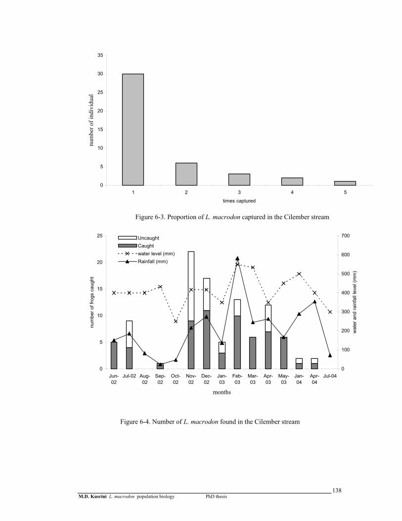
M.D. Kusrini L. macrodon population biology PhD thesis
138
0
5
10
15
20
25
30
35
1 2 3 4 5
times captured
num
ber o
f ind
ivid
ual
Figure 6-3. Proportion of L. macrodon captured in the Cilember stream
0
5
10
15
20
25
Jun-02
Jul-02 Aug-02
Sep-02
Oct-02
Nov-02
Dec-02
Jan-03
Feb-03
Mar-03
Apr-03
May-03
Jan-04
Apr-04
Jul-04
months
num
ber o
f fro
gs c
augh
t
0
100
200
300
400
500
600
700
wat
er a
nd ra
infa
ll le
vel (
mm
)
UncaughtCaughtwater level (mm)Rainfall (mm)
Figure 6-4. Number of L. macrodon found in the Cilember stream
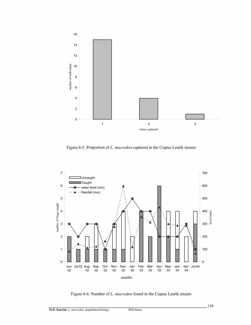
M.D. Kusrini L. macrodon population biology PhD thesis
139
0
2
4
6
8
10
12
14
16
1 2 3
times captured
num
ber o
f ind
ivid
ual
Figure 6-5. Proportion of L. macrodon captured in the Ciapus Leutik stream
0
1
2
3
4
5
6
7
Jun-02
Jul-02 Aug-02
Sep-02
Oct-02
Nov-02
Dec-02
Jan-03
Feb-03
Mar-03
Apr-03
May-03
Jan-04
Apr-04
Jul-04
num
ber o
f fro
gs c
augh
t
0
100
200
300
400
500
600
700
months
leve
l (m
m)
UncaughtCaughtwater level (mm)Rainfall (mm)
Figure 6-6. Number of L. macrodon found in the Ciapus Leutik stream

M.D. Kusrini L. macrodon population biology PhD thesis
140
During the 12-month continuous survey period (June 2002 – May 2003), more
frogs were found during the third and fourth 3-month periods (Figure 6-7), which
coincided with higher rainfall. There is a positive correlation between numbers of frogs
observed and mean monthly rainfall based on these four periods (Cilember r = 0.658, P
= 0.020; Ciapus Leutik r = 0.714, P = 0.009).
Jun - Aug 2002 Sept - Nov 2002 Dec 2002 - Feb 2003 Mar - May 2003
periods
0
5
10
15
20
mea
n nu
mbe
r of f
rogs
foun
d
LocationCilemberCiapus Leutik
Figure 6-7. Mean frogs found (observed and captured) in the Cilember and the Ciapus Leutik
streams during 4-monthly periods in the continuous period between June 2002 and May 2003
6.3.3. Traits of L. macrodon
Including recaptures and frogs encountered but not captured, a total of 142 frogs
were encountered across both sites during the study. L. macrodon was not the most
abundant species at the study sites. Limnonectes kuhlii was the most common species at
Cilember, while Rana hosii was the most common frog at Ciapus Leutik.
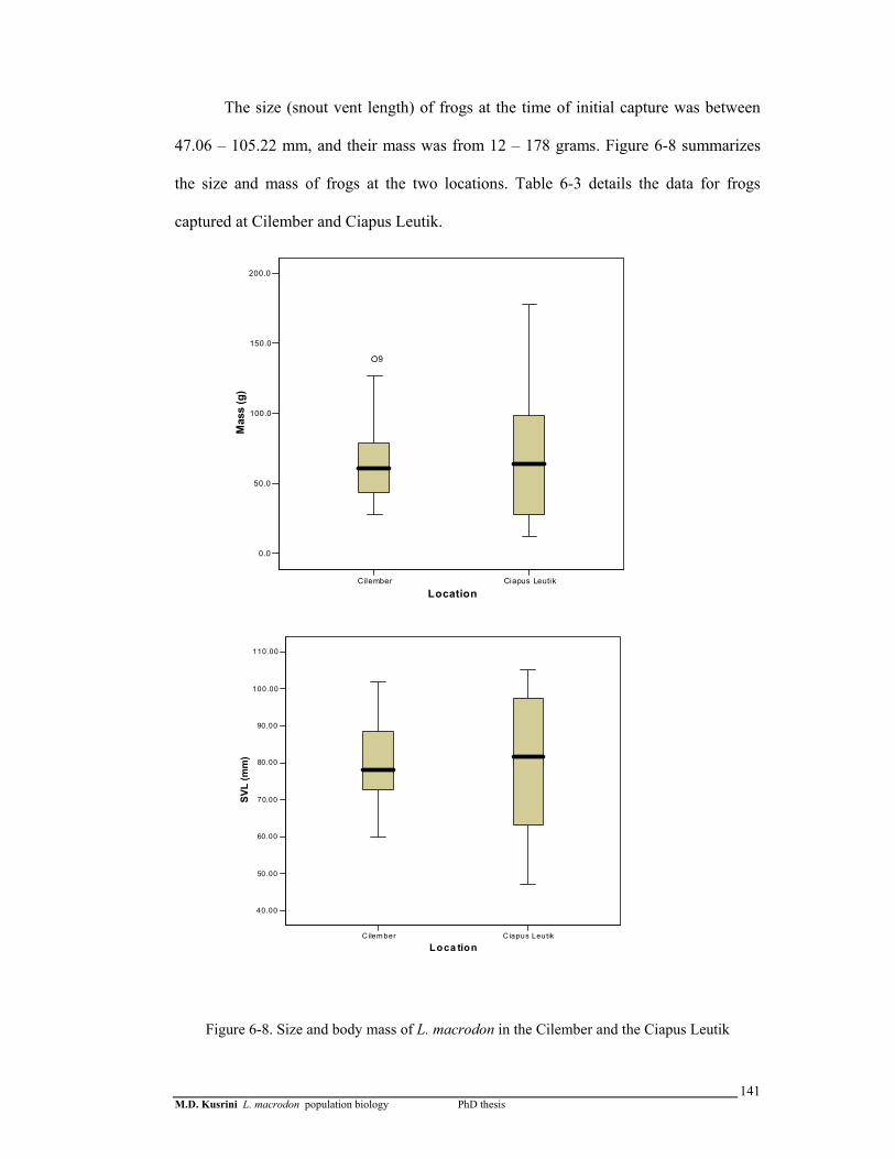
M.D. Kusrini L. macrodon population biology PhD thesis
141
The size (snout vent length) of frogs at the time of initial capture was between
47.06 – 105.22 mm, and their mass was from 12 – 178 grams. Figure 6-8 summarizes
the size and mass of frogs at the two locations. Table 6-3 details the data for frogs
captured at Cilember and Ciapus Leutik.
Cilember Ciapus Leutik
Location
0.0
50.0
100.0
150.0
200.0
Mas
s (g
)
9
C ilem ber C iapus Leutik
Loca tion
40.00
50.00
60.00
70.00
80.00
90.00
100.00
110.00
SVL
(mm
)
Figure 6-8. Size and body mass of L. macrodon in the Cilember and the Ciapus Leutik

M.D. Kusrini L. macrodon population biology PhD thesis
142
Table 6-3. Traits of L. macrodon in the Cilember and Ciapus Leutik streams
SVL (mm) Mass (grams)
Location N Range Mean + SD Range Mean + SD
Cilember 42 60.00 - 101.74 79.67 + 11.52 27.60 - 136.00 65.35 + 29.11
Ciapus Leutik 20 47.06 - 105.22 78.25 + 18.25 12.00 - 178.00 68.41 + 48.59
There were no significant differences between Cilember and Ciapus Leutik in
the mean SVL (F1,60 = 0.14, P =0.71) or mass (F1,60 = 0.09, P =0.76), of frogs.
Log(mass) and log(SVL) were strongly correlated at both sites (Cilember: r = 0.906, N
= 42, P < 0.001; Ciapus Leutik: r = 0.949, N = 20, P < 0.001). These relationships are
shown in Figure 6-9.
1.00 1.20 1.40 1.60 1.80 2.00 2.20 2.40
mass_log
1.70
1.80
1.90
2.00
svl_
log
LocationCilemberCiapus Leutik
R Sq Linear = 0.929
Figure 6-9. Relationship between snout vent length (mm) and mass (gram) of L. macrodon
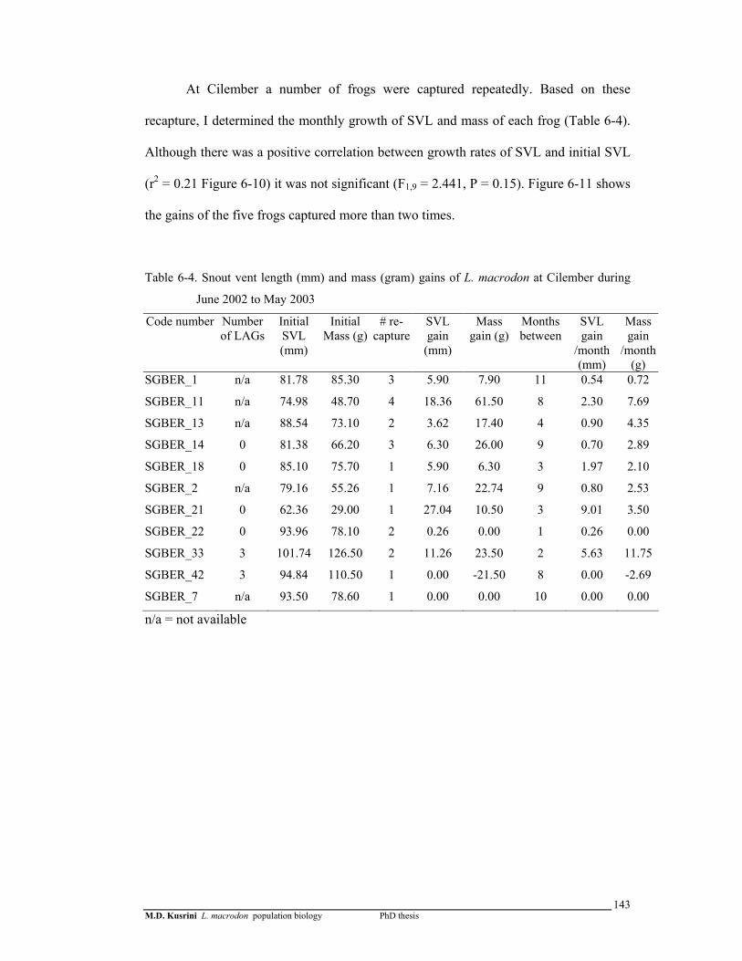
M.D. Kusrini L. macrodon population biology PhD thesis
143
At Cilember a number of frogs were captured repeatedly. Based on these
recapture, I determined the monthly growth of SVL and mass of each frog (Table 6-4).
Although there was a positive correlation between growth rates of SVL and initial SVL
(r2 = 0.21 Figure 6-10) it was not significant (F1,9 = 2.441, P = 0.15). Figure 6-11 shows
the gains of the five frogs captured more than two times.
Table 6-4. Snout vent length (mm) and mass (gram) gains of L. macrodon at Cilember during
June 2002 to May 2003
Code number Number of LAGs
Initial SVL (mm)
Initial Mass (g)
# re-capture
SVL gain (mm)
Mass gain (g)
Months between
SVL gain
/month (mm)
Mass gain
/month (g)
SGBER_1 n/a 81.78 85.30 3 5.90 7.90 11 0.54 0.72
SGBER_11 n/a 74.98 48.70 4 18.36 61.50 8 2.30 7.69
SGBER_13 n/a 88.54 73.10 2 3.62 17.40 4 0.90 4.35
SGBER_14 0 81.38 66.20 3 6.30 26.00 9 0.70 2.89
SGBER_18 0 85.10 75.70 1 5.90 6.30 3 1.97 2.10
SGBER_2 n/a 79.16 55.26 1 7.16 22.74 9 0.80 2.53
SGBER_21 0 62.36 29.00 1 27.04 10.50 3 9.01 3.50
SGBER_22 0 93.96 78.10 2 0.26 0.00 1 0.26 0.00
SGBER_33 3 101.74 126.50 2 11.26 23.50 2 5.63 11.75
SGBER_42 3 94.84 110.50 1 0.00 -21.50 8 0.00 -2.69
SGBER_7 n/a 93.50 78.60 1 0.00 0.00 10 0.00 0.00
n/a = not available

M.D. Kusrini L. macrodon population biology PhD thesis
144
A. SVL (mm)
60
65
70
75
80
85
90
95
100
105
110
115
120
snou
t ven
t len
gth
(mm
)
SGBER 1 SGBER 11SGBER 14 SGBER 13SGBER 33 2 per. Mov. Avg. (SGBER 11)2 per. Mov. Avg. (SGBER 1) 2 per. Mov. Avg. (SGBER 14)
Figure 6-10. SVL and mass gain of five L. macrodon in the Cilember stream. Months 1–12 are
June 2002 to May 2003 respectively. Trendlines are shown only for frogs recaptured more than three times.
B. Mass40
60
80
100
120
140
1600 1 2 3 4 5 6 7 8 9 10 11 12
month
mas
s (g
ram
)
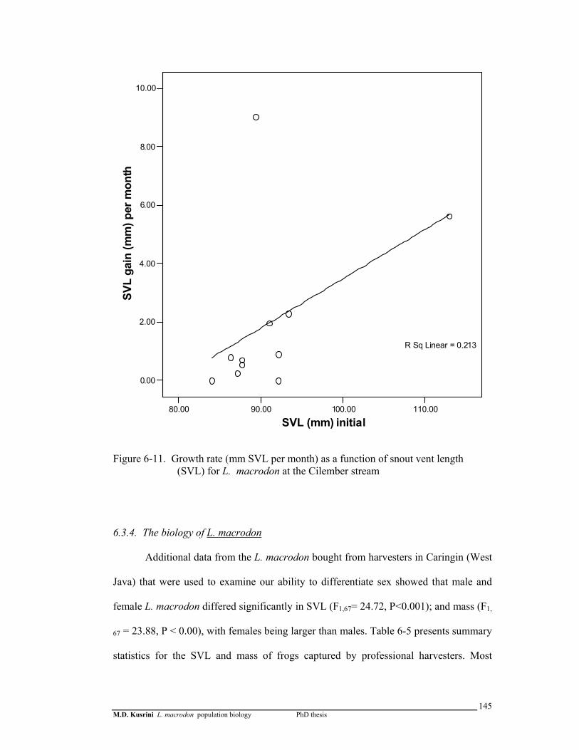
M.D. Kusrini L. macrodon population biology PhD thesis
145
80.00 90.00 100.00 110.00
SVL (mm) initial
0.00
2.00
4.00
6.00
8.00
10.00
SVL
gain
(mm
) per
mon
th
R Sq Linear = 0.213
Figure 6-11. Growth rate (mm SVL per month) as a function of snout vent length
(SVL) for L. macrodon at the Cilember stream
6.3.4. The biology of L. macrodon
Additional data from the L. macrodon bought from harvesters in Caringin (West
Java) that were used to examine our ability to differentiate sex showed that male and
female L. macrodon differed significantly in SVL (F1,67= 24.72, P<0.001); and mass (F1,
67 = 23.88, P < 0.00), with females being larger than males. Table 6-5 presents summary
statistics for the SVL and mass of frogs captured by professional harvesters. Most
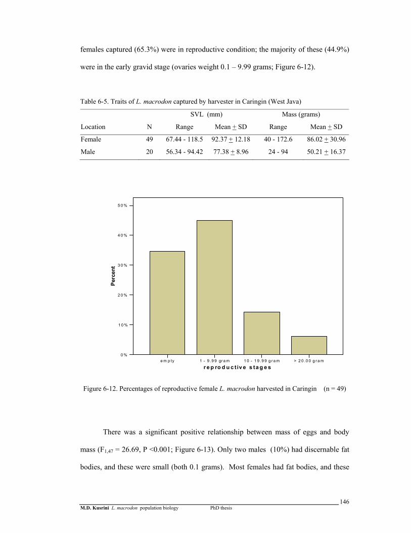
M.D. Kusrini L. macrodon population biology PhD thesis
146
females captured (65.3%) were in reproductive condition; the majority of these (44.9%)
were in the early gravid stage (ovaries weight 0.1 – 9.99 grams; Figure 6-12).
Table 6-5. Traits of L. macrodon captured by harvester in Caringin (West Java)
SVL (mm) Mass (grams)
Location N Range Mean + SD Range Mean + SD
Female 49 67.44 - 118.5 92.37 + 12.18 40 - 172.6 86.02 + 30.96
Male 20 56.34 - 94.42 77.38 + 8.96 24 - 94 50.21 + 16.37
e m p ty 1 - 9 .9 9 gr a m 1 0 - 1 9 .9 9 g r a m > 2 0 .0 0 g r a m
r e p ro d u c t iv e s ta g e s
0 %
1 0 %
2 0 %
3 0 %
4 0 %
5 0 %
Perc
ent
Figure 6-12. Percentages of reproductive female L. macrodon harvested in Caringin (n = 49)
There was a significant positive relationship between mass of eggs and body
mass (F1,47 = 26.69, P <0.001; Figure 6-13). Only two males (10%) had discernable fat
bodies, and these were small (both 0.1 grams). Most females had fat bodies, and these
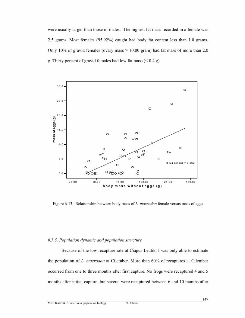
M.D. Kusrini L. macrodon population biology PhD thesis
147
were usually larger than those of males. The highest fat mass recorded in a female was
2.5 grams. Most females (95.92%) caught had body fat content less than 1.0 grams.
Only 10% of gravid females (ovary mass > 10.00 gram) had fat mass of more than 2.0
g. Thirty percent of gravid females had low fat mass (< 0.4 g).
2 5 .0 0 50 .0 0 7 5.0 0 1 0 0 .0 0 1 2 5 .0 0 1 5 0 .0 0
b o d y m a s s w ith o u t e g g s (g )
0 .0
5 .0
1 0 .0
1 5 .0
2 0 .0
2 5 .0
3 0 .0
mas
s of
egg
s (g
)
R S q L in e a r = 0 .36 2
Figure 6-13. Relationship between body mass of L. macrodon female versus mass of eggs
6.3.5. Population dynamic and population structure
Because of the low recapture rate at Ciapus Leutik, I was only able to estimate
the population of L. macrodon at Cilember. More than 60% of recaptures at Cilember
occurred from one to three months after first capture. No frogs were recaptured 4 and 5
months after initial capture, but several were recaptured between 6 and 10 months after
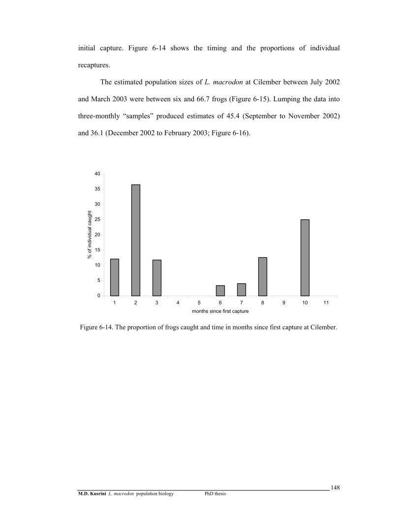
M.D. Kusrini L. macrodon population biology PhD thesis
148
initial capture. Figure 6-14 shows the timing and the proportions of individual
recaptures.
The estimated population sizes of L. macrodon at Cilember between July 2002
and March 2003 were between six and 66.7 frogs (Figure 6-15). Lumping the data into
three-monthly “samples” produced estimates of 45.4 (September to November 2002)
and 36.1 (December 2002 to February 2003; Figure 6-16).
0
5
10
15
20
25
30
35
40
1 2 3 4 5 6 7 8 9 10 11
months since first capture
% o
f ind
ivid
ual c
augh
t
Figure 6-14. The proportion of frogs caught and time in months since first capture at Cilember.
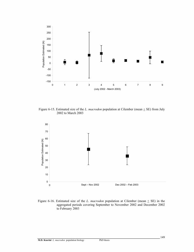
M.D. Kusrini L. macrodon population biology PhD thesis
149
-150
-100
-50
0
50
100
150
200
250
300
0 1 2 3 4 5 6 7 8 9
(July 2002 - March 2003)
Popu
latio
n Es
timat
ed (N
)
Figure 6-15. Estimated size of the L. macrodon population at Cilember (mean + SE) from July 2002 to March 2003
Figure 6-16. Estimated size of the L. macrodon population at Cilember (mean + SE) in the
aggregated periods covering September to November 2002 and December 2002 to February 2003
0
10
20
30
40
50
60
70
80
0 Sept – Nov 2002 Dec 2002 – Feb 2003
Popu
latio
n Es
timat
ed (N
)
0
10
20
30
40
50
60
70
80
0 Sept – Nov 2002 Dec 2002 – Feb 2003
Popu
latio
n Es
timat
ed (N
)
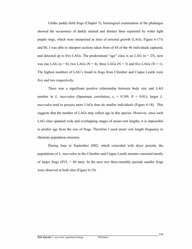
M.D. Kusrini L. macrodon population biology PhD thesis
150
Unlike paddy-field frogs (Chapter 5), histological examination of the phalanges
showed the occurrence of darkly stained and distinct lines separated by wider light
purple rings, which were interpreted as lines of arrested growth (LAGs, Figure 6-17A
and B). I was able to interpret sections taken from of 44 of the 46 individuals captured,
and detected up to five LAGs. The predominant “age” class is no LAG (n = 25), next
was one LAG (n = 8), two LAGs (N = 4), three LAGs (N = 3) and five LAGs (N = 1).
The highest numbers of LAG’s found in frogs from Cilember and Ciapus Leutik were
five and two respectively.
There was a significant positive relationship between body size and LAG
number in L. macrodon (Spearman correlation, rs = 0.399, P = 0.01); larger L.
macrodon tend to possess more LAGs than do smaller individuals (Figure 6-18). This
suggests that the number of LAGs may reflect age in this species. However, since each
LAG class spanned wide and overlapping ranges of snout-vent lengths, it is impossible
to predict age from the size of frogs. Therefore I used snout vent length frequency to
illustrate population structure.
During June to September 2002, which coincided with dryer periods, the
populations of L. macrodon in the Cilember and Ciapus Leutik streams consisted mostly
of larger frogs (SVL > 80 mm). In the next two three-monthly periods smaller frogs
were observed at both sites (Figure 6-19).

M.D. Kusrini L. macrodon population biology PhD thesis
151
Figure 6-17A. Limnonectes macrodon from the Cilember stream with five LAGs; Arrows pointing to LAGs (SVL 77.86 m, mass = 61 g)
Figure 6-17B. Limnonectes macrodon from the Cilember stream with three LAGs; Arrows
pointing to LAGs (SVL 101.74 mm, mass = 126.5 g)

M.D. Kusrini L. macrodon population biology PhD thesis
152
0 1 2 3 4 5
Number of LAGs
40
50
60
70
80
90
100
110
SVL(
mm
)
R Sq Linear = 0.139
Figure 6-18. Snout vent length (mm) versus number of lines of arrested growth (LAGs) for Limnonectes macrodon
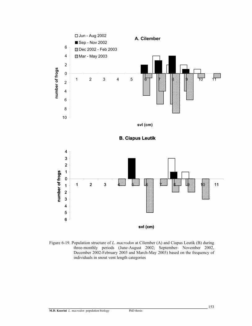
M.D. Kusrini L. macrodon population biology PhD thesis
153
A. Cilember
10
8
6
4
2
0
2
4
6
1 2 3 4 5 6 7 8 9 10 11
svl (cm)
num
ber o
f fro
gs
Jun - Aug 2002Sep - Nov 2002Dec 2002 - Feb 2003Mar - May 2003
A. Cilember
10
8
6
4
2
0
2
4
6
1 2 3 4 5 6 7 8 9 10 11
svl (cm)
num
ber o
f fro
gs
Jun - Aug 2002Sep - Nov 2002Dec 2002 - Feb 2003Mar - May 2003
Figure 6-19. Population structure of L. macrodon at Cilember (A) and Ciapus Leutik (B) during
three-monthly periods (June-August 2002; September- November 2002, December 2002-February 2003 and March-May 2003) based on the frequency of individuals in snout vent length categories
B. Ciapus Leutik
65432101234
1 2 3 4 5 6 7 8 9 10 11
svl (cm)
num
ber o
f fro
gs
B. Ciapus Leutik
65432101234
1 2 3 4 5 6 7 8 9 10 11
svl (cm)
num
ber o
f fro
gs

M.D. Kusrini L. macrodon population biology PhD thesis
154
6.3.6 Microhabitat use
At Cilember most L. macrodon were found in the lower 200 m of the transect.
Although four frogs were captured and marked in the upper 200 m of the transect, all
recaptures were from the lower 200 m. L. macrodon at Ciapus Leutik were all found in
the 0 – 100 m and 200 – 350 m regions of the transect (Figure 6-20).
0 100 200 300
position along transect (m)
0
3
6
9
12
15
mon
th
markedobserved
0 100 200 300 400
position along transect (m)
0
3
6
9
12
15
mon
th
Figure 6-20. The positions of L. macrodon along the transects in the Cilember stream (left) and
the Ciapus Leutik stream (right). Months 1 – 12 are June 2002 to May 2003. Month 13 = January 2004, month 14 = April 2004, month 15 = July 2004. No L. macrodon were found in month 15 in the Cilember stream.
Most frogs were found in relatively protected locations such as holes or rock
crevices where they mostly sat quietly (Figure 6-21). Some were found in open areas
such as grassy banks, or were swimming in the water. However, most frogs found in
open areas were usually quick to jump and swim away and were therefore difficult to
catch.
6.3.7 Movement
Movement results are presented only for Cilember. The number of frogs
recaptured at Ciapus Leutik was too low for meaningful estimation of movement
parameters. The mean cumulative distance moved per month was 11.41 m (Table 6-6).

M.D. Kusrini L. macrodon population biology PhD thesis
155
Of the 21 movements recorded, two-thirds were ten metres or less. The longest
movements were two mean monthly movements of 60 m, which happened within the
span of one (October to November 2002) and two months (March to May 2003).
Figure 6-21. The percentage of L. macrodon found in four types of microhabitat
Table 6-6. Summary of movement of L. macrodon at the Cilember stream
Distance movement per month (m)
Displacement per month **
Straightness**
Mean + SD 11.41 + 17.25 5.75 + 4.61 0.6 + 0.32
Range 0.33 - 60 0.33 – 11.75 0.29 – 1.00
** only for frogs recaptured more than once
o n s o il i n p r o t e c t e d h o l e s
ro c k c r e v ic e s g r a s s y b a n k w a t e r
m ic ro h a b i t a t
0 %
1 0 %
2 0 %
3 0 %
4 0 %
5 0 %
6 0 %
7 0 %
Perc
ent f
rog
foun
d
C i le m b e rC i a p u s L e u t i k
M.D. Kusrini L. macrodon population biology PhD thesis
156
6.4 Discussion
Mean SVL for L. macrodon in this study was 79.21 mm (range 47.06 – 113 mm)
and mean mass was 66.34 grams (range 12 – 178 grams). The largest frogs captured in
this study were 113 mm in SVL (mass = 110 grams) and 178 grams in mass (SVL =
105.22 mm). Most frogs captured were less than 80 mm SVL, which is the modal size
captured by professional harvesters. The maximum sizes of frogs found in this study are
less than the maximum sizes of frogs captured by harvesters in previous years. For
instance, based on Sugiri (1979), the biggest L. macrodon captured by harvesters in
West Java was 209.8 g (male, SVL = 119 mm, captured September 1975) and 214.0 g
(female, SVL = 121 mm, captured in May 1976). The latter also had the longest SVL
for female, whilst for a male the largest SVL was 144 mm (mass 109.4 g, captured in
August 1976).
Recaptures at Cilember showed that most individuals were growing relatively
rapidly. Growth in frogs is usually rapid when they are small but slows towards an
asymptote when frogs mature (Ramirez et al., 1998). In my data, one individual with an
SVL of more than 100 mm was growing more rapidly than some smaller individuals,
suggesting that rapid growth can continue past reproductive size in at least some
individuals.
Most work on fanged frogs indicates that adult males are larger than females
(Inger, 1966; Emerson and Ward, 1998), however this study found the opposite result.
The sex of individuals in my field study was very uncertain due to the difficulty of
sexing individuals, however additional data from L. macrodon bought from harvesters
in Caringin (West Java) that was used to differentiate sex indicated that females were on
average larger than males. Sugiri (1978) concluded that there were no significant
differences in mass or SVL between male and female L. macrodon from West Java.

M.D. Kusrini L. macrodon population biology PhD thesis
157
Both Sugiri’s (1979) and my study found that professional harvesters captured more
females, which is the same trend as that for Fejervarya cancrivora (Chapter 3), in which
females are larger than males. These results suggest that L. macrodon exhibits a pattern
of sexual dimorphism different from that of other fanged species. Since both Sugiri’s
and my data were derived from professional harvesters, they may reflect biases in
collection. Large female L. macrodon could be easier to catch than large males,
possibly because most females captured by professional harvesters were gravid; males
may also be more wary. As with other species of frogs, mating of fanged frogs such as
L. blythi involves an active movement of gravid females to search for suitable adult
males (Emerson and Inger, 1992)
Sugiri (1979) found that the smallest female with ovaries in the early gravid
stage (ovaries weight ca. 2.1 g) was 72 mm SVL and weighed 50.1 g. In my study the
smallest female frog that had ovaries in this stage was 67.44 mm and weighed 40 g.
This suggests that the minimum reproductive size for female L. macrodon is probably
around 60 to 65 mm SVL.
My results show that skeletochronology may be applicable to L. macrodon.
LAGs found in L. macrodon were quite distinct, suggesting that growth was slower
during certain times, most probably during the dry season, which only occurs for around
three months each year. Compared to the rice field frogs, L. macrodon tends to be
philopatric, remaining in sites during the dry season. In temperate species, LAGs are
usually visible, and are formed during winter (Halliday and Verrel 1988; Ryser 1988;
Reaser 2000). Results from this study confirmed the findings of Felton (1999), and
Kumbar and Pancharatna (2001) that skeletochronology can be used to determine the
ages of tropical frogs.

M.D. Kusrini L. macrodon population biology PhD thesis
158
Because I found a relatively large number of L. macrodon individuals with more
than a single LAG, but found only zero or one LAGs in F. limnocharis-iskandari
complex and F. cancrivora, it is possible that L. macrodon may be longer-lived than
either of these species. However, further study is required to validate that LAGs are
formed annually in L. macrodon and the other species. Although it seems likely that
increasing numbers of LAGs indicates increasing age in L. macrodon, the exact
relationship between LAG number and age is not clear from my results. Number of
LAGs and SVL are correlated, but each LAG class spans a wide and overlapping range
of snout-vent lengths. Also, because frogs were not recaptured and clipped a second
time for reanalysis after one year, there is no direct evidence that LAGs are formed
annually. Therefore, there is a need to validate the relationship between LAGs and age,
ideally by re-clipping recaptured frogs.
The lower limit of snout vent length for LAG-1 in this study was 62.88 mm, and
for the early reproductive stages of females was 67.44 mm. These figures suggest that
mature L. macrodon have a SVL of at least 60 mm, which may be attained at
approximately one year of age. The populations of L. macrodon at Cilember and Ciapus
Leutik consisted mainly of adult individuals. I did not find any tadpoles during the
study, nor did I observe reproductive activity. However, some frogs were found sitting
near pool-like areas on the edge of the streams near the banks (Figure 6-22) that would
be suitable habitat for breeding not only for L. macrodon (Iskandar, 1998) but also for
other Limnonectes species such as L. kuhlii (Tsuji and Lue, 2000) and L. blythi
(Emerson, 1992).

M.D. Kusrini L. macrodon population biology PhD thesis
159
Figure 6-22. Pool-like area in the Ciapus Leutik stream where L. macrodon was sometimes
found
Monthly population estimates either could not be calculated using Jolly Seber
method, or had relatively high standard errors. The number of individuals captured at
Ciapus Leutik was so low that monthly population estimation was impossible, and
monthly population estimates at Cilember varied greatly (Figure 6-14). Estimates using
the Jolly-Seber technique on data aggregated into three-monthly periods were more
reliable, with smaller standard errors. It seems likely that variation in capture
probabilities play a factor in the variability of population estimation. It is likely that
capture probability is not constant, but is affected by seasonal factors and short-term
effects on frog behaviour. For example, it appeared that more frogs were active during
higher rainfall periods (Figure 6-7).
Capture efficiency also could affect population estimates; at Cilember and
Ciapus Leutik it varied between 0.59 and 0.71, which means for every two to three
frogs captured, one frog escaped. Limnonectes macrodon were rarely found in open
M.D. Kusrini L. macrodon population biology PhD thesis
160
areas, most were found in protected microhabitats, which made them harder to find. The
frogs were also very agile and had a tendency to escape during capture and handling.
After initial capture, the probability of recapture might decrease. Probability of capture
also differs between individuals in the population, which explained why some
individuals could only be recaptured more than six months after their initial capture,
while most were recaptured between one to three months after initial capture. Frogs also
moved upstream and downstream, although movement seemed restricted by natural
boundaries, such as the occurrence of waterfalls, most notably at Cilember. The
movements of L. macrodon at Cilember were probably related to selection of sites
needed for specific activities, such as breeding and foraging. Site selection could change
over time, which might explain why some frogs move more further than others.
Frogs were found in lower numbers at Ciapus Leutik than at Cilember. These
apparent differences in population density could have been caused by differences in
factors such as microclimate, food availability and predation rates (Duellman and
Trueb, 1994). No data are available regarding food availability at the sites, however it
is likely that microclimate and prey abundance in both locations were relatively similar.
Risk of predation is presumably higher from human hunting than from natural predators
such as snakes. As mentioned before, the survey area at Cilember falls within the
boundary of Perum Perhutani recreation area where access is restricted to paid visitors.
Because frog harvesters tend to keep costs low by capturing frogs in unrestricted areas
(Chapter 3), there is no known professional harvesting at the Cilember stream.
However, there is always a possibility that professional or amateur harvesters could
catch frogs that moved outside the fenced area. We found no professional harvesters
during our surveys at Ciapus Leutik, nevertheless some frog harvesters mentioned this
area as one of their regular places to capture frogs. Although there was no significant
M.D. Kusrini L. macrodon population biology PhD thesis
161
difference between mean SVL and mass of frog between Cilember and Ciapus Leutik,
skeletochronological evidence suggests that the Cilember population includes more
older frogs than Ciapus Leutik. This, and the low density of frogs at Ciapus Leutik,
could be related to its greater accessibility to frog harvesters. However, further
monitoring is needed before it is possible to draw any conclusions regarding whether
over-harvesting is the cause of low numbers of frogs at the Ciapus Leutik stream.
M.D. Kusrini Environment stress PhD thesis
161
CHAPTER 7
EFFECTS OF ENVIRONMENTAL STRESS
7.1 Introduction
The population dynamics of amphibians depend on the quality of the
environments they occupy. Stress in the environment caused by natural factors such as
climate change or human-induced factors such as chemical contaminants could directly
or indirectly affect the dynamics and status of populations. Many scientists believe that
amphibians are at high risk from contaminants and other stress effects that could
interact with other factors (Alford and Richards, 1999), and which have resulted in
several reported amphibian population declines across the world during the past 15
years (Barinaga, 1990; Blaustein and Wake, 1990; Anonymous, 1991; Pechman et al.,
1991; Tyler, 1991; Blaustein, 1994; Blaustein et al., 1994; Pechman and Wilbur, 1994;
Blaustein and Wake, 1995).
Many scientists have suggested that their environmental sensitivity should make
amphibians as good indicators of environmental quality; this idea has been reviewed
thoroughly by Sparling et al. (2000). It is clear that the habitats and ecology of
amphibians make them susceptible to environmental stressors such as contaminants and
diseases. For example, amphibians that live in agricultural fields are at risk from
exposure to chemicals in pesticides or fertilizers (Ouellet et al., 1997; Jocelyn, 1999).
Because of their life cycles (Duellman and Trueb, 1998) amphibians can be exposed to
multiple risks as they pass through different life stages.
Amphibians have developed various adaptations and tolerances to
environmental stressors. For instance, to avoid water loss amphibians can alter their
behaviour through hibernation or looking for shade, or can reduce the surface area
M.D. Kusrini Environment stress PhD thesis
162
exposed to the air to reduce evaporative water loss (Duellman and Trueb, 1986).
Tolerances to environmental stressors have been investigated in Fejervarya cancrivora.
Tadpoles of this species can tolerate water temperatures up to 40oC and salinity up to
40% of sea water, and survive at rates greater than 50% in 80% sea water (Dunson,
1977). Although adaptations like these can reduce the risk to amphibians from natural
environmental stressors, changes in the level of their exposure to these stressors could
still produce increased physiological stress, slowing the development and growth rate of
juveniles and increasing the vulnerability of frogs to disease (Carey and Bryant, 1995;
Taylor et al., 1999).
Concerns about environmental stressors are usually related to human-induced
stressors. Pesticides have been applied to agricultural land in developing countries for
decades; this has been perceived either as an advantage because it can increase crop
production, or as a source of problems in environmental health (Igbedioh, 1991;
Ecobichon, 2001). Rice fields or sawah are an important agricultural landscape in
Indonesia. They have been subjected to intensive pesticide use, mostly subsidised and
encouraged by the government. The need to increase rice productivity by combating
pests has led to the application of high levels of pesticides to rice fields. Fox (1993),
Van der Eng (1994) and Settle et al. (1999) describe the background of pesticide use in
Indonesia; highlighting the fact that excess use of insecticides has produced more
insecticide-resistant pests.
Pesticides have been implicated as one of the reasons for amphibian problems
around the world. The impact of pesticides on frogs has been documented by many
authors (Cooke, 1970, 1973, 1977, 1981; Brooks, 1981; Mohanti-Hejmadi and Dutta,
1981; Osborn and French, 1981; Berrill, et al., 1998; Boone and Semlitsch, 2001; and
Relyea and Mills, 2001). In addition to their direct toxic and teratogenic effects, stresses
M.D. Kusrini Environment stress PhD thesis
163
caused by environmental toxicants can increase frogs’ susceptibility to diseases (Carey
and Bryant, 1995; Taylor et al., 1999; Thieman, 2000).
As with other wildlife, frogs are also exposed to various pathogens. Disease in
amphibians has recently become a centre of attention, with intensive investigation of
emerging diseases like chytridiomycosis and ranaviral disease that are linked to frog
population declines (Berger et al., 1998; Daszak et al., 1999). Amphibian
chytridiomycosis is a fatal disease caused by the fungus Batrachochytrium
dendrobatidis (Berger, et al., 1999).
Although amphibian deformities are considered a separate problem to global
amphibian declines (Cohen, 2001), alarm has been raised by the finding of increased
morphological abnormalities, especially in North America (Ouellet, et al., 1997; Helgen
et al, 1998; Meteyer et al., 2000). Pesticides have been suggested as one of the causes of
deformities found in frogs around the world (Ouelett, et al., 1997; Helgen et al., 1998)
although recent evidence suggests that parasites are probably responsible for many
amphibian deformities (Kaiser, 1999; Leong , 2001).
Pesticide residue research has been undertaken for some frogs in agricultural
areas in various parts of the world (Gilliland et al., 2001), however there are no reports
on levels of pesticide residues in Indonesian frogs. There also are no reports on the
occurrence of diseases such as chytridiomycosis in Indonesian frogs.
Developmental Stability Analysis (DSA) is a method that has been used to
detect stress in various species from mammals to insects (Soule and Baker, 1968;
Pankakoski, 1985; Clarke, 1994; Tsubaki, Y. 1998). The most common methods for
measuring and analysing developmental stability involve measurements of fluctuating
asymmetry (FA; Palmer and Strobeck, 1986; Alford, et al., 1999). FA is defined only at
the population level; it is a measure of the extent and frequency of random departures

M.D. Kusrini Environment stress PhD thesis
164
from perfect bilateral symmetry in normally symmetrical structures. The aim of this
study was to investigate the nature of environmental stresses on frogs, focusing on rice
field frogs, by 1) documenting the occurrence and frequency of morphological
anomalies, 2) analysing levels of pesticide residues in water, soil and in the bodies of F.
limnocharis-iskandari complex and F. cancrivora found in rice fields, 3) measuring
levels of fluctuating asymmetry in F. limnocharis-iskandari complex and F. cancrivora
for comparison among populations potentially subjected to different levels of stress, and
4) investigating whether amphibian chytridiomycosis occurs in three species of frogs
(F. limnocharis-iskandari complex , F. cancrivora, and L. macrodon) in West Java.
7. 2. Methods
7.2.1. Study area
The research sites are located in West Java province (see Chapter 4 for full site
descriptions). Samples for pesticide analyses and frogs measured for DSA were taken
from six paddy fields: Caringin, Darmaga, Karawang P (Pesticide), Karawang NP (Non
pesticide), Subang P and Subang NP; these are the locations where populations of F.
limnocharis-iskandari complex and F. cancrivora were studied (Chapter 5). Toe-clips
taken during the population studies at the paddy field sites and at two stream sites
(Cilember and Ciapus Leutik, Chapter 6) were analysed histologically for diagnosis of
chytridiomycosis.
7.2.2 Morphological abnormalities
While doing preliminary surveys with harvesters in Caringin, I noted that
several individuals captured showed morphological abnormalities. I decided to record
any morphological abnormalities found in each individual captured during my
M.D. Kusrini Environment stress PhD thesis
165
population study (Chapter 5). Morphological abnormalities were described and
categorised using terms adapted from Tyler (1999), Meteyer et al. (2000), and Johnson
et al. (2001). I also present preliminary data taken from harvested frogs captured by frog
hunters in Caringin (Bogor) during 2001 and 2002, data from Ciptarasa, Panguyangan
and Cisaat taken from 2001 preliminary surveys, and data from specimens located in the
Museum Zoology Bogor (MZB) in Cibinong, Bogor, Indonesia.
Site prevalence for each species is calculated as (number of abnormal
individuals)/(total number of individuals) X 100. I used chi-squared homogeneity tests
for each species to examine possible differences in the proportions of normal and
abnormal frogs among sites. I excluded locations in which less than 20 frogs were found
from this analysis.
7.2.3. Pesticide analysis in rice fields
a. Sample collection
Water, soil, and frog samples were obtained during the harvest season in
September 2002. Water was collected and put into glass bottles and soil samples were
taken using a grab and put inside plastic bags. Three samples of soil and water were
taken from each location and combined for analysis. Three Fejervarya limnocharis-
iskandari complex and three F. cancrivora were taken from each of the six rice fields
using hand collection. No F. cancrivora were found in Darmaga during the sampling
period, therefore samples of this species were only taken from the five other locations.
Snout vent length, mass and sex of each frog were recorded after collection (Table 7-1).
Frogs were brought alive to the Toxicology Laboratory in Bogor. They were
then euthanized and liver and leg muscle tissue was removed for analysis. All sampling

M.D. Kusrini Environment stress PhD thesis
166
and laboratory analyses were undertaken according to an Animal Ethics permit (A 748)
granted by the James Cook University Animal Ethics Sub-Committee.
Table 7-1. Data on individual frogs analysed for pesticide residues in 6 rice fields
F. limnocharis-iskandari complex
F. cancrivora Origin
Sex SVL (mm) Mass (g) Sex SVL (mm) Mass (g) F 50.40 13.00 F 80.20 37.40 F 44.50 10.20 F 60.40 20.80
Caringin
F 45.50 11.60 M 50.60 9.40 F 51.84 11.3 n/a n/a n/a M 48.12 9 n/a n/a n/a
Darmaga
M 49.56 8.9 n/a n/a n/a F 37.46 4.4 F 65.84 26.4 F 30.53 2 M 62.92 22.2
Kawarang NP
F 35.74 3.55 F 59.55 17 M 51.16 9.85 F 55.98 16.20 M 39.33 4.3 J 22.88 1.6
Karawang P
F 28.22 2.6 M 51.16 9.85 F 49.12 n/a M 49.07 12 F 41.23 5.5 M 64.02 27.30
Subang NP
M 46.31 8.4 F 38.37 6.50 F 36.72 4.5 F 50.92 9.5 F 41.22 4.65 F 41.84 5.60
Subang P
F 34.72 3.70 M 33.54 3.95 n/a: Not applicable
b. Pesticide residue analysis
Pesticide residue levels in the liver and leg muscles of frogs were analysed at
the Toxicology Laboratory, Agriculture Biotechnology and Genetic Research Institute
(ABIOGRI), Bogor, West Java, Indonesia using Gas Chromatography (GC) and High
Pressure Liquid Chromatography (HPLC). Pesticide residue analyses used the standard
methods approved by the Indonesian Pesticide Commission (1997), which include (1)
field sampling (2) sample preparation, (3) sample extraction and (4) pesticide residue
analysis. Detection limits based on parts per million (ppm) for each residue using this
method were as follows: BHC (0.001 ppm), aldrin (0.0068 ppm), heptachlor (0.0006
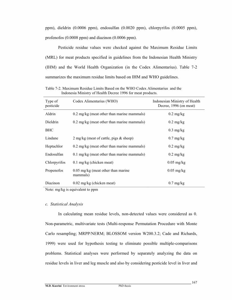
M.D. Kusrini Environment stress PhD thesis
167
ppm), dieldrin (0.0006 ppm), endosulfan (0.0020 ppm), chlorpyrifos (0.0005 ppm),
profenofos (0.0008 ppm) and diazinon (0.0006 ppm).
Pesticide residue values were checked against the Maximum Residue Limits
(MRL) for meat products specified in guidelines from the Indonesian Health Ministry
(IHM) and the World Health Organization (in the Codex Alimentarius). Table 7-2
summarizes the maximum residue limits based on IHM and WHO guidelines.
Table 7-2. Maximum Residue Limits Based on the WHO Codex Alimentarius and the Indonesia Ministry of Health Decree 1996 for meat products.
Type of pesticide
Codex Alimentarius (WHO) Indonesian Ministry of Health Decree, 1996 (on meat)
Aldrin 0.2 mg/kg (meat other than marine mammals) 0.2 mg/kg
Dieldrin 0.2 mg/kg (meat other than marine mammals) 0.2 mg/kg
BHC 0.3 mg/kg
Lindane 2 mg/kg (meat of cattle, pigs & sheep) 0.7 mg/kg
Heptachlor 0.2 mg/kg (meat other than marine mammals) 0.2 mg/kg
Endosulfan 0.1 mg/kg (meat other than marine mammals) 0.2 mg/kg
Chlorpyrifos 0.1 mg/kg (chicken meat) 0.05 mg/kg
Propenofos 0.05 mg/kg (meat other than marine mammals)
0.05 mg/kg
Diazinon 0.02 mg/kg (chicken meat) 0.7 mg/kg
Note: mg/kg is equivalent to ppm
c. Statistical Analysis
In calculating mean residue levels, non-detected values were considered as 0.
Non-parametric, multivariate tests (Multi-response Permutation Procedure with Monte
Carlo resampling; MRPP/NERM; BLOSSOM version W200.3.2; Cade and Richards,
1999) were used for hypothesis testing to eliminate possible multiple-comparisons
problems. Statistical analyses were performed by separately analyzing the data on
residue levels in liver and leg muscle and also by considering pesticide level in liver and
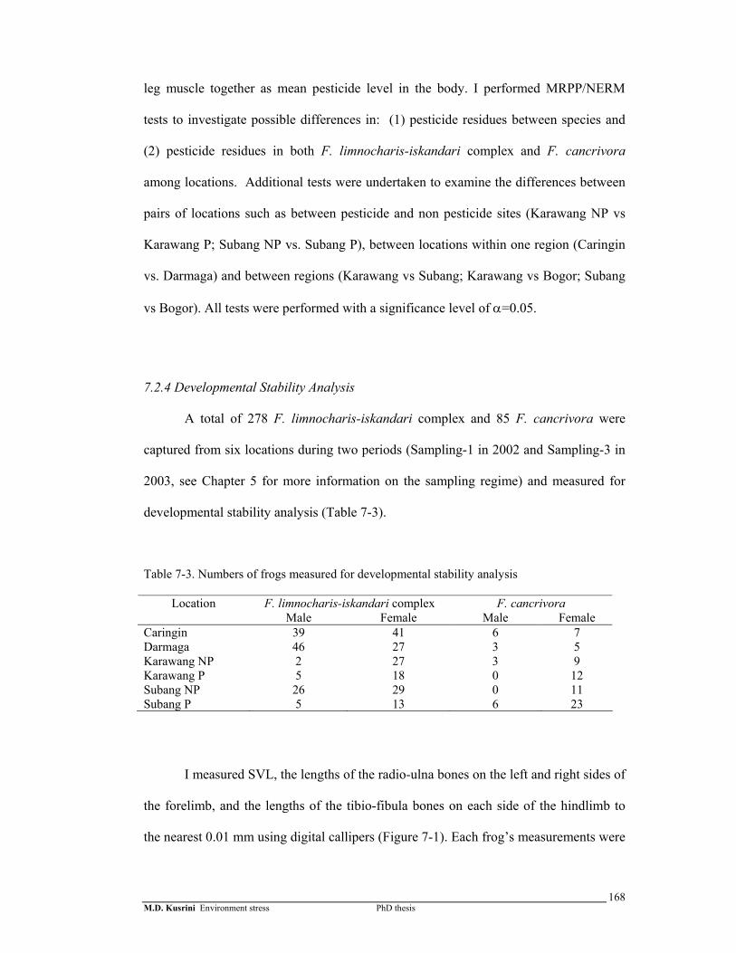
M.D. Kusrini Environment stress PhD thesis
168
leg muscle together as mean pesticide level in the body. I performed MRPP/NERM
tests to investigate possible differences in: (1) pesticide residues between species and
(2) pesticide residues in both F. limnocharis-iskandari complex and F. cancrivora
among locations. Additional tests were undertaken to examine the differences between
pairs of locations such as between pesticide and non pesticide sites (Karawang NP vs
Karawang P; Subang NP vs. Subang P), between locations within one region (Caringin
vs. Darmaga) and between regions (Karawang vs Subang; Karawang vs Bogor; Subang
vs Bogor). All tests were performed with a significance level of α=0.05.
7.2.4 Developmental Stability Analysis
A total of 278 F. limnocharis-iskandari complex and 85 F. cancrivora were
captured from six locations during two periods (Sampling-1 in 2002 and Sampling-3 in
2003, see Chapter 5 for more information on the sampling regime) and measured for
developmental stability analysis (Table 7-3).
Table 7-3. Numbers of frogs measured for developmental stability analysis
F. limnocharis-iskandari complex F. cancrivora Location Male Female Male Female
Caringin 39 41 6 7 Darmaga 46 27 3 5 Karawang NP 2 27 3 9 Karawang P 5 18 0 12 Subang NP 26 29 0 11 Subang P 5 13 6 23
I measured SVL, the lengths of the radio-ulna bones on the left and right sides of
the forelimb, and the lengths of the tibio-fibula bones on each side of the hindlimb to
the nearest 0.01 mm using digital callipers (Figure 7-1). Each frog’s measurements were

M.D. Kusrini Environment stress PhD thesis
169
taken three times, and individuals were remeasured in random sequence. This
measurement protocol was based on that suggested by Alford et al. (1999). The data
were then analysed using a program in SAS (version 6.11) that summarises the
difference between right to left measurements of each character (R-L) and calculates
tests for directional symmetry, anti symmetry, measurement errors and fluctuating
asymmetry based on Palmer and Strobeck (2003).
Figure 7-1. Measurement of hind limb and front limb characters of F. limnocharis-
iskandari complex and F. cancrivora
To remove size effects (Palmer and Strobeck, 2003), data for F. limnocharis-
iskandari complex were transformed by taking their logarithms and reanalysed.
Differences between sexes and among sites were tested for using F-tests on levels of
unsigned (absolute value) asymmetry measured for individuals. If unequal variance
was detected, non-parametric tests were used instead.
To determine whether asymmetry was related to a more conventional measure of
fitness, an index of body condition was calculated for each individual. The index used
Hind limb measurement
Front limb measurement
M.D. Kusrini Environment stress PhD thesis
170
was the residuals from a regression of mass on snout vent length (Dyson et al., 1998).
This was tested for correlation with individual values of unsigned asymmetry using
Spearman rank correlation, which does not require the assumption that any relationship
is linear, only that it is monotonic.
Body condition was also tested for differences between sites and sampling times
using data from population study sampling-1 and sampling-2 (Chapter 5) which were
taken at the same time as the measurements of fluctuating asymmetry. Whenever
possible, these tests were done using ANOVA. When sets of sites or sampling times
had unequal variances, tests were performed nonparametrically using Mann–Whitney
U-tests or Kruskal-Wallis tests.
7.2.5 Chytridiomycosis
Diagnostic histology was undertaken on phalanges taken from toe clips of 103
F. limnocharis-iskandari complex, 35 F. cancrivora and 46 L. macrodon. The
histological examinations were run simultaneously with the skeletochronological
analysis detailed in Chapters 5 and 6, using the same samples. Clipped toes of frogs
taken during field surveys were stored in 4% formalin solution. Each toe was wrapped
in sponge and placed individually in a cassette, then decalcified overnight in 10%
formic acid solution. Toes were then embedded in wax and cut into 10µm sections.
Sections were put on slides and kept in a warming oven at least overnight. The slides
were then put in water and stained with Erlich’s haematoxylin for 20 minutes followed
by two washes in water and two minutes in Scott’s tap water substitute; they were then
mounted with DPX glue. Sections were examined for the presence of amphibian chytrid
zoosporangia in the outer keratin layer using standard diagnostic techniques (Berger et
al., 2000).
M.D. Kusrini Environment stress PhD thesis
171
7.3 Results
7.3.1 Morphological abnormalities
I examined a total of 4331 frogs of 23 species from two habitats (paddy fields
and streams) and found 20 types of deformities. I divided deformities into two general
types: developmental abnormalities and trauma abnormalities (injuries). I distinguished
trauma abnormalities based on the appearance of old scars or, if they involved digits,
the occurrence of digital re-growth. Developmental abnormalities occurred in limbs
(amelia, micromelia, brachymelia, hemimelia, ectromelia, taumelia, cutaneous fusions),
digits (ectrodactyly, brachydactyly, syndactyly, polydactyly, clinodactyly), the back-
bone (scoliosis), the eyes (anophthalmy) and the skin (a lump-like tumor). Trauma
included digit amputation, limb amputation, limb fractured, lip wounds and skin
wounds. Table 7-4 shows the types of abnormalities found, whilst Figure 7-2 shows
several deformities in frogs.
A preliminary survey in Caringin during 2001 and 2002 found abnormalities in
frogs caught by professional hunters. During my first survey in September 2001 I only
noted the number of frogs with abnormalities, I did not note types of abnormalities
(Table 7-5).
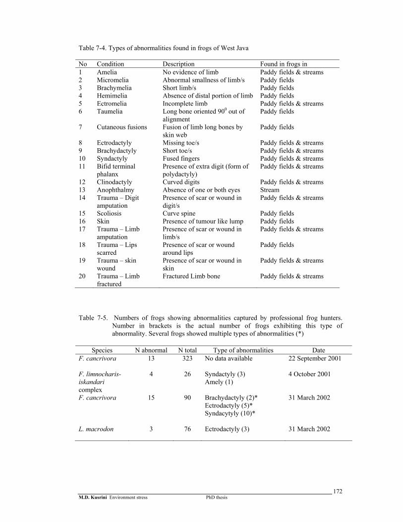
M.D. Kusrini Environment stress PhD thesis
172
Table 7-4. Types of abnormalities found in frogs of West Java
No Condition Description Found in frogs in 1 Amelia No evidence of limb Paddy fields & streams 2 Micromelia Abnormal smallness of limb/s Paddy fields 3 Brachymelia Short limb/s Paddy fields 4 Hemimelia Absence of distal portion of limb Paddy fields 5 Ectromelia Incomplete limb Paddy fields & streams 6
Taumelia Long bone oriented 900 out of alignment
Paddy fields
7 Cutaneous fusions Fusion of limb long bones by skin web
Paddy fields
8 Ectrodactyly Missing toe/s Paddy fields & streams 9 Brachydactyly Short toe/s Paddy fields & streams 10 Syndactyly Fused fingers Paddy fields & streams 11 Bifid terminal
phalanx Presence of extra digit (form of polydactyly)
Paddy fields & streams
12 Clinodactyly Curved digits Paddy fields & streams 13 Anophthalmy Absence of one or both eyes Stream 14 Trauma – Digit
amputation Presence of scar or wound in digit/s
Paddy fields & streams
15 Scoliosis Curve spine Paddy fields 16 Skin Presence of tumour like lump Paddy fields 17 Trauma – Limb
amputation Presence of scar or wound in limb/s
Paddy fields & streams
18 Trauma – Lips scarred
Presence of scar or wound around lips
Paddy fields
19 Trauma – skin wound
Presence of scar or wound in skin
Paddy fields & streams
20 Trauma – Limb fractured
Fractured Limb bone Paddy fields & streams
Table 7-5. Numbers of frogs showing abnormalities captured by professional frog hunters. Number in brackets is the actual number of frogs exhibiting this type of abnormality. Several frogs showed multiple types of abnormalities (*)
Species N abnormal N total Type of abnormalities Date
F. cancrivora
13 323 No data available 22 September 2001
F. limnocharis-iskandari complex
4 26 Syndactyly (3) Amely (1)
4 October 2001
F. cancrivora 15 90 Brachydactyly (2)* Ectrodactyly (5)* Syndacytyly (10)*
31 March 2002
L. macrodon 3 76 Ectrodactyly (3) 31 March 2002

M.D. Kusrini Environment stress PhD thesis
173
Figure 7-2. Anophthalmy (no eye) in Rana chalconota found in Situ Gunung in 2003
(top); Trauma – limb amputation in F. cancrivora (left, bottom) and Developmental abnormality – Amelia in F. cancrivora (right, bottom)

M.D. Kusrini Environment stress PhD thesis
174
In paddy fields, abnormalities were found in four species, Fejervarya
limnocharis-iskandari complex (143 of 3523, 4.06%), Fejervarya cancrivora (22 of
361, 6.09%), Occidozyga lima (1 of 117, 0.85%), and Limnonectes kuhlii (1 of 1). At
least some F. limnocharis-iskandari complex exhibited abnormalities on almost every
sampling occasion (25 out of 29 sampling occasions), at site-specific frequencies
ranging from 1.01 to 11.72%. F. cancrivora with abnormalities were found on 11
occasions, with frequencies ranging from 3.00 – 16.13 % (Figure 7-3 and 7-4). The
other two species occurred in low numbers and few were found with abnormalities.
Although a number of L. macrodon captured by professional hunters exhibited
morphological abnormalities, no abnormalities were found during field surveys. Chi-
squared homogeneity tests indicated that rates of abnormalities differed significantly
among locations in F. limnocharis-iskandari complex (χ2 = 44.74 df = 24, P = 0.0063 )
but did not differed significantly for F. cancrivora (χ2 = 9.905 df = 6, P = 0.1287).
The oldest specimen of F. limnocharis-iskandari complex stored in the MZB
that exhibited abnormalities was a juvenile frog captured on 16 November 1921 from
Bogor. This specimen was missing one leg (amelia) (Table 7-6). The oldest specimen of
F. cancrivora stored in the MZB that exhibited abnormalities was a female frog from
Bogor captured on 26 July 1954 that had ectrodactyly and a bifid phalanx. Examination
of individuals of these species captured by frog hunters revealed low numbers of
abnormalities of several types including syndactyly, brachydactyly, ectrodactyly and
amelia. No specimen of L. macrodon showed abnormalities.

M.D
. Kusrini Environm
ent stress PhD
thesis
175

M.D
. Kusrini Environm
ent stress PhD
thesis
176
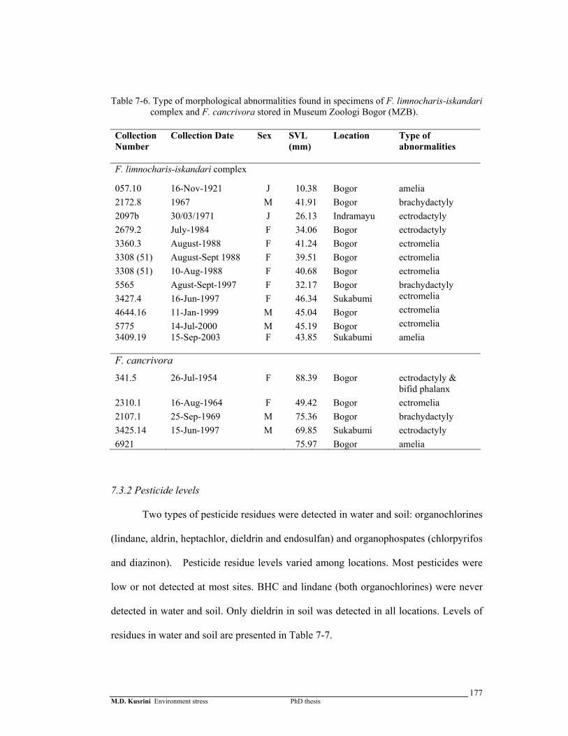
M.D. Kusrini Environment stress PhD thesis
177
Table 7-6. Type of morphological abnormalities found in specimens of F. limnocharis-iskandari
complex and F. cancrivora stored in Museum Zoologi Bogor (MZB). Collection Number
Collection Date Sex SVL (mm)
Location Type of abnormalities
F. limnocharis-iskandari complex
057.10 16-Nov-1921 J 10.38 Bogor amelia 2172.8 1967 M 41.91 Bogor brachydactyly 2097b 30/03/1971 J 26.13 Indramayu ectrodactyly 2679.2 July-1984 F 34.06 Bogor ectrodactyly 3360.3 August-1988 F 41.24 Bogor ectromelia 3308 (51) August-Sept 1988 F 39.51 Bogor ectromelia 3308 (51) 10-Aug-1988 F 40.68 Bogor ectromelia 5565 Agust-Sept-1997 F 32.17 Bogor brachydactyly 3427.4 16-Jun-1997 F 46.34 Sukabumi ectromelia
4644.16 11-Jan-1999 M 45.04 Bogor ectromelia
5775 14-Jul-2000 M 45.19 Bogor ectromelia 3409.19
15-Sep-2003 F 43.85 Sukabumi amelia
F. cancrivora
341.5 26-Jul-1954 F 88.39 Bogor ectrodactyly & bifid phalanx
2310.1 16-Aug-1964 F 49.42 Bogor ectromelia 2107.1 25-Sep-1969 M 75.36 Bogor brachydactyly 3425.14 15-Jun-1997 M 69.85 Sukabumi ectrodactyly 6921 75.97 Bogor amelia
7.3.2 Pesticide levels
Two types of pesticide residues were detected in water and soil: organochlorines
(lindane, aldrin, heptachlor, dieldrin and endosulfan) and organophospates (chlorpyrifos
and diazinon). Pesticide residue levels varied among locations. Most pesticides were
low or not detected at most sites. BHC and lindane (both organochlorines) were never
detected in water and soil. Only dieldrin in soil was detected in all locations. Levels of
residues in water and soil are presented in Table 7-7.
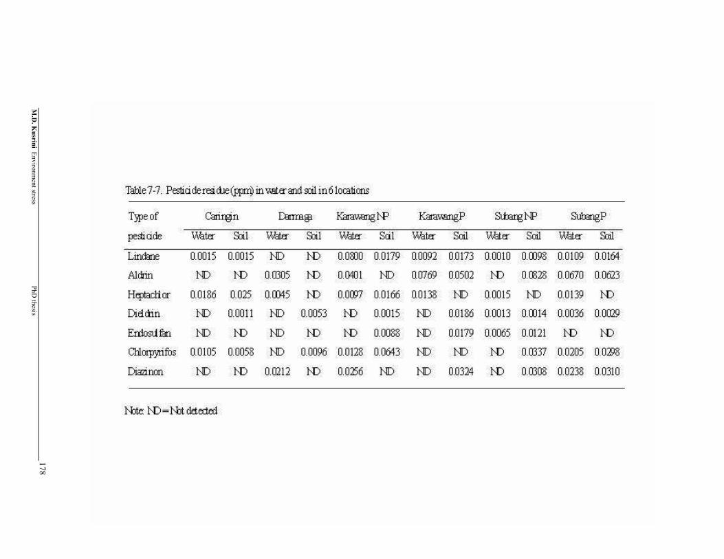
M.D
. Kusrini Environm
ent stress PhD
thesis
178

M.D. Kusrini Environment stress PhD thesis
179
Six organochlorines (BHC, lindane, aldrin, heptachlor, dieldrin and endosulfan)
and three organophosphates (propenofos, chlorpyrifos and diazinon) were detected in
the livers and leg muscles of both species. Pesticide residues in livers were higher than
in leg muscles for both species. Mean levels of organochlorine residues in F.
limnocharis-iskandari complex and F. cancrivora livers and leg muscles were mostly
lower than the maximum residue limit set by the WHO or IHM, except for endosulfan
residues in the liver of F. limnocharis-iskandari complex in Subang NP. However,
some individual frogs exceeded maximum pesticide limits set either by the WHO or
IHM for aldrin, heptachlor, dieldrin and endosulfan.
Organophospate residue limits were exceeded in some locations. Mean
chlorpyrifos residue exceeded limits in F. limnocharis-iskandari complex livers from
Subang NP, also in the livers of F. cancrivora from Karawang NP and Karawang P, and
in the leg muscles of F. cancrivora from Subang P. One F. limnocharis-iskandari
complex from Subang P also exceeded the chlorpyrifos residue limit.
At Karawang NP and Karawang P the livers of both F. limnocharis-iskandari
complex and F. cancrivora had mean values of propenofos residues higher than the
maximum residue limits set by the WHO and IHM. Mean values of propenofos residue
for F. cancrivora leg muscles in the Subang P and mean residue for F. limnocharis-
iskandari complex livers in Darmaga were also higher than the maximum residue level.
Diazinon levels in livers of F. limnocharis-iskandari complex from the
Caringin, Karawang NP, Karawang P, Subang P sites, and also in leg muscles from
Darmaga, were higher than the maximum residue limit set by the WHO. In F.
cancrivora, mean values for diazinon exceeded the WHO standard only in liver from
the Subang NP site. Summary statistics for levels of pesticide residues in both species
of frogs are provided in Tables 7-8 to 7-11.
M.D. Kusrini Environment stress PhD thesis
180
The MRPP tests indicated that levels of pesticide residues in livers and leg
muscles or did not differ between the species when they were compared across all
locations (P = 0.5012 for differences in mean pesticide residues; P = 0.1534 for
differences of pesticide residues in liver and P = 4280 for differences of pesticide
residues in muscle). However, pesticide residues in the livers of F. limnocharis-
iskandari complex differed significantly among locations (P = 0.011), while there are
no significant differences in pesticide residues in F. cancrivora among all locations.
Tests examining the differences between pairs of locations with and without
current pesticide application showed that there were no significant differences in
pesticide residues in either livers and leg muscles of F. limnocharis-iskandari complex
and F. cancrivora between the Karawang NP and the Karawang P locations or between
the Subang NP and the Subang P locations. There was also no significant difference in
pesticide residues in both livers and leg muscles for F. limnocharis-iskandari complex
between the Darmaga and Caringin sites.
Comparisons between regions showed that there were significant differences in
pesticide residues in the livers of F. cancrivora (P = 0.0339), and in mean pesticide
residues in both tissues of F. limnocharis-iskandari complex, between Karawang and
Subang (P = 0.0317). However, there were no significant differences of pesticide
residues in either species between Karawang and Bogor or Subang and Bogor.
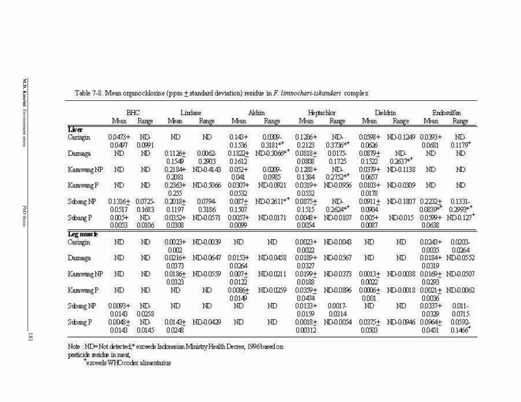
M.D
. Kusrini Environm
ent stress PhD
thesis
181

M.D
. Kusrini Environm
ent stress PhD
thesis
182
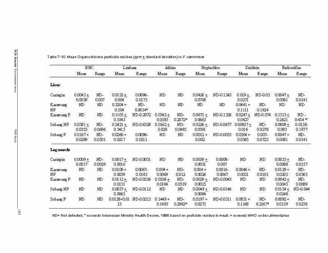
M.D
. Kusrini Environm
ent stress PhD
thesis
183
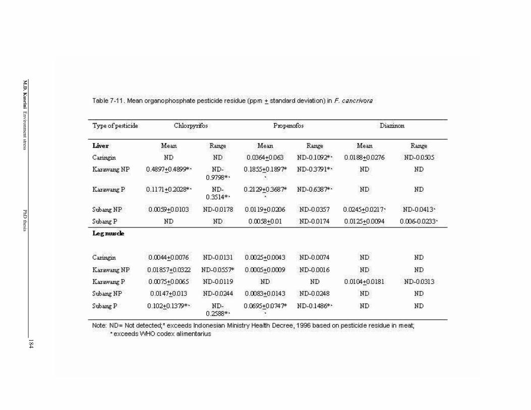
M.D
. Kusrini Environm
ent stress PhD
thesis
184

M.D. Kusrini Environment stress PhD thesis
185
Tables 7-12 and 7-13 summarise the results of comparisons of levels of pesticide
residues for both species among locations, and Figures 7-5 to 7-10 show the mean
pesticide residues in water, soil and frogs in six locations.
Table 7-12. Differences of pesticide residues between pair of location
Questions
Karawang NP vs. Karawang P
Subang NP vs. Subang P
Caringin vs. Darmaga
Is there a significant difference of pesticide residue content in liver and leg muscle in F. limnocharis-iskandari complex?
NO NO YES
Is there a significant difference of pesticide residue content in liver and leg muscle in F. cancrivora?
NO NO N/A
N/A = not available, there is no sample for pesticide content in F. cancrivora in Darmaga
Table 7-13. Differences of pesticide residues between pair of region
Questions
Karawang vs. Subang
Karawang vs. Bogor
Subang vs. Bogor
Is there a significant difference of pesticide residue content in liver in F. limnocharis-iskandari complex?
NO NO NO
Is there a significant difference of pesticide residue content in leg muscle in F. limnocharis-iskandari complex?
NO NO NO
Is there a significant difference of mean pesticide residue content in F. limnocharis-iskandari complex?
YES NO NO
Is there a significant difference of pesticide residue content in liver in F. cancrivora?
YES NO NO
Is there a significant difference of pesticide residue content in leg muscle in F. cancrivora?
NO NO NO
Is there a significant difference of mean pesticide residue content in F. cancrivora?
NO NO NO

M.D. Kusrini Environment stress PhD thesis
186
Caringin
0.00
0.02
0.04
0.06
0.08
0.10
0.12
0.14
0.16
BHC
Linda
neAldr
in
Heptac
hlor
Dieldri
n
Endos
ulfan
Chlorpy
rifos
Propen
ofos
Diazino
n
resi
dues
con
cent
ratio
n (p
pm)
Water Soil
limno liver cancri liverlimno muscle cancri muscle
Figure 7-5. Mean pesticide residues (ppm) in water, soil, livers and leg muscles of F.
limnocharis-iskandari complex and F. cancrivora in Caringin
Darmaga
0.00
0.02
0.04
0.06
0.08
0.10
0.12
0.14
0.16
0.18
0.20
BHC
Linda
neAldr
in
Heptac
hlor
Dieldri
n
Endos
ulfan
Chlorpy
rifos
Propen
ofos
Diazino
n
resi
dues
con
cent
ratio
n
Water Soillimno liver limno muscle
Figure 7-6. Mean pesticide residues (ppm) in water, soil, livers and leg muscles of F.
limnocharis-iskandari complex and F. cancrivora in Darmaga
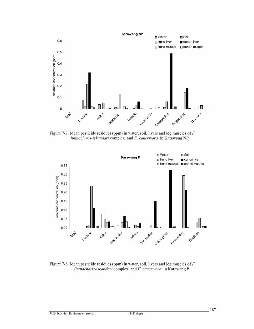
M.D. Kusrini Environment stress PhD thesis
187
Karawang NP
0
0.1
0.2
0.3
0.4
0.5
0.6
BHC
Linda
neAldr
in
Heptac
hlor
Dieldri
n
Endos
ulfan
Chlorpy
rifos
Propen
ofos
Diazino
n
resi
dues
con
cent
ratio
n (p
pm)
Water Soillimno liver cancri liverlimno muscle cancri muscle
Figure 7-7. Mean pesticide residues (ppm) in water, soil, livers and leg muscles of F.
limnocharis-iskandari complex and F. cancrivora in Karawang NP
Karawang P
0.00
0.05
0.10
0.15
0.20
0.25
0.30
0.35
BHC
Linda
neAldr
in
Heptac
hlor
Dieldri
n
Endos
ulfan
Chlorpy
rifos
Propen
ofos
Diazino
n
resi
dues
con
cent
ratio
n (p
pm)
Water Soillimno liver cancri liverlimno muscle cancri muscle
Figure 7-8. Mean pesticide residues (ppm) in water, soil, livers and leg muscles of F.
limnocharis-iskandari complex and F. cancrivora in Karawang P
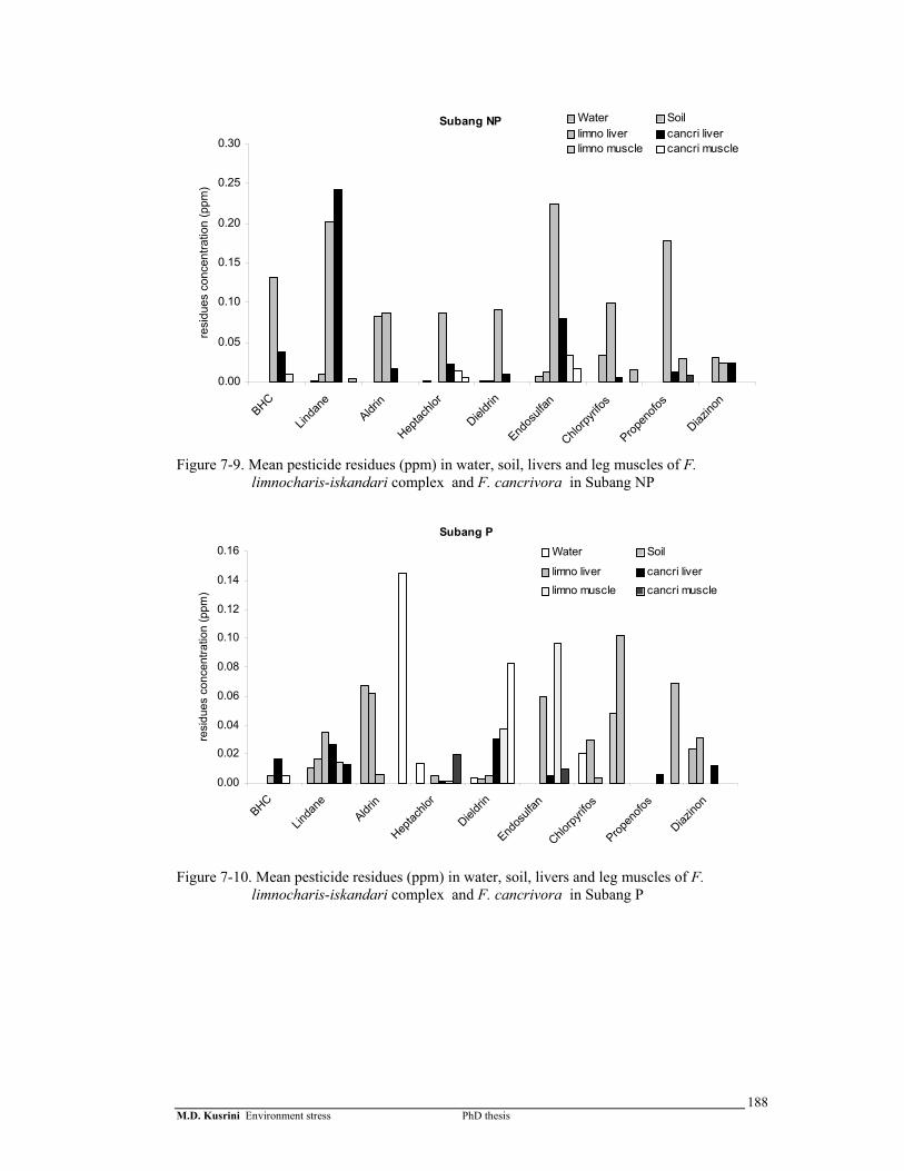
M.D. Kusrini Environment stress PhD thesis
188
Subang NP
0.00
0.05
0.10
0.15
0.20
0.25
0.30
BHC
Linda
neAldr
in
Heptac
hlor
Dieldri
n
Endos
ulfan
Chlorpy
rifos
Propen
ofos
Diazino
n
resi
dues
con
cent
ratio
n (p
pm)
Water Soillimno liver cancri liverlimno muscle cancri muscle
Figure 7-9. Mean pesticide residues (ppm) in water, soil, livers and leg muscles of F.
limnocharis-iskandari complex and F. cancrivora in Subang NP
Subang P
0.00
0.02
0.04
0.06
0.08
0.10
0.12
0.14
0.16
BHC
Linda
neAldr
in
Heptac
hlor
Dieldri
n
Endos
ulfan
Chlorpy
rifos
Propen
ofos
Diazino
n
resi
dues
con
cent
ratio
n (p
pm)
Water Soil
limno liver cancri liverlimno muscle cancri muscle
Figure 7-10. Mean pesticide residues (ppm) in water, soil, livers and leg muscles of F.
limnocharis-iskandari complex and F. cancrivora in Subang P
M.D. Kusrini Environment stress PhD thesis
189
7.3.3 Fluctuating Asymmetry
Overall results for FA appear in tables 7-14 to 7-17. Analyses of log transformed
data showed that there is no directional asymmetry present in either sex of F.
limnocharis-iskandari complex in 2002 and 2003. FA plus antisymmetry formed a
significant proportion of the measured departures from symmetry in F. limnocharis-
iskandari complex but not in F. cancrivora. I therefore excluded F. cancrivora from
further analyses.
The level of unsigned asymmetry for each character in F. limnocharis-iskandari
complex during 2002 and 2003 did not significantly differ between males and females
(Table 7-18). In F. limnocharis-iskandari complex, forelimbs were significantly more
asymmetrical than hindlimbs at all locations during 2002 and 2003 (Table 7-19).
Figures 7-11 and 7-12 show the mean asymmetries + 95 % confidence intervals in each
characters for F. limnocharis-iskandari complex.
ANOVAs comparing levels of unsigned asymmetry across years with location
disregarded showed that levels of asymmetry were higher in male forelimbs (F1,109 =
17.733; P = 0.000) and hindlimbs (F1,109 = 5.770; P = 0.018) in 2002 than in 2003; while
for females it was higher in forelimbs (F1,154 = 10.970; P = 0.001) in 2002 than in 2003
but hindlimbs did not differ significantly (F1,154 = 0.003; P = 0.954). Table 7-20 details
the outcomes of tests for differences in levels of asymmetry between years in F.
limnocharis-iskandari complex from each location.

M.D
. Kusrini Environm
ent stress PhD
thesis
190
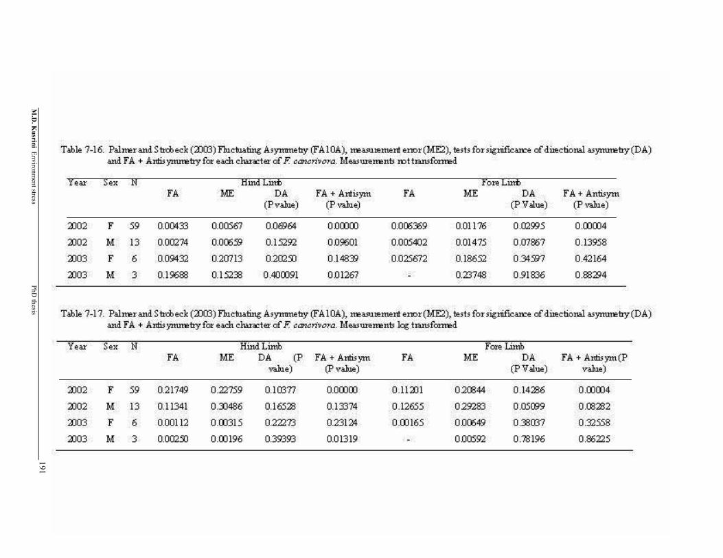
M.D
. Kusrini Environm
ent stress PhD
thesis
191
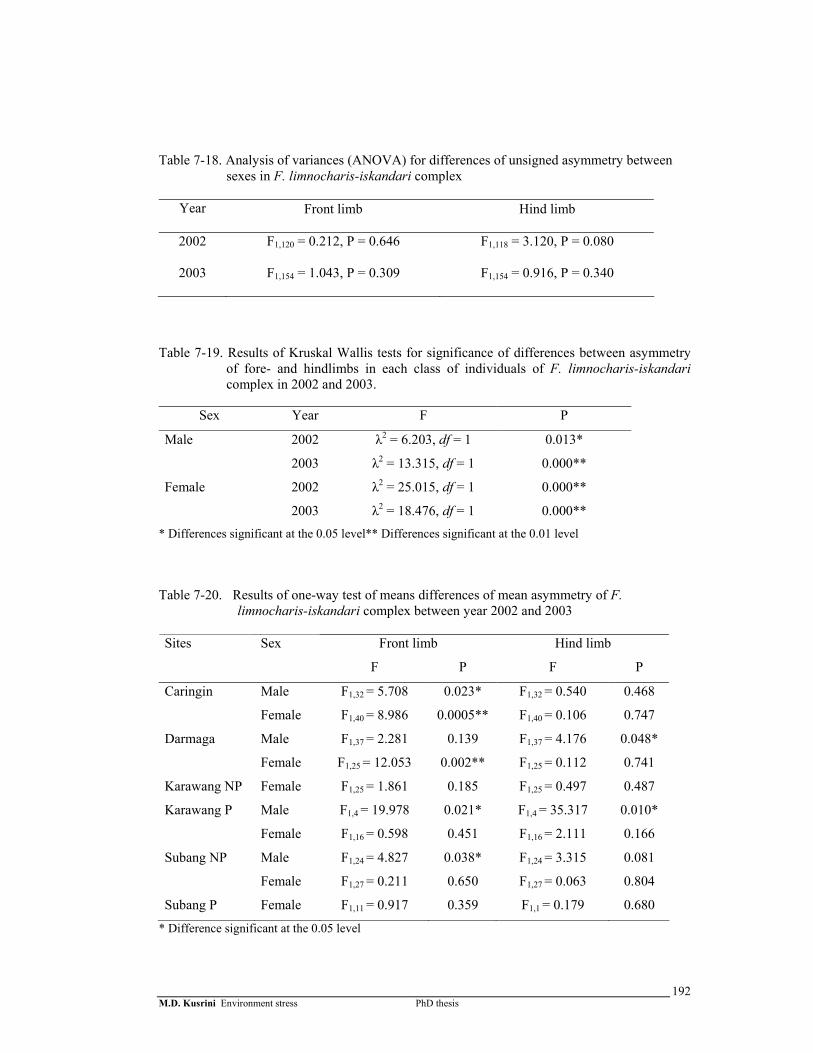
M.D. Kusrini Environment stress PhD thesis
192
Table 7-18. Analysis of variances (ANOVA) for differences of unsigned asymmetry between
sexes in F. limnocharis-iskandari complex
Year Front limb Hind limb
2002 F1,120 = 0.212, P = 0.646 F1,118 = 3.120, P = 0.080
2003 F1,154 = 1.043, P = 0.309 F1,154 = 0.916, P = 0.340
Table 7-19. Results of Kruskal Wallis tests for significance of differences between asymmetry
of fore- and hindlimbs in each class of individuals of F. limnocharis-iskandari complex in 2002 and 2003.
Sex Year F P
Male 2002 λ2 = 6.203, df = 1 0.013*
2003 λ2 = 13.315, df = 1 0.000**
Female 2002 λ2 = 25.015, df = 1 0.000**
2003 λ2 = 18.476, df = 1 0.000** * Differences significant at the 0.05 level** Differences significant at the 0.01 level
Table 7-20. Results of one-way test of means differences of mean asymmetry of F.
limnocharis-iskandari complex between year 2002 and 2003
Front limb Hind limb Sites Sex
F P F P
Caringin Male F1,32 = 5.708 0.023* F1,32 = 0.540 0.468
Female F1,40 = 8.986 0.0005** F1,40 = 0.106 0.747
Darmaga Male F1,37 = 2.281 0.139 F1,37 = 4.176 0.048*
Female F1,25 = 12.053 0.002** F1,25 = 0.112 0.741
Karawang NP Female F1,25 = 1.861 0.185 F1,25 = 0.497 0.487
Karawang P Male F1,4 = 19.978 0.021* F1,4 = 35.317 0.010*
Female F1,16 = 0.598 0.451 F1,16 = 2.111 0.166
Subang NP Male F1,24 = 4.827 0.038* F1,24 = 3.315 0.081
Female F1,27 = 0.211 0.650 F1,27 = 0.063 0.804
Subang P Female F1,11 = 0.917 0.359 F1,1 = 0.179 0.680
* Difference significant at the 0.05 level
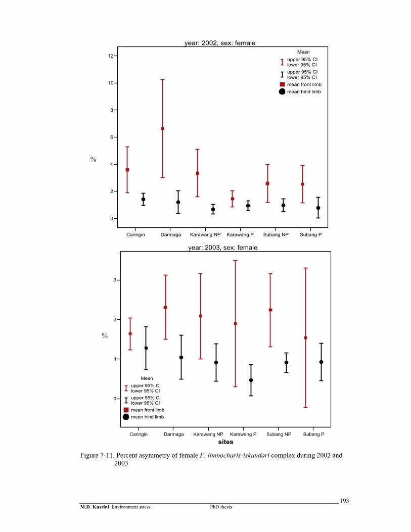
M.D. Kusrini Environment stress PhD thesis
193
Caringin Darmaga Karawang NP Karawang P Subang NP Subang P
sites
0
2
4
6
8
10
12Mean
upper 95% CIlower 95% CIupper 95% CIlower 95% CImean front limbmean hind limb
year: 2002, sex: female
Caringin Darmaga Karawang NP Karawang P Subang NP Subang P
sites
0
1
2
3
Meanupper 95% CIlower 95% CIupper 95% CIlower 95% CImean front limbmean hind limb
year: 2003, sex: female
Figure 7-11. Percent asymmetry of female F. limnocharis-iskandari complex during 2002 and
2003
%
%

M.D. Kusrini Environment stress PhD thesis
194
Caringin Darmaga Subang NP Subang P
sites
-5
0
5
10
15 Meanupper 95% CIlower 95% CIupper 95% CIlower 95% CImean front limbmean hind limb
year: 2002, sex: male
Caringin Darmaga Karawang NP Karawang P Subang NP
sites
-2
0
2
4
6Mean
upper 95% CIlower 95% CIupper 95% CIlower 95% CImean front limbmean hind limb
year: 2003, sex: male
Figure 7-12. Percent asymmetry of male F. limnocharis-iskandari complex during 2002 and
2003
%
%

M.D. Kusrini Environment stress PhD thesis
195
For both characters, I tested each sex separately for differences in asymmetry
among sites following a stepwise procedure. Initially, I grouped the locations into three
regions: Bogor (Caringin and Darmaga), Karawang (Karawang NP and Karawang P)
and Subang (Subang NP and Subang P). Pairwise tests for each character in each sex of
each species between regions indicated that there were no significant differences in any
character or sex between the Karawang and Subang regions; I therefore combined the
data for Karawang and Subang into one region (Karawang/Subang) and tested it against
Bogor. With this grouping, there were significant differences of mean asymmetry in
both sexes of F. limnocharis-iskandari complex between the two regions. Table 7-21
summarises these differences.
Table 7-21. Results of tests for differences in mean asymmetry of F. limnocharis-iskandari complex between the Bogor region and the combined Karawang/Subang region
Sex Year Front limb Hind limb
Male 2002 F1,44 = 2.470, P = 0.123 F1,44 = 0.509, P = 0.479
2003 F1,62 = 1.082, P = 0.164 F1,62 = 1.078, P = 0.303
Female 2002 F1,43 = 6.199, P = 0.017* F1,43 = 8.684, P = 0.005**
2003 F1,84 = 5.579, P = 0.020* F1,84 = 0.961, P = 0.330
*Difference significant at the 0.05 level; ** Difference significant at the 0.01 level
Using data from the population study of F limnocharis-iskandari complex from
sampling-1 (2002) and sampling-3 (2003), I found significant correlations between
body condition and snout vent length (rs= -.169, n = 1103, P < 0.0001). Analysis of
variance showed that body condition differed among males, females, and juveniles
(F2,1100 = 8.483, P < 0.0001). The condition indices of males and females were similar,
while juveniles tended to have higher body condition index values.

M.D. Kusrini Environment stress PhD thesis
196
A more detailed analysis showed that significant differences in body condition
among the classes of individuals of F. limnocharis-iskandari complex occurred in
Caringin sampling-1, Darmaga sampling-3, Karawang P sampling-1 and 3, and in
sampling-1 at Subang P (Table 7-22).
As with asymmetry, body condition differed among sites (Table 7-23) and
between sampling times. Overall, there were significant difference in body condition
among all classes of individuals (females, males and juveniles) between 2002 and 2003
(t275 = 3.251, P = 0.001 for females; t308 = 7.029, P < 0.001 for males and t514= 2.614, P
= 0.009 for juveniles). The body condition of all classes was lower in 2003.
Table 7-22. Results of Kruskal-Wallis tests for differences in body condition among males,
females, and juveniles of F. limncoharis in six locations at one or two sampling times.
Location Sampling Chi-square Df Significant
Caringin 1 9.604 2 0.008**
3 1.397 2 0.497
Darmaga 1 4.600 2 0.100
3 7.008 2 0.030*
Karawang NP 1 2.622 2 0.270
3 3.226 2 0.199
Karawang P 1 6.668 2 0.036*
3 110.132 2 0.006**
Subang NP 1 1.273 2 0.529
3 2.796 1 0.095
Subang P 1 6.823 2 0.033*
* Difference significant at the 0.05 level ** Difference significant at the 0.01 level

M.D. Kusrini Environment stress PhD thesis
197
Table 7-23. Results of Kruskal-Wallis tests for differences of in body condition index of F.
limnocharis-iskandari complex among sites.
Sex Sampling Chi-Square Df P
Female 1 6.452 5 0.265
3 23.155 5 <0.001
Male 1 13.496 5 0.019
3 63.207 4 <0.000
Spearman correlations examining possible relationships between individual
body condition and developmental instability levels, as indexed by unsigned fore- and
hindlimb asymmetry, demonstrated no significant relationship for either the forelimbs
(rs = –0.013, n = 262, P = 0.840) or the hindlimbs of F. limnocharis-iskandari complex
(rs = 0.026, n = 262, P = 0.674).
7.3.4 Chythridiomycosis
I examined prepared sections of the toes of 184 individuals (103 F.
limnocharis-iskandari complex, 35 F. cancrivora and 46 L. macrodon. and found no
sign of chytrid infection in any of the samples. All samples had thin layers of outer
epidermal keratin, which is typical of uninfected frogs.
7.4 Discussion
Results on the frequencies of morphological abnormalities indicated that the
frequencies of abnormalities in F. limnocharis-iskandari complex and F. cancrivora in
West Java were relatively low and probably within the normal range (Tyler, 1999 and
Oullet, 2000), although in some cases there were elevated percentages of abnormalities
(>5%). The other two species (Occidozyga lima and Limnonectes kuhlii) in which
abnormalities were detected had sample sizes too small for meaningful estimates of the
frequency of abnormalities. Because my data were collected almost exclusively from
M.D. Kusrini Environment stress PhD thesis
198
late juvenile and adult frogs, I might have found higher frequencies in F. limnocharis-
iskandari complex and F. cancrivora if I had sampled tadpoles or immediately post-
metamorphic frogs, reducing or eliminating the probable effects of differential survival.
Residues of many pesticides were present, some at relatively elevated levels.
The existing pesticide residues in soil, water and frogs reflect the high level of
pesticides used in the recent past, and in some cases at present, by farmers in the habitat.
Research by Ginoga in the Sukamandi rice fields in Subang (1999) revealed that all her
farmer respondents (n=60) used insecticides, sometimes more than one kind. They
were using primarily organophosphates, carbamates and pyrethroids (Ginoga, 1999).
Although most organochlorine pesticides are now usually not used around the world
because of their persistence and impact on health and the environment (Carson, 1962;
Abdullah, 1991) and have been replaced by organophosphates, a small number of
farmers in the Subang area (5%) still used organochlorines as of 1998 (Ginoga, 1999).
The occurrence of organochlorine residues in my study area could result from current
use of this type of pesticide. However, organochlorines have long periods of persistence
in the environment (Carson, 1962; Quisey et al., 1995, VanWyk et al., 2001; Smith and
Gangolli, 2002). Concentrations of organochlorines detected therefore reflect
cumulative patterns of use over an extended time period. Different levels of
organochlorine residues might have been found if adipose tissues, in which these
lipophilic substances accumulate, had been sampled in addition to muscle and liver
(Ayas et al., 1997).
Some individual frogs contained high levels of organochlorine and
organophosphate residues. Ginoga’s research in Subang (1999) revealed that
organochlorine residues were also high in water birds. For instance, Aldrin residues in
the livers of F. limnocharis-iskandari complex frogs in two areas (Darmaga 0.1822
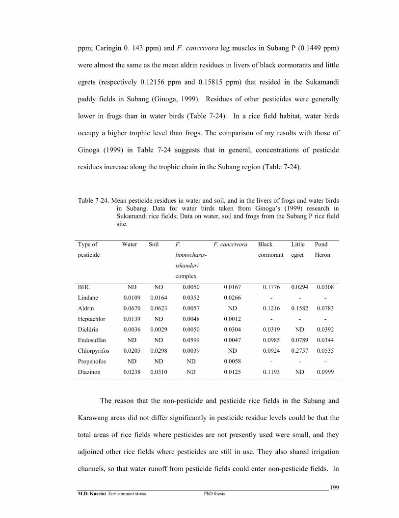
M.D. Kusrini Environment stress PhD thesis
199
ppm; Caringin 0. 143 ppm) and F. cancrivora leg muscles in Subang P (0.1449 ppm)
were almost the same as the mean aldrin residues in livers of black cormorants and little
egrets (respectively 0.12156 ppm and 0.15815 ppm) that resided in the Sukamandi
paddy fields in Subang (Ginoga, 1999). Residues of other pesticides were generally
lower in frogs than in water birds (Table 7-24). In a rice field habitat, water birds
occupy a higher trophic level than frogs. The comparison of my results with those of
Ginoga (1999) in Table 7-24 suggests that in general, concentrations of pesticide
residues increase along the trophic chain in the Subang region (Table 7-24).
Table 7-24. Mean pesticide residues in water and soil, and in the livers of frogs and water birds in Subang. Data for water birds taken from Ginoga’s (1999) research in Sukamandi rice fields; Data on water, soil and frogs from the Subang P rice field site.
Type of
pesticide
Water Soil F.
limnocharis-
iskandari
complex
F. cancrivora Black
cormorant
Little
egret
Pond
Heron
BHC ND ND 0.0050 0.0167 0.1776 0.0294 0.0308
Lindane 0.0109 0.0164 0.0352 0.0266 - - -
Aldrin 0.0670 0.0623 0.0057 ND 0.1216 0.1582 0.0783
Heptachlor 0.0139 ND 0.0048 0.0012 - - -
Dieldrin 0.0036 0.0029 0.0050 0.0304 0.0319 ND 0.0392
Endosulfan ND ND 0.0599 0.0047 0.0985 0.0789 0.0344
Chlorpyrifos 0.0205 0.0298 0.0039 ND 0.0924 0.2757 0.0535
Propenofos ND ND ND 0.0058 - - -
Diazinon 0.0238 0.0310 ND 0.0125 0.1193 ND 0.0999
The reason that the non-pesticide and pesticide rice fields in the Subang and
Karawang areas did not differ significantly in pesticide residue levels could be that the
total areas of rice fields where pesticides are not presently used were small, and they
adjoined other rice fields where pesticides are still in use. They also shared irrigation
channels, so that water runoff from pesticide fields could enter non-pesticide fields. In

M.D. Kusrini Environment stress PhD thesis
200
fact, it could be suggested that in terms of pest reduction, non-pesticide rice fields were
actually benefiting from the pesticide rice fields because they were getting similar
concentrations pesticides without the need to buy them. The lack of differences in
concentrations in frog tissues could reflect movements of frogs between fields, as
demonstrated in chapter 5. Frogs frequently move between blocks of rice fields, leaving
dry blocks for those with higher water levels, and are thus likely to move between fields
where pesticides are not applied and those where they are.
In terms of food products, the detection of some residues in the leg muscles of
both species of rice field’s frog indicates that frog legs originating from rice fields could
pose a health risk for human consumption. I suggest further pesticide monitoring in this
area to obtain further data on levels of pesticide residues in frogs and the environment.
These may suggest that pesticide use should be moderated to minimize potential
adverse impacts on human health and the environment.
My results showed that levels of asymmetry differed between characters. The
same result was also mentioned by McCoy and Harris (2003) in salamanders. For
fluctuating asymmetry in the fields, I suggest measuring multiple characters to gather
more information.
Unsigned asymmetry did not differ between the Karawang or Subang pesticide
and non-pesticide sites for either the forelimbs or the hindlimbs of either sex of F.
limnocharis-iskandari complex. These results are in accordance with the finding that
there are no differences in pesticide residue levels between the non-pesticide and
pesticide sites. Frogs in Indonesian rice fields have been exposed to pesticides for many
years (Figure 7-13) and may have developed resistance to any direct negative effects
they may have experienced from pesticides. Since there are no data on asymmetry

M.D. Kusrini Environment stress PhD thesis
201
levels in rice field frogs before pesticide use, it is uncertain if the levels of asymmetry I
found were elevated at all sites in response to pesticide use.
Insecticide (kg/ha)
Figure 7-13. Pesticide and insecticide use (kg/ha)in rice fields in Indonesia. Data from
Statistical Bureau (BPS).
Juveniles of F. limnocharis-iskandari complex tended to have better body
condition than adults. This could reflect greater selection for good body condition acting
on survival in juveniles, or could reflect changes in allocation of resources, with adults
investing more energy in reproduction.
There were no significant correlations correlation between asymmetry and body
condition in F. limnocharis-iskandari complex. Interpretation of this relationship is
complicated by comparisons among years. Results showed that both asymmetry and the
body condition of F. limnocharis-iskandari complex were lower in 2003. If higher
asymmetry reflects greater stress, which produces lower body condition, then the results
would show a lower body condition in all classes of individuals during 2002, not in
2003.
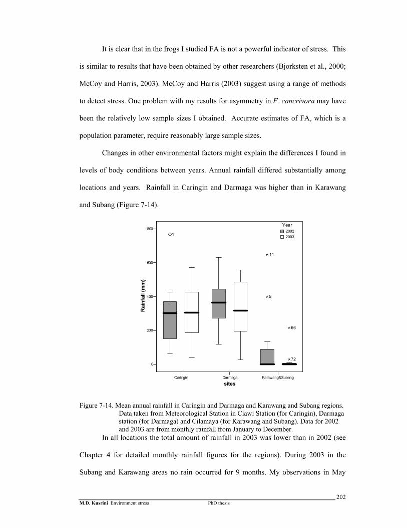
M.D. Kusrini Environment stress PhD thesis
202
It is clear that in the frogs I studied FA is not a powerful indicator of stress. This
is similar to results that have been obtained by other researchers (Bjorksten et al., 2000;
McCoy and Harris, 2003). McCoy and Harris (2003) suggest using a range of methods
to detect stress. One problem with my results for asymmetry in F. cancrivora may have
been the relatively low sample sizes I obtained. Accurate estimates of FA, which is a
population parameter, require reasonably large sample sizes.
Changes in other environmental factors might explain the differences I found in
levels of body conditions between years. Annual rainfall differed substantially among
locations and years. Rainfall in Caringin and Darmaga was higher than in Karawang
and Subang (Figure 7-14).
Caringin Darmaga Karawang&Subang
sites
0
200
400
600
800
Rai
nfal
l (m
m)
1
5
11
72
66
Year20022003
Figure 7-14. Mean annual rainfall in Caringin and Darmaga and Karawang and Subang regions. Data taken from Meteorological Station in Ciawi Station (for Caringin), Darmaga station (for Darmaga) and Cilamaya (for Karawang and Subang). Data for 2002 and 2003 are from monthly rainfall from January to December.
In all locations the total amount of rainfall in 2003 was lower than in 2002 (see
Chapter 4 for detailed monthly rainfall figures for the regions). During 2003 in the
Subang and Karawang areas no rain occurred for 9 months. My observations in May
M.D. Kusrini Environment stress PhD thesis
203
2003 showed that most rice field areas failed to produce because irrigation could not
supply water because of water shortages in major reservoirs. Lowered body conditions
in 2003 could thus have been produced by the short-term effects of water stress, or by
food shortages or behavioural changes associated with the relatively low availability of
water.
Chytridiomycosis has been found infecting amphibians almost worldwide
(Berger et al., 1999). Chytridomycosis had not been looked for in samples from
Indonesian frogs before my study, and my results show that at least for three species of
frogs occurring in West Java, there is no evidence of infection by the amphibian chytrid.
In Australia, chytrid prevalences are higher and frogs are more likely to be negatively
affected by the amphibian chytrid at higher elevation, cooler sites with permanent water
(Berger et al. 1998, 2004). Most paddy fields in Indonesia occur in lowland areas and
the habitats experience periodic wet and dry phases. A dry phase during the fallow
period can last for more than one month, potentially eliminating the amphibian chytrid
from the environment. Frogs like L. macrodon that live at higher elevations in
association with more permanent water may be at greater risk, and much additional
sampling is needed before Indonesia can be declared to be free of the amphibian chytrid
fungus.
My results suggest that environmental stress affected F. limnocharis-iskandari
complex more than F. cancrivora. This is indicated by the occurrence of morphological
abnormalities in F. limnocharis-iskandari complex on almost all sampling occasions at
all locations. One possible source of stress that could have affected F. limnocharis-
iskandari complex more than F. cancrivora is population density. In almost all
sampling locations, the densities of F. limnocharis-iskandari complex were
substantially higher than those of F. cancrivora (Chapter 5). However, since both
M.D. Kusrini Environment stress PhD thesis
204
species are abundant in rice fields, it seems that both F. limnocharis-iskandari complex
and F. cancrivora can cope effectively with any environmental stresses peculiar to these
habitats.
M.D. Kusrini Conservation Status PhD thesis
205
CHAPTER 8
CONSERVATION STATUS OF THE EDIBLE FROGS
8.1 Introduction
It is known (Chapters 2 and 3) that large numbers of frogs are harvested
annually in Indonesia for export and the domestic market. Conservationists have
queried whether this threatens the survival of the harvested species (Barfield, 1986;
Niekisch, 1986; Martens, 1991, Patel, 1993; Primack, 1999; Schmuck, 2000).
Answering this question can be approached by 1) applying a model of the population
dynamics of the harvested frogs that includes harvesting rate, and 2) evaluating data on
the population biology and distribution of the harvested species in light of criteria for
assessing conservation status, i.e. the IUCN Red Categories and the CITES Res. Conf.
9.24 on the Criteria for Amendment of Appendices I and II.
Assessment of sustainable harvesting is a complex task, and requires examining
ecological, biological and economic issues. Examining these complex issues requires
simplifying real-life systems into models that can be simulated using computer tools
(Chi, 2000). Assessments of harvesting for several species, mostly mammals, have used
this modelling approach (Slade et al., 1998; Hurtado-Gonzales and Bodmer, 2004).
These models attempt to simulate the dynamics of a system, identifying components
and processes by which they interact (Odum, 1971; Jeffers, 1978). The system is
decomposed into state variables (stocks) and rates of change between stocks
(parameters or flows), and a model is assembled connecting them. These models are
often characterized by internal feedback mechanisms, such as nonlinearities, delays and
uncertainties (Sterman, 1992). These basics (feedback, stocks and flows, time delays,
nonlinearities) are essential foundations for effective systems thinking and modeling.
M.D. Kusrini Conservation Status PhD thesis
206
Once a model is assembled and its parameters are well enough known, it can be used to
predict whether harvesting is sustainable, and to examine the sensitivity of sustainability
to changes or inaccurate estimates of parameters.
In the early development of modeling, simulations usually used complex custom
computer programs in relatively low-level languages such as FORTRAN, BASIC, and
C. More recently, modeling and simulation development has been simplified by the
development of symbolic modeling tools such as Powersim and STELLA (Chi, 2000).
Assessing the conservation status of species is another approach that can be used
to evaluate the impact of harvesting. For example, Soehartono and Mardiastuti (2002)
performed a series of assessments on Indonesian wildlife species (i.e. arowana fish,
monkey, swiflets and ramin plants) to determine whether they appeared to be threatened
by trade.
From my previous chapters, it is clear only two of the three species I studied (F.
cancrivora and L. macrodon) are important in the Indonesian frog leg trade. The small
size of F. limnocharis-iskandari complex makes it unsuitable for export, and even in the
domestic market, only relatively small numbers of this species are sold (Chapter 2 and
3). The populations of F. limnocharis-iskandari complex in the study areas were high
(Chapter 5) and it is known that this species is distributed widely in Indonesia (Chapter
4). As such, this chapter will focus on the conservation status of F. cancrivora and L.
macrodon.
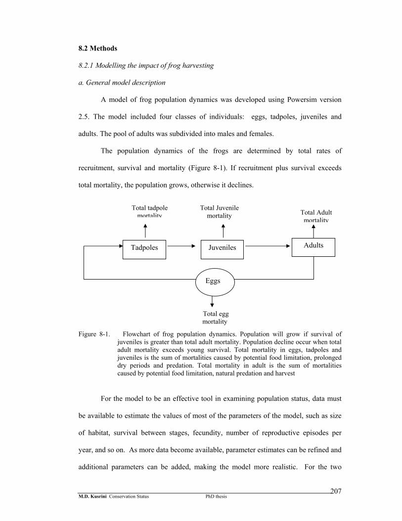
M.D. Kusrini Conservation Status PhD thesis
207
8.2 Methods
8.2.1 Modelling the impact of frog harvesting
a. General model description
A model of frog population dynamics was developed using Powersim version
2.5. The model included four classes of individuals: eggs, tadpoles, juveniles and
adults. The pool of adults was subdivided into males and females.
The population dynamics of the frogs are determined by total rates of
recruitment, survival and mortality (Figure 8-1). If recruitment plus survival exceeds
total mortality, the population grows, otherwise it declines.
Figure 8-1. Flowchart of frog population dynamics. Population will grow if survival of
juveniles is greater than total adult mortality. Population decline occur when total adult mortality exceeds young survival. Total mortality in eggs, tadpoles and juveniles is the sum of mortalities caused by potential food limitation, prolonged dry periods and predation. Total mortality in adult is the sum of mortalities caused by potential food limitation, natural predation and harvest
For the model to be an effective tool in examining population status, data must
be available to estimate the values of most of the parameters of the model, such as size
of habitat, survival between stages, fecundity, number of reproductive episodes per
year, and so on. As more data become available, parameter estimates can be refined and
additional parameters can be added, making the model more realistic. For the two
Tadpoles Juveniles Adults
Total egg mortality
Total tadpole mortality
Total Juvenilemortality Total Adult
mortality
Eggs

M.D. Kusrini Conservation Status PhD thesis
208
species I studied, there were sufficient data in my study and in the literature to estimate
enough parameters to model the dynamics of F. cancrivora. I therefore used my model
to simulate the dynamics of F. cancrivora on the island of Java.
b. Harvesting simulation model
A flowchart of my model of frog population dynamics, including most relevant
aspects of frog ecology and harvesting, is presented in Figure 8-2. I simplified this
model by focusing only on frog population sizes and harvesting, omitting the explicit
consideration of natural predator population sizes and food availability. The impacts of
predator population size and food availability are still included, since they affect rates of
survival.
Figure 8-2. Diagram of systems that influence the population of frog. Frog population depends
on food availability, habitat, natural predator population and harvest
The frog’s preferred habitat will vary among species. F. cancrivora is most
abundant in wet rice fields or sawah, so the area of these is used as the area of habitat
Frog population
Harvest
Habitat
Food availability Natural predator population
(-)
(+) (+)
(-)
(-)
(+)
(+)

M.D. Kusrini Conservation Status PhD thesis
209
available. This area, in hectares, is taken from estimates for Java in 1999, published by
the Indonesian Statistical Bureau.
Data on the biology and ecology of F. cancrivora from my study and published
studies were used to estimate parameters affecting their recruitment and survival.
Church (1970), Berry (1975), and Premo (1985) have published very high estimates of
fecundity for this species based on dissections, which is up to 10,000 eggs. Iskandar
(1998) and Jaafar (1994), who counted eggs in spawned clutches, estimate 1,000 eggs
per clutch. This discrepancy suggests that females may lay several clutches in quick
succession within a breeding season. All authors agree that F. cancrivora breed year
round, but that peaks in reproductive activity usually occur twice a year. The timing of
breeding is related to the timing of water level in the rice fields (Jaafar, 1994 and this
study). Jaafar (1994) concluded that females could produce multiple clutches per
season. Rice planting usually occurs two to three times in a year, thus I assume that
breeding could occur up to four times a year (two major breeding episodes per
reproductive season times two seasons), with between 1,000 and 10,000 eggs deposited
per major breeding episode.
Of the eggs spawned in each year, a proportion die before hatching. Eggs that
survive enter the tadpole stage. A relatively high proportion of tadpoles die before
metamorphosis; those that survive enter the terrestrial juvenile stage. Rates of survival
of eggs and tadpoles were obtained from Jaafar (1994), who estimated rates as 0.06 and
0.05 respectively.
Rates of survival of F. cancrivora through the terrestrial juvenile stage have not
been measured. As an initial estimate, I used the juvenile survival rate of Rana grylio, a
pond frog harvested in the United States, which is 0.72 (Wood et al., 1998). This
estimate is relatively high, and as part of my analysis I examined the implications of
M.D. Kusrini Conservation Status PhD thesis
210
other possible patterns of juvenile survival. Adult frogs will breed and eventually leave
the system either through death or emigration. The model assumes that there is no
immigration and emigration into the system since it simulates the aggregate population
of all rice fields in Java.
The model assumes that there are two causes of adult frog mortality: 1) natural
mortality, which includes such factors as drying, food limitation, and predation and 2)
harvest. I combined natural mortality rates into a single parameter, which I kept separate
from harvesting rate. For each run of the model, all rates are constant; they do not
depend on density.
From the data on total frog leg exports from 1969 – 2003 (Chapter 2), it appears
that the annual total number of frogs exported increased from 1969 to approximately
1993, and has since remained approximately constant, with some fluctuations. The data
I collected on domestic harvesting (Chapter 3) indicated that in 2003-2004 the domestic
harvest was approximately seven times the export harvest; for the model I have assumed
that this ratio remains constant. The total harvest of frogs is estimated based from the
highest number of frogs exported from Java (1993) times 0.75 (the proportion of
harvested frogs that are F. cancivora) times 8, which adds in the sevenfold larger
harvest for domestic purposes. Based on estimated harvest using actual data from
harvesters (Chapter 3), the range of harvest for 1993 is 200 – 600 million, with a modal
estimate of 400 million.
The initial number of mature frogs is based on the mean density of F. cancrivora
(40 individuals/ha) estimated in my mark-recapture study (Chapter 5), multiplied by the
habitat size (3,375,381 ha). The initial number of juveniles is also based on the mean
density of juvenile F. cancrivora estimated from my study.
M.D. Kusrini Conservation Status PhD thesis
211
Jaafar (1994) estimated that F. cancrivora is short-lived (maximum 2-3 years).
The female to male adult ratio in the field varied from 0.3:1 to 1.3:1 (Chapter 5).
Because females were mostly taken (ratio of female: male harvest was 2: 1, see Chapter
3), I put the fraction of females in the population as 0.3 and males as 0.7. It is possible
that many females lived as little as one year after reaching maturity. In order to produce
conservative estimates, I set the model to allow each female to breed only four times,
assuming assumed that year-to-year survival of adult frogs is zero. All females were
assumed able to breed before they were taken. The simulation time is expressed in
years.
To examine the sensitivity of this model to my parameter estimates and
assumptions, I varied several parameters (juvenile survival rate, times breeding in a
year, and harvest rate) while holding the values of other parameters constant. I
evaluated the behaviour of the model by running it for 20 years for each set of
parameters. Because I did not incorporate density dependence into the model, it is not
realistic to expect it to stabilize at a constant population size. I classified the outcome of
each run as either positive, if the population was predicted to be increasing at year 20,
or negative, if the population was predicted to be decreasing. Table 8-1 shows the
equations and numbers used in the simulation.
8.2.2. Conservation status
To assess their conservation status, I examined the properties of both frogs
against criteria for IUCN Red List and the CITES Res. Conf. 9.24 on the Criteria for
Amendment of Appendices I and II.
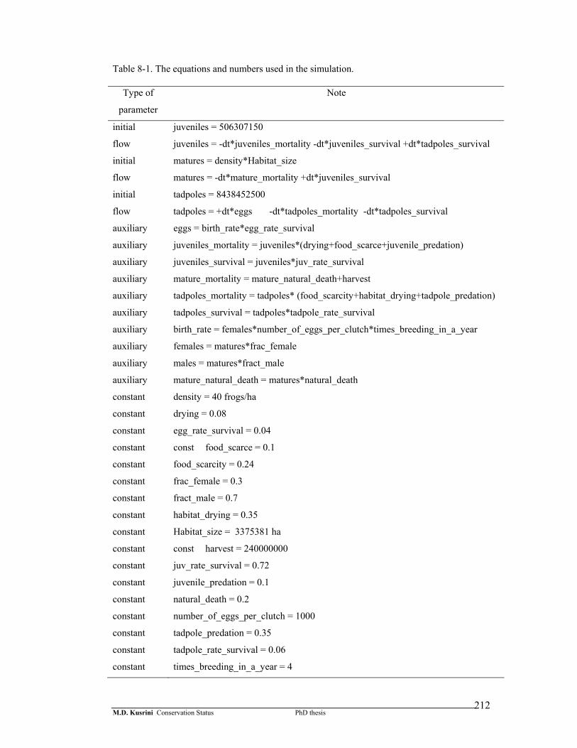
M.D. Kusrini Conservation Status PhD thesis
212
Table 8-1. The equations and numbers used in the simulation.
Type of
parameter
Note
initial juveniles = 506307150
flow juveniles = -dt*juveniles_mortality -dt*juveniles_survival +dt*tadpoles_survival
initial matures = density*Habitat_size
flow matures = -dt*mature_mortality +dt*juveniles_survival
initial tadpoles = 8438452500
flow tadpoles = +dt*eggs -dt*tadpoles_mortality -dt*tadpoles_survival
auxiliary eggs = birth_rate*egg_rate_survival
auxiliary juveniles_mortality = juveniles*(drying+food_scarce+juvenile_predation)
auxiliary juveniles_survival = juveniles*juv_rate_survival
auxiliary mature_mortality = mature_natural_death+harvest
auxiliary tadpoles_mortality = tadpoles* (food_scarcity+habitat_drying+tadpole_predation)
auxiliary tadpoles_survival = tadpoles*tadpole_rate_survival
auxiliary birth_rate = females*number_of_eggs_per_clutch*times_breeding_in_a_year
auxiliary females = matures*frac_female
auxiliary males = matures*fract_male
auxiliary mature_natural_death = matures*natural_death
constant density = 40 frogs/ha
constant drying = 0.08
constant egg_rate_survival = 0.04
constant const food_scarce = 0.1
constant food_scarcity = 0.24
constant frac_female = 0.3
constant fract_male = 0.7
constant habitat_drying = 0.35
constant Habitat_size = 3375381 ha
constant const harvest = 240000000
constant juv_rate_survival = 0.72
constant juvenile_predation = 0.1
constant natural_death = 0.2
constant number_of_eggs_per_clutch = 1000
constant tadpole_predation = 0.35
constant tadpole_rate_survival = 0.06
constant times_breeding_in_a_year = 4
M.D. Kusrini Conservation Status PhD thesis
213
8.3 Results
8.3.1 Population models including harvesting
a. The simulation
Figure 8-3 shows the population dynamic model for F. cancrivora. I used the
simulation to explore the implications of harvesting and variation in vital rates for the
total Javan population of this species as described in the methods. Populations
fluctuated considerably for the first 5-years before either increasing or decreasing
steadily in numbers (Figures 8-4, 8-5). These initial fluctuations occur as the population
approaches its stable age distribution. Tables 8-2 and 8-3 summarise the impact of
variation in harvesting rates, fecundity, number of major reproductive episodes per year,
and changes in juvenile survival to reproduction on the sustainability of the Javan
population of F. cancrivora. The results show under a variety of parameter
combinations and harvesting rates, the estimated total harvest (between 100,000,000
and 500,000,000 frogs per year) in Java is sustainable. They also show that it is not
sustainable for many parameter combinations. This suggests that the true situation is
that frogs are being harvested at rates very near the boundary between sustainability and
unsustainability.
b. Model limitations
The limitations of this model are mostly caused by lack of information. More
research is needed to improve the estimates of population parameters, for instance the
survival of terrestrial juveniles to maturity and the numbers of times that females
reproduce. It would also be very useful to incorporate the effects of density
dependence, which could lead to lower sensitivity to changes in harvesting rate.
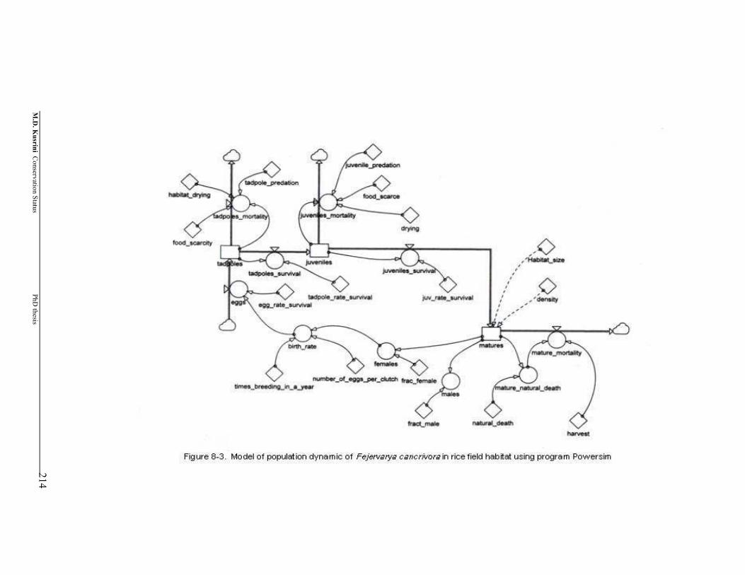
M.D
. Kusrini C
onservation Status PhD
thesis
214
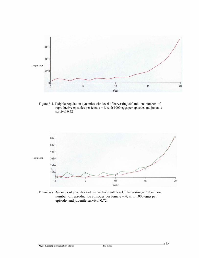
M.D. Kusrini Conservation Status PhD thesis
215
Figure 8-4. Tadpole population dynamics with level of harvesting 200 million, number of reproductive episodes per female = 4, with 1000 eggs per episode, and juvenile survival 0.72
Figure 8-5. Dynamics of juveniles and mature frogs with level of harvesting = 200 million, number of reproductive episodes per female = 4, with 1000 eggs per episode, and juvenile survival 0.72
Population
Population
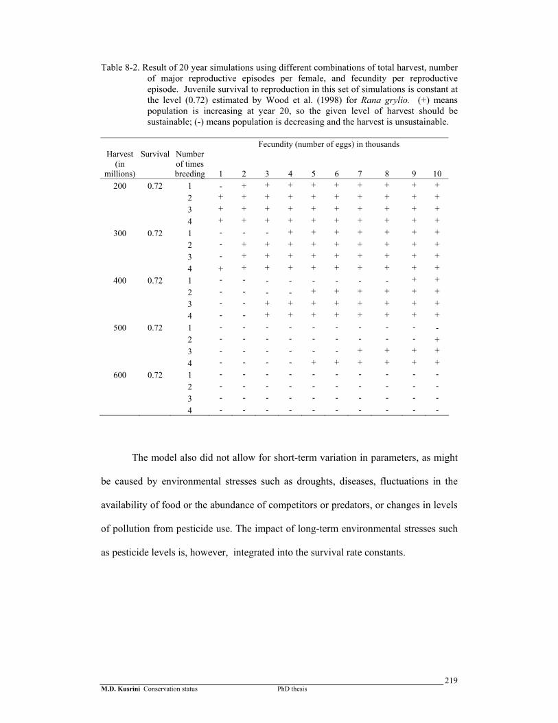
M.D. Kusrini Conservation status PhD thesis
219
Table 8-2. Result of 20 year simulations using different combinations of total harvest, number of major reproductive episodes per female, and fecundity per reproductive episode. Juvenile survival to reproduction in this set of simulations is constant at the level (0.72) estimated by Wood et al. (1998) for Rana grylio. (+) means population is increasing at year 20, so the given level of harvest should be sustainable; (-) means population is decreasing and the harvest is unsustainable.
Fecundity (number of eggs) in thousands
Harvest (in
millions)
Survival
Number of times breeding 1 2 3 4 5 6 7 8 9 10
200 0.72 1 - + + + + + + + + + 2 + + + + + + + + + + 3 + + + + + + + + + + 4 + + + + + + + + + +
300 0.72 1 - - - + + + + + + + 2 - + + + + + + + + + 3 - + + + + + + + + + 4 + + + + + + + + + +
400 0.72 1 - - - - - - - - + + 2 - - - - + + + + + + 3 - - + + + + + + + + 4 - - + + + + + + + +
500 0.72 1 - - - - - - - - - - 2 - - - - - - - - - + 3 - - - - - - + + + + 4 - - - - + + + + + +
600 0.72 1 - - - - - - - - - - 2 - - - - - - - - - - 3 - - - - - - - - - -
4 - - - - - - - - - -
The model also did not allow for short-term variation in parameters, as might
be caused by environmental stresses such as droughts, diseases, fluctuations in the
availability of food or the abundance of competitors or predators, or changes in levels
of pollution from pesticide use. The impact of long-term environmental stresses such
as pesticide levels is, however, integrated into the survival rate constants.
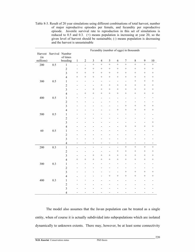
M.D. Kusrini Conservation status PhD thesis
220
Table 8-3. Result of 20 year simulations using different combinations of total harvest, number of major reproductive episodes per female, and fecundity per reproductive episode. Juvenile survival rate to reproduction in this set of simulations is reduced to 0.5 and 0.3. (+) means population is increasing at year 20, so the given level of harvest should be sustainable; (-) means population is decreasing and the harvest is unsustainable
Fecundity (number of eggs) in thousands
Harvest (in
millions)
Survival
Number of times breeding 1 2 3 4 5 6 7 8 9 10
200 0.5 1 - - + + + + + + + + 2 - + + + + + + + + + 3 + + + + + + + + + + 4 + + + + + + + + + +
300 0.5 1 - - - - - - - + + + 2 - - - + + + + + + + 3 - - + + + + + + + + 4 - + + + + + + + + +
400 0.5 1 - - - - - - - - - - 2 - - - - - - - - - - 3 - - - - - - + + + + 4 - - - - - + + + + +
500 0.5 1 - - - - - - - - - - 2 - - - - - - - - - - 3 - - - - - - - - - + 4 - - - - - - + + + +
60 0.5 1 - - - - - - - - - - 2 - - - - - - - - - - 3 - - - - - - - - - - 4 - - - - - - - - - -
200 0.3 1 - - - - - - + + + + 2 - - - - - + + + + + 3 - - + + + + + + + + 4 + + + + + + + + + +
300 0.3 1 - - - - - - - - - - 2 - - - - - - - - - - 3 - - - - - - + + + + 4 - - - - + + + + + +
400 0.3 1 - - - - - - - - - - 2 - - - - - - - - - - 3 - - - - - - - - - - 4 - - - - - - - - - -
The model also assumes that the Javan population can be treated as a single
entity, when of course it is actually subdivided into subpopulations which are isolated
dynamically to unknown extents. There may, however, be at least some connectivity

M.D. Kusrini Conservation status PhD thesis
221
among all of the populations in the island, as it appears from my data (Chapter 5) that
F. cancrivora has low site fidelity (Chapter 5) and moves relatively freely, at least on
a local scale.
8.3.2 Conservation status
Comparisons of the population parameters of F. cancrivora and L. macrodon
to IUCN Red List and the CITES criteria are given in Tables 8-4 to 8-7. From this
assessment F. cancrivora is not qualified for listing in any threat category under
IUCN Red List criteria nor CITES Appendix I and II. On the other hand, more
consideration needs to be given to L. macrodon. This frog seems inappropriate to be
included in CITES Appendix I, however, it is possible that this species might qualify
for listing as vulnerable or in CITES Appendix II if more information was available
on its population biology. Based on my market surveys, in which I found that there
are often hundreds of frogs of this species sold every day, it is clear that the number of
mature L. macrodon currently is more than 10,000 individuals (Chapter 3). The
distribution is also likely to be more than 20,000 km2, since the area of West Java
alone is 34,597 km2 (BPS, 2002). The limited distribution I found for this species
(Chapter 4) could be due to a lack of surveys. I could not make any informed
estimate regarding possible future declines of this species because of lack of data,
such as survival rates of this species between stages and detailed knowledge of the
actual area of habitat available to it.
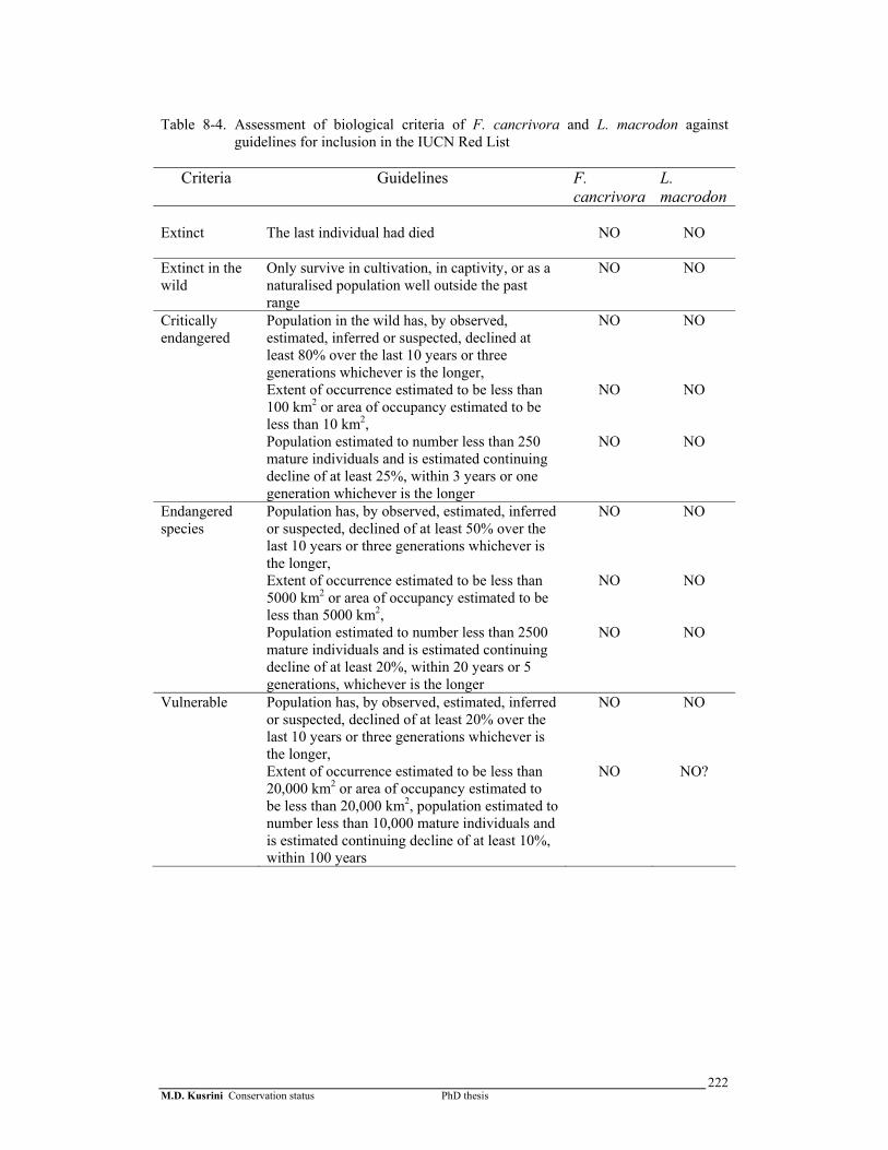
M.D. Kusrini Conservation status PhD thesis
222
Table 8-4. Assessment of biological criteria of F. cancrivora and L. macrodon against
guidelines for inclusion in the IUCN Red List
Criteria Guidelines F. cancrivora
L. macrodon
Extinct
The last individual had died
NO
NO
Extinct in the wild
Only survive in cultivation, in captivity, or as a naturalised population well outside the past range
NO NO
Critically endangered
Population in the wild has, by observed, estimated, inferred or suspected, declined at least 80% over the last 10 years or three generations whichever is the longer,
NO NO
Extent of occurrence estimated to be less than 100 km2 or area of occupancy estimated to be less than 10 km2,
NO NO
Population estimated to number less than 250 mature individuals and is estimated continuing decline of at least 25%, within 3 years or one generation whichever is the longer
NO NO
Endangered species
Population has, by observed, estimated, inferred or suspected, declined of at least 50% over the last 10 years or three generations whichever is the longer,
NO NO
Extent of occurrence estimated to be less than 5000 km2 or area of occupancy estimated to be less than 5000 km2,
NO NO
Population estimated to number less than 2500 mature individuals and is estimated continuing decline of at least 20%, within 20 years or 5 generations, whichever is the longer
NO NO
Vulnerable Population has, by observed, estimated, inferred or suspected, declined of at least 20% over the last 10 years or three generations whichever is the longer,
NO NO
Extent of occurrence estimated to be less than 20,000 km2 or area of occupancy estimated to be less than 20,000 km2, population estimated to number less than 10,000 mature individuals and is estimated continuing decline of at least 10%, within 100 years
NO NO?

M.D. Kusrini Conservation status PhD thesis
223
Table 8-5. Assessment of biological criteria of F. cancrivora and L. macrodon against
guidelines for inclusion in CITES Appendix I Biological Criteria
F. cancrivora L. macrodon
A
The wild population is small and is characterised by at least one of the following
1 An observed, inferred or projected, decline in the number of individuals or area and quality of habitat
NO NO
2 Each population being very small NO NO 3 A majority of individuals, during one or more life-
history phases, being concentrated in one sub-population
NO NO
4 Large short-term fluctuations in the number of individuals
NO NO
5 High vulnerability due to the species biology or behaviour including migration
NO NO
B
The wild population has a restricted area of distribution and is characterized by at least one of the following
1 Fragmented or occurrence at very few locations NO NO 2 Large fluctuation in the area of distribution or the
number of sub-populations NO NO
3 High vulnerability due to the species biology or behaviour including migration
NO NO
4 An observed, inferred or projected decline in area distribution or the number of sub-populations or the number of individuals or area and quality of habitat reproductive potential
NO NO
C
A decline in the number of individuals in the wild which has been either
1 Observed as ongoing or having in the past NO NO 2 Inferred or projected decrease in area or quality of
habitat or levels or pattern of exploitation NO NO
3 Threats from extrinsic factors such as pathogens NO NO 4 Decreasing reproductive potential NO NO D
If the species is not included in Appendix I, it would satisfy with A, B or C period of five years
Recommended status for Appendix I
Not qualified
Not qualified
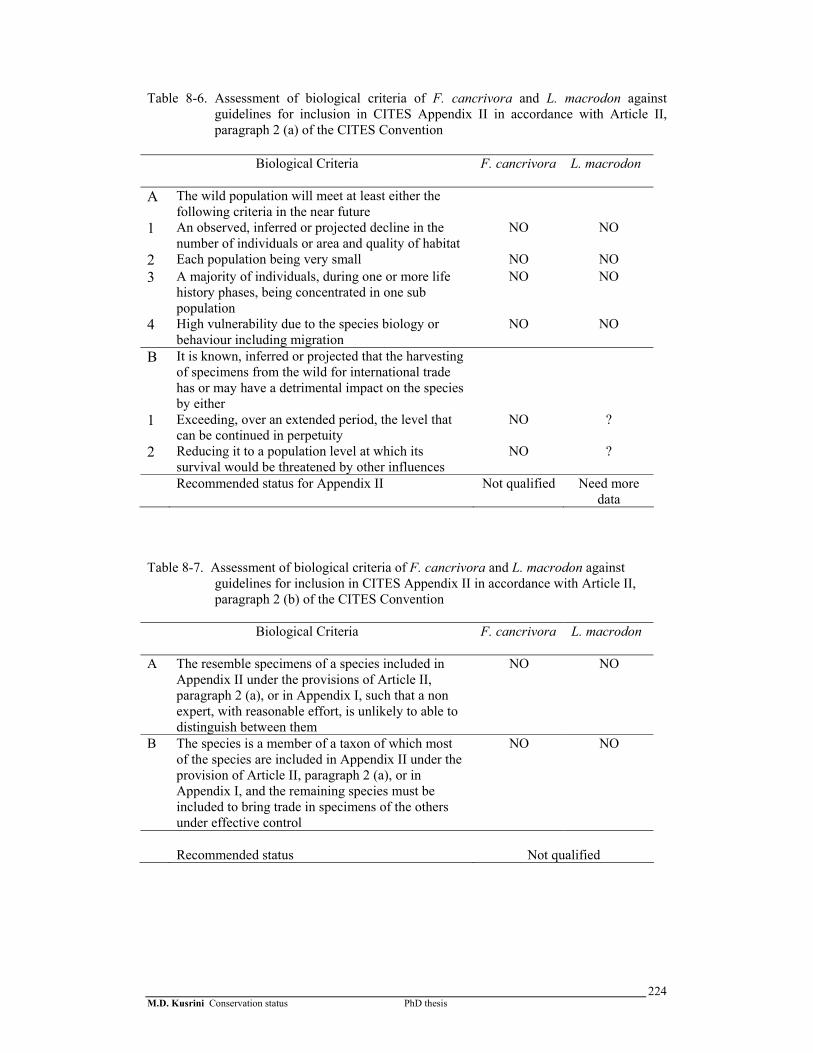
M.D. Kusrini Conservation status PhD thesis
224
Table 8-6. Assessment of biological criteria of F. cancrivora and L. macrodon against guidelines for inclusion in CITES Appendix II in accordance with Article II, paragraph 2 (a) of the CITES Convention
Biological Criteria
F. cancrivora L. macrodon
A The wild population will meet at least either the following criteria in the near future
1 An observed, inferred or projected decline in the number of individuals or area and quality of habitat
NO NO
2 Each population being very small NO NO 3 A majority of individuals, during one or more life
history phases, being concentrated in one sub population
NO NO
4 High vulnerability due to the species biology or behaviour including migration
NO NO
B It is known, inferred or projected that the harvesting of specimens from the wild for international trade has or may have a detrimental impact on the species by either
1 Exceeding, over an extended period, the level that can be continued in perpetuity
NO ?
2 Reducing it to a population level at which its survival would be threatened by other influences
NO ?
Recommended status for Appendix II Not qualified Need more data
Table 8-7. Assessment of biological criteria of F. cancrivora and L. macrodon against
guidelines for inclusion in CITES Appendix II in accordance with Article II, paragraph 2 (b) of the CITES Convention
Biological Criteria
F. cancrivora L. macrodon
A The resemble specimens of a species included in Appendix II under the provisions of Article II, paragraph 2 (a), or in Appendix I, such that a non expert, with reasonable effort, is unlikely to able to distinguish between them
NO NO
B The species is a member of a taxon of which most of the species are included in Appendix II under the provision of Article II, paragraph 2 (a), or in Appendix I, and the remaining species must be included to bring trade in specimens of the others under effective control
NO NO
Recommended status
Not qualified
M.D. Kusrini Conservation status PhD thesis
225
8.4 Discussion
From the simulation exercise, it appears likely that although the level of the
removal of mature F. cancrivora by human harvesting is high, the population can
sustain the harvest. However, the simulation results also show that the number of
frogs currently harvested is probably near the sustainable rate. Any increase in
harvesting, or decrease in the rates of survival and reproduction of frogs due to other
causes, could lead to rapid depletion of populations. Thus, it is high time for the local
authorities to monitor this trade.
Despite the limitations of this model, it still gives a picture of population
trends in relation to harvesting. It is recommended that the model should be
developed, with further study allowing more complete parameterisation and more
accurate estimates of the parameters I was able to include.
My evaluation of the status of F. cancrivora and L. macrodon using the
criteria for the IUCN Red List and CITES Appendices made it clear that F.
cancrivora is not qualified for any listing or inclusion in the appendices. The
distribution of F. cancrivora is from the Malay Peninsula to the Philippines and the
Lesser Sundas as far as Flores; Guangxi and north-eastern coast of Hainan Island,
China; Vietnam (Frost, 2004). In Indonesia, this species is found in almost all major
Indonesian islands including Sumatra, Kalimantan, Java, Bali, Sulawesi and recently
Irian Jaya (the Indonesian part of the island of New Guinea). The distribution of L.
macrodon is also wide, from Burma to Malaya, Thailand and Malaysia; Java and
Sumatra (Indonesia), and the Rioux Archipelago (Frost, 2004). However, in Indonesia
this species is considered endemic in Java, but is also found in Lampung, South
Sumatra (Iskandar, 1998). In Java, it is mostly found in the western part of the island
(Figure 4-4).
M.D. Kusrini Conservation status PhD thesis
226
There are no previous studies of the population status of either species in
Indonesia. My study in West Java indicated that populations of F. cancrivora were
abundant, with a mean density of 40/ha in rice fields. Although concern has been
expressed that this species seems to be hard to find in some rice fields (Pratomo,
1997; Schmuck, 2000), it presently occurs in good population densities at a number of
sites distributed over West Java. Field experience indicates that F. cancrivora can be
difficult to catch and moves actively among rice fields, especially during drying
periods (Chapter 5). This could account for the previous reports of localised declines
in abundance. Wild populations of L. macrodon in my study fluctuated over time,
with a maximum of seven frogs found per 100 m of stream length (Cilember,
December 2002, see Chapter 6). It appears to be common in West Java. The relative
scarcity of information on population status of this species suggests a need for long-
term monitoring to detect possible future declines.
Both F. cancrivora and L. macrodon have high reproductive rates and breed
all year long (Sugiri, 1979; Premo, 1985; Jaafar, 1994, this study). F. cancrivora is
found most abundantly in rice fields rather in than natural habitats such as ponds and
streams. Although rice fields have been a part of the landscape for a sufficient period
that they could be considered a part of the natural environment, their occurrence relies
on human interference. It seems that the frogs have immigrated to rice field areas
naturally and regard rice fields as suitable habitat compared to other habitat. F.
cancrivora has the ability to survive the harsh conditions of rice fields and this ability
has helped this species thrive in the rice fields along with F. limnocharis-iskandari
complex.
Surveys of F. cancrivora in other wetland areas (ponds, streams and marshes)
found no or few individuals (Chapter 4). It appears that by developing large areas of
M.D. Kusrini Conservation status PhD thesis
227
rice fields, humans have probably greatly increased the total abundance of the frog
species that inhabit them. In the past few years, the development of rice fields in
Indonesia has moved towards outer Java and encompasses areas that traditionally had
no rice culture, such as Irian Jaya. The availability of rice fields in other areas has
either allowed an increase in the distribution of F. cancrivora or caused it to increase
in abundance and be detected in new areas; it has only been found in Irian Jaya since
the institution of rice culture there (Chapter 4). L. macrodon is also not restricted to
streams in undisturbed forested areas, and can be found near human habitation
(villages or irrigation channels for rice fields).
Biological criteria for the inclusion of F. cancrivora and L. macrodon in
CITES Appendix II in accordance with Article II, paragraph 2 (b) of the CITES
Convention state that a non-expert with reasonable effort could distinguish between
edible specimens. However, in practicality it is difficult to differentiate both species
by their skinless legs. In its live form mature F. cancrivora can be distinguished from
its sympatric species F. limnocharis-iskandari complex or L. macrodon. However,
non-experts would have difficulty distinguishing L. macrodon with some other
Limnonectes genus such as L. blythii and L. paramacrodon. To date, no Limnonectes
are listed under appendices of CITES.
Should any edible frogs be included in any conservation measures in the
future, the management authorities should account for the fact that it is difficult to
correctly identify (1) species of Limnonectes from live specimens and (2) edible
species from frozen legs as shown by Veith et al., (2000). The first step in managing
the trade is to assure that identification of the frogs is correct. There is a need to
develop a simple key-identification for local authorities and traders, and distribute it,
so they can identify species correctly.

M.D. Kusrini General Discussions & Conclusions PhD thesis
228
CHAPTER 9
GENERAL DISCUSSION AND CONCLUSION
9.1 Introduction
Understanding the Indonesian frog leg harvest requires cross-disciplinary
knowledge, including information on frog biology, population dynamics, and
conservation biology, and an understanding of the human aspects of the harvest. The
literature concerning the species harvested is surprisingly sparse, and much is relatively
old, reaching back more than 20 years. There is more information on the basic biology
(such as diet and breeding biology) of harvested species, but it is mostly found in grey
literature, e.g. unpublished theses, in a language other than English (Bahasa Indonesia).
The results of my study fill gaps in basic understanding of the biology, population
ecology, and conservation biology of edible frogs and their interactions with humans,
and allow me to make recommendations for the conservation of edible frogs, especially
the two most important species: F. cancrivora and L . macrodon.
9.2 The extent of the Indonesian edible frog leg trade
My study is the first to estimate the total number of frogs harvested in Indonesia,
including those harvested for export and for domestic markets. The estimated harvest
for export fluctuates annually, and during the period from 1989 – 1998 was higher than
those of India before the edible frogs of India were listed under CITES (Pandian and
Marian, 1999; Chapter 2). During the last three years for which I had data (1999 – 2002)
the level of frog leg exports declined slightly. This decline does not necessarily indicate
declining harvests, but may reflect a shift from international to domestic markets, or a
reduction in international demand.
M.D. Kusrini General Discussions & Conclusions PhD thesis
229
My study indicated that the harvest for domestic markets is greater than that for
exports (Chapter 3), however, my estimates are subject to uncertainty. They were based
on the ratio of frogs captured by harvesters that had suitable mass for export purposes to
the frogs that were captured but were not suitable for export because they were too
small. Although exporters and middlemen interviewed insisted that frogs exported
should have a minimum weight, the number of exporters and middlemen interviewed in
this study was limited. It is possible that some of the countries that import frog legs are
lowering the criteria, e.g. importing legs from frogs weighing less than 80 grams.
Because of the unregulated nature of this product, the species and sizes of
individuals taken are governed by market demand. Hence, if markets accept smaller
frogs, they will also be harvested. Although harvests occur throughout the year, the rate
of harvesting fluctuates. Peak harvests occur during the wet season and no moon. At a
local scale, frog harvesting in rice fields is also limited by the stage of rice plant growth.
Although access to rice fields is mostly free, harvesters need to take care that their
actions do not damage rice plants; as a result they rarely venture inside rice blocks
except during certain times e.g. after rice is harvested. Thus their capture effort is
usually limited to areas within a one-meter radius of the block borders, which also serve
as pathways. Those limitations may limit the impact of harvesting on frog populations,
since the majority of their habitat is protected from harvesting pressure.
At peak season the number of harvesters tends to rise as part-time harvesters
enter the workforce. Harvesting is not a highly skilled job and provides a substantial
income for unskilled workers. It is evident that frog harvesting in Indonesia, at least in
Java where my study was done, has a long history that predates the first recorded exports
in 1969. It has a large economic value and well-established trading networks. The
number of people involved in this trade is high if we take account full- and part-time

M.D. Kusrini General Discussions & Conclusions PhD thesis
230
harvesters, middlemen, traders, people working in processing plants and export
companies, and people working in restaurants or warung (street vendors) who serve frog
leg delicacies. From my estimates of the total harvest (ca. 400,000,000 frogs per annum)
and harvesting rates (ca. 100 frogs per harvester-day) and length of the working year (ca.
200 days), it is possible to estimate that on the order of 20,000 persons are employed in
frog harvesting in Java. Any regulation of this trade should take account of the
involvement of local people who depend on it for their livelihood.
While my study focused on the trade from Java, the results give an overall
picture of the frog leg trade in Indonesia. Frogs are harvested primarily from rice fields
or areas near human habitations rather than forested areas since frogs are more abundant
in these areas and access is easier. The same trend is probably true for other islands.
My study indicated that currently most harvest for export purposes comes from Java. In
the future, if increased population leads to a decreased area of rice fields in Java, the
harvest for export will probably shift to other islands such as Sumatra, Bali, Kalimantan
and Sulawesi. Even though frog farming has been encouraged by the government, it is
unlikely that frog farming will develop in Indonesia as long as the cost of frogs
harvested in the wild is lower than that of farmed frogs and the species farmed are
considered to be unappetizing by local markets.
9.3 The population dynamics and biology of the harvested species
The population status of the three most common species of edible frogs (F.
limnocharis-iskandari complex, F. cancrivora and L. macrodon) is addressed in
Chapters 5 and 6. My study has provided the first estimates of the densities of F.
limnocharis-iskandari complex and F. cancrivora in Indonesia. My field surveys in
West Java revealed that the mean densities of F. limnocharis-iskandari complex adults
M.D. Kusrini General Discussions & Conclusions PhD thesis
231
and juveniles were 211.76/ha and 514.68/ha, respectively; whilst for F. cancrivora adult
and juveniles they were 39.76/ha and 85.27/ha. The densities of both species in my
study were similar to, and in fact higher than, their densities in Malaysia (Jaafar, 1994).
Given that the locations in my study are subjected to frog harvesting while Jaafar’s
study sites were not, these results suggest that harvesting has not severely depleted the
population of either species.
The population structures of both species differed among rice planting stages;
juveniles were found mostly during tilling and the earlier stages of rice plant growth.
The timing of recruitment of both species is related to water level, an observation also
made by Jaafar et al., (1999) in the rice fields of Malaysia. The ability of the frogs to
breed several times a year (Church, 1960; Jaafar, 1994) has allowed the populations of
both species to flourish despite continuous harvest. Both species showed sexual size
dimorphism, with females larger than males, which causes more females than males to
be captured by harvesters.
Similarly to F. limnocharis-iskandari complex and F. cancrivora, L. macrodon
also showed a tendency for sexual size dimorphism. Although most authors state that
adult males of fanged frogs are larger than females (Inger, 1966; Emerson, 2001) my
study found the opposite: female L. macrodon were larger than males, the same pattern
displayed by the rice field frogs. My study suggests that the minimum reproductive size
for female L. macrodon is approximately 60 mm SVL.
My population estimates for L. macrodon were mostly too variable to be
strongly relied upon, and some mark-recapture parameters could not be estimated at all.
This was caused by low numbers of recaptures of this species, especially at Ciapus
Leutik. The probability of capture differed between capture periods; more frogs were
found during times of higher rainfall than in the dry season. Capture efficiency at
M.D. Kusrini General Discussions & Conclusions PhD thesis
232
Cilember and Ciapus Leutik varied between 0.59 and 0.71; for every two to three frogs
captured, one frog escaped. The density of frogs varied from one per 100m at Ciapus
Leutik to seven per 100 m at Cilember. Although lower numbers of frogs were found at
Ciapus Leutik there is no evidence that this was caused by over-harvesting in the area.
9.4 Environmental stressors
My results suggest that rice field frogs are subject to environmental stressors.
Both F. limnocharis-iskandari complex and F. cancrivora in my study showed signs of
morphological abnormalities, caused both by developmental abnormalities and traumatic
injuries. Although the frequencies of abnormalities in my study were relatively low
compared with results of some other studies (Ouellet, 2000), the results indicate that
stresses may affect the condition of frogs in this habitat.
Pesticide use in agriculture is thought to be a major threat to wildlife (Igbedioh,
1991; Safford and Jones, 1997) including amphibians (Cooke, 1973, 1977 and 1981;
Bridges and Semlitsch, 2000; Hayes et al., 2002; Kiesecker, 2002). The existing
pesticide residues I found reflect a history of substantial use of pesticides by farmers.
Both frog species accumulated pesticides, either through direct contact with the
environment or through ingestion of contaminated prey. Pesticides have been used in
Indonesia for many years (Fox, 1993; Van der Eng, 1994 and Settle et al., 1996), so both
species have been exposed to pesticides for many generations. The relatively high
densities I found for both rice-field species suggest that their population sizes are not
being negatively affected by pesticide exposure. Despite pesticide use, the insects and
other invertebrates the frogs feed upon appear to be abundant in the rice fields (Settle et
al., 1996). Most juveniles found in the survey had good body condition, indicating that
they were not food-stressed.
M.D. Kusrini General Discussions & Conclusions PhD thesis
233
There was no sign of chytridiomycosis in the three species I studied.
Chytridiomycosis has been found infecting many species of frogs around the world
(Berger et al., 1998) and although to date no infection has been found in the species I
surveyed, or in any Indonesian frogs, there is a possibility that this fungus could be
found in other species of Indonesian frogs more susceptible to this disease, or in other
regions or habitats. It is likely that the absence of this disease in Indonesia reflects the
lack of surveys, and since it can cause sudden dramatic collapses of frog populations
(Berger et al, 1998), efforts should be made to gain a greater understanding of its status
in Indonesia.
My analysis of developmental stability determined that in F. limnocharis-
iskandari complex there is a significant excess of fluctuating asymmetry over
measurement error. This indicates that developmental precision was not perfect, which
may have been a reflection of environmental stress. However, I was not able to
determine whether any particular stress might have been the cause of the observed levels
of fluctuating asymmetry. I did not find any significant differences of fluctuating
asymmetry between frogs captured in pesticide and non-pesticide locations (Chapter 9),
however I also found no major differences in pesticide levels in the environment or in
frogs between these sites. More importantly, I found no correlation between body
condition and level of unsigned asymmetry in individuals. Body condition, however,
was correlated with environmental conditions, being lower in the relative drought
experienced in 2003. My results suggest that at least in the species studied,
developmental stability analysis is not a powerful tool to detect short-term stress (e.g.
the impact of drought).
M.D. Kusrini General Discussions & Conclusions PhD thesis
234
9.5 The sustainability of harvest and conservation status of the edible frogs
The attitudes revealed in my surveys of people involved in the frog-leg trade
indicate that most traders are not overly concerned with the conservation of the edible
species. Although some harvesters and middlemen expressed concern at low harvest
rates, there is a general belief among the stakeholders that the harvest can sustain trade
for an unlimited time. There is also almost no political will to regulate the trade.
Working out which government agencies are responsible for the trade is complicated.
For instance, in statistical data frog legs were listed as fisheries commodities and thus
are under the jurisdiction of the Ministry of Marine Affairs and Fisheries. The Ministry
of Marine Affairs and Fisheries itself is a young department, which developed from a
directorate general under the Ministry of Agriculture. When my study began, the frog
harvest, which is considered to be an inland fishery, was still under the jurisdiction of
the Ministry of Agriculture. Later, with reorganization of the government departments, it
was moved into the Ministry of Marine Affairs and Fisheries. However, the frog leg
trade is not the main focus of this Ministry, compared with other commodities such as
prawns, tuna or other marine fisheries. Exporting frog legs also involves the Provincial
Office of Industry and Trade.
The export of Indonesian wildlife in particular has resulted in the decline of some
species and has been closely monitored by the international public (Soehartono and
Mardiastuti, 2002). To answer the problem, the Government of Indonesia developed a
conservation strategy to promote the protection of life support systems, preservation of
genetic resources and sustainable utilization of living resources. The Government of
Indonesia ratified the CITES Convention through Presidential Decree No 43 in 1978
(Soehartono & Maridastuti, 2002) and later on promulgated a ministerial decree from the

M.D. Kusrini General Discussions & Conclusions PhD thesis
235
Ministry of Forestry regulating the capture, transport and trade of wild flora and fauna
(PHPA, 1990).
For the implementation of CITES, the Government of Indonesia designated the
Directorate General of Forest Protection and Nature Conservation (Direktorat Jenderal
Perlindungan Hutan dan Konservasi Alam, PHKA) as the management authority and
The Indonesian Institute of Science (Lembaga Ilmu Pengetahuan Indonesia, LIPI) as the
scientific authority. The latter is responsible for advising PKA on the status of species
subjected to harvest for international trade, whilst the former establishes the annual
harvest quota. As Indonesia has become one of the major exporters of frog legs in the
world (Chapter 2), and it is well known that the exported frogs are mostly wild-caught,
it is not surprising that the Indonesian frog harvest has also been questioned by
international investigations (Barfield, 1986; Niekisch, 1986; Martens, 1991; Patel, 1993;
Schmuck, 2000). Although no Indonesian frog species has been included in the CITES
convention, the PKA does set a quota for this harvest as part of an attempt to regulate
the harvest of wildlife of non protected and non-CITES species. For instance, the annual
quota in 2001 is 5,000 F. cancrivora for pets and 25,000 L. macrodon for skins plus
additional 5,000 for pets (PKA, 2000).
The establishment of annual quotas of F. cancrivora and L. macrodon by the
PKA showed the absurdity of the situation. It is clear from my results that millions of
these species are caught annually to satisfy the international and domestic demands of
the food industry. The PKA quotas did not acknowledge the harvest for food. Also if the
number of frogs harvested is reduced to the number established by the PKA, the frog
harvesting industry will cease to exist. From the stand point of law, the exclusion of
edible species from protected species means that there are no legal issues in harvesting

M.D. Kusrini General Discussions & Conclusions PhD thesis
236
these species, which is probably the reason why the annual quota put by the PKA has no
influence whatsoever on the actual harvest of frogs in the wild.
Attempts to regulate the harvest of frog legs will be impossible without
acknowledging the already established market for frog legs and the stakeholders
involved in this industry. Even if an export quota were set, controlling the domestic
market will be complicated and most likely will not succeed. The majority of harvesters
are uneducated and poor and will not accept quotas or acquiesce if the practice of
harvesting frogs, which has provided livelihoods for many years and is not objected to
by most rice field owners, is stopped by the government. Harvesting occurs on almost
all Indonesian islands, making law enforcement difficult. Any restrictions on the
harvest, as have been attempted by the PKA, require a detailed knowledge of the status
and dynamics of populations of the harvested species.
As stated before, the scientific authority responsible for CITES in Indonesia is
LIPI. However, LIPI has limited resources for monitoring harvested species (Amir et al,
1998). There is a need for LIPI to develop greater cooperation with other scientific
organizations (such as universities) and non-governmental organizations to monitor
these species. Collaboration with professional bodies such as IRATA (the Indonesian
Reptile and Amphibian Trader Association) to monitor the harvest of several species of
reptiles is one of the examples of cooperation already operating (Saputra, 1998). In the
case of frog legs, there are no reports of attempts by any professional body to survey the
level of the frog harvest. Although the name of IRATA suggests the inclusion of
amphibian traders in this professional body, it does not include the frog leg industry;
only the live amphibian trade for the pet industry (Saputra, pers. comm.). The
organization that deals with the frog leg industry is most likely included in the Cold

M.D. Kusrini General Discussions & Conclusions PhD thesis
237
Storage & Fisheries Commodities Trader Association (Asosiasi Pengusaha Cold
Storage dan Produsen Exportir Hasil Perikanan Indonesia; APCI).
Although the estimated numbers of frogs harvested annually in Indonesia are
huge (Chapter 2 & 3) there is no evidence that the harvest has depleted the populations
of rice field frogs. However, the present level of harvest of F. cancrivora may be near
the maximum level sustainable by the population, as indicated by the results of my
modelling (Chapter 8) and by the fact that the population structure of F. cancrivora in
the field was mostly biased to young mature frogs (Chapter 5) when compared with
unharvested populations that have been studied elsewhere.
Fieldwork showed that F. limnocharis-iskandari complex were found in high
abundances (Chapter 5). The densities of F. cancrivora populations were also high
(Chapter 5), and (Chapter 8) it did not meet any criteria for listing as a protected
species. Modelling and assessment of F. cancrivora using the IUCN Red List and
CITES criteria also showed that it does not qualify for any inclusion, as long as the level
of harvesting and habitat size remain constant. The conclusion that both Indonesian rice
field frogs’ populations appear to be able to sustain the relatively high rates of harvest
they are experiencing differs from the conclusions reached in research on Indian edible
frogs (Abdulali, 1985) that resulted in the inclusion of Euphyctis hexadactylus and
Holobatrachus tigerinus in CITES Appendix 2. My results are similar to those found in
a series of studies on the harvest of pythons and monitors in Indonesia during late
1990’s (Shine et al., 1996; Boeadi et al., 1998; Shine et al., 1998a, 1998b, 1998c,
1998d, 1998e, and 1998f). These studies showed that the populations of harvested
species have been able to withstand continuous harvest pressure due to their life history
traits including rapid growth, early maturation, and relatively high reproductive output
and also their ability to thrive in disturbed landscapes.
M.D. Kusrini General Discussions & Conclusions PhD thesis
238
Assessment of L. macrodon in the market and fields showed that this species is
still considered abundant, especially in the western part of Java. However, there is a
need for more studies to assess the status of this species. It occurred at relatively low
densities, and I did not collect sufficient data on either harvesting rates or population
parameters to allow a full evaluation of the sustainability of its harvest.
9.6 Conclusions and Recommendations
My study suggests that the current levels of harvest of F. cancrivora and F.
limnocharis-iskandari complex are sustainable. The impact of harvesting on L.
macrodon is unclear. Current levels of harvest appear likely to affect L. macrodon
populations more than F. cancrivora, however, there is a need to do more research on
the population biology and ecology of this species.
Although I conclude that there is no justification for including the harvested
species in the Red List or in the CITES appendices, the scientific authority (LIPI)
should regularly monitor the trade. Monitoring of the frog leg trade should occur not
only in Java but also in the other main islands, especially Sumatra. From the export
statistics, the centre of exportation in Sumatra is in Medan, thus the monitoring in
Sumatra should begin from Medan and surrounding North Sumatran areas. Monitoring
should include collection of data on species harvested, size harvested, the spatial and
temporal patterns of harvest, and the population ecology of the species harvested.
Because of the potential economic gain from this harvest, especially for export
purposes, the government (e.g. the ministry of fisheries and marine affairs) should also
monitor this harvest. Monitoring the harvesters itself might prove difficult due to the
open nature of this work. One way to trace the number of people involved in this export
might be through the export companies. All export companies maintain strong

M.D. Kusrini General Discussions & Conclusions PhD thesis
239
relationship with their middleman, and middleman with their harvesters. The
government should monitor the numbers of export companies and their middleman and
regularly update it.
Another concern regarding this trade is incorrect species identifications in export
documents. With enough effort, species identification is not difficult to do while the
frog is still alive. On the other hand, identifying species from frozen leg is likely to
require the use of molecular genetics, which is costly. Therefore there is a need for local
trade officials to impose correct species identification on the middleman levels.
Developing a simple identification key and distributing it to the middlemen thorough
exporting companies would be the first step to ensure correct identifications.
There is a need to assess the possibility of farming local frogs for this trade. If it
proved successful and cost-efficient, local frogs farming could replace the farming of
the exotic species Rana catesbeiana, which has become established as an exotic and
threatened native fauna in other places where it has been introduced for farming.
In conclusion, the Indonesian frog leg trade employs a large number of people
and is an important sector of the economy. There is presently no evidence that
harvesting is being conducted at unsustainable levels, and therefore there does not seem
to be any conservation need to reduce the rate of harvesting. There is a need to
improve the quality and quantity of information available on the industry, and our
understanding of the biology of the species harvested, so that developing problems can
be averted before they become serious. There is also a need to ensure that harvesting is
limited to species that are not adversely impacted.
M.D. Kusrini References PhD thesis
240
REFERENCES Abdullah, A. R. 1991. Persistent organochloride pesticides in the tropical environment. Wallaceana 64: 1-6. Abdulali, H. 1985. On the export of frog legs from India. J. Bombay Nat. Hist. Soc. 2: 347-375. Achmad and F. G. Sulaiman. 2000. Monyet dan beruk sebagai komoditi ekspor dan peluangnya dalam bisnis di Indonesia. Prosiding Seminar Primatologi Indonesia, Yokyakarta.. p: 52-66 Akita, T. and A. Alisjahbana. 2002. Regional income inequality in Indonesia and the initial impact of the economic crisis. Bulletin of Indonesian Economic Studies 38(2): 201-222. Alcala, A. C. 1962. Breeding behaviour and early development of frogs of Negros, Philippine islands. Copeia 1962 (4): 679 - 726. Alexander, P. S., C. M. Chang and C. H. Yang. 1963. Reproductive variation in the female rice frog Rana limnocharis during the spring season in Taiwan. Biological Bulletin Tunghai University 20: 1-4. Alexander, P. S., A. C. Alcala and D. Y. Wu. 1979. Annual reproductive pattern in the rice frog Rana l.limnocharis in Taiwan. Journal of Asian Ecology 1979 (1): 68-78. Alford, R., K. Bradfield and S. Richards. 1999. Measuring and analysing developmental instability as a tool for monitoring frog populations. In: A. Campbell (eds) Declines and dissapearances of australian frogs. Canberra, Environment Australia: 34-43 pp. Alford, R. A. and S. J. Richards. 1999. Global amphibian declines: A problem in applied ecology. Ann.Rev. Ecol. Syst. 30: 133-165. Anonymous. 1991. Declining amphibian populations - a global phenomenon? Findings and recommendation. Workshop on declining amphibian population on 19-20 February 1990. Alytes 9 (2): 33-42. Ardiwinata, A. N., J. Soejitno, E. S. Harsanti, H. Purwanti and S. Y. Jatmiko. 2001. Jenis dan kelimpahan biota di ekosistem tanaman pangan. Jakenan, Pati, Jawa Tengah, Loka Penelitian Tanaman Pangan: 13 pp. Arie, U. 1999. Pembibitan dan pembesaran bullfrog. Jakarta, Penebar Swadaya.104 pp. Atmowidjojo, A. H. and Boeadi. 1988. Food prey on the stomach content of frogs. Biotrop Spec. Publ. 32: 77-80. Ayas, Z., N. E. Barlas and D. Kolankaya. 1997. Determination of organochlorine pesticide residues in various environments and organisms in Giiksu delta, turkey. Aquatic Toxicology 39 (1997): 171-181.
M.D. Kusrini References PhD thesis
241
Baird, R. W., A. M. Gorgone, A. D. Ligon and S. K. Hooker. 2001. Mark-recapture abundance estimate of bottlenose dolphins (Tursiops truncatusi) around Maui and Lana'i, Hawai'i during the winter of 200/2001. Report. La Jolla, Southwest Fisheries Science center, National Marine Fisheries Service USA. Barbier, E. B., J. C. Burgess, T. M. Swanson and D. W. Pearce. 1990. Elephants, economics and ivory. First Edition. London, Earthscan Publication Ltd.154 pp. Barfield, S. 1986. Indonesia's frog legs. Journal of Environmental Health 48 (6): 324. Barinaga, M. 1990. Where have all the froggies gone? Science 247: 1033-1034. Beebee, T. J. C. 1996. Ecology and conservation of amphibians. London, Chapman & Hall.214 pp. Beissinger, S. R. and E. H. Bucher. 1992. Can parrots be conserved through sustainable harvesting? Bioscience 42 (3): 164-174. Bennett, D. 2000. The density and abundance of juvenile Varanus exanthematicus (Sauria: Varanidae) in the coastal plain of Ghana. Amphibia-Reptilia 21 (3): 301-306 Berger, L., R. Speare, P. Daszak, D. E. Green, A. A. Cunningham, C. L. Goggin, R. Stratcombe, M. A. Ragan, A. D. Hyatt, K. R. McDonald, H. B. Hines, K. R. Lips, G. Farantelli and H. Parkes. 1998. Chytridiomycosis causes amphibian mortality associated with population declines in the rain forest of Australia and Central America. Proc.Natl.Acad.Sci. USA 95: 9031-9036. Berger, L., R. Speare and A. Hyatt. 1999. Chytrid fungi and amphibian declines: Overview, implications and future directions.In: A. Campbell (eds) Declines and disappearances of Australian frogs. Canberra, Environment Australia: 23-33 pp. Berger, L., R. Speare, H. Hines, G. Marantelli, A. Hyatt, K. McDonald, L. Skerratt, V. Olsen, J. Clarke, G. Gillespie, M. Mahony, N. Sheppard, C. Williams and M. J. Tyler. 2004. Effect of season and temperature on mortality in amphibians due to chytridiomycosis. Australian Veterinary Journal 82: 31-36. Berger, L., R. Speare and A. Kent. 2000. Diagnosis of chytridimicosis in amphibians by histologic examination. Zoo’s Print Journal XV (1): 184-190. Berrill, M., D. Coulson, L. Mcgillivray and B. Pauli. 1998. Toxicity of endosulfan to aquatic stages of anuran amphibians. Environmental Toxicology & Chemistry 17 (1): 1738-1744. Berry, P. Y. 1964. The breeding patterns of seven species of Singapore anura. J. Anim. Ecol. 33: 227-243. Berry, P. Y. 1975. The amphibian fauna of Peninsular Malaysia. Kuala Lumpur, Tropical Press.127 p.
M.D. Kusrini References PhD thesis
242
Beshkov, V. A. and D. L. Jameson. 1980. Movement and abundance of the yellow-bellied toad Bombina variegata. Herpetologica 36 (4): 365-370. Beverton, R. 1998. Fish, fact and fantasy: A long view. Reviews in Fish Biology and Fisheries 8: 229-249. Bjorksten, T., P. David, A. Pomiankowski and K. Fowler. 2000. Fluctuating asymmetry of sexual and nonsexual traits in stalk-eyed flies: A poor indicator of developmental stress and genetic quality. Journal of Evolutionary Biology 13 (1): 89-97. Blaustein, A. R. 1994. Chicken little or Nero’s fiddle? A perspective on declining amphibian populations. Herpetologica 50 (1): 58-97. Blaustein, A. R. and D. B. Wake. 1990. Declining amphibian population: A global phenomenon? Trends in Ecology and Evolution 5 (7): 203-204. Blaustein, A. R. and D. B. Wake. 1995. The puzzle of declining amphibian population. Scientific American: 56-61. Blaustein, A. R., D. P. Wake and W. P. Sousa. 1994. Amphibian declines: Judging stability, persistence, and susceptibility of populations to local and global extinctions. Conservation Biology 8 (1): 60-71. Boeadi, R. Shine, Sugardjito, M. Amir and M. H. Sinaga. 1998. Biology of the commercially-harvested ratsnake (Ptyas mucosus) and cobra (Naja sputatrix) in Central Java. Mertensiella 9 :99-104. Boyden, S. 1992. Biohystory: The interplay between human society and the biosphere - past and present. Paris, UNESCO.265 pp Boone, M. D. and R. D. Semlitsch. 2001. Interactions of an insecticide with larval density and predation in experimental amphibian communities. Conservation Biology 15 (1): 228-238. BPS. 1969 – 2003. Statistik Perdagangan luar negeri Indonesia (Indonesian foreign trade statistics) Vol I & II. Biro Pusat Statistik Indonesia, Jakarta.
BPS, 2000. Survey Pertanian : Luas Lahan Menurut Penggunaannya di Jawa Agricultural Survey Land Area by Utilization in Java. Biro Pusat Statistik, Jakarta.
BPS. 2002. Statistik Kesejahteraan Rakyat : Survey Sosial Ekonomi Nasional. Biro Pusat Statistik, Jakarta.
BPS. 2002. Statistik Kesejahteraan Rakyat : Survey Sosial Ekonomi Nasional. Biro Pusat Statistik, Jakarta.
Bridges, C. M. and R. D. Semlitsch. 2000. Variation in pesticide tolerance of tadpoles among and within species of Ranidae and patterns of amphibian decline. Conservation Biology 14 (5): 1490-1499.

M.D. Kusrini References PhD thesis
243
BrÖnmark, C. and P. Edenham. 1994. Does the presence of fish affect the distribution of tree frogs (Hyla arborea)? Conservation Biology 8(3): 841-845. Brooks, J. A. 1981. Otolith abnormalities in Limnodynastes tasmaniensis tadpoles after embrionic exposure to the pesticide dieldrin. Environmental Pollution Series A 25: 19-25. Bruckner, A. W. 2000. New threat to coral reefs: Trade in coral organisms. Issues in Science and Technology. Fall 2000: 63-68. Cade, B.S, and J. Richards, 1999, User Manual for Blossom Statistical Software: Fort Collins, CO, U.S. Geological Survey, 107 pp. Cairns, S. C. and R. T. Kingsford. 1995. Harvesting wildlife: Kangaroos and waterfowl.In: R. A. Bradstock, T. D. Auld, D. A. Keith et al. (eds) Conserving biodiversity: Threats and solutions, Surrey Beatty & Sons: 260-272. Callister, D. J. and L. M. Williams. 1995. Australia's native wildlife trade: Scale, trends and impacts.In: R. A. Bradstock, T. D. Auld, D. A. Keith et al. (eds) Conserving biodiversity: Threats and solutions., Surrey Beatty & Sons.: 273-291. Carey, C. 1993. Hypothesis concerning the causes of the disappearance of boreal toads from the mountain of Colorado. Conservation Biology 7 (2): 355-362. Carey, C. and C. J. Bryant. 1995. Possible interrelations among environmental toxicants, amphibian development, and decline of amphibian populations. Environmental Health Perspective 103 (Suppl 4): 13-17. Carson, R. 1962. Silent spring. New York, Houghton Mifflin Company.297 pp. Caughley, G. 1977. Analysis of vertebrate populations. New York, John Wiley and Sons.234 pp. Chi, H. 2000. Computer simulation models for sustainability. International Journal of Sustainability in Higher Education 1 (2): 154-167. Church, G. 1960. The effects of seasonal and lunar changes on the breeding pattern of the edible Javanese frog, Rana cancrivora Gravenhorst. Treubia 25 (2): 215-233. Clarke, R. D. 1972. The effect of toe clipping on survival in fowler's toad (bufo woodhouse fowleri). Copeia 1972 (1): 182-185. Clarke, G. M. 1994. Developmental stability analysis: An early warning system for biological monitoring of water quality. Australian Biologist 7 (2): 94-104. Clayton, L. and E. J. Milner-Gulland. 2000. The trade in wildlife in north Sulawesi, Indonesia. In: J. G. Robinson and E. L. Bennett (eds) Hunting for sustainability in tropical forests. New York, Columbia University Press: 473 - 496.

M.D. Kusrini References PhD thesis
244
Clayton, L., M. Keeling and E. J. Milner-Gulland. 1997. Bringing home the bacon: A spatial model of wild pig hunting in Sulawesi, Indonesia. Ecological Application 7 (2): 642-652. Cloudsley-thompson, J. L. 1999. The diversity of amphibians and reptiles: An introduction. Berlin, Springer-Verlag.254 pp. Cohen, M. M. J. 2001. Is Kermit the frog in trouble? American Journal of Medical Genetics 104: 99-100. Cooke, A. S. 1970. The effect of pp'-ddt on tadpoles of the common frog (Rana temporaria). Environmental Pollution 1: 57-71. Cooke, A. S. 1973. The effects of DDT, when used as a mosquito larvacide, on tadpoles of the frog Rana temporaria. Environmental Pollution 5: 259-273. Cooke, A. S. 1977. Effects of field applications of the herbicides diquat and dichlobenil of amphibians. Environmental Pollution Series A 12: 43-50. Cooke, A. S. 1981. Tadpoles as indicators of harmful levels of pollution in the field. Environmental Pollution Series A 25: 123-133. Dash, M. C. and J. K. Mahanta. 1993. Quantitative analysis of the community structure of tropical amphibian assemblages and its significance to conservation. J. Biosci. 18 (1): 121-139. Daszak, P., L. Berger, A. A. Cunningham, A. D. Hyatt, D. E. Green and R. Speare. 1999. Emerging infectious diseases and amphibian population declines. Emerging Infectious Diseases 5 (6): 735-748. Directorate General of Fisheries (DGF). 2001. Program peningkatan eskpor hasil perikanan 2003 . Jakarta, Indonesia. Duellman, W. E. and L. Trueb. 1994. Biology of amphibian. Baltimore, The Johns Hopkins University Press.670 pp. Dunson, W. A. 1977. Tolerance to high temperature and salinity by tadpoles of the Phillipine frog, Rana cancrivora. Copeia 1997: 375-378. Dole, J. W. and P. Durant. 1974. Movements and seasonal activity of Atelopus oxyrhynchus (anura: Atelopodidae) in a Venezuelan cloud forest. Copeia 1974 (1): 230-235. Dyson, M. L., S. P. Henzi, T. R. Halliday and L. Barrett. 1998. Success breeds success in mating male reed frogs (Hyperolius marmoratus). Proc. Roy. Soc. Lond. B. 265: 1417–21. Ecobichon, D. J. 2001. Pesticide use in developing countries. Toxicology 160 (2001): 27–33.
M.D. Kusrini References PhD thesis
245
Emerson, S. B. 2001. A macroevolutionary study of historical contingency in the fanged frogs of Southeast Asia. Biological Journal of the Linnean Society 73: 139–151. Emerson, S. 1992. Courtship and nest-building behavior of a Bornean frog, Rana blythi. Copeia 1992(4): 1123-1127. Emerson, S. B., C. N. Rowsemitt and D. L. Hess. 1993. Androgen levels in a Bornean voiceless frog, Rana blythi. Can. J. Zool. 71: 196-203. Emerson, S. B. and R. F. Inger. 1992. The comparative ecology of voiced and voiceless Bornean frogs. Journal of Herpetology 26 (4): 482-490. Emerson, S. B. and R. Ward. 1998. Male secondary sexual characteristics, sexual selection, and molecular divergence in fanged Ranid frogs of Southeast Asia. Zoological Journal of the Linnean Society 122: 537–553. Erdelen, W., Ed. 1998. Conservation, trade and sustainable use of lizards and snakes in Indonesia. Mertensiella 7. Rheinbach, Germany. Favre, D. S. 1985. International trade in endangered species: A guide to CITES. The Netherlands, Martinus Nijhoff Pub.415 p. Felton, A. 1999. Determinants of male mating success in the microhylid frog, Cophixalus ornatus. Bachelor of Science Honours Thesis. The Department of Zoology and Tropical Ecology, James Cook University. Townsville. 71 pp. Fitter, R. 1986. Wildlife for man: How and why we should conserve our species. First edition. London, Collins.223 pp. Fox, J. J. 1993. Ecological policies for sustaining high production in rice: Observations on rice intensification in Indonesia. In: H. Brookfield and Y. Byron (eds) South-east Asia’s environmental future: The search for sustainability. Kuala Lumpur, Oxford University Press: 211-241 pp. Freese, C. H. 1998. Wild species as commodities: Managing market and ecosystems for sustainability. Washington, Island Press.319 pp. Friedl, T. W. P. and G. M. Klump. 1997. Some aspects of population biology in the European treefrog, hyla arborea. Herpetologica 53 (3): 321-330. Frost, D. R. 1985. Amphibian species of the world: A taxonomic and geographical reference. USA, Allen Press.732 pp. Frost, D.l R. 2004. Amphibian Species of the World: an Online Reference. Version 3.0 (22 August, 2004). Electronic Database accessible at http://research.amnh.org/herpetology/amphibia/index.php. American Museum of Natural History, New York, USA.
M.D. Kusrini References PhD thesis
246
Gibbons, J. W., D. E. Scott, T. J. Ryan, K. A. Buhlmann, T. D. Tuberville, B. S. Metts, J. L. Greene, T. Mills, Y. Leiden, S. Poppy and C. Winne. 2000. The global decline of reptiles, deja vu amphibians. 2000. BioScience 50 (8):653-666. Gillespie, G. R. 2001. The role of introduced trout in the decline of spotted tree frog (Litoria spenceri) in south-eastern Australia. Biological Conservation 100 (2001): 187-198. Gillilland, C., C. Summer, M. Gillilland, K. Kannan, D. Villeneuve, K. Coady, P. Muzzall, C. Mehne and J. Giesy. 2001. Organochlorine insecticides, polychlorinated biphenyls, and metals in water, sediment, and green frogs from southwestern michigan. Chemosphere 44 (3): 327-339. Ginoga, L. N. 1999. Pencemaran insektisida pada tiga spesies burung air di areal persawahan Sukamandi, Subang, Jawa Barat. MSc. Thesis. Pascasarjana, Insitut Pertanian Bogor, Bogor. 95 pp. Golay, N. and H. Durrer. 1994. Inflammation due to toe-clipping in natterjack toads (Bufo calamita). Amphibia-Reptilia 15: 81-83. Gorzula, S. 1996. The trade in dendrobatid frogs from 1986 to 1993. Herpetological Review 27(3): 116-123. Halliday, T. R. and P. A. Verrell. 1988. Body size and age in amphibians and reptiles. Journal of Herpetology 22 (3): 253-265. Hayes, T., A. Collins, M. Lee, M. Mendoza, N. Noriega, A. Stuart and A. Vonk. 2002. Hermaphroditic, demasculinized frogs after exposure to the herbicide atrazine at low ecologically relevant doses. Proc Natl Acad Sci U S A 99 (8): 5476-80. Hayes, M. P. and M. R. Jennings. 1986. Decline of ranid frog species in western North America: Are bullfrogs (Rana catesbiana) responsible? Journal of Herpetology 20: 490 - 509. Helgen, J., R. G. McKinnell and M. C. Gernes. 1998. Investigation of malformed northern leopard frogs in Minnesota. In: M. J. Lannoo (eds) Status and conservation of Midwestern amphibians. Iowa, University of Iowa Press: 288-297.. Hero, J. 1989. A simple code for toe clipping anurans. Herp Review 20 (3): 66-67. Heying, H. E. 2001. Social and reproductive behaviour in the Madagascan poison frog, Mantella laevigata, with comparisons to the dendrobatids. Anim. Behav. 61: 567-577. Hofrichter, R. E. 2000. The encyclopedia of amphibians. Ontario, Key Porter Books Lim.215 pp. Hurtado-Gonzales, J. L. and R. E. Bodmer. 2004. Assessing the sustainability of brocket deer hunting in the Tamshiyacu-tahuayo communal reserve, northeastern Peru. Biological Conservation 116 (2004): 1-7.
M.D. Kusrini References PhD thesis
247
Hutchings, J. A. 2001. Conservation biology of marine fishes: Perceptions and caveats regarding assignment of extinction risk. Can. J. Fish. Aquat. Sci. 58: 108–121. Hutton, J. and B. Dickson. 2000. Endangered species threatened convention: The past, present and future of CITES. London, Earthscan Publication Ltd.202 pp. Igbedioh, S. O. 1991. Effects of agricultural pesticides on humans, animals, and higher plants in developing countries. Archives of Environmental Health 46 (4): 218-224. Inger, R. F. 1966. The systematics and zoogeography of the amphibia of Borneo. Chicago, Field Museum of Natural History.402 pp. Iskandar, D. T. 1998. Amfibi Jawa dan Bali. Bogor, Puslitbang Biologi-LIPI.132 p. Iskandar, D. T. and E. Colijn. 2000. Preliminary checklist of Southeast Asian and New Guinean herpetofauna: I. Amphibians. Treubia 31 (3 Supplement): 1-133. Jaafar, I. H. 1994. The life history, population and feeding biology of two paddy field frogs, Rana cancrivora gravenhorst and R. limnocharis boie, in Malaysia. Doctor of Philosophy Thesis. Faculty of Science and Environmental Studies, University Pertanian Malaysia, Malaysia. 228 pp. Jaafar, I. H., A. Ismail and A. Kurais. 1999. Correlations of reproductive parameters of two tropical frogs from Malaysia. Asiatic Herpetological Research 8: 48-52. Jaafar, I., A. Ektella, M. Mansor and S. Shahrudin. 2002. A comparative study of the amphibian community at three sites in Penang state, Malaysia. FROGLOG 50. Jackson, J. B. C., M. X. Kirby, W. H. Berger, K. A. Bjorndal, L. W. Botsford, B. J. Bourque, R. H. Bradbury, R. Cooke, J. Erlandson, J. A. Estes, T. P. Hughes, S. Kidwell, C. B. Lange, H. S. Lenihan, J. M. Pandolfi, C. H. Peterson, R. S. Steneck, M. J. Tegner and R. R. Warner. 2001. Historical overfishing and the recent collapse of coastal ecosystems. Science 293: 269-638. Jeffers, J. N. R. 1978. An introduction to system analysis: With ecological applications., University Park Press. Jenkins, M. D. 1995. Tortoises and freshwater turtles: The trade in Southeast Asia. Traffic International.48 pp. Jennings, M. R. and M. P. Hayes. 1985. Pre-1900 overharvest of California red-legged frogs (Rana aurora draytonii): The inducement for bullfrog (Rana catesbiana) introduction. Herpetologica 41: 94-103. Jocelyn, K. 1999. Link to parasites grows stronger. Science 286 (5449): 2434. Johnson, P. T. J., K. B. Lunde, E. G. Ritchie, J. K. Reaser and A. E. Launer. 2001. Morphological abnormality patterns in a Californian amphibian community. Herpetologica 57 (3): 336-352.
M.D. Kusrini References PhD thesis
248
Kaiser, J. 1999. A trematode parasite causes some frog deformities. Science 284: 731-732. Kam, Y. C., T. C. Chen, J. T. Yang, F. C. Yu and K. M. Yu. 1998. Seasonal activity, reproduction, and diet of a riparian frog (Rana swinhoana) from a subtropical forest in Taiwan. Journal of Herpetology 32 (3): 447-452. Kellner, J. R. and R. A. Alford. 2003. The ontogeny of fluctuating asymmetry. The American Naturalist 161 (6): 931-947. Kiesecker, J. M. 2002. Synergism between trematode infection and pesticide exposure: A link to amphibian limb deformities in nature? PNAS 99 (15): 9900–9904. Krebs, C. J. 1999. Ecological methodology. 2nd Edition. California, Addison Weley Longman, Inc.620 pp. Kumbar, S. M. and K. Pancharatna. 2001. Occurrence of growth marks in the cross section of phalanges and long bones of limbs in tropical anurans. Herpetological Review 32 (3): 165-167. Lau, A. S. M. and D. S. Melville. 1994. International trade in swiftlet nests with special reference to Hong Kong, Traffic International: 35 pp. Lamont, B. B., R. MArsula, N. J. Enright and E. T. F. Witkoski. 2001. Conservation requirements of an exploited wildflower: Modelling the effects of plant age, growing conditions and harvesting intensity. Biological Conservation 99: 157-168. Lanoo, M. J., K. Lang, T. Waltz and G. S. Phillips. 1994. An altered amphibian assemblage: Dickinson county, Iowa, seventy years after Frank Blanchard's survey. American Midland Naturalist 131: 311-319. Lawler, S. P., D. Dritz, T. Strange and M. Holyoak. 1999. Effects of introduced mosquito fish and bullfrogs on the threatened California red-legged frog. Conservation Biology 13 (3): 613-622. Lee, R. J. 2000. Impact of subsistence hunting in north Sulawesi, Indonesia and conservation options. In: J. G. Robinson and E. L. Bennett (eds) Hunting for sustainability in tropical forest. New York, Columbia University Press: 455-472. Lemckert, F. and T. Brassil. 2000. Movements and habitat use of the endangered giant barred river frog (Mixophyes iteratus) and the implications for its conservation in timber production forests. Biological Conservation 96 (2000): 177-184. Leong, T. M. 2001. Parasitic copepods responsible for limb abnormalities. Froglog 46 (3). Liem, D. S. S. 1971. The frogs and toads of Tjibodas national park Mt. Gede, Java, Indonesia. The Philippine Journal of Science 100 (2): 131-161.
M.D. Kusrini References PhD thesis
249
Lima, A. P., W. E. Magnusson and D. G. Williams. 2000. Differences in diet among frogs and lizards coexisting in subtropical forests of Australia. Journal of Herpetology 34 (1): 40-46. Lips, K. R. 1998. Decline of a tropical montane amphibian fauna. Conservation Biology 12 (1): 106-117. Martens, H. 1991. Trade in frog legs of wild SE Asian Rana species: Some facts and considerations. Germany, Scientific Authorities of CITES, Germany. Martin, R. E. 2000. Other aquatic life of economic significance: Frogs and frog legs.In: R. E. Martin; E.P. Carter; G. J. J. Flick and L. M. Davis (eds) Marine and freshwater products handbook. Lancaster, Technomic Pub. Co. Inc.: 279 - 287. Mace, G. M. and R. Lande. 1995. Assessing extinction threats: Toward a reevaluation of IUCN threatened species categories. In: D. Ehrenfeld (eds) To preserve biodiversity - an overview. Cambridge, Blackwell Science, Inc.and The society for conservation biology: 51-60. Mattoon, A. 2000. Amphibia fading. World Watch 13 (4): 12-23. Mazzoni, R., A. A. Cunningham, P. Daszak, A. Apolo, E. Perdomo and G. Speranza. 2003. Emerging pathogen of wild amphibians in frogs (rana catesbeiana) farmed for international trade. Emerging Infectious Diseases 9 (8): 995-998. McCarthy, M. A. and K. M. Parris. 2004. Clarifying the effect of toe clipping on frogs with Bayesian statistics. Journal of Applied Ecology 41: 780-786. McCaughran, D. A. 1997. Seventy-five years of halibut management success.In: D. A. Hancock, D. C. Smith, A. Grant and J. P. Beumer (eds) Developing and sustaining world fisheries resources: The state of science and management:2nd world fisheries congress proceeding. Collingwood, Australia, CSIRO Pubising: 680-686 pp. McCoy, K. A. and R. N. Harris. 2003. Integrating developmental stability analysis and current amphibian monitoring techniques: An experimental evaluation with the salamander Ambystoma maculatum. Herpetologica 59 (1): 22-36. McDonald, K. R. and R. A. Alford. 1999. A review of declining frogs in northern queensland.In: A. Campbell (eds) Declines and disappearances of Australian frogs. Canberra, Environment Australia: 14-22. Meteyer, C. U., I. K. Loeffler, J. F. Fallon, K. A. Converse, E. Green, J. C. Helgen, S. Kersten, R. Levey, L. Eaton-Poole and J. G. Burkhart. 2000. Hind limb malformations in free-living northern leopard frogs (Rana pipiens) from Maine, Minnesota, and Vermont suggest multiple etiologies. Teratology 62: 151-171. Milner-Gulland, E. J. and L. Clayton. 2002. The trade in babirusas and wild pigs in north Sulawesi, Indonesia. Ecological Economics 42 2002): 165-183.
M.D. Kusrini References PhD thesis
250
Ministry of Agriculture. 1993. Pedoman teknis pemanfaatan dan pengolahan paha kodok beku. Badan Penelitian dan Pengembangan Pertanian Pusat Penelitian dan Pengembangan Perikanan.69 pp. Ministry of Fisheries. 2000. Profil perusahaan pengolahan dan eksportir hasil perikanan Indonesia. 2000. Jakarta, Departemen Eksplorasi Laut dan Perikanan Direktorat Jenderal Perikanan. Mohanti-Hejmadi, P. and S. K. Dutta. 1981. Effects of some pesticides on the development of the Indian bullfrog Rana tigerina. Environmental Pollution Series A 24: 145-161. Moyle, P. B. 1973. Effects of introduced bullfrogs, Rana catesbeiana, on the native frogs of the San Joaquin valley, California. Copeia 1973: 18-22. Mulliken, T. A., S. R. Broad and J. B. Thomsen. 1992. Perceptions, conservation and management of wild birds in trade. Traffic international.106 p. Myers, N., R. A. Mittermeier, C. G. Mittermeier, G. A. B. da Fonseca and J. Kent. 2000. Biodiversity hotspots for conservation priorities. Nature 403: 853-858 Niekisch, M. 1986. The international trade of frogs' legs. Traffic Bull. 8: 7-10. Odum, E. P. 1971. Fundamentals of ecology. Third Edition. Philadelphia, WB Saunders Comp.574 pp. Osborn, D. and M. C. French. 1981. The toxicity of the mothproffing chemical Eulan WA new to frog Rana temporaria tadpoles. Environmental Pollution Series A 24: 117-123. Orams, M. B. 2002. Feeding wildlife as a tourism attraction: A review of issues and impacts. Tourism Management 23 (2002): 281-293. Ouellet, M. 2000. Amphibian deformities: Current status of knowledge. In: D. W. Sparling, G. Linder and C. A. Bishop (eds) Ecotoxicology of amphian and reptiles. Pensacola, Society of Environmental Toxicology and Chemistry (SETAC): 617-696 pp. Ouellett, M., J. Bonin, J. Rodrigue, J. DesGranges and S. Lair. 1997. Hindlimb deformities (electromelia, ectrodactyly) in free-living anurans from agricultural habitats. Journal of Wildlife Disease 33 (1): 95-104. Palmer, A. R. and C. Strobeck. 1986. Fluctuating asymmetry: Measurement, analysis, patterns. Ann.Rev. Ecol. Syst. 17: 391-421. Palmer, A. R. and C. Strobeck. 2003. Fluctuating asymmetry analyses revisited. In: M. Polak (eds) Developmental instability (di): Causes and consequences, Oxford University Press : 279-319 Paltridge, R. and T. Nano. 2001. Digging for frogs in the Tanami desert. Australian Geographic: 25-26.
M.D. Kusrini References PhD thesis
251
Pandian, T. J. and M. P. Marian. 1986. Production and utilization of frogs: An ecological view. Proc. Indian Acad. Sci. (Anim. Sci.) 95(3): 289 - 301. Pankakoski, E. 1985. Epigenetic asymmetri as an ecological indicator of muskrat. J. Mamm. 66 (1): 52-57. Patel, T. 1993. French may eat Indonesia out of frogs. New scientist. 1868: 7. Pechman, J. H. K., D. E. Scott, R. D. Semlitsch, J. P. Cadwell, L. J. Vitt and W. Gibbons. 1991. Declining amphibian populations: The problem of separating human impacts from natural fluctuations. Science 253: 892-895. Pechman, J. H. K. and H. M. Wilbur. 1994. Putting declining amphibians populations in perspective: Natural fluctuations and human impacts. Herpetologica 50: 65-84. Peter, A. H. 2001. Survival of adults of the water frog Rana lessonae and its hybridogenetic associates Rana esculenta. Can. J. Zool. 79: 652-661. Pfister, C. A. and A. Bradbury. 1996. Harvesting red sea urchins: Recent effects and future predictions. Ecological Application 6 (1): 298-310. PKA (Perlindungan Konservasi Alam). 2000. Penetapan jatah penangkapan jenis-jenis satwa dan pengambilan jenis-jenis yang tidak dilindungi undang-undang dan tidak termasuk didalam appendix CITES untuk perdagangan periode 2001. Ministry of Forestry. Bogor. Indonesia. Ponting, C. 1991. A green history of the world: The environment and the collapse of great civilizations. New York, Penguin Books.430 pp. Pope, K. L. and K. R. Matthews. 2002. Influence of anuran prey on the condition and distribution of rana muscossa in the Sierra Nevada. Herpetologica 58 (3): 354-363. Pough, F. H., R. M. Andrews, J. E. Cadle, M. L. Crump, A. H. Savitzky and K. D. Wells. 2004. Herpetology. Third Edition. London, Pearson Prentice Hall.726 p. Pratomo, H. 1997. Keragaman dan ekologi genus Rana (Amphibia: Ranidae) di daerah Bogor, Sukabumi dan Cianjur. Unpublished master thesis. Program Pascasarjana, Institut Pertanian Bogor, 88 pp. Premo, D. B. 1985. The reproductive ecology of a ranid frog community in pond habitats of West Java, Indonesia. PhD Dissertation. Department of Zoology, 184 pp. Primack, R. B. 2002. Essentials of conservation biology. Third Edition. Sunderland, Massachusetts, Sinauer Associates, Inc.698 pp. Quisey, P. M., D. C. Donohue and J. T. Ahokas. 1995. Persistence of organochlorines in breast milk of women in Victoria, Australia.. Fd Chem. Toxic. 33(I): 49-56.
M.D. Kusrini References PhD thesis
252
Ramirez, J., R. C. Vogt and J. Villarreal-Benitez. 1998. Population biology of a neotropical frog (Rana vaillanti). Journal of Herpetology 32 (3): 338-344. Reaser, J. K. 2000. Demographic analysis of the Columbia spotted frog (rana luteiventris): Case study in spatiotemporal variation. Can. J. Zool. 78. Reaser, J. M. and R. E. Dexter. 1996. Toe clipping effects on Rana pretiosa (spotted frogs). Herpetological Review 27 (4): 195-196. Relyea, R. A. and N. Mills. 2001. Predator-induced stress makes the pesticide carbaryl more deadly to gray treefrog tadpoles (Hyla versicolor). Proc. Natl. Acad. Sci. USA. 98 (5): 2491-2496. Reynolds, J. D., S. Jennings and N. K. Dulvy. 2001. Life histories of fishes and population responses to exploitation. In: J. D. Reynolds, G. M. Mace, K. H. Redford and J. G. Robinson (eds) Conservation of exploited species. Cambridge, Cambridge University Press: 147-168. Ryser, J. 1988. Determination of growth and maturation in the common frog, Rana temporaria by skeletochronology. Journal of Zoology 216: 673-685. Republik Indonesia 1990. Undang-undang Republik Indonesia No. 5 tahun 1990 tentang Konservasi Sumber Daya Alam Hayati Dan Ekosistemnya.
Richards, S. J., K. R. McDonald and R. A. Alford. 1993. Declines in populations of Australia's endemic tropical rainforest frogs. Pacific Conservation Biology 1: 66-77. Robinson, J. G. and E. L. Bennett, Eds. 2000. Hunting for sustainability in tropical forest. Biology and resource management series. New York, Columbia University Press. 1000 pp. Rosenberg, A. A., M. J. Fogarty, M. P. Sissenwine, J. R. Beddington and J. G. Shepherd. 1993. Achieving sustainable use of renewable resources. Science 262(5135): 828-829. Ryser, J. 1988. Determination of growth and maturation in the common frog, Rana temporaria by skeletochronology. Journal of Zoology 216: 673-685. Safford, R. J. and C. G. Jones. 1997. Did organochlorine pesticide use cause declines in Mauritian forest birds? Biodiversity and Conservation 6: 1445-1451. Salini, J., D. Brewer, M. Farmer and P. Jones. 2001. Lunar periodicity of prawns and by-catch in trawls by the Gulf of Carpentaria, northern Australia. Marine Biology 138: 975-983. Saputra, G. 1998. Irata's role in conservation and sustainable use of reptiles. In: W. Erdelen (eds) Conservation, trade and sustainable use of lizards and snakes in indonesia. Martensiella (9): 23-25 pp.
M.D. Kusrini References PhD thesis
253
Schmidt, D. C., G. B. Kyle, S. R. Carlson, H. J. Geiger and B. P. C. Finney. 1997. Alaska's sockeye salmon fishery management: Can we learn from success? In: D. A. Hancock, D. C. Smith, A. Grant and J. P. Beumer (eds) Developing and sustaining world fisheries resources: The state of science and management:2nd world fisheries congress proceeding. Collingwood, Australia, CSIRO Publishing: 687-695. Schmuck, J. 2000a. Trade and species conservation. In: R. Hofrichter (ed) The encyclopedia of amphibians. Ontario, Key Porter Books Lim.: 228-241. Schmuck, J. 2000b. Amphibians in human nutrition. In: R. Hofrichter (ed) The encyclopedia of amphibians. Ontario, Key Porter Books Lim.: 214-217. Schnabel, Z. E. 1938. The estimation of total fish population in a lake. Amer. Math. Monthly 45: 348-352. Schwarzkopf, L. and R. A. Alford. 2002. Nomadic movement in tropical toads. Oikos 96: 492-506. Settle, W. H., H. Ariawan, E. A. Astuti, W. Cahyana, A. L. Hakim, D. Hindayana, A. S. Lestari and Pajarningsih. 1996. Managing tropical rice pests through conservation of generalist natural enemies and alternative prey. Ecology 77 (7): 1975-1988. Shine, R., P. S. Harlow, J. S. Keogh and Boeadi. 1996. Commercial harvesting of giant lizards: The biology of water monitors, Varanus salvator, in southern Sumatra. Biological Conservation 77: 125-134. Shine, R., P. S. Harlow, J. S. Keogh and Boeadi. 1998. The allometry of life-history traits: Insights from a study of giant snakes (Python reticulatus). J. Zool., Lond. 244: 405-414. Shine, R., Ambariyanto, P. S. Harlow and Mumpuni. 1998. Ecological traits of commercially harvested water monitors, Varanus salvator, in northern Sumatra. Wildlife Research 25: 437-447. Shine, R., Ambariyanto, P. S. Harlow and Mumpuni. 1998. Reticulated pythons in Sumatra: Biology, harvesting and sustainability. Biological Conservation 87 (1999): 349-357. Shine, R., P. Harlow, Ambariyanto, Boeadi, Mumpuni and J. S. Keogh. 1998. Monitoring monitors: A biological perspective on the commercial harvesting of Indonesian reptiles. Mertensiella 9: 61-68. Shine, R., P. S. Harlow, J. S. Keogh and Boeadi. 1998. The influence of sex and body size on food habits of a giant tropical snake, Python reticulatus. Functional Ecology 12: 248-258. Shine, R., Ambariyanto, P. S. Harlow and Mumpuni. 1999. Ecological attributes of two commercially-harvested python species in northern Sumatra. Journal of Herpetology 33: 249-257.
M.D. Kusrini References PhD thesis
254
Slade, N. A., R. Gomulkiewicsz and H. M. Alexander. 1998. Alternatives to Robinson and Redford’s method of assessing overharvest from incomplete demographic data. Conservation Biology 12 (1): 148-155. Smith, A. G. and S. D. Gangolli. 2002. Organochlorine chemicals in seafood: Occurrence and health concerns. Food and Chemical Toxicology 40 (2002): 767–779. Soehartono, T. and A. Mardiastuti. 1995. An overview of wildlife trade in Indonesia. 2nd Meeting of the Conference of the Parties to the United Nation Convention on Biological Diversity. Jakarta. Soehartono, T. and A. Mardiastuti. 2002. CITES implementation in Indonesia. Indonesia, Nagao Natural Environment Foundation.339 pp. Soehartono, T. and A. C. Newton. 2001. Conservation and sustainable use of tropical trees in the genus Aquilaria II. The impact of gaharu harvesting in Indonesia. Biological Conservation 97(2001): 29-41. Soule, M. and B. Baker. 1968. Phenetics of natural populations. Iv. The population asymmetry parameter in the butterfly Coenomympha tullia. Heredity 23: 611-614. Sparling, D. W., G. Linder and C. A. Bishop. 2000. Ecotoxicology of amphibians and reptiles. Columbia, SETAC Technical Publications.877 pp. Spellerberg, I. F. 1971. The amphibian and reptile trade with particular reference to collecting in europe. Biological Conservation 10: 221-232. Sterman, J. D. 2002. All models are wrong: Reflections on becoming a systems scientist. System Dynamics Review 18 (4): 501-531. Sugiri, N. 1979. Beberapa aspek biologi kodok batu (Rana blythi) Boulinger, Ranidae, Anura-Amphibia) di beberapa wilayah indonesia dan kedudukan taksanya. PhD thesis. Fakultas Pasca Sarjana, Institut Pertanian Bogor, Bogor. 188 pp. Susanto, H. 1989. Budidaya kodok unggul. Jakarta, Penebar Swadaya.. Szilard, N. and K. Csengele. 2001. Amphibian harvesting in Romania. FROGLOG (44). Taylor, S. K., E. S. Williams and K. W. Mills. 1999. Effects of malathion on disease susceptibility in Woodhouse's toad. Journal of Wildlife Disease 35 (3): 536-541. Tessier, C., D. Slaven and D. M. Green. 1991. Population density and daily movement patterns of Hochstetter's frogs, Leiopelma hochstetteri, in a New Zealand mountain stream. Journal of Herpetology 25 (2): 213-214. Thiemann, G. W. 2000. Patterns and consequences of behavioural responses to predators and parasites in Rana tadpoles. Biological Journal of the Linnean Society 71: 513–528.

M.D. Kusrini References PhD thesis
255
Toda, M. 1999. Historical biogeography of East Asian populations of Rana limnocharis (amphibia:Anura): A review. In: H. Ota (eds) Tropical island herpetofauna: Origin, current diversity, and conservation. Amsterdam, Elsevier Science B.V.: 299-315. Török, Z. 2003. Action plan for sustainable exploitation of Rana ridibunda stocks from the Danube delta biosphere reserve (Romania). FROGLOG (60). Trenerry, M. P., W. F. Laurance and K. R. McDonald. 1994. Further evidence for the precipitous decline of endemic rainforest frogs in tropical Australia. Pacific Conservation Biology 15: 150-153. Truong, N. Q. 2000. Amphibian uses in Vietnam. FROGLOG (38). Tsubaki, Y. 1998. Fluctuating asymmetry of the oriental fruit fly (dacus dorsalis) during the process of its extinction from the Okinawa islands. Conservation Biology 12 (4): 926-929. Tsuji, H. 2004. Reproductive ecology and mating success of male Limnonectes kuhlii, a fanged frog from Taiwan. Herpetologica 60 (2): 155-167. Tsuji, H. and L. Kuang-Yang. 2000. The reproductive ecology of female Rana (Limnonectes) kuhlii, a fanged frog of Taiwan, with particular emphasis on multiple clutches. Herpetologica 56 (2): 153-165. Tyler, M. J. 1991. Declining amphibian populations - a global phenomenon? An Australian perspective. Alytes 9 (2): 43-50. Tyler, M. J. 1994. Frog cures herpes. Australian Natural History Magazine. 24: 10-11. Tyler, M. J. 1999. Australian frogs: A natural history. Sydney, Reed New Holland.192 pp. van der Eng, P. 1994. Development of seed-fertilizer technology in Indonesia rice agriculture. Agricultural history 68 (1): 20-54. van Setten van der Meer, N. C. 1979. Sawah cultivation in ancient java: Aspects of development during the indo-javanese period, 5th to 15th century. Canberra, Faculty of Asian Studies in association with ANU Press.168 p. van Wyk, E., H. Bouwman, H. Van der Bank, G. H. Verdoorn and D. Hofmann. 2001. Persistent organochlorine pesticides detected in blood and tissue samples of vultures from different localities in south africa. Comparative Biochemistry and Physiology Part C 129 (2001): 243-264. Veith, M., J. Kosuch, R. Feldmann, H. Martens and A. Seitz. 2000. A test for correct species declaration of frog legs imports from Indonesia into the European Union. Biodiversity and Conservation 9: 333-341. Veith, M. J., A. M. Ohler and A Dubois. 2001. Systematics of Fejervarya limnocharis (Gravenhorst, 1829) (Amphibia, Anura, Ranidae) and related species. 2. Morphological
M.D. Kusrini References PhD thesis
256
and molecular variation in frogs in the Greater Sunda Islands (Sumatra, Java, Borneo) with definition of two species. Alytes 2001: 5-28. Vincent, A. C. J. 1997. Trade in pegasid fishes (sea moths) primarily for traditional chinese medicine. Oryx 31 (3): 199-208. Vredenburg, V., Y. Wang and G. Feller. 2000. Scientific meeting raises awareness of amphibian decline in asia. FROGLOG (42). Wallace, A. R. 1869. The Malay archipelago. London, MacMillan. WCED. 1987. Our common future. Oxford, Oxford University Press.393 p. Wikramanayake, E., E. Dinerstein, C. J. Loucks, D. M. Olson, J. Morrison, J. Lamoreux, M. McKnight and P. Hedao. 2002. Terrestrial ecoregions of the indo-pacific: A conservation assessment. Washington, Island Press.643 p. Whitten, A. J., R. E. Soeriaatmadja and S. A. Afiff. 1996. The ecology of Java and Bali. Singapore, Periplus Editions (HK) Ltd.1028 p. Wolf, J. H. D. and C. J. F. Konings. 2001. Toward the sustainable harvesting of epiphytic bromeliads: A pilot study from the highlands of Chiapas, Mexico. Biological Conservation 101: 32-31. Wood, K. V., J. D. Nichols, H. F. Percival and J. E. Hines. 1998. Size-sex variation in survival rates and abundance of pig frogs, Rana grylio, in northern Florida wetlands. Journal of Herpetology 32(4): 527-535. World Bank Report, 2003. Indonesia at a glance. Electronic Source accessible at http://www.worldbank.org/data/countrydata/aag/idn_aag.pdf. Access on 21 July 2004. Zun´iga, J. A., J. F. Barrera, J. Valle and T. Williams. 2002. Estimating populations of Idiarthron subquadratum (orthoptera: Tettigoniidae) using mark-recapture methods in coffee plantations in Chiapas, Mexico. Environ. Entomol. 31 (3): 515-522. Wood, K. V., J. D. Nichols, H. F. Percival and J. E. Hines. 1998. Size-sex variation in survival rates and abundance of pig frogs, Rana grylio, in northern Florida wetlands. Journal of Herpetology 32 (4): 527-535.