Complex Systems 1 (1987) 805-820

Eddy Viscosity and Diffusivity:Exact Formulas and Approximations

Robert H . Kraichnan"303 Potrillo Drive, Los Alamos, NM 87544, USA

Abstract. Exact asymptotic expressions for eddy diffusivity andeddy viscosity are ob tained as the lead ing terms of in finite-series rep­resentations of integral equations which express the act ion of turbu­lence on an infinitesimal mean field. The series are transformed termby te rm from Euler ian to Lagrangian form. The latter is more suitablefor constructing approximations to the exact asymptotic express ions.T he analysis is prefaced by some qualitative remarks on possible im­provements of eddy transport algorithms in turbulence computations.

1. Introd u ction

E ddy viscos ity and eddy diffusivity have long been fruitful concepts inturbu lence theory, and the ir use has made possible the computation ofturbulent flows at Reynolds numbers too high for fu ll numerical simulation.However, there is a fundamental logical Haw. Mo lecular viscosity is a va lidconcept when there is a strong separation of space and time scales betweenhydrodynamic modes and gas-kinet ic collision processes. In high-Reyno lds­number turbu lence, on the other hand , there is typically a continuous rangeof sign ificantly excited modes between the largest motions and those smallmotions which are represented by an eddy viscosity.

In t he present paper, the lack of clean scale separation of modes isexpressed by exact statistical equations in which the interaction between a(large-scale) mean field and a (small-scale) fluctuat ing field is nonlocal inspace and t ime. In an asymptotic case of interaction be tween modes whosesp ace and t ime scales are strongly separated, the exact formu las reducet o ones which are effectively local in space and time and which expresswhat can be termed the distant-interaction eddy viscosity. Even in thisasymptotic case, the exact eddy viscosity is not a simple expression, and itis not perfectly reproduced by any approximations that have been proposed.

Most of the present paper is devoted to a derivat ion of t he exact expres­sions for asymptotic eddy viscosity and eddy diffusiv ity, the embedding of

"Consultant, Theoretical Division and Center for Nonlinear St udies, Los Alamos Na­tional Laboratory, Los Alamos, NM 87545, USA

© 1987 Complex Systems Publications, Inc.

806 Robert H. Kraichnan

these express ions within infinite-series representati ons of the general non­local integral equations, and, particular ly, the t ransformat ion of Eulerianformulas into Lagrangian ones . The Lagran gian representat ion is proba­bly the one in which approximations to the exact eddy viscosity and eddydiffusivity can most successfully be carried out. It is hoped that both theEu lerian and Lagr angian exact formulas can be of use in analy zing approx­imations and interpreting various approaches to t he construction of eddytransport coefficients.

T his mathemat ical analys is is prefaced by a qualitative d iscuss ion ofthe more difficult question of improv ing eddy-viscosity and eddy-d iffusivityalgor it hms actually used for subgrid-scale representat ion in computationsof turbulent flows. The spat ia l an d temporal nonlocalness exhibi ted in themathematical analysis may here be of some practical sign ificance . Therelative success of very cru de eddy-viscosity approximat ions in comput a­t ions suggests that the dynamics of tur bulence yields robust statistics, withfeedback characteristics that somehow partly compensat e for bad app rox­imat ions. However , exist ing subgr id-scale ap prox imations do no t performwell in the computation of the point-to-point amplit ude st ructure of a large­scale flow, as opposed to statistics. It may he that here the incorporationof nonlocal effects is essential. Nonlocality in time means that the su b­grid modes exert reactive as well as resistive forces on the explicit modes,and this may be important in reproducing finite-amplitude ins tabilities and .other properties of the explicit modes.

One conse quence of the lack of clean separation of explicit and sub­grid mo des is that the latter exert fluctuat ing driving forces on the explicitmo des which are conceptually distinct from eddy viscosity (or even nega­tive eddy viscosity ) [11 . Since the detailed st ructure of the subgrid modesis unknown in a flow comput ation, the fluctuating forces must be treatedstat ist ica lly, but the close coupl ing between the two classes of mo des meansthat the re levant stat istics are not purely random. T he existence of fluctu­at ing for ces on the exp licit mo des implies t hat the explicit velocity field ina calculation is not simp ly replaceab le by its stat ist ical mean.

Some simple numer ics y ield a strong mot ivat ion for improvement ofsubg rid representa ti ons. If the smallest spatial scale t reated explicitly in ah igh-Reynolds number flow increases by a factor c, t he computa tional loadof the explicit calc ulation decreases by a factor of perhaps c4 • T he preciseratio depends on the method of computation used. If the calculat ion isEu lerian, and logarithmic factors assoc iated with fast Fourier t ransformsare ignored , the power four used above ar ises from increase in grid meshsize in three dimensions together with increase in the smallest t ime ste pneeded , the latter determined by the convection by the large-scale flow. Ifthese cr ude est imates are relevant , an increase of m inimum exp licit sca leby a factor 2 decreases the load by a factor 16, and an increase by a factor4 decreases the load by a factor 256. This means that an imp rovem ent insubgrid representation that permits a shrinking of t he explicit scale range bya factor 2 may be cost-effect ive , provided that it increases t he computation

Eddy Viscosity and Diffusivity 807

size by less t han a factor 16 over a cruder subgrld-scale representation .Caveats should be stated at this point. F irst, a useful subgrid a lgorithm

must be practical to program and implement. This implies, among otherth ings, t hat it must have a reasonably broad application. Second, a newalgorithm must in fact be an improvement. An analytical approximationwh ich includes higher-order effects may actually make things worse ratherthan better, because the convergence properties of the relevant approxima­tion sequences are subtle and dangerous.

It seems unlikely that adding correction terms to the local asymptoticformulas exhibited in the body of the present paper is a valid route to im­proving eddy-viscosity and eddy-diffusivity representations. And, of course,no eddy-viscosity representation, however good, takes account of the ran­dom forces exerted by the subgrid modes. Moreover, the statistical factsabout the subgrid scales needed to evaluate even the lowest-order asymp­totic formulas are unavailable in a practical flow calculation.

One alternative approach is to infer as much as possible about the be­. havior of the subgrid mo des by ext rapolation from the dynamics and statis­tics of the explicitly computed modes. The well-known Smagorinsky eddy­viscosity formul a [2J can be v iewed as a simple example of this approach.Here, the effective eddy viscosity is determined from the local rate-of-strainte nso r of t he exp licit ve locity field by appeal to Ko lmogorov inert ia l-rangescaling ar guments. It may be worthwhile, however, to extract substan­t ia lly mo re detailed infor mation from the exp licit ve locity field in order toestimate the dynamical effects of the subgr id scales.

Supp ose, for example, the flow calcu lation is sufficiently large t hat asubst antial ran ge of spat ia l scales is included in the explicit veloc ity field .It is then possib le t o analyze the explicit field to extract information abou tthe mean transfer of energy between di fferent scale sizes, reactive interac­tions, and, as well , the fluctuating forces exerted by exp licit mo des of smallscale on those of lar ger scale. Such an analysis could be performed individ­ually on each calc u lated flow field as the computation proceeds. However,it m ight be mo re economical to try to build up library tables of resultsfro m which these quantit ies could be rapidly estimated for a given com­puta tion using rela tively few measured parameters. In either event, theeffects of subgrid mo des on the explicit field could then be estimated byassuming similarity with interscale dynamics within the explicit field. T hiswou ld seem a less dras tic assumption than adopting idealized inertial-rangedynami cs for the subgrid scales. Of course, the similarity analysis couldbe modified by taking into account crucial dynamical differences betweenexplicit and subgrid modes-for example, increase of molecular viscosityeffects with wavenumber.

2. Exact Eulerian analysis for eddy diffusivity

The equation of motion for a passive scalar advected by an incompressiblevelocity field may be manipulated to yield statistical equations which are

808 Robert H. Kraichnan

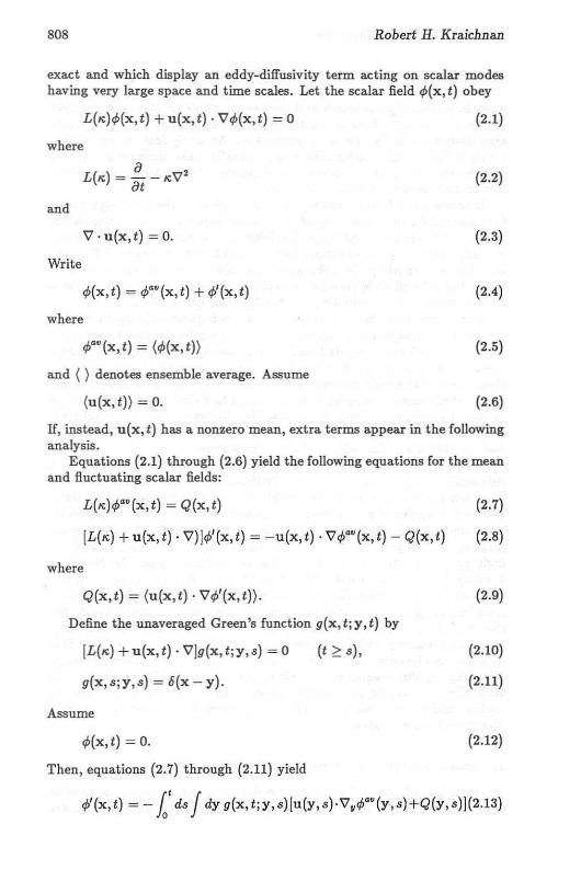
exact and which display an eddy-diffusivity term acting on scalar modeshaving very large space and time scales. Let the scalar field o;6 (x , t) obey

L(,,)0;6(x,t) + u (x , t) . V 0;6(x , t) = 0 (2.1)

where

aL(,,) = - - "v' (2.2)

at

and

V · u(x,t) = O. (2.3)

Write

o;6(x, t) = o;6"(x, t) + 0;6' (x , t) (2.4)

where

o;6· ' (x , t) = (0;6 (x, t» (2.5)

and ( ) denotes ensemb le average. Assume

(u (x , t) = O. (2.6)

If, ins tead, u (x, t) has a non zero mean , extra terms appear in the followinganalys is.

Equations (2.1) through (2.6) yield the following equat ions for the meanand fluctuating sca lar fields:

L( ,,)0;6·' (x ,t) = Q(x,t) (2.7)

IL (,,) + u(x, t) . V)]0;6' (x ,t) = - u (x, t) . V0;6·' (x, t) - Q(x , t) (2.8)

where

Q(x , t) = (u (x , t ) . V0;6' (x,t».

Define the unaveraged Green's function g(x , tj y,t) by

(2.9)

IL(,,) + u (x, t) . VJg(x, t ;y , s) = 0

g(x,s;y,s) = 6(x - y) .

Ass ume

(t ~ s) , (2.10)

(2.11)

(2.12)o;6(x , t) = O.

Then, equat ions (2.7) through (2.11) yield

o;6' (x , t) = - 10' ds I dyg (x, t;y, s)[u (y, s). V,0;6·' (y, s)+Q(y,s)](2.13)

Eddy Viscos it y and Di ffusivity

and, therefore,

Q(x , t) = 8~; 10' dsI dy A; (x,t;y ,s)Q(y,s )

8 l' I 84>"" (y ,s)+ -8 ds dy I';;(x ,t;y, s) 8 .~ 0 W

where equat ion (2.3) is used and

A;(x,t;y,s) = (u;(x ,t )g(x,t;y,s ) ,

I'.;(x ,t;y, s) = (u.(x, t )g(x , t ;y,s)u;(y,s) .

809

(2.14)

(2.15)

(2.16)

No approximation has been made so far. Suppose that 4>Qtl (x,t) hasspace and time scales very long compared to those that are significant inu(x , t). Then, equat ions (2.7) and (2.14) yield an equation of motion for4>Qtl(x, t) in which the coefficient functions are averages whose correlationscales are characteristic of the velocity field. Now let the slowly varying field4>"O(y,s) in (2.14) be expanded in a Taylor series about (x, s). Assume thatthis series has at least a finite radius of convergence in

or that the series is asymptotic in some suitable sense about ei = O. Equa­t ion (2.14) may be exp anded in the form

Q(x, t) = Y (x , t ) + Z(x, t )

where

(2.17)

8 l' 8Q (x ,s)Y (x, t ) = -8 ds[A;(x, t; s)Q(x, t) + A;;(x, t;s ) 8 + .. .],Xi 0 Xi

(2.18)

z\x, t) =

8 (' [ 84>(x ,s) 8'4>"O (X,s) ]-8 . n ds I';;(x ,t ;s ) 8 . + 1'.;m(x ,t; S) 8.8 +... , (2.19)XIJ ~ x, x, xm

and

etc.

A;(x ,t; s) = I dy(u;(x, t )g(x ,t; y,s) ,

A;;(x, t; s) = I dy(u. (x,t)g (x , t;y,s)~;) ,

I';;(x,t ;s) = I dy (u;(x ,t)g(x,t;y, s)u;(y , s» ,

(2.20)

(2.21)

(2.22)

810 Robert H. Kraichnan

l"ijm(X,t; s) = ! dY(Ui(X ,t)g(x ,t;y,s)Uj(y,s)Em}, (2.23)

etc.Equations (2.17) through (2.19) st ill provide a formally exact represen­

tation of Q(x , t) , imp licitly in powers of a ratio f.,. /£., where f.,. and £. arecharacter istic spatial scales of the velocity field and the mean scalar fieldq,'., respectively. An equivalent of (2.22) was first der ived by Corrsin [31.

Q(x,t ) may now be expressed in powers of lu/l~ by an iterat ion so lu­tion of equation (2.17). The leading term in th is expansion is the term inJ.Li;(X,t;s). lfthe s-variat ion of ¢av(x, s) is neglected in comparison to thatof .uij(X, t; s), there results th e equation of motion for q,GlI (X, t) :

L(I< )q,' · (x , t ) = 88 [J<; j(x ,t ) 8q,'.(x,t)]X j aXj

wher e

I<;j(x,t) = fa'l"ij(x ,t;s)ds.

(2.24)

(2.25)

The tensor Ki"(X ,t) is the exact asymptotic ed dy diffusivity in the sensethat (2.24) is asymptotically exact if the spatial and temporal variationof q,'·(x,t) is infinitely slow compared to that of u (x , t ). No closu re ap­proximation has been mad e . It is assumed, via equation (2.12) , that themean scalar field is switched on at t = 0 (or, equivalent ly, that the velocityfield is switched on at t = 0). Statist ical homogeneity or stationarity ofthe velocity field is not assumed, but if the velocity field is statistically ho­mogeneous and isotropic , the exact asymptotic scalar eddy diffusiv ity (inthree dimensions) is

1I<eddy(t) = 3I<ii (X, t ). (2.26)

3 . Lagrangian transformation

There are two principal reasons for transforming the Eulerian formulae ofsection 2 into Lagrangian expressions. First, the results reproduce Taylor's1921 formula [41 for eddy diffus ivity when the molecular diffusivity I< van­ishes, and thereby provide an exact generalization of Taylor's formula to thecase of nonzero K . Second, the Lagrangian expressions are physically moreappropriate because they eliminate confusing (and canceling) convectioneffects in the amplitude factors from which the right -hand sides of (2.20)through (2.23) are constructe d. Thereby, these express ions become moresuitable for statist ical approximation. Th is is discusse d further in sect ion 5.

The Lagrangian transformation of equa t ions (2.18) an d (2.19) (withequations (2.20) through (2.23) inserted), has the effect of changing thespacetime integrals on the right-hand sides into integrals backward in timefrom the present instant t, along a space-filling family of fluid-element tra­jectories. This can be done by introducing the generalized velocity field

E ddy Viscosity and Di/fusivity 811

u (x , t ls ) and scalar field .p(x, tls ) defined as follows: u(x,t ls) is the ve­locity field measured at time s in that fluid element whose trajectorypasses through the spacetime point (x ,t) , with a. corresponding meaningfor .p(x , tis) 15J. The Eulerian fields are then

u.(x ,t) = u;(x,t lt), .p(x , t ) = .p(x, tlt) ,

while the usual Lagrangian velocity field is

ui(x,t) = u.(x , Olt).

(3 .1)

(3.2)

A generalized Green's funct ion may also be defined: g(x, tlsix', t' ls') is theprobability density that scalar concentration found at time s' in the fluidelement whose trajectory passes through (x', t') appears "at time s in thefluid element whose trajectory passes through (x , t) . If I< = 0 (no moleculardiffusivity),

g(x,tls;x',t ls') = S(x - x ') (all s and s'). (3.3)

(3.4)

That is , the scalar concentration in a fluid element is indep end ent of thetime of measurement. Equations of motion for the generalized fields andthe generalized Green's function have been given elsewhere 15].

The transformation to Lagrangian representation is effected by express­ing the integration in equations (2.20) through (2.23) in terms of the newvector variable z(y,t Js), defined in harmony with the preceding definit ionsas the position at time s of the fluid element whose trajectory passes through(y, t ). The transformat ion is volume preserving , in consequence of (1.3) sothat dz = dy. It follows from the definitions of the generalized functionsthat

u[z (y, t ls),sJ == u (y , t [s ), et c .

Then, equations (2.20) through (2.23) may be rewr itten as

),;(x, t; s) = I dy (u;(x , t)g(x, t it; y , t is)), (3.5)

),;;(x,t;s) = I dy (u;(x,t)g(x,t lt ;y, t ls) t ;(y, t ls) ), (3.6)

JL;;(x,t ;s) = I dy(u;(x,t)g(x ,tlt;y,t ls)u;(y,t Js)), (3.7)

I";m(x , t ; s ) = I dy(u;(x , t)g(x , t lt;y, t Js)u;(y , tis) tm(y, t is) ) , (3.8)

where

t ;(y ,t ls) = z;(y,t ls) - X;. (3.9)

If I< = 0, it follows from (3.3) and (2.6) that (3.5) th rough (3.8) reduce to

812

>..(x,t;s) = 0,

>..;(x,t;s) = (u. (x, t )€;(x , t ls)) ,

I'.; (x , t ;s ) = (u. (x , t )u;(x , t ls )),

1";m(X, t ; S) = (u, (x,t)u; (x , tls )€m(X,tIS )) .

Robert H. Kraichnan

(3.10)

(3.11)

(3.12)

(3.13)

(3.15)

Equation (3.12) is equiva lent to Taylor's 1921 formula for eddy diffusiv­ity, the difference being that the Lagrangian velocity in (3.12) is referredto posit ions of fluid elements at time t, while that in Taylor's formula isreferred to positions at the initial instant. The entire expansion of whichequations (3.10) through (3.13) give the leading terms is equivalent to aninfinite-series equation of motion for c/>CUJ (x ,t) of Moffatt's Lagrangian form(6-8). A difference is that the present expansion retains nonlocality in time,while in Moffatt 's form only present values of the mean field appear. Afurther difference is t hat the reversion of power series which underlies Mof­fatt's form is not needed here . Moffat t 's form of expansion gives an elegantexpression of turbulent diffusion of weak magnet ic fields [6-8J. However,serious complications arise if the same kind of expansion is att empted foreddy-viscosity effects . Although the vorticity field obeys the same formalequation of mot ion as the weak magnetic field, the intrinsic statistical de­pendence of velo city on vortici ty plays a crucial role.

It should be noted that the case K. = 0 can be made to include the caseof nonzero K. by the artifice of representing molecular diffusivity as due to avery rapid and small-scale component of the velocity field. Nevertheless, itis of practical inte rest to have the expl icit formulae (3.5) through (3.8) fornonzero It . Moreover, it can be useful to make only a partial transformat ionto Lagrangian coordinates, so as to lump small-scale, rapid modes of theturbulent velocity field with the molecular diffusivity. This can be doneby using a filtered velocity field to define t he Lagrangian transformation.Equations (3.5) through (3.8) ret ain the same forms, but the meani ng ofthe generalized fields is altered. If v (x, t) is th e filt ered field obtainedby passing the Eulerian field u (x , t) through a low-pass wavenumber filteror other appropriate filter, then the generalized fields are related to theEulerian fields by [51 :

[~ + v (x , t) · 'i7]u, (x, t is) = 0, u,(x,sls) = u. (x , s), (3.14)

[: t + v (x, t). 'i7] ¢(x , tls) = 0, ¢ (x,sl s) = ¢ (x ,s).

The vector field z(x,t js) now represents trajectories of particles carried bythe field v(x, t). Only if v(x, t) = u(x, t) and I< vanishes do equations(3.5) through (3.8) reduce to (3.10) through (3.13). In either event, (3.5)through (3.8) remain exact equations.

Eddy Viscosity and Diffusivity 813

4. Exact analysis for eddy viscosity

The Nav ier-Stokes (N-S) equat ion leads to expansions like those deve lopedin sect ions 2 and 3, and associated expressions may he constructed for theasymptotic eddy viscosity acting on slowly varying modes . However, thereare important differences arising from the nonlinearity of the equat ions ofmotion and from the vector character of the velocity field. The nonlinear­ity implies that an asymptotic eddy viscosity, independent of the slow fieldit acts upon , is well-defined only if the slow field has infinitesimal ampli­tude. The vector nature of the field adds qualitatively new features to theexpansions.

Let the N-S equation for an incompressible velocity field u(x, t) in acyclic box or infinite domain he written as

1L(v)u,(x, t) = - z-P;;m('I7 )[U;(x , t)um(x , t)J ,

where L is defined by equation (2.2), v is kinemat ic viscosity,

(4.1)

(4.2)

P,;('I7) = 8,; - '17-''17,'17;,a

'17, '" -a.x, (4.3)

Here, P';m('I7 ) expresses eliminatio n of the pressure field via (2.3). P,;('I7)is a project ion operator which suppresses the longitudin al part of the vecto rfunct ion on which it operates . Let uftl (x,t) be an infinitesimal mean fieldswitched on as a perturbation at time t = O. Assume that the unperturbedfield u; (x, t ) has zero mean for all t , an d let u:(x ,t) be the pertu rbat ioninduced in the fiuctuat ing field. Then , equation (4.1) yields t he followingequat ions for the evolution of u '" and u ':

L(v)ui"(x, t) = Q,(x,t),

Q,(x ,t) = - P';m('I7)(u;(x , t)u:'(x, t)),

[8;mL(v) + P';m('I7)u;(x , t) ]u:'(x, t)= - P';m('I7 )1u; (x , t )u:::, (x , t )l - Q,(x,t).

(4.4)

(4.5)

(4.6)

As in the scalar case, uHx,t) can be expressed as a spacetime integral overa Green's function. The latter is now a solenoidal tensor defined by

[8;mL(v ) + P';m('I7) u;(x ,t)Jgmn(x ,t ;y, s) = 0,

gmn(x,s ;y, s) = Pmn('I7)8(x - y).

(4.7)

(4.8)

814 Robert H. Kraicbnan

If t he integral expression for u:(x, t) is substituted into (4.5), the result maybe written in a form analogous to (2.14) :

Q;(x, t)

where

= V; I.' dsJdY[A;;n(x ,t;y, s)Qn(Y,s)

( ) au~U (y , s) ( ) .U( )]+ J1.ijan x,t;y,s a + ~jn x,t;y,s Un Y ,SY.

(4.9)

A;;n(X, t; Y,S) P;m(V )( [U;(X , t)gmn (X,t; y, S)

+ um(X, t)g;n(X,t; y,s)]) , (4.10)

!';;.n(x, t; y , s] P;m(V)( [u;(x , t )gm.(x, t; y, s)

+ um(x, t )g;.(x, t ;y , s))P..(V.)u.(y, s)}, (4.11)

,,;;.(x, t; y, s ) P;m(V)(lu;(x, t}gm.(x , t; y, s}

+ um(x, t}g;.(x , t; y , s})P••(v.)au.(y , s )a y. }. (4.12)

In these equat ions, Pim(''V,,) operates on fun ctions of y . Bo th the symmetryof P;;m(V) and th e property (2.3) are used in obt aining the right-hand sides.There are some differences from the scalar case. First , J1.ijan(X,t jy, s) andQi;n(X, tj y, s) are opera to rs; Prn C~'u) and Pr60 (''VtI) operate on everything totheir right. Second, the term in !Xi;n has no count erpart in the scalar case .It involves u:U(y,s) itself rather than its spat ial derivative . This term isanalogous to the a-effect term in the equat ion for a weak magnetic fielddiffused by turbulence [61.

As in the scalar case, u(lU(y, s) can be expanded in power series aboutthe point (x,s). Hthe leading Cli;n term is nonzero, it is the leading term inthe entire expansion, and as a consequence, in contrast to the scalar case ,the Aiin term can contribute to the exact asymptot ic eddy viscosity.

The power-series expansions are formally stra ightforward. If the leading(Xiin term vanishes , as it does in reflection-invariant homogeneous turbu­lence , the exact asymptotic form taken by' (4.9) in limit of infinitely slowlyvarying u"''' is

au~U(x , t)Q;(x ,t ) = V; v;;•• (x, t}-'--"ac'---'--!­

x.

where

vii",n(X,t) = itds f dY[~ii",n (x,t;y,s) + (Xiin (x ,t;y,s)€",] .

(4.13)

(4.14)

In equation (4.14) , ~ii",n and Ctiine", reduce to functions; the P operato rs nolonger act on u'" . If the turbulence is statist ically homogeneous, isotropic,and nonhelical , the exact asymptotic equat ion of motion for uat' reduces to

L(v)u ·U(x, t ) = v"",. (t )V'u· · (x, t ), (4.15)

Eddy Viscosity and Di ffusivity

with

815

(4.16)

in three dimensions.It should be noted that when Vi;an (X, t) for homogeneou s turbulence is

transformed into the wavevector domain, the eo factor in (4.14) becomes aderivat ive with respect to wavevector. Such derivatives do not appear inthe wavevector representation of the asymptotic eddy diffusivity.

The Lagrangian transformation of the eddy viscosity can be carriedout as in the scalar case, but care must be taken to correct ly handle thederivatives with respect to Yj derivatives with respect to z (y, tis) are notequivalent to derivatives wit h respect to y. IT the Eulerian fields

W,~ (y,s) = PmCI7.)u.(y,s),

[au.(y,s)]

Xm.(Y,s) = p,.('V.) €. aYn

(4.17)

(4.18)

are delined, the generalized lields wm.(y,tls) and Xm.(y,tls) may be de­lined by an equation like (3.14) . Then, (4.14) can be transformed to

Vij.n(X,t) = Pim ('V)1.'JdY([Uj(x, t)gm,(x,t lt;y,tls)

+ um(x, t)gj,(x, t it;y , tls)J [wm,(y, t is)+ X,n. (y,tls)]) . (4.19)

The equations of mot ion for gm...[x, tjt;y , tis ) have been described elsewhere­[5]. If the power-series expans ion of u °t/(y , s) of (x,s) is carried to higherterms, the Lagrangian transformation can be carried out term by term inthe entire resulting series for Qi(X,t) .

5. Breaking t he averages

The expressions for asymptotic eddy diffusivity and eddy viscosity derivedin sections 2 through 4 are exact under the assumptions made . However,they involve rather complicated statistical averages. It is tempting to tryto approximate the expressions by factoring them into products of simpleraverages . Most of the closure approximations that have been proposedfor eddy diffusivit y and eddy viscosity involve such facto ring, performedaccording to a variety of rationales.

Consider the approximation to the eddy diffusivity obtained by factoringthe Eu lerian express ion (2.22) and insert ing the result int o (2.25):

ltij(X,t) = 1.' dsI dY[(Ui(X, t)Uj(y, s)}(g(x, t;y, s))]. (5.1)

816 Robert H. Kraichnan

What can be said about the validity of this approximation? First it maybe noted that (5.1) alternatively can be obtained as a consequence of thedirec t-interac t ion app rox imatio n (DIA) for the turb ulent diffusion of a pas­s ive scalar [9], and it has bee n prop osed independently in the form of anatural approximat ion for the Lagrangian velocity covariance [3,10]. TheDIA also yields equations which determine the evolut ion of the covarianceand mean Green's function that appear in (5.1) . Numerical integrations in­dicate that both (5.1) an d the DIA values are good qualit ative and quant ita­tive approximations in isotropic turbulence, provided that the wavenumberspectrum of the Eulerian velocity field is concentrated about its center ofgravity [11] .

If instead the spectrum is diffuse in wavenumber, (5.1) introduces quali­tative errors because of convect ion effects. (This is independent of whetherthe DIA is used to evaluate the right side.) To see this, suppose that theEulerian velocity spectrum consists of a strong low-wavenumber part and ahigh-wavenumber part, the two widely separated in wavenumber. Convec­tion of the high-wavenumber field by the low-wavenumber field will inducerapid decorrelation of the latte r in time, and this makes both averages onthe right side fall off rapidly. However, the product average, in the originalexact expression (2.22), does not show this effect because the convectioneffects in the three factors are correlated.

The spurious convection effects in (5.1) do not arise if the Lagrangianaverage (3.7) is factored to give the approximat ion

l"i; (X,t;S) = ! dy[(u; (x,t )u;(y, tls ))(g(x,tlt,y, tls )) ]. (5.2)

(5.3)

In the case /'C = 0, the g funct ion is statist ically sharp with the value (3.3),and (5.2) is identical with t he exact express ion (3.12). If Ie is nonzero,g(x , t lt ;y,t ls) fluct uates because of distortion of fluid elements by the flow.The distortion makes the scalar gradient in a given fluid element fluctuateand hence makes the molecular diffusion fluctuate. However, it is plausi­ble that this fluctuat ion is much more weakly correlated with fluctuationsin u; (x , t Is) t ha n the convect ion effects which afflict th e factoring of theEulerian expression (2.22). Thus, it is plausible t hat (5.2) remains a goodqualitative and quantitat ive approximat ion even for nonzero /'C .

A more drastic approximation is to simply replace the g function in(3.7) by t he value it would have in the absence of the turbulence:

O( I . I ) -[ ( )]- 3/' ( - Ix - y l')9 x ,t t, y, ts -4"I<t-s exp [41« t - s )] .

This ap proximation ignores complete ly the effects of straining of fluid ele­ments on molecular diffusion. Itshould, nevertheless, have a greater domainof validity than the Eulerian factoring (5.1).

Approximations to the exact asymptot ic eddy viscosi ty also may beconstructed by factoring the Eulerian and Lagrangian expressions. As inthe scalar case, the Eulerian factoring introduces spurious convection effects

Eddy Viscosity and Dilfusivity S17

when the velocity spectrum encompasses a wide range of wavenumbers.These effects do not ar ise in the factoring of (4.19), which leads to theapproximation

V';.n(x,t ) = P'm('i7) fo' Jdy[W;,..(x,t;y,t ls)Gm.(x,t lt;y,tls)

+ Wm,..(x,t;y,tls)G;.(x,t;y,t ls)j. (5.4)

Here,

W;...(x , t; y, ti s) = (u; (x, t )[w...(y , tis) + X...(y , tis)]) (5.5)

conta ins the Lagrangian velocity covariance, mod ified by the solenoidalprojection operator, while

(5.6)

is the mean Lagrangian Green's tensor.In contrast to the scalar case, the inviscid Lagrangian Green's tensor

is not simply the solenoidal projection of a a-functionj it exhibits effectsof st raining and pressure fluctuations. Consequently, replacing Gmr by itspurely viscous va lue may not to be a vali d further approximation in high­Reynolds-number turbulence. Perhaps more just ified is the approximationof W j r na by a simpler Lagrangian tensor:

W;... (x,t;y,t) = P,.('i7,)U;.(x,t;y,tls)ou.(y, t is)+ p••('i7,)(u;(x ,t)€.(y,tls) 0 ) (5.7)

Yn

where

U;.(x,t;y,tJs) = (u;(x,t)u.(y,tJs) ) (5.S)

is the Lagrangian velocity covariance.Equations (5.2), (5.4), and (5.7) alternatively are obtained as conse­

quences of the Lagrangian-history DIA [5J, which provides approxima­tions for the Lagrangian functions G, Uja, and G mr in terms of Eulerianquantities . It would be interesting to see how good an approx imation(5.2) and (5.4) provide (with or wit hout equa tion (5.7)) if exac t valuesof G, Gmn Wjm1u and U;o. are used.

The exact formulas of sect ion 4 assume that the large-scale mean fieldhas infinitesima l amplitude, but in typical applications, the modes of largespatial scale have most of the kinetic energy. It is therefore important todiscuss the errors associated with finite mean-field excitation, both for theexact asymptotic formulas and for the approximate factorings presented inthe present sectio n. Modes of large spatial scale exert two (interacting)kinds of effect on modes of small spatial scale: convection and distortion.The former is proportional to the large-scale velocity and the latter to thelarge-scale rate-of-strain tensor. If the turbulence is statistically homo­geneous, convection effects do not alter the energy transfer between the

818 Robert H. Kraichnan

mean field and the small-scale turbulence and therefore do not alter theeddy viscosity. This is expressed formally by the invariance of the ex actasymptot ic exp ress ions (4.10) through (4.12), (4.14), (4.16), and (4.19) toGalilean transformations. The exact eddy-diffusiv ity expressions (2.2 2),(2.25), and (3.12) also ar e invar iant under Gal ilean transformation whenthere is statistical homogeneity. Distortion by the large-scale mean fie lddoes affect the energy transfer. Thus, the effect ive eddy viscosity exertedon a finite-strength large-scale field differs from the asymptotic value if therates of strain associated with the large-scale field are comparable to thoseintrinsically associated with the small-scale turbulence.

Galilean invariance extends also to the factoring approximat ions (5.1),(5.2), and (5.4). In the case of the Euler ian factoring (5.1) and its coun­terpart for eddy viscosity, both the covariance and Green's function factorson the right-hand side change under a st atistically sharp Galilean trans­formation, but the changes exac tly compensate when there is statisticalhomogeneity.

The convection effects of large-scale Buctuating fields are associatedwith behavior under random Galilean transformation: the addition to thetotal velocity field of an x-independent velocity which is randomly differentin each real izat ion 151 . Both the Eulerian and Lagrangian exact asymp­totic eddy-d iffusivity and eddy-viscosity formulas are invariant under ran­dom Galilean transformation, but the factored approximations behave dif­ferently. The Lagrangian factorings (5.2) an d (5.4) are invariant becauseboth covariance and Green's function factors are invariant. However, thesefactors both change under transformation in the Eulerian case (5.1) andthe corresponding factoring for eddy-viscosity. Because of the breaking ofthe averages, the changes do not compensate, as they did for statist icallysharp transformation, and the resulting eddy diffusivity and eddy viscosityshow spurious change under the transformation (see the discussion follow­ing equa t ion (5.1)).

Eddy viscosity traditionally is positi ve, corresponding to energy flowfrom the large-scale field to the small-scale turbulence. However, variousnegative-viscosity phenomena, in which the direction of energy flow is re­versed, have been described 112-201. It should be noted here that the nega­tive viscosity effect in two-dimensional turbulence [12-15], which can occurwith isotropic statistics, and the corresponding effect in three dimensions115-201 , which depends essentially on anisotropy of the small-scale statis­tics , are both contained in the exact asymptotic eddy expression (4.14).Moreover, they survive in the factor ing approximation (5.4) and under thefurther approximation of using Lagrangian-history DIA to evaluate the co­variance and Green's funct ion.

The recently descrihed "an isotropic kinetic alpha (AKA) effect" 1201is a reverse-energy-flow phenomenon that involves the «tin term in (4.9) .There are several interesting features. First, the AKA effect results ingrowth of large-scale helical waves of a particular sign, and therefore, thesmall-scale field defines a screw sense . Nevertheless, the small-sca le field

Eddy Viscosi ty and Dilfusivity 819

has no helicity. Second, the maintenance of the AKA effect in steady staterequires that non-Galilean-invariant , small-scale, zero-mean forcing termsbe added to the Navier-Stokes equation. In the presence of such forcing, anadditional term appears in (4.9) which involves the functi onal derivative ofthe Green's tensor with respect to the mean velocity field.

Acknowledgments

It is a pleasure to acknowledge conversations with U. Frisch and V. Yakhotwhich contributed to this paper. B. Nicolaenko has kindly reported errorsin the manuscript. This work was supported by the Nat ional Science Foun­dation under Grant AT M-8508386 to Robert H. Kraicbnan, Inc., and by theDepartment of Energy under Contrac t W-7405-Eng-36 with t he Un iversityof California, Los Alamos National Laboratory.

R eferences

II ] H. A. Rose, J ournal of Fluid Mechanics, 81 (1977) 719.

[2] J. Smagorinsky, Mon. Wea. Rev., 91 (1963) 99.

[3J S. Corrsin, in Proceedings of the Oxford Symp osium on Atmosp heric Diffu ­sion and Air Pollution (Academic Press, New York, 1960) 162.

[4] G. 1. Taylor, Proc. London Math . Society, 20 (1921) 196.

15] R. H. Kraichnan, Physics of Fluids, 8 (1965) 575.

[6] H. K. Moffatt, Journal of Fluid Mechanics, 65 (i974) 1.

17] R. H. Kraichnan , Journal of Fluid Mechanics, 75 (1976) 657.

[8J R. H. Kraichnan, Phys. Re v. Letters, 42 (1979) 1677.

[9J P. H. Roberts, J ournal of Fluid Mechanics, 11 (1961) 257.

[10] P. G. Saffman, Appl. Sci. Res. A, 11 (1962) 245.

[11] R. H. Kraichnan , Physics of Fluids, 13 (1970) 22.

[12] R. Fjoroft , Tellus, 5 (1953) 225.

[13] R. H. Kraichnan , Physics of Fluids, 10 (1967) 1417.

[14] R. H. Kraichnan, J. Atmos. Sci., 33 (1976) 1521.

[15] V. St arr, Physics of Negative Viscosity . (McGraw-Hill, New York, 1968) .

[16] G. Sivashin sky, Physica D, 17 (1985) 243.

117] G. Sivashinsky and V. Yakhot, Physics of Fluids, 28 (1985) 1040.

[18] B. J . Bayly and V. Yakhot, Phys. Rev. A , 34 (1986) 381.

820 Robert H. Kraichnan

[19J V. Yakhot and G. Sivashinsky, Phys. Rev. A , 3S (1987) 815.

1201 U. Frisch, Z. S. She, and P. L. Sulern, Physica D, submitted.