ECS 452: Digital Communication Systems 2013/1

HW 1 — Due: July 24

Lecturer: Prapun Suksompong, Ph.D.

Instructions

(a) ONE part of a question will be graded (5 pt). Of course, you do not know which partwill be selected; so you should work on all of them.

(b) It is important that you try to solve all problems. (5 pt)

(c) Late submission will be heavily penalized.

(d) Write down all the steps that you have done to obtain your answers. You may not getfull credit even when your answer is correct without showing how you get your answer.

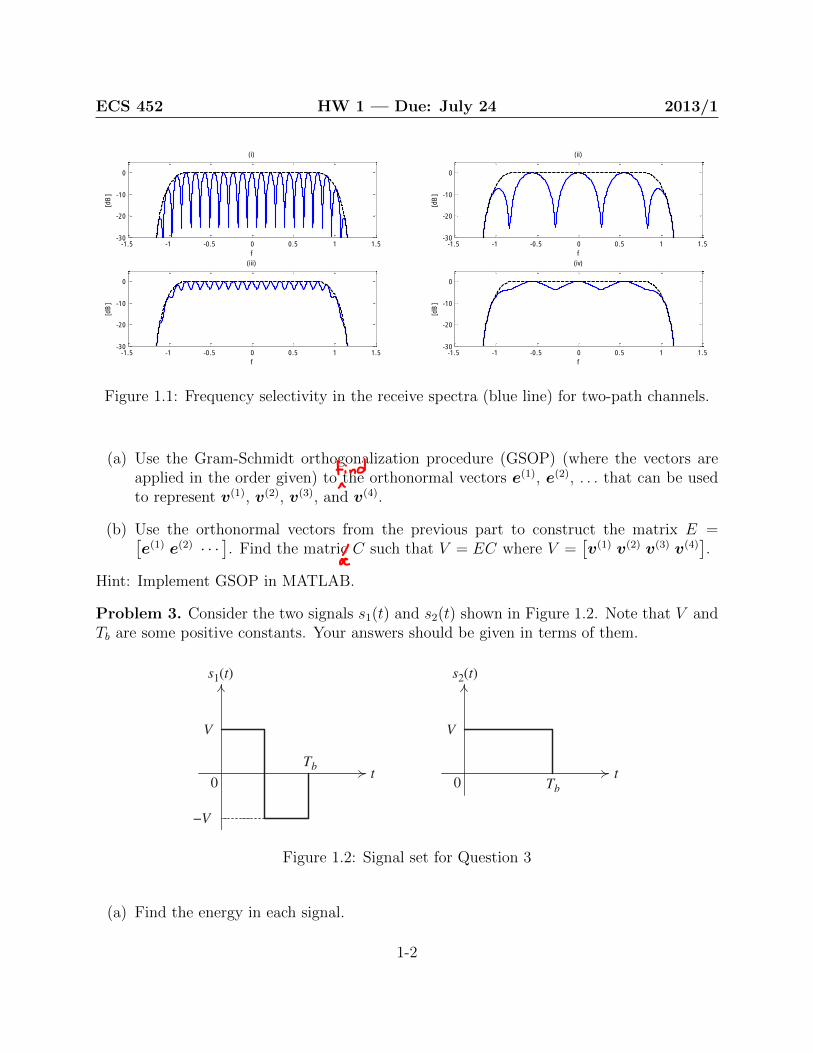
Problem 1. Consider the two-path channels in which the receive signal is given by

y(t) = β1x(t−∆t1) + β2x(t−∆t2).

Four different cases are considered.

(a) Small |∆t1 −∆t2| and |β1| � |β2|

(b) Large |∆t1 −∆t2| and |β1| � |β2|

(c) Small |∆t1 −∆t2| and |β1| ≈ |β2|

(d) Large |∆t1 −∆t2| and |β1| ≈ |β2|

Figure 1.1 shows four plots of normalized1 |X(f)| (dotted black line) and normalized|Y (f)| (blue line) in [dB]. Match the four graphs (i-iv) to the four cases (a-d).

Problem 2. Consider four vectors

v(1) =

1 + j1− j

0

,v(2) =

1−10

,v(3) =

11−1

, and v(4) =

−1−1−j

.

1The function is normalized so that the maximum point is 1 dB.

1-1

ECS 452 HW 1 — Due: July 24 2013/1

-1.5 -1 -0.5 0 0.5 1 1.5-30

-20

-10

0

f

[dB

]

(i)

-1.5 -1 -0.5 0 0.5 1 1.5-30

-20

-10

0

f

[dB

]

(ii)

-1.5 -1 -0.5 0 0.5 1 1.5-30

-20

-10

0

f

[dB

]

(iii)

-1.5 -1 -0.5 0 0.5 1 1.5-30

-20

-10

0

f

[dB

]

(iv)

Figure 1.1: Frequency selectivity in the receive spectra (blue line) for two-path channels.

(a) Use the Gram-Schmidt orthogonalization procedure (GSOP) (where the vectors areapplied in the order given) to the orthonormal vectors e(1), e(2), . . . that can be usedto represent v(1), v(2), v(3), and v(4).

(b) Use the orthonormal vectors from the previous part to construct the matrix E =[e(1) e(2) · · ·

]. Find the matric C such that V = EC where V =

[v(1) v(2) v(3) v(4)

].

Hint: Implement GSOP in MATLAB.

Problem 3. Consider the two signals s1(t) and s2(t) shown in Figure 1.2. Note that V andTb are some positive constants. Your answers should be given in terms of them.

178 Optimum receiver for binary data transmission�

−V

t

V

0

Tb

t

Tb1

0

Tb

t

V

0 Tb

Tb−1

t0 Tb

Tb1

(a)

(b)

φ1(t) φ2(t)

s2(t)s1(t)

�Fig. 5.5 (a) Signal set for Example 5.2, (b) orthonormal functions.

0

E

E

φ2(t)

φ1(t)

s2(t)

s1(t)�Fig. 5.6 Signal space representation for Example 5.2.

Graphically, the orthonormal basis functions φ1(t) and φ2(t) look as in Figure 5.5(b) andthe signal space is plotted in Figure 5.6. The distance between the two signals can be easilycomputed as follows:

d21 =√

E + E = √2E = √2√

E. (5.35)

�

In comparing Examples 5.1 and 5.2 we observe that the energy per bit at the transmitteror sending end is the same in each example. The signals in Example 5.2, however, are closertogether and therefore at the receiving end, in the presence of noise, we would expect moredifficulty in distinguishing which signal was sent. We shall see presently that this is thecase and quantitatively express this increased difficulty.

Example 5.3 This is a generalization of Examples 5.1 and 5.2. It is included princi-pally to illustrate the geometrical representation of two signals. The signal set is shown

Figure 1.2: Signal set for Question 3

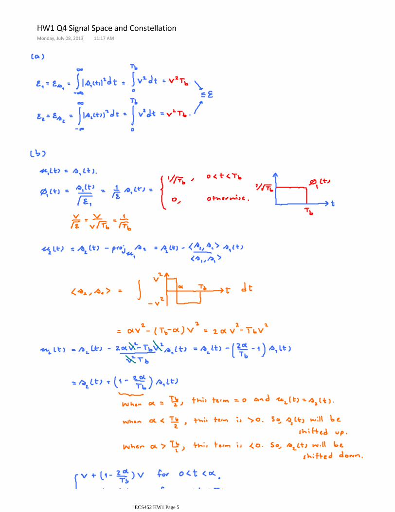
(a) Find the energy in each signal.

1-2

ECS 452 HW 1 — Due: July 24 2013/1

(b) Use the Gram-Schmidt orthogonalization procedure (GSOP) (where the signals areapplied in the order given) to find two orthonormal functions φ1(t) and φ2(t) that canbe used to represent s1(t) and s2(t).

(c) Find the two vectors that represent the two waveforms s1(t) and s2(t) in the new(signal) space based on the orthonormal basis found in the previous part. Draw thecorresponding constellation.

Problem 4. Consider the two signals s1(t) and s2(t) shown in Figure 1.3. Note that V , αand Tb are some positive constants.

179 5.1 Geometric representation of signals s1(t) and s2(t)�in Figure 5.7, where each signal has energy equal to E = V2Tb. The first basis function isφ1(t) = s1(t)/

√E. The correlation coefficient ρ depends on parameter α and is given by

ρ = 1

E

∫ Tb

0s2(t)s1(t)dt = 1

V2Tb

[V2α − V2(Tb − α)

]= 2α

Tb− 1. (5.36)

As a check, for α = 0, ρ = −1 and for α = 12 Tb, ρ = 0, as expected. The second basis

function is

φ2(t) = 1√E(1− ρ2)

[s2(t)− ρs1(t)]. (5.37)

To obtain the geometrical picture, consider the case when α = 14 Tb. For this value of α

one has ρ = − 12 . As before φ1(t) = s1(t)/

√E, whereas the second orthonormal function

is given by

φ2(t) = 2√3V√

Tb

[s2(t)+ 1

2s1(t)

]. (5.38)

The two orthonormal basis functions are plotted in Figure 5.8. The geometrical representa-tion of s1(t) and s2(t) is given in Figure 5.9. Note that the coefficients for the representation

of s2(t) are s21 = − 12

√E and s22 =

√3

2

√E. Since s2

21 + s222 = E, the signal s2(t) is at a dis-

tance of√

E from the origin. In general as α varies from 0 to Tb, the function φ2(t) changes.However, for each specific φ2(t) the signal s2(t) is always at distance

√E from the origin.

The locus of s2(t) is also plotted in Figure 5.9. Note that as α increases, ρ increases andthe distance between the two signals decreases. �

t0

−V

t

V

0

V

Tb

Tb

s2(t)s1(t)

α�Fig. 5.7 Signal set for Example 5.3.

t

Tb

Tb Tb

Tb

1

0t

3Tb3

04

1

3Tb1−

φ1(t) φ2(t)

�Fig. 5.8 Orthonormal functions for Example 5.3.

Figure 1.3: Signal set for Question 4

(a) Find the energy in each signal.

(b) Use the Gram-Schmidt orthogonalization procedure (GSOP) (where the signals areapplied in the order given) to find two orthonormal functions φ1(t) and φ2(t) that canbe used to represent s1(t) and s2(t).

(c) Plot φ1(t) and φ2(t) when α = Tb

4.

(d) Find the two vectors s(1) and s(2) that represent the two waveforms s1(t) and s2(t) inthe new (signal) space based on the orthonormal basis found in the previous part.

(e) Draw the corresponding constellation when α = Tb

4.

(f) Draw s(2) when α = k10Tb where k = 1, 2, . . . , 9.

1-3

HW1 Q1 Two-Path ChannelsMonday, July 08, 2013 1:53 PM

ECS452 HW1 Page 1

HW1 Q2 GSOP for Complex-Valued VectorsMonday, July 08, 2013 1:48 PM

ECS452 HW1 Page 2

ECS452 HW1 Page 3

HW1 Q3 Signal Space and ConstellationMonday, July 08, 2013 10:39 AM

ECS452 HW1 Page 4

HW1 Q4 Signal Space and ConstellationMonday, July 08, 2013 11:17 AM

ECS452 HW1 Page 5

ECS452 HW1 Page 6

ECS452 HW1 Page 7

ECS 452: Digital Communication Systems 2013/1

HW 2 — Due: Not Due

Lecturer: Prapun Suksompong, Ph.D.

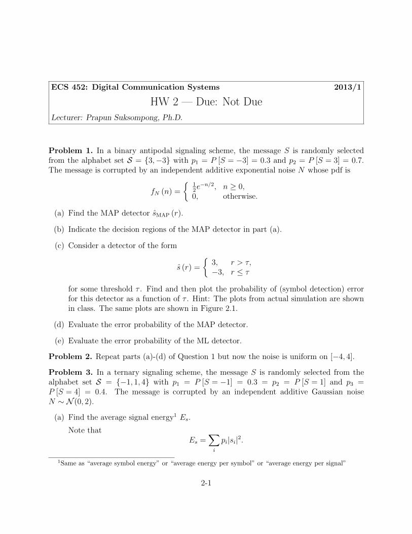
Problem 1. In a binary antipodal signaling scheme, the message S is randomly selectedfrom the alphabet set S = {3,−3} with p1 = P [S = −3] = 0.3 and p2 = P [S = 3] = 0.7.The message is corrupted by an independent additive exponential noise N whose pdf is

fN (n) =

{12e−n/2, n ≥ 0,

0, otherwise.

(a) Find the MAP detector sMAP (r).

(b) Indicate the decision regions of the MAP detector in part (a).

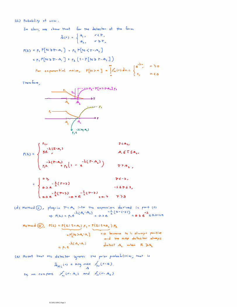
(c) Consider a detector of the form

s (r) =

{3, r > τ,−3, r ≤ τ

for some threshold τ . Find and then plot the probability of (symbol detection) errorfor this detector as a function of τ . Hint: The plots from actual simulation are shownin class. The same plots are shown in Figure 2.1.

(d) Evaluate the error probability of the MAP detector.

(e) Evaluate the error probability of the ML detector.

Problem 2. Repeat parts (a)-(d) of Question 1 but now the noise is uniform on [−4, 4].

Problem 3. In a ternary signaling scheme, the message S is randomly selected from thealphabet set S = {−1, 1, 4} with p1 = P [S = −1] = 0.3 = p2 = P [S = 1] and p3 =P [S = 4] = 0.4. The message is corrupted by an independent additive Gaussian noiseN ∼ N (0, 2).

(a) Find the average signal energy1 Es.

Note thatEs =

∑i

pi|si|2.

1Same as “average symbol energy” or “average energy per symbol” or “average energy per signal”

2-1

ECS 452 HW 2 — Due: Not Due 2013/1

8

-10 -8 -6 -4 -2 0 2 4 6 8 100

0.1

0.2

0.3

0.4

0.5

0.6

0.7

P(E

)

Figure 2.1: P (E) for Exponential Noise in Question 1

(b) Find the MAP detector sMAP (r).

(c) Indicate the decision regions of the MAP detector in part (b).

(d) Evaluate the error probability of the MAP detector.

Problem 4. In a ternary signaling scheme, the message S is randomly selected from thealphabet set S = {−1, 1, 4} with p1 = P [S = −1] = 0.41, p2 = P [S = 1] = 0.08 andp3 = P [S = 4] = 0.51. The message is corrupted by an independent additive Gaussian noiseN ∼ N (0, 2).

(a) Find the average signal energy Es.

(b) If the MAP detector is used, find P (E|S = 1); that is, find the probability of (decoding)error given that S = 1 was transmitted.

Problem 5. In a standard quaternary signaling scheme, the message S is equiprobablyselected from the alphabet set S =

{−3d

2,−d

2, d2, 3d

2

}. The message is corrupted by an

independent additive exponential noise N whose pdf is

fN (n) =

{λe−λ, n ≥ 0,0, otherwise.

(a) Find the average symbol energy.

2-2

ECS 452 HW 2 — Due: Not Due 2013/1

(b) Find the average energy per bit.

(c) Find the MAP detector sMAP (r).

(d) Evaluate the error probability of the MAP detector.

(e) Let λ = 1σ. (This is to set VarN = σ2 as in the case for Gaussian noise.) Plot Eb

σ2 vs.

probability of error P (E). Consider Eb

σ2 from -30 to 10 dB.

2-3

HW2 Q1: 1-D MAP Detector and Exponential NoiseMonday, July 15, 2013 10:58 AM

ECS452 HW2 Page 1

ECS452 HW2 Page 2

ECS452 HW2 Page 3

HW2 Q2: 1-D MAP Detector and Uniform NoiseMonday, July 15, 2013 1:33 PM

ECS452 HW2 Page 4

ECS452 HW2 Page 5

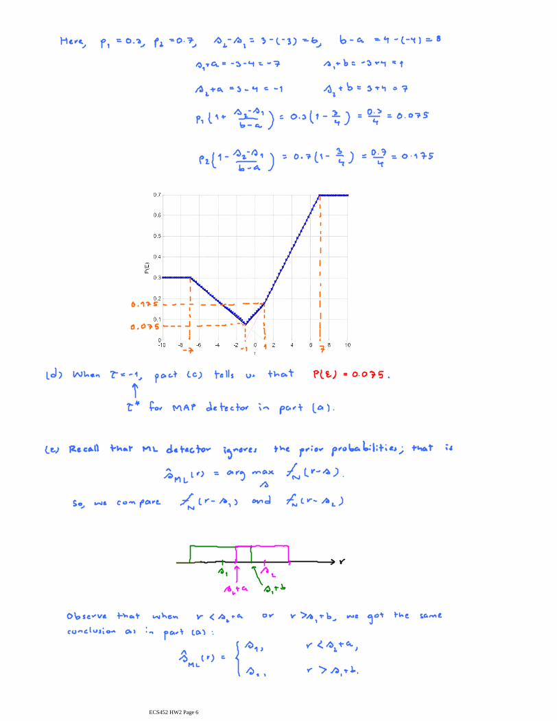
ECS452 HW2 Page 6

ECS452 HW2 Page 7

HW2 Q3: 1-D Multi-Level MAP Detector and Gaussian NoiseWednesday, July 24, 2013 2:31 PM

ECS452 HW2 Page 8

ECS452 HW2 Page 9

HW2 Q4: 1-D Multi-Level MAP Detector and Gaussian NoiseWednesday, July 24, 2013 3:13 PM

ECS452 HW2 Page 10

HW2 Q5: 1-D Standard Multi-Level MAP Detector and Expo NoiseWednesday, July 24, 2013 3:35 PM

ECS452 HW2 Page 11

ECS452 HW2 Page 12