economists’ view of behavior
TRANSCRIPT

Economists’ View of Behavior
C H A P T E R 2C H A P T E R O U T L I N E
Economic Behavior: An OverviewEconomic ChoiceMarginal AnalysisOpportunity CostsCreativity of Individuals
Graphical ToolsIndividual ObjectivesIndifference CurvesOpportunities and ConstraintsIndividual ChoiceChanges in Choice
Motivating Honesty at Merrill LynchManagerial ImplicationsAlternative Models of Behavior
Only-Money-Matters ModelHappy-Is-Productive ModelGood-Citizen ModelProduct-of-the-Environment Model
Which Model Should Managers Use?Decision Making under Uncertainty
Risk AversionCertainty Equivalent and Risk PremiumRisk Aversion and Compensation
SummaryAppendix: Consumer Choice
In May 2002, Merrill Lynch agreed to pay $100 million to settle charges that itsanalysts had recommended stocks to clients that they privately thought were poorinvestments. Internal e-mails provided strong support for this claim leveled by theNew York State attorney general. For example, InfoSpace, an Internet services
company, was rated highly by analysts, yet privately the analysts suggested that it was a“powder keg” and a “piece of junk.” Although InfoSpace’s share price dropped from$261 to $14, Merrill analysts never recommended selling the stock. Merrill analysts
bri75829_ch02.qxd 8/13/08 7:04 PM Page 16

Chapter 2 Economists’ View of Behavior 17
rated Excite@Home “accumulate or buy,” while privately the investment team called ita “piece of crap.”
This episode at Merrill sent shock waves through other major investment houses—indeed through the entire investment community. Other investment firms publiclystated that they were taking strong steps to make sure that the situation at Merrill wouldnot be repeated within their organizations. Fortune magazine ran a cover story entitled,“In Search of the Last Honest Analyst.”1 The scandal generated significant concernsthroughout the world among both the general public and government regulators. Forexample, the New York attorney general began a sweeping investigation of analysts atSalomon Smith Barney and other investment firms that had recommended WorldComto investors. In July 2002, WorldCom became the biggest company ever to file for bank-ruptcy in U.S. history. In December 2002, the nation’s 10 top investment banks agreedto a $1.2 billion settlement with regulators aimed at “protecting investors from broker-ages’ conflicts of interest.”
Managers at Merrill, Salomon Smith Barney, and other investment companies had toact quickly to address this potential problem. As a first step, management had to under-stand what motivated the Merrill analysts to mislead their investment clients. Only thencould they choose a policy to redress the situation. If management thought this problemwas caused by a few dishonest employees, the appropriate response would have been to tryto identify and fire those employees. If, instead, management believed the problem wascaused by disgruntled employees taking out their frustrations on customers, a potentialresponse would have been to adopt a job-enrichment program to increase employee satis-faction and, it would be hoped, analyst honesty. Alternatively, Merrill Lynch might havecreated incentives through its compensation plan that caused its analysts to issue mislead-ing investment reports. If so, the appropriate response would be to restructure its com-pensation plan. Many other assumptions and responses are possible.
The example of Merrill Lynch illustrates a general point: Managers’ responses toproblems are likely to depend on their understanding of people’s motives and their fore-cast of people’s reactions—their responses thus depend on their underlying model ofbehavior. Most managerial actions attempt to change the behavior of individuals, such asemployees, customers, union officials, or subcontractors. Managers with different un-derstandings (or models) of what motivates behavior are likely to make different deci-sions and take different actions.
We begin this chapter by briefly summarizing the general framework economists useto examine individual behavior. Selected graphical tools are introduced to aid our analy-sis. Next, we use this economic framework to analyze the problem at Merrill Lynch.The managerial implications of this analysis are discussed. We contrast this economicview of behavior with alternative views and explore why the economic framework isparticularly useful in managerial decision making. Finally, we analyze decision makingunder uncertainty.
Economic Behavior: An OverviewIndividuals have unlimited wants. People generally want greater wealth, more attentiveservice, larger houses, more luxurious cars, and additional personal material items.They want more time for leisure activities. Most also want to improve the plight ofothers—starving children, the homeless, and disaster victims. People are concernedabout vitality, religion, integrity, and gaining the respect and affection of others.
1June 10, 2002, issue.
bri75829_ch02.qxd 8/13/08 7:04 PM Page 17

18 Part 1 Basic Concepts
In contrast to wants, resources are limited. Households face limited incomes that pre-clude all the purchases and expenditures that household members might like to make.The available amount of land, trees, and other natural resources is finite. There are only24 hours in the day. People become ill; death is inevitable.
Economic Choice
Economic analysis is based on the notion that individuals assign priorities to their wantsand choose their most preferred options from among the available alternatives. If KathyMeaser is confronted with a choice between a laptop or a desktop computer, she can tellyou whether she prefers one over the other or whether she is indifferent between thetwo. Depending on the relative prices of the two products, she purchases her preferredalternative. If Kathy has a weekly budget of $1,000, she considers the many ways shemight spend the money and then chooses the package of goods and services that willmaximize her personal happiness. She cannot make all desired purchases on her limitedbudget. However, this choice is optimal for Kathy, given her limited resources.
Economists do not assert that people are selfish in the sense that they care only abouttheir own personal consumption. Within the economic paradigm, people also care aboutsuch things as charity, family, religion, and society. For instance, Kathy will donate $100to her church, as long as the donation provides greater satisfaction than alternative usesof the money.
Neither do economists contend that individuals are supercomputers that make infal-lible decisions. Individuals are not endowed with perfect knowledge and foresight, noris additional information costless to acquire and process.2 For example, Kathy mightorder an item from a restaurant menu only to find that she dislikes what she is served.Within this economic paradigm, she simply does the best she can in the face of herimperfect knowledge. But she learns from her experience and does not repeat the samemistakes in judgment time after time.3
Marginal Analysis
Marginal costs and benefits are the incremental costs and benefits that are associated withmaking a decision.4 It is the marginal costs and benefits that are important in economicdecision making. An action should be taken whenever the marginal benefits of that actionexceed its marginal costs. Mary O’Dwyer has a contract to help sell products for an office
2Economists sometimes use the idea of bounded rationality. Under this concept, individuals act in a purposeful andintendedly rational manner. However, they have cognitive limitations in storing, processing, and communicatinginformation. It is these limitations which make the question of how to organize economic activity particularlyinteresting. H. Simon (1957), Models of Man ( John Wiley & Sons: New York).
3At least this learning appears to occur outside the comics. For decades, Charlie Brown from Peanuts continued totry to kick the football held by Lucy van Pelt. Yet Lucy always pulled the ball at the last second. Few individualsare as incurably optimistic as Charlie Brown—they learn.
4Technical note: Marginal costs and benefits are typically defined as changes in costs and benefits associated withvery small changes in a decision variable. For instance, the marginal costs of production are the additional costsfrom producing a small additional amount of the product (for instance, one more unit). Often decisions involvediscrete choices, such as whether or not to build a new plant. In these cases, it is not possible to define a smallchange in the decision variable. Incremental costs and benefits are those costs and benefits which vary with sucha decision. For our present discussion, the technical distinction between marginal and incremental is notimportant.
bri75829_ch02.qxd 8/13/08 7:04 PM Page 18

Chapter 2 Economists’ View of Behavior 19
supply company. She is paid $50 for every sales call that she makes to customers. Thus,Mary’s marginal benefit for making each additional sales call is $50. Mary enjoys playingtennis more than selling. If she places a marginal value of more than $50 on the tennis thatshe would forgo by making an extra call, she should not make any more sales calls thatday—the marginal costs would have exceeded the marginal benefits. She continues tomake additional sales calls as long as the reduction in tennis playing is valued at lessthan $50.5
Marginal analysis is a cornerstone of modern economic analysis. In economic deci-sion making, “bygones are forever bygones.” Costs and benefits that have already beenincurred are sunk (assuming they are nonrecoverable) and hence are irrelevant to thecurrent economic decision. Mary paid $5,000 to join a tennis club last month. This feedoes not affect her current decision of whether to play tennis or make an extra sales call.That expenditure is ancient history and does not affect Mary’s current trade-offs.
As another example, consider Ludger Hellweg who owns a company that installs woodfloors. He is offered $20,000 to install a new floor. The cost of his labor and other oper-ating expenses (excluding the wood) are $15,000. He has wood for the job in inventory.It originally cost him $2,000. Price increases have raised the market value of the woodto $6,000, and this value is not expected to change in the near future. Should he acceptthe contract?
He should compare the marginal costs and benefits from the project. The marginalbenefit is $20,000. The marginal cost is $21,000—$15,000 for the labor and operatingexpenses and $6,000 for the wood. The historic cost for the wood of $2,000 is notrelevant to the decision. To replace the wood used on this job costs $6,000. Since themarginal costs exceed the marginal benefits, Ludger would be better off rejecting thecontract than accepting it. This example illustrates that in calculating marginal costs, itis important to use the opportunity cost of the incremental resources, not their historic(accounting) cost.
MANAGERIAL APPLICATIONS
Marginal Analysis of Customer ProfitabilityFirst Union Corp. (since acquired by Wachovia) used a computer program it called Einstein to rank customers based ontheir profitability. “Profitable” customers keep several thousand dollars in their accounts, use tellers less than once a month,and rarely make calls to the bank’s customer call center. “Unprofitable” customers make frequent branch visits, keep lessthan a thousand dollars in the bank, and call frequently. When a customer requests a lower credit card interest rate or awaiver of the bank’s $28 bounced-check fee, the operator pulls up the customer’s account. The computer system displaysthe customer’s name with a red, yellow, or green box next to it. A green box signals the call operator to keep this profitablecustomer happy by granting the request (within the limits of their authority). Customers with red boxes rarely get whatthey request, in hopes they will go to another bank. This system is an example of how First Union used marginal analysis todecide the level of service supplied to individual customers—Einstein helped the operator identify the marginal costs andbenefits of satisfying the bank’s customer demands.Source: R. Brooks (1999), “Unequal Treatment,” The Wall Street Journal( January 7), A1.
5To keep this example simple, we abstract from several issues. We ignore any pleasure Mary receives from theprocess of selling. Also, selling effort today is likely to have some effect on her future professional progress. Finally,if Mary values a tennis game at 9 A.M. and one at 7 P.M. equally, she will sell during the business day and postponetennis to the evening.
bri75829_ch02.qxd 8/13/08 7:04 PM Page 19
20 Part 1 Basic Concepts
Opportunity Costs
Because resources are constrained, individuals face trade-offs. Using limited resources forone purpose precludes their use for something else. For example, if Larry Matteson takesfour hours to play golf, he cannot use that same four hours to paint his house. Theopportunity cost of using a resource for a given purpose is its value in its best alternativeuse. The opportunity cost of using four hours to play golf is the value of using the fourhours in Larry’s next best alternative use.
Marginal analysis frequently involves a careful consideration of the relevant opportu-nity costs. If Larry starts a new pizza parlor and hires a manager at $30,000 per year,the $30,000 is an explicit cost (a direct dollar expenditure). Is he better off managing therestaurant himself, since he can avoid the explicit cost of $30,000 by not paying himselfa salary? The answer to this question depends (at least in part) on the opportunity costof his time. If he can earn exactly $30,000 in his best alternative job, the implicit costof self-management is the same as the explicit cost of hiring an outside manager: He for-goes $30,000 worth of income if he manages the parlor himself. Both explicit and im-plicit costs are opportunity costs that should be considered in the analysis. Suppose thatLarry’s gross profit from the pizza parlor, before paying the manager a salary, is $35,000and that he can earn $40,000 in an outside job. Hiring a manager for $30,000 yields anet profit of $5,000 from the pizza parlor. He also earns $40,000 from the outside job,for total earnings of $45,000. If he manages the pizza parlor himself, he earns only$35,000. In this example, it is better for him to work at the outside job and hire a man-ager to run the restaurant.6
Creativity of Individuals7
Within this economic framework, individuals maximize their personal satisfactiongiven resource constraints. Indeed, people are quite creative and resourceful in min-imizing the effects of constraints. For instance, when the government adopts newtaxes, almost immediately accountants and financial planners begin developingclever ways to reduce their impact. Some self-employed individuals were able to re-duce the impact of recent tax increases by changing their status from a proprietorshipto a corporation.
MANAGERIAL APPLICATIONS
Opportunity Costs and V-8The Campbell Soup Company used the idea of an opportunity cost to create a successful ad campaign for its V-8 vegetablejuice. Upon finishing a soft drink, the fellow in the ad would look into the camera, slap his forehead, and exclaim: “Wow—I coulda had a V-8.” Since one is unlikely to drink both a soft drink and a V-8, the opportunity cost of the soft drink is theforgone V-8—a cost that these commercials sought to convince the viewing audience is quite high.
6Again, to keep the example simple, we assume there is no difference in personal satisfaction between Larry’soutside job and managing the pizza parlor. We also postpone the discussion of consequences for the success of thepizza parlor from hiring a manager versus self-management until Chapter 10.
7This section draws on W. Meckling (1976), “Values and the Choice of the Model of the Individual in the SocialSciences,” Schweizerische Zeitschrift für Volkswirtschaft und Statistik 112, 545–560.
bri75829_ch02.qxd 8/13/08 7:04 PM Page 20
Chapter 2 Economists’ View of Behavior 21
As another example, a 33-year-old Brazilian farm hand recently retired with full so-cial security benefits after he satisfied social security auditors that he had been workingsince he was three years old. Because Brazil doesn’t specify a minimum retirement age,the average Brazilian retires at age 49.8
Similarly, when hackers and corporate spies continue to develop more sophisticatedschemes to steal information from Web sites or networks, software tools that detectbreak-ins also have grown in popularity and sophistication.This intrusion-detection soft-ware was about a $100 million industry in 1999 and is now a billion dollar industry.9
Understanding this creative nature of individuals has important managerial implica-tions that we discuss later in this chapter, as well as throughout the book.
ANALYZING MANAGERIAL DECISIONS: Marginal Analysis
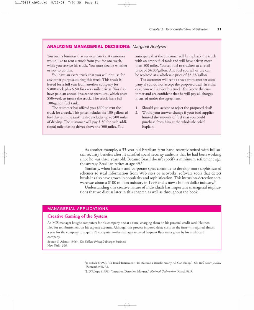
You own a business that services trucks. A customerwould like to rent a truck from you for one week,while you service his truck. You must decide whetheror not to do this.
You have an extra truck that you will not use forany other purpose during this week. This truck isleased for a full year from another company for$300/week plus $.50 for every mile driven. You alsohave paid an annual insurance premium, which costs$50/week to insure the truck. The truck has a full100-gallon fuel tank.
The customer has offered you $600 to rent thetruck for a week. This price includes the 100 gallons offuel that is in the tank. It also includes up to 500 milesof driving. The customer will pay $.50 for each addi-tional mile that he drives above the 500 miles. You
anticipate that the customer will bring back the truckwith an empty fuel tank and will have driven morethan 500 miles. You sell fuel to truckers at a retailprice of $4.00/gallon. Any fuel you sell or use canbe replaced at a wholesale price of $3.25/gallon.
The customer will rent a truck from another com-pany if you do not accept the proposed deal. In eithercase, you will service his truck. You know the cus-tomer and are confident that he will pay all chargesincurred under the agreement.
1. Should you accept or reject the proposed deal?2. Would your answer change if your fuel supplier
limited the amount of fuel that you could purchase from him at the wholesale price? Explain.
8P. Fritsch (1999), “In Brazil Retirement Has Become a Benefit Nearly All Can Enjoy,” The Wall Street Journal(September 9), A1.
9J. D’Allegro (1999), “Intrusion Detection Matures,” National Underwriter (March 8), 9.
MANAGERIAL APPLICATIONS
Creative Gaming of the SystemAn MIS manager bought computers for his company one at a time, charging them on his personal credit card. He thenfiled for reimbursement on his expense account. Although this process imposed delay costs on the firm—it required almosta year for the company to acquire 20 computers—the manager received frequent flyer miles given by his credit cardcompany.Source: S. Adams (1996), The Dilbert Principle (Harper Business:New York), 326.
bri75829_ch02.qxd 8/13/08 7:04 PM Page 21

22 Part 1 Basic Concepts
Graphical ToolsEconomists often employ a set of graphical tools to illustrate how individuals makechoices. These tools distinguish between the preferences (level of satisfaction) that theindividual associates with each potential opportunity and the set of feasible opportuni-ties that an individual faces. We use these tools throughout this book. They also are usedin other courses within the typical business school curriculum, such as in finance,human relations, and marketing courses. Our intent is to introduce these tools so thatthe reader is comfortable using them in basic business applications. We subsequentlyapply the tools to analyze the problems at Merrill Lynch. The appendix to this chapterprovides a more detailed development of the economic theory of individual choice(commonly called the “Theory of Consumer Choice”).
Individual Objectives
Goods are things that people value. Goods include standard products like food andclothing, services like haircuts and education, as well as less tangible emotions such aslove of family and charity. The economic model of behavior posits that people acquiregoods that maximize their personal satisfaction, given their resource constraints (such asa limited income). Economists traditionally use the term utility in referring to personalsatisfaction.
To provide a more detailed analysis of how people make choices, economists repre-sent an individual’s preferences by a utility function. This function expresses the relationbetween total utility and the level of goods consumed. The individual’s objective is tomaximize this function, given the resource constraints.10 This concept can be illustratedmost conveniently through a simple example where an individual cares about only twogoods. The insights from this two-good analysis can be extended readily to the case ofadditional goods such as food, housing, clothing, respect, and charity.
Suppose that Dominique Lalisse values only food and clothing. In general form, hisutility function can be written as follows:
� �Utility � F(Food, Clothing) (2.1)
Dom prefers more of each good—thus, his utility rises with both food and clothing. InDom’s case, his specific utility function is
Utility � Food1�2 � Clothing1�2 (2.2)
For instance, if Dom has 16 units of food and 25 units of clothing, his total utility is 20(that is, utility � 161�2 � 25 1�2 � 4 � 5 � 20). Dom is better off with 25 units of bothfood and clothing. Here, his utility is 25 (utility � 251�2 � 251�2 � 5 � 5 � 25).
Utility functions rank alternative bundles of food and clothing in the order of mostpreferred to least preferred, but they do not indicate how much one bundle is preferredto another. If the utility index is 100 for one combination of food and clothing and 200
10Clearly, most individuals do not actually consider maximizing a mathematical function when they make thesechoices. However, this formulation can provide useful insights into actual behavior to the extent that itapproximates how individuals make choices. Mathematicians have shown that if an individual’s behavior isconsistent with some basic “axioms of choice” (comparability, transitivity, nonsatiation, and willingness tosubstitute), the individual will make choices as if he or she were trying to maximize a mathematical function.
bri75829_ch02.qxd 8/13/08 7:04 PM Page 22

Chapter 2 Economists’ View of Behavior 23
for another, Dom will prefer the second combination. The second bundle does not nec-essarily make him twice as well off as the first bundle.11 Neither does this formulationallow one person’s utility of a bundle to be compared to another person’s utility.
Indifference Curves
Preferences implied by the utility function can be illustrated graphically throughindifference curves. An indifference curve pictures all combinations of goods that yieldthe same utility. Given his utility function in Equation (2.2), Dom is indifferent be-tween either 16 units of food and 25 units of clothing or 25 units of food and 16 unitsof clothing. Both combinations yield 20 units of utility, and hence are on the sameindifference curve. Figure 2.1 shows two of Dom’s indifference curves. For example, ifgiven a choice between any two points on curve 1, Dom would say that he does not carewhich one is selected—in either case, he obtains 8 units of utility.
The slope at any point along one of Dom’s indifference curves indicates how muchfood he would be willing to give up for a small increase in clothing (his utility remainsunchanged by this exchange).12 Standard indifference curves that illustrate trade-offs
4 16 25C
4
16
25
F
Quantity of clothing
Qua
ntity
of
food
Increasingutility
1: U = 8
2: U = 20
Figure 2.1 Indifference Curves
These indifference curves picture allcombinations of food and clothingthat yield the same amount of utility.The specific utility function in thisexample is U � F1�2 � C1�2, where Fis food and C is clothing. Northeastmovements are utility-increasing.Indifference curve 2 represents allcombinations of food and clothingthat yield 20 units of utility, whereascurve 1 pictures all combinationsthat yield 8 units of utility. Otherindifference curves could be drawnfor different levels of utility.
11This is like rankings on a test—an individual who scores in the 80th percentile is not twice as smart as one fromthe 40th.
12Recall that the slope of a line is a measure of steepness, defined as the increase or decrease in height per unit ofdistance along the horizontal axis. Slopes of curves are found geometrically by drawing a line tangent to the curveat the point of interest and determining the slope of this tangent line. The slope at a point along one of Dom’sindifference curves indicates how the quantity of food changes for small changes in the amount of clothing inorder to hold utility constant. Since by definition Dom is indifferent to this exchange (he remains on the sameindifference curve), he is willing to make the exchange.
bri75829_ch02.qxd 8/13/08 7:04 PM Page 23
24 Part 1 Basic Concepts
between two goods have negative slopes. If Dom obtains a smaller amount of one goodsuch as clothing, the only way he can be equally as well off is to obtain more of anothergood like food. If at a point along an indifference curve the slope is �2, Dom is willingto give up 2 units of food to obtain 1 unit of clothing. Alternatively he is willing to giveup 1�2 unit of clothing to obtain 1 unit of food. This willingness to substitute hasimportant implications, which we discuss below.
North and east movements in graphs like Figure 2.1 are utility-increasing. Holdingthe amount of food constant, utility increases by increasing clothing (an eastward move-ment). Holding the amount of clothing constant, utility increases by increasing theamount of food (a northward movement). Thus, in Figure 2.1, Dom would rather be onindifference curve 2 than on 1. He obtains 20 units of utility rather than 8.
Economists typically picture indifference curves as convex to the origin (they bow in,as in Figure 2.1). Convexity implies that if Dom has a relatively large amount of food,he would willingly exchange a relatively large quantity of food for a small amount ofadditional clothing. Thus, the indifference curves in Figure 2.1 are steep when the levelof food is high relative to the level of clothing. In contrast, if he has a relatively largeamount of clothing, he would be willing to substitute only a small amount of food foradditional clothing. Correspondingly, the indifference curves in Figure 2.1 flatten asDom has less food and more clothing. The behavior implied by the convexity of indif-ference curves is consistent with the observed behavior of many individuals—most peo-ple purchase balanced combinations of food and clothing.
Opportunities and Constraints
Dom would like more of both food and clothing. Unfortunately, he faces a budget con-straint that limits his purchases. Suppose that he has an income of I and the prices perunit of food and clothing are Pf and Pc , respectively. Since he cannot spend more thanI, his consumption opportunities are limited by the following constraint:
I � Pf F � PcC (2.3)
where F and C represent the units of food and clothing purchased. This budget con-straint indicates that only combinations of food and clothing that cost no more than Iare feasible. Rearranging terms, this constraint can be written as
F � I�Pf � (Pc�Pf )C (2.4)
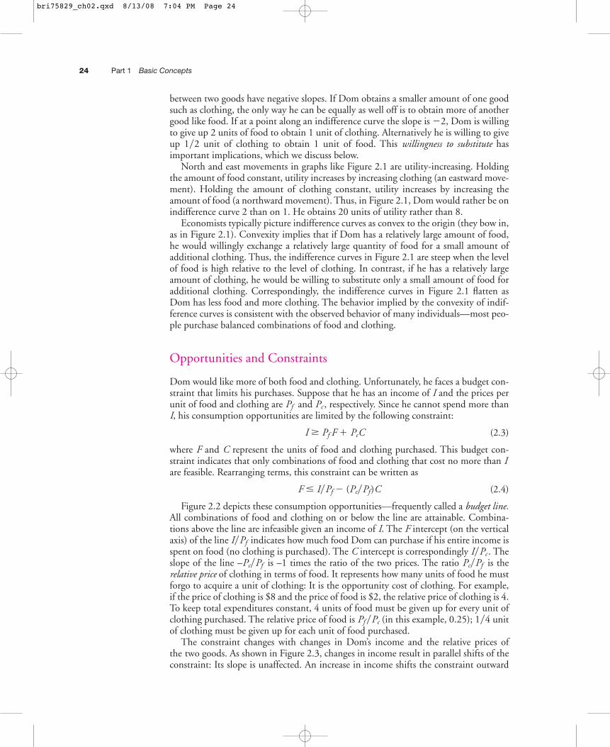
Figure 2.2 depicts these consumption opportunities—frequently called a budget line.All combinations of food and clothing on or below the line are attainable. Combina-tions above the line are infeasible given an income of I. The F intercept (on the verticalaxis) of the line I�Pf indicates how much food Dom can purchase if his entire income isspent on food (no clothing is purchased). The C intercept is correspondingly I�Pc . Theslope of the line –Pc�Pf is –1 times the ratio of the two prices. The ratio Pc�Pf is therelative price of clothing in terms of food. It represents how many units of food he mustforgo to acquire a unit of clothing: It is the opportunity cost of clothing. For example,if the price of clothing is $8 and the price of food is $2, the relative price of clothing is 4.To keep total expenditures constant, 4 units of food must be given up for every unit ofclothing purchased. The relative price of food is Pf �Pc (in this example, 0.25); 1�4 unitof clothing must be given up for each unit of food purchased.
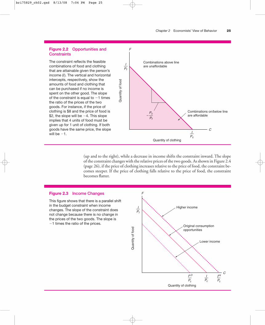
The constraint changes with changes in Dom’s income and the relative prices ofthe two goods. As shown in Figure 2.3, changes in income result in parallel shifts of theconstraint: Its slope is unaffected. An increase in income shifts the constraint outward
bri75829_ch02.qxd 8/13/08 7:04 PM Page 24
Chapter 2 Economists’ View of Behavior 25
IPf
IPc
C
Pf
Pc
F
Combinations above lineare unaffordable
Combinations on/below lineare affordable
Qua
ntity
of f
ood
Quantity of clothing
–
Figure 2.2 Opportunities andConstraints
The constraint reflects the feasiblecombinations of food and clothingthat are attainable given the person’sincome (I). The vertical and horizontalintercepts, respectively, show theamounts of food and clothing thatcan be purchased if no income isspent on the other good. The slopeof the constraint is equal to �1 timesthe ratio of the prices of the twogoods. For instance, if the price ofclothing is $8 and the price of food is$2, the slope will be �4. This slopeimplies that 4 units of food must begiven up for 1 unit of clothing. If bothgoods have the same price, the slopewill be �1.
IPc
IPf
C
F
Lower income
Original consumptionopportunities
Higher income
Quantity of clothing
Qua
ntity
of f
ood
IHI
Pc
ILO
Pc
Figure 2.3 Income Changes
This figure shows that there is a parallel shiftin the budget constraint when incomechanges. The slope of the constraint doesnot change because there is no change inthe prices of the two goods. The slope is �1 times the ratio of the prices.
(up and to the right), while a decrease in income shifts the constraint inward. The slopeof the constraint changes with the relative prices of the two goods. As shown in Figure 2.4(page 26), if the price of clothing increases relative to the price of food, the constraint be-comes steeper. If the price of clothing falls relative to the price of food, the constraintbecomes flatter.
bri75829_ch02.qxd 8/13/08 7:04 PM Page 25

26 Part 1 Basic Concepts
Individual Choice
Within this economic framework, Dom’s goal is to maximize utility given his opportu-nities. Utility is maximized at the point of tangency between the constraint and an in-difference curve.13 Figure 2.5 portrays the optimal choice. Dom could choose pointslike b and c on indifference curve 1. However, point a on curve 2 yields greater satisfac-tion and thus is preferred. Dom would prefer to be at any point on curve 3. Yet, thesepoints are unattainable given his income.
This graphical solution to Dom’s choice problem has a simple intuitive interpreta-tion. At the point of tangency, the indifference curve and the constraint have equalslopes. Recall that the slope of the indifference curve represents Dom’s willingness totrade food for clothing, whereas the slope of the constraint represents the terms of tradeavailable in the marketplace. At the optimal choice, the willingness and ability to tradeare equal. At other feasible combinations of food and clothing, Dom’s utility could beincreased by making substitutions. For instance, if Dom were at a point where he waswilling to trade 5 units of food for 1 unit of clothing and if the relative price of clothingwere 4 (the slope of the indifference curve is steeper than the constraint), Dom wouldbe better off purchasing less food and more clothing. (He is willing to trade 5 units offood for one unit of clothing, but only must forgo 4 units of food to obtain 1 unit ofclothing in the marketplace.) Alternatively, if Dom were at a point where he was onlywilling to forgo 1 unit of food for 1 unit of clothing (the slope of the indifference curveis flatter than the constraint), he would be better off purchasing more food and lessclothing—since he receives 5 units of food for each unit of clothing forgone.
C
IPf
F
Increase in the price of clothing
Original consumptionopportunities
Decrease in the price of clothing
Quantity of clothing
Qua
ntity
of f
ood
IPc
IPc
LOI
PcHI
Figure 2.4 Price Changes
This figure shows how hisconsumption opportunities changewith changes in the price of clothing.The slope of the line is �(Pc�Pf).Thus, an increase in the price ofclothing (from Pc to Pc
HI ) produces asteeper line, while a decrease (fromPc to Pc
LO ) produces a flatter line.Changes in the price of food alsoaffect the slope of the line.
13For simplicity, we ignore the possibility of corner solutions—the points where the budget constraint intersectsthe axes. With corner solutions, the individual spends all income on only one good.
bri75829_ch02.qxd 8/13/08 7:04 PM Page 26

Chapter 2 Economists’ View of Behavior 27
Earlier in this chapter, we discussed how marginal analysis is the cornerstone of mod-ern economics. It is important to understand that the graphical tools presented in thissection depict marginal analysis. In marginal analysis, individuals take actions as long astheir incremental benefits are greater than their incremental costs. Our graphical analy-sis of individual choice corresponds to this decision rule. The relative price ratio, PC�PF,is the marginal cost of a unit of clothing, expressed as units of food—the units of foodthat are forgone is the opportunity cost of an additional unit of clothing. Similarly, theopportunity cost of an additional unit of food is PF�PC units of clothing. The slope ofthe indifference curve reflects the marginal benefit of an additional unit of clothing ex-pressed as units of food. For example, if Dom is willing to trade 5 units of food for 1 unitof clothing (slope of the indifference curve � �5), his marginal benefit of one addi-tional unit of clothing must equal the utility from 5 units of food. Similarly, his mar-ginal benefit of a unit of food is equivalent to .2 units (1�5) of clothing. If Dom is notat the point of tangency between the indifference curve and the budget line, the mar-ginal benefit of trading one good for the other must be greater than the marginal cost.Suppose Dom is willing to trade 5 units of food for 1 unit of clothing, but only has totrade 2 units of food for 1 unit of clothing in the marketplace. In this case, Dom shouldtrade food for clothing since the marginal (incremental) benefit is greater than the mar-ginal (incremental) cost. At the optimum (point of tangency) the marginal benefit ofconsuming 1 more unit of either good is equal to the marginal cost and there is no rea-son to make additional trades.
Changes in Choice
Dom’s consumption opportunities will change whenever prices or income change. Con-sequently, he will make different choices. Recall that changes in relative prices alter theslope of the constraint. When the relative price of a good increases, individuals typically
C *
F
F *
b
a
c1
2
3
Quantity of clothingQ
uant
ity o
f foo
d
C
Figure 2.5 Optimal Choice
The individual is best off by choosingpoint a where the constraint is tangentto indifference curve 2. This optimalcombination of food and clothing, F* andC*, yields higher utility than other feasiblealternatives (for example, points b and c).The individual would prefer points onindifference curve 3, but these pointsare infeasible given his consumptionopportunities.
bri75829_ch02.qxd 8/13/08 7:04 PM Page 27

28 Part 1 Basic Concepts
choose less of that good.14 Figure 2.6 shows how Dom will purchase less food as its rela-tive price increases—food is more expensive and so less attractive than it was at a lowerprice. Generally the amount of clothing purchased can go either up or down; it dependson the location of the new tangency point. (Given the particular utility function assumedin this example, the amount of clothing purchased remains unchanged.) Even thoughthe price of clothing is relatively more attractive, the increase in food prices can limitavailable income so as to reduce the amount purchased of both goods. Changes inDom’s income cause parallel shifts in the constraint and will change his optimal choice.In Chapter 4, we examine in more detail how changes in income and prices affect con-sumption choices. The appendix to this chapter contains a more detailed analysis of theeffects of price changes on individual choice.
Choices also change if preferences change. Now changes in preferences undoubtedlyoccur. (Do you really believe that Toys ‘R’ Us will have any difficulty satisfying thedemands for toys that were highly popular in past years, such as Teenage Mutant NinjaTurtle action figures, Tomaguchi virtual pets, Tickle-Me-Elmo dolls, or Pokemon Cardsnext Christmas?) Yet, economists rarely focus on such explanations. Economics has lit-tle theory to explain what might cause preferences to change. And since a large premiumis placed on operationalism in managerial economics, preference-based explanationsgenerally are appealed to only after other potential explanations are exhausted. In asense, these preference-based explanations are too easy—they work too well. Virtuallyany observed behavior could be explained by appealing to preferences: Why did theconsumption of frozen yogurt increase relative to that of ice cream? People’s preferenceschanged so that more frozen yogurt and less ice cream was demanded. But an observed
C *C
F
F0
Consumption opportunities after increase in price of food
Original consumption opportunities
Quantity of clothing
Qua
ntity
of f
ood
*
F1*
Figure 2.6 Optimal Choice and PriceChanges
This figure shows how the optimal choicechanges with an increase in the price offood. In this example, the individualchooses less food (F1* rather than F0*). Thisis the typical case—usually, an individualwill purchase less of a good when its priceincreases. Due to the particular utilityfunction used in this example, the amountof clothing purchased remains unchanged(C*). More generally, the amount of clothingpurchased can go either up or down. Itdepends on the location of the newtangency point.
14Although in principle some individuals might purchase more of a good if its price increases, this outcome israrely observed.
bri75829_ch02.qxd 8/13/08 7:04 PM Page 28
Chapter 2 Economists’ View of Behavior 29
ANALYZING MANAGERIAL DECISIONS: Consumer Choice and Graphical Tools
You are a manager for a company that bottles andsells wine in two different countries. You charge thesame price for a bottle of wine in both countries. Yet,your wine sales are much higher in one country thanthe other. Your boss asks you to develop an explana-tion for the differences in wine sales between the twocountries and to develop a plan to sell more wine inthe country with low wine consumption.
Population sizes and family incomes in the twocountries are very similar. You also know that eachcountry imposes a per bottle tax on wine.
Begin by providing a plausible economic explana-tion (focusing on constraints) for the differences inwine sales in the two countries. Illustrate your expla-nation by using indifference curves and budget linesfor representative consumers from the two countries.What data would you want to determine if yourexplanation is likely to be correct? Are there other
plausible explanations for the differences in wineconsumption? Are there ways to determine whichof these explanations is most likely to be driving thedifferences in consumption?
1. Suppose that your economic explanation islikely to be correct and that your company willnot allow you to lower the price per liter thatyou charge for wine in the two countries. Discuss at least two potential actions that youmight take to sell more wine in the countrywith low demand.
2. Now provide a potential preference-based explana-tion for the differences in wine sales. Supposethat this explanation is correct. Discuss whetherthere are likely to be feasible policies that youcould use to increase wine sales in the countrywith the low demand.
reduction in consumption could have been “explained” just as readily. Without a deeperunderstanding of why preferences change, one is left “explaining” everything but withan analysis that allows you to predict nothing.
Ultimately, the managerial usefulness of this analysis comes from its power to iden-tify policy instruments that have a predictable impact on the problems at hand. Acrossa broad array of problems, assuming that underlying preferences are reasonably stableand analyzing the impact of changes in opportunities and constraints regularly will yieldimportant managerial insights and identify productive managerial tools.
Motivating Honesty at Merrill LynchOften, economists focus on consumption goods such as food and clothing. This focus isnatural given the interests economists have in understanding consumer behavior. Yet thisanalysis can be extended easily to consider other goods that people care about, such as loveand respect.15 Such an extension can be used to analyze the problem at Merrill Lynch.
Suppose that Susan Chen, like other analysts at Merrill Lynch, values two goods—money and integrity. Her utility function is
� �Utility � F (Money, Integrity) (2.5)
Money is meant to symbolize general purchasing power; it allows the purchase of goodssuch as food, clothing, and housing. Integrity is something Sue values for its own sake—
15G. Becker (1993), “Nobel Lecture: The Economic Way of Looking at Behavior,” Journal of Political Economy101, 385–409.
bri75829_ch02.qxd 8/13/08 7:04 PM Page 29

30 Part 1 Basic Concepts
being honest in her dealings with other people provides Sue with satisfaction and shevalues it for that reason.
Suppose that integrity can be measured on a numerical scale with Sue preferringhigher values. For example, 5 units of integrity provide more utility than 4 units ofintegrity. (In actuality, measuring a good like integrity on a numerical scale might bequite difficult. Yet this complication does not limit the qualitative insights that we canderive from the analysis.)
Merrill paid its stock analysts an annual bonus that was based partly on the analyst’scontribution to the investment banking side of the business (e.g., the firm’s underwrit-ing activities). If Sue were completely honest and rated a company as a poor investment,the management of that company might take its investment banking business to an-other firm. The resulting loss in Merrill’s investment banking revenue would reduceSue’s annual bonus. This bonus scheme thus confronts Sue with a trade-off. She can behonest and derive satisfaction from maintaining her integrity, or she can be dishonest inher rating of the stock and obtain a higher bonus. (She also might consider the futureeffects on her income from developing a good or bad reputation as an investment ana-lyst. However, the analysis in this chapter is framed in a simple one-period context anddoes not consider monetary returns from developing a good reputation. In subsequentchapters we extend the analysis and consider such multiperiod effects.)
Figure 2.7 depicts Sue’s implied opportunities. This constraint shows the maximumcombinations of income and integrity that are feasible given the compensation planand conditions at the company.16 If Sue sacrifices all integrity, she earns $max a year. If
IcI
$
$max
$min
Quantity of integrityIn
com
e (in
dol
lars
)
Figure 2.7 Nature of Opportunities Facing anAnalyst at Merrill Lynch
The constraint depicts the maximum amounts ofmoney and integrity that are possible for the analystgiven the bonus plan and conditions at the company.If the analyst sacrifices all integrity and recommendsstocks even if they are poor investments, theemployee earns a maximum of $max a year. Investmentbanking business is lost if the analyst gives objectiveadvice and rates certain stocks as poor investments(selects a higher level of integrity). Income is lowersince the analyst is paid a bonus based on investmentbanking revenues. Ic represents complete honesty.
16For simplicity, we draw the constraint as linear. Linearity is not necessary for our analysis. Also, we want toemphasize that we put dollars on the vertical axis only because it is a convenient general indication of value, notbecause money is more important than other things. We could illustrate Sue’s willingness to trade integrityagainst anything else Sue values, such as Big Macs, pianos, or pairs of jeans.
bri75829_ch02.qxd 8/13/08 7:04 PM Page 30

Chapter 2 Economists’ View of Behavior 31
she is scrupulously honest in her investment recommendations, she earns less (there isa positive floor on her income, $min, since her base salary does depend on the amountof investment banking business and her analysis undoubtedly will suggest recom-mending some of Merrill’s clients’ stocks). Intermediate options along the constraintare possible. While Sue would like to earn more than $max, higher income is not feasi-ble in this job.
Sue chooses the combination of integrity and income that places her on the highestattainable indifference curve. This choice occurs at the point of tangency between herindifference curve and the constraint. Sue ends up selecting relatively low amounts ofintegrity because the bonus plan adopted by Merrill’s management has made integrityexpensive. If Sue chooses more integrity, she must forfeit a relatively large amount ofincome.
Management can alter the opportunities Sue and her colleagues face by changing itscompensation plan. In the Merrill case, reducing the emphasis of investment bankingrevenue in determining the annual bonus reduces the gains from dishonest advice andthus flattens the constraint. Changes in the slope of the constraint result in a differenttangency point and hence a different choice. Figure 2.8 shows how Sue’s optimalchoice changes when the emphasis on investment banking revenue is decreased.17 Theresult is more honest behavior. In essence, Sue “purchases” more integrity because it
$
$1*
I1* I2*
Case 2
Case 1I
Inco
me
(in d
olla
rs)
Quantity of integrity
$2*
Figure 2.8 Optimal Choices of an Analystat Merrill Lynch under Two DifferentCompensation Plans
Case 1 reflects the original compensation plan. Inthis case, compensation includes a high bonusbased on investment banking revenues and theconstraint is relatively steep. In Case 2, the firmreduces the emphasis on investment bankingrevenues in compensating analysts. The slope of theconstraint is flatter. The result is that the individualchooses a higher level of integrity in Case 2 than inCase 1.
17We have altered the compensation scheme in a manner that places Sue on the same indifference curve. Ourrationale for doing this is as follows: Merrill Lynch must provide Sue with sufficient utility to retain her at thefirm. Below this level of utility, Sue will quit and work elsewhere. Merrill Lynch is unlikely to want to pay Suemore than this minimum utility because it reduces firm profits. Thus, Merrill Lynch has an incentive to adjustcompensation in a manner that keeps her on the same indifference curve. Sue’s indifference curve in Figure 2.8can be viewed as this “reservation” utility. These issues are covered in more detail in Chapter 14.
bri75829_ch02.qxd 8/13/08 7:04 PM Page 31
32 Part 1 Basic Concepts
now is less expensive. Consistent with this analysis, Merrill, in its settlement with theState of New York, agreed to change the way it evaluated and compensated its analysts.Bonuses now are based on the quality of investment advice—not tied to investmentbanking business.
Managerial ImplicationsThis analysis illustrates how the economic framework can be used to analyze and addressmanagement problems. Managers are interested in affecting the behavior of individualssuch as employees, customers, union leaders, or subcontractors. Understanding whatmotivates individuals is critical. The economic approach views individual actions as theoutcomes of maximizing personal utility. People are willing to make substitutions (forexample, less leisure time for more income) so long as the terms of trade are advanta-geous. Managers can affect behavior by appropriately designing the opportunities facingindividuals. The design of the opportunities affects the trade-offs that individuals faceand hence their choices. For example, management can motivate employees through thestructure of compensation plans or customers through pricing decisions.
The outcome of individuals making economic choices is a function of both oppor-tunities and preferences. Individuals try to achieve their highest level of satisfactiongiven the constraints they face. Our discussion of management implications, however,intentionally focuses on opportunities and constraints, not preferences. As a manage-ment tool, the usefulness of focusing on personal preferences often is limited. It is diffi-cult to change what a person likes or does not like. Moreover, preferences rarely areobservable, and (as we noted earlier) virtually any observed change in choice can be“explained” as simply a matter of a change in personal tastes. For instance, a preference-based explanation as to why employees were dishonest at Merrill Lynch is that these em-ployees gained personal utility from being dishonest (or compared to employees at otherfirms, Merrill Lynch employees were willing to trade large amounts of personal integrityfor small financial rewards). This explanation is not very helpful in giving managementguidance on how to address the problem. It suggests that Merrill Lynch might try to fire
MANAGERIAL APPLICATIONS
Money and Job SatisfactionA former investment banker related that: “I recently decided to leave a promising career in an investment bank. The salarywas lavish but the working hours were inhuman, social or family life was nonexistent and the level of stress was intolerable.I’ve given it up for a job with a measly salary but one that’s interesting and personally satisfying and—guess what—I’venever been happier in my life.” In surveys of 400 executives by the Young President’s Organization, they admitted that the“pursuit of money consumed them,” yet played down the importance of money in career choices. Some equated wealthwith self-worth and others said, “There’s never enough.” However in attitude surveys, career-development programsconsistently top employees’ list of wants. Managers often insist they would never make career decisions primarily based onmoney. One manager ranks his family’s well-being and happiness as most important, but still appreciates the monetaryvalue of the job. One manager who received a large bonus said he will use the money for his children’s education, “It’s givenme a sense of relief. Now I can redirect some money to things we haven’t done or divert it into a retirement fund.” Thus,these executives clearly value things other than money and regularly make choices that trade off money for other things thatthey value.Source: H. Lancaster (1998), “Needy or Greedy?” The Wall Street Journal( June 30), B1; L. Kellaway (2007), “Do I Go for Money or Stay Put in aJob I Like?” Financial Times (March 21), 12.
bri75829_ch02.qxd 8/13/08 7:04 PM Page 32
Chapter 2 Economists’ View of Behavior 33
dishonest employees and replace them with employees who care more about personalintegrity. But the difficulty of observing personal preferences limits the viability of thisapproach. It would be difficult for Merrill Lynch to know if, as a group, its new hireswould be any less dishonest than the old employees. You cannot just ask applicants ifthey are honest—if they are not, they will have no qualms about claiming that they are.
The fact that individuals are clever and creative in limiting the effects of constraintsgreatly complicates management problems. Changing incentives will affect employeebehavior, though sometimes in a perverse and unintended manner. Consider two of theSoviet Union’s early attempts to adopt incentive compensation to motivate employees.To discourage taxi drivers from simply parking their cabs, they were rewarded for totalmiles traveled; to encourage additional production, chandelier manufacturers were re-warded on total volume of production—measured in kilograms. In response to these in-centive plans, Moscow taxi drivers began driving empty cabs at high speeds on highwaysoutside the city and chandelier manufacturers started producing such massive fixturesthat they literally would collapse ceilings. (It is less costly to make one 100-kilo chande-lier than five 20-kilo chandeliers; manufacturers also substituted lead for lighter-weightinputs.) Merrill Lynch initially adopted bonuses to motivate analysts to work harder andcooperate across business units. The dishonest behavior was a side effect that potentiallywas unanticipated when the plan was adopted.
In summary, the economic approach to behavior has important managerial implica-tions. The framework suggests that a manager can motivate desired actions by establish-ing appropriate incentives. However, managers must be careful because setting improperincentives can motivate perverse behavior.
MANAGERIAL APPLICATIONS
Medicare Creates Perverse Incentives for DoctorsDoctors do not care about money but are motivated by concerns about providing the best care for patients—right?Apparently many doctors and the major drug company employees do not think so. Perverse incentives among physiciansarguably have contributed to the problem of spiraling health care costs in the United States.
For years, Medicare (federal health program for the elderly) reimbursement policies allowed individual doctors to makehundreds of thousands of dollars a year in extra profits from the drugs they administered to patients in their offices (thedoctors would buy the drugs themselves and bill Medicare, rather than having the patients get them directly frompharmacies). For example, many cancer doctors earned over $1 million per year on drug sales alone. Because the profits ondifferent drugs varied enormously, doctors had incentives to prescribe medications with the highest profit margins. Somephysicians have acknowledged that they performed treatments that got them the best reimbursements, “whether or not thetreatments benefited patients.”
Drug companies were well aware of the Medicare policies and calculated the profits that doctors received fromprescribing specific drugs “down to the penny.” For example, in 1998 Schering-Plough told its sales representatives thatits drug for the treatment of bladder cancer could produce a profit for a physician of $2,373.84 per patient. Salesrepresentatives in turn made sure that doctors were well aware when their drugs were in the high profit category. Forinstance, a sales representative for AstraZeneca wrote in a letter to Arizona urologists, “DO THE MATH.”
Medicare changed its reimbursement policies in 2005 and reduced the profits that physicians could make on drug sales.At least some physicians have responded by shifting from drug intensive treatments to other treatments that have higherprofit margins. To quote one doctor, “People go where the money is, and you’d like to believe it’s different in medicine,but it’s really no different . . . as long as oncologists continue to be paid by the procedure instead of spending time withpatients, they will find ways to game the system.”Source: Alex Berensen (2007), “Incentives to Limit Any Savings in TreatingCancer,” nytimes.com (June 12).
bri75829_ch02.qxd 8/13/08 7:04 PM Page 33

34 Part 1 Basic Concepts
It is worth noting that economic analysis is limited in its ability to forecast the pre-cise choices of a given individual because individual preferences are largely unobserv-able. The focus is on aggregate behavior or on what the typical person tends to do. Forexample, an economist might not be very good at predicting the responses of individualemployees to a new incentive plan. An economist will be successful in predicting thatthe typical employee will work harder—and thus output for the group will rise—whencompensation is tied to output, than when a fixed salary independent of performance ispaid. Managers typically are interested in structuring an organizational architecture thatwill work well and does not depend on specific people filling particular jobs. Individu-als come and go, and the manager wants an organization that will work well as thesechanges occur. In this context, the economic framework is likely to be useful. To solvemanagement problems where the characteristics of a specific individual are more im-portant, other frameworks may be more valuable. For example, if the board is inter-viewing a potential new CEO, insights into that individual’s behavior derived frompsychology might be extremely useful.
Alternative Models of Behavior18
We have shown how the economic view of behavior can be used in managerial decisionmaking. We now discuss four other models that are commonly used by managers (eitherexplicitly or implicitly) to explain behavior. Our discussion of each of these models issimplified. The intent, however, is to capture the essence of a few of the more prominentviews that managers have about behavior and to illustrate how managerial decision
MANAGERIAL APPLICATIONS
Happy-Is-Productive versus Economic Explanations of the Hawthorne ExperimentsSeven productivity studies were conducted at Western Electric’s Hawthorne plant over the period 1924–1932. All sevenstudies focused on the response of assembly workers’ productivity when different aspects of the work environment weremanipulated (for example, length of break times and workday). Surprisingly, productivity rose virtually regardless of theparticular manipulation. For example, it is claimed that productivity increased whenever illumination of the work area waschanged, regardless of the direction of the change. When the lights were turned up, productivity increased, and when theywere turned down, productivity increased, as well. This result is known as the Hawthorne Effect and is among the mostdiscussed findings in psychology; it often is taken as support for the happy-is-productive model. The workers in theexperiment were given special attention and nonauthoritarian supervision relative to other workers at the plant. Also, theaffected workers’ views on the experiments were solicited by management, and the workers were given more responsibility.These actions, it has been argued, increased job satisfaction and performance.
Parsons (1974) presents evidence that the findings of the Hawthorne experiments also can be explained byaccompanying changes in the compensation system. Prior to the experiment, all workers were paid based on the output of agroup of about 100 workers. During the experiment, the compensation plan was changed to base pay on the output of onlyfive workers. In this case, a given worker’s output more directly affects her own pay, and economic theory predicts increasedoutput. Interestingly, the last of the original Hawthorne experiments observed workers where the compensation system wasnot changed. In that seventh experiment, there was no change in output.Source: H. Parsons (1974), “What Happened at Hawthorne?” Science 183,922–932.
18This section draws on W. Meckling (1976).
bri75829_ch02.qxd 8/13/08 7:04 PM Page 34

Chapter 2 Economists’ View of Behavior 35
making is affected by the particular view. We contrast these alternative views with theeconomic view and argue why the economic framework is a particularly useful tool formanagers.
Only-Money-Matters Model
Some people believe that the only important component of the job is the level of mon-etary compensation. But as we have already suggested, people have an incredibly broadrange of interests, extending substantially beyond money. And these interests are re-flected in a diverse array of activities. As examples, much of the work through the RedCross is undertaken by unpaid volunteers; people frequently choose early retirement,forgoing a regular paycheck to enjoy additional leisure time; riskier occupations com-mand higher pay in order to attract people into those jobs.
Some of this confusion can result from a misinterpretation of standard economicanalysis. Central to economics is the study of trade-offs (recall our discussion of indif-ference curves illustrating trade-offs between food and clothing). Economists frequentlyuse money as one of the goods being considered. But in these cases, money is merely aconvenient unit of value: It simply represents general purchasing power. Its use does notsuggest that only money matters.
Happy-Is-Productive Model
Managers sometimes assert that happy employees are more productive than unhappyemployees. Managers following this happy-is-productive model see as their goal thedesigning of work environments that satisfy employees. Psychological theories, suchas Maslow’s and Herzberg’s, are frequently used as guides in efforts to increase jobsatisfaction.19
A manager adhering to the happy-is-productive model might suggest that the prob-lem at Merrill Lynch was motivated by disgruntled employees who took out theirfrustrations on customers. This view implies that Merrill Lynch could reduce the prob-lem by promoting employee satisfaction through such actions as designing more inter-esting jobs, increasing the rates of pay, and improving the work environment. Happieremployees would be expected to provide customers with better investment advice.
The economic and happy-is-productive models do not differ based on what peoplecare about. The economic model allows individuals to value love, esteem, interestingwork, and pleasant work environments, as well as more standard economic goods such asfood, clothing, and shelter. The primary difference in the models is what motivates indi-vidual actions. In the happy-is-productive model, employees exert high effort when theyare happy. In the economic model, employees exert effort because of the rewards.
To contrast the two models, consider offering an employee guaranteed lifetimeemployment plus a large salary, which will be paid independent of performance. Thehappy-is-productive model suggests that the employee will be more productive,because the high salary and job security are likely to increase job satisfaction. The eco-nomic model suggests that the employee would exert less effort—since the employeereceives no additional rewards for working harder and will not be fired for exertinglow effort.
19F. Herzberg, B. Mausner, and B. Snyderman (1959), The Motivation to Work ( John Wiley & Sons: New York);and A. Maslow (1970), Motivation and Personality (Harper & Row: New York).
bri75829_ch02.qxd 8/13/08 7:04 PM Page 35

36 Part 1 Basic Concepts
Good-Citizen Model
Some managers subscribe to the good-citizen model. The basic assumption is that em-ployees have a strong personal desire to do a good job; they take pride in their work andwant to excel. Under this view, managers have three primary roles. First, they need tocommunicate the goals and objectives of the organization to employees. Second, theymust help employees discover how to achieve these goals and objectives. Finally, man-agers should provide feedback on performance so that employees can continue toimprove their efforts. There is no reason to have incentive pay, since individuals areinterested intrinsically in doing a good job.
This view suggests that the problems at Merrill Lynch occurred because employeesmisunderstood what was good for the company. Employees might have thought thatincreasing investment banking revenues was in the company’s best interests, even if itrequired a certain amount of dishonesty. Under the good-citizen view, the managementof Merrill Lynch could motivate employee honesty by clearly communicating to its an-alysts that Merrill Lynch would be better off in the long run if they did not deceive theircustomers. Managers might be instructed to hold a series of analyst meetings to stressthe value of honesty and objective investment advice.
In the good-citizen model, employees place the interests of the company first. Thereis never a conflict between an employee’s personal interest and the interest of thecompany. In contrast, the economic model posits that employees maximize their ownutility. Potential conflicts of interest often arise. The economic view predicts that pleasfrom Merrill Lynch management that analysts be more honest would have little effecton behavior unless they also changed the reward system to make it in the interests ofanalysts to be more honest.
Product-of-the-Environment Model
The product-of-the-environment model argues that the behaviors of individuals arelargely determined by their upbringings. Some cultures and households encourage pos-itive values in individuals, such as industry and integrity, whereas others promote nega-tive traits, such as laziness and dishonesty. This model suggests that Merrill Lynch haddishonest analysts. A response would have been to fire these employees and replace themwith honest analysts from better backgrounds.
MANAGERIAL APPLICATIONS
Culture and BehaviorIn Tokyo, lost cell phones, umbrellas, and cash regularly find their way to the Tokyo Metropolitan Police Lost and FoundCenter—the Japanese are scrupulous about turning in found articles. In 2002 the center handled $23 million in cash and330,000 umbrellas. The system traces its roots to a code written in 718. Lost goods, animals, and servants had to be handedover to a government official within five days of being found. Not handing over found objects was severely punished. In1733 two officials who kept a parcel of clothing were led around town and executed. Current law gives the finder seven daysto turn in found goods. If the item is reclaimed, the finder is entitled to a reward (5 to 20 percent). If the item is notreclaimed within six months, the finder can claim it.
The most commonly reclaimed item is a cell phone—about 75 percent are returned. The least reclaimed are umbrellasat 0.3 percent.Source: N. Onishi (2004), “Never Lost, but Found Daily,” New York Times(January 8), A1.
bri75829_ch02.qxd 8/13/08 7:04 PM Page 36
Chapter 2 Economists’ View of Behavior 37
Which Model Should Managers Use? Behavior is a complex topic. No behavioral model is likely to be useful in all contexts.For example, the economic model is unlikely to be helpful in predicting whether a givenindividual will prefer a red shirt to a blue shirt (selling at the same price). But our focusis on managerial decision making. In this context, there are reasons to believe that theeconomic model is particularly useful.
Managers are frequently interested in fostering changes in behavior. For example,managers want consumers to buy more of their products, employees to exert moreeffort, and labor unions to accept smaller wage increases. In contrast to other models,the economic framework provides managers with concrete guidance on how to alterbehavior. Desired behavior can be encouraged by changing the feasible opportunitiesfacing the decision maker. For example, incentive compensation can be used to motivateemployees, and price changes can be used to affect consumer behavior.
There is ample evidence to support the hypothesis that this economic framework isuseful in explaining changes in behavior. The most common example is that consumerstend to buy fewer products at higher prices. The evidence suggests that the model is alsouseful in explaining aspects of behavior in many other contexts, including voting; theformation, dissolution, and structure of families; drug addiction; and the incidence ofcrime.20
The good-citizen model appears less successful in predicting behavior in businesssettings. Management would be an easy task if employees would work harder and pro-duce higher-quality products simply on request. The happy-is-productive model alsohas material limitations. Most importantly, the existing evidence suggests that there islittle relation between job satisfaction and performance (see Scott’s “Criticisms of theHappy-Is-Productive Model” in the accompanying box). Happy employees are notnecessarily more productive. Sometimes, managers might want to follow the implica-tions of the product-of-the-environment model and fire employees with undesirabletraits. Yet, this approach is of limited use in solving most managerial problems. Also,given laws that limit discrimination, this approach can subject the firm to potentiallyserious legal sanctions.
The Economic Framework and Criminal BehaviorCriminals often are viewed as psychologically disturbed. Evidence, however, suggests that criminal behavior can beexplained, at least in part, by the economic framework. This framework predicts that a criminal will consider the marginalcosts and benefits of a crime and will commit the crime only when the benefits exceed the costs. Under this view, increasingthe likelihood of detection and/or the severity of punishment will reduce crimes. In a pioneering study, Issac Ehrlichexamined whether the incidence of major felonies varied across states with the expected punishment. He found that theincidence of robberies decreased about 1.3 percent in response to each 1 percent increase in the proportionate likelihood ofpunishment. The incidence of crime also decreased with the severity of the punishment. Since Ehrlich’s study, scholars haveconducted extensive research on this topic. In general, the results support the conclusion that the economic model plays auseful role in explaining criminal activity.Source: I. Ehrlich (1973), “Participation in Illegitimate Activities: ATheoretical and Empirical Investigation,” Journal of Political Economy81, 521–565.
ACADEMIC APPLICATIONS
20G. Becker (1993).
bri75829_ch02.qxd 8/13/08 7:04 PM Page 37
38 Part 1 Basic Concepts
Criticisms of the Happy-Is-Productive ModelW. Richard Scott summarizes some of the major concerns about the happy-is-productive model (sometimes referred to asthe human-relations movement):
Virtually all of these applications of the human-relations movement have come under severe criticism on bothideological and empirical grounds. Paradoxically, the human-relations movement, ostensibly developed to humanize thecold and calculating rationality of the factory and shop, rapidly came under attack on the grounds that it representedsimply a more subtle and refined form of exploitation. Critics charged that workers’ legitimate economic interests werebeing inappropriately deemphasized; actual conflicts of interest were denied and “therapeutically” managed; and the rolesattributed to managers represented a new brand of elitism. The entire movement was branded as “cow sociology” just ascontented cows were alleged to produce more milk, satisfied workers were expected to produce more output.
The ideological criticisms were the first to erupt, but reservations raised by researchers on the basis of empirical evidencemay in the long run prove to be more devastating. Several decades of research have documented no clear relation betweenworker satisfaction and productivity.
Source: W. Scott (1981), Organizations: Rational, Natural and OpenSystems (Prentice Hall: Englewood Cliffs, NJ), 89–90.
ACADEMIC APPLICATIONS
ANALYZING MANAGERIAL DECISIONS: Interwest Healthcare Corp.
Interwest Healthcare is a nonprofit organizationthat owns 10 hospitals located in three westernstates. Cynthia Manzoni is Interwest’s chief executiveofficer. Vijay Singh, Interwest’s chief financial officer,and the administrators of the 10 hospitals report toManzoni.
Singh is deeply concerned because the hospitalstaffs are not being careful when entering data intothe firm’s management information system. This datainvolves information on patient intake, treatment,and release. The information system is used to com-pile management reports such as those relating to thecosts of various treatments. Also, the system is usedto compile reports that are required by the federalgovernment under various grant programs. Singh rea-sons that without good information, the managementand government reports are less useful and potentiallymisleading. Moreover, the federal government peri-odically audits Interwest and might discontinue aidif the reports are deemed inaccurate. Thus, Singh isworried about the managerial implications and thepotential loss of federal funds.
Singh has convinced Manzoni that a problem exists.She also realizes the importance of an accurate systemfor both management planning and maintaining
federal aid. Six months ago, she invited the hospitaladministrators and staff members from the corporatefinancial office to a retreat at a resort. The purposewas to communicate to the hospital administratorsthe problems with the data entry and to stress theimportance of doing a better job. The meeting wasacrimonious. The hospital people accused Singh ofbeing a bureaucrat who did not care about patientservices. Singh accused the hospital staffs of not un-derstanding the importance of accurate reporting.By the end of the meeting, Manzoni thought that shehad a commitment by the hospital administrators toincrease the accuracy of data entry at their hospitals.However, six months later, Singh claims that theproblem is as bad as ever.
Manzoni has hired you as a consultant to analyzethe problem and to make recommendations thatmight improve the situation.
1. What are the potential sources of the problem?2. What information would you want to analyze?3. What actions might you recommend to increase
the accuracy of the data entry?4. How does your view of behavior affect how you
might address this consulting assignment?
bri75829_ch02.qxd 8/13/08 7:04 PM Page 38

Chapter 2 Economists’ View of Behavior 39
Decision Making under UncertaintyThroughout this chapter, we have considered cases where the decision maker has com-plete certainty about the items of choice. For instance, Dom Lalisse knew the exactprices of food and clothing, and Sue Chen knew the precise trade-off between integrityand compensation at Merrill Lynch. Decision makers, however, often face uncertainty.For instance, in choosing among risky investment alternatives (such as stocks andbonds), an individual must forecast the likely payoffs. Even so, there can be significantuncertainty about the eventual outcomes. The analysis presented in this chapter can beextended readily to incorporate decision making under uncertainty.21 A detailed analysisof decision making under uncertainty is beyond the scope of this book. This section in-troduces a few key concepts that we will use later in this book.
Expected ValueTaylor McClure sells real estate for RealCo. He receives a sales commission from his em-ployer. For simplicity, suppose that Taylor has three possible incomes for the year. In agood year, he sells many houses and earns $200,000, whereas in a bad year he earnsnothing. In other years, he receives $100,000. Probability refers to the likelihood that anoutcome will occur. In this example, each outcome is equally likely, and thus has a prob-ability of 1�3 of occurring. The expected value of an uncertain payoff is defined as theweighted average of all possible outcomes, where the probability of each outcome is usedas the weights. The expected value is a measure of central tendency—the payoff that willoccur on average. In our example, the expected value is:22
Expected value � (1�3 � 0) � (1�3 � 100,000) � (1�3 � 200,000) (2.6)� $100,000
VariabilityAlthough Taylor can expect average earnings of $100,000, his income is not certain. Thevariance is a measure of the variability of the payoff. It is defined as the expected valueof the squared difference between each possible payoff and the expected value. In thisexample, the variance is
Variance � 1�3(0 � 100,000)2 � 1�3(100,000 � 100,000)2 (2.7)�1�3(200,000 � 100,000)2
� 6.7 billion
The standard deviation is the square root of the variance:
Standard deviation � (6.7 billion)1�2 � $81,650 (2.8)
Variances and standard deviations are used as measures of risk. It does not really matterwhich we use, since one is a simple transformation of the other (higher standard deviationscorrespond to higher variances). In this example, we focus on the standard deviation—in
21For example, E. Fama and M. Miller (1972), The Theory of Finance (Dryden Press: New York), Chapter 5.22Note that the expected value need not equal one of the possible outcomes. As a weighted average, it can be
a value between outcomes. In this example, it happens to correspond to one of the possible outcomes,$100,000.
bri75829_ch02.qxd 8/13/08 7:04 PM Page 39
40 Part 1 Basic Concepts
part because the standard deviation is expressed in the same units as the mean, dollars (theunits for the variance would be dollars squared). Higher standard deviations reflect morerisk. An event with a definite outcome has a standard deviation of zero.
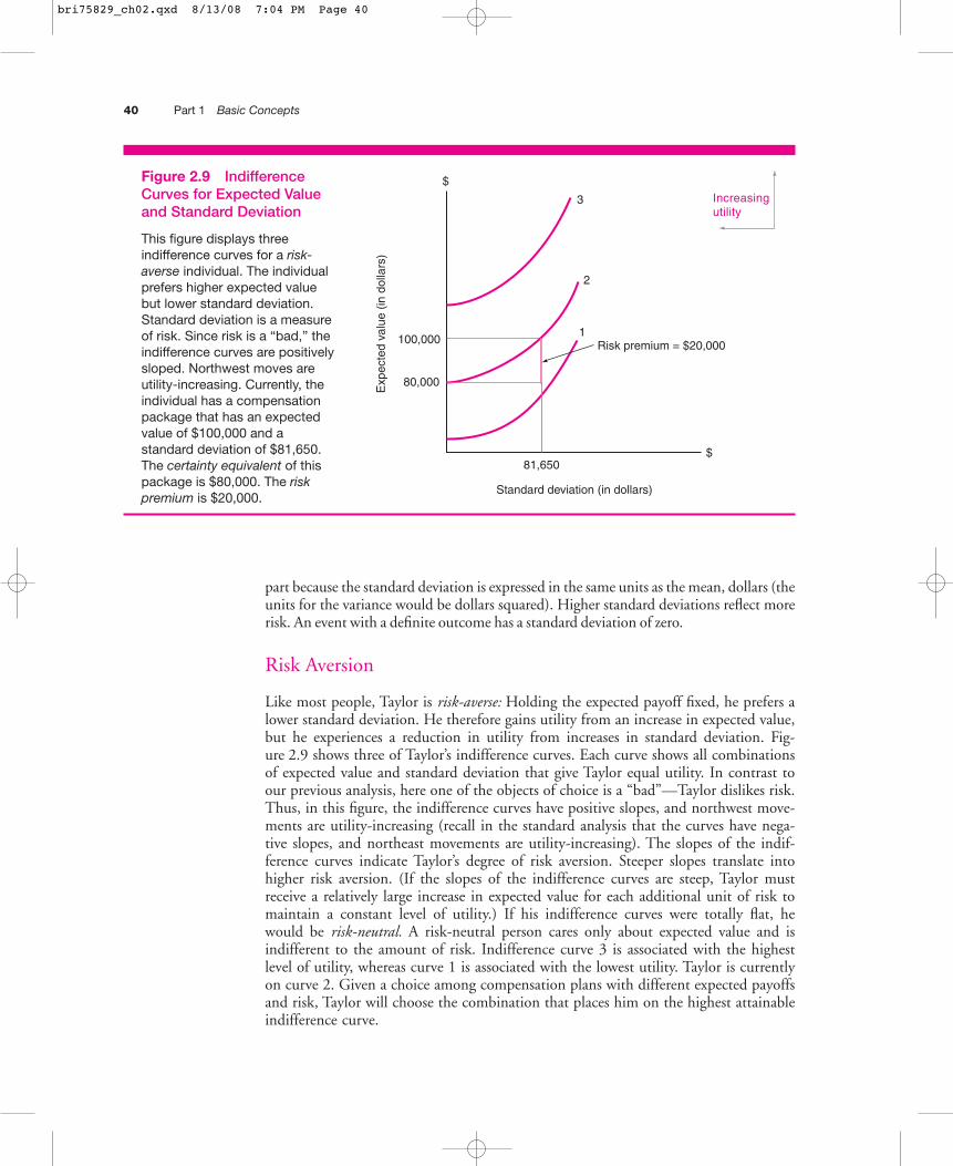
Risk Aversion
Like most people, Taylor is risk-averse: Holding the expected payoff fixed, he prefers alower standard deviation. He therefore gains utility from an increase in expected value,but he experiences a reduction in utility from increases in standard deviation. Fig-ure 2.9 shows three of Taylor’s indifference curves. Each curve shows all combinationsof expected value and standard deviation that give Taylor equal utility. In contrast toour previous analysis, here one of the objects of choice is a “bad”—Taylor dislikes risk.Thus, in this figure, the indifference curves have positive slopes, and northwest move-ments are utility-increasing (recall in the standard analysis that the curves have nega-tive slopes, and northeast movements are utility-increasing). The slopes of the indif-ference curves indicate Taylor’s degree of risk aversion. Steeper slopes translate intohigher risk aversion. (If the slopes of the indifference curves are steep, Taylor mustreceive a relatively large increase in expected value for each additional unit of risk tomaintain a constant level of utility.) If his indifference curves were totally flat, hewould be risk-neutral. A risk-neutral person cares only about expected value and isindifferent to the amount of risk. Indifference curve 3 is associated with the highestlevel of utility, whereas curve 1 is associated with the lowest utility. Taylor is currentlyon curve 2. Given a choice among compensation plans with different expected payoffsand risk, Taylor will choose the combination that places him on the highest attainableindifference curve.
$
Exp
ecte
d va
lue
(in d
olla
rs)
3
2
1Risk premium = $20,000
Standard deviation (in dollars)
81,650
80,000
100,000
Increasingutility
$
Figure 2.9 IndifferenceCurves for Expected Valueand Standard Deviation
This figure displays threeindifference curves for a risk-averse individual. The individualprefers higher expected valuebut lower standard deviation.Standard deviation is a measureof risk. Since risk is a “bad,” theindifference curves are positivelysloped. Northwest moves areutility-increasing. Currently, theindividual has a compensationpackage that has an expectedvalue of $100,000 and astandard deviation of $81,650.The certainty equivalent of thispackage is $80,000. The riskpremium is $20,000.
bri75829_ch02.qxd 8/13/08 7:04 PM Page 40

Chapter 2 Economists’ View of Behavior 41
Certainty Equivalent and Risk Premium
Figure 2.9 indicates that Taylor is indifferent between the risky commission scheme,which has an expected payoff of $100,000, and a certain income of $80,000. The$80,000 is Taylor’s certainty equivalent for the risky income stream—he is willing totrade the uncertain income of $100,000 for a certain income of $80,000. The differencebetween the expected value of the risky income stream and the certainty equivalent iscalled the risk premium. This $20,000 premium, which comes in the form of a higherexpected payoff, must be paid to keep Taylor indifferent between the risky incomestream and his certainty equivalent.
Suppose that Taylor receives a job offer from a competing real estate company thatwould pay him a fixed salary of $90,000 per year. Taylor considers the new job to be thesame as his current job in all dimensions other than the compensation plan. Taylor’scurrent compensation plan will not be sufficient to motivate him to continue to workfor RealCo. Even though his current plan has a higher expected payoff, he would preferthe certain $90,000 to RealCo’s risky commission plan. If RealCo wants to retain Taylor,it must offer him a compensation package that provides the same level of utility as the$90,000 for certain.
Risk Aversion and Compensation
Diversified shareholders, who invest in portfolios of companies, own much of the stockof large firms. Managers are often ill-diversified, having much of their human andfinancial capital invested in one firm. As we will discuss later in this book, this differencein diversification can lead to managers being overly risk averse in their investment deci-sions relative to those shareholders would prefer. Shareholders can induce managers to
ANALYZING MANAGERIAL DECISIONS: Risk Aversion versus Risk Taking
Lauren Arbittier decides to bet $2,000 on number 35of the roulette wheel in a Las Vegas casino. Almostimmediately she starts to question her decision.Lauren normally is a risk avoider who hardly evergambles. But she works at Trilogy Software wherethe CEO understands that taking risks and sufferingthe consequences are critical to the firm’s success. TheCEO wants to develop people who take chances.“You don’t win points . . . for trying.” Lauren is par-ticipating in Trilogy’s three-month training programfor all new recruits. It educates employees about,among other things, how to evaluate risky projects,not just to immediately accept or reject the projectbecause it is risky. The program also suggests toemployees that they will not be rewarded at Trilogy
unless they take risks. Thus, although Lauren doesnot like taking risks, working for Trilogy, she haseconomic incentives to do so.
There are at least three ways in which the Trilogytraining program might be effective: (1) It changesemployees’ preferences regarding risk bearing. (2) It more effectively identifies individuals with therisk to tolerances that Trilogy desires. (3) It bettercommunicates the consequences to Trilogy employeesof undertaking risky ventures. Discuss the likelyimportance of these three mechanisms.
SOURCE: E. Ramstad (1998), “High Rollers, How Trilogy SoftwareTrains Its Raw Recruits to Be Risk Takers,” The Wall Street Journal(September 21), A1.
bri75829_ch02.qxd 8/13/08 7:04 PM Page 41

42 Part 1 Basic Concepts
undertake more risky investment by adopting compensation plans that reward goodoutcomes, but that do not penalize bad outcomes heavily. The top management ofEnron (see Chapter 1) arguably went too far in this direction, inducing their managersto take too much risk (effectively transforming their behavior from risk averse to “riskloving”).23 We expand on this issue later in the book.
Summary In this chapter we summarize the way economists view behavior. In the economicmodel, individuals are seen as having unlimited wants but limited resources. They rankalternative uses of limited resources in terms of preference and choose the most preferredalternative. Individuals are clever in figuring out ways of maximizing their satisfaction(utility) in the face of resource constraints. Individuals are not necessarily selfish in thesense that they care only about their personal wealth: They also care about charity, fam-ily, religion, and society. They are not infallible supercomputers.
The opportunity cost of using a resource is the value of the resource in its best alterna-tive use. For example, the cost of having a manager use five hours to work on a project isthe value of the manager’s time in working on the next best alternative project. Economicdecision making requires careful consideration of the relevant opportunity costs.
Marginal costs and benefits are the incremental costs and benefits that are associatedwith a decision. In calculating marginal costs, it is important to use the opportunitycosts of the incremental resources. For example, in deciding whether to purchase a newlaptop computer, the marginal cost is its price and the marginal benefit is the value thatthe person places on the new computer. It is the marginal costs and benefits that areimportant in economic decision making. Action should be taken when the marginalbenefits are greater than the marginal costs. Sunk costs that are not affected by the decision(for example, unrecoverable funds previously spent on computers) are not relevant.
A utility function is a mathematical function that relates total utility to the amountsthat an individual has of whatever items the individual cares about (goods). Preferencesimplied by a utility function are pictured graphically by indifference curves. Indifferencecurves picture all combinations of goods that yield the same level of utility. Individualchoice involves maximizing utility given resource constraints. Graphically, the constraintdepicts all combinations of goods that are feasible to acquire; it defines the feasible con-sumption opportunities. The optimal choice is where the indifference curve is tangentto the constraint. At this point, the individual is at the highest level of utility possiblegiven the feasible opportunities.
Changes in opportunities result in changes in the optimal choice. An importantimplication is that managers can affect behavior by affecting constraints and opportuni-ties. Managers, however, have to be careful. Individuals are clever at maximizing theirutility, and establishing disfunctional incentives can have perverse consequences.
We contrast the economic model with other models of human behavior that man-agers often use. We argue that the economic model is often more useful than alternativemodels in managerial decision making.
The analysis in this chapter can be extended to the case where the decision makerfaces uncertainty about the items of choice. An example of decision making under un-certainty is choosing among risky investment alternatives. One concept that we will rely
23Most managers have risk-averse preferences (utility functions). Managerial actions, however, are a function of bothpreferences and constraints. Thus risk-averse preferences can be offset or reinforced by the design of the com-pensation plan. Compensation plans that limit the upside potential but not the downside induce less risky choices,whereas plans that limit the downside but not the upside induce more risky choices.
bri75829_ch02.qxd 8/13/08 7:04 PM Page 42

Chapter 2 Economists’ View of Behavior 43
on later in this book is risk aversion. When confronted with both a risky and a certainalternative having the same expected (or average) payoffs, a risk-averse person alwayswill choose the certain outcome. A risk premium must be offered to entice the person tochoose the risky alternative.
Throughout this chapter, we focus primarily on how managers might use the eco-nomic view to analyze and influence the behavior of employees. As we will see, theeconomic view is quite powerful and is useful in explaining behavior in a variety ofdifferent contexts.
Appendix Consumer ChoiceThe main text of this chapter provided a simple graphical analysis of individual choice.It introduced utility functions, indifference curves, and budget lines. It depicted the op-timal choice as the tangency between an indifference curve and the budget line wherethe willingness and ability to trade are equal. This simple analysis explained how theoptimal choice changes with changes in relative prices or income. This economic frame-work has important implications since managers often want to influence and/or predictthe behavior of individuals, such as customers and employees.
This appendix extends the economic framework of individual choice (commonlycalled consumer choice). Its intent is to provide a deeper and richer understanding of thisimportant model of behavior. This appendix also discusses how this model relates to animportant topic that is covered in more detail later in this book—demand functions.
Marginal UtilityA utility function expresses the relation between a person’s total utility and the level ofgoods consumed. Utility functions can take many forms. For illustration, suppose thatTom Morrell values only food and clothing and that his utility function is
U � FC (2.9)
where F is the units of food and C is the units of clothing that Tom consumes for theperiod. Notice, this simple utility function is multiplicative in both food and clothing.If Tom has no clothing, then no matter how much food he has, he has utility of zero.And likewise, if he has no food, then no matter has much clothing he has, his utilityagain is zero. If Tom’s consumption bundle consists of 20 units of both food and cloth-ing his utility is 400, while his utility is only 100 if he has 10 units of both goods. Tomprefers the first bundle, but he is not necessarily four times happier when he has20 units, rather than 10 units, of each good. The utility function provides an ordinalranking of consumption bundles—not a cardinal ranking where “absolute” comparisonscan be made.
Marginal utility measures the additional utility that is obtained by consuming oneadditional unit of a good, while holding all other goods constant. Marginal utility is animportant concept in economic analysis since optimizing individuals focus on the mar-ginal (incremental) benefits and costs in making consumption choices. Figure 2.10(page 44) graphs Tom’s utility as a function of food, while holding clothing constant at10 units. The equation for this graph is
U � 10F (2.10)
The marginal utility of food in this example is 10—for each additional unit of food thatTom consumes he receives 10 additional units of utility. More generally for any given
bri75829_ch02.qxd 8/13/08 7:04 PM Page 43

44 Part 1 Basic Concepts
quantity of clothing, C, the marginal utility of food is C (given Tom’s utility function).Similar logic implies that the marginal utility of clothing is F.24 We denote the marginalutilities for food and clothing by MUF and MUC , respectively.
Slope of an Indifference CurveNow that we have defined marginal utility, we can derive the slope of an indifferencecurve. Consider Tom’s indifference curve for U � 100. The equation for this indiffer-ence curve, which is pictured in Figure 2.11, is F � 100�C.25 Because all points on theindifference curve generate 100 units of utility, the total gain in utility associated withan increase in C must be balanced by an offsetting decline in utility from reduced con-sumption of F (as Tom moves along the curve):
MUC (�C ) � MUF (�F ) � 0, (2.11)
where �F and �C represent the changes in food and clothing. The first term in Equa-tion (2.11) represents the change in utility from changing the amount of clothing, whilethe second term represents the change in utility from changing the amount of food.These terms are equal in magnitude and of opposite sign along an indifference curve,and so total utility remains unchanged.
The slope of the indifference curve for a small change in C is given by (�F��C ).Rearranging Equation (2.11):
(�F��C ) � �(MUC�MUF) (2.12)Slope of the indifference curve � �(MUC�MUF)
0
Util
ity
50
100
150
200
250
300
350
400
1 3 5 7 9 11
Slope = 100/10 = 10
13 15 17 19 21 23 25 27 29 31 33 35Food (F )
1
10
Figure 2.10 Tom’s Utility as a Function of Food with Clothing Held Constant at 10 Units (U � 10F )
This figure displays Tom’s utility as a function of food with clothing held constant at 10 units. Marginal utilitymeasures the additional utility that is obtained by consuming one additional unit of a good, while holding allother goods constant. The marginal utility of F in this example is 10 (the slope of the line)—for each additional unit of F that Tom consumes he receives 10 additional units of utility.
24Note for the mathematically inclined: The marginal utility of any good X is equal to the partial derivative of theutility function with respect to X. In this example, the partial derivative with respect to F is C, and with respectto C is F. In this example, the marginal utility of each good is constant. More realistically, the marginal utility ofa good will eventually decline as the consumer continues to receive more of the good. We chose the utilityfunction in this example to simplify the presentation.
25The decision to place food on the y-axis is arbitrary. If we had placed clothing on the y-axis the equation for theindifference curve would be C � 100�F.
bri75829_ch02.qxd 8/13/08 7:04 PM Page 44
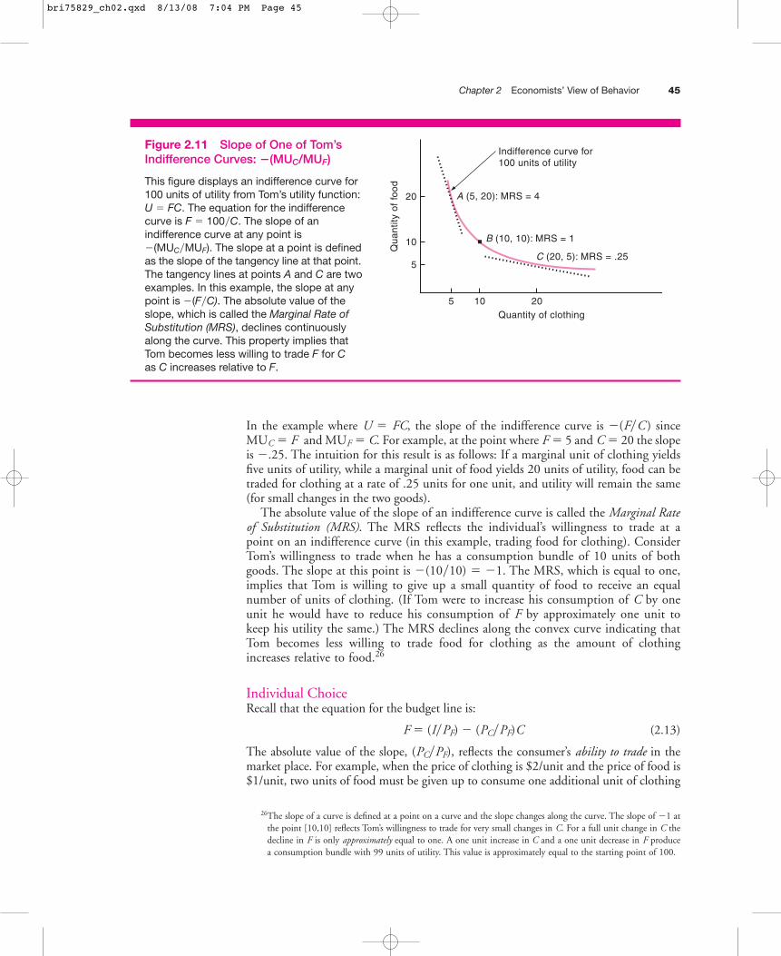
Chapter 2 Economists’ View of Behavior 45
In the example where U � FC, the slope of the indifference curve is �(F�C ) sinceMUC � F and MUF � C. For example, at the point where F � 5 and C � 20 the slopeis �.25. The intuition for this result is as follows: If a marginal unit of clothing yieldsfive units of utility, while a marginal unit of food yields 20 units of utility, food can betraded for clothing at a rate of .25 units for one unit, and utility will remain the same(for small changes in the two goods).
The absolute value of the slope of an indifference curve is called the Marginal Rateof Substitution (MRS). The MRS reflects the individual’s willingness to trade at apoint on an indifference curve (in this example, trading food for clothing). ConsiderTom’s willingness to trade when he has a consumption bundle of 10 units of bothgoods. The slope at this point is �(10�10) � �1. The MRS, which is equal to one,implies that Tom is willing to give up a small quantity of food to receive an equalnumber of units of clothing. (If Tom were to increase his consumption of C by oneunit he would have to reduce his consumption of F by approximately one unit tokeep his utility the same.) The MRS declines along the convex curve indicating thatTom becomes less willing to trade food for clothing as the amount of clothingincreases relative to food.26
Individual ChoiceRecall that the equation for the budget line is:
F � (I�PF) � (PC�PF)C (2.13)
The absolute value of the slope, (PC�PF), reflects the consumer’s ability to trade in themarket place. For example, when the price of clothing is $2/unit and the price of food is$1/unit, two units of food must be given up to consume one additional unit of clothing
5 10 20Quantity of clothing
5
10
20
Qua
ntity
of
food
Indifference curve for 100 units of utility
A (5, 20): MRS = 4
B (10, 10): MRS = 1
C (20, 5): MRS = .25
Figure 2.11 Slope of One of Tom’sIndifference Curves: �(MUC/MUF)
This figure displays an indifference curve for100 units of utility from Tom’s utility function:U � FC. The equation for the indifferencecurve is F � 100�C. The slope of anindifference curve at any point is�(MUC�MUF). The slope at a point is definedas the slope of the tangency line at that point.The tangency lines at points A and C are twoexamples. In this example, the slope at anypoint is �(F�C). The absolute value of theslope, which is called the Marginal Rate ofSubstitution (MRS), declines continuouslyalong the curve. This property implies thatTom becomes less willing to trade F for Cas C increases relative to F.
26The slope of a curve is defined at a point on a curve and the slope changes along the curve. The slope of �1 atthe point [10,10] reflects Tom’s willingness to trade for very small changes in C. For a full unit change in C thedecline in F is only approximately equal to one. A one unit increase in C and a one unit decrease in F producea consumption bundle with 99 units of utility. This value is approximately equal to the starting point of 100.
bri75829_ch02.qxd 8/13/08 7:04 PM Page 45
46 Part 1 Basic Concepts
(PC�PF � 2). The intercept (I�PF) indicates how many units of food could be purchasedif the entire budget is spent on food.
At the optimal consumption bundle the budget line is tangent to an indifferencecurve (which is the highest attainable indifference curve given the budget constraint).This condition implies that the MRS is equal to the ratio of the prices at the optimum.Since the MRS is equal to the ratio of the marginal utilities for the two goods:
MUC�MUF � PC�PF (2.14)
The left side of Equation (2.14) represents the willingness to trade, while the right sidereflects the ability to trade. At the point where the consumer is maximizing his utility(the optimum), the two are equal.
We can rearrange Equation (2.14) as follows:
MUC�PC � MUF�PF (2.15)
Equation (2.15) is an important and familiar result in consumer theory. It says that theconsumer’s utility is maximized when the budget is allocated among goods so that themarginal utility per dollar of expenditure is the same for each good. At any combinationwhere this condition does not hold, the consumer can be made better off by making fea-sible changes in the consumption bundle. For example, suppose Tom has an initial bun-dle where the marginal utility per dollar for clothing is 10 and for food is 20. Since he isgetting more utility per dollar from food, he should spend less money on clothing andmore on food. As he trades clothing for food, his marginal utility of clothing increaseswhile his marginal utility of food decreases. Tom will eventually reach the optimal con-sumption bundle where the marginal utility-to-price ratios are equal. Equation 2.15 re-flects a condition known as the equal marginal principle (the marginal utility per dollaris the same for all goods at the optimum).27 This principle reappears in various forms inthe economic analysis of both consumer and producer behavior.
Solving for the Optimal Consumption BundleSuppose that Tom has a budget of $100 and the prices of food and clothing are $1 and $2,respectively. How much of each good will he buy? This problem is straightforward since itinvolves two unknown variables (F and C ) and two independent equations. One equationis the optimality condition Equation (2.14); the second is the budget line Equation (2.13).
At Tom’s optimal choice, the MRS must equal the price ratio (i.e., MUC�MUF �PC�PF). Substituting the values for Tom’s marginal utilities yields:
F�C � 2 (2.16)C � F�2
Tom must also satisfy his budget constraint:
F � 100 � 2C. (2.17)
We can solve for the amount of food that Tom will purchase by substituting Equa-tion (2.16) into Equation (2.17):
F � 100 � 2 (F�2)F * � 50.
C * � 25 is found by substituting F * � 50 into Equation 2.16.
27This condition is also referred to as the “equimarginal principle.”
bri75829_ch02.qxd 8/13/08 7:04 PM Page 46

Chapter 2 Economists’ View of Behavior 47
At the optimal consumption bundle, Tom obtains 1,250 units of utility (25 � 50).He can increase his consumption of clothing by purchasing 26 units of clothing and48 units of food (26 � $2 � 48 � $1 � $100). However, this bundle would yield only1,248 units of utility (26 � 48). Alternatively, he could decrease his consumption ofclothing by one unit and increase his consumption of food by two units (C � 24;F � 52). This bundle also would produce only 1,248 units of utility. Indeed any feasi-ble alternative bundle would yield less than 1,250 units of utility.
The equal marginal principle holds at Tom’s optimal consumption bundle—the mar-ginal utility per dollar of expenditure (MUi�Pi) is 25 for both goods. This conditionimplies that Tom has no incentive to shift expenditures from one good to the other sinceboth goods yield the same marginal utility per dollar of spending.
The marginal utility of income is defined as the additional utility that the consumerreceives from one additional dollar of income. It can be shown that at the optimum, themarginal utility-to-price ratio for all goods is equal to the marginal utility of income. Forexample, if Tom’s income increases by $1, he could increase his utility by 25 units bypurchasing additional quantities of either good.
Demand FunctionsA demand function expresses the mathematical relation between the quantity demandedfor a product (how many units consumers will purchase) and the factors that determineconsumer choice (such as prices and income). In a more general setting than our simpleexample, the demand for clothing is likely to be affected by the price of clothing, con-sumer income, the prices of other products, and other variables (such as advertisingexpenditures). Managers care about consumer choice since a good understanding of thedemands for their products is important for making productive investment, pricing, ad-vertising, and other decisions. In subsequent chapters, we focus on aggregate demandfor a product (total demand across all consumers in the market) without directly tyingthe analysis back to individual consumer behavior as analyzed in this chapter. Neverthe-less, it is useful to recognize that aggregate demand for a given product can conceptuallybe derived from the framework presented in this appendix.
The derivation of Tom’s demand function for either food or clothing is particularlyeasy (given his utility function). Tom’s optimal consumption bundle is where his MRSequals the price ratio. In Tom’s case, this condition is:
F�C � PC�PF (2.18)
Tom’s total expenditures on either food or clothing is equal to the quantity purchased ofthe good times its price. By cross-multiplying Equation (2.18) we see that Tom’s expen-ditures on food and clothing are always equal:
(F � PF) � (C � PC) (2.19)
Equation (2.19) implies that Tom will always spend half his income on each good (thisresult is driven by his utility function). It follows that Tom’s total expenditures on cloth-ing are (C � PC) � I�2. Solving for C produces Tom’s demand function for clothing:
C � I�(2PC) (2.20)
This demand function implies that Tom will purchase more clothing as his income risesand less clothing as his income falls. His clothing purchases vary inversely with the priceof clothing.
In our example, Tom had an income of $100 and PC � $2/unit. Consistent withEquation (2.20), we found that he consumed 25 units of clothing. The demand function
bri75829_ch02.qxd 8/13/08 7:04 PM Page 47
48 Part 1 Basic Concepts
implies that if Tom’s income were to increase to $200 (holding price constant) he wouldpurchase 50 units of clothing. In contrast, his clothing purchases would fall to 12.5 unitsif PC increased to $4 (holding income constant at $100). Tom is only one consumerwho purchases clothing. The total (aggregate) quantity demanded for clothing at a givenprice is equal to the sum of the purchases made by all consumers in the market.
Since Tom always spends half his income on clothing, the amount of clothing that hepurchases is not affected by the price of food. This is a special case, which does not holdfor many other utility functions. Consider Anne George whose utility function is U �C .5 � F .5. Anne’s demand for clothing is C � I�[(P 2
C�PF) � PC ].28 This function in-dicates that Anne’s clothing purchases increase with income and the price of food, butdecrease with the price of clothing. For example, at the initial prices and income (PF �$1, PC � $2, and I � $100) Anne purchases 16.67 units of clothing. If the price of foodwere to increase from $1 to $2, her demand for clothing increases to 25 units. When theprices for food and clothing are equal she spends half her income on each good. As rel-ative prices change, Anne spends a higher percentage of her income on the relativelyless-expensive good.
Income and Substitution EffectsEquation (2.20) indicates that Tom’s demand for clothing decreases with the price of cloth-ing. Figure 2.12 displays the example where the price of clothing increases from $2 to $4(holding income constant at $100 and the price of food at $1). Remember, Tom’s utilityfunction is U � CF. The price increase causes the budget line to rotate inward. The newbudget line, B2 is steeper than the original line, B1 (slopes of �4 and �2, respectively).
The inward shift of the budget line implies that Tom has less purchasing power thanhe had prior to the price increase. The area between the two budget lines contains con-sumption bundles that he could have purchased when PC � $2 that he can no longerafford. The reduced consumption possibilities imply that Tom has effectively less in-come than he had prior to the price increase. Thus, an increase in the price of clothinghas two effects. One is to increase the price of clothing relative to the price of food (i.e.,PC�PF increases); the other is to reduce Tom’s effective income (purchasing power). Aswe will see, both effects influence Tom’s response to the price increase.
Tom purchased 25 units of clothing and 50 units of food when PC � $2, PF � 1, andI � $100.This choice, which is at the point of tangency between the original indifferencecurve, I1, and budget line, B1, is labeled as t1 in Figure 2.12. His optimal consumptionbundle following the price increase, consisting of 12.5 units of clothing and 50 units offood, is pictured by the point of tangency, t2, between the indifference curve, I2, and thenew budget line, B2. The decline in the quantity demanded for clothing from 25 units to12.5 units represents the total effect of the price change (a decrease of 12.5 units).The totaleffect can be decomposed into a substitution effect and an income effect.
The substitution effect is the change in the quantity demanded of a good when its pricechanges, holding the prices of other goods and utility constant. To hold utility constant,Tom must be compensated for the price increase by receiving enough additional incometo maintain his previous level of utility of 1,250 units (U � FC � 25 � 50 � 1,250).Without this increase in income, he could not afford any of the bundles on the originalindifference curve at the new prices. To focus on the effect of changes in relative prices(versus changes in effective income), we examine what Tom would do if he actually
28For practice, derive the demand function from Anne’s utility function (for this utility function: MUC � .5C (�.5)
and MUF � .5F (�.5)).
bri75829_ch02.qxd 8/13/08 7:04 PM Page 48

Chapter 2 Economists’ View of Behavior 49
received this hypothetical income increase. This hypothetical situation is depicted by animaginary budget line, B in Figure 2.12—which is parallel to the new budget line, B2,and tangent to the original indifference curve, I1, at t. The resulting combination of70.6 units of food and 17.7 units of clothing is the least expensive bundle that Tom canpurchase at the new prices that yields 1,250 units of utility.29 Since the cost is $141.40,Tom’s income would have to increase by $41.40 to afford this combination. Thus, if hewere to receive enough additional income to compensate for the price increase, hewould respond by purchasing 7.3 units less of clothing and 20.6 units more of food thanwhen the price of clothing was only $2. This substitution between clothing and foodoccurs because clothing is relatively more expensive. Figure 2.12 depicts the 7.3 unitdecline in Tom’s clothing purchases with an arrow labeled “substitution effect.” Theconvexity of the indifference curves implies that the substitution effect is positive.
The hypothetical $41.40 increase in income is used to isolate the “pure effect” of thechange in relative prices. Since Tom does not actually receive this extra income, he will
70.6
100
Foo
d
50
12.5 25 50Clothing
17.7
Substitution effect: 25 – 17.7 = 7.3
Income effect: 17.7 – 12.5 = 5.2
Total effect = (7.3 + 5.2) = 12.5
I1 (utility = 1,250 units)I2 (utility = 625 units)
t1
B1
B2
t
t2
B
Figure 2.12 Income andSubstitution Effects
This figure illustrates income andsubstitution effects. Tom’s originalbudget line and indifference curve aredenoted by B1 and l1; here he chooses25 units of clothing and 50 units of foodas denoted by t1. An increase in theprice of clothing from $2 to $4 causesthe budget line to rotate inward aspictured by B2. At the new optimum, t2,Tom purchases 12.5 units of clothingand 50 units of food. The 12.5 unitdecline in the demand for clothing isthe total effect of the price change,which is the sum of the substitutionand income effects. The substitutioneffect is 7.3 units. It is pictured byTom’s optimal choice, t, whichassumes that Tom has receivedadditional income to keep him on theoriginal indifference curve. The incomeeffect of 5.2 units is the additionaldecline in demand due to the fact thatTom does not actually receive thehypothetical increase in income. Thehypothetical increase is used to isolatethe “pure price effect” from the effect ofreduced purchasing power due to theprice increase.
29This consumption bundle is found by solving two equations simultaneously. One equation is for the indifferencecurve containing bundles that yield 1,250 units of utility (F � 1,250�C); the second equation is that the slopeof the indifference curve and the new budget line are equal at the point of tangency (F�C � 4).
bri75829_ch02.qxd 8/13/08 7:04 PM Page 49

50 Part 1 Basic Concepts
not be able to purchase 70.6 units of food and 17.7 units of clothing (his actual incomeis still $100). The decline in purchasing power from the price increase has an additionaleffect on Tom’s demands for clothing and food. The income effect is the change in thequantity demanded of a good because of a change in income, holding prices constant.The parallel shift in the budget constraint from B to B2 in Figure 2.12 capturesTom’s effective decrease in income. As Tom’s budget decreases from the hypotheticallevel of $141.40 to the actual level of $100, he consumes 5.2 fewer units of clothing(17.7 � 12.5 � 5.2). The 5.2 unit reduction in quantity demanded is depicted inFigure 2.12 with an arrow labeled “income effect.”
The total effect is that Tom’s quantity demanded for clothing drops by 12.5 units(25 � 12.5 � 12.5) due to the price increase. The total effect, which is the sum of thesubstitution and income effects, is pictured by an arrow labeled “total effect.” The finalresult is that Tom purchases 12.5 units of clothing and 50 units of food and obtains625 units of utility (50 � 12.5).
Total Effect � Substitution Effect � Income Effect12.5 � 7.3 � 5.2
The substitution effect is always positive—changes in relative prices motivate substi-tutions toward the relatively less-expensive good. The income effect for a normal goodis also positive. As income decreases (increases) total consumption must decrease (in-crease); thus, on average the demand for goods must move in the same direction as theincome change. Nonetheless, for some goods the income effect is negative. For example,in contrast to a normal good the demand for canned meat products is likely to vary in-versely with income (richer people are likely to shun canned meat and purchase freshmeat, such as steak). We call goods with demands that vary inversely with incomeinferior goods. A positive income effect reinforces the substitution effect and increases themagnitude of the response, while a negative income effect mitigates the substitutioneffect and reduces the magnitude of the response. In Tom’s case the 7.3 unit substitutioneffect is reinforced by the 5.2 unit income effect. For most goods, the income effect issmall relative to the substitution effect, and thus the total effect usually is in the samedirection as the substitution effect.
The income effect in Tom’s case is relatively large (42 percent of the total effect). Thisis due to the assumption that Tom can only purchase two goods. Since Tom spends halfhis budget on clothing, he experiences a large drop in purchasing power when the priceof clothing doubles. In contrast to this simple example, most consumers purchase manygoods and spend a relatively small percentage of their budgets on any one good (e.g.,salt, toothpaste, apples, and so on). Thus, a change in the prices of the typical good doesnot have an important effect on the purchasing power of the consumer. This observa-tion implies that for many products the substitution effect is much more important thanthe income effect. For example, suppose that your nearby grocery store raises the priceof cucumbers by $1/pound. Conceptually, your income (purchasing power) is lowerthan it was before since you can no longer purchase as many potential consumptionbundles. This small decline in effective income, however, is not likely to be the drivingforce behind your response to the price change. The relative increase in the price of cu-cumbers might motivate you to use more tomatoes and fewer cucumbers in your nextsalad. However, this decision is driven by the change in relative prices of cucumbers andtomatoes—not by the small change in your effective income.
Some goods, such as housing or transportation, constitute a relatively large proportionof the typical consumer’s budget. For these goods, income effects can be more important.Since these goods are the exception rather than the rule, we can effectively ignore income
bri75829_ch02.qxd 8/13/08 7:04 PM Page 50

Chapter 2 Economists’ View of Behavior 51
effects in many applications. Correspondingly, we tend to concentrate on substitutioneffects in analyzing the effects of changes in relative prices. The reader, however, shouldbe aware that other applications exist where income effects are important.
One prominent case where income effects can be important is the supply of labor.Figure 2.13 depicts Ralph Kramden who is choosing between work and leisure time.Ralph is a bus driver whose employer allows him to choose the number of hours heworks each week. Ralph has a total of 100 hours per week that he divides between workand leisure activities (the remaining hours are used for sleeping, etc.). At a wage rate of$10 per hour, Ralph chooses to work 60 hours per week and has a total income of $600;the other 40 hours are used for leisure activities. The budget line rotates outward whenthe wage rate is increased to $20/hr. The new budget line is flatter than the original line(slope is 1�20 versus 1�10). The reduced slope captures the increase in the opportunitycost of leisure—leisure now costs Ralph $20/hr. The substitution effect works in thedirection of motivating Ralph to reduce his leisure time and to work more hours.The substitution effect in this example, however, is outweighed by the income effect. Atthe higher wage rate, Ralph chooses to work only 40 hours per week; his total income is$800, which is $200 more than he made working 60 hours at $10/hr. At an income levelof $800, Ralph values an additional hour of leisure time at more than the $20 he couldmake from using the hour for work. At the lower level of income ($600) he placed asmaller value on an extra hour of leisure time (he had to work more hours to providebasic support for his family).
Magnitude of the Substitution EffectEconomists typically assume that indifference curves are convex to the origin. Convex-ity is consistent with the behavioral observation that a person’s willingness to trade onegood for the other generally declines as the relative amount of the second good increases(i.e., the MRS declines as the good on the horizontal axis increases). While Tom is
$600
40
60
100
Leis
ure
time
(hr)
Total income$1,000 $2,000
Budget line for wage = $20/hr.
Budget line for wage = $10/hr.
Figure 2.13 Income Effects in theSupply of Labor
This figure displays Ralph Kramden’s choicebetween work and leisure. Ralph has a totalof 100 hours per week that he dividesbetween work and leisure activities (theremaining hours are used for sleeping, etc.).At a wage rate of $10/hr., Ralph works60 hours/week and has a total income of$600. At a wage rate of $20/hr., he choosesto work fewer hours (40) and to consumemore leisure time (60 hours). While theincrease in the wage rate increases theopportunity cost of leisure time, the incomeeffect is larger than the substitution effect.At the higher income level ($800), Ralphplaces greater value on leisure time andworks 20 fewer hours than when the wagerate was $10/hr.
bri75829_ch02.qxd 8/13/08 7:04 PM Page 51

52 Part 1 Basic Concepts
willing to trade a large amount of food for a unit of clothing when he has lots of foodand little clothing, his willingness to trade food for clothing declines as he reduces hisfood stock relative to his supply of clothing.
The substitution effect is always positive with convex indifference curves. An increasein the relative price of one good motivates substitution away from that good towardother goods (holding utility constant). The magnitude of the substitution effect, how-ever, varies depending on the convexity (curvature) of the indifference curve.
Figure 2.14 compares the typical indifference curve with the two extremes. The firstextreme is the case of perfect complements where the indifference curve is shaped as aright angle. In this case, the two goods are used in fixed proportions. An individualreceives no additional utility from receiving more units of just one of the goods. Forutility to increase, the quantity of both goods must increase. An example is shoes. Thetypical individual requires both a left and right shoe. Utility is not increased if theindividual receives a right shoe unless it is matched with a left shoe.
The other extreme is perfect substitutes, where the indifference curve is a straight line.In this case, the MRS does not change as the person receives more of one good relativeto the other. For example, a person’s willingness to trade $10 bills for $20 bills remainsat 2 for 1 regardless of the relative supply of the two goods.
While most goods are neither perfect complements nor perfect substitutes, the convexityof indifference curves varies among products. Some indifference curves have significant cur-vature (tend to be close to right angles), while others are relatively straight.The substitutioneffect is smaller when the indifference curve is more convex (closer to perfect complements).For example, a small increase in the price of left shoes will not motivate consumers to pur-chase fewer left shoes and more right shoes. In contrast, a small price change can motivatelarge shifts from one good to another when they are close substitutes. For instance, a smallprice change can motivate a consumer to switch from one brand of orange juice to an-other if the consumer is largely indifferent between the two brands (i.e., they are viewedas close substitutes). Geometrically, as the convexity of an indifference curve increases,
Goo
d Y
Good X
Goo
d Y
Good X
Goo
d Y
Good X
Normal Case Perfect SubstitutesPerfect Complements
Figure 2.14 Convexity of Indifference Curves
This figure compares the typical indifference curve with the two extremes. The first extreme is the case ofperfect complements where the indifference curve is shaped as a right angle. In this case, the two goodsare used in fixed proportions. An individual receives no additional utility from receiving more units of justone of the goods. The other extreme case is perfect substitutes, where the indifference curve is a straightline. In this case, the MRS does not change as the person receives more of one good relative to the other.The substitution effect in response to a change in relative prices is larger when the two goods are closesubstitutes than when they are close complements.
bri75829_ch02.qxd 8/13/08 7:04 PM Page 52

Chapter 2 Economists’ View of Behavior 53
the consumer does not have to move as far from the initial optimum to reach the newoptimum as relative prices change (higher convexity implies that the slope of the indiffer-ence curve is changing more rapidly along the curve).
Additional ConsiderationsOur analysis has focused exclusively on interior solutions where the consumer optimallypurchases positive quantities of both goods. This focus is justified because it is the usualcase with convex indifference curves. Nevertheless, there are special cases where it is opti-mal for the consumer to spend the entire income on only one of the goods. This outcomeis known as a corner solution. For example, in the case of perfect substitutes it is optimalfor the consumer to purchase only one of the goods unless the budget line and straight-line indifference curve have the same slopes, in which case the consumer is indifferentbetween purchasing either of the two goods (and thus might purchase positive quantitiesof both goods). For instance, you might be relatively indifferent between holding yourcash as $5 bills or $10 bills at an exchange rate of two for one. However, you will hold onlyone type of bill at other exchange rates. If you have the ability to trade one $10 bill in themarketplace for three $5 bills you should clearly do so. Similarly, while you might be in-different between purchasing two similar brands of orange juice when they sell for identi-cal prices, you will quickly shift to buying only one brand if that one goes on sale.
For simplicity we have focused on an example based on only two goods. When thereare more than two goods in the marketplace, an increase in the price of one good canmotivate a reduction in the demand for other complementary goods. For example, anincrease in the price for playing golf can reduce the demand for golf equipment. Thesubstitution effect constitutes movement away from golf-related goods to other goods,which are now relatively less expensive. We examine complementarity and substi-tutability of products in greater detail in Chapter 4.
Calculus Derivation of Equal Marginal PrincipleThe equal marginal principle states that the marginal utility to price ratio is equal for allgoods at the consumer’s optimal consumption bundle. At any combination where thiscondition does not hold, the consumer can be made better off by making feasiblechanges in the consumption bundle. This section provides a calculus-based derivation ofthis principle.
The utility function for the two-good case takes the following general form:
U � f (xi, xj) (2.21)
To find the slope of an indifference curve, we totally differentiate Equation (2.21). We setthis differential equal to zero, since utility does not change along an indifference curve:
dU � [�U��xidxi] � [�U��xjdxj] � 0 (2.22)
The slope of the indifference curve is defined by dxi�dxj (when good i is placed on they-axis). Thus the
slope of the indifference curve � �(�U��xj)�(�U��xi) (2.23)
� �MUj�MUi (2.24)
This expression has a straightforward interpretation. For illustration, assume that at somefixed combination of xi and xj, the marginal utility of good i is 1 and the marginal utilityof good j is 2. This means that 2 units of i can be given up for 1 unit of j and utility willstay the same. This is true by definition, since j has twice the marginal utility of i.
bri75829_ch02.qxd 8/13/08 7:04 PM Page 53

54 Part 1 Basic Concepts
At a consumer’s optimum the slope of the budget line (–Pj�Pi) is equal to the slopeof the indifference curve:
�MUj�MUi � �Pj�Pi (2.25)
Rearranging this expression yields the Equal Marginal Principle:
MUj�Pj � MUi�Pi (2.26)
This principle immediately generalizes to utility functions with more than two goods.
G. Becker (1993), “Nobel Lecture: The Economic Way of Looking at Behavior,” Journal of PoliticalEconomy 101, 385–409.
M. Jensen and W. Meckling (1994), “The Nature of Man,” Journal of Applied Corporate Finance 7, 4–19.
SuggestedReadings
ANALYZING MANAGERIAL DECISIONS: Consumer Choice
1. Define the following terms: marginal utility,ordinal utility, marginal rate of substitution, equalmarginal principle, demand function, substitutioneffect, income effect, normal good, inferior good,perfect complement, and perfect substitute.
2. Susan Pettit’s preferences for coffee (by thepound) and doughnuts (by the dozen) can becharacterized as follows:
MUcoffee � MUx � y2
MUdoughnuts � MUy � 2xy
a. If the ratio of relative prices is (Px�Py) �6�3 � 2, and Susan’s income is $90 perperiod, what combination of pounds ofcoffee and dozens of doughnuts will shechoose?
b. Now let the ratio of coffee to doughnutprices decline to unity (�1), holding theprice of doughnuts constant. How doesSusan respond to the reduction in therelative price of coffee?
c. Redo parts (a) and (b) for the case ofincome of $60 per period.
d. Derive Susan’s demand function for coffee.e. Is coffee a normal or inferior good for this
consumer?f. Does Susan consider coffee and doughnuts
to be either perfect complements or perfectsubstitutes? Explain.
3. Susan’s demand function for coffee in the previ-ous problem includes only the price of coffee andincome. Thus, changes in the price of doughnutsdo not affect the demand for coffee. Does thisimply that there is no substitution effect betweenthe two goods? Explain.
4. (More challenging problem) Mario Casali is aTV newscaster who gets an annual clothingallowance to buy suits that he must wear duringhis televised forecasts. He allocates the allowanceeach year between expensive Italian suits andcheap American suits. Mario’s utility function forsuits is SA.5 where S is the number of Italian suitsbought and A is the number of American suitsbought. Last year, Mario bought two Italian suitsand four American suits. [Note: MUS � A.5 andMUA � .5SA (�.5)]a. If Mario was maximizing his utility last year,
what was the ratio of the price of an Italiansuit to the price of an American suit(PS�PA)?
b. What was Mario’s clothing allowance lastyear if the price of an Italian suit was$1,000?
c. If Mario has the same allowance this year aslast year, and American suit prices have notchanged, how high would the price ofItalian suits have to rise in order for Marioto want to buy exactly one Italian suit thisyear?
bri75829_ch02.qxd 8/13/08 7:04 PM Page 54

Chapter 2 Economists’ View of Behavior 55
2–1. Suppose there are only two goods that Bob cares about—(1) material welfare and (2) leisuretime that he “buys” from the outside world at $40 per unit and $20 per hour, respectively. Hecurrently lives and works in Atlanta, has a budget totaling $1,000 per week for these two goods,and consumes 11 units of material welfare and 28 hours of leisure time.a. Show Bob’s consumption choice on a graph using the actual budget line and a hypothetical
indifference curve. (Label the axes and show the Y and X intercepts.)b. How will Bob’s optimal consumption choice change if the government imposes a $10/unit
tax on the material welfare good?c. Suppose Bob has a chance to move (at zero cost) to Saint Louis where material welfare and
leisure time cost $50 and $10, respectively. His budget remains the same as before and thegovernment has decided not to impose a tax on the material good. Would Bob move toSaint Louis? Why or why not? Explain.
2–2. Amiko is an investor in the stock market. She cares about both the expected value and standarddeviation of her investment. Currently she is invested in a security that has an expected value of$25,000 and a standard deviation of $10,000. This places her on an indifference curve with thefollowing formula: Expected Value � $15,000 � Standard Deviationa. Is Amiko risk-averse? Explain.b. What is Amiko’s “certainty equivalent” for her current investment? What does this mean?c. What is the risk premium on Amiko’s current investment?
2–3. You have won a free ticket to see an Eric Clapton concert (which has no resale value). BobDylan is performing on the same night and is your next best alternative activity. Tickets tosee Dylan cost $40. On any given day, you would be willing to pay up to $50 to see Dylan.Assume there are no other costs of seeing either performer. Based on this information, what isthe opportunity cost of seeing Eric Clapton? (a) $0, (b) $10, (c) $40, or (d) $50?30
Solutions to Self-Evaluation Problems2–1. Individual Choice
a.
b. The $10 tax increases the price of material welfare from $40 to $50. Refer to Figure 2.6 tosee the effects of a price increase on optimal consumption (replace food with material welfareon the vertical axis and clothing with leisure time on the horizontal axis). Bob is likely toreduce his consumption of material welfare due to the price increase. His consumption ofleisure time could either go up, down, or stay the same depending on the exact nature of hisadjustment. The change in relative prices (reflected in the flatter budget line) will work inthe direction of motivating Bob to substitute units of material welfare for more leisure time.
B1
u1
Mat
eria
l wel
fare
uni
ts
5028
11
25
Leisure time (hours)
Self-EvaluationProblems
30Suggested by R. Frank (2005), “The Opportunity Costs of Economics Education,” New York Times(September 1), C2.
bri75829_ch02.qxd 8/13/08 7:04 PM Page 55

56 Part 1 Basic Concepts
However, Bob’s new budget line will not allow him to stay on the same indifference curve asbefore (it rotates inward). His consumption of leisure time will depend on the exact locationof the new tangency point on a lower indifference curve in the graph. Bob was spending$560 to purchase 28 hours of leisure time. Whether Bob consumes more or less leisuretime after the price increase depends on how much money he has left over after buyingfewer units of material welfare at the new higher price. For example, if he only reduces hisconsumption of material welfare from 11 to 10 units, he will have less money to spend onleisure time than before ($500 versus $560). Alternatively, if he reduces his consumption ofmaterial welfare to 8 or fewer units he will have more money than he had before to spend onleisure time. Which option he chooses depends on his specific utility function.
c. Bob would want to move to Saint Louis. In Saint Louis, his current consumption bundleonly costs $830. This leaves $170 to spend on other goods. Since more is better than less,he can always do better in Saint Louis than he is currently doing in Atlanta.
2–2. Decision Making Under Uncertaintya. Yes, Amiko is risk-averse. She is willing to take on more risk only if it is associated with a
sufficiently higher expected return.b. Amiko’s certainty equivalent is $15,000. She would be willing to accept a certain return of
$15,000 (the vertical intercept of her indifference curve) in lieu of her current risky invest-ment that has an expected return of $25,000 and a standard deviation of $10,000.
c. The risk premium on Amiko’s current investment is $10,000. This is the difference in theexpected return of her risky investment and the risk-free investment (certainty equivalent).The $10,000 risk premium is what it takes in expected return to make her indifferentbetween the risk and risk-free investments.
2–3. Opportunity cost is a subtle concept that requires careful analysis to implement. Even trainedeconomists can make mistakes if they are not careful to include all relevant costs in the analysis.Two researchers from Georgia State University (P. Ferraro and L. Taylor) posed the question to200 professional economists at an annual meeting.
A careful application of the definition of opportunity costs yields a clear answer—$10. Thenext best alternative use of your time, going to the Bob Dylan concert, produces a net benefitof $10 (the $50 value you place on the Dylan concert minus the $40 to purchase the ticket).Marginal analysis implies that you should go to the Clapton concert as long as you obtain atleast $10 worth of happiness from the concert. For example, if you value the Clapton concertat $15, you are $5 better off going to the Clapton concert than the Dylan concert, whichyields only $10 of net value. Interestingly, only 21.6 percent of the professional economistssurveyed chose the correct answer, a smaller percentage than if they had chosen randomly.Additional surveys revealed that the incorrect answers were driven by faulty analysis andnot by the specific wording of the question. College students who had taken a course ineconomics did even worse.
The lesson is that managers, students, and even economists should be careful to include allof the relevant explicit and implicit opportunity costs in their analyses. Missing a hypotheticalquestion on opportunity costs is inconsequential. Managers can destroy significant value if theymake mistakes in evaluating opportunity costs in their decision making.
2–1. Which costs are pertinent to economic decision making? Which costs are not relevant?
2–2. A noted economist was asked what he did with his “free time.” He responded by saying that“time is not free.” Explain this response.
2–3. The Solace Company has an inventory of steel that it originally purchased for $20,000. It currentlyhas an offer to sell the steel for $30,000. Should Solace’s management agree to sell? Explain.
2–4. Suppose that you have $900 and want to invest the money for one year. There are three existingoptions.a. The city of Rochester is selling bonds at $90 per unit. The bonds pay $100 at the end of
one year when they mature (no other cash flows).
ReviewQuestions
bri75829_ch02.qxd 8/13/08 7:04 PM Page 56

Chapter 2 Economists’ View of Behavior 57
b. Put the money under your mattress.c. The one-year interest rate of saving in the Chase Bank is 7 percent.
Which one will you choose? What is the opportunity cost of your choice? Explain.
2–5. Suppose Juan’s utility function is given by U � FC, where F and C are the two goods availablefor purchase: food and clothing.a. Graph Juan’s indifference curves for the following levels of utility: 100, 200, and 300.b. Are these curves convex or concave to the origin? What does this shape imply about Juan’s
willingness to trade food for clothing?c. Suppose Juan’s budget is $100 and the prices of F and C are both $5. Graph the budget
constraint.d. How many units of food and clothing will Juan purchase at these prices and income?
Show graphically. What is his corresponding level of utility?e. The Johnson Company is the sole producer of clothing. What can the company do to induce
Juan to purchase more clothing? Show graphically. (The graph does not have to be exact.)
2–6. Suppose that Bob’s indifference curves are straight lines (as opposed to being convex to theorigin). What does this imply about Bob’s willingness to trade one good for the other? Giveexamples of goods where this type of behavior might be expected?
2–7. Suppose that Bob’s indifference curves are perfectly L-shaped with the right angle occurring whenBob has equal amounts of both goods. What does this imply about Bob’s willingness to trade onegood for the other? Give examples of goods where this type of behavior might be expected?
2–8. a. Briefly describe the five models of behavior presented in this chapter.b. What are the implications of these models for managers attempting to influence their
employees’ behavior?
2–9. Employees in a plant in Minnesota are observed to be industrious and very productive.Employees in a similar plant in southern California are observed to be lazy and unproductive.Discuss how alternative views of human behavior and motivation might suggest differentexplanations for this observed behavior.
2–10. Employees at a department store are observed engaging in the following behavior: (a) they hideitems that are on sale from the customers, and (b) they exert little effort in designing merchandisedisplays. They are also uncooperative with one another. What do you think might be causing thisbehavior, and what might you do to improve the situation?
2–11. One of the main tenets of economic analysis is that people act in their own narrow self-interest.Why then do people leave tips in restaurants? If a study were to compare the size of tips earnedby servers in restaurants on interstate highways with those in restaurants near residential neigh-borhoods, what would you expect to find? Why?
2–12. Several school districts have attempted to increase teacher productivity by paying teachers basedon the scores their students achieve on standardized tests (administered by outside testing agen-cies). The goal is to produce higher-quality classroom instruction. Do you think that this typeof compensation scheme will produce the desired outcome? Explain.
2–13. A company recently raised the pay of employees by 20 percent. Employee productivityremained the same. The CEO of the company was quoted as saying, “It just goes to show thatmoney does not motivate people.” Provide a critical evaluation of this statement.
2–14. One physician who worked for a large health maintenance organization was quoted as saying:
One day I was listening to a patient’s heart and realized there was an abnormal rhythm. My firstthought was that I hoped that I did not have to refer the patient to a specialist.
Indeed, HMO physicians have been criticized for not making referrals when they are warranted.How do you think the physician was compensated by the HMO? Explain.
2–15. Insurance companies have to generate enough revenue to cover their costs and make a normalprofit—otherwise, they will go out of business. This implies that the premiums charged forinsurance policies must be greater than the expected payouts to the policyholders. Why woulda person ever buy insurance, knowing that the price is greater than the expected payout?
bri75829_ch02.qxd 8/13/08 7:04 PM Page 57

58 Part 1 Basic Concepts
2–16. Critically evaluate the following statement: “Risk-averse people never take gambles.”
2–17. Suppose that an investment can yield three possible cash flows: $5,000; $1,000; or $0. Theprobability of each outcome is 1�3.a. What is the expected value and standard deviation of the investment?b. How much would a risk-neutral person be willing to pay for the investment?c. How much would a risk-averse person be willing to pay for the investment?
2–18. In order to spur consumer spending in 1998, the Japanese government considered an $85 bil-lion voucher system whereby every Japanese consumer would receive a shopping voucher thatcould be used to purchase Japanese products. For simplicity, assume the following: Each con-sumer has wealth of 1 million yen, consumers must allocate this wealth between consumptionnow (c1) and consumption later (c2), the interest rate is zero, the voucher is worth 100,000 yen,and it can be spent only in the current period. If it is not spent, it is lost.a. Plot a budget line for a representative consumer both before and after the voucher program
(c1 and c2 are on the axes).b. Do you expect that current consumption of a typical consumer will increase by the full
100,000 yen of the voucher? Explain.c. How does the impact of this 100,000-yen voucher differ from simply giving the individual
100,000 yen?
2–19. People give to charity.a. Is this action consistent with the “economic view of behavior”? Explain.b. Suppose there is a big drop in charitable giving. At the same time there has been no decline
in per capita income or total employment. Using the economic model, what potential fac-tors might have led to this decline in giving?
c. How might the decline in giving be explained by the product-of-the environment model?
2–20. The Japanese are very good at returning lost property to local police stations. If you lose a wal-let filled with cash in Japan it is likely to be turned into the police. This is true even though theperson finding it could keep it without anyone else knowing. This behavior is not what youwould find in New York City.a. Does this observation about Japan imply that the economic model does not explain behav-
ior in Japan? Explain.b. Police stations in Japan are filled with lost umbrellas. It used to be that the typical Japanese
would make a trip to the local police station to search for a lost umbrella. Now they don’t.Explain this behavior using the Economic Model.
c. Do you think that the typical Japanese is more likely to come to a police station to find alost cell phone or a lost umbrella? Explain using the Economic Model.
2–21. Some states in the United States allow citizens to carry handguns. Citizens can protect them-selves in the case of robberies by using these guns. Other states do not allow citizens to carryhandguns. Criminals, however, tend to have handguns in all states. Use economic analysis topredict the effects of handgun laws on the behavior of the typical criminal. In particular:(1) Do you think criminals will commit more or fewer robberies in the states with the laws?(2) How do you think the laws will affect the types of robberies criminals commit? Be sure toexplain your economic reasoning.
2–22. Discuss the following statement: “Sunk costs matter. People who pay $20,000 to join a golfclub play golf more frequently than people who play on public golf courses.”
2–23. Jenny is an investor in the stock market. She cares about both the expected value and standarddeviation of her investment. Currently she is invested in a security that has an expected value of$15,000 and a standard deviation of $5,000. This places her on an indifference curve with thefollowing formula: Expected Value � $10,000 � Standard Deviation.a. Is Jenny risk averse? Explain.b. What is Jenny’s “certainty equivalent” for her current investment? What does this mean?c. What is the risk premium on her current investment?
2–24. Accounting problems at Enron ultimately led to the collapse of the large accounting firmArthur Andersen. When the Enron scandal first became public, Andersen’s top management
bri75829_ch02.qxd 8/13/08 7:04 PM Page 58

Chapter 2 Economists’ View of Behavior 59
blamed one “rogue partner” in the Houston office who they claimed was less honest than otherpartners at the firm. They fired the partner and asked that people not hold the remaining part-ners accountable for “one bad apple.” What model of behavior was Andersen’s managementusing when it analyzed the source of the problem? According to the economic view of behavior,what was the more likely cause of the problem?
2–25. According to a recent article in The Atlanta Journal-Constitution ( January 29, 2004), “material-ism, not necessity, gave birth to dual-income families.” In supporting the argument, the authorcites the following figures from the Department of Commerce: In 1970 the average wage perjob was $6,900, which in 2001 dollars (adjusting for inflation) amounts to $31,500. In 2001,the average wage per job was $35,500. The main thesis of the article is that dual-income fami-lies are a result of a shift in consumer preferences toward consumption as opposed to leisuretime/time spent with the family.a. Assume the average person worked 250 days during a year both in 1970 and 2001, and
that, as reported in the article, only one person worked in the average family in 1970, whileboth parents did in 2001. Provide a graphical analysis of the typical family’s choice betweenfamily income and combined parent leisure time that supports the author’s argument, rely-ing on the tools presented in class. Be careful in labeling your graph(s), and provide a clearand concise explanation for your graph(s). Note that there are 365 days in a year so thatthe total parent leisure time that is possible is 730 days (assuming neither spouse works).Assume it is possible for each family member to work anywhere from 0 to 365 days a year(at the going salary rate) if they choose to do so.
b. Assume that in 1971 the average single person worked 220 days per year, while the sameperson worked 260 days per year in 2001. Moreover, suppose the average daily wage in2001 dollars was $125 in 1970 and $140 in 2001. Show graphically how the author’s argu-ment would not necessarily apply to the average single person (i.e., assume preferences areunchanged). Explain clearly and concisely why the average worker may be choosing towork more in 2001 and carefully label your graph.
bri75829_ch02.qxd 8/13/08 7:04 PM Page 59