Example Student Project

EC2212 Industrial Growth and CompetitionRoyal Holloway, University of LondonAutumn 2001

Reproduced with permission

This document is not intended to demonstrate an ideal project report. Asone would expect, it has certain particularly good features – learn from thefeatures that are good.

Clara Manzillo“The Radio Industry : Exit and Survival”

Clara Manzillo

1

EC2212 Economic Growth and Competition Project

The Radio Industry : Exit and Survival

For a firm to survive , it must go through periods of various difficulties such asrecessions ,changes in product or process technologies and other risk factors(turnoverof skilled personnel ,aggressive price cutting of competitors etc.),not onlysurmounting them but preferably redirecting changes into their own benefit.Thus, itcan be operationally said that firms survive as much longer as they go moresuccessfully through these changes in market conditions.However firm success cannot be analysed in an identical manner in all industries(defined at the product level) since each industry is characterised by a specific type ofcompetitive evolution and technological change. Infact evolutionary patterns and therole of technology often differ completely across industries.In this study ,we will restrict our analysis of exit and survival to the radio industrynarrowly-defined to include radio receiving sets only.So in the rest of this essay theexpression ‘radio industry’ will only correspond to one particular segment of thisbroad industry, namely the radio receiver industry.We will focus on the evolution ofthe industry and the effect of different factors on survival.In the first part of this essay,we will present an overview of the development of theradio industry in the United Kingdom,highlighting the key technological innovationsthat occurred in this industry.We will also mention important features of the production process involved in radioreceivers manufacturing.In the second part we will describe the data set of UK radioreceivers producers that will be used for the empirical analysis.We will relate theevolution of the industry to some common evolutionary pattern,which we will attemptto explain by referring to some classical theoretical models.We will then use survivalanalysis in order to test some implications of this models and to draw someconclusions about the impact of some specific variables as well as technologicalactivity on firm survival . Finally in the last part we will summarize our findings ,listsome limitations associated with the data analysis and propose some worthwiledirections of further study.

In order to gain a better understanding of the competitive dynamics of the radioindustry,we need to outline the history of this industry.I will briefly cover the originsand the technological development of radio,focusing mainly on the UK according toCrisell(1986,p.19 to 44):Guglemo Marconi (1874-1937),the inventor of the wireless telegraph was the first oneto send and receive wireless signals in 1895.He was offered no support by the ItalianMinistry of Posts and Telegraphs nor by the Postmaster-General in Britain,whichstarted controlling wireless telegraphy in 1904(act of Parliament) and more generallywired communications.Hence he funded his own private company in December1898,the Wireless Telegraph and Signal Company,Ltd. ,whose name was changed in1900 to the Marconi Wireless Telegraph Company(Inglis,1990,p.34).The MarconiCompany became the most important wireless company in England.Two key technological innovations were fundamental in the early history of radio:

Clara Manzillo

2

’the diode rectifier tube in 1904 by Sir John Flemming,and the audition or vacuumtube ,a triode amplifier with a filament plate,and grid in 1906 by American Lee deForestconsidered by some to be the “father” of radio’(Hilliard,1985,p.4). It can also beadded that in 1905 Reginald Fassenden of Canada invented the continuous wave voicetransmitter.In the primitive years radio was used mainly for communications(inparticular within the Navy for point-to-point transmission).It was only in 1922 that thecommercial value of radio was highlighted through “the demonstration in 1922 byinventor Edwin H.Armstrong of the superheterodyne as a broadcasterreceiver”(id,p.4).So wireless radio sets on sale for home entertainment started around1920.Therefore Census of manufacturers in the UK such as the Kelly’s Directory donot generally contain the category of radio receiving sets before 1920.In February1920,the Marconi Company was allowed by the Post Office to broadcast for the firsttime and in 1922 the Post Office distinguished between “technology which adressedindividuals and that which adressed all and sundry”(Crisell,1986,p.20).Normally,wireless manufacturers were willing to “conduct broadcasts as a way ofstimulating the sale of their radio receivers”(id.,p.20).Given that the Post Office washesitant to give away to many licenses, it encouraged leading manufacturers in theindustry to form a united broadcasting firm,the British Broadcasting company,a cartelwhich was nearly a monopoly in the Broadcasting industry.In January 1927,the BBCbecame a public institution because of financial difficulties and its key role insociety.It was renamed the British Broadcasting Corporation and his first directorgeneral was J.C.W Reith.Nevertheless,it remained largely autonomous.It was soonvery successful.Let us come back to radio sets manufacturing:the first radio receivers produced were crystal sets,whose cost was low andmanufacture easy (the price for a radio receiver with two pairs of headphones wasbetween £2 and £4 in the 1920s).In the late 1920s,a series of significant improvements took place:a large segment oftechnology aimed at improving sound quality.The carbon microphone was largelyabandoned and replaced by the condenser and then the dynamic microphone,makingthe sound more real due to better frequency response.In 1929 electrical transcriptionrecords were introduced,improving significantly both sound quality and the length ofplaytime(from 3 to 15 minutes a side).(Sterling&Kittross,1978,p.98).The GreatDepression also brought many innovations in radio production largely in the area ofcutting costs(id,p.125). Far more importantly,in the early 1930s,a drastic changeoccurred:crystal sets were replaced by valve receivers with loudspeakers,whose pricewas approximately £5 or £6,a relatively high price since as a general rule,radios couldnot be afforded by the working class.However as output increased and technicaladvances were made ,the price gradually decreased.In the 1940’s,there were new technological improvements in the area of soundrecording which originated in Germany,but a revolution of the radio industry wascaused in 1947 by the manufacture of the first transistor(Bell Laboratories)replacingthe old costly and large wireless valve(transistors were much smaller and had a longerduration). Mass production of transistors developed first in the United States duringthe early1950’s[…]In 1957 production of transistors was started in Britain,atSouthampton by the Mullard company,which for a generation had produced valvesand wireless receivers”(Briggs,1995,p.819).The late 1950’s were also marked by

Clara Manzillo

3

important improvements in the quality of transmission and the development ofstereophonic sound.Most receivers could not adequately receive the higher and lowerends of the radio spectrum.The invention of FM radio by Edwin Armstrong radicallyeliminated this imperfection.The first two VHF-transmitters at Wotham in Kentin1955 one using also frequency modulation(FM) “provided listeners with freedom ofinterference” and “made possible the extensive development of local radio” while“the first test transmissions in stereo took place in 1958,the first regular broadcasts in1966” (Crissel,1986,p.31).In the mid 1960’s final improvements were made on transistor design and integratedcircuits were commercialized.This had key consequences for the radio industry,whichwas seriously thraetened by the television industry:although radio clearly lostleadership against television,it has been able to resist and keep its role as an importantmedium of information.So in summary ,the radio industry presents some interesting aspects:the history of this industry is characterised by the remarkable tight interplay between2 mutually interdependent industries ,namely the broadcasting industry and the radiomanufacturing industry and by the critical role played by independent innovators likeMarconi,De Forest,Flemming,Fessenden or Armstrong.Moreover some basic discoveries gave birth to this entirely new industry whosetechnology was primitive at the beginning.Then the industry went through a numberof successive important inventions and innovations both of the evolutionary andrevolutionary type(invention of new components:valve,transistor and gradualimprovements in sound quality).Hence technological change(both sustaining i.econtinuous and disruptive i.e revolutionary)appears to play an important part in thisindustry. However this conclusion should not be drawn immediately since the radioreceiver industry is essentially an assembly industry: “a radio […] receiver isprimarily the product of the mass-assembly of purchased component parts .Thesepurchased components such as tubes ,resistors,capacitors,speakers,and hardware itemshave been standardized by suppliers to function in a variety of basically similarsets”(Graham,1952,p.1).Therefore the important inventions of components probablyhave an external uniform effect on radio sets firms rather than give advantages tosome particular firms. Consequently one can suggest that innovations affecting thedifferent firms are rather related to continuous process innovations and improvementsin ‘simplification and specialisation of operations[…]and mass production by linemethods’(id.,p.2).

Now that we have emphasised the basic characteristics of the radio industry,let usresort to a specific data set in order to study competitive processes in this industry._Data consisting of the entire inventory of firms that entered,survived and exitedwithin the radio receiver industry are compiled from the time of birth of theproduct(1920) to 1980 at an interval of 5 years from the Kelly’s Directory ofMerchants,Manufacturers and Shippers of the World ,an annual,complete and detailedTrade register which lists separately manufacturers in London versus Provinces(therest of England,Scotland,and Wales) over the years studied._Data on unit sales of domestic radio receiving sets (including car radios) in the UKfrom 1930 to 1968 are a production of the government statistical service (Historicalrecord of the Census of production:1907-1970;Business Statistics Office,198,pp.364).

Clara Manzillo

4

_Data on the number of radio receiver patents published over time was obtained via apatent search at the patent database at “http:gb.espacenet.com”by entering “radioreceiver “in the title.

By finding the number of firms in the industries,the number of entrants and exitingfirms for each of the year studied,we can graph the number of firms as well as thelevel of entry and exit over time:

year Firms in Industry Entry Exit

1920 4 4 0

1925 16 15 31930 32 28 12

1935 53 54 22

1940 35 21 39

1945 36 13 12

1950 46 22 12

1955 52 21 15

1960 43 9 18

1965 42 15 16

1970 25 9 26

1975 13 1 13

1980 12 0 1

We can see a recurrent pattern of an initial large increase in the number of producersfollowed by a severe fall in the number of producers.This phenomenon is called ashakeout and is characterised by a rapid substantial rise of the number of firms (andentry in the industry) until it reaches a peak,followed by a dramatic drop of thenumbers of firms and a significant fall in entry. Naturally as a result of the decline inthe number of firms ,the number of exits decreases accordingly soon after the peakyear.

UK Radio Sets Producers 1920-1980

0

10

20

30

40

50

60

1920

1925

1930

1935

1940

1945

1950

1955

1960

1965

1970

1975

1980

year

Firms in Industry

Entry

Exit

Clara Manzillo

5

Hence the radio industry underwent 2 clearly identifiable shakeouts and a third finalone that was much less strong.

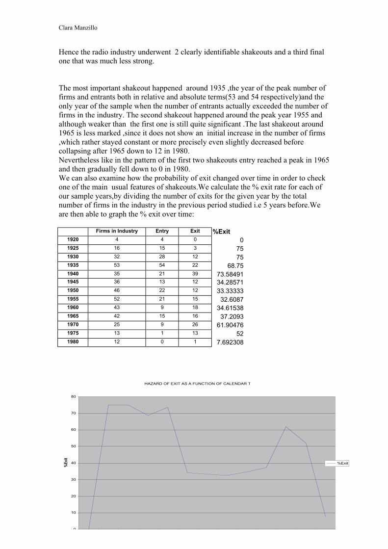
The most important shakeout happened around 1935 ,the year of the peak number offirms and entrants both in relative and absolute terms(53 and 54 respectively)and theonly year of the sample when the number of entrants actually exceeded the number offirms in the industry. The second shakeout happened around the peak year 1955 andalthough weaker than the first one is still quite significant .The last shakeout around1965 is less marked ,since it does not show an initial increase in the number of firms,which rather stayed constant or more precisely even slightly decreased beforecollapsing after 1965 down to 12 in 1980.Nevertheless like in the pattern of the first two shakeouts entry reached a peak in 1965and then gradually fell down to 0 in 1980.We can also examine how the probability of exit changed over time in order to checkone of the main usual features of shakeouts.We calculate the % exit rate for each ofour sample years,by dividing the number of exits for the given year by the totalnumber of firms in the industry in the previous period studied i.e 5 years before.Weare then able to graph the % exit over time:

Firms in Industry Entry Exit %Exit1920 4 4 0 01925 16 15 3 751930 32 28 12 751935 53 54 22 68.751940 35 21 39 73.584911945 36 13 12 34.285711950 46 22 12 33.333331955 52 21 15 32.60871960 43 9 18 34.615381965 42 15 16 37.20931970 25 9 26 61.904761975 13 1 13 521980 12 0 1 7.692308

HAZARD OF EXIT AS A FUNCTION OF CALENDAR T

0

10

20

30

40

50

60

70

80

%Ex

it

%Exit

Clara Manzillo

6

We do not observe a rise in the % exit rate during the time of the first two shakeoutsbut rather a stable % exit rate ( it is increasing during the third shakeout).This fact isconsistent with the findings of shakeout empirical analysis.We can infer the cause ofthe shakeouts is not a rise in the chance of exit since the hazard of exit remainsconstant but rather a radical fall in the level of entry:as the number of entrants falls,itbecomes inferior to the number of exiting firms and as a result the number of firmsstarts declining.Additionally ,if we graph the number of producers versus unit sales over time,we canconclude the first two shakeouts in the radio industry are not caused by Demand forthe product drying up:

Yearsavailable

Numberof firms

Entry Exit Sales

1920 4 4 0 -1925 16 15 3 -1930 32 28 12 27701933 - - - 72821934 - - - 98761935 53 54 22 104631937 - - - 113251940 35 21 39 -1945 36 13 12 -1948 - - - 156551950 46 22 12 -1951 - - - 143821954 - - - 121521955 52 21 15 -1958 - - - 114181960 43 9 18 -1963 - - - 198101965 42 15 16 -1968 - - - 115561970 25 9 26 -1975 13 1 13 -1980 12 0 1 -

Evolution of number of firms versus total unit sales

0

10

20

30

40

50

60

1920 1925 1930 1933 1934 1935 1937 1940 1945 1948 1950 1951 1954 1955 1958 1960 1963 1965 1968 1970 1975 1980

Year

Num

ber o

f firm

s

0

5000

10000

15000

20000

25000

Tota

l uni

t sal

es (m

illio

ns)

Firms at Risk

Sales

Clara Manzillo

7

As a matter of fact during the first two shakeouts in the radio industry,although thenumber of firms fell substantially, sales kept paradoxically rising at an increasingrate:from 1935 to 1948 sales increased from 10463 units to 15665 units. And from1958 to 1963 they increased from 11418 to 19810.On the contrary during the period of third more obscure shakeout, sales decreasedsharply from 19810 units in 1963 to 11556 units in 1968.This suggests that the thirdshakeout was indeed due to a fall in Demand for radio sets.Since sales dropped only in the case of the third skakeout ,there must obviously existother reasons than a fall in demand that account for the first two shakeouts.If we graph the number of radio receiver patents issued over time,we can observe adefinite rise in the number of patents over the period of the first shakeout(around1935) and a second less pronounced rise at the time preceding the secondshakeout(around 1950):

So we may conclude that each of these shakeouts was caused by some importanttechnological change regarding radio receivers.Actually, if we refer to the technological development of radio we can identify thefirst shakeout with the replacement of crystal sets by valve receivers in the early1930’s ,and the second one with the replacement of valves by transistors in the late1940’s.As for the third shakeout, it could also be explained by some particularinnovations:the development of stereophonic sound(1958) and of VHF-transmissionand frequency modulation (1955).Consequently one could argue that these revolutionary technological innovations thatpreceded the shakeouts stimulated Demand for radio sets(the new sets were of a betterquality) which in turn led to a rapid increase in the number of entrants ,willing to takeadvantage of the benefits of the new technology on the market for radio sets. We canmake the hypothesis that these “late” entrants were subsequently eliminated by themore skilled early entrants.

Receiver Patents In Specific Years

0

10

20

30

40

50

60

1920

1923

1926

1929

1932

1935

1938

1941

1944

1947

1950

1953

1956

1959

1962

1965

1968

1971

1974

1977

1980

Nu

mb

er

of

pate

nts

Clara Manzillo

8

Thus we are given the impression that technological factors seem to have been thesource of the first two shakeouts in the radio industry and hence are crucial inexplaining the survival of firms over time. The third shakeout was more presumablybrought about by the standardisation of radio sets and their maximum level ofperformance reached,leading to a saturation of the market:after the establishment ofthe solid state equipment(transistors), there was little scope for further basicimprovement and as a result the incentive to buy a new radio set was clearly reduced(radios generally lasted very long).In fact after 1960, the number of radio receiverpatents issued became nearly negligible and hence presumably crucial productinnovations ceased .One can therefore speculate that by 1960 radio sets had reached a“dominant design”(Utterback and Suarez,1993,p.1-21)i.e could not be made obsoleteanymore .Other reasons for the fall in demand for radio sets have been offered suchas “recession ,foreign competition and Government tax policy”(The United Kingdommarket for domestic audio and TV equipment,1997,p.iii) and obviously the increasingsuccess of television.At this point in order to explain better the pattern of shakeouts in the radio industry,itmay be useful to turn to some formal theories of shakeouts.Many models have been developed on the causes and consequences of shakeoutsespecially since shakeouts have been identified as one of the major sources ofconcentration i.e the establishment of oligopolies , especially if the remaining firmsare the early entrants because they had time to grow gradually over time.Infact the natural result of the sequence of shakeouts the radio industry appears tohave experienced was a permanent reduction in the number of competing firms (froma peak level of 53 in 1935 down to only 12 in 1980)i.e a high level of concentrationin the industry.In effect, nowadays there are only 3 radio receivers manufacturerslisted in the 2001 Kelly’s Directory:AMS neve PLC, Bush Radio Plc and MarineElectronic Suppliers.These are huge companies producing a range of electronicsproducts.The United States radio industry appears to have been characterized by asimilar shakeout process and is also quite concentrated.Hence oligopoly in the radioindustry is probably a natural market stucture which cannot possibly be avoided andresults from the basic nature of the industryWe will now concentrate on a particular theory of shakeout developed by Klepperand Simons (1993,1997) and check if the empirical results obtained from our datasetmatch with the elements of this model. First let us discuss the main features of thismodel:This model assumes firms enter fairly small,but then grow gradually . First manyfirms are attacted by the new market and are able to enter because prices are still quitehigh and even relatively incompetent firms can achieve positive profits.Over time thenumber of producers increases and existing firms expand so if the Demand functionremains the same,the price(hedonic and inflation adjusted ) falls.Then, as expectedprofits keep going down , only the most competent i.e a smaller and smallerproportion of the potential entrants decide to enter.As a result,the level of entrydecreases until it reaches zero when no firm can enter profitably anymore.As exitcontinues normally and entry falls,the number of producers in the industry declinessubstantially. According to this model , early entrants have a significant advantageover later entrants in the industry and survive better in the long term because of theirlarger size and geater expertise.

Clara Manzillo

9

This model argues that early entrants enter when the price of the product is still highand there is the opportunity to earn very high profits and then grow and gainexperience over time so that they become the larger most skilled firms in theindustry(since the growth rate is limited in practice as marginal costs of growth areincreasing).Since both size and skills drive costs down and increase efficiency,theearly entrants are generally more profitable firms and tend to survive longer anddominate the industry through reinforcing technnology,wiping out the late smallerless skilled competing firms which are not able to keep making positive profits asprices fall.So the positive role of early entry ,size and skills on survival are underlinedin this model .Some of the assumptions of this model are the following:_Firms enter small.Although in the radio industry “standardization of parts and relatively little use ofhighly trained workers have also enabled many assemblers to enter the industry withsmall amounts of capital”(,1952,p.1),which makes this assumption valid,there mighthave been some heterogeneity in entrants’sizes(some new entrants may have beenlarge firms specialised in other products or based overseas).Yet it could still be said ifwe assume firms grow gradually over time that on the whole,early entrants are largerthan later ones at any point in time._The demand function is stable.This is a questionable assumption in the radio industry since the level of demandmight have shifted over time, up when new innovations were introduced andimproved considerably the quality of radio sets making them more attractive toconsumers , or down when television was introduced and radios were not perfectedanymore._Technology in the industry is essentially of the sustaining type(processinnovation,improvements in production methods) thus reinforces the leadership ofearly entrants which can rely on their past relevant experience. It could be argued that this may not exactly the case in the radio industry where,although gradual continuous innovations were frequent and contributed to thesuccess of some firms, a number of dramatic technological changes considerablytransformed the initial product.So these assumptions seem slightly problematic in the context of the radio industry.However the model may still accurately depict the evolutionary dynamics of thisindustry.In order to check whether the Keppler&Simons model applies to the radio industry,we will now test its hypothesis more formally .We also aim at evaluating the effect ofa number of characteristics of firms on their survival, we will use the techniques ofsurvival analysis applied to our data sample.Our data set lists all the companies in the industry fom 1920 to 1980 .It contains 203observations and each line has 7 variables i.e for each firm 7 corresponding variablesare given :1. “entryyr”:its respective year of entry i.e the approximate date at which it began

producing radio sets .Since we started collecting data from the year of thebeginning of the industry,we can assume that all producers are 0 years old i.e haveproduced the product for 0 years , when they are first listed in the register.So nofirm could have existed before 1920,the first year in our sample.Hence there in noproblem of left-sample truncation.

2. “exityr”:its year of exit (or 1985 ,if it still appears in 1980:right censoring) i.e itsapproximate last year of production.

Clara Manzillo

10

3. Its “totalage” i.e the approximate number of years it remained in the industry.Wecalculated totalage as the difference between year of exit and year of entry sincewe collected data at a 5 year interval and we assumed that in practical terms theaverage company entered the industry 2.5 years before the year we found it firstlisted (i.e the theoretical ‘ year of entry’) and exited 2.5 years before the first yearwe do not find it listed anymore(i.e the theoretical ‘year of exit’).When we found gaps in our data collection ,we assumed that the firms remainedproducers during the apparent gaps.

We have added 3 dummy variables that could have an effect on survival:4. “London”:this variable takes the value 1 if the firm is based in London,a 0 otherwise and is formed using the company’s location.5. “Ltd.”:this variable equals 1 if the firm is a Limited company,a 0 otherwise and is

simply directly inferred from the company’s name.This variable should give ussome rough idea of the firms’sizes since we would expect the group of limitedfirms to correspond to larger firms.

6. “TV prod”.:this variable is given the value 1 if the firm also entered the TVindustry ,a 0 otherwise and was derived by indentifying the radio sets firms in thelist of all UK manufacturers of TV sets registered in the Kelly’s Directory .Radiosets firms containing the word television in their name were also considered as TVproducers.

Finally we tried to assess somehow the impact of technology on survival in the radioindustry by studying the effect of the following variable:7. “ patents”:average number of radio patents per year received by each firm.The overall number of radio patents for each firm was determined by carrying out apatent search at the patent database at “http:gb.espacenet.com”:we entered the firm’sname under the category “Applicant” and the word “radio” under “title”.This patentsearch is not quite a detailed one since we only looked for patents of firms which havesurvived at least 10 years(totalage>=10) and for patents containing the word radio intheir title,which might have only yielded partial results. Moreover we have notestimated the relative values of the patents delivered. However we have accounted forthe firms’distinct totalages: the approximate ( average) annual number of radiopatents granted to each company was worked out by dividing the total number ofpatents found for each firm by its totalage.The resulting value should provide a crudemeasure of the firm’s technological activity or level of R&D undertaken in thespecific radio field(some firms also issued other types of electronics patents but wedid not include them in the total number of patents although these firms may havealso benefited from these broader type of technology).A summary of the data is given below,with the usual measures of centraltendency(mean,min,max),and dispersion in the data(standard deviation, maximumrange):

Variable Obs Mean Std. Dev. Min Max

entryyr 203 1943.424 13.52401 1920 1975exityr 203 1953.596 16.26283 1925 1985London 202 .5 .5012422 0 1Ltd 203 .7241379 .4480526 0 1totalage 203 10.17241 10.3333 5 65

TVprod 203 .1871921 .39103 0 1 Patents 73 2.891808 18.31023 0 155

Clara Manzillo

11

We make the following assumptions to analyse our data:_As mentioned before,we consider that the firms with entryyear equal to 1920,the firstyear of our sample,did not produce radios in earlier years.This is reasonable sincethere is no section on radio receiving sets manufacturers in the Kelly’s Directoriesbefore 1920.However these firms may have actually been present before 1920 aswell-established manufacturers of other products but this does not represent a problembecause exit and survival in our analysis are not defined in terms of existence but interms of production of radio sets: a firm is said to exit when it ceases to produce radiosets pesumably because it is not competitive any more and makes negative profits._Given that we do not possess any information on acquisitions and mergers,weassimilate an acquisition or a merger as an exit of one of the firms and the survival ofthe other(the firm whose name has been kept , assuming that the firm formed isnamed after one of the two original producers).First of all,we check for early-mover advantage by interpreting two-by-two tables ofsurvival length versus time of entry.We can infer from these tables whether earlierentrants had better chances of surviving a particular number of years.This methodinvolves the choice of an arbitrary dividing date separating early entrants from laterones and a precise duration of time for the survival age.We selected the year 1930 asthe critical year between the early entry cohort and the late entry one:we generateearly1=entryyr<1930 i.e we define early entrants as firms which began productionbefore 1930 i.e either in 1920 or 1925 as we consider the period 1920-1930 or moreprecisely 1917.5-1927.5 to be the early stage of the industry when the number ofproducers was still relatively low.To begin with ,we study survival over at least 10 years,exluding firms which enteredafter 1975i.e in 1980(we generate tenyear>=10 and usedata=entryyr<=1975) since itis impossible to determine from our data whether their totalage is at least 10 years.Weobtain the following results:

early1 0 1 Total

0 117 67 18463.59 36.41 100.00

1 15 4 1978.95 21.05 100.00

Total 132 71 20365.02 34.98 100.00

Fisher's exact = 0.2151-sidedFisher's exact = 0.138

We find how many firms belong to each category and the correspondingpercentages,given below these numbers.So the late entrants correspond to 184firms,67/184≈36.41 % of which survived at least ten years(67 firms) whereas only4/19≈21.05% of the early entrants(4 over 9 firms) have a totalage equal or greater to10.

Clara Manzillo

12

These figures seem to indicate that later entrants performed better in terms of 10-yearssurvival.The “p value” fom Fisher’exact test is equal to 0.215.This number impliesthat if the 2 categories of cohorts(early and late entrants) had exactly identical chancesof surviving to age 10 then the probability of finding such a large difference betweensurvival rates in each category(36.41-21.05=15.36) just as a result of randomvariation would be 21.5%,which is a rather small chance.Hence this apparentdisadvantage of early entrants versus late ones cannot simply be attributed to somerandom events.

Now let us consider twenty years as the survival length(we generate twenyear>=20and usedata entryyr<=1965):

twenyearearly1 0 1 Total

0 150 24 17486.21 13.79 100.00

1 17 2 1989.47 10.53 100.00

Total 167 26 19386.53 13.47 100.00

Fisher's exact = 1.0001-sidedFisher's exact = 0.512

The fraction of late entrants surviving at least 20 years(13.79%)is very close to thefaction of early entrants surviving at least 20 years (10.53%).As a result the Fisher’sexact is approximately 100%:survival rates will almost always be at least as far apartas 10.53% and 13.79% even if early and late entrants have the same chances ofsurviving 20 years.Similarly for 30 years survival,the percentages for early versus late entrants are nearlyequal(9.40 % and 10.53% respectively):

thiryearearly1 0 1 Total

0 135 14 14990.60 9.40 100.00

1 17 2 1989.47 10.53 100.00

Total 152 16 16890.48 9.52 100.00

Fisher's exact = 1.0001-sidedFisher's exact = 0.565

Clara Manzillo

13

For 40 years survival,the results lead to different conclusions:

fortyearearly1 0 1 Total

0 98 7 10593.33 6.67 100.00

1 17 2 1989.47 10.53 100.00

Total 115 9 12492.74 7.26 100.00

Fisher's exact = 0.6271-sidedFisher's exact = 0.415

6.67% of late entrants managed to survive this long versus 10.53% of early entrantsbut the value of the Fisher’exact is 62.7%i.e it is larger than 50% so the results are notvery meaningfull statistically and one should not draw conclusions from these resultsin terms of relative chances of exit for early entrants versus late ones.Similarly in terms of 50 years survival,early entrants performed better than late ones:

fiftyearearly1 0 1 Total

0 71 2 73 97.26 2.74 100.00

1 17 2 19 89.47 10.53 100.00

Total 88 4 92 95.65 4.35 100.00

Fisher’s exact = 0.1881-sidedFisher’s exact = 0.188

However in this case,not only is the difference between the percentage of early andlate entrants having survived wider(2.74% for late entrants versus 10.53%for earlyentrants)but the Fisher’exact equals only 18.8%,making these results more valid interms of relative probability of exit of the two entry cohorts.So at old totalages,thesurvival rates are high for early entrants and low for late ones .We can also use a different approach to compare survival chances between the earlyand later entrants groups.We can plot Kaplan-Meier survival curves for the twogroups and make comparisons.This is a more general method,which does not requirethe choice of an arbitrary dividing date for survival age and entry time.

Clara Manzillo

14

The category survival time in the table below shows the totalage by which 25%,50%and 75% of firms had exited:

incidence no. of -- Survival time -----early1 timeat risk rate subjects 25% 50% 75%

0 1855 .0932615 184 5 5 101 210 .0857143 19 5 5 5

total 2065 .0924939 203 5 5 10

Both survival curves are constructed by plotting the percentage of firms in the datathat survived a given amount of time according to whether these firms are earlyentrants or not:

This graph gives the impression , as we found previously ,that early entry gave anadvantage for survival not in the short run but in the long-run since the two curvesintersect,the curve corresponding to early entrants going above the late entrants curveafter a survival age of about 25 years(it is clearly above only starting from a totalageof 30 years).So both the two-by-two tables and the Kaplan-Meier survival curves suggest thepossibility of an advantage of early entrants for survival chances but only over a verylong time period(more than about 30 years of participation in the industry).It can be argued that this complete absence of competitive advantage of early entrantsin the short and medium term i.e at relatively early totalages is consistent with theprevious finding of a constant percentage exit over the time of the two first shakeoutsin the radio industry:we may suggest that whenever the percentage exit ( ratio of exitsto the number of firms in the previous period) remains the same throughout theshakeout period then survival over that period has no tie in with any supremacy of oldentry firms.

Kaplan-Meier survival estimates, by early1

analysis time0 20 40 60 80

0.00

0.25

0.50

0.75

1.00

early1 0

early1 1

Clara Manzillo

15

In fact,if that ratio stays constant while at the same time the level of entry first goes upand then comes down,it may be surmised that the propensity,as to say,to exit is thesame for “old”,incumbent firms as for “new” firms,otherwise the average propensitywould vary along with the level of entry(unless of course ,for the sake of theargument,one would imagine a complicated relationship where the two singlepropensities would vary according to the relative presence of the old and new entrantsso as to keep the average equal).This is equivalent to saying that the differencebetween “old” and “new” is not a significant variable for survival over the shakeoutand the entire process correlates with exogenous factors.An analogy may be given bya chemical reaction where the ratio between the product(exit) and the reactants inplace varies only with the physical factors(temperatures,pressure etc…)because ofcourse molecules are all the same.Moreover the absence of early entry advantage found at relatively small totalagesdoes not contradict the Keppler&Simons model since “the heterogeneity in potentialentrants’capabilities” and the increased competence required to enter the industry inlater stages can explain why survival rates do not differ between early and laterentrants initially: in the early years of the industry,numerous incompetent firms mighthave stepped into the industry but as possible profits become very low in the latestages and if diffusion of technology is widespread and access to it not too difficultlate entrants happen to be more skilled and knowledgeable than incumbent firms sothat this superior competence of later entrants outweighs the advantage of earlyentrants related to size and as a result both types of firms will then have equal chancesof exit since both size and competence play a role for survival.So the opposing effectsof early entry and increased competence accompanying late entry tend to cancel eachother out so that the probability of exit becomes independent of the time ofentry(same percentage exit for early and late entrants).Consequently the Keppler&Simons theory of shakeouts appears to fit well theevidence in the case of the radio industry.However this theory primarily relies on a definite advantage of early entrants drivinglater entrants out of the market and contrastedly the theory of early mover advantagedoes not hold at all for small and medium totalages.Although this surprising resultcould be explained by some assumptions of the Keppler&Simons model,we wouldexpect a apparent advantage of early entrants at younger totalages than 30 years.It may be noted that in the very much reduced number of radio firms present in themarket in 1980,all have entered the industry before or in 1950 ,whereas if earlyentrants had the same chances of survival than later entrants,we would have expecteda very large proportion of later entrants among the censored firms(later entrants havemore chances of surviving until 1980 ceteris paribus given that their totalage is lowerfor any exityear).Therefore in order to clarify the role of early entry in the radio industry and maybefind a stronger advantage of early entrants,we should perhaps take into account thedisruptive side of the radio technology and redefine the concept of early entry in termsof relative early entry at the beginning of each shakeout when a radical innovation hasjust taken place and profitability is maximum , or more simply change the criticalyear between early entrants and late entrants from 1930 to 1955(i.e generate early 2=entyyr<1950)so as to include both early entrants at the time ofthe first shakeout and at the time of the second shakeout.Then the results obtained do highlight an early mover advantage at younger totalages:

Clara Manzillo

16

twenyearearly2 0 1 Total

0 43 4 4791.49 8.51 100.00

1 124 22 14684.93 15.07 100.00

Total 167 26 19386.53 13.47 100.00

Fisher's exact = 0.3301-sidedFisher's exact = 0.186

15.07% of early entrants(by 1950)versus only 8.51% of late entrants have survived 20years and the value of Fisher’s exact(33%) is acceptable.For the older totalage ,30 years,the advantage of early entrants appears as verymarked:

.thiryear

early2 0 1 Total

0 22 0 22100.00 0.00 100.00

1 130 16 14689.04 10.96 100.00

Total 152 16 16890.48 9.52 100.00

Fisher's exact = 0.134 1-sided Fisher's exact = 0.094

10.96% of early entrants have survived 30 years versus 0% of late entrants and theFisher’exact is quite low:13.4%.The new criteria for early entry yields far better results than before for the advantagerelated to early entry.So apparently it is not so much the very early entrants whichhave an advantage but rather the early entrants at the beginning of each shakeout.Now let us verify the effect of some other firms’traits over their survival._Firstly to assess the role of size ,we use the proxi Ltd.Again we use 2-by-2 tables inorder to compare firms’survival over at least 10 years depending on whether theywere Limited companies:

Clara Manzillo

17

tenyearLtd 0 1 Total

0 45 11 5680.36 19.64 100.00

1 87 60 14759.18 40.82 100.00

Total 132 71 20365.02 34.98 100.00

Fisher's exact = 0.0051-sidedFisher's exact = 0.003

So the percentage of Ltd.firms which have survived at least 10 years is 40.82%compared to only 19.64% for non Ltd.firms.Fisher’s exact test(0.5%) indicates thatthe results are reliable for general deductions about the role of Ltd.i.e size onsurvival:there is only a 0.5% chance to find such a disparity between survival ratesjust due to random factors.This advantage of Ltd.firms can be confirmed by plottingthe proportion of firms surviving to each age for Ltd.firms versus non Ltd.ones:

These Kaplan-Meier survival curves seem to indicate clearly far better survival ratesfor Ltd.firms : the Ltd.curve is markedly above the non Ltd.one and the log rank andWilcoxon(Breslow) test for equality of survivor functions give a low probability(respectively 1.25 % and 0.64%)of this difference in the curve happening just byrandom chance if Ltd. and non Ltd. Firms had exactly the same chances of survival atdifferent ages.Thus Ltd.firms survive seemingly much better.We might infer that size and survivalare tightly positively related .This result fits the Keppler&Simons hypothesis thatlarger firms perform better because they spread costs of R&D over more output andhence spend more on R&D,which leads to lower costs and a better product qualitythan smaller firms.Alternative reasons have been offered for the advantage enjoyed by

Kaplan-Meier survival estimates, by Ltd

analysis time0 20 40 60 80

0.00

0.25

0.50

0.75

1.00

Ltd 0

Ltd 1

Clara Manzillo

18

large firms:easier access to financial means,higher efficiency,economies of scale inproduction or methods(minimum efficient scale)or advertising cost spreading._Now let us examine the effect of the firms’location on their survival by using aKaplan-Meier survival plot:

So we find that the firms based in London tend to survive better.This is probably dueto the benefits from agglomerative networks&cities on the success of companies;firmsin London dispose of a pool of information,suppliers,skilled personnel,contracts andfinancial means and of easier means of transport and infrastucture._The final dummy variable to analyse is TV prod.A study by Keppler&Simons (2000)found that survival in the TV industry was significantly better for firms which wereprevious radio producers since radio experience prooved very useful for TVmanufacturing .We would like to determine if the converse is also true i.e if enteringthe TV industry caused a rise in radio firms’chances of survival. So we can graphKaplan-Meier survival curves for radio firms manufacturing TVs and for radio firmswhich have not entered the TV market:

Kaplan-Meier survival estimates, by London

analysis time0 20 40 60 80

0.00

0.25

0.50

0.75

1.00

London 0

London 1

Kaplan-Meier survival estimates, by TVprod

analysis time0 20 40 60 80

0.00

0.25

0.50

0.75

1.00

TVprod 0

TVprod 1

Clara Manzillo

19

At first sight,ther appears to be a clear advantage of firms which have entered the TVindustry(the TV prod.curve is well above the non TV prod. curve).However television manufacturing started only around 1950 so including the firmswhose entryyear is less than 1950 may be misleading:it introduces a bias in favour ofan advantage of radio firms(all the firms which died before 1950 are considered asnon TVprod,thus probably incresing the apparent hazard of exit of non TVprod).Therefore it would be more rigorous to consider only firms whose entryyear isgreater than 1950.We can tabulate the variable TVprod versus ten years survival forfirms wose entryyear is strictly between 1950 and 1975(usedata=1950<entryyr<1975)since we also exclude firms having entered in 1980(we ignore whether they survived10 years):

tenyearTVprod 0 1 Total

0 116 49 16570.30 29.70 100.00

1 16 22 3842.11 57.89 100.00

Total 132 71 20365.02 34.98 100.00

Fisher's exact =0.002 1-sided Fisher's exact =0.001

These tables show that among radio firms, 57.89% of TV producers survived 10 yearsversus only 29.70% of non TV producers.Moreover the value of Fisher’exact islow:0.2%.Since this analysis is more precise and provides more trustworthy conclusions wemay suggest that as a general rule radio firms benefited from entering the TVindustry.The explanation might be that the usual success radio firms had in the TVindustry,due to their know how enabled those firms to increase substantially theirsize,which has been identified as a plausible effective factor influencing survival .At this point,in order to model the effect of the 3 dummy variables analysedpreviously on the hazard of exit,we suppose that these factors affect firms accordingto the following exponential hazard model:

By carrying out an exponential regression,we can determine the “maximum-likelihood estimates” of the constant terms β1, β2, β3 and α :

Clara Manzillo

20

Exponential regression -- log relative-hazard form

No. of subjects = 202 Number of obs = 202No. of failures = 190Time at risk = 2060

LR chi2(3) = 27.93Log likelihood = -259.75651 Prob > chi2 = 0.0000

_t Coef. Std. Err. z P>z [95% Conf. Interval]

London -.1044826 .1461688 -0.715 0.475 -.3909683 .182003Ltd -.3142489 .1618375 -1.942 0.052 -.6314446 .0029468TVprod -.8021588 .1972402 -4.067 0.000 -1.188743 -.415575_cons -1.900418 .1541794 -12.326 0.000 -2.202604 -1.598232

The “maximum-likelihood estimates” are given in the column “Coef.”so:α(“cons.”)= -1.900418β1(“Ltd.”)= -0.3142489β2(“London”)= -0.1044826β3(“TV prod”)= -0.8021588Therefore the estimated model is :

=exp(-1.90048-0.3142489Ltd.-0.1044826 London –0.8021588 Tvprod.)

The estimated hazard of firms which were not Limited nor in London nor TVproducers is equal to exp(-1.90048)=0.149496844 per unit of time i.e approximately15% per year,whereas h for firms which are Limited,based in London and TVproducers is just equal to:exp(-1.90048-0.3142489.-0.1044826 -0.8021588 )=exp(-5.4404578)=0.004337497(since Ltd=1,London=1 and TVprod=1),i.e about 0.4% per year,which is almostfourty times smaller than for non Ltd.radio firms in Provinces not producing TVs.Indeed,the values of β1,β2, and β3 are all negative numbers so that the variablesLtd.,London and TVprod.all appear to have a negative effect on the hazard of exit,i.ethose characteristics of companies reduce the probability of exit as shown previouslythrough survival curves.However the 95% Confidence Intervals for the coefficients ofthe variables London and Ltd contain zero,so at the 95% confidence level,we acceptthe null hypothesis that the real coefficients equal zero,i.e that the variables Londonand Ltd. are statistically insignificant.Yet the “p values”(found in the column P>z)indicate that if the true values for β1and β2 were equal to zero then there would beless than a 50 %(47.5% for β1,only 5.2% for β2) chance to find such large values ofβ1and β2.As for the variable TVprod.,it is significant(zero does not belong to the 95%confidence interval) and if β3 was equal to zero then there would be less than0.1%chance to find such a large β3,but these results are likely to be biased given thatTV production started only around 1950.We can also use the Cox model to represent the effects of the variables Ltd.,Londonand TVprod.:

Clara Manzillo

21

Given that in our case all firms did not enter at the same point in time,age isequivalent to time since the first year in our sample,1920.So f(age)=f(t).As we wouldalso like to assess the effect of totalage on the hazard of exit,we can add the variabletotalage:

By running a Cox regression,we find:

Cox regression -- Breslow method for ties

No. of subjects = 202 Number of obs = 202No. of failures = 190Time at risk = 2060

LR chi2(4) = 234.54Log likelihood = -798.66533 Prob > chi2 = 0.0000

_t_d Coef. Std. Err. z P>z [95% Conf. Interval]

Ltd -.0181459 .1651291 -0.110 0.912 -.3417929 .3055012 London -.0211275 .1469626 -0.144 0.886 -.3091688 .2669139

TVprod .0107168 .2026144 0.053 0.958 -.3864002 .4078338totalage -1.398466 .1454856 -9.612 0.000 -1.683613 -1.11332

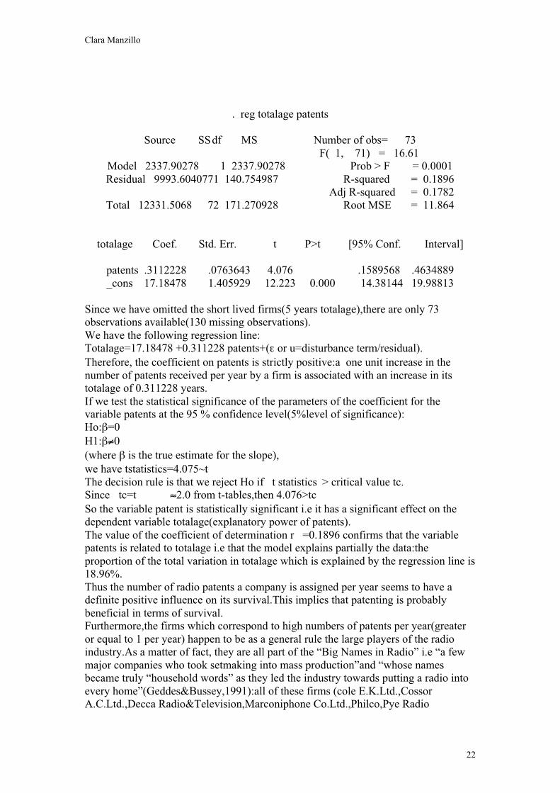
This model gives different result for the coefficients of the dummy variables and inparticular a positive coefficient for TVprod.The “maximum partial likelihood estimate” for the factor totalage isβ4= –1.398466<0 , the absolute value of z is high(9.612) and the “p value” is lessthan 0.1% ( totalage is a very significant variable) .Hence totalage seems to have astrong positive effect on survival.The hazard of exit appears to depend on thefirms’totalage and to be smaller at old totalages i.e when firms have been in themarket already for a number of years.Old firms have probably lower chances of exitbecause they have been able to grow and gain experience over time so they may beahead of younger firms in terms of size and skills.Finally let us evaluate the role of patents on survival.We have already shown therelevance of patents during shakeouts but the effect of patents on performance has notbeen qualified yet.There is a wide diversity in the number of patents corresponding to firms whosetotalages are equal.Some long lasting firms did not have any patent related to radiolisted under their names whereas other firms received a high number of patents peryear containing the word radio in the title(for example 155 for the MarconiphoneCo.Ltd. and 22.45 for Bosch Ltd ).Hence at first sight,one may have the impressionthat patents are not essential for success in radio manufacturing or that most of thepatents received are of relative unimportance and easy to design around or perhapsthat licensing is frequent and more crucial than patenting itself.However, if we regress totalage on patents,totalage being the independent variableand patents the explanatory variable, we obtain the following results:

Clara Manzillo

22

. reg totalage patents

Source SSdf MS Number of obs= 73 F( 1, 71) = 16.61

Model 2337.90278 1 2337.90278 Prob > F = 0.0001Residual 9993.6040771 140.754987 R-squared = 0.1896

Adj R-squared = 0.1782Total 12331.5068 72 171.270928 Root MSE = 11.864

totalage Coef. Std. Err. t P>t [95% Conf. Interval]

patents .3112228 .0763643 4.076 .1589568 .4634889_cons 17.18478 1.405929 12.223 0.000 14.38144 19.98813

Since we have omitted the short lived firms(5 years totalage),there are only 73observations available(130 missing observations).We have the following regression line:Totalage=17.18478 +0.311228 patents+(ε or u=disturbance term/residual).Therefore, the coefficient on patents is strictly positive:a one unit increase in thenumber of patents received per year by a firm is associated with an increase in itstotalage of 0.311228 years.If we test the statistical significance of the parameters of the coefficient for thevariable patents at the 95 % confidence level(5%level of significance):Ho:β=0H1:β≠0(where β is the true estimate for the slope),we have tstatistics=4.075~tThe decision rule is that we reject Ho if t statistics > critical value tc.Since tc=t ≈2.0 from t-tables,then 4.076>tcSo the variable patent is statistically significant i.e it has a significant effect on thedependent variable totalage(explanatory power of patents).The value of the coefficient of determination r =0.1896 confirms that the variablepatents is related to totalage i.e that the model explains partially the data:theproportion of the total variation in totalage which is explained by the regression line is18.96%.Thus the number of radio patents a company is assigned per year seems to have adefinite positive influence on its survival.This implies that patenting is probablybeneficial in terms of survival.Furthermore,the firms which correspond to high numbers of patents per year(greateror equal to 1 per year) happen to be as a general rule the large players of the radioindustry.As a matter of fact, they are all part of the “Big Names in Radio” i.e “a fewmajor companies who took setmaking into mass production”and “whose namesbecame truly “household words” as they led the industry towards putting a radio intoevery home”(Geddes&Bussey,1991):all of these firms (cole E.K.Ltd.,CossorA.C.Ltd.,Decca Radio&Television,Marconiphone Co.Ltd.,Philco,Pye Radio

Clara Manzillo

23

Ltd.)except the Burndept Ltd. And Bosch Ltd. ,are cited in the chapter “the big Namesin Radio” and are identified as the major producers in the radio setmaking industry.Consequently the other radio long lasting firms have probably survived by buyinglicenses from the large main companies.So we may conclude that the amount of patenting,which is probably a good indicatorof the level of research undertaken is one of the major determinants of thefirms’success regarding both expansion and survival.This suggests that patents in theradio industry give high benefits in practice,are well-enforced(difficult to get around)and/or represent a very operative protective barrier against competing firms andpotential entrants.

Before drawing any conclusions fom our data analysis,we must not disregard thelimitations of this analysis._Since our data was collected at a 5 years interval,it is discontinuous i.e it containsgaps so we have certainly omitted some short–lived firms in the industry.Moreoverfirms were not compelled to register on the directories and the smallest firms may nothave been listed._We have no information on mergers and acquisitions so we might have consideredsome renamed merged firms as new entrants and some merging firms as exitingcompanies._As a whole radio sets firms were not specialized in manufacturing radio sets.Mostproduced other electronics products such as radio components and “ other soundreproduction equipment,television sets or record&tapes”(IPC Marketingservices,1997,p.7).These other specific product industries undoubtedly affected thesurvival of radio sets firms.Thus the analysis for the individual industry segment ofradio sets is not pure i.e it was most probably contaminated by the respectiveevolutions of those parallel industries and the role played by our variables in thoseindustries.Therefore ideally we would consider only radio sets firms producingexclusively radio sets but such firms would be very difficult to find and anyway thestudy would not be representative anymore._Finally one serious problem in terms of interpretation is that even if we find bysurvival or regression analysis a variable to be significantly associated with a highersurvival,we have no way to ascertain the direction of causation or even establish theexistence of a cause-effect type of relationship.Indeed the variables could beinterdependent (endogeneity bias) or worse both directy influenced by some otherexternal variable responsible of the real effect on survival(spurious correlation).So we cannot directly deduce from our analysis that large and patent holding firmssurvive better.A clarification of the causal relationship would require a finer statisticalanalysis of time series data tying individual firms previous size or number of patentsto their subsequent success.A publication such as for example “The Setmakers,ahistory of the radio and telavision industry”by Geddes,K. & G.Bussey could assist usin undertaking this more detailed study.Probably the definition of the meaningfullparameters to be measured for success would be the most difficult task.Although , as we have pointed out ,our analysis is rather appoximate, we can stilldiscuss some possible conclusions regarding the patterns of exit and survival in theradio industry and their consistency with the theory expressed by Klepper&Simons.

Clara Manzillo

24

In the model of Klepper&Simons ,it is assumed that the pattern of shakeouts is due tothe advantage of skilled early entrants in the case of reinforcing technology.A classical example offered is the automobile industry where a unique shakeoutbrought about the present oligopoly. On the contrary the radio industry is an exampleof a combination of continuous sustaining technology and disruptivetechnology,where rather than a unique shakeout,a sequence of multiple shakeouts didoccur.We have tried to show that this multiplicity might be associated with disruptiveinnovations, whereas each shakeout taken separately is probably a result of sustainingtechnology.Since we do not find any early mover advantage in the industry,we canmake the following hypothesis:the very early entrants ,or more precisely in eachshakeout period the early entrants of the previous stage did not necessarily adopt thefundamental revolutionary innovations which marked the development of radio sets.In effect each innovation gave rise to a totally new product that was not producedusing the same methods as before ,so that earlier firms already present in the industryat the beginning of the shakeout did not have necessarily an advantage,or evenperhaps had a disadvantage versus entrants just entering at the beginning of theshakeout process i.e when the innovation had just taken place and profitability was atits highest level.Hence this technological explanation of shakeouts may relate moreto turnover of corporate leadership (blindness of early entrants)rather than earlymover advantage emphasized in the Klepper&Simons model.However if we isolate each cycle of shakeout from the others,then theKlepper&Simons model appears to be validated : in each particular cycle ,the earlyentrants seem to have had an advantage relative to later entrants in terms of survival.Moreover even though very early entrants did not appear to have a significantadvantage in terms of technology,their larger size must have been a definite assetversus later smaller competitors. In fact the 3 dummy variables London ,Ltd. andTvprod,which were found by survival analysis to have an apparent significantpositive effect on totalage, can all be associated with a large size:larger firms tend tobe Limited ,based in London and diversified.Even if these variables had an effect ontheir own on performance then still size would matter as a result since thesecharacteristics usually require a minimum size:London based companies face morecosts (rental cost ,wages…)as well as Limited companies(higher income taxes) whileentering a new industry such as the TV industry involves fairly important financialmeans( high fixed costs barriers of entry).Similarly, patenting,which was found byregression to affect positively the survival of firms is also linked with size:larger firmsgenerally patent more as patenting incurs high financing.Thus , as suggested by the Klepper&Simons model,size is very likely to play a crucialrole for survival of individual firms in the radio industry.In effect among the firms that have survived for a long time period or are still presentin the industry in 1980,most are firms that have entered either around 1925 (at thebeginning of the first shakeout period or around 1940(at the beginning of the secondshakeout period)i.e firms which were able to adopt and patent early enough the newtechnologies which caused the shakeout and as a result gained a foothold in theindustry and prevailed at least until the next shakeout ,suggesting that relative earlyentry plays a non negligible role for survival.There are only a few exceptions of lateentrants still present in 1980 and these cases are probably due to to errors in the dataor to the fact that these firms were already large at the time of entry,either specializedin other electronics areas or simply well-established overseas(such as Bosch).

Clara Manzillo

25

Thus in general,it can be argued that the long term survivors in the radio industry arelarge and diversified firms able to resist to major changes in Demand for radiosets(like the drop in demand for radio sets in the late 1960’s, fatal to numerous firms:26/42≈62% of the firms present in 1965 exited before 1975) and to lead in terms ofprocess innovations.One may wonder whether a new major radical innovationaffecting radio sets would lead to another shakeout process and more interestinglywhether these incumbent powerful firms would keep up with the innovation andmanage to remain dominant or rather be outcompeted and even forced to exit byopportunistic competent new entrants.As a final conclusion,one may suggest that both technological factors and sizedetermine in great part survival of firms in the radio industry: firms able to implementthemselves early enough to appropriate the benefits of a new fundamentaltechnological change when profitability is at its highest level and patenting is stillfeasible have the possibility to grow and establish themselves as leading firms butmay be at risk of loosing market shares or even of exiting the industry when the nextdrastic innovation occurs.Hence one might surmise that oligopolies brought about by shakeouts and maintainedthrough sustaining technological improvements are not pemanent in the radioindustry.Indeed they might be broken up by disruptive innovations which start a newcycle and so on.However it may be important to note that in the case of the radioindustry, major disruptive innovations would not really be expected since there isseemingly little scope left for further basic variations in the present solid state designof radio sets and that in addition,the last and most concentrated oligopoly wasapparently not brought about by a classical shakeout caused by technology but ratherhappened as a result of a drastic drop in demand for radios. Consequently, one maydoubt that such a concentrated oligopoly might ever be dismantled as a result of a newrevolutionary innovation.

Clara Manzillo

26

References

� Briggs,A.,1995,The History of Broadcasting in the United Kingdom :Competition:1955-1974(VolumeV) ,Oxford University Press.

� Crisell,A.,1986,Understanding Radio,Methuen.

� Geddes,K.&G.Bussey,1991,The Setmakers,a history of the Radio and Televisionindustry,The British Radio& Electric Equipment Manufacturers Association.

� Graham,W.M.,1952,Case study data on productivity and factoryperformance:Radio and Television Manufacturing,Bureau of LaborStatistics,United States Department of Labor

� Hilliard,r.l.,1985,Radio Broadcasting.An introduction to the sound medium,Longman.

� Inglis,A.F.,1990,Behind the Tube.A History of Broadcasting Technology andBusiness, Focal

� I.P.C Marketing services,1977,The United Kingdom Market for domestic audioand T.V.Equipment.

� Klepper,S.& K.L.Simons,2000, “Dominance by Birthright:Entry of prior RadioProducers and Competitive Ramifications in the U.S.Television ReceiverIndustry”,Stategic Management Journal no.10-11,vol 21(October-November),pp.997-1016.

� Simons,K.L,2001(first version 1996),Industrial Growth and Competition CourseNotes,unpublished.

� Sterling,C.& J.M Kittross,1978,Stay Tuned:A concise history of AmericanBroadcasting,Wadsworth Publishing Company Inc.

� Utterback,J.M.& F.F Suarez,1993, “Innovation,Competition,and IndustryStructure”,Research Policy no.22,pp.1-21