econometric tools for analyzing market … · recent complementary developmentsin computing power,...
TRANSCRIPT

Chapter 63
ECONOMETRIC TOOLS FOR ANALYZING MARKETOUTCOMES*
DANIEL ACKERBERG
UCLA, USA
C. LANIER BENKARD
Stanford University, USA
STEVEN BERRY
Yale University, USA
ARIEL PAKES
Harvard University, USA
Contents
Abstract 4172Keywords 41731. Demand systems 4178
1.1. Characteristic space: The issues 41811.2. Characteristic space: Details of a simple model 41851.3. Steps in estimation: Product level data 41881.4. Additional sources of information on demand parameters 4190
1.4.1. Adding the pricing equation 41901.4.2. Adding micro data 41921.4.3. Identifying restrictions 4196
1.5. Problems with the framework 41981.6. Econometric details 42021.7. Concluding remark 4204
2. Production functions 42052.1. Basic econometric endogeneity issues 42052.2. Traditional solutions 4207
2.2.1. Instrumental variables 42072.2.2. Fixed effects 4209
* The authors thank their NSF grants for financial support.
Handbook of Econometrics, Volume 6ACopyright © 2007 Elsevier B.V. All rights reservedDOI: 10.1016/S1573-4412(07)06063-1

4172 D. Ackerberg et al.
2.3. The Olley and Pakes (1996) approach 42102.3.1. The model 42112.3.2. Controlling for endogeneity of input choice 42142.3.3. Controlling for endogenous selection 42172.3.4. Zero investment levels 4220
2.4. Extensions and discussion of OP 42222.4.1. A test of Olley and Pakes’ assumptions 42222.4.2. Relaxing assumptions on inputs 42262.4.3. Relaxing the scalar unobservable assumption 4228
2.5. Concluding remark 42323. Dynamic estimation 4233
3.1. Why are we interested? 42343.2. Framework 4235
3.2.1. Some preliminaries 42373.2.2. Examples 4238
3.3. Alternative estimation approaches 42413.3.1. The nested fixed point approach 42423.3.2. Two-step approaches 4244
3.4. A starting point: Hotz and Miller 42463.5. Dynamic discrete games: Entry and exit 4249
3.5.1. Step 1: Estimating continuation values 42503.5.2. Step 2: Estimating the structural parameters 42533.5.3. Multiple entry locations 4255
3.6. Models with discrete and continuous controls: Investment games 42573.6.1. Step 1: Estimating continuation values 42583.6.2. Step 2: Estimating the structural parameters 42623.6.3. An alternative approach 4264
3.7. A dynamic auction game 42663.7.1. Estimating continuation values 42683.7.2. Estimating the cost distribution 4269
3.8. Outstanding issues 42693.8.1. Serially correlated unobserved state variables 4270
References 4271
Abstract
This paper outlines recently developed techniques for estimating the primitives neededto empirically analyze equilibrium interactions and their implications in oligopolisticmarkets. It is divided into an introduction and three sections; a section on estimatingdemand functions, a section on estimating production functions, and a section on esti-mating “dynamic” parameters (parameters estimated through their implications on thechoice of controls which determine the distribution of future profits).

Ch. 63: Econometric Tools for Analyzing Market Outcomes 4173
The introduction provides an overview of how these primitives are used in typicalI.O. applications, and explains how the individual sections are structured. The topics ofthe three sections have all been addressed in prior literature. Consequently each sectionbegins with a review of the problems I.O. researchers encountered in using the priorapproaches. The sections then continue with a fairly detailed explanation of the recenttechniques and their relationship to the problems with the prior approaches. Hopefullythe detail is rich enough to enable the reader to actually program up a version of thetechniques and use them to analyze data. We conclude each section with a brief dis-cussion of some of the problems with the more recent techniques. Here the emphasis ison when those problems are likely to be particularly important, and on recent researchdesigned to overcome them when they are.
Keywords
demand estimation, production function estimation, dynamic estimation, strategicinteractions, equilibrium outcomes
JEL classification: C1, C3, C5, C7, L1, L4, L5

4174 D. Ackerberg et al.
Recent complementary developments in computing power, data availability, and econo-metric technique have led to rather dramatic changes in the way we do empirical analy-sis of market interactions. This paper reviews a subset of the econometric techniquesthat have been developed. The first section considers developments in the estimationof demand systems, the second considers developments in the estimation of productionfunctions, and the third is on dynamic estimation, in particular on estimating the costs ofinvestment decisions (where investments are broadly interpreted as any decision whichaffects future, as well as perhaps current, profits).
These are three of the primitives that are typically needed to analyze market interac-tions in imperfectly competitive industries. To actually do the analysis, that is to actuallyunravel the causes of historical events or predict the impact of possible policy changes,we need more information than is contained in these three primitives. We would alsoneed to know the appropriate notion of equilibrium for the market being analyzed, andprovide a method of selecting among equilibria if more than one of them were consis-tent with our primitives and the equilibrium assumptions. Though we will sometimesuse familiar notions of equilibrium to develop our estimators, this paper does not ex-plicitly consider either the testing of alternative equilibrium assumptions or the issueof how one selects among multiple equilibria. These are challenging tasks which theprofession is just now turning to.
For each of the three primitives we do analyze, we begin with a brief review of thedominant analytic frameworks circa 1990 and an explanation of why those frameworksdid not suffice for the needs of modern Industrial Organization. We then move on torecent developments. Our goal here is to explain how to use the recently developedtechniques and to help the reader identify problems that might arise when they are used.Each of the three sections have a different concluding subsection.
There have been a number of recent papers which push the demand estimation lit-erature in different directions, so we conclude that section with a brief review of thosearticles and why one might be interested in them. The section on production functionconcludes with a discussion of the problems with the approach we outline, and somesuggestions for overcoming them (much of this material is new). The section on thecosts of investments, which is our section on “dynamics”, is largely a summary and in-tegration of articles that are still in various stages of peer review; so we conclude herewith some caveats to the new approaches.
We end this introduction with an indication of the ways Industrial Organization makesuse of the developments outlined in each of the three sections of the paper. This shoulddirect the researcher who is motivated by particular substantive issues to the appropriatesection of the paper. Each section is self-contained, so the reader ought to be able to readany one of them in isolation.
Demand systems are used in several contexts. First demand systems are the majortool for comparative static analysis of any change in a market that does not have animmediate impact on costs (examples include the likely effects of mergers, tax changes,etc.). The static analysis of the change usually assumes a mode of competition (almostalways either Nash in prices or in quantities) and either has cost data, or more frequently
Ch. 63: Econometric Tools for Analyzing Market Outcomes 4175
estimates costs from the first order conditions for a Nash equilibrium. For example, in aNash pricing (or Bertrand) equilibrium with single product firm, price equals marginalcost plus a markup. The markup can be computed as a function of the estimated de-mand parameters, so marginal costs can be estimated as price minus this markup. Givenmarginal costs, demand, and the Nash pricing assumption the analyst can compute anequilibrium under post change conditions (after the tax or the merger). Assuming thecomputed equilibrium is the equilibrium that would be selected, this generates the pre-dictions for market outcomes after the change. If the analyst uses the pre-change dataon prices to estimate costs, the only primitive required for this analysis is the demandfunction and the ownership pattern of the competing products (which is usually ob-served).
A second use of demand systems is to analyze the effect of either price changesor new goods on consumer welfare. This is particularly important for the analysis ofmarkets that are either wholly or partially regulated (water, telecommunications, elec-tricity, postage, medicare and medicaid, . . . ). In this context we should keep in mindthat many regulatory decisions are either motivated by nonmarket factors (such as eq-uity considerations), or are politically sensitive (i.e. usually either the regulators or thosewho appointed them are elected). As a result the analyst often is requested to provide adistribution of predicted demand and welfare impacts across demographic, income andlocation groups. For this reason a “representative agent” demand system simply will notdo.
The use of demand systems to analyze welfare changes is also important in severalother contexts. The “exact” consumer price index is a transform of the demand sys-tem. Thus ideally we would be using demand systems to construct price indices also(and there is some attempt by the BLS research staff to construct experimental indexesin this way). Similarly the social returns to (either publicly or privately funded) re-search or infrastructure investments are often also measured with the help of demandsystems.
Yet a third way in which demand systems are important to the analysis of I.O. prob-lems is that some of them can be used to approximate the likely returns to potentialnew products. Demand systems are therefore an integral part of the analysis of productplacement decisions, and more generally, for the analysis of the dynamic responses toany policy or environmental change. Finally the way in which tastes are formed, and theimpacts of advertising on that process, are problems of fundamental interest to I.O. Un-fortunately these are topics we will not address in the demand section of this paper. Ouronly consolation is the hope that the techniques summarized here will open windowsthat lead to a deeper understanding of these phenomena.
Production or cost functions are a second primitive needed for comparative staticanalysis. However partly because product specific cost data are not available for manymarkets, the direct estimation of cost functions has not been an active area of researchlately. There are exceptions, notably some illuminating studies of learning by doing [seeBenkard (2000) and the literature cited there], but not many of them.

4176 D. Ackerberg et al.
What has changed in the past decade and a half is that researchers have gained accessto a large number of plant (sometimes firm) level data sets on production inputs andoutputs (usually the market value of outputs rather than some measure of the physicalquantity of the output). This data, often from various census offices, has stimulatedrenewed interest in production function estimation and the analysis of productivity. Thedata sets are typically (though not always) panels, and the availability of the data hasfocused attention on a particular set of substantive and technical issues.
Substantively, there has been a renewal of interest in measuring productivity andgauging how some of the major changes in the economic environment that we havewitnessed over the past few decades affect it. This includes studies of the productiv-ity impacts of deregulation, changes in tariff barriers, privatization, and broad changesin the institutional environment (e.g. changes in the legal system, in health care deliv-ery, etc.). The micro data has enabled this literature to distinguish between the impactsof these changes on two sources of growth in aggregate productivity: (i) growth in theproductivity of individual establishments, and (ii) growth in industry productivity result-ing from reallocating more of the output to the more productive establishments (bothamong continuing incumbents, and between exitors and new entrants). Interestingly,the prior literature on productivity was also divided in this way. One part focused onthe impacts of investments, in particular of research and infrastructure investments, onthe productive efficiency of plants. The other focused on the allocative efficiency ofdifferent market structures and the impacts of alternative policies on that allocation (inparticular of merger and monopoly policy).
From an estimation point of view, the availability of large firm or plant level panelsand the desire to use them to analyze the impacts of major changes in the environmenthas renewed interest in the analysis of the effects of simultaneity (endogeneity of inputs)and selection (endogeneity of attrition) on parameter estimates. The data made clear thatthere are both: (i) large differences in measured “productivity” across plants (no matterhow one measures productivity) and that these differences are serially correlated (andhence likely to effect input choices), and (ii) large sample attrition and addition ratesin these panels [see Dunne, Roberts and Samuelson (1988) and Davis and Haltiwanger(1992) for some of the original work on US manufacturing data]. Moreover, the changesin the economic environment that we typically analyze had different impacts on differentfirms. Not surprisingly, the firms that were positively impacted by the changes tendedto have disproportionate growth in their inputs, while those that it affected negativelytended to exhibit falling input demand, and not infrequently, to exit.
The traditional corrections for both simultaneity and selection, corrections basedlargely on simple statistical models (e.g. use of fixed effect and related estimators forsimultaneity, and the use of the propensity score for selection) were simply not richenough to account for the impacts of such major environmental changes. So the litera-ture turned to simultaneity and selection corrections based on economic models of inputand exit choices. The section of this chapter on production functions deals largely withthese latter models. We first review the new procedures emphasizing the assumptions

Ch. 63: Econometric Tools for Analyzing Market Outcomes 4177
they use, and then provide suggestions for amending the estimators for cases wherethose assumptions are suspect.
The last section of the paper deals explicitly with dynamic models. Despite a blos-soming empirical literature on the empirical analysis of static equilibrium models, therehas been very little empirical work based on dynamic equilibrium models to date. TheI.O. literature’s focus on static settings came about not because dynamics were thoughtto be unimportant to the outcomes of interest. Indeed it is easy to take any one of thechanges typically analyzed in static models and make the argument that the dynamicimplications of the change might well overturn their static effects. Moreover, there wasa reasonable amount of agreement among applied researchers that the notion of Markovperfect equilibrium provided a rich enough framework for the analysis of dynamics inoligopolistic settings.
The problem was that even given this framework the empirical analysis of the dy-namic consequences of the changes being examined was seen as too difficult a task toundertake. In particular, while some of the parameters needed to use the Markov per-fect framework to analyze dynamic games could be estimated without imposing thedynamic equilibrium conditions, some could not. Moreover, until very recently the onlyavailable methods for estimating these remaining parameters were extremely burden-some, in terms of both computation and researcher time.
The computational complexity resulted from the need to compute the continuationvalues to the dynamic game in order to estimate the model. The direct way of obtainingcontinuation values was to compute them as the fixed point to a functional equation,a high order computational problem. Parameter values were inferred from observed be-havior by computing the fixed point that determines continuation values at different trialparameter values, and then searching for the parameter value that makes the behaviorimplied by the continuation values “as close as possible” to the observed data. This“nested fixed point” algorithm is extremely computationally burdensome; the continua-tion values need to be computed many times and each time they are computed we needto solve the fixed point.
A recent literature in industrial organization has developed techniques that substan-tially reduce the computational and programming burdens of using the implications ofdynamic games to estimate the parameters needed for subsequent applied analysis. Thatliterature requires some strong assumptions, but delivers estimating equations whichhave simple intuitive explanations and are easy to implement.
Essentially the alternative techniques deliver different semiparametric estimates ofcontinuation values. Conditional on a value of the parameter vector, these estimatedcontinuation values are treated as the true continuation values and used to determineoptimal policies (these can be entry and exit policies, investments of various forms, orbidding strategies in dynamic auctions). The parameters are estimated by matching thepolicies that are predicted in this way to the policies that are observed in the data. Notethat this process makes heavy use of nonparametric techniques; nonparametric estimatesof either policies or values must be estimated at every state observed in the data. Notsurprisingly then Monte Carlo evidence indicates that the small sample properties of the

4178 D. Ackerberg et al.
estimators can be quite important in data sets of the size we currently use. This, in turn,both generates preferences for some semiparametric estimators over others, and makesobvious a need for small sample bias correction procedures which, for the most part,have yet to be developed. We now move on to the body of the paper.
1. Demand systems
Demand systems are probably the most basic tool of empirical Industrial Organization.They summarize the demand preferences that determine the incentives facing produc-ers. As a result some form of demand system has to be estimated before one can proceedwith a detailed empirical analysis of pricing (and/or production) decisions, and, conse-quently of the profits and consumer welfare likely to be generated by the introductionof new goods.
Not long ago graduate lectures on demand systems were largely based on “repre-sentative agent” models in “product” space (i.e. the agent’s utility was defined on theproduct per se rather than on the characteristics of the product). There were a numberof problems with this form of analysis that made if difficult to apply in the context ofI.O. problems. We begin with an overview of those problems, and the “solutions” thathave been proposed to deal with them.
Heterogeneous agents and simulation
First, almost all estimated demand systems were based on market level data: they wouldregress quantity purchased on (average) income and prices. There were theoretical pa-pers which investigated the properties of market level demand systems obtained byexplicitly aggregating up from micro models of consumer choices [including a semi-nal paper by Houthakker (1955)]. However we could not use their results to structureestimation on market level data without imposing unrealistic a priori assumptions onthe distribution of income and “preferences” (or its determinants like size, age, location,etc.) across consuming units.
Simulation estimators, which Pakes (1986) introduced for precisely this problem, i.e.to enable one to use a micro behavioral model with heterogeneity among agents tostructure the empirical analysis of aggregate data, have changed what is feasible in thisrespect. We can now aggregate up from the observed distribution of consumer charac-teristics and any functional form that we might think relevant. That is we allow differentconsumers to have different income, age, family size, and/or location of residence. Wethen formulate a demand system which is conditional on the consumer’s characteristicsand a vector of parameters which determines the relationship between those character-istics and preferences over products (or over product characteristics). To estimate thoseparameters from market level data we simply
• draw vectors of consumer characteristics from the distribution of those character-istics in the market of interest (in the US, say from the March CPS),

Ch. 63: Econometric Tools for Analyzing Market Outcomes 4179
• determine the choice that each of the households drawn would make for a givenvalue of the parameter vector,
• aggregate those choices into a prediction for aggregate demand conditional on theparameter vector, and
• employ a search routine that finds the value of that parameter vector which makesthese aggregate quantities as close as possible to the observed market level de-mands.
The ability to obtain aggregate demand from a distribution of household preferenceshas had at least two important impacts on demand analysis. First it has allowed us touse the same framework to study demand in different markets, or in the same market atdifferent points in time. A representative agent framework might generate a reasonableapproximation to a demand surface in a particular market. However there are often largedifferences in the distribution of income and other demographic characteristics acrossmarkets, and these in turn make an approximation which fits well in one market dopoorly in others.
For example, we all believe (and virtually all empirical work indicates) that the im-pact of price depends on income. Our micro model will therefore imply that the priceelasticity of a given good depends on the density of the income distribution among theincome/demographic groups attracted to that good. So if the income distribution differedacross regional markets, and we used an aggregate framework to analyze demand, wewould require different price coefficients for each market. Table 1 provides some dataon the distribution of the income distribution across US counties (there are about threethousand counties in the US). It is clear that the income distribution differs markedlyacross these “markets”; the variance being especially large in the high income groups(the groups which purchase a disproportionate share of goods sold).
Table 1Cross county differences in household income
Incomegroup(thousands)
Fraction of USpopulation inincome group
Distribution of fractionover counties
Mean Std. dev.
0–20 0.226 0.289 0.10420–35 0.194 0.225 0.03535–50 0.164 0.174 0.02850–75 0.193 0.175 0.04575–100 0.101 0.072 0.033100–125 0.052 0.030 0.020125–150 0.025 0.013 0.011150–200 0.022 0.010 0.010200+ 0.024 0.012 0.010
Source: From Pakes (2004).

4180 D. Ackerberg et al.
A heterogenous agent demand model with an interaction between price and incomeuses the available information on differences in the distribution of income to combinethe information from different markets. This both enables us to obtain more preciseparameter estimates, and provides a tool for making predictions of likely outcomes innew markets.
The second aspect of the heterogenous agent based systems that is intensively usedis its ability to analyze the distributional impacts of policies or environmental changesthat affect prices and/or the goods marketed. These distributional effects are often ofprimary concern to both policy makers and to the study of related fields (e.g. the studyof voting patterns in political economy, or the study of tax incidence in public finance).
The too many parameters and new goods problems
There were at least two other problems that appeared repeatedly when we used the ear-lier models of demand to analyze Industrial Organization problems. They are both adirect result of positing preferences directly on products, rather than on the characteris-tics of products.
1. Many of the markets we wanted to analyze contained a large number of goodsthat are substitutes for one another. As a result when we tried to estimate demandsystems in product space we quickly ran into the “too many parameters problem”.Even a (log) linear demand system in product space for J products requires esti-mates of on the order of J 2 parameters (J price and one income coefficient in thedemand for every one of the J products). This was often just too many parametersto estimate with the available data.
2. Demand systems in product space do not enable the researcher to analyze demandfor new goods prior to their introduction.
Gorman’s polar forms [Gorman (1959)] for multi-level budgeting were an ingeniousattempt to mitigate the too many parameter problem. However they required assump-tions which were often unrealistic for the problem at hand. Indeed typically the groupingprocedures used empirically paid little attention to accommodating Gorman’s condi-tions. Rather they were determined by the policy issue of interest. As a result one wouldsee demand systems for the same good estimated in very different ways with resultsthat bore no relationship to each other.1 Moreover, the reduction in parameters obtainedfrom multilevel budgeting was not sharp enough to enable the kind of flexibility neededfor many I.O. applications [though it was for some, see for e.g. Hausman (1996) and theliterature cited there].
1 For example, it was not uncommon to see automobile demand systems that grouped goods into imports anddomestically produced in studies where the issue of interest involved tariffs of some form, and alternatively bygas mileage in studies where the issue of interest was environmental or otherwise related to fuel consumption.Also Gorman’s results were of the “if and only if” variety; one of his two sets of conditions were necessaryif one is to use multi-level budgeting. For more detail on multi-level budgeting see Deaton and Muellbauer(1980).

Ch. 63: Econometric Tools for Analyzing Market Outcomes 4181
The new goods problem was central to the dynamics of analyzing market outcomes.That is in order to get any sort of idea of the incentives for entry in differentiated productmarkets, we need to be able to know something about the demand for a good whichhad not yet been introduced. This is simply beyond the realm of what product baseddemand systems can do. On the other hand entry is one of the basic dynamic adjustmentmechanisms in Industrial Organization, and it is hard to think of say, the likely priceeffects of a merger,2 or the longer run effects of an increase in gas prices, without someway of evaluating the impacts of those events on the likelihood of entry.
The rest of this section of the paper will be based on models of demand that positpreferences on the characteristics of products rather than on products themselves. Wedo not, however, want to leave the reader with the impression that demand systems inproduct based, in particular product space models that allow for consumer heterogene-ity, should not be used. If one is analyzing a market with a small number of products,and if the issue of interest does not require an analysis of the potential for entry, then itmay well be preferable to use a product space system. Indeed all we do when we moveto characteristic space is to place restrictions on the demand systems which could, atleast in principle, be obtained from product space models. On the other hand these re-strictions provide a way of circumventing the “too many parameter” and “new goods”problems which has turned out to be quite useful.
1.1. Characteristic space: The issues
In characteristics space models• Products are bundles of characteristics.• Preferences are defined on those characteristics.• Each consumer chooses a bundle that maximizes its utility. Consumers have dif-
ferent relative preferences (usually just marginal preferences) for different charac-teristics, and hence make different choices.
• Simulation is used to obtain aggregate demand.Note first that in these models the number of parameters required to determine ag-
gregate demand is independent of the number of products per se; all we require is thejoint distribution of preferences over the characteristics. For example, if there were fiveimportant characteristics, and preferences over them distributed joint normally, twentyparameters would determine the own and cross price elasticities for all products (nomatter the number of those products). Second, once we estimate those parameters, if wespecify a new good as a different bundle of characteristics then the bundles currently inexistence, we can predict the outcomes that would result from the entry of the new good
2 Not surprisingly, then, directly after explaining how they will analyze the price effects of mergers amongincumbent firms, the US merger guidelines [DoJ (1992)] remind the reader that the outcome of the analysismight be modified by an analysis of the likelihood of entry. Though they distinguish between different typesof potential entrants, their guidelines for evaluating the possibility of entry remain distinctly more ad hoc thenthe procedures for analyzing the initial price changes.

4182 D. Ackerberg et al.
by simply giving each consumer an expanded choice set, one that includes the old andthe new good, and recomputing demand in exactly the same way as it was originallycomputed.3
Having stated that, at least in principle, the characteristic space based systems solveboth the too many parameter and the new goods problems, we should now providesome caveats. First what the system does is restrict preferences: it only allows twoproducts to be similar to one another through similarities in their characteristics. Belowwe will introduce unmeasured characteristics into the analysis, but the extent to whichunmeasured characteristics have been used to pick up similarities in tastes for differentproducts is very limited. As a result if the researcher does not have measures of thecharacteristics that consumers care about when making their purchase decisions, thecharacteristic based models are unlikely to provide a very useful guide to which prod-ucts are good substitutes for one another. Moreover, it is these substitution patterns thatdetermine pricing incentives in most I.O. models (and as a result profit margins and theincentives to produce new goods).
As for new goods, there is a very real sense in which characteristic based systemscan only provide adequate predictions for goods that are not too “new”. That is, if weformed the set of all tuples of characteristics which were convex combinations of thecharacteristics of existing products, and considered a new product whose characteris-tics are outside of this set, then we would not expect the estimated system to be ableto provide much information regarding preferences for the new good, as we would be“trying to predict behavior outside of the sample”. Moreover, many of the most suc-cessful product introductions are successful precisely because they consist of a tuple ofcharacteristics that is very different than any of the characteristic bundles that had beenavailable before it was marketed (think, for example, of the lap top computer, or theMazda Miata4).
Some background
The theoretical and econometric groundwork for characteristic based demand systemsdates back at least to the seminal work of Lancaster (1971) and McFadden (1974,1981).5 Applications of the Lancaster/McFadden framework however, increased sig-nificantly after Berry, Levinsohn and Pakes (1995) showed how to circumvent two
3 This assumes that there are no product specific unobservables. As noted below, it is typically important toallow for such unobservables when analyzing demand for consumer products, and once one allows for themwe need to account for them in our predictions of demand for new goods. For example, see Berry, Levinsohnand Pakes (2004).4 For more detail on just how our predictions would fail in this case see Pakes (1995).5 Actually characteristics based models have a much longer history in I.O. dating back at least to Hotelling’s
(1929) classic article, but the I.O. work on characteristic based models focused more on their implications forproduct placement rather than on estimating demand systems per se. Characteristic based models also had ahistory in the price index literature as a loose rational for the use of hedonic price indices; see Court (1939),Griliches (1961), and the discussion of the relationship between hedonics and I.O. equilibrium models inPakes (2004).

Ch. 63: Econometric Tools for Analyzing Market Outcomes 4183
problems that had made it difficult to apply the early generation of characteristic basedmodels in I.O. contexts.
The problems were that1. The early generation of models used functional forms which restricted cross and
own price elasticities in ways which brought into question the usefulness of thewhole exercise.
2. The early generation of models did not allow for unobserved product characteris-tics.
The second problem was first formulated in a clear way by Berry (1994), and is par-ticularly important when studying demand for consumer goods. Typically these goodsare differentiated in many ways. As a result even if we measured all the relevant charac-teristics we could not expect to obtain precise estimates of their impacts. One solutionis to put in the “important” differentiating characteristics and an unobservable, say ξ ,which picks up the aggregate effect of the multitude of characteristics that are beingomitted. Of course, to the extent that producers know ξ when they set prices (and recallξ represents the effect of characteristics that are known to consumers), goods that havehigh values for ξ will be priced higher in any reasonable notion of equilibrium.
This produces an analogue to the standard simultaneous equation problem in esti-mating demand systems in the older demand literature; i.e. prices are correlated withthe disturbance term. However in the literature on characteristics based demand sys-tems the unobservable is buried deep inside a highly nonlinear set of equations, andhence it was not obvious how to proceed. Berry (1994) shows that there is a uniquevalue for the vector of unobservables that makes the predicted shares exactly equal tothe observed shares. Berry, Levinsohn and Pakes (1995) (henceforth BLP) provide acontraction mapping which transforms the demand system into a system of equationsthat is linear in these unobservables. The contraction mapping is easy to compute, andonce we have a system which is linear in the disturbances we can again use instru-ments, or any of the other techniques used in more traditional endogeneity problems, toovercome this “simultaneity problem”.
The first problem, that is the use of functional forms which restricted elasticities inunacceptable ways, manifested itself differently in different models and data sets. Thetheoretical I.O. literature focussed on the nature competition when there was one di-mension of product competition. This could either be a “vertical” or quality dimensionas in Shaked and Sutton (1982) or a horizontal dimension, as in Salop (1979) [and inHotelling’s (1929) classic work]. Bresnahan (1981), in his study of the automobile de-mand and prices, was the first to bring this class of models to data. One (of several)conclusions of the paper was that a one-dimensional source of differentiation amongproducts simply was not rich enough to provide a realistic picture of demand: in partic-ular it implied that a particular good only had a nonzero cross price elasticity with itstwo immediate neighbors (for products at a corner of the quality space, there was onlyone neighbor).
McFadden himself was quick to point out the “IIA” (or independence of irrelevantalternatives) problem of the logit model he used. The simplest logit model, and the one

4184 D. Ackerberg et al.
that had been primarily used when only aggregate data was available (data on quanti-ties, prices, and product characteristics), has the utility of the ith consumer for the j thproduct defined as
Ui,j = xjβ + εi,j ,
where the xj are the characteristics of product j (including the unobserved characteristicand price) and the {εi,j } are independent (across both j for a given i and across i fora given j ) identically distributed random variables.6 Thus xjβ is the mean utility ofproduct j and εi,j is the individual specific deviation from that mean.
There is a rather extreme form of the IIA problem in the demand generated by thismodel. The model implies that the distribution of a consumer’s preferences over prod-ucts other than the product it bought, does not depend on the product it bought. One canshow that this implies the following:
• Two agents who buy different products are equally likely to switch to a particularthird product should the price of their product rise. As a result two goods with thesame shares have the same cross price elasticities with any other good (cross priceelasticities are a multiple of sj sk , where sj is the share of good j ). Since both veryhigh quality goods with high prices and very low quality goods with low priceshave low shares, this implication is inconsistent with basic intuition.
• Since there is no systematic difference in the price sensitivities of consumersattracted to the different goods, own price derivatives only depends on shares(∂s/∂p) = −s(1 − s). This implies that two goods with same share must havethe same markup in a single product firm “Nash in prices” equilibrium, and onceagain luxury and low quality goods can easily have the same shares.
No data will ever change these implications of the two models. If your estimates do notsatisfy them, there is a programming error, and if your estimates do satisfy them, we areunlikely to believe the results.
A way of ameliorating this problem is to allow the coefficients on x to be individual-specific. Then, when we increase the price of one good the consumers who leave thatgood have very particular preferences, they were consumers who preferred the x’s ofthat good. Consequently they will tend to switch to another good with similar x’s gen-erating exactly the kind of substitution patterns that we expect to see. Similarly, nowconsumers who chose high priced cars will tend to be consumers who care less aboutprice. Consequently less of them will substitute from the good they purchase for anygiven price increase, a fact which will generate lower price elasticities and a tendencyfor higher markups on those goods.
6 In the pure logit, they have a double exponential distribution. Though this assumption was initially quiteimportant, it is neither essential for the argument that follows, nor of as much importance for current appliedwork. Its original importance was due to the fact that it implied that the integral that determined aggregatedemand had a closed form, a feature which receded in importance as computers and simulation techniquesimproved.

Ch. 63: Econometric Tools for Analyzing Market Outcomes 4185
This intuition also makes it clear how the IIA problem was ameliorated in the fewstudies which had micro data (data which matched individual characteristics to theproducts those individuals chose), and used it to estimate a micro choice model whichwas then explicitly aggregated into an aggregate demand system. The micro choicemodel interacted observed individual and product characteristics, essentially producingindividual specific β’s in the logit model above. The IIA problem would then be ame-liorated to the extent that the individual characteristic data captured the differences inpreferences for different x-characteristics across households. Unfortunately many of thefactors that determine different households preferences for different characteristics aretypically not observed in our data sets, so without allowing for unobserved as well asobserved sources of differences in the β, estimates of demand systems typically retainmany reflections of the IIA problem as noted above; see, in particular Berry, Levinsohnand Pakes (2004) (henceforth MicroBLP) and the literature cited there.
The difficulty with allowing for individual specific coefficients on product charac-teristics in the aggregate studies was that once we allowed for them the integral deter-mining aggregate shares was not analytic. This lead to a computational problem; it wasdifficult to find the shares predicted by the model conditional on the model’s parametervector. This, in turn, made it difficult, if not impossible, to compute an estimator withdesirable properties. Similarly in micro studies the difficulty with allowing for unob-served individual specific characteristics that determined the sensitivity of individualsto different product characteristics was that once we allowed for them the integral de-termining individual probabilities was not analytic. The literature circumvented theseproblems as did Pakes (1986), i.e. by substituting simulation for integration, and thenworried explicitly about the impact of the simulation error on the properties of the esti-mators [see Berry, Linton and Pakes (2004) and the discussion below].
1.2. Characteristic space: Details of a simple model
The simplest characteristic based models assumes that each consumer buys at most oneunit of one of the differentiated goods. The utility from consuming good j dependson the characteristics of good j , as well as on the tastes (interpreted broadly enoughto include income and demographic characteristics) of the household. Heterogenoushouseholds have different tastes and so may choose different products.
The utility of consumer (or household) i for good j in market (or time period) t if itpurchases the j th good is
(1)uijt = U(xjt , ξjt , zit , νit , yit − pjt , θ),
where xj t is a K-dimensional vector of observed product characteristics other thanprice, pjt is the price of the product, ξjt represents product characteristics unobservedto the econometrician, zit and νit are vectors of observed and unobserved (to the econo-metrician) sources of differences in consumer tastes, yit is the consumer’s income, andθ is a vector of parameters to be estimated. When we discuss decisions within a singlemarket, we will often drop the t subscript.

4186 D. Ackerberg et al.
Note that the “partial equilibrium” nature of the problem is incorporated into themodel by letting utility depend on the money available to spend outside of this market(yi − pj ). In many applications, the expenditure in other markets is not explicitly mod-elled. Instead, yi is subsumed into either νi or zi and utility is modelled as dependingexplicitly on price, so that utility is
(2)uij = U(xj , ξj , zi , νi, pj , θ).
The consumer chooses one of j products and also has the j = 0 choice of not buyingany of the goods (i.e. choosing the “outside option”). Denote the utility of outside goodas
(3)ui0 = U(x0, ξ0, zi , νi, θ),
where x0 could either be a vector of “characteristics” of the outside good, or else couldbe an indicator for the outside good that shifts the functional form of U (because theoutside good may be difficult to place in the same space of product characteristics asthe “inside” goods). The existence of the outside option allows us to model aggregatedemand for the market’s products; in particular it allows market demand to decline if allwithin-market prices rise.
The consumer makes the choice that gives the highest utility. The probability of thatproduct j is chosen is then the probability that the unobservables ν are such that
(4)uij > uir , ∀r �= j.
The demand system for the industry’s products is obtained by using the distribution ofthe (zi , νi) to sum up over the values for these variables that satisfy the above conditionin the market of interest.
Note that, at least with sufficient information on the distribution of the (zi, νi), thesame model can be applied when: only market level data are available, when we havemicro data which matches individuals to the choices they make, when we have stratafiedsamples or information on the total purchases of particular strata, or with any combina-tion of the above types of data. In principal at least, this should make it easy to comparedifferent studies on the same market, or to use information from one study in another.
Henceforth we work with the linear case of the model in Equations (2) and (3). Let-ting xj = (xj , pj ), that model can be written as
(5)Uij = �kxjkθik + ξj + εij ,
with
θik = θk + θo ′k zi + θu ′
k νi,
where the “o” and “u” superscripts designate the interactions of the product character-istic coefficients with the observed and the unobserved individual attributes, and it isunderstood that xi0 ≡ 1.
We have not written down the equation for Ui,0, i.e. for the outside alternative, be-cause we can add an individual specific constant term to each choice without changing

Ch. 63: Econometric Tools for Analyzing Market Outcomes 4187
the order of preferences over goods. This implies we need a normalization and we choseUi,0 = 0 (that is we subtract Ui,0 from each choice). Though this is notationally conve-nient we should keep in mind that the utilities from the various choices are now actuallythe differences in utility between the choice of the particular good and the outside alter-native.7
Note also that we assume a single unobservable product characteristic, i.e. ξj ∈ R,and its coefficient does not vary across consumers. That is, if there are multiple unob-servable characteristics then we are assuming they can be collapsed into a single indexwhose form does not vary over consumers. This constraint is likely to be more bind-ing were we to have data that contained multiple choices per person [see, for exampleHeckman and Snyder (1997)].8 Keep in mind, however, that any reasonable notion ofequilibrium would make pj depend on ξj (as well as on the other product characteris-tics).
The only part of the specification in (5) we have not explained are the {εij }. Theyrepresent unobserved sources of variation that are independent across individuals for agiven product, and across products for a given individual. In many situations it is hardto think of such sources of variation, and as a result one might want to do away with the{εij }. We show below that it is possible to do so, and that the model without the {εij } hasa number of desirable properties. On the other hand it is computationally convenient tokeep the {εij }, and the model without them is a limiting case of the model with them(see below), so we start with the model in (5). As is customary in the literature, we willassume that the {εij } are i.i.d. with the double exponential distribution.
Substituting the equation which determines θik into the utility function in (5) we have
(6)Uij = δj + �krxjkzirθork + �klxjkνilθ
ukl + εij ,
where
δj = �kxjkθk + ξj .
Note that the model has two types of interaction terms between product and consumercharacteristics: (i) interactions between observed consumer characteristics (the zi) andproduct characteristics (i.e. �krxjkzirθ
ork), and (ii) interactions between unobserved
consumer characteristics (the νi) and product characteristics (i.e. �klxjkνilθukl). It is
these interactions which generate reasonable own and cross price elasticities (i.e. theyare designed to do away with the IIA problem).
7 We could also multiply each utility by positive constant without changing the order, but we use this nor-malization up by assuming that the εi,j are i.i.d. extreme value deviates, see below.8 Attempts we have seen to model a random coefficient on the ξ have lead to results which indicate that
there was no need for one, see Das, Olley and Pakes (1996).

4188 D. Ackerberg et al.
1.3. Steps in estimation: Product level data
There are many instances in which use of the model in (6) might be problematic, and wecome back to a discussion of them below. Before doing so, however, we want to considerhow to estimate that model. The appropriate estimation technique depends on the dataavailable and the market being modelled. We begin with the familiar case where onlyproduct level demand data is available, and where we can assume that we have availablea set of variables w that satisfies E[ξ |w] = 0. This enables us to construct instrumentsto separate out the effect of ξ from that of x in determining shares. The next sectionconsiders additional sources of information, and shows how the additional sources ofinformation can be used to help estimate the parameters of the problem. In the sectionthat follows we come back to the “identifying” assumption, E[ξ |w] = 0, consider theinstruments it suggests, and discuss alternatives.
When we only have product level data all individual characteristics are unobserved,i.e. zi ≡ 0. Typically some of the unobserved individual characteristics, the νi willhave a known distribution (e.g. income), while some will not. For those that do not weassume that distribution up to a parameter to be estimated, and subsume those parame-ters into the utility function specification (for example, assume a normal distributionand subsume the mean in θk and the standard deviation in θu
k ). The resultant knownjoint distribution of unobserved characteristics is denoted by fν(·). We now describethe estimation procedure.
The first two steps of this procedure are designed to obtain an estimate of ξ(·) as afunction of θ . We then require an identifying assumption that states that at θ = θ0, thetrue value of θ , the distribution of ξ(·; θ) obeys some restriction. The third step is astandard method of moments step that finds the value of θ that makes the distribution ofthe estimated ξ(·, θ) obey that restriction to the extent possible.
STEP I. We first find an approximation to the aggregate shares conditional on a partic-ular value of (δ, θ). As noted by McFadden (1974) the logit assumption implies that,when we condition on the νi , we can find the choice probabilities implied by the modelin (6) analytically. Consequently the aggregate shares are given by
(7)σj (θ, δ) =∫
exp[δj + �klxjkνilθukl]
1 +∑q exp[δq + �klxqkνilθukl]
f (ν) d(ν).
Typically this integral is intractable. Consequently we follow Pakes (1986) and usesimulation to obtain an approximation of it. I.e. we take ns pseudo-random drawsfrom fν(·) and compute
(8)σj
(θ, δ, P ns) =
ns∑r=1
exp[δj + �klxjkνilr θukl]
1 +∑q exp[δq + �klxqkνilr θukl]
,
where P ns denotes the empirical distribution of the simulation draws. Note that the useof simulation introduces simulation error. The variance of this error decreases with ns
Ch. 63: Econometric Tools for Analyzing Market Outcomes 4189
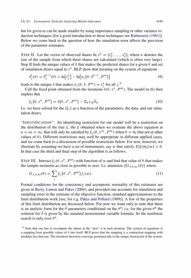
but for given ns can be made smaller by using importance sampling or other variance re-duction techniques [for a good introduction to these techniques see Rubinstein (1981)].Below we come back to the question of how the simulation error affects the precisionof the parameter estimates.
STEP II. Let the vector of observed shares be sn = [sn1 , . . . , sn
J ], where n denotes thesize of the sample from which these shares are calculated (which is often very large).Step II finds the unique values of δ that makes the predicted shares for a given θ and setof simulation draws equal to sn. BLP show that iterating on the system of equations
(9)δkj (θ) = δk−1
j (θ) + ln[snj
]− ln[σj
(θ, δk−1, P ns)]
leads to the unique δ that makes σj (θ, δ, P ns) = snj for all j .9
Call the fixed point obtained from the iterations δ(θ, sn, P ns). The model in (6) thenimplies that
(10)ξj
(θ, sn, P ns) = δ
(θ, sn, P ns)− �kxjkθk.
I.e. we have solved for the {ξj } as a function of the parameters, the data, and our simu-lation draws.
“IDENTIFICATION”. An identifying restriction for our model will be a restriction onthe distribution of the true ξ , the ξ obtained when we evaluate the above equation atn = ns = ∞, that will only be satisfied by ξj (θ, s∞, P ∞) when θ = θ0 (but not at othervalues of θ ). Different restrictions may well be appropriate in different applied cases,and we come back to a discussion of possible restrictions below. For now, however, weillustrate by assuming we have a set of instruments, say w that satisfy E[ξ(θ0)|w] = 0.In that case the third and final step of the algorithm is as follows.
STEP III. Interact ξj (θ, sn, P ns) with function of w and find that value of θ that makesthe sample moments as close as possible to zero. I.e. minimize ‖GJ,n,ns(θ)‖ where
(11)GJ,n,ns(θ) =∑j
ξj
(θ, sn, P ns)fj (w).
Formal conditions for the consistency and asymptotic normality of this estimator aregiven in Berry, Linton and Pakes (2004), and provided one accounts for simulation andsampling error in the estimate of the objective function, standard approximations to thelimit distribution work [see, for e.g. Pakes and Pollard (1989)]. A few of the propertiesof this limit distribution are discussed below. For now we want only to note that thereis an analytic form for the θ parameters conditional on the θu; i.e. for the given θu thesolution for θ is given by the standard instrumental variable formula. So the nonlinearsearch is only over θu.
9 Note that one has to recompute the shares at the “new” δ at each iteration. The system of equations isa mapping from possible values of δ into itself. BLP prove that the mapping is a contraction mapping withmodulus less that one. The iterations therefore converge geometrically to the unique fixed point of the system.

4190 D. Ackerberg et al.
1.4. Additional sources of information on demand parameters
Often we find that there is not enough information in product level demand data toestimate the entire distribution of preferences with sufficient precision. This should notbe surprising given that we are trying to estimate a whole distribution of preferencesfrom just aggregate choice probabilities. Other than functional form, the informationthat is available for this purpose comes from differences in choice sets across marketsor time periods (this allows you to sweep out preferences for given characteristics),and differences in preferences across markets or over time for a fixed choice set (thepreferences differences are usually associated with known differences in demographiccharacteristics). The literature has added information in two ways. One is to add anequilibrium assumption and work out its implications for the estimation of demandparameters, the other is to add data. We now consider each of these in turn.
1.4.1. Adding the pricing equation
There is a long tradition in economics of estimating “hedonic” or reduced form equa-tions for price against product characteristics in differentiated product markets [see, inparticular Court (1939) and Griliches (1961)]. Part of the reason those equations wereconsidered so useful, useful enough to be incorporated as correction procedures in theconstruction of most countries’ Consumer Price Indices, was that they typically hadquite high R2’s.10 Indeed, at least in the cross section, the standard pricing equationsestimated by I.O. economists have produced quite good fits (i.e. just as the model pre-dicts, goods with similar characteristics tend to sell for similar prices, and goods in partsof the characteristic space with lots of competitors tend to sell for lower prices). Perhapsit is not surprising then that when the pricing system is added to the demand system theprecision of the demand parameters estimates tends to improve noticeably (see, for e.g.BLP).
Adding the pricing system from an oligopoly model to the demand system and es-timating the parameters of two systems jointly is the analogue of adding the supplyequation to the demand equation in a perfectly competitive model and estimating theparameters of those systems jointly. So it should not be surprising that the empiricaloligopoly literature itself started by estimating the pricing and demand systems jointly[see Bresnahan (1981)]. On the other hand there is a cost of using the pricing equation.It requires two additional assumptions: (i) an assumption on the nature of equilibrium,and (ii) an assumption on the cost function.
The controversial assumption is the equilibrium assumption. Though there has beensome empirical work that tries a subset of the alternative equilibrium assumptions andsees how they fit the data [see, for e.g. Berry, Levinsohn and Pakes (1999) or Nevo
10 For a recent discussion of the relationship between hedonic regressions and pricing equations with specialemphasis on implications for the use of hedonics in the CPI, see Pakes (2004).

Ch. 63: Econometric Tools for Analyzing Market Outcomes 4191
(2001)], almost all of it has assumed static profit maximization, no uncertainty, and thatone side of the transaction has the power to set prices while the other can only decidewhether and what to buy conditional on those prices. There are many situations in whichwe should expect current prices to depend on likely future profits (e.g.’s include any sit-uation in which demand or cost tomorrow depends on current sales, and/or where thereare collusive possibilities; for more discussion see the last section of this chapter). Ad-ditionally there are many situations, particularly in markets where vertical relationshipsare important, where there are a small number of sellers facing a small number of buy-ers; situations where we do not expect one side to be able to dictate prices to another[for an attempt to handle these situations see Pakes et al. (2006)].
On the other hand many (though not all) of the implications of the results that are ofinterest will require the pricing assumption anyway, so there might be an argument forusing it directly in estimation. Moreover, as we have noted, the cross-sectional distrib-ution of prices is often quite well approximated by our simple assumptions, and, partlyas a result, use of those assumptions is often quite helpful in sorting out the relevanceof alternative values of θ .
We work with a Nash in prices, or Bertrand, assumption. Assume that marginal cost,to be denoted by mc, is log linear in a set of observables rkj and a disturbance whichdetermines productivity or ωj , i.e.
(12)ln[mcj ] =∑
rk,j θck + ωj .
r will typically include product characteristics, input prices and, possibly the quantityproduced (if there are nonconstant returns to scale). As a result our demand and costdisturbances (i.e. ξ and ω) will typically be mean independent of some of the compo-nents of r but not of others. Also we might expect a positive correlation between ξ andω since goods with a higher unobserved quality might well cost more to produce.
Since we characteristically deal with multiproduct firms, and our equilibrium as-sumption is that each firm sets each of its prices to maximize the profits from all ofits products conditional on the prices set by its competitors, we need notation for theset of products owned by firm f , say Jf . Then the Nash condition is that firms set eachof their prices to maximize
∑j∈Jf
(pj − Cj (·))Msj (·), where Cj is total costs. Thisimplies that for j = 1, . . . , J
(13)σj (·) +∑l∈Jf
(pl − mcl )M∂σl(·)∂pj
= 0.
Note that we have added a system of J equations (one for each price) and R = dim(r)
parameters to the demand system. So provided J > R we have added degrees of free-dom.
To incorporate the information in (13) and (12) into the estimation algorithm rewritethe first order condition as s + (p − mc)� = 0, where �i,j is nonzero for elements ofa row that are owned by the same firm as the row good. Then
p − mc = �−1σ(·).

4192 D. Ackerberg et al.
Now substitute from (12) to obtain the cost disturbance as
(14)ln(p − �−1σ
)− r ′θc = ω(θ),
and impose the restrictions that
Efj (w)ωj (θ) = 0 at θ = θ0.
We add the empirical analogues of these moments to the demand side momentsin (11) and proceed as in any method of moments estimation algorithm. This entailsone additional computational step. Before we added the pricing system every time weevaluated a θ we had to simulate demand and do the contraction mapping for that θ .Now we also have to calculate the markups for that θ .
1.4.2. Adding micro data
There are a number of types of micro data that might be available. Sometimes we havesurveys that match individual characteristics to a product chosen by the individual. Lessfrequently the survey also provides information on the consumer’s second choice (see,for e.g. MicroBLP), or is a panel which follows multiple choices of the same consumingunit over time. Alternatively we might not have the original survey’s individual choicedata, but only summary statistics that provide information on the joint distribution ofconsumer and product characteristics [for a good example of this see Petrin’s (2002)use of Consumer Expenditure Survey moments in his study of the benefits to the in-troduction of the minivan]. We should note that many of the micro data sets are choicebased samples, and the empirical model should be built with this in mind [see, for e.g.MicroBLP (2004); for more on the literature on choice based sampling see Manski andLerman (1977) and Imbens and Lancaster (1994)].
Since the model in (6) is a model of individual choice, it contains all the detail neededto incorporate the micro data into the estimation algorithm. Thus the probability of anindividual with observed characteristics zi choosing good j given (θ, δ) is given by
(15)
Pr(j |zi, θ, δ) =∫
ν
exp[δj + �klxjkzilθokl + �klxjkνilθ
ukl]
1 +∑q exp[δq + �klxqkzilθokl + �klxjkνilθ
ukl]
f (ν) d(ν).
1.4.2.1. What can be learned from micro data Assume temporarily that we can actu-ally compute the probabilities in (15) analytically. Then we can use maximum likelihoodto estimate (θo, θu). These estimates do not depend on any restrictions on the distribu-tion of ξ . I.e. by estimating free δj coefficients, we are allowing for a free set of ξj .
On the other hand recall that
δj = �kxjkθk + ξj .
So we cannot analyze many of the implications of the model (including own and crossprice elasticities) without a further assumption which enables us to separate out the

Ch. 63: Econometric Tools for Analyzing Market Outcomes 4193
effect of ξ from the effect of the x on δ (i.e. without the identifying assumption referredto above). The availability of micro data, then, does not solve the simultaneity problem.In particular, it does not enable us to separate out the effect of price from unobservablecharacteristics in determining aggregate demand. On the other hand there are a fewimplications of the model that can be analyzed from just the estimates of (δ, θo, θu).In particular, estimates of consumer surplus from the products currently marketed (andhence “ideal” consumer price indices) depend only on these parameters, and hence donot require the additional identifying assumption.
Now say we wanted to use the data to estimate θ . In order to do so we need a furtherrestriction so assume, as before, that we have instruments w, and can provide instru-mental variable estimates of the θ . The number of observations for the instrumentalvariable regressions is the number of products. That is, at least if we chose to estimate(θo, θu) without imposing any constraints on the distribution of ξ , the precision of theestimates of θ will depend only on the richness of the product level data. Moreover,IV regressions from a single cross-section of products in a given market are not likelyto produce very precise results; in particular there is likely to be very little independentvariance in prices. Since additional market level data is often widely available, this ar-gues for integrating it with the micro data, and doing an integrated analysis of the twodata sources.
One more conceptual point on survey data. What the survey data adds is informationon the joint distribution of observed product and consumer attributes. We would expectthis to be very helpful in estimating θo, the parameters that determine the interactionsbetween z and x. There is a sense in which it also provides information on θu, but thatinformation is likely to be much less precise. That is we can analyze the variance inpurchases among individuals with the same choice set and the same value of z and usethat, together with the i.i.d. structure of the ε, to try and sort out the variance-covarianceof the ν. However this requires estimates of variances conditional on z, and in practicesuch estimates are often quite imprecise. This is another reason for augmenting cross-sectional survey data with aggregate data on multiple markets (or time periods) in anintegrated estimation routine; then the observed variance in z could determine the θo
and differences in choice sets could help sweep out the impact of the θu parameter.When the data does have second choice information, or when we observe the same
consuming unit purchasing more than one product, there is likely to be much moredirect information on θu. This because the correlation between the x-intensity of thefirst choice and the second choice of a given individual is a function of both θo and theθu terms, and the θo terms should be able to be estimated from only the first choicedata. A similar comment can be made for repeated choices, at least provided the utilityfunction of the consuming unit does not change from choice to choice.
Table 2 illustrates some of these points. It is taken from MicroBLP where the dataconsisted of a single cross-sectional survey of households, and the market level datafrom the same year. The survey contained information on household income, the numberof adults, the number of children, the age (of the head) of household, and whether theirresidence was rural, urban, or suburban (and all of these were used in the estimation).

4194 D. Ackerberg et al.
Table 2Price substitutes for selected vehicles, a comparison among models
Vehicle Full model Logit 1st Logit 1st and 2nd Sigma only
Metro Tercel Caravan Ford FS PU CivicCavalier Escort Caravan Ford FS PU EscortEscort Tempo Caravan Ford FS PU RangerCorolla Escort Caravan Ford FS PU CivicSentra Civic Caravan Ford FS PU CivicAccord Camry Caravan Ford FS PU CamryTaurus Accord Caravan Ford FS PU AccordLegend Town Car Caravan Ford FS PU LinTncSeville Deville Caravan Ford FS PU DevilleLex LS400 MB 300 Econovan Ford FS PU SevilleCaravan Voyager Voyager Voyager VoyagerQuest Aerostar Caravan Caravan AerostarG Cherokee Explorer Caravan Chv FS PU ExplorerTrooper Explorer Caravan Chv FS PU RodeoGMC FS PU Chv FS PU Caravan Chv FS PU Chv FS PUToyota PU Ranger Caravan Chv FS PU RangerEconovan Dodge Van Caravan Ford FS PU Dodge Van
Source: From Berry, Levinsohn and Pakes (2004).
That study had particularly rich information on vehicle preferences, as each householdreported its second as well as its first best choice.
Table 2 provides the best price substitutes for selected models from demand systemsfor automobiles that were estimated in four different ways: (i) the full model allowsfor both the zi and the νi (i.e. for interactions between both observed and unobservedindividual characteristics and product characteristics), (ii) the logit models that allow foronly the zi , and (iii) the σ ’s only model allows for only the νi . The most important pointto note is that without allowing for the νi there is a clear IIA problem. The prevalence ofthe Caravan and the Full Size (FS) pickups when we use the logit estimates (the modelswithout the νi) is a result of them being the vehicles with the largest market sharesand the apparent absence of the observed factors which cause different households toprefer different product characteristics differentially. Comparing to column (iv) it isclear that the extent of preference heterogeneity caused by household attributes not inour data is large. MicroBLP also notes that when they tried to estimate the full modelwithout the second choice information their estimates of the θu parameters were veryimprecise; too imprecise to present. However when they added the second choice datathey obtained both rather precise estimates of the contributions of the unobserved factorsand substitution patterns that made quite a bit of sense. Finally we note that the fact thatthere was only a single year’s worth of data made the estimates of θ quite imprecise,and the paper uses other sources of information to estimate those parameters.

Ch. 63: Econometric Tools for Analyzing Market Outcomes 4195
1.4.2.2. Computational and estimation issues: Micro data There are a number ofchoices to make here. At least in principal we could (i) estimate (θo, θu, δ) pointwise,or (ii) make an assumption on the distribution of ξ (e.g. E[ξ |w] = 0), and estimate(θo, θu, θ) instead of (θo, θu, δ). However the fact that ξ is a determinant of price, andprice is in the x vector, makes it difficult to operationalize (ii). To do so it seems thatone would have to make an assumption on the primitive distribution of ξ , solve outfor equilibrium prices conditional on (θ, ξ, x), substitute that solution into the choiceprobabilities in (15), and then use simulation to integrate out the ξ and ν in the formulafor those probabilities. This both involves additional assumptions and is extremely de-manding computationally. The first procedure also has the advantage that its estimatesof (θo, θu) are independent of the identifying restriction used to separate out the effectof ξ from the effect of x on θ .
Assume that we do estimate (θo, θu, δ). If there are a large number of products or J ,this will be a large dimensional search (recall that there are J components of δ), andlarge dimensional searches are difficult computationally. One way to overcome thisproblem is to use the aggregate data to estimate δ conditional on θ from the contractionmapping in (9), and restrict the nonlinear search to searching for (θo, θu).
Finally since the probabilities in (15) are not analytic, either they, or some transformof them (like the score), will have to be simulated. There is now quite a bit of work onsimulating the probabilities of a random coefficient logit model [see Train (2003) andthe literature cited there]. Here we only want to remind the reader that in the applicationswe have in mind it is likely to be difficult to use the log (or a related) function of thesimulated probabilities in the objective function. Recall that if pns(θ) is the simulatedprobability, and pns(θ) = p(θ) + ens, where ens is a zero mean simulation error, then
log[pns(θ)
] ≈ log[p(θ)
]+ ens
p(θ)− (ens)2
2 × p(θ)2.
So if the simulated probabilities are based on ns independent simulation draws eachof which has variance V (p(θ)) the bias in the estimate of the log probability will beapproximately
E log[pns(θ)
]− log[p(θ)
] ≈ − 1
2 × ns × p(θ),
and ns must be large relative to p(θ) for this bias to go away (this uses the fact thatVar(pns(θ)) ≈ p(θ)/ns).
In many Industrial Organization problems the majority of the population do not pur-chase the good in a given period, and the probabilities of the inside goods are formedby distributing the remainder of the population among a very large number of goods.For example, in MicroBLP’s auto example, only ten per cent of households purchase acar in the survey year, and that ten percent is distributed among more than two hundredmodels of cars. So it was common to have probabilities on the order of 10−4. It shouldnot be a surprise then that they chose to fit moments which were linear functions ofthe error in estimating the probabilities (they fit the covariances of car characteristics

4196 D. Ackerberg et al.
and household characteristics predicted by the model to those in the data) rather thanmaximizing a simulated likelihood.
1.4.3. Identifying restrictions
Recall that the source of the endogeneity problem in the demand estimates is thecorrelation of the product specific unobservable, our ξ , with some of the observablecharacteristics of the product; in particular we are worried about a correlation of ξ withprice. The contraction mapping in (9) is helpful in this respect as it delivers ξ as a linearfunction of observables. As a result, any of the standard ways of solving endogeneityproblems in linear models can be employed here.
The most familiar way of dealing with endogeneity problems in linear models is touse instruments. The question then becomes what is an appropriate instrument for x’sin the demand system, a question which has been discussed extensively in the contextof perfectly competitive models of supply and demand. As in those models cost shiftersthat are excluded from demand and uncorrelated with the demand error are available asinstruments. The familiar problem here is that input prices typically do not vary much;at least not within a single market. There are a couple of important exceptions. Oneis when production takes place in different locations even though the products are allsold in one market [as is common when investigating trade related issues, see Berry,Levinsohn and Pakes (1999)]. Another is when a subset of the x’s are exogenous, thecost factors are differentially related to different x’s, and the x-intensity of differentproduct varies. In this case interactions between the cost factors and those x’s should beuseful instruments.
In addition to cost instruments, Nevo (2001) uses an idea from Hausman (1996)market-equilibrium version of the AIDS model, applied to a time-series/cross-sectionpanel of geographically dispersed set of markets. The underlying assumption is that de-mand shocks are not correlated across markets while cost shocks are correlated acrossmarkets. The prices of goods in other markets then become instruments for the price ofgoods in a given market. Nevo (2001) studies breakfast cereals and so sources of com-mon cost shocks include changes in input prices; sources of common demand shocks(which are ruled out) include national advertising campaigns.
In oligopoly markets prices typically sell at a markup over marginal cost. So if theproduct’s own (xj , rj )’s are used as instruments, then so might the (x−j , r−j ) of otherproducts, giving us a lot of potential instruments. Moreover, if price setting models likethe one in Equation (13) are appropriate (and recall that they often have a lot of explana-tory power), the impact of the (x−j , r−j ) on pj will depend on whether the product’sare owned by the same or by different firms. This type of reasoning dates back at leastto Bresnahan (1987), who notes the empirical importance of the idea that markups willbe lower in “crowded” parts of the product space and that they will be higher when“nearby” products are owned by the same firm. BLP and Berry, Levinsohn and Pakes(1999) rely on this sort of argument to propose the use of functions of rivals’ observedproduct characteristics, and of the ownership structure of products, as instruments. Re-
Ch. 63: Econometric Tools for Analyzing Market Outcomes 4197
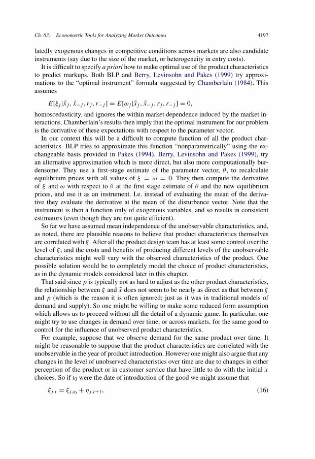
latedly exogenous changes in competitive conditions across markets are also candidateinstruments (say due to the size of the market, or heterogeneity in entry costs).
It is difficult to specify a priori how to make optimal use of the product characteristicsto predict markups. Both BLP and Berry, Levinsohn and Pakes (1999) try approxi-mations to the “optimal instrument” formula suggested by Chamberlain (1984). Thisassumes
E[ξj |xj , x−j , rj , r−j ] = E[ωj |xj , x−j , rj , r−j ] = 0,
homoscedasticity, and ignores the within market dependence induced by the market in-teractions. Chamberlain’s results then imply that the optimal instrument for our problemis the derivative of these expectations with respect to the parameter vector.
In our context this will be a difficult to compute function of all the product char-acteristics. BLP tries to approximate this function “nonparametrically” using the ex-changeable basis provided in Pakes (1994). Berry, Levinsohn and Pakes (1999), tryan alternative approximation which is more direct, but also more computationally bur-densome. They use a first-stage estimate of the parameter vector, θ , to recalculateequilibrium prices with all values of ξ = ω = 0. They then compute the derivativeof ξ and ω with respect to θ at the first stage estimate of θ and the new equilibriumprices, and use it as an instrument. I.e. instead of evaluating the mean of the deriva-tive they evaluate the derivative at the mean of the disturbance vector. Note that theinstrument is then a function only of exogenous variables, and so results in consistentestimators (even though they are not quite efficient).
So far we have assumed mean independence of the unobservable characteristics, and,as noted, there are plausible reasons to believe that product characteristics themselvesare correlated with ξ . After all the product design team has at least some control over thelevel of ξ , and the costs and benefits of producing different levels of the unobservablecharacteristics might well vary with the observed characteristics of the product. Onepossible solution would be to completely model the choice of product characteristics,as in the dynamic models considered later in this chapter.
That said since p is typically not as hard to adjust as the other product characteristics,the relationship between ξ and x does not seem to be nearly as direct as that between ξ
and p (which is the reason it is often ignored; just as it was in traditional models ofdemand and supply). So one might be willing to make some reduced form assumptionwhich allows us to proceed without all the detail of a dynamic game. In particular, onemight try to use changes in demand over time, or across markets, for the same good tocontrol for the influence of unobserved product characteristics.
For example, suppose that we observe demand for the same product over time. Itmight be reasonable to suppose that the product characteristics are correlated with theunobservable in the year of product introduction. However one might also argue that anychanges in the level of unobserved characteristics over time are due to changes in eitherperception of the product or in customer service that have little to do with the initial x
choices. So if t0 were the date of introduction of the good we might assume that
(16)ξj,t = ξj,t0 + ηj,t+1,

4198 D. Ackerberg et al.
where ηj,t+1 is mean independent of the observed characteristics of all products. Alter-natively we could assume that ξj,t followed a first order Markov process with only ξj,t0 ,and not the increments in the process, correlated with observed characteristics.
Relatedly if the data contains sales of the same product in many markets one couldthink of restrictions on how the unobservable for a single product changes across mar-kets. The most straightforward example of this is to require ξ to be the same acrossmarkets. This is quite a powerful restriction, and one might question it on the basis ofdifferences in the distribution of consumer preferences across markets that impact ontheir estimated ξ ’s. A weaker assumption would be that the difference between ξ ’s forthe same product across markets is uncorrelated with the observed x. Similarly, someproducts within a market may differ only by the addition of some optional features andwe could restrict the way that ξ changes across products that vary only in their options.
1.5. Problems with the framework
We have motivated our discussion on demand estimation by noting how the recent liter-ature dealt with the problems that arose in using representative agent models in productspace. There are many senses, however, in which the framework outlined above can betoo restrictive for particular problems. This section reviews some of the more obviousof them. The impact of these problems depend upon the market one is analyzing and theissues one is focusing on. Also, at least partial solutions to some of these problems areavailable, and we will direct the reader to them where we can. In large part, however,this section is an outline of agendas for future research on demand estimation for I.O.problems.
We begin with multiple choice and/or dynamics, and then come back to the prob-lem in the static discrete choice model considered above. Most empirical studies simplyignore issues related to multiple choices and/or dynamics. The hope is that the esti-mated demand system is still the best currently available approximation for analyzingthe question of interest. To us the surprising part of the results of those studies is that theframework seems to provide a “reasonable” approximation to substitution patterns, andeven more surprisingly, a reasonable approximation to pricing patterns. This despite thefact that we know that consumers’ demands and the market equilibrium outcomes areproducts of much more complicated processes than those we model. Even so, as willbecome clear presently, there are a number of issues of importance to I.O. which cannotbe studied empirically without a more detailed understanding of multiple choice and/orthe dynamic aspects of demand.
Multiple units of demand
There are many situations for which a model based on the choice of either one or zerounits of a good does not match reality.11 Models for choosing a finite number of units
11 Dubin and McFadden (1984) provide an earlier example with one discrete choice and one continuouschoice.

Ch. 63: Econometric Tools for Analyzing Market Outcomes 4199
from a set of substitute goods require a specification for the utility from multiple units.Then, at least in principle, we are back to a discrete choice for “tuples” of goods. How-ever to maintain tractability when the number of units can grow large the specificationis likely to require constraints which cut down the choice set by implying that somechoices are dominated by others (otherwise the size of the choice set grows as JC ,where J is the number of products and C is the maximum number of purchases).
One example of the use of such constraints is Hendel’s (1999) two-stage multiple-unit/multiple good framework for the demand of a firm for computers. He simplifies theproblem by imagining that the firm faces a random, discrete number of tasks. For eachtask, it chooses only one type (brand) of computer and, according to the random size ofthe tasks, a number of computers to purchase. This explicitly accounts for decisions topurchase multiple units of multiple kinds of goods.
Gentzkow (2004) considers a problem with a small number of goods, but where thereare a small number of choices. In that study of online and print newspapers, some of thegoods are potentially complements, and this requires a different set of modifications.Moreover, as Gentzkow shows the determination of whether goods are in fact comple-ments or substitutes interacts with the issue of the form of consumer heterogeneity insubtle ways reminiscent of the initial condition problems in panel data estimation [seeHeckman (1981)].
A related problem involves continuous choice over multiple goods. If all goods arepurchased in some positive amount by every consumer, then a traditional continuousdemand approach, equating marginal rates of substitution across all goods, is appropri-ate. But many real-world consumer data problems involve a large number of goods withmany zero purchase decisions and many positive purchase decisions. Chan (2002) con-siders the Kuhn–Tucker version of the traditional continuous choice problem to studysoft drink purchases.
Dynamic demand
Yet another set of problems arises when the demand for the good is inherently dynamic,as occurs with either durable, storable, or experience goods. Models which are appro-priate for dynamic demand estimation can become quite complex; they require forwardlooking consumers whose behavior depends on the likely distribution of future (as wellas current) offerings. Moreover, in a complete model these future offerings would, inturn, depend on producer’s perceptions of consumer demand. A number of new studiesmake simplifying assumptions which allow them to make some headway.
Both Hendel and Nevo (2002) and Erdem, Imai and Keane (2003) consider a problemof durable good demand in an explicitly dynamic framework. They consider shoppingdecisions when consumers are allowed to store purchases, and use a reduced form as-sumption on the process generating prices. It has been clear to I.O. economists for sometime that we are going to have to model intertemporal substitution of this form in orderto understand “sales” in retail markets [see Sobel (1984)].

4200 D. Ackerberg et al.
Two problems in this kind of study are that the rate of consumption (inventory re-duction) at home is typically not observed and the dimension of the state space (whichinvolves both the current price vector, which predicts future prices, and also the vectorof household inventories of different brands). In these models new purchases are addedto a single-index of home inventories, with different brands of product receiving differ-ent utility weights in the inventory stock. This single index of inventories reduces thedimensionality of the state space. Another simplifying assumption is that unobservedhousehold consumption follows a simple rule.
Esteban and Shum (2002) consider a model of durable automobile purchases. Theyassume a used-car market with zero transaction costs. The zero transaction costs implythat the joint distribution of past choices and consumer characteristics are not a statevariable of the problem. Under these assumptions they are able to derive empirical im-plications about the dynamic pricing problem of the durable goods manufacturer (indetermining current price the manufacturer has to worry about future aggregate supplyof the used goods). Many, if not most, manufacturing goods are durable.
Studies of demand for advertised experience goods include Erdem and Keane (1996),Ackerberg (2003), and Crawford and Shum (2007). All of these papers feature Bayesianconsumers who learn both from experience and from adverting. This leads to a fairlycomplex dynamic programming problems for the consumer. The studies largely ignorethe firm’s endogenous pricing and advertising decisions.
Problems with the static discrete choice specification
There are also aspects of the static discrete choice specification of the model outlinedabove whose flexibility, and/or implications, are not yet well understood. One suchissue is whether the second derivatives of the demand function are very flexibly es-timated. This will determine whether two goods are strategic substitutes or strategiccomplements, and hence has implications for the analysis of the structure of strategicinteraction, and appears to be largely unexplored in the current literature. More gen-erally there are a host of questions on what we can learn nonparametrically about thestructure of demand from different kinds of data that we have not touched on here (fora discussion of some of them, see Matzkin’s contribution to this volume).
A second such issue concerns the role of the i.i.d. “idiosyncratic match values”, theεij ’s, in the models above. These are added to the model largely for computational con-venience; they do not seem to match any omitted causal demand determinant. Moreover,the presence of the εij has implications. They imply that each product is “born” with adistribution of consumer tastes whose conditional distribution, conditional on the tastesfor other products, has support that ranges from minus to plus infinity. This implies thatevery conceivable product, no matter its characteristics and price, will have a strictlypositive (though perhaps quite tiny) expected market share.
Given the standard εij ’s, each product will also have a positive cross-price effect withevery other product: competition is never completely local. Perhaps most problematic,it also implies that if we define a consumer by a (z, ν) combination, every consumer’s
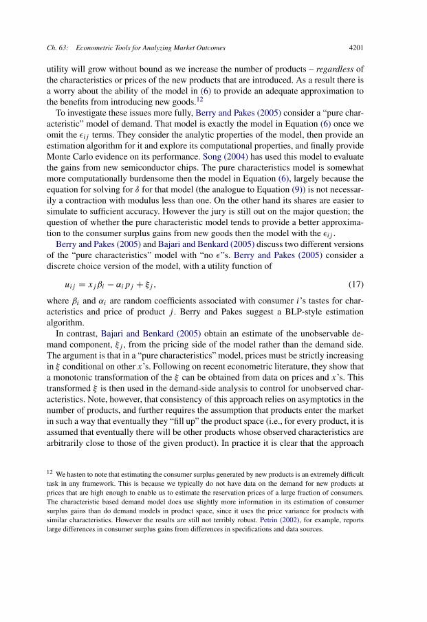
Ch. 63: Econometric Tools for Analyzing Market Outcomes 4201
utility will grow without bound as we increase the number of products – regardless ofthe characteristics or prices of the new products that are introduced. As a result there isa worry about the ability of the model in (6) to provide an adequate approximation tothe benefits from introducing new goods.12
To investigate these issues more fully, Berry and Pakes (2005) consider a “pure char-acteristic” model of demand. That model is exactly the model in Equation (6) once weomit the εij terms. They consider the analytic properties of the model, then provide anestimation algorithm for it and explore its computational properties, and finally provideMonte Carlo evidence on its performance. Song (2004) has used this model to evaluatethe gains from new semiconductor chips. The pure characteristics model is somewhatmore computationally burdensome then the model in Equation (6), largely because theequation for solving for δ for that model (the analogue to Equation (9)) is not necessar-ily a contraction with modulus less than one. On the other hand its shares are easier tosimulate to sufficient accuracy. However the jury is still out on the major question; thequestion of whether the pure characteristic model tends to provide a better approxima-tion to the consumer surplus gains from new goods then the model with the εij .
Berry and Pakes (2005) and Bajari and Benkard (2005) discuss two different versionsof the “pure characteristics” model with “no ε”s. Berry and Pakes (2005) consider adiscrete choice version of the model, with a utility function of
(17)uij = xjβi − αipj + ξj ,
where βi and αi are random coefficients associated with consumer i’s tastes for char-acteristics and price of product j . Berry and Pakes suggest a BLP-style estimationalgorithm.
In contrast, Bajari and Benkard (2005) obtain an estimate of the unobservable de-mand component, ξj , from the pricing side of the model rather than the demand side.The argument is that in a “pure characteristics” model, prices must be strictly increasingin ξ conditional on other x’s. Following on recent econometric literature, they show thata monotonic transformation of the ξ can be obtained from data on prices and x’s. Thistransformed ξ is then used in the demand-side analysis to control for unobserved char-acteristics. Note, however, that consistency of this approach relies on asymptotics in thenumber of products, and further requires the assumption that products enter the marketin such a way that eventually they “fill up” the product space (i.e., for every product, it isassumed that eventually there will be other products whose observed characteristics arearbitrarily close to those of the given product). In practice it is clear that the approach
12 We hasten to note that estimating the consumer surplus generated by new products is an extremely difficulttask in any framework. This is because we typically do not have data on the demand for new products atprices that are high enough to enable us to estimate the reservation prices of a large fraction of consumers.The characteristic based demand model does use slightly more information in its estimation of consumersurplus gains than do demand models in product space, since it uses the price variance for products withsimilar characteristics. However the results are still not terribly robust. Petrin (2002), for example, reportslarge differences in consumer surplus gains from differences in specifications and data sources.

4202 D. Ackerberg et al.
requires data with many products per market, but there has not been enough experienceto date to know what “many” means in this context.
1.6. Econometric details
This subsection summarizes results from Berry, Linton and Pakes (2004) who providelimit theorems for the parameter estimates from differentiated product models. The ac-tual form of the limit distributions depends on the type of data and type of model. Wewill focus on the case where only one cross section of market level data is available.Our purpose is to give the reader some indication of how the various estimation errorsthat have been introduced are likely to effect the parameter estimates, and this is thesimplest environment in which to show that.13
Recall that the objective function minimized in the estimation algorithm or Equa-tion (11) is a norm of
GJ
(θ, sn, P ns) = 1
J
J∑j=1
ξj
(θ, sn, P ns)fj (w).
The ξj are defined implicitly as the solution to the system
snj = σj
(ξ, x; θ, P ns),
where σ(·) is defined in (8), the w satisfy E[ξ |w, θ0] = 0, sn is the observed vector ofmarket shares, and P ns is notation for the vector of simulation draws used to computethe market shares predicted by the model.
The objective function, ‖GJ (θ, sn, P ns)‖, has a distribution determined by threeindependent sources of randomness: randomness generated from the draws on the prod-uct characteristics (both observed and unobserved, in the full model these are vectors{ξ, x, r, ω}), randomness generated from the sampling distribution of sn, and that gen-erated from the simulated distribution P ns. Analogously there are three dimensions inwhich our sample can grow: as n, as ns, and as J grow large.
The limit theorems allow different rates of growth for each dimension. Throughoutwe take pathwise limits, i.e. we write n(J ) and ns(J ), let J → ∞, and note that ourassumptions imply n(J ), ns(J ) → ∞ at some specified rate. Note also that both sn
and σ(ξ, θ, P ) take values in RJ , where J is one of the dimensions that we let grow inour limiting arguments. This is an unusual feature of the econometric model and causescomplications in the limiting arguments. As will become obvious sampling error (error
13 Cases in which there is data from many regional markets but the same goods are sold in each of them willstill have to deal with limits as the number of products grows large; it is just that then we might also wantto let the number of markets increase as we increase the number of products. Also in cases with regionalmarkets the computational problems we highlight will be even more severe, as then we will have to computeξ separately in each different market.

Ch. 63: Econometric Tools for Analyzing Market Outcomes 4203
in sn) plays an analogous role to simulation error (error in P ns), so for notational sim-plicity assume that n is sufficiently large that we do not need to worry about samplingerror. When there is no sampling (simulation) error we set n (ns) equal to zero.
We need to find an approximation for the objective function which allows us to sep-arate out the roles of the three sources of error. To this end write
(18)ξ(θ, s0, P ns) = ξ
(θ, s0, P 0)+ {ξ(θ, s0, P ns)− ξ
(θ, s0, P 0)}.
The function σ(ξ, θ, P ) is differentiable in ξ , and its derivative has an inverse, say
H−1(ξ, θ, P ) ={
∂σ (ξ, θ, P )
∂ξ ′
}−1
.
Abbreviate σo(θ, s, P ) = σ(ξ(s, θ, P ), θ, P ) and Ho(θ, s, P ) = H(ξ(s, θ, P ), θ, P ),and let
σ(ξ, P ns, θ
) = σ(ξ, P 0, θ
)+ εns(θ).
Then from the fact that we obtain ξ from σ(·) = σ(ξ, P 0, θ) + εns(θ) it follows that
ξ(θ, s0, P ns) = ξ
(θ, s0, P 0)+ H−1
o
(θ, s0, P 0){εns(θ)
}+ r(θ, sn, P ns),
where r(θ, sn, P ns) is a remainder term. Substituting into (18)
GJ
(θ, sn, P ns) = GJ
(θ, s0, P 0)+ 1
Jz′H−1
o
(θ, s0, P 0){−εns(θ)
}+ 1
Jz′r(θ, sn, P ns).
The limit theorems in Berry, Linton and Pakes (2004) work from this representa-tion of GJ (θ, sn, P ns). To prove consistency they provide conditions which insure that:(i) the second and third terms in this equation converge to zero in probability uniformlyin θ , and (ii) an estimator which minimized ‖GJ (θ, s0, P 0)‖ over θ ∈ Θ would lead toa consistent estimator of θ0.
Asymptotic normality requires, in addition, local regularity conditions of standardform, and a limiting distribution for H−1
o (θ, s0, P 0){−εns(θ)}. The rate needed for thislimit distribution depends on how the elements of the J × J matrix H−1
o (θ, s0, P 0)
grow, as J gets large. It is easiest to illustrate the issues that can arise here by goingback to the simple logit model.
In that model: ui,j = δj + εi,j , with the {εi,j } distributed i.i.d. type II extreme value,and δj = xj θ + ξj . Familiar arguments show that σj = exp[δj ]/(1 + ∑q exp[δq ]),while σ0 = 1/(1 +∑q exp[δq ]). In this case the solution to the contraction mappingin (9) is analytic and
ξj
(θ, so, P o
) = (ln[soj
]− ln[so
0
])− xjβ.
Thus in this simple case
∂ξ
∂sj
∣∣∣∣so
= 1
soj
.
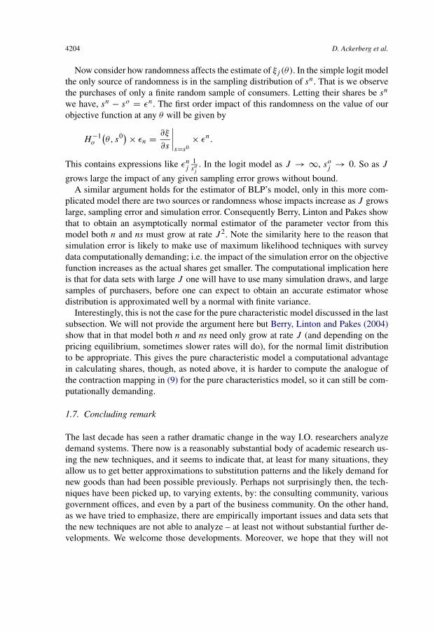
4204 D. Ackerberg et al.
Now consider how randomness affects the estimate of ξj (θ). In the simple logit modelthe only source of randomness is in the sampling distribution of sn. That is we observethe purchases of only a finite random sample of consumers. Letting their shares be sn
we have, sn − so = εn. The first order impact of this randomness on the value of ourobjective function at any θ will be given by
H−1o
(θ, s0)× εn = ∂ξ
∂s
∣∣∣∣s=s0
× εn.
This contains expressions like εnj
1soj
. In the logit model as J → ∞, soj → 0. So as J
grows large the impact of any given sampling error grows without bound.A similar argument holds for the estimator of BLP’s model, only in this more com-
plicated model there are two sources or randomness whose impacts increase as J growslarge, sampling error and simulation error. Consequently Berry, Linton and Pakes showthat to obtain an asymptotically normal estimator of the parameter vector from thismodel both n and ns must grow at rate J 2. Note the similarity here to the reason thatsimulation error is likely to make use of maximum likelihood techniques with surveydata computationally demanding; i.e. the impact of the simulation error on the objectivefunction increases as the actual shares get smaller. The computational implication hereis that for data sets with large J one will have to use many simulation draws, and largesamples of purchasers, before one can expect to obtain an accurate estimator whosedistribution is approximated well by a normal with finite variance.
Interestingly, this is not the case for the pure characteristic model discussed in the lastsubsection. We will not provide the argument here but Berry, Linton and Pakes (2004)show that in that model both n and ns need only grow at rate J (and depending on thepricing equilibrium, sometimes slower rates will do), for the normal limit distributionto be appropriate. This gives the pure characteristic model a computational advantagein calculating shares, though, as noted above, it is harder to compute the analogue ofthe contraction mapping in (9) for the pure characteristics model, so it can still be com-putationally demanding.
1.7. Concluding remark
The last decade has seen a rather dramatic change in the way I.O. researchers analyzedemand systems. There now is a reasonably substantial body of academic research us-ing the new techniques, and it seems to indicate that, at least for many situations, theyallow us to get better approximations to substitution patterns and the likely demand fornew goods than had been possible previously. Perhaps not surprisingly then, the tech-niques have been picked up, to varying extents, by: the consulting community, variousgovernment offices, and even by a part of the business community. On the other hand,as we have tried to emphasize, there are empirically important issues and data sets thatthe new techniques are not able to analyze – at least not without substantial further de-velopments. We welcome those developments. Moreover, we hope that they will not

Ch. 63: Econometric Tools for Analyzing Market Outcomes 4205
be judged by any absolute criteria but rather by the simple test of whether they allowfor improvements in our ability to empirically analyze one or more issue of substantiveinterest.
2. Production functions
As noted in the introduction, the advent of new micro data sets on the inputs and out-puts from the production process has generated a renewed interest in the estimation ofproduction functions and their use in the analysis of productivity. We begin this sec-tion by reviewing the basic simultaneity and selection issues that the recent literature onproduction function estimation has faced. We then consider the traditional solutions tothese issues, pointing out why those solutions are not likely to be terribly helpful in ourcontext.
Next we introduce an approach based on explicit models of input choices and exitdecisions that was first introduced in a paper by Olley and Pakes (1996). Our presenta-tion of the Olley–Pakes model will stress the assumptions they used which either we,or others before us, see as questionable (at least in certain environments). These in-clude assumptions on: the timing of input choices, the cost of changing the levels ofdifferent inputs over time, the process by which productivity evolves over time, and therelationship of investment to that process. The rest of the section focuses on ways oftesting these assumptions, and details recently proposed modifications to the estimationprocedure which might be used when they seem appropriate.
2.1. Basic econometric endogeneity issues
We can illustrate all issues that will concern us with simple Cobb–Douglas productiontechnology
Yj = AjKβk
j Lβl
j
with one output (Yj ) and two inputs; capital (Kj ) and labor (Lj ). Aj represents theHicksian neutral efficiency level of firm j , which is unobserved by the econometri-cian.14
Taking natural logs results in a linear equation
(19)yj = β0 + βkkj + βllj + εj ,
where lowercase symbols represent natural logs of variables and ln(Aj ) = β0 + εj .The constant term β0 can be interpreted as the mean efficiency level across firms, while
14 The methods discussed in this chapter are equally applicable to many other production functions. As weshall see the major requirements will be that variable inputs have positive cross-partials with productivity, andthat the value of the firm is increasing in fixed inputs.

4206 D. Ackerberg et al.
εj is the deviation from that mean for firm j . εj might represent innate technology ormanagement differences between firms, measurement errors in output, or unobservedsources of variance in output caused by weather, machine breakdowns, labor problems,etc.
We have known since Marschak and Andrews (1944) that direct OLS estimationof (19) is problematic. The problem is that the right-hand side variables, capital andlabor, are generally chosen by the firm. If the firm has knowledge of its εj (or some partof εj ) when making these input choices, the choices will likely be correlated with εj .For example, suppose that firms operate in perfectly competitive input and output mar-kets (wj , rj , and pj being the prices of labor, capital, and output, respectively), thatcapital is a fixed input, that firms perfectly observe εj before choosing labor, and thatfirms’ current choices of labor only impact current profits and have no effect on futureprofits. Then the firm’s optimal short-run choice of labor input is given by
(20)Lj =[
pj
wj
βleβ0+εj K
βk
j
] 11−βl
.
Since choice of Lj (and thus lj ) depends directly on εj , OLS will generate biasedcoefficient estimates. In more general models, firms’ choices of Kj will also typicallybe correlated with εj .15
There is a second, less well documented, endogeneity problem often inherent in OLSestimation of (19). Firm level datasets usually have a considerable level of attrition. Forexample, over a wide range of manufacturing industries, Dunne, Roberts and Samuelson(1988) find exit rates higher than 30% between 5 year census pairs. In applied work,one only has data on firms prior to exiting. If firms have some knowledge of εj prior toexiting, the firms that continue to produce will have εj draws from a selected sample,and the selection criteria will be partially determined by the other fixed inputs. Againas a simple example, suppose that firms are monopolies that are exogenously endowedwith different fixed levels of capital. Firms then observe εj , decide whether to exit ornot, and choose labor and produce if they have not exited. Also for simplicity supposethat after production firms disappear, so that the firms have no dynamic considerations.Firms in this situation will have an exit rule of the following form:
χ(εj ,Kj ; pj ,wj , β) = 0 (or exit) iff Π(εj ,Kj ; pj ,wj , β) < Ψ,
where β is the set of parameters (β0, βl, βk) and Ψ is the nonnegative selloff value of thefirm. Π is the argmax (over the variable input labor) of variable profits. This conditionstates that firms exit if variable profits are not at least as high as the selloff value of thefirm.16
15 Empirical results have lead practitioners to conclude that most often the bias imparted on the labor coeffi-cient βl is larger than the bias imparted on the capital coefficient βk . This is consistent with models of inputchoice where labor is more easily adjustable than capital (i.e. labor is a “more variable” input than capital).The intuition here is that because it is more quickly adjustable, labor is more highly correlated with εj .16 This is a very simple example of an exit rule. More realistic models of exit would be dynamic in natureand distinguish between fixed and sunk costs; see the discussion below.

Ch. 63: Econometric Tools for Analyzing Market Outcomes 4207
The key point is that this exit condition will generate correlation between εj andKj conditional on being in the dataset (i.e. on not exiting). In the Cobb–Douglas case,both εj and Kj positively impact variable profits. As a result, selection will generatenegative correlation between εj and Kj , since firms with higher Kj will be able towithstand lower εj without exiting. Thus, even if Kj is exogenous in the sense that itis uncorrelated with εj in the entire population of potentially active firms, selection cangenerate negative correlation in one’s sample.
2.2. Traditional solutions
As is often the case, the two traditional solutions to these endogeneity problems areinstrumental variables and fixed effects. Before discussing these approaches, we maketwo slight changes to our basic model. First, to explicitly consider the use of longitudinalpanel data, we index our variables by time t . Second, to be precise about where exactlythe endogeneity problems are coming from, we divide the unobservable εjt into twocomponents, ωjt and ηjt , i.e.
(21)yjt = β0 + βkkjt + βllj t + ωjt + ηjt .
The ηjt here are intended to represent unobservables that are not observed (or pre-dictable) by the firm before input and exit decisions at time t . As such, they will not becorrelated with these choices of inputs or exit behavior. On the other hand we do allowthe possibility that ωjt is observed (or predictable) by firms when they choose inputsand make exit decisions. Intuitively, ωjt might represent factors like managerial abilityat a firm, expected down-time due to machine breakdowns or strikes, or the expectedrainfall at a farm’s location. ηjt might represent deviations from expected breakdownrates in a particular year or deviations from expected rainfall at a farm. Another validinterpretation of ηjt is that it is classical measurement error in yjt that is uncorrelatedwith inputs and exit decisions. The basic point here is that we have consolidated ourendogeneity problems into ωjt . ηjt is not a concern in that regard. We will often referto ωjt as the firms “unobserved productivity”.
2.2.1. Instrumental variables
Instrumental variables approaches rely on finding appropriate instruments – variablesthat are correlated with the endogenous explanatory variables but do not enter theproduction function and are uncorrelated with the production function residuals. For-tunately, the economics of production suggests some natural instruments. Examininginput demand functions (such as (20)) suggests that input prices (rjt and wjt ) directlyinfluence choices of inputs. In addition, these prices do not directly enter the productionfunction. The last necessary condition is that the input prices need to be uncorrelatedwith ωjt . Whether this is the case depends on the competitive nature of the input mar-kets that the firm is operating in. If input markets are perfectly competitive, then inputprices should be uncorrelated with ωjt since the firm has no impact on market prices.

4208 D. Ackerberg et al.
This is the primary assumption necessary to validate input price instruments. Note whythings break down when firms have market power in input markets. If this is the case,input prices will be a function of the quantity of purchased inputs, which will generallydepend on ωjt .17
While using input prices as instruments may make sense theoretically, the IV ap-proach has not been uniformly successful in practice. We believe there are at least fourreasons for this. First input prices are often not reported by firms, and when firms doreport the labor cost variable, i.e. wjt , is often reported in a way that makes it difficultto use. Labor costs are typically reported as average wage per worker (or average wageper hour of labor). Optimally, we would want this variable to measure differences inexogenous labor market conditions faced by firms. Unfortunately, it may also pick upsome component of unmeasured worker quality. Suppose we as econometricians do notobserve worker quality, and that some firms employ higher quality workers than oth-ers. Presumably, the firms with higher quality workers must pay higher average wages.The problem here is that unobserved worker quality will enter the production functionthrough the unobservable ωjt . As a result, ωjt will likely be positively correlated withobserved wages wjt , invalidating use of wjt as an instrument.
Second, to use prices such as rjt and wjt as instruments requires econometricallyhelpful variation in these variables. While input prices clearly change over time, suchtime variation is not helpful when one wants to allow flexible effects of time in the pro-duction function (e.g. allowing β0 to be a flexible function of t). One generally needssignificant variation in rjt and wjt across firms to identify production function coeffi-cients. This can be a problem as we often tend to think of input markets as being fairlynational in scope. One might not expect, for example, the price of capital or labor mar-ket conditions to vary that much between states. Summarizing, to use the IV approachone: (1) has to observe significant variation in input prices across firms in the data, and(2) believe that this variation is due primarily to differences in exogenous input marketconditions, not due to differences in unobserved input quality.
A third problem with IV is that it relies fairly strongly on an assumption that ωjt
evolves exogenously over time, i.e. firms do not choose an input that affects the evo-lution of ωjt . Allowing ωjt to be affected by chosen inputs that we do not control foris very problematic econometrically for the IV approach, for then it would be hard toimagine finding valid instruments for observed input choices. One would need to findvariables that affect one input choice but that do not affect other input choices. In gen-eral this will be hard to do, since individual input choices typically depend on all inputprices.
17 Another possible instrument is output prices, as long as the firm operates in competitive output markets.These instruments have been used less frequently, presumably because input markets are thought to be morelikely to be competitive. Other related instruments are variables that shift either the demand for output or thesupply of inputs. While these types of instruments are typically harder to come by, one can argue that they arevalid regardless of the competitive nature of input or output markets.

Ch. 63: Econometric Tools for Analyzing Market Outcomes 4209
Finally, the IV approach only addresses endogeneity of input choice, not endogenousexit. Endogenous exit will tend to invalidate the direct use of input prices as instruments.The reason for this is that it is probable that the exit decision will be based in part oninput prices. For example, we might expect that firms who face higher input prices tobe more likely to exit (i.e. would exit at a higher ωjt ). This is likely to generate pos-itive correlation between the instruments and the residuals in the production function.While direct application of IV in this situation is problematic, it is possible that onecould combine the population orthogonality assumptions with a selection model [e.g.Gronau (1974), Heckman (1974, 1976, 1979)] to generate a consistent estimator of theproduction function parameters.
2.2.2. Fixed effects
A second traditional approach to dealing with production function endogeneity issues isfixed effects estimation. In fact, fixed effects estimators were introduced to economicsin the production function context [Hoch (1962), Mundlak (1961)]. Fixed effects ap-proaches make explicit use of firm panel data. The basic assumption behind fixed effectsestimation is that unobserved productivity ωjt is constant over time, i.e.
(22)yjt = β0 + βkkjt + βllj t + ωj + ηjt .
This allows one to consistently estimate production function parameters using eithermean differencing, first differencing, or least squares dummy variables estimation tech-niques. First differencing, for example, leads to
(23)yjt − yjt−1 = βk(kjt − kjt−1) + βl(lj t − lj t−1) + (ηjt − ηjt−1).
Given the assumption that the ηjt ’s are uncorrelated with input choices ∀t ,18 thisequation can be consistently estimated by OLS.19 Note that this approach simultane-ously solves the selection problem of endogenous exit, at least if exit decisions aredetermined by the time invariant ωj (and not by the ηjt ’s). While fixed effects ap-proaches are fairly straightforward and have certainly been used in practice, they havenot been judged to be all that successful at solving endogeneity problems in productionfunctions either. Again, there are a number of reasons why this may be the case.
First, it is clearly a strong assumption that ωj is constant over time. This is especiallytrue given the longer time frames for which panel data is now becoming available.In addition, researchers are often interested in studying periods of data containingmajor economic environmental changes (e.g. deregulation, privatization, trade policy
18 The assumption that ηjt ’s are uncorrelated with input choices (and possibly entry/exit decisions) at all timeperiods t is often described as a “strict” exogeneity assumption. One can often estimate these fixed effectsmodels under weaker, “sequential” exogeneity assumptions, i.e. that ηjt ’s are uncorrelated with input choicesat all time periods � t . See Wooldridge (2002) for a discussion of these issues.19 Note that generic OLS standard errors are wrong because the residuals will be correlated across observa-tions.

4210 D. Ackerberg et al.
changes, . . . ). Typically these changes affect different firms’ productivities differently,and those firms that the change impacts positively will be more likely to increase theirinputs and less likely to exit.20
A second potential problem with fixed effects estimators is that when there is mea-surement error in inputs, fixed effects can actually generate worse estimates than stan-dard level (OLS) estimators. Griliches and Hausman (1986) note that when inputs aremore serially correlated over time than is input measurement error, differencing canlower the signal to noise ratio in the explanatory variables.21 This can generate higherbiases in fixed effects estimators than in OLS estimators, even if ωj is constant overtime and correlated with the explanatory variables.22
Lastly, fixed effects estimators simply have not performed well in practice. One oftengets unreasonably low estimates of capital coefficients.23 Even one of the seminal pa-pers, Hoch (1962), for example, finds estimates of returns to scale around 0.6 – almostcertainly an unrealistically low number. Another empirical finding that appears to con-tradict the fixed effect assumption concerns the comparison of fixed effects estimates onbalanced panels (containing only observations for firms appearing throughout the sam-ple) to those on the full panel. As mentioned above, if ωj is constant over time, fixedeffects estimation completely addresses selection and input endogeneity problems. Asa result, one should obtain similar fixed effects estimates whether one uses the balancedsample or the full sample. Olley and Pakes (1996), for example, find very large differ-ences in these two estimates, suggesting that the fixed effects assumption is invalid. Thatsaid, whether or not one takes fixed effects estimates as serious estimates of structuralproduction function parameters, the fixed effect decomposition of variation into withinand between components often provides a useful reduced form look at a dataset.
2.3. The Olley and Pakes (1996) approach
A recent paper by Olley and Pakes (1996) (henceforth OP) takes a different approachto solving both the simultaneity and selection problems inherent in production functionestimation. Their empirical context is that of telecommunications equipment producers
20 The restriction that ωj is constant over time is one that has been relaxed (in parametric ways) in the dy-namic panel data literature, e.g. Chamberlain (1984), Arellano and Bond (1991), Arellano and Bover (1995),and Blundell and Bond (1999). For example, these methods can allow ωjt to be composed of a fixed effectplus an AR(1) process.21 By signal to noise ratio, Griliches and Hausman mean the variance in an observed explanatory variable dueto true variance in the variable, vs. variance in the observed explanatory variable due to measurement error.This signal to noise ratio is inversely related to the bias induced by measurement error.22 Note that in this case (i.e. when there is measurement error in inputs), both fixed effects and OLS estimatorsare biased. Also, note that the more structural approaches discussed later in this chapter are likely also proneto this critique.23 “Unreasonable” is clearly not a completely precise statement here. We are referring to cases where theestimated capital coefficient is considerably below capital’s cost share or where returns to scale are extremelylow.

Ch. 63: Econometric Tools for Analyzing Market Outcomes 4211
(using data from the US Census Bureau’s longitudinal research database). The basicempirical goal is to measure the impact of deregulation and the breakup of AT&T onmeasures of plant level productivity. Our focus is on the OP methodology for addressingthe endogeneity problems rather than the actual empirical results.
As we work through the OP approach, it is useful to keep in mind three types of as-sumptions that will be important in the approach. First there are assumptions on timingand the dynamic nature of inputs. Timing refers to the point in time when inputs arechosen by the firm relative to when they are utilized in production. “Dynamic nature”refers to whether the input choices of the current period affect the cost of input use infuture periods; if it does not the input is labelled nondynamic and if it does the input islabelled as dynamic (and its current value becomes a “state variable” in the problem).Second, there will be a scalar unobservable assumption. This assumption limits the di-mensionality of the econometric unobservables that impact firm behavior. Third, therewill be a strict monotonicity assumption on the investment demand function – basicallythat investment level is strictly monotonic in the scalar unobservable (at least for firmswhose investment level is strictly positive). We will see that this last assumption canbe generated by more basic assumptions on economic primitives. While some of theseassumptions can be relaxed in various ways, we delay that discussion until the nextsubsection.
Lastly, note that we focus on how to use the OP methodology in practice. We donot address the higher level technical aspects of the methodology, e.g. semiparametricconsistency proofs and alternative standard error derivations for their two-step estima-tors. For discussion of these issues, e.g. see Pakes and Olley (1995) and the literaturethey cite. One might also look at Wooldridge (2004), who presents a concise, one-step,formulation of the OP approach for which standard error derivations are more straight-forward.24 This one-step approach may also be more efficient than the standard OPmethodology.
The rest of this section discusses in detail the workings of the OP methodology. Westart by describing a simple, bare bones, version of the model and methodology thatignores potential selection problems. We then move on to the full OP model, whichdoes address selection. Lastly, we discuss caveats and extensions of the OP procedure.
2.3.1. The model
The OP approach considers firms operating through discrete time, making productionchoices to maximize the present discounted value (PDV) of current and future profits.The environment is as follows. First, the assumed production function is similar to (21),with an additional input ajt
(24)yjt = β0 + βkkjt + βaajt + βllj t + ωjt + ηjt
24 Though Woolridge deals with input endogeneity, he does not explicitly consider the selection issue. How-ever similar ideas can be used when one needs to incorporate selection corrections.

4212 D. Ackerberg et al.
the natural log of the age (in years) of a plant. The interest in the age coefficient stemsfrom a desire to separate out cohort from selection effects in determining the impact ofage of plant on productivity.
Second, unobserved productivity ωjt is assumed to follow an exogenous first orderMarkov process. Formally,
(25)p(ωjt+1
∣∣{ωjτ }tτ=0, Ijt
) = p(ωjt+1|ωjt ),
where Ijt is the firm’s entire information set at time t . This is simultaneously an econo-metric assumption on unobservables and an economic assumption on how firms formtheir perceptions on (i.e. learn about) the evolution of their productivity over time.Specifically, a firm in period t , having just observed ωjt , infers that the distributionof ωjt+1 is given by p(ωjt+1|ωjt ). Firms thus operate through time, realizing the valueof ωjt at period t and forming expectations of future ωj ’s using p(ωjt+1|ωjt ). Note thatthis first-order Markov assumption encompasses the fixed effects assumption where ωjt
is fixed over time (i.e. ωjt = ωj ). OP also assume that p(ωjt+1|ωjt ) is stochasticallyincreasing in ωjt . Intuitively, this means that a firm with a higher ωjt today has a “bet-ter” distribution of ωjt+1 tomorrow (and in the more distant future). Lastly, note that theωjt process is assumed to be a time-homogeneous Markov process, i.e. p is not indexedby t .25
Third, capital is assumed to be accumulated by firms through a deterministic dynamicinvestment process, specifically
kjt = (1 − δ)kjt−1 + ij t−1.
Here we will assume that ij t−1 is chosen by the firm at period t − 1. That is, we areassuming that the capital that the firm uses in period t was actually decided upon atperiod t − 1; so it takes a full production period for new capital to be ordered, received,and installed by firms.26 This assumes that capital is a fixed (rather than variable) input.
Lastly, OP specify single period profits as
π(kjt , ajt , ωjt ,�t ) − c(ij t ,�t ).
Note that labor lj t is not explicitly in this profit function – the reason is that labor is as-sumed to be a variable and nondynamic input. It is variable in that (unlike capital), lj t ischosen at period t , the period it actually gets used (and thus it can be a function of ωjt ).It is nondynamic in the sense that (again, unlike capital) current choice of labor has no
25 This assumption is not as strong as it might seem, as, e.g. one can easily allow average productivity tovary across time by indexing β0 by t , i.e. β0t . The assumption can also be relaxed in some cases, i.e. allowingpt (ωjt+1|ωjt ) to be indexed by t .26 We note that there is a long literature on trying to determine the distributed lag which translates investmentexpenditures into a productive capital stock [see, for e.g. Pakes and Griliches (1984) and the literature citedthere], and one could incorporate different assumptions on this distributed lag into the OP framework. OPthemselves also tried allowing current investment to determine current capital, but settled on the specificationused here.

Ch. 63: Econometric Tools for Analyzing Market Outcomes 4213
impact on the future (i.e. it is not a state variable). This nondynamic assumption rulesout, for example, fixed hiring or firing costs of labor. We discuss relaxing this assump-tion in Section 2.4. For now π(kjt , ajt , ωjt ,�t ) can be interpreted as a “conditional”profit function – conditional on the optimal static choice of labor input.
Note also that both π(·) and c(·) depend on �t , which represents the economic en-vironment that firms face at a particular point in time. �t could capture input prices,characteristics of the output market, or industry characteristics like the current distri-bution of the states of firms operating in the industry. The OP formulation allows allthese factors to change over time, although they are assumed constant across firms ina given time period. Including market structure in the state space allows some of thecompetitive richness of the Markov-perfect dynamic oligopoly models of Ericson andPakes (1995).27
Given this economic environment, a firm’s maximization problem can be describedby the following Bellman equation:
V (kjt , ajt , ωjt ,�t )
= max{Φ(kjt , ajt , ωjt ,�t ), max
ij t�0
{π(kjt , ajt , ωjt ,�t ) − c(ij t ,�t )
+ βE[V (kjt+1, ajt+1, ωjt+1,�t+1)
∣∣kjt , ajt , ωjt ,�t , ij t
]}}.
kjt , ajt and ωjt are sufficient to describe the firm specific component of the state spacebecause labor is not a dynamic variable and because (kjt , ajt , ωjt ) (and the control iit )are sufficient to describe firms perceived distributions over future (kjt+1, ajt+1, ωjt+1).
The Bellman equation explicitly considers two decisions of firms. First is the exitdecision – note that Φ(kjt , ajt , ωjt ,�t ) represents the sell off value of the firm. Secondis the investment decision ij t , which solves the inner maximization problem. Underappropriate assumptions,28 we can write the optimal exit decision rule as
(26)χjt ={
1 (continue) if ωjt � ω(kjt , ajt ,�t ) = ωt(kjt , ajt ),
0 (exit) otherwise,
and the investment demand function as
(27)ij t = i(kjt , ajt , ωjt ,�t ) = it (kjt , ajt , ωjt ).
27 See Gowrisankaran (1995), Doraszelski and Satterthwaite (2007), and the third section of this chapter formore discussion of such equilibria.28 Other than assuming that an equilibria exists, the main assumption here is that the difference in profitsbetween continuing and exiting is increasing in ωjt . Given that ωjt positively affects current profits and thatthe distribution p(ωjt+1|ωjt ) is stochastically increasing in ωjt , the value of continuing is clearly increasingin ωjt . Thus as long as Φ(kjt , ωjt ,�t ) either does not depend on ωjt , decreases in ωjt , or does not increasetoo fast in ωjt , this will be satisfied. Note that to get the specific selection bias discussed in Section 2.1 above(i.e. kjt negatively correlated with ωjt ), we also need the difference in returns between continuing and exitingto be increasing in kjt .

4214 D. Ackerberg et al.
Note the slight change in notation – we are now representing the dependence on �t
through the subscript t . See Pakes (1994) for a discussion of conditions under which thisinvestment demand function is strictly increasing in ωjt in the region where ij t > 0.That is, conditional on kjt and ajt , firms with higher ωjt optimally invest more. This isan intuitive result – because p(ωjt+1|ωjt ) is assumed stochastically increasing in ωjt ,ωjt positively impacts the distribution of all future ωjτ ’s. Since ωjτ ’s positively impactthe marginal product of capital in future periods τ , current investment demand shouldincrease. The importance of this strict monotonicity condition will be apparent momen-tarily.
2.3.2. Controlling for endogeneity of input choice
Given the setup of the model, we can now proceed with the OP estimation strategy. Wefirst focus on dealing only with the endogeneity of input choice, i.e. we assume there areno selection problems due to exit. We will also assume for now that investment levelsare always positive, i.e. ij t > 0, ∀(j, t). Later we will relax both these assumptions.
Given that (27) is strictly monotonic in ωjt , it can be inverted to generate
(28)ωjt = ht (kjt , ajt , ij t ).
Intuitively, this says that conditional on a firm’s levels of kjt and ajt , its choice ofinvestment ij t “tells” us what its ωjt must be. Note that the ability to “invert” out ωjt
depends not only on the strict monotonicity in ωjt , but also the fact that ωjt is the onlyunobservable in the investment equation.
This is the scalar unobservable assumption mentioned earlier. This, for example,means that there can be no unobserved differences in investment prices across firms,29
no other state variables that the econometrician does not observe, and no unobservedseparate factors that affect investment but not production. It also prohibits ωjt fromfollowing higher than a first order Markov process.30 We discuss both tests for thisassumption and the possibilities for relaxing it in Section 2.4.
Substituting (28) into the production function (24) gives
(29)yjt = β0 + βkkjt + βaajt + βllj t + ht (kjt , ajt , ij t ) + ηjt .
The first stage of OP involves estimating (29) using semiparametric methods that treatthe inverse investment function ht (kjt , ajt , ij t ) nonparametrically. Note the advantagesof treating ht (kjt , ajt , ij t ) nonparametrically. it (·) (and thus its inverse ht (·)) are com-plicated functions that depend on all the primitives of the model (e.g. demand functions,
29 Recall that changes in the price of investment over time are permitted as they are picked up by the functionh through its dependence on t .30 If, for example, ωjt followed a second order process, both ωjt and ωjt−1 would enter the state space andthe investment decision. With two unobservables in the investment function, it would not be possible to invertout ωjt in the current model.

Ch. 63: Econometric Tools for Analyzing Market Outcomes 4215
the specification of sunk costs, the form of conduct in the industry, etc.). These functionsare also solutions to a potentially very complicated dynamic game. The OP nonparamet-ric approach therefore avoids both the necessity of specifying these primitives, and thecomputational burden that would be necessary to formally compute ht (·).
Given the nonparametric treatment of ht (kjt , ajt , ij t ), it is clear that β0, βk and βa
cannot be identified using (29). If, for example, ht (kjt , ajt , ij t ) is treated as a polyno-mial in kjt , ajt and ij t , the polynomial will be colinear with the constant, kjt , and ajt
terms. Thus, we combine these terms into φt (kjt , ajt , ij t ), i.e.
(30)yjt = βllj t + φt (kjt , ajt , ij t ) + ηjt .
Representing φt with a high order polynomial in kjt , ajt and ij t [an alternative wouldbe to use kernel methods, e.g. Robinson (1988)] and allowing a different φt for each timeperiod, OP estimate this equation to recover an estimate of the labor coefficient βl . Tosummarize this first stage, the scalar unobservable and monotonicity assumptions essen-tially allow us to “observe” the unobserved ωjt – this eliminates the input endogeneityproblem in estimating the labor coefficient. Note that it is important here that labor isassumed to be a nondynamic input – if labor had dynamic implications, it would enterthe state space, and thus the investment function and φt . As a result, βl would not beidentified in this first stage. Again, this is an assumption that can potentially be relaxed –see Section 2.4.
The second stage of OP identifies the capital and age coefficients βk and βa . First,note that the first stage provides an estimate, φj t , of the term
φt (kjt , ajt , ij t ) = β0 + βkkjt + βaajt + ωjt .
If one uses a polynomial approximation to φt (kjt , ajt , ij t ), φj t is just the estimatedsum of the polynomial terms for a particular (kjt , ajt , ij t ) pair. This means that given aparticular set of parameters (β0, βk, βa), we have an estimate of ωjt for all j and t
(31)ωj t (β0, βk, βa) = φj t − β0 − βkkjt − βaajt .
Next decompose ωjt into its conditional expectation given the information known bythe firm at t − 1 (denote this by Ijt−1) and a residual, i.e.
ωjt = E[ωjt |Ijt−1] + ξjt
= E[ωjt |ωjt−1] + ξjt
(32)= g(ωjt−1) + ξjt
for some function g. The second line follows from the assumption that ωjt follows anexogenous first order Markov process. By construction, ξjt is uncorrelated with Ijt−1.One can think of ξjt as the innovation in the ω process between t − 1 and t that isunexpected to firms. The important thing is that given the information structure of themodel, this innovation ξjt is by definition uncorrelated with kjt and ajt . The reason isthat kjt and ajt are functions of only the information set at time t − 1. Intuitively, since
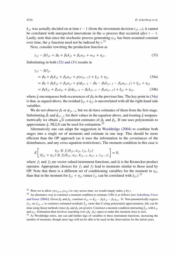
4216 D. Ackerberg et al.
kjt was actually decided on at time t − 1 (from the investment decision ij t−1), it cannotbe correlated with unexpected innovations in the ω process that occurred after t − 1.Lastly, note that since the stochastic process generating ωjt has been assumed constantover time, the g function need not be indexed by t .31
Next, consider rewriting the production function as
(33)yjt − βllj t = β0 + βkkjt + βaajt + ωjt + ηjt .
Substituting in both (32) and (31) results in
yjt − βllj t
(34a)= β0 + βkkjt + βaajt + g(ωjt−1) + ξjt + ηjt
= β0 + βkkjt + βaajt + g(φjt−1 − β0 − βkkjt−1 − βaajt−1) + ξjt + ηjt
(34b)= βkkjt + βaajt + g(φjt−1 − βkkjt−1 − βaajt−1) + ξjt + ηjt ,
where g encompasses both occurrences of β0 in the previous line. The key point in (34a)is that, as argued above, the residual ξjt +ηjt is uncorrelated with all the right-hand sidevariables.
We do not observe βl or φjt−1, but we do have estimates of them from the first stage.Substituting βl and φj t−1 for their values in the equation above, and treating g nonpara-metrically we obtain
√n consistent estimates of βk and βa . If one uses polynomials to
approximate g, NLLS can be used for estimation.32
Alternatively one can adapt the suggestion in Wooldridge (2004) to combine bothstages into a single set of moments and estimate in one step. This should be moreefficient than the OP approach (as it uses the information in the covariances of thedisturbances, and any cross equation restrictions). The moment condition in this case is
E
[ηjt ⊗ f1(kjt , ajt , ij t , lj t )
(ξjt + ηjt ) ⊗ f2(kjt , ajt , kjt−1, ajt−1, ij t−1)
]= 0,
where f1 and f2 are vector valued instrument functions, and ⊗ is the Kronecker productoperator. Appropriate choices for f1 and f2 lead to moments similar to those used byOP. Note that there is a different set of conditioning variables for the moment in ηjt
than that in the moment for ξjt + ηjt (since lj t can be correlated with ξjt ).33
31 Were we to allow p(ωjt+1|ωjt ) to vary across time, we would simply index g by t .32 An alternative way to construct a moment condition to estimate (34b) is as follows [see Ackerberg, Caves
and Fraser (2004)]. Given βk and βa , construct ωj t = φj t − βkkjt − βaajt , ∀t . Non-parametrically regress
ωj t on ωj t−1 to construct estimated residuals ξj t (note that if using polynomial approximation, this can be
done using linear methods (since βk and βa are given)). Construct a moment condition interacting ξj t with kjt
and ajt . Estimation then involves searching over (βk, βa) space to make this moment close to zero.33 As Wooldridge notes, one can add further lags of variables to these instrument functions, increasing thenumber of moments; though more lags will not be able to be used on the observations for the initial years.

Ch. 63: Econometric Tools for Analyzing Market Outcomes 4217
2.3.3. Controlling for endogenous selection
Next we relax the assumption that there is no endogenous exit. Firms now exit accordingto the exit rule given in (26). A first important observation is that the first stage of theOP procedure is not affected by selection. The reason is that by construction, ηjt , theresidual in the first stage equation (30), represents unobservables that are not observed(or predictable) by the firm before input and exit decisions. Thus there is no selectionproblem in estimating (30). Intuitively, the fact that in the first stage we are able tocompletely proxy ωjt means that we can control for both endogenous input choice andendogenous exit.
In contrast, the second stage estimation procedure is affected by endogenous exit.Examining (34b), note that the residual contains not only ηjt , but ξjt . Since the firm’sexit decision in period t depends directly on ωjt (see (26)), the exit decision will becorrelated with ξjt , a component of ωjt .34
We now correct for the selection. Starting from (33), take the expectation of bothsides conditional on both the information at t − 1 and on χjt = 1 (i.e. being in thedataset at t). This results in
E[yjt − βllj t |Ijt−1, χjt = 1]= E[β0 + βkkjt + βaajt + ωjt + ηjt |Ijt−1, χjt = 1]
(35)= β0 + βkkjt + βaajt + E[ωjt |Ijt−1, χjt = 1].The last line follows because: (1) kjt and ajt are known at t − 1, and (2) ηjt is bydefinition uncorrelated with either Ijt−1 or exit at t . Focusing on the last term, wehave
E[ωjt |Ijt−1, χit = 1] = E[ωjt
∣∣Ijt−1, ωjt � ωt(kjt , ajt )]
=∫ ∞
ωt (kjt ,ajt )
ωjt
p(ωjt |ωjt−1)∫∞ωt (kjt ,ajt )
p(ωjt |ωjt−1) dωjt
dωjt
(36)= g(ωjt−1, ωt (kjt , ajt )
).
The first equality follows from the exit rule. The second and third equalities followsfrom the exogenous first order Markov process assumption on the ωjt process.
While we do know ωjt−1 conditional on the parameters (from (31)), we do not di-rectly observe ωt(kjt , ajt ). Modelling ωt(kjt , ajt ) as a nonparametric function of kjt
34 This correlation relies on OP allowing firms to know the realization of ξjt before making the exit decision.Otherwise exit would not cause a selection problem. The longer the time period between observations themore serious the selection problem is likely to be. This point comes out clearly in OP’s comparison of resultsbased on their “balanced” panel (a data set constructed only from the observations of plants that were activethroughout the sample period), to results from their full panel (a panel which keeps the observations on exitingfirms until the year they exit and uses observations on new startups from the year they enter). Selection seemeda far larger problem in the balanced than in the full panel.

4218 D. Ackerberg et al.
and ajt might be a possibility, but this would hinder identification of βk and βa due tocollinearity problems. What we can do is try to control for ωt(kjt , ajt ) using data onobserved exit. Recall that our exit rule is given by
(37)χjt ={
1 (continue)
0 (exit)according as ωjt � ωt(kjt , ajt ).
This means that the probability of being in the data (at period t) conditional on theinformation known at t − 1 is
Pr(χjt = 1|Ijt−1) = Pr(ωjt � ωt(kjt , ajt )
∣∣Ijt−1)
= Pr(χjt = 1
∣∣ωjt−1, ωt (kjt , ajt )) = ˜ϕt
(ωjt−1, ωt (kjt , ajt )
)(38)= ϕt (ωjt−1, kjt , ajt ) = ϕt (ij t−1, kjt−1, ajt−1) = Pjt .
The second to last equality holds because of (28), and the fact that kjt and ajt aredeterministic functions of ij t−1, kjt−1, and ajt−1.
Equation (38) can be estimated nonparametrically, i.e. modelling the probabilityof surviving to t as a nonparametric function of ij t−1, kjt−1, and ajt−1. OP do thisin two alternative ways – first using a probit model with a 4th order polynomial in(ij t−1, kjt−1, ajt−1) as the latent index, second using kernel methods. For a plant char-acterized by (ij t−1, kjt−1, ajt−1), these estimates allow us to generate a consistentestimate of the probability of the plant surviving to period t (Pj t ).
Next, note that as long as the density of ωjt given ωjt−1 is positive in an area aroundωt(kjt , ajt ), (38) can be inverted to write ωt(kjt , ajt ) as a function of ωjt−1 and Pjt ,35
i.e.
(39)ωt(kjt , ajt ) = f (ωjt−1, Pjt ).
Substituting (39) into (36) and (35), and using (31) gives us
E[yjt − βllj t |Ijt−1, χjt = 1] = β0 + βkkjt + βaajt + g(ωjt−1, f (ωjt−1, Pjt )
)= β0 + βkkjt + βaajt + g′(ωjt−1, Pjt )
= β0 + βkkjt + βaajt + g′(φjt−1 − β0
(40)− βkkjt−1 − βaajt−1, Pjt ).
This is similar to (35), only differing in the additional Pjt term in the nonparametricg′ function. Pjt controls for the impact of selection on the expectation of ωjt – i.e. firmswith lower survival probabilities who do in fact survive to t likely have higher ωjt ’s thanthose with higher survival probabilities.
35 Formally, (38) implies that Pjt = ˜ϕt (ωjt−1, ωjt ). With positive density of ωjt around ωjt , ˜ϕt is strictlymonotonic in ωjt , so this can be inverted to generate (39).

Ch. 63: Econometric Tools for Analyzing Market Outcomes 4219
Equation (40) implies that we can write
yjt − βllj t
= β0 + βkkjt + βaajt + g′(φjt−1 − β0 − βkkjt−1 − βaajt−1, Pjt ) + ζjt
(41)= βkkjt + βaajt + g(φjt−1 − βkkjt−1 − βaajt−1, Pjt ) + ζjt + ηjt ,
where, as in (34b), the two β0 terms have been encompassed into the nonparametricfunction g. By construction the residual in this equation satisfies E[ζjt + ηjt |Ijt−1,
χjt = 1] = 0. Substituting Pj t , φj t and βl for Pjt , φjt and βl , (41) can also be estimatedwith NLLS, approximating g with either a polynomial or a kernel.36
In this estimation procedure information on βk and βa is obtained by comparing laborproductivities of firms with the same ωjt−1 and Pjt but different kjt and ajt . In addition,since the functions ϕt (·) and Pt(·) vary across t with changes in industry conditions(while g(·) is assumed constant over time), it also uses information from variation ininputs across firms in different time periods that have the same ωjt−1 and Pjt .
In the selection literature, Pj t is referred to as the propensity score – for discussion ofthese techniques, see, e.g. Heckman (1974, 1978, 1979), Rosenbaum and Rubin (1983),Heckman and Robb (1985), and Ahn and Powell (1993). An important difference be-tween OP and this selection literature is that controlling for the propensity score is notsufficient for OP’s model; they require a control for both ωjt−1 and for ωjt−1.
A number of recent papers have applied the OP procedure successfully. As an ex-ample consider Table 3, which displays the results from the food processing industryin Pavcnik (2002) – this is the first out of the eight industries in her Table 2. Compar-ing the OLS to the OP estimates, we see the changes that we should expect. Returnsto scale decrease (consistent with positive correlation between unobserved productiv-ity and input use), with the coefficients on the more variable inputs accounting for allof the fall (consistent with this correlation being more pronounced for the variable in-puts). Consistent with selection, the capital coefficient rises moving from OLS to OP.The fixed effects estimates are the most difficult to understand, as they generate a co-efficient for capital near zero, and an estimate of economies of scale below 0.9. Theseresults are indicative of those for the other industries in Pavcnik’s Table 2. The aver-age of the returns to scale estimate across industries when estimated by OLS is 1.13,when estimated by OP it is 1.09, and when estimated by fixed effects it is 0.87. Theaverage of the capital coefficients across industries from OLS is 0.066, from OP 0.085,and from fixed effects only 0.021 (with two industries generating negative capital coef-ficients).
OP themselves compare their estimates to estimates obtained using OLS and fixedeffect on both a balanced panel (a panel constructed only from firms that were operatingduring the entire fifteen year sample period) and from the full sample (constructed bykeeping firms that eventually exit until the year prior to their exit and introducing new
36 OP try both the kernel and a polynomial with only minor differences in results.

4220 D. Ackerberg et al.
Table 3Production function estimates from Pavcnik (2002)
OLS Fixed effects Olley–Pakes
Unskilled labor 0.178 0.210 0.153(0.006) (0.010) (0.007)
Skilled labor 0.131 0.029 0.098(0.006) (0.007) (0.009)
Materials 0.763 0.646 0.735(0.004) (0.007) (0.008)
Capital 0.052 0.014 0.079(0.003) (0.006) (0.034)
Source: From Pavcnik (2002).
entrants as they appear). The difference between the balanced sample estimators and OPestimators on the full sample are truly dramatic, and those between the OLS and fixedeffect estimators on the full sample and the OP estimators are similar to those reportedabove (though somewhat larger in absolute value). In both papers, the OP estimatorgenerates standard errors for the labor coefficient that are not too different then thosegenerated by OLS, but, as might be expected, standard errors for the capital coefficientdo increase (though much less so in the OP results than in Pavcnik’s).
2.3.4. Zero investment levels
For simplicity, we assumed above that investment levels for all observations werenonzero. This allowed us to assume that the investment equation was strictly monotonicin ωjt everywhere (and hence could be inverted to recover ωit for every observation).Observations with zero investment call into question the strict monotonicity assumption.However, the OP procedure actually only requires investment to be strictly monotonicin ωjt for a known subset of the data. OP themselves take that subset to be all ob-servations with it > 0, i.e. they simply do not use the observations where investmentequals 0.
Even with this selected sample, first stage estimation of (29) is consistent. Since ωjt
is being completely proxied for, the only unobservable is ηjt , which is by assumptionuncorrelated with labor input and with the selection condition iit > 0. Second stageestimation of (41) is also consistent when OP discard the data where ij t−1 = 0 (φj t−1 −β0 − βkkjt−1 − βaajt−1 is not computable when ij t−1 = 0). The reason is that theerror term in (41) is by construction uncorrelated with the information set Ijt−1, whichcontains the investment level ij t−1. In other words, conditioning on ij t−1 = 0 does notsay anything about the unobservable ζjt .
While the OP procedure can accommodate zero investment levels, this accommo-dation is not without costs. In particular, there is likely to be an efficiency loss fromdiscarding the subset of data where ij t > 0. Levinsohn and Petrin (2003) (henceforth

Ch. 63: Econometric Tools for Analyzing Market Outcomes 4221
LP) suggest an alternative estimation routine whose primary motivation is to eliminatethis efficiency loss. They start by noting that in many datasets, particularly those fromdeveloping countries, the set of observations with zero investment can be quite large.For example, in LP’s dataset on Chilean plants more than 50% of the observations havezero investment (note that in OP’s US plant data, this proportion is much less, ≈8%).To avoid a potentially large efficiency loss, LP suggest using variables other than in-vestment to proxy for the unobserved ωjt . In particular, LP focus on firms’ choices ofintermediate inputs (e.g. electricity, fuels, and/or materials) – these are rarely zero.37
Consider the production function
(42)yjt = β0 + βkkjt + βllj t + βmmjt + ωjt + ηjt
with additional input mjt (e.g. materials). LP assume that like labor, mjt is a variable(i.e. chosen at t), nondynamic input, and consider the following material demand equa-tion
(43)mjt = mt(kjt , ωjt ).
As with the OP investment equation, the demand equation is indexed by t to al-low, e.g. input prices, market structure, and demand conditions to vary across time.38
LP state conditions under which this demand equation is monotonic in ωjt . Given thismonotonicity, estimation proceeds analogously to OP. First, (43) is inverted to give
(44)ωjt = ht (kjt , mjt ).
Next, (44) is substituted into (42) to give
(45)yjt = β0 + βkkjt + βllj t + βmmjt + ht (kjt , mjt ) + ηjt .
Treating the ht function nonparametrically results in the following estimating equa-tion
(46)yjt = βllj t + φt (kjt , mjt ) + ηjt ,
where βk and βm are not separately identified from the nonparametric term. As in OP,the first stage of LP involves estimating (46) to obtain βl and φj t . The second stageof LP again proceeds following OP, the main difference being that the parameter onthe intermediate input, βm, still needs to be estimated. Moving the labor term to the
37 An alternative to LP might be to augment the original OP procedure with a more complete model ofinvestment and/or distributional assumptions on ω, allowing one to utilize the zero investment observations.38 Given that materials are a static choice (in contrast to dynamic investment), one might be more willingto make parametric assumptions on this input demand function (since it depends on fewer primitives, e.g.it does not depend on expectations about the future). However, there are caveats of such an approach, seeSection 2.4.1.

4222 D. Ackerberg et al.
left-hand side and using (32) gives39
(47)yj t = βkkjt + βmmjt + g(φjt−1 − βkkjt−1 − βmmjt−1) + ξjt + ζjt ,
and nonparametric estimates of φjt and of g(·) are used in estimation.Note that since kjt is assumed decided at t − 1, it is orthogonal to the residual,
ξjt + ηjt . However, since mjt is a variable input, it is clearly not orthogonal to ζjt ,the innovation component of ωjt . LP address this by using mjt−1 as an instrument formjt in estimation of (47). In their application LP find biases that are generally consistentwith those predicted by OP, but some differences in actual magnitudes of coefficients.
2.4. Extensions and discussion of OP
The OP model was designed to produce estimates of production function coefficientswhich are not subject to biases due to simultaneity and selection problems generatedby the endogeneity of input demands and exit decisions. We begin this section with atest of whether the coefficient estimates obtained using OP’s assumptions are robust todifferent sources of misspecification.
There are a variety of reasons why this test could fail and the rest of this subsectionconsiders some of the more likely candidates. Each time a source of possible misspeci-fication in OP’s assumption is introduced, we consider modifications to their estimationtechniques which produce consistent estimates of production function coefficients un-der that misspecification. This is in keeping with our belief that different modificationsare likely to be appropriate for different industries and data sets. Though the extendedmodels may well be of more general interest, as they typically will produce richer dy-namics with more detailed policy implications, we limit ourselves to considering theirimplications for estimating production function coefficients.
In this context we first investigate relaxing assumptions on the dynamic implicationsof inputs (e.g. that labor choices today have no dynamic implications) and on the timingof input choices. We then investigate the potential for relaxing the scalar unobservableassumptions of OP. Most of the discussion regarding the timing and dynamic implica-tions of inputs is based on Ackerberg, Caves and Fraser (2004) (ACF) [also see Buettner(2004a) for some related ideas], while much of the discussion on nonscalar unobserv-ables is taken from Ackerberg and Pakes (2005). We also briefly discuss two recentcontributions by Buettner (2004b) and Greenstreet (2005).
2.4.1. A test of Olley and Pakes’ assumptions
This subsection combines results from Section 4.1 in OP with results from ACF. Broadlyspeaking, there are two questionable implications of the assumptions used in OP that
39 While the LP procedure does not formally address selection, they note that their procedure could be ex-tended to control for it in the same way as OP.
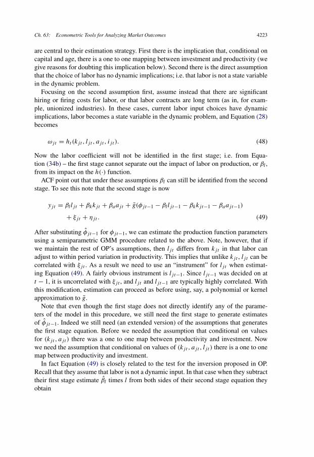
Ch. 63: Econometric Tools for Analyzing Market Outcomes 4223
are central to their estimation strategy. First there is the implication that, conditional oncapital and age, there is a one to one mapping between investment and productivity (wegive reasons for doubting this implication below). Second there is the direct assumptionthat the choice of labor has no dynamic implications; i.e. that labor is not a state variablein the dynamic problem.
Focusing on the second assumption first, assume instead that there are significanthiring or firing costs for labor, or that labor contracts are long term (as in, for exam-ple, unionized industries). In these cases, current labor input choices have dynamicimplications, labor becomes a state variable in the dynamic problem, and Equation (28)becomes
(48)ωjt = ht (kjt , lj t , ajt , ij t ).
Now the labor coefficient will not be identified in the first stage; i.e. from Equa-tion (34b) – the first stage cannot separate out the impact of labor on production, or βl ,from its impact on the h(·) function.
ACF point out that under these assumptions βl can still be identified from the secondstage. To see this note that the second stage is now
yjt = βllj t + βkkjt + βaajt + g(φjt−1 − βllj t−1 − βkkjt−1 − βaajt−1)
(49)+ ξjt + ηjt .
After substituting φj t−1 for φjt−1, we can estimate the production function parametersusing a semiparametric GMM procedure related to the above. Note, however, that ifwe maintain the rest of OP’s assumptions, then lj t differs from kjt in that labor canadjust to within period variation in productivity. This implies that unlike kjt , lj t can becorrelated with ξjt . As a result we need to use an “instrument” for lj t when estimat-ing Equation (49). A fairly obvious instrument is lj t−1. Since lj t−1 was decided on att − 1, it is uncorrelated with ξjt , and lj t and lj t−1 are typically highly correlated. Withthis modification, estimation can proceed as before using, say, a polynomial or kernelapproximation to g.
Note that even though the first stage does not directly identify any of the parame-ters of the model in this procedure, we still need the first stage to generate estimatesof φj t−1. Indeed we still need (an extended version) of the assumptions that generatesthe first stage equation. Before we needed the assumption that conditional on valuesfor (kjt , ajt ) there was a one to one map between productivity and investment. Nowwe need the assumption that conditional on values of (kjt , ajt , lj t ) there is a one to onemap between productivity and investment.
In fact Equation (49) is closely related to the test for the inversion proposed in OP.Recall that they assume that labor is not a dynamic input. In that case when they subtracttheir first stage estimate βl times l from both sides of their second stage equation theyobtain

4224 D. Ackerberg et al.
yjt − βl lj t = (βl − βl)lj t + βkkjt + βaajt + g(φj t−1 − βkkjt−1 − βaajt−1)
(50)+ ξjt + ηjt ,
which is an equation with over identifying restrictions.40
In particular, the term (βl − βl)lj t in Equation (50) should be zero if the inversionwhich leads to the estimate of the labor coefficient is a good approximation to reality.Further the inversion implies that what we must subtract from our estimate of φjt−1 toobtain lagged productivity is determined by the contribution of (kjt−1, ajt−1) to pro-duction of yjt−1, i.e. by (βk, βa). These coefficients also determine the contribution of(kjt , ajt ) to yjt given ωjt−1. If our inversion were seriously in error we would expectthat φjt−1 − βkkjt−1 − βaajt−1 would not be perfectly correlated with ωjt−1 and as aresult there would be a residual component of productivity we are not controlling for.Provided there was an endogeneity problem in the first place, this residual should becorrelated with (kjt , ajt ). Thus OP allow the coefficients on (kjt , ajt ) to differ fromthose on (kjt−1, ajt−1) in Equation (50), use (lj,t−1, kjt , ajt ) and powers and lags ofthese variables as instruments, and then test whether βl − βl = 0, and whether thecoefficients on the current and lagged values of k and a are equal.41
As noted previously, when the current labor choice has dynamic implications the firststage estimate of βl obtained by OP is inconsistent (regardless of whether the inversionis correct). However even if labor is dynamic, Equation (49) still generates over iden-tifying restrictions; the existence of the inversion implies that the current and laggedvalues of (l, k, a) should enter in this equation with the same factors of proportion-ality. In other words, if the inversion is correct then what we must subtract from ourestimate of φjt−1 to obtain lagged productivity is determined by the contribution of(lj t−1, kjt−1, ajt−1) to production of yjt−1, i.e. by (βl, βk, βa). These coefficients alsodetermine the contribution of (lj t , kjt , ajt ) to yjt given ωjt−1. That is if we were toestimate
yjt = β∗l lj t + β∗
k kjt + β∗a ajt + g(φjt−1 − βllj t−1 − βkkjt−1 − βaajt−1)
(51)+ ξjt + ηjt ,
and then test whether (β∗l , β∗
k , β∗a ) = (βk, βl, βa), with a large enough data set we
should reject the null of equality if assumptions which underlie the inversion are wrong.Given the additional parameters one will need additional instruments to estimate thisspecification. Natural instruments would be those used in OP, i.e. (lj,t−1, kjt , ajt ) andpowers and lags of these variables.
Two other points about the test. First, the OP test conditions on the fact that laboris variable (i.e. it is not a state variable) and endogenous (current labor is correlated
40 We have omitted a term that results from substituting φj t−1 for the true φjt−1 in this equation. The addi-
tional term’s impact on the parameter estimates is op(1/√
J ), and so does not effect their limit distributions.41 Note that we cannot use both current and lagged values of ajt as instruments for the two are collinear. Wecould, however, use different functions of ajt as additional instruments.

Ch. 63: Econometric Tools for Analyzing Market Outcomes 4225
with ξjt ), and then tests whether the inversion is a good approximation. We could havealternatively proceeded by conditioning on the inversion and then tested one or bothof the assumptions that; labor is dynamic and/or labor choices are fixed prior to therealization of ξt . We would do this by estimating both stages of ACF simultaneouslyand then testing constraints. The constraint to be tested in asking whether labor can betreated as a nondynamic (or variable) input is whether φ(ljt , ij t , kjt , ajt ) = βllj t +φ(ijt , kjt , ajt ). To test whether labor is endogenous (in the sense that it can react to ξjt )we estimate the system once using lj t−1 as an instrument for lj t in Equation (49) andonce using lj t as an instrument for itself. Exactly what it makes sense to condition on(and what to test for) is likely to depend on the characteristics of the industry beingstudied. Alternatively we could improve the power of the omnibus test in Equation (49)by estimating the first stage in ACF simultaneously with this equation and then askingwhether (β∗
l , β∗k , β∗
a ) = (βl, βk, βa). If that is accepted we could then test the additional(nested) constraints implied by an assumption that labor is not endogeous.42
Finally a word of caution on the usefulness of these tests. First we have made noattempt to look at the power of these tests. Though OP find very precise estimates ofdifferences in coefficients from (51), their data seems to deliver more precise estimatesthan many other data sets (see, for e.g. ACF). Second it is important to realize that thetest that (β∗
l , β∗k , β∗
a ) = (βl, βk, βa) is designed to ask the limited question of whethermaking our approximations greatly hinders our ability to obtain reasonable produc-tion function coefficients. As a result we are using the difference in these coefficients,normalized by the variance-covariance of those differences, as our metric for “reason-ableness”. There are other metrics possible, one of which would be to have some priorknowledge of the characteristics of the industry the researcher is working on (and weexpect these results to vary by industry). Further there may well be independent rea-sons for interest in the timing of input decisions or in our invertibility assumption (seethe discussion below), and a test result that our approximations do not do terrible harmto production function estimates does not imply that they would do little harm in theanalysis of other issues (for example in the analysis of the response of labor hiring to achange in demand, or in the response of investment to an infrastructure change whichincreases productivity).
42 Note that both these ideas: that one can allow labor to have dynamic effects and that some of the as-sumptions behind these procedures are testable – are related to the dynamic panel literature cited above [e.g.Arellano and Bond (1991), Arellano and Bover (1995), and Blundell and Bond (1999)] in that further lagsof inputs are typically used as instruments. If one were willing to assume that the ηj,t are independentlydistributed across time then the residuals should be uncorrelated with past values of output also. However ifηjt represented serially correlated measurement error in the observations on yt then the ηjt may be seriallycorrelated, and we could not expect a zero correlation between past output and the disturbance from (51).ACF flesh out the distinction between their methods and the dynamic panel literature further.

4226 D. Ackerberg et al.
2.4.2. Relaxing assumptions on inputs
This subsection assumes that there is an inversion from productivity to investment con-ditional on the state variables of the problem, and investigates questions regarding thenature of the input demands given this inversion. ACF note that there are two dimen-sions along which we can classify inputs in this context, and the two dimensions havedifferent implications for the properties of alternative estimators. First inputs can eitherbe variable (correlated with ξjt ) or fixed (uncorrelated with ξjt ). Second the inputs caneither be dynamic, i.e. be state variables in the dynamic problem and hence conditionedon in the relationship between productivity and investment, or static. So if we general-ize, and allow for inputs of each of the four implicit types we have
(52)yjt = βvsXvsj t + βvdXvd
j t + βfsXfsj t + βfdXfd
j t + ωjt + ηjt ,
where the input acronyms correspond to these dimensions, e.g. Xvsj t represent variable,
nondynamic inputs, while Xfdj t represent fixed, dynamic inputs, and so on.
The various coefficients can be identified in different ways. βvs, like labor in theoriginal OP framework, can be identified either in the first stage, or in the second stageusing Xvs
j t−1 as an instrument (because Xvsj t is variable and thus potentially correlated
with ξjt , it cannot be used as an instrument in the second stage). βfd, like capital in theoriginal OP framework, cannot be identified in the first stage, but it can be identified inthe second stage using either Xfd
j t or Xfdj t−1 (or both) as instruments. βvd, the coefficients
on the inputs that are variable and dynamic, also cannot be identified in the first stage,but can be identified in the second stage using Xvd
j t−1 as an instrument. Lastly, βfs can
be identified either in the first stage or in the second stage using either Xfsj t or Xfs
j t−1 (orboth) as instruments.
Note also that if we have any static or fixed inputs we have over identifying restric-tions.43 This over identification can potentially be useful in testing some of the timingassumptions. For example, suppose one starts by treating capital as a fixed, dynamicinput. One could then estimate the second stage using both kit−1 and kit as instruments,an over identified model. In the GMM context, one could test this over identificationwith a J-test [Hansen (1982)]. Since kit is a valid instrument only when capital is trulyfixed (yet kit−1 is a valid instrument regardless) rejection of the specification might beinterpreted as evidence that capital is not a completely fixed input. Consistent estima-tion could then proceed using only kit−1 as an instrument. Again, the Wooldridge (2004)framework makes combining these multiple sources of identification and/or testing veryconvenient.
ACF also look deeper into the various assumptions on inputs. They note that, underthe assumption that lj t is a variable input, for it to have the independent variance needed
43 In all these cases, further lags (prior to t − 1) of the inputs can be used as instruments and thus as overidentifying restrictions, although it is not clear how much extra information is in these additional momentconditions, and one will not be able to use these additional lags in the initial time periods.

Ch. 63: Econometric Tools for Analyzing Market Outcomes 4227
to estimate our first stage equation (30), there must be a variable, say zjt , that impactsfirms’ choices of lj t but that does not impact choices of investment at t . This variablezjt must also have some variance that is independent of ωjt and kjt . If this were notthe case, e.g. if lj t = ft (ωjt , kjt ), then one can show that lj t is perfectly collinearwith the nonparametric function in Equation (30), implying that one cannot estimateβl from that equation. Note that the variable zjt does not need to be observed by theeconometrician.
Thus, to proceed as OP do we need the demand function for labor to be
lj t = ft (ωjt , kjt , zjt ),
where zjt are additional factors that affect demand for labor (or more generally, demandfor the variable inputs) with nonzero conditional variance (conditional on ωjt , kjt ). Notethat the zjt cannot be serially correlated. If this were the case, then zjt would becomepart of the state space, influence ij t , and one would not be able to do the inversion.44
Even with this restriction, there are at least two possible zjt ’s here: i.i.d. firm specificinput price shocks and i.i.d. random draws to the environment that cause differencesin the variance of ηjt over time (since the profit function is a convex function of η
the variance in this variable will affect labor demand). The latter could be associatedwith upcoming union negotiations, the likelihood of machine break downs due to age ofequipment, or the approach of maintenance periods. One problem with the i.i.d. inputprice shock story is that it is somewhat at odds with the assumptions that all othercomponents of prices are constant across firms and that the other unobservables (ωjt )in the model are serially correlated over time.
ACF provide two additional ways of overcoming this problem. First they note that ifone weakens OP’s timing assumptions slightly, one can still identify lj t in the first stage.Their observation also reopens an avenue of research on the timing of input decisionswhich dates back at least to Nadiri and Rosen (1974). Suppose that lj t is actually not aperfectly variable input, and is chosen at some point in time between period t − 1 andperiod t . Denote this point in time as t − b, where 0 < b < 1. Suppose that ω evolvesbetween the subperiods t − 1, t − b, and t according to a first order Markov process, i.e.
p(ωjt |Ijt−b) = p(ωjt |ωjt−b) and p(ωjt−b|Ijt−1) = p(ωjt−b|ωjt−1).
In this case, labor input is not a function of ωjt , but of ωjt−b, i.e.
lj t = ft (ωjt−b, kjt ).
Since ωjt−b cannot generally be written as a function of kjt , ajt , and ij t , lj t will notgenerally be collinear with the nonparametric term in (30), allowing the equation tobe identified. The movement of ω between t − b and t is what breaks the collinearityproblem between lj t and the nonparametric function. The second alternative suggested
44 Note also that observing zjt would not help in this serially correlated case. While one would now be ableto do the inversion, zjt would enter the nonparametric function, again generating perfect collinearity.

4228 D. Ackerberg et al.
by ACF avoids this collinearity problem by abandoning the first stage identification ofthe labor coefficient. Instead, they suggest identifying the labor coefficient in the secondstage using lj t−1 as an instrument.
Importantly, ACF argue that this collinearity problem is more severe when using theLP procedure. They contend that it is considerably harder to tell a believable story inwhich the assumptions of LP hold and where lj t varies independently of the nonpara-metric function in (46). The reason for this is that it is hard to think of a variable zjt
that would affect a firms’ labor choices but not their material input choices (either di-rectly or indirectly through the labor choice).45 ACF suggest a couple of proceduresas alternatives to LP.46 The first, based on the discussion above, again involves simplyidentifying the labor coefficient in the second stage. This can be done using either lj t
or lj t−1 to form an orthogonality condition, depending on what one wants to assumeabout the timing of the labor choice. Moreover, it can also be done in a manner that isalso consistent with labor having dynamic effects. The second procedure is more com-plicated and involves sequentially inverting the value of ωjt at each point in time atwhich inputs are chosen. While this procedure depends on independence (rather thanmean independence) assumptions on innovations in ωjt , it has the added advantage ofallowing one to infer something about the point in time that labor is chosen. Bond andSöderbom (2005) make a somewhat related point regarding collinearity. They argue thatin a Cobb–Douglas context where input prices are constant across firms, it is hard if notimpossible to identify coefficients on inputs that are perfectly variable and have no dy-namic effects. This is important for thinking about identification of coefficients on Xvs
j t
in the above formulation.
2.4.3. Relaxing the scalar unobservable assumption
The assumption of a scalar unobserved state variable is another aspect of the OP ap-proach that might be a source of concern. We begin with three reasons for worryingabout this assumption and then provide a way of modifying the model to account foreach of them. In each case we bring information on additional observables to bear onthe problem. As a result, one way of looking at this section is as a set of robustness testsconducted by asking whether the additional observables affect the results.
Our three concerns in order of increasing difficulty are as follows. First productivityitself is a complex functions of many factors, and it may not be appropriate to assume
45 ACF note that one probably will not observe this perfect collinearity problem in practice (in the sensethat the first stage procedure will actually produce an “estimate”). However, they point out that unless oneis willing to make what they argue are extremely strong and unintuitive assumptions, the lack of perfectcollinearity in practice must come from misspecification in the LP model.46 An alternative approach to dealing with these collinearity problems might be to model the input demandfunctions (investment or materials) parametrically. If g( ) is parametric, one does not necessarily have thiscollinearity problem. However, at least in the LP situation this does not guarantee identification. ACF showthat in the Cobb–Douglas case, substituting in the implied parametric version of the material input functionleads to an equation that cannot identify the labor coefficient.

Ch. 63: Econometric Tools for Analyzing Market Outcomes 4229
that one can represent it as a first order Markov process. Second investment might wellrespond to demand factors that are independent of the firm’s productivity. Then there isno longer a one to one mapping between investment and productivity given capital andage. Consequently we cannot do the inversion in Equation (28) underlying the first stageof the OP procedure. Finally, at least in some industries we often think of two sourcesof increments in productivity, one that results from the firm’s own research investments,and one whose increments do not depend on the firm’s behavior. A process formedfrom the sum of two different first order Markov processes is not generally a first orderMarkov process, and if one of those processes is “controlled” it may well be difficult toaccount for it in the same way as we can control for exogenous Markov processes.
First assume that productivity follows a second order (rather than first order) Markovprocess. This changes the investment demand equation to
(53)ij t = it (kjt , ajt , ωjt , ωjt−1).
Since there are the two unobservables (ωjt , ωjt−1) the investment equation cannot beinverted to obtain ωjt as a function of observables, and the argument underlying the firststage of the OP process is no longer valid.
One possible solution to the estimation problem is through a second observed controlof the firm. Suppose, for example, one observes firms’ expenditures on another invest-ment (advertising, expenditure on a distributor or repair network), say sit .47 Then wehave the bivariate policy function(
ij t
sj t
)= Υt(kjt , ajt , ωjt , ωjt−1).
If the bivariate function Υt ≡ (Υ1,t , Υ2,t ) is a bijection in (ωjt , ωjt−1) (i.e. it is onto),then it can be inverted in ωjt to obtain
ωjt = Υ −1t (kjt , ajt , ij t , sj t ).
Given this assumption the first stage proceeds as in OP, except with a higher dimensionalnonparametric function to account for current productivity (it is a function of sjt as wellas (kjt , ajt , ij t )).
OP’s second stage is modified to be
yj t = βkkjt + βaajt
+ g(φj t−1 − βkkjt−1 − βaajt−1, φj t−2 − βkkjt−2 − βaajt−2)
+ ξjt + ηjt ,
where yj t = yjt − βlj t and the φj t variables are obtained from the first stage estimatesat t − 1 and t − 2. Note that since the conditional expectation of ωjt given Ijt−1 now
47 One can modify this argument to allow also for a second state variable, the stock of advertising or the sizeof the repair network, provided that stock is known up to a parameter to be estimated.

4230 D. Ackerberg et al.
depends on ωjt−2 as well as ωjt−1, we need to use estimates of φ from two prior periods.The extension to control for selection as well is straightforward. Moreover, provided thenumber of observed control variables is at least equal to the order of the Markov process,higher order Markov processes can be handled in the same way.
We now move on to allow investment to depend on an unobservable demand shockthat varies across firms, in addition to the (now first order) ωjt process. Suppose thatthe demand shock, μjt , also follows a first order Markov process that is independent ofthe ωjt process. Then the investment function will be a function of both unobservables,or ij t = it (kjt , ajt , ωjt , μjt ). Again we will assume the existence of a second controland use it to allow us to substitute for ωjt in the first stage of OP’s procedure.
More precisely, assume we also observe the firms’ pricing decisions pjt . At the risk ofsome notational confusion, again let the bivariate policy function determining (ij t , pjt )
be labelled Υ (·), and assume it is a bijection in (ωjt , μjt ) conditional on (kjt , ajt ).Then it can be inverted to form
(54)ωjt = Υ −1t (kjt , ajt , ij t , pjt )
and one can proceed with the first stage of estimation as above.For the second stage observe that since the μjt process is independent of the ωjt
process the firm’s conditional expectation of ωjt given Ijt−1 only depends on ωjt−1.Thus, the second stage is
(55)yj t = βkkjt + βaajt + g(φj t−1 − βkkjt−1 − βaajt−1) + ξjt + ηjt .
Note that the demand shock, if an important determinant of ij t , may help with theprecision of our estimates, as it generates independent variance in φ.
The estimation problem becomes more complicated if, for some reason, the twoMarkov processes are dependent. The problem is that in this case, the firm’s conditionalexpectation of ωjt given Ijt−1 depends on both ωjt−1 and μjt−1. Then Equation (55)will have to be amended to allow g(·) to also depend on μjt−1. If we let
(56)μjt−1 = Υ −12,t−1(kjt−1, ajt−1, ij t−1, pjt−1),
our second stage can then be written as
yj t = βkkjt + βaajt + g(ωjt−1, μjt−1) + ξjt + ηjt
= βkkjt + βaajt
+ g(φjt−1 − βkkjt−1 − βaajt−1, Υ
−12,t−1(kjt−1, ajt−1, ij t−1, pjt−1)
)(57)+ ξjt + ηjt .
Unfortunately, this equation cannot identify βk and βa since it requires us to condi-tion on a nonparametric function of (kjt−1, ij t−1, ajt−1). More formally, since kjt =(1 − δ)kjt−1 + ij t−1 (and ajt = ajt−1 + 1), there is no remaining independent variancein (kjt , ajt ) to be used to identify βk and βa .

Ch. 63: Econometric Tools for Analyzing Market Outcomes 4231
To avoid this problem, we need an explicit ability to solve for or estimate μjt−1.This would generally require demand side data. For example, the Berry, Levinsohn andPakes (1995) demand estimation procedure produces estimates of a set of “unobservedproduct characteristics” which might be used as the μjt ’s. Of course, once one bringsin the demand side, there is other information that can often be brought to bear onthe problem. For example, the production function estimates should imply estimates ofmarginal cost which, together with the demand system, would actually determine pricesin a “static” Nash pricing equilibrium (see the first section of this chapter). We do notpursue this further here.
Finally we move to the case where there are two sources of productivity growth, oneevolving as a controlled Markov process, and one as an exogenous Markov process. Inthis case the production function is written as
yjt = β0 + βkkjt + βaajt + βllj t + ω1j t + ω2
j t + ηjt ,
where ω1j t is the controlled, and ω2
j t is the exogenous, first order Markov process.Assume now that we have data on both R&D expenditures, say rt , which is the input
of the controlled process, and a “technology indicator” or Tt (like patents, or licensingfees) which is an output of the controlled process. As above, assume the policy functionsfor physical and R&D investment are a bijection, so we can write
ω1j t = Υ −1
1t (kjt , ajt , ij t , rj t ),
(58)ω2j t = Υ −1
2t (kjt , ajt , ij t , rj t ).
Now the first stage consists of using the technology indicator to isolate ω1j t . In other
words, we assume
(59)Tjt = ω1j t θ + η2j t ,
where η2,t is mean independent of all the controls. We then substitute a nonparametricfunction of (kjt , ajt , ij t , rj t ) for ω1
j t in Equation (59). This provides us with an estimate
of ω1j t θ , say Υ −1
1tj .
Our second stage mimics the first stage of OP except we treat Υ −11tj as an input. That
is, we estimate
(60)yjt = βllj t + φ(kjt , ajt , ij t , rj t ) + ηjt ,
where
φ(kjt , ajt , ij t , rj t ) = βkkjt + βaajt + θ−1Υ −11j t + ω2
j t .
Then, without a selection correction, the third stage becomes
yj t = βkkjt + βaajt + g(φjt−1 − βkkjt−1 − βaajt−1, Υ
−11j t−1
)+ ξjt + ηjt .
Once again, we can modify this to allow for selection by using the propensity score asan additional determinant of g(·).

4232 D. Ackerberg et al.
Buettner (2004b) explores a related extension to OP. While he only allows one un-observed state variable, he does allow the distribution of ωjt to evolve endogenouslyover time, i.e. firms invest in R&D and these investments affect the distribution of ωjt
(conditional on ωjt−1).48 Unlike the above, Buettner does not assume that a “technol-ogy indicator” is observed. He develops a dynamic model with investments in R&D andphysical capital that generates invertible policy functions such that the first stage of OPcan be directly applied (and the labor coefficient can be estimated). However, secondstage estimation is problematic, since the conditional expectation of ωjt now dependson the full state vector through the choice of R&D. Furthermore, with the endogenousproductivity process, he cannot rely on exogenous variation (such as changes in theeconomic environment over time) for identification. It remains to be seen whether thisproblem can be solved.
Greenstreet (2005) proposes and utilizes an alternative model/methodology that,while related to the above procedures, does not require the first stage inversion. This isa very nice attribute since as a result, the procedure does not rely at all on the key scalarunobservable and monotonicity assumptions of the OP/LP/ACF procedures. Greenstreetachieves this by making a different assumption on firms’ information sets. Specifically,instead of observing ωjt and ηjt individually (after production at t), firms only everobserve the sum ωjt + ηjt . Because of this alternative informational assumption, theeconometrician does not need the first-stage inversion to recreate the information set ofthe firms. While this does avoid the scalar unobservable and monotonicity assumptions,Greenstreet’s approach still relies on similar timing assumptions, involves a slightlymore complicated learning process than the above procedures (requiring Kalman filter-ing), and also generates some new initial conditions problems that require additionalassumptions to solve.
2.5. Concluding remark
The increase in the availability of plant and/or firm level panels together with a desireto understand the efficiency implications of major environmental and policy changeshas led to a renewed interest in productivity analysis. Most of this analysis is basedon production function estimates, and the literature has found at least two empiricalregularities. First, there are indeed large efficiency differences among firms and thosedifferences are highly serially correlated. Second, at least in many environments, toobtain realistic production function estimates the researcher must account for the possi-bility of simultaneity and selection biases.
Put differently, to study either the changes in the allocative efficiency of productionamong firms of differing productivities, or the correlates of productivity growth withinindividual establishments, we first have to isolate the productivity variable itself. Sincefirms’ responses to the changes in the environment being studied typically depend on
48 Recall that “endogenous” evolution of ωjt is problematic for IV approaches.

Ch. 63: Econometric Tools for Analyzing Market Outcomes 4233
how those changes impacted their productivity, movements in productivity cannot beisolated from changes in input and exit choices without an explicit model of how thosechoices are made.
The appropriateness of different models of how these decisions are made will un-doubtedly depend on the environment being studied. We have presented a number ofalternatives, and discussed their properties. However this is an empirically driven sub-field of estimation, and there are undoubtedly institutional settings where alternativeframeworks might be better to use. It is not the precise framework that is important,but rather the fact that productivity studies must take explicit account of the fact thatchanges in productivity (or, if one prefers, sales for a given amount of inputs) in largepart determine how firms respond to the changes being studied, and these must be takeninto account in the estimation procedure.
3. Dynamic estimation
This chapter considers structural estimation of dynamic games. Despite a blossomingempirical literature on structural estimation of static equilibrium models, there has beenrelatively little empirical work to date on estimation of dynamic oligopoly problems.Four exceptions are Gowrisankaran and Town (1997), Benkard (2004), Jofre-Bonet andPesendorfer (2003), and Ryan (2006). The literature’s focus on static settings cameabout not because dynamics were thought to be unimportant to market outcomes, butrather because empirical analysis of dynamic games was seen as too difficult. In particu-lar, while some of the parameters needed to analyze dynamic games could be estimatedwithout imposing the dynamic equilibrium conditions, some could not and, until veryrecently, the only available methods for estimating these remaining parameters wereextremely burdensome, in terms of both computation time and researcher time.
This computational complexity resulted from the need to compute the continuationvalues to the dynamic game in order to estimate the model. The direct way of obtainingcontinuation values was to compute them as the fixed point to a functional equation,a high order computational problem. Parameter values were inferred from observed be-havior by computing the fixed point that determines continuation values at different trialparameter values, and then searching for the parameter value that makes the behaviorimplied by the continuation values “as close as possible” to the observed behavior. This“nested fixed point” algorithm is extremely computationally burdensome because thecontinuation values need to be computed many times.
However, a recent literature in industrial organization [Aguirregabiria and Mira(2007), Bajari, Benkard and Levin (2007), Jofre-Bonet and Pesendorfer (2003), Pakes,Ostrovsky and Berry (2007), and Pesendorfer and Schmidt-Dengler (2003)] has devel-oped techniques that substantially reduce the computational and programming burdensof estimating dynamic games. This literature extends a basic idea that first appeared inthe context of single agent problems in Hotz and Miller (1993). Hotz and Miller (1993)provided a set of assumptions under which one could obtain a nonparametric estimate

4234 D. Ackerberg et al.
of continuation values without ever computing the fixed point.49 Rust (1994) suggeststhe extension of these ideas to the context of dynamic games. The recent literature inindustrial organization has shown that, at least under a certain set of assumptions, theseapproaches can be extended to estimate continuation values in a wide variety of dynamicgames, even in the presence of multiple equilibria.
This chapter summarizes the currently available techniques for estimating dynamicgames, concentrating on this recent literature. The chapter proceeds as follows. We firstoutline the goals of the estimation procedure and consider what might be gained bymodelling dynamics in an oligopoly situation. Then we present a general frameworkfor dynamic oligopoly problems, with three simple examples from the recent literature.Next we overview existing estimation methods, providing details for the three examples.We conclude with a brief discussion of techniques available to ameliorate one (of many)outstanding problems; that of serially correlated unobserved state variables.
We note that there are at least two issues that appear in the literature and are notconsidered here. First we do not consider identification issues (at least not directly).Our feeling is that many of the parameters determining behavior in dynamic games canbe estimated without ever computing an equilibrium, and those parameters that remaindepend on the nature of the problem and data availability. Second, we do not consider“timing” games, such as those in Einav (2003) and in Schmidt-Dengler (2003). Ouronly excuse here is our focus on the evolution of market structure in oligopolies.
3.1. Why are we interested?
One contribution of the recent literature is that it provides a means of obtaining informa-tion about certain parameters that could not be obtained via other methods. For example,the sunk costs of entry and the sell-off values (or costs) associated with exit are key de-terminants in the dynamics of market adjustments to policy and environmental changes.Knowledge of the level of sunk costs is critical, for example, in a regulatory author-ity’s decision of whether to approve a merger, or in the analysis of the likely impactsof changes in pension policy on shut down decisions. However, actual data on sunkcosts are extremely rare. Besides being proprietary, and thus hard to access, sunk costscan also be very difficult to measure. Thus, in many cases the only option for learningthe extent of sunk costs may be to infer them from equilibrium behavior using othervariables that we can observe. Since sunk costs are only paid once upon entry, whilefirms may continue to operate for many periods, inferring the level of sunk costs fromequilibrium behavior requires a dynamic framework. Similar arguments can be maderegarding the parameters determining, among other diverse phenomena, the transaction
49 In related work Olley and Pakes (1996) use nonparametrics to get around the problem of computing thefixed point needed to obtain an agent’s decision rule in a multiple agent framework; but they use the non-parametric estimates to control for unobservables and do not recover the implied estimates of continuationvalues.

Ch. 63: Econometric Tools for Analyzing Market Outcomes 4235
costs of investments (including installment, delivery, and ordering costs), the costs ofadjusting output rates or production mix, and the extent of learning-by-doing.
There are a number of other uses for techniques that enable us to empirically analyzedynamic games. For example, there are many industries in which an understanding ofthe nature of competition in prices (or quantities) requires a dynamic framework. In suchcases, the empirical literature in industrial organization has often used static models toapproximate behavior that the authors are well aware is inherently dynamic. For exam-ple, there has been much work on identifying and estimating the form of competition inmarkets [e.g. Bresnahan (1982, 1987), Lau (1982)]. This literature typically compares astatic Nash equilibrium with particular static “collusive” pricing schemes. In reality, theset of collusive pricing schemes that could be supported in equilibrium depends on thenature of the dynamic interactions [e.g. Abreu, Pearce and Stacchetti (1986), Green andPorter (1984), Rotemberg and Saloner (1985), Fershtman and Pakes (2000)]. A relatedpoint is that static price or quantity setting models are known to be inappropriate whenfuture costs depend directly on the quantity sold today, as in models with learning bydoing or adjustment costs, and/or when future demand conditions depend on currentquantities sold, as in models with durable goods, experience goods, the ability to holdinventory, and network externalities.
Similarly, most of the existing empirical literature on entry relies on two-period sta-tic models. While these models have proven very useful in organizing empirical facts,the two period game framework used makes little sense unless sunk costs are absent.Therefore, the results are not likely to be useful for the analysis of policy or envi-ronmental changes in a given market over time. This leaves us with an inability toanalyze the dynamic implications of a host of policy issues, and there are many sit-uations where dynamics may substantially alter the desirability of different policies.For example, Fershtman and Pakes (2000) show that because collusive behavior canhelp promote entry and investment, it can enhance consumer welfare. Similarly, a sta-tic analysis would typically suggest that mergers lower consumer welfare by increasingconcentration, whereas a dynamic analysis might show that allowing mergers promotesentry, counterbalancing the static effects.
3.2. Framework
This section outlines a framework for dynamic competition between oligopolistic com-petitors that encompasses many (but not all) applications in industrial organization.Examples that fit into the general framework include entry and exit decisions, dynamicpricing (network effects, learning-by-doing, or durable goods), dynamic auction games,collusion, and investments in capital stock, advertising, or research and development.The defining feature of the framework is that actions taken in a given period affect futurepayoffs, and future strategic interaction, by influencing only a set of commonly observedstate variables. In particular, we will assume that all agents have the same informationto use in making their decisions, up to a set of disturbances that have only transitoryeffects on payoffs.

4236 D. Ackerberg et al.
We use a discrete time infinite horizon model, so time is indexed by t = 1, 2, . . . ,∞.At time t , prevailing conditions are summarized by a state, st ∈ S ⊂ R
G, that reflectsaspects of the world relevant to the payoffs of the agents. Relevant state variables mightinclude firms’ production capacities, the characteristics of the products they produce,their technological progress up to time t , the current market shares, stocks of consumerloyalty, or simply the set of firms that are incumbent in the market. We assume that thesestate variables are commonly observed by the firms. Note that we have not yet specifiedwhich state variables are observed by the econometrician. This distinction will be madein the applications below.
Given the state st at date t , the firms simultaneously choose actions. Depending onthe application, the firms’ actions could include decisions about whether to enter or exitthe market, investment or advertising levels, or choices about prices and quantities. Letait ∈ Ai denote firm i’s action at date t , and at = (a1t , . . . , aNt ) the vector of time t
actions, where Nt is the number of incumbents in period t (entry and exit, and hence Nt ,are endogenous in these models).
We also assume that before choosing its action each firm, i, observes a private shockνit ∈ R, drawn independently (both over time and across agents) from a distributionG(·|st ).50 Private information might derive from variability in marginal costs of produc-tion that result, say, from machine breakdowns, or from the need for plant maintenance,or from variability in sunk costs of entry or exit. We let the vector of private shocks beνt = (ν1t , . . . , νNt ).
In each period, each firm earns profits equal to πi(at , st , νit ). Profits might includevariable profits as well as any fixed or sunk costs, including the sunk cost of entryand the selloff value of the firm. Conditional on the current state, s0, and the currentvalue of the firm’s private shock, νi0, each firm is interested in maximizing its expecteddiscounted sum of profits
(61)E
[ ∞∑t=0
βtπi(at , st , νit )
∣∣∣∣s0, νi0
],
where the expectation is taken over rival firms’ actions in the current period as well asthe future values of all state variables, the future values of the private shock, and allrivals’ future actions. We assume firms have a common discount factor β.
The final aspect of the model is to specify the transitions between states. We as-sume that the state at date t + 1, denoted st+1, is drawn from a probability distributionP(st+1|st , at ). The dependence of P(·|st , at ) on the current period actions at reflectsthe fact that some time t decisions may affect future payoffs, as is clearly the case if therelevant decision being modelled is an entry/exit decision or a long-term investment.Of course, not all the state variables necessarily depend on past actions; for example,
50 Here we assume that firm i’s private shock is a single scalar variable. However, as will be seen in theexamples below, there is no conceptual difficulty in allowing the shock to be multi-dimensional.
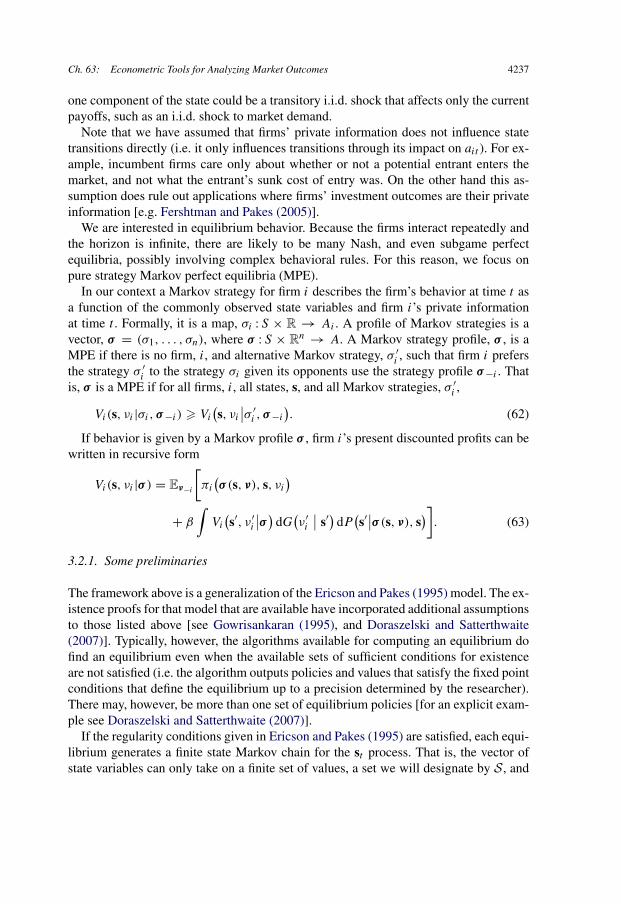
Ch. 63: Econometric Tools for Analyzing Market Outcomes 4237
one component of the state could be a transitory i.i.d. shock that affects only the currentpayoffs, such as an i.i.d. shock to market demand.
Note that we have assumed that firms’ private information does not influence statetransitions directly (i.e. it only influences transitions through its impact on ait ). For ex-ample, incumbent firms care only about whether or not a potential entrant enters themarket, and not what the entrant’s sunk cost of entry was. On the other hand this as-sumption does rule out applications where firms’ investment outcomes are their privateinformation [e.g. Fershtman and Pakes (2005)].
We are interested in equilibrium behavior. Because the firms interact repeatedly andthe horizon is infinite, there are likely to be many Nash, and even subgame perfectequilibria, possibly involving complex behavioral rules. For this reason, we focus onpure strategy Markov perfect equilibria (MPE).
In our context a Markov strategy for firm i describes the firm’s behavior at time t asa function of the commonly observed state variables and firm i’s private informationat time t . Formally, it is a map, σi : S × R → Ai . A profile of Markov strategies is avector, σ = (σ1, . . . , σn), where σ : S × R
n → A. A Markov strategy profile, σ , is aMPE if there is no firm, i, and alternative Markov strategy, σ ′
i , such that firm i prefersthe strategy σ ′
i to the strategy σi given its opponents use the strategy profile σ−i . Thatis, σ is a MPE if for all firms, i, all states, s, and all Markov strategies, σ ′
i ,
(62)Vi(s, νi |σi, σ−i ) � Vi
(s, νi
∣∣σ ′i , σ−i
).
If behavior is given by a Markov profile σ , firm i’s present discounted profits can bewritten in recursive form
Vi(s, νi |σ ) = Eν−i
[πi
(σ (s, ν), s, νi
)(63)+ β
∫Vi
(s′, ν′
i
∣∣σ ) dG(ν′i
∣∣ s′) dP(s′∣∣σ (s, ν), s
)].
3.2.1. Some preliminaries
The framework above is a generalization of the Ericson and Pakes (1995) model. The ex-istence proofs for that model that are available have incorporated additional assumptionsto those listed above [see Gowrisankaran (1995), and Doraszelski and Satterthwaite(2007)]. Typically, however, the algorithms available for computing an equilibrium dofind an equilibrium even when the available sets of sufficient conditions for existenceare not satisfied (i.e. the algorithm outputs policies and values that satisfy the fixed pointconditions that define the equilibrium up to a precision determined by the researcher).There may, however, be more than one set of equilibrium policies [for an explicit exam-ple see Doraszelski and Satterthwaite (2007)].
If the regularity conditions given in Ericson and Pakes (1995) are satisfied, each equi-librium generates a finite state Markov chain for the st process. That is, the vector ofstate variables can only take on a finite set of values, a set we will designate by S, and

4238 D. Ackerberg et al.
the distribution of the future {sτ }∞τ=t conditional on all past history depends only on thecurrent value of st . Every sequence from this finite state Markov chain will, in finitetime, wander into a subset of the states called a recurrent class or an R ⊂ S, and oncein R will stay there forever. Every s ∈ R will be visited infinitely often.51
Throughout we assume that agents’ perceptions of the likely future states of theircompetitors depend only on st (i.e. we assume that st is a complete description ofthe state variables observed by the firms). As detailed by Pakes, Ostrovsky and Berry(2007), this implies that there is only one equilibrium policy for each agent that is con-sistent with the data generating process; at least for all st ∈ R. To see this it suffices tonote that since we visit each point in R infinitely often, we will be able to consistentlyestimate the distribution of future states of each firm’s competitors given any st ∈ R.Given that distribution, each agent’s best response problem is a single agent problem.Put differently, since reaction functions are generically unique, once the agent knows thedistribution of its competitors’ actions, its optimal policy is well defined. Thus, giventhe data generating process, policies are well defined functions of the parameters andthe state variables. Consequently, standard estimation algorithms can be used to recoverthem.52
Finally, in all of the examples below we will assume that the discount factor, β, is oneof the parameters that is known to the econometrician. It is a straightforward extensionto estimate the discount parameter. However, our focus here is on obtaining estimatesof parameters that we have little other information on.
3.2.2. Examples
The framework above is general enough to cover a wide variety of economic models. Weprovide three examples below. In general the objects that need to be recovered in the es-timation are the period profit function, π(·), the transition probabilities, P(st+1|st , at ),and the distribution of the private shocks, G(·|s).
EXAMPLE 1 (A simple model of entry/exit). This example is based on Pakes, Ostrovskyand Berry (2007). Let the state variables of the model be given by a pair, st = (nt , zt ),where nt denotes the number of firms active at the beginning of each period, and zt is avector of profit shifters that evolve exogenously as a finite state. In the model, operatingprofits are determined solely by these variables. In any period, t , in which a firm isactive it earns profits equal to
π (nt , zt ; θ).
51 Formally, the dynamics of the model are described by a Markov matrix. Each row of the matrix providesthe probability of transiting from a given s to each possible value of s ∈ S. Ericson and Pakes (1995) alsoprovide conditions that imply that the Markov matrix is ergodic, that is there is only one possible R.52 Note that if our data consists of a panel of markets, this implicitly assumes that, conditional on st , thepolicy rule (our σ ) in one market is the same as in the other.

Ch. 63: Econometric Tools for Analyzing Market Outcomes 4239
The model focuses on entry and exit. In each period, each incumbent firm receives arandom draw, denoted φit , determining the selloff value of the firm. The selloff valuesare assumed to be private information. However, their distribution is commonly knownto the agents. The firm chooses to exit if the selloff value of the firm is greater than theexpected discounted value of continuing in the market. Otherwise, the firm continues inthe market.
Entry is described similarly. For ease of exposition, we assume that there are E poten-tial entrants each period, where E is known to the agents.53 Each period, each potentialentrant firm receives a random draw, denoted κit , determining its sunk cost of entry.As above, the entry cost is private information, but its distribution is commonly known.The firm enters the market if the expected discounted value of entering is greater thanthe entry cost. Otherwise, the entrant stays out of the market and earns nothing.
To see how this model fits into the general framework, let χit = 1 for any firm i thatis active in the market in period t , and χit = 0 otherwise. Note that we assume thatwhen an incumbent firm exits, χit = 0 thereafter. In that case the period profit functionis
πi(at , st , νit ) = {χit = 1}π(nt , zt ; θ) + (χit − χi,t−1)−φit − (χit − χi,t−1)
+κit ,
where the notation {χit = 1} denotes an indicator function that is one if the firm isactive and zero otherwise, the notation f + ≡ {f > 0}f , for any function f , andsimilarly f − ≡ {f < 0}|f |. On the right-hand side, χ represents firms’ actions, a;n and z represent the states, s; and φ and κ represent the private shocks, ν.
Note that while this model does not allow for observed heterogeneity among incum-bent firms, this can be achieved by allowing for multiple entry locations. We considerthis extension below. Note further that this model is a special case of the Ericson andPakes (1995) model in which investment is not modelled. We add investment back tothe model in the next example.
EXAMPLE 2 (An investment game with entry and exit). This example is a straightfor-ward extension of the Ericson and Pakes (1995) model due to Bajari, Benkard and Levin(2007). Similarly to the above example, there are a set of incumbent firms competingin a market. Firms are heterogeneous, with differences across firms described by theirstate variables, sit , which are commonly known. For ease of exposition, we will omitany other exogenous profit shifters from the set of state variables.
Each period, firms choose investment levels, Iit � 0, so as to improve their statethe next period. Investment outcomes are random, and each firm’s investment affectsonly its own state so that there are no investment spillovers. Therefore, each firm’s statevariable, sit , evolves according to a process Pr(si,t+1|sit , Iit ).
Here are some examples of models that are consistent with this framework.
53 The extension to a random number of entrants is straightforward. See Pakes, Ostrovsky and Berry (2007)for details.

4240 D. Ackerberg et al.
(i) Firms’ state variables could represent (one or more dimensions of) product qual-ity, where investment stochastically improves product quality.
(ii) Firms’ state variables could represent the fraction of consumers who are awareof the firm’s product, where investment is a form of advertising that increasesawareness [e.g. Doraszelski and Markovich (2007)].
(iii) Firms’ state variables could represent capital stock, where investment increasesa firm’s capital stock.
Firms earn profits by competing in a spot market. Because quantity and price areassumed not to influence the evolution of the state variables, they are determined instatic equilibrium conditional on the current state. In any period, t , in which a firm isactive in the market it earns profits equal to
(64)qit (st , pt ; θ1)(pit − mc(sit , qit ; θ2)
)− C(Iit , νit ; θ3),
where qit is quantity produced by firm i in period t , pt is the vector of prices, mc isthe marginal cost of production, νit represents a private shock to the cost of investment,θ = (θ1, θ2, θ3) is a parameter vector to be estimated, and we have assumed that thespot market equilibrium is Nash in prices.
The model also allows for entry and exit. Each period, each incumbent firm has theoption of exiting the market and receiving a scrap value, Φ, which is the same forall firms (this differs from the prior example in which there is a distribution of exitcosts). There is also one potential entrant each period with a random entry cost, κit .54
The entrant enters if the expected discounted value of entering exceeds the entry cost.As above, the entry cost is assumed to be private information, but its distribution iscommonly known.
Relative to the general framework above, current period returns are given by
πi(at , st , νit ) = {χit = 1}[qit (st , pt ; θ1)(pit − mc(sit , qit ; θ2)
)− C(Iit , νit ; θ3)]
+ (χit − χi,t−1)−Φ − (χit − χi,t−1)
+κit .
On the right-hand side, prices (p), investment (I ), and entry/exit (χ) are the actions (a),while the private shocks are the shock to investment (νit ) and the entry cost (κit ).
EXAMPLE 3 (A repeated auction game with capacity constraints). This example isbased on Jofre-Bonet and Pesendorfer (2003). In this example, a set of incumbentcontracting firms compete in monthly procurement auctions. The auctions are hetero-geneous because the contracts that become available each month are of differing sizeand scope. The firms bidding on the contracts are also heterogeneous as each has a dif-ferent cost of completing each contract. In a given month, each firm also has a differentbacklog of contracts, which might affect its ability to take on new contracts.
Let zt be the characteristics of the contract to be auctioned in month t , includingboth the contract size (in dollars), and the number of months required to complete the
54 It is straightforward to generalize the model to have a random number of potential entrants each period.
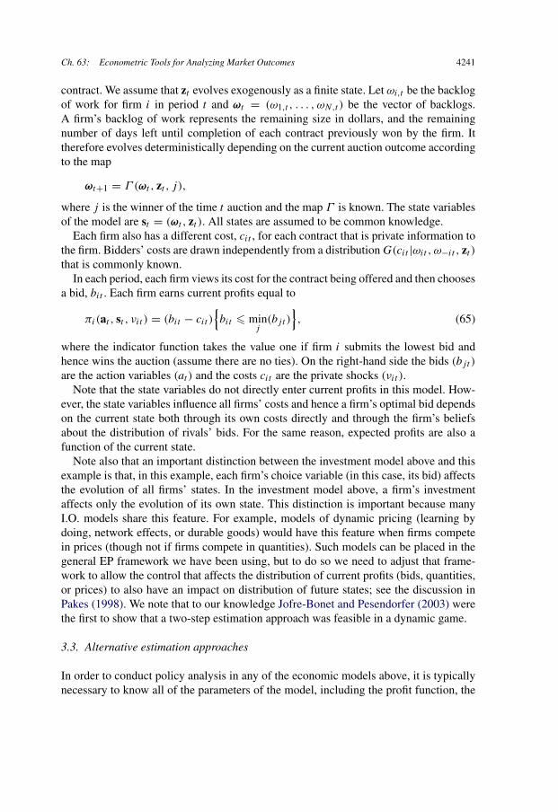
Ch. 63: Econometric Tools for Analyzing Market Outcomes 4241
contract. We assume that zt evolves exogenously as a finite state. Let ωi,t be the backlogof work for firm i in period t and ωt = (ω1,t , . . . , ωN,t ) be the vector of backlogs.A firm’s backlog of work represents the remaining size in dollars, and the remainingnumber of days left until completion of each contract previously won by the firm. Ittherefore evolves deterministically depending on the current auction outcome accordingto the map
ωt+1 = Γ (ωt , zt , j ),
where j is the winner of the time t auction and the map Γ is known. The state variablesof the model are st = (ωt , zt ). All states are assumed to be common knowledge.
Each firm also has a different cost, cit , for each contract that is private information tothe firm. Bidders’ costs are drawn independently from a distribution G(cit |ωit , ω−it , zt )
that is commonly known.In each period, each firm views its cost for the contract being offered and then chooses
a bid, bit . Each firm earns current profits equal to
(65)πi(at , st , νit ) = (bit − cit ){bit � min
j(bjt )
},
where the indicator function takes the value one if firm i submits the lowest bid andhence wins the auction (assume there are no ties). On the right-hand side the bids (bjt )
are the action variables (at ) and the costs cit are the private shocks (νit ).Note that the state variables do not directly enter current profits in this model. How-
ever, the state variables influence all firms’ costs and hence a firm’s optimal bid dependson the current state both through its own costs directly and through the firm’s beliefsabout the distribution of rivals’ bids. For the same reason, expected profits are also afunction of the current state.
Note also that an important distinction between the investment model above and thisexample is that, in this example, each firm’s choice variable (in this case, its bid) affectsthe evolution of all firms’ states. In the investment model above, a firm’s investmentaffects only the evolution of its own state. This distinction is important because manyI.O. models share this feature. For example, models of dynamic pricing (learning bydoing, network effects, or durable goods) would have this feature when firms competein prices (though not if firms compete in quantities). Such models can be placed in thegeneral EP framework we have been using, but to do so we need to adjust that frame-work to allow the control that affects the distribution of current profits (bids, quantities,or prices) to also have an impact on distribution of future states; see the discussion inPakes (1998). We note that to our knowledge Jofre-Bonet and Pesendorfer (2003) werethe first to show that a two-step estimation approach was feasible in a dynamic game.
3.3. Alternative estimation approaches
In order to conduct policy analysis in any of the economic models above, it is typicallynecessary to know all of the parameters of the model, including the profit function, the

4242 D. Ackerberg et al.
transition probabilities, and the distribution of the exogenous shocks. Often many of theparameters can be estimated “off line”, that is, without needing to compute equilibria ofthe dynamic game. At one extreme here is Benkard’s (2004) analysis of the commercialaircraft industry. He was able to obtain a large amount of cost data on sunk as well asmarginal costs which, together with generally available information on demand, enabledhim to estimate all the parameters he needed off line. Given these parameters he couldfocus on computing the dynamic implications of alternative policies.
However, such an approach is rarely possible. More typically, at least cost data areunavailable, either because they are proprietary and hence difficult for researchers toaccess, or because they are hard to measure. In static settings we often solve the prob-lem of a lack of cost data by inferring marginal costs from their implications in anequilibrium pricing equation. A similar approach can be taken in this dynamic setting.However, characterizing the relationship between the data generating process and equi-librium play in the models above is complicated by the fact that the model involvesrepeated interactions.
Observed behavior in the model represents the solution to a maximization problemthat involves both the profit function, which typically has a known parametric form,and the value function, which results from equilibrium play and therefore has unknownform. For example, the value of entering a market depends both on current profits, andexpected future profits, which in turn depend on future entry and exit behavior. In or-der to describe the data generating process, then, we need the ability to compute theequilibrium continuation values.
Thus, conceptually, estimation of dynamic models can be separated into two mainparts. The first part involves obtaining the continuation values for a given parametervalue, θ . The second part is to use the continuation values obtained in the first part tomaximize an objective function in the parameters, θ . Note that the continuation valuesmust be obtained for many different values of θ in order to perform this maximization,and thus the first part is the source of most of the computational burden of the estimation.The key differences in estimation approaches lie in the details of how each of these twoparts is performed.
3.3.1. The nested fixed point approach
The nested fixed point approach is a logical extension of the method of Rust (1987) togames. The general idea is as follows:
1. Given a parameter vector, θ , compute an equilibrium to the game, V (s; θ), numer-ically, using the computer.
2. Use the computed values, V (s; θ), to evaluate an objective function based on thesample data.
3. Nest steps one and two in a search routine that finds the value of θ that maximizesthe objective function.
A framework capable of computing equilibria to models like those above has existedfor some time [Pakes and McGuire (1994)], and recent papers by Pakes and McGuire

Ch. 63: Econometric Tools for Analyzing Market Outcomes 4243
(2001), Doraszelski and Judd (2004), and Weintraub, Benkard and Van Roy (2007) en-able significant improvements in computational times, at least in some problems [fora discussion of these, and other alternatives, see Doraszelski and Pakes (2007)]. All ofthese algorithms rely on similarities between the dynamic framework above and dy-namic programming problems. The general idea of these algorithms is to start with aninitial guess at the value function, V 0(s; θ), and substitute that into the right-hand sideof the Bellman equation (Equation (63)). Then, at each state point and for each firm,solve the maximization equation on the right-hand side of (63) yielding a new estimateof the value function, V 1(s; θ). This procedure is iterated until convergence is achieved,so that the new and old value functions are the same. Unlike single agent problems,in the context of a game, convergence of the algorithm is not guaranteed (the mappingis not a contraction) and, indeed, initial iterations will often seem to move away fromequilibrium. However, in practice the algorithms typically converge and, once they do,the value functions obtained must represent an equilibrium.
An important feature of the nested fixed point algorithm is that the first step is per-formed without using any data. As a result, the value functions are obtained precisely;that is, they contain no sampling error. This lack of sampling error makes the secondpart of the algorithm, in which the parameters are estimated, straightforward.
On the other hand the algorithm is computationally burdensome. For models richenough to use in empirical work, it is often difficult to compute an equilibrium evenonce, and in the nested fixed point algorithm it is necessary to compute an equilibriumonce for each iteration of the maximization routine; implying that up to hundreds, ifnot thousands, of fixed points must be calculated. Moreover, setting up an efficient al-gorithm often requires a large amount of complex computer programming, creating arelatively large burden on researcher time. As a result there are very few examples inthe literature where the nested fixed point algorithm has been applied to estimate para-meters.
One exception is Gowrisankaran and Town (1997), who use a nested fixed point ap-proach to apply a model similar to the investment model above to data for the hospitalindustry. In each iteration of the estimation they compute an equilibrium using the al-gorithm of Pakes and McGuire (1994). They then estimate the model using a GMMobjective function that matches cross-sectional moments such as average revenue perhospital, average expenditures per hospital, average investment per hospital, and aver-age number of hospitals of each type (nonprofit and for-profit) per market. The nestedfixed point approach was feasible in their application because their model was parsimo-nious and there were never more than three hospitals in any market in the data.
Another difficulty with the nested fixed point algorithm arises from the fact that dy-namic oligopoly models can admit more than one equilibria. While the assumptionsgiven above in principle allow the researcher to use the data to pick out the correct equi-librium, actually achieving this selection using the nested fixed point algorithm is likelyto be difficult. Moreover, equilibrium selection has to take place for every candidatevalue of the parameters to be estimated. Alternative sets of assumptions could be usedto select different equilibria, but unless we were willing to assume “a priori” that equi-
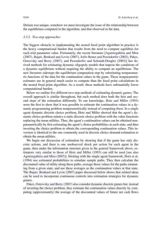
4244 D. Ackerberg et al.
librium was unique, somehow we must investigate the issue of the relationship betweenthe equilibrium computed in the algorithm, and that observed in the data.
3.3.2. Two-step approaches
The biggest obstacle to implementing the nested fixed point algorithm in practice isthe heavy computational burden that results from the need to compute equilibria foreach trial parameter value. Fortunately, the recent literature [Aguirregabiria and Mira(2007), Bajari, Benkard and Levin (2007), Jofre-Bonet and Pesendorfer (2003), Pakes,Ostrovsky and Berry (2007), and Pesendorfer and Schmidt-Dengler (2003)] has de-rived methods for estimating dynamic oligopoly models that impose the conditions ofa dynamic equilibrium without requiring the ability to compute an equilibrium. Thenew literature sidesteps the equilibrium computation step by substituting nonparamet-ric functions of the data for the continuation values in the game. These nonparametricestimates are in general much easier to compute than the fixed point calculations inthe nested fixed point algorithm. As a result, these methods have substantially lowercomputational burden.
Below we outline five different two-step methods of estimating dynamic games. Theoverall approach is similar throughout, but each method does both the first and sec-ond steps of the estimation differently. To our knowledge, Hotz and Miller (1993)were the first to show that it was possible to estimate the continuation values in a dy-namic programming problem nonparametrically instead of computing them. In a singleagent dynamic discrete choice problem, Hotz and Miller showed that the agent’s dy-namic choice problem mimics a static discrete choice problem with the value functionsreplacing the mean utilities. Thus, the agent’s continuation values can be obtained non-parametrically by first estimating the agent’s choice probabilities at each state, and theninverting the choice problem to obtain the corresponding continuation values. This in-version is identical to the one commonly used in discrete choice demand estimation toobtain the mean utilities.
We begin our discussion of estimation by showing that if the game has only dis-crete actions, and there is one unobserved shock per action for each agent in thegame, then under the information structure given in the general framework above, es-timators very similar to those of Hotz and Miller (1993) can still be used [see alsoAguirregabiria and Mira (2007)]. Sticking with the single agent framework, Hotz et al.(1994) use estimated probabilities to simulate sample paths. They then calculate thediscounted value of utility along these paths, average those values for the paths emanat-ing from a given state, and use these averages as the continuation values at that state.The Bajari, Benkard and Levin (2007) paper discussed below shows that related ideascan be used to incorporate continuous controls into estimation strategies for dynamicgames.
Pakes, Ostrovsky and Berry (2007) also consider dynamic discrete games but, insteadof inverting the choice problem, they estimate the continuation values directly by com-puting (approximately) the average of the discounted values of future net cash flows

Ch. 63: Econometric Tools for Analyzing Market Outcomes 4245
that agents starting at a particular state actually earned in the data (at least up to theparameter vector of interest). Econometrically, they use a nonparametric estimate of theMarkov transition probabilities that determine the evolution of the state of the system toform an analytic estimate of the probability weighted average of the discounted returnsearned from different states. Given equilibrium play, these averages will converge to thetrue expected discounted value of future net cash flow, that is of the continuation valueswe are after.
Bajari, Benkard and Levin (2007) instead begin by projecting the observed actions onthe state variables to compute nonparametric estimates of the policy functions of eachagent at each state. Then they use the estimated policies to simulate out the discountedvalues of future net cash flows. This procedure is computationally light even in modelswith large state spaces and is easily applied to models with continuous controls, such asinvestment, quantity, or price (including models with both discrete and continuous con-trols like the investment game above). Given equilibrium play, the continuation valuesobtained in this fashion will be consistent estimates of the continuation values actuallyperceived by the agents.
Berry and Pakes (2002) provide an alternative approach for estimating models withcontinuous controls that is likely to be useful when the dynamic environment is com-plex, but sales and investment data are available. They assume that current period netreturns are observable up to a parameter vector to be estimated, but do not require thatthe state variables of the model be observed, or even specified (so it would not be possi-ble to estimate policy functions conditional on those state variables as in Bajari, Benkardand Levin). They derive an estimating equation from the first order condition for thecontinuous control (investment in our example) by substituting observed profit streamsfor the expected profit streams, and noting that the difference must be orthogonal toinformation known at the time investment decisions are made.
Jofre-Bonet and Pesendorfer (2003) provide an estimator for the dynamic auctionmodel. They show that it is possible to derive an expression for the equilibrium contin-uation values in the auction game that involves only the bid distributions. Since bids areobserved, the bid distributions can be recovered nonparametrically from the data andthen substituted into these expressions. Provided that agents are bidding close to opti-mally, the continuation values obtained from this procedure will be consistent estimatesof the continuation values perceived by the agents.
In many of the cases we consider several of the methods could be used in estimation.In these cases it is not currently known how the methods compare to one another onsuch dimensions as computational burden and econometric efficiency. Hybrid methodsare also possible in which features of two or more of the approaches could be combined.We expect these issues to be sorted out in the future.
Finally, there are also some costs associated with the two-step approaches. First, be-cause the continuation values are estimated rather than computed, they contain samplingerror. This sampling error may be significant because these models often have statespaces that are large relative to the available data. As we will see below, this influ-ences the properties of the second step estimators in important ways. To summarize, the

4246 D. Ackerberg et al.
choice of second stage estimation method will be influenced as much or more by a needto minimize small sample bias caused by error in the continuation value estimates as itis by the desire to obtain asymptotic efficiency.
Second, for the two step approaches to produce estimators with desirable propertiesthe data must visit a subset of the points repeatedly. Formally the requirement for thelimit properties of the estimators is that all states in some recurrent class R ⊆ S bevisited infinitely often. Moreover, equilibrium strategies must be the same every timeeach point in R is visited. Whether or not this assumption is reasonable for the problemat hand depends on the nature of the available data and the institutional setting whichgenerated it. If the data consists of a time series on one market then we would requirestationarity of the process over time. There are different ways to fulfill this requirementin panels (i.e. when we follow a cross section of markets over time); one possibility isthat the initial state in each market is a random draw from a long run ergodic distribution.Note that the nested fixed point approach has a weaker data requirement.
These costs must be weighed against the benefit that the two-step estimators eliminatemost of the computational burden of the nested fixed point approach. Indeed, the entiretwo-step algorithm might well have less computational burden than one iteration of thenested fixed point algorithm.
3.4. A starting point: Hotz and Miller
Because of the similarity of this section to the previous literature on single agent prob-lems, we will keep this section short, concentrating mainly on extending Hotz and Millerto games. For more detail on the approach in single agent problems see Hotz and Miller(1993), Hotz et al. (1994), Magnac and Thesmar (2002), and Rust (1994). See alsoAguirregabiria and Mira (2007) and Pesendorfer and Schmidt-Dengler (2003) for a dis-cussion in the context of entry games.
The idea behind Hotz and Miller’s estimation method for single agent problems is toset up a dynamic discrete choice problem such that it resembles a standard static discretechoice problem, with value functions taking the place of standard utility functions. Thisallows a two step approach in which a discrete choice model is used as a first step forrecovering the value functions, and the parameters of the profit function are recoveredin a second step once the value functions are known.
We make two simplifying assumptions that will assist in the exposition. First, wesuppose that agents’ current profits do not depend on rivals’ actions (though they dodepend on rival’s states whose evolution depends on those actions). Second, we assumethat the unobserved shocks are additive to profits. In that case, current profits are givenby
πi(at , st , νit ) = π (ait , st ) + νit (ait ),
where νit is agent i’s vector of profitability shocks and νit (ait ) is the shock associatedwith agent i’s action ait .

Ch. 63: Econometric Tools for Analyzing Market Outcomes 4247
The first assumption simplifies the agents’ choice problem because, if agents’ currentprofits depend on rivals’ actions then, since rivals’ actions depend on their own currentshocks, in its own maximization problem each agent would have to integrate currentprofits over all rivals’ current actions. This would not change the overall approach butwould complicate the computations below [we would need to integrate over distribu-tions of competitors outcomes to compute the expected profits; see Aguirregabiria andMira (2007) for a model in which profits do depend on rivals’ actions]. The secondsimplification, additive separability in the private shocks, is also not strictly required.If the error terms entered profits nonlinearly then we could rewrite the problem interms of expected profits and an additively separable projection error and work withthat framework instead. However, such an approach does have the unattractive prop-erty that it changes the interpretation of the profit function. Thus, it is typically thecase that in practice people assume that the profit function has additive structural errorterms.
With these assumptions the Bellman equation can be simplified to (suppressing thesubscripts)
(66)V (s, ν) = maxa
{π(a, s) + ν(a) + β
∫V (s′, ν′) dG(ν ′|s′) dP(s′|s, a)
}.
Equation (66) represents a discrete choice problem in which the mean utilities are givenby
(67)va(s) = π (a, s) + β
∫V (s′, ν′) dG(ν ′|s′) dP(s′|s, a).
Thus, since the private shocks are independent across time and across agents, the choiceprobabilities for a given agent can be generated in the usual manner of a static discretechoice problem
(68)Pr(a|s) = Pr(va(s) + ν(a) � va′(s) + ν(a′),∀a′).
Assuming that the data consists of a large sample of observations on states and ac-tions, the probability of each action at each state, Pr(a|s), can be recovered from thedata. In that case, the left-hand side of (68) is known, at least asymptotically. Let P(s)be the vector of choice probabilities for all feasible actions. Hotz and Miller show thatfor any distribution of the private shocks there is always a transformation of the choiceprobabilities such that
(69)va(s) − v1(s) = Qa
(s, P (s)
).
That is, the differences in the choice specific value functions can be written as a func-tion of the current state and the vector of choice probabilities. The transformation onthe right-hand side is the same as the inversion used in the discrete choice demand es-timation literature. Berry (1994) proves that the solution is unique. Berry, Levinsohnand Pakes (1995) provide a transformation from the data to the mean utilities which is

4248 D. Ackerberg et al.
a contraction, and hence enables the researcher to actually compute the mean utilities(for more discussion see the first part of this chapter).
In general, this transformation can be used to recover the normalized choice specificvalue functions, va−v1, at each state, using the estimated choice probabilities. If the dis-tribution of the private shocks is known, the mapping does not depend on any unknownparameters. For example, in the case of the logit
(70)Qa
(s, P (s)
) = ln(Pr(a|s))− ln
(Pr(a1|s)
).
However, in general the mapping may be a function of unknown parameters of thedistribution of the private shocks.
Note that, as in static discrete choice models, only the value differences can be recov-ered nonparametrically. Thus, some further information is required to obtain the valuesthemselves. This difficulty is not just a feature of this particular estimation approach,but comes from the underlying structure of the discrete choice framework, in whichonly utility differences are identified from the observed choices. One consequence ofthis is that, even if the discount factor and the distribution of private shocks are com-pletely known, the profit function cannot be recovered nonparametrically [see Magnacand Thesmar (2002) for a detailed proof and analysis for single agent dynamic discretechoice problems, and Pesendorfer and Schmidt-Dengler (2003) for results extended todynamic discrete games]. This feature is inherent to the dynamic discrete choice setupand carries through to the context of a dynamic discrete game. As noted earlier our feel-ing is that the appropriate resolution of identification issues, such as this one, is contextspecific and will not be discussed here.
To obtain the continuation values from the choice specific values we can use the factthat
(71)V (s, ν) = maxa
{va(s) + ν(a)
}.
Because the continuation values are obtained by inverting from the observed choiceprobabilities, the structure of the profit function has not yet been imposed on them, andthey are not yet functions of the profit function parameters. In order to estimate theprofit function parameters, Hotz and Miller iterate the Bellman equation once, insertingthe estimated continuation values on the right-hand side,
V (s; θ) =∫
maxa
{π (a, s; θ) + ν(a)
(72)+ β
∫V (s′, ν′) dG(ν ′|s′) dP(s′|s, a)
}dG(ν|s).
Note that for some distributions such as those of type GEV the integral on the right-handside has an analytic form. In other cases it can be simulated.
These new estimates of the continuation values contain the profit function parameters(θ ) and can be used in an estimation algorithm to estimate θ . The way this is typically
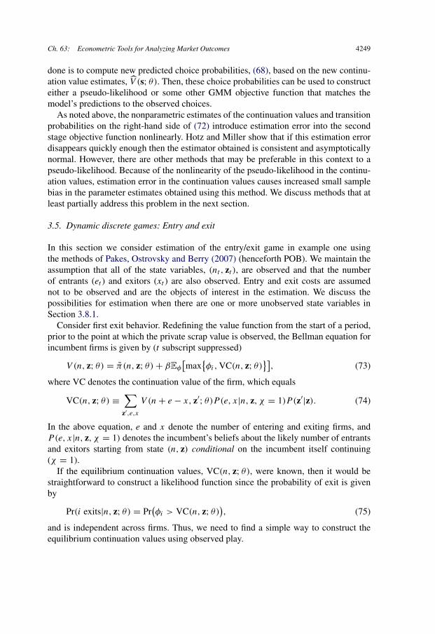
Ch. 63: Econometric Tools for Analyzing Market Outcomes 4249
done is to compute new predicted choice probabilities, (68), based on the new continu-ation value estimates, V (s; θ). Then, these choice probabilities can be used to constructeither a pseudo-likelihood or some other GMM objective function that matches themodel’s predictions to the observed choices.
As noted above, the nonparametric estimates of the continuation values and transitionprobabilities on the right-hand side of (72) introduce estimation error into the secondstage objective function nonlinearly. Hotz and Miller show that if this estimation errordisappears quickly enough then the estimator obtained is consistent and asymptoticallynormal. However, there are other methods that may be preferable in this context to apseudo-likelihood. Because of the nonlinearity of the pseudo-likelihood in the continu-ation values, estimation error in the continuation values causes increased small samplebias in the parameter estimates obtained using this method. We discuss methods that atleast partially address this problem in the next section.
3.5. Dynamic discrete games: Entry and exit
In this section we consider estimation of the entry/exit game in example one usingthe methods of Pakes, Ostrovsky and Berry (2007) (henceforth POB). We maintain theassumption that all of the state variables, (nt , zt ), are observed and that the numberof entrants (et ) and exitors (xt ) are also observed. Entry and exit costs are assumednot to be observed and are the objects of interest in the estimation. We discuss thepossibilities for estimation when there are one or more unobserved state variables inSection 3.8.1.
Consider first exit behavior. Redefining the value function from the start of a period,prior to the point at which the private scrap value is observed, the Bellman equation forincumbent firms is given by (t subscript suppressed)
(73)V (n, z; θ) = π(n, z; θ) + βEφ
[max
{φi, VC(n, z; θ)
}],
where VC denotes the continuation value of the firm, which equals
(74)VC(n, z; θ) ≡∑
z′,e,xV (n + e − x, z′; θ)P (e, x|n, z, χ = 1)P (z′|z).
In the above equation, e and x denote the number of entering and exiting firms, andP(e, x|n, z, χ = 1) denotes the incumbent’s beliefs about the likely number of entrantsand exitors starting from state (n, z) conditional on the incumbent itself continuing(χ = 1).
If the equilibrium continuation values, VC(n, z; θ), were known, then it would bestraightforward to construct a likelihood function since the probability of exit is givenby
(75)Pr(i exits|n, z; θ) = Pr(φi > VC(n, z; θ)
),
and is independent across firms. Thus, we need to find a simple way to construct theequilibrium continuation values using observed play.

4250 D. Ackerberg et al.
The continuation values represent the expected discounted value of future profitsconditional on the incumbent continuing. They are a function of the profit function,π(n, z; θ), which determines future profits at each state (n, z), and the processes deter-mining the evolution of the state variables, n and z. The profit function is known up tothe parameters, θ . Therefore, in order to construct the continuation values as a functionof the parameters, we need only estimate the evolution of the number of firms, whichis determined by entry and exit, and the evolution of the profit shifters, P(z′|z). Theeasiest way to do this is to use their empirical counterparts. Starting from a certain state,to estimate the evolution of the number of firms we can use the actual evolution of thenumber of firms each time that state was observed in the data. Similarly, we can usethe observed evolution of the profit shifters to estimate the process P(z′|z). That waythe estimated continuation values reflect, approximately, the actual profits of firms thatwere observed in the data. The next subsection outlines this process in detail.
3.5.1. Step 1: Estimating continuation values
To facilitate estimation of the continuation values, it helps to rewrite the Bellman equa-tion in terms of the continuation values, VC,
VC(n, z; θ) =∑n′,z′
[π(n′, z′; θ)
(76)+ βEφ
[max
{φi, VC(n′, z′; θ)
}]]P(n′|n, z, χ = 1)P (z′|z),
where to shorten the notation we let n′ ≡ n + e − x.Next, rewrite (76) in vector form. Let VC(θ) be the #S × 1 vector representing
VC(n, z; θ) for every (n, z) pair, and define π(θ) similarly. Also let Mi be the #S × #Smatrix whose (i, j) element is given by P(nj |ni, zi, χ = 1)P (zj |zi). This is the matrixwhose rows give us the equilibrium transition probabilities from a particular (n, z) toeach other possible (n, z). Note that if we were not conditioning on χ = 1 an unbiasedestimate of the rows of this matrix could be obtained by simply counting up the fractionof transits from (n, z) that were to each other state. Since the continuation value theagent cares about is the continuation value should the agent continue, these estimateshave to be modified for conditioning on χ = 1, see the discussion below.
With this notation, (76) becomes
(77)VC(θ) = Miπ(θ) + βMiEφ
[max
{φi, VC(θ)
}].
In this last equation, π(θ) is a known vector (up to θ ). In a structural model the dis-tribution of φ would also typically be known up to a parameter vector. Therefore, theonly unknowns in the equation are Mi and VC(θ). If Mi were known, VC(θ) could becalculated as the solution to the set of equations (77). We discuss the estimation of Mi
below and turn first to the solution for VC(θ).One of the insights of POB is that the expectations term on the right-hand side of (77)
can sometimes be simplified, making computation of VC(θ) simple. Expanding the

Ch. 63: Econometric Tools for Analyzing Market Outcomes 4251
expectations term at a single state (n, z) gives
Eφ
[max
{φi, VC(n, z; θ)
}]= Pr
(φi < VC(n, z; θ)
) ∗ VC(n, z; θ)
+ Pr(φi > VC(n, z; θ)
) ∗ Eφ
[φi
∣∣φi > VC(n, z; θ)]
= (1 − px(n, z)) ∗ VC(n, z; θ) + px(n, z) ∗ Eφ
[φi
∣∣φi > VC(n, z; θ)],
where px(n, z) is the probability of exit at state (n, z). Provided that the distribution ofscrap values is log-concave, the above equation is a contraction mapping [see Heckmanand Honoré (1990)]. In that case, given estimates of Mi and px , the equation can besolved for VC(·) in a straightforward manner. Moreover, when the distribution of scrapvalues is exponential, a distribution often thought to be reasonable on a priori grounds,
Eφ
[φi
∣∣φi > VC(n, z; θ)] = σ + VC(n, z; θ),
where σ is the parameter of the exponential, and
Eφ
[max
{φi, VC(n, z; θ)
}]= (1 − px(n, z)
) ∗ VC(n, z; θ) + px(n, z) ∗ [VC(n, z; θ) + σ]
= VC(n, z; θ) + σpx(n, z).
Substituting this expression into (77) and iterating gives
VC(θ) = Mi[π(θ) + βσpx
]+ (Mi)2[
π(θ) + βσpx
]+ (Mi)3
VC(θ) + · · ·
=∞∑
τ=1
(Mi)τ [
π(θ) + βσpx
](78)= (I − βMi
)−1Mi[π(θ) + βσpx
].
The only thing that remains is to estimate Mi and px using the data. Both can be esti-mated in a variety of different ways, but the simplest approach, and the one supportedby POB’s Monte Carlo results, is to use their empirical counterparts. Let
T (n, z) = {t : (nt , zt ) = (n, z)}
be the set of periods in the data with the same state (n, z). Then, the empirical counter-part to px is
px(n, z) = 1
#T (n, z)
∑t∈T (n,z)
xt
n.
Due to the Markov property, px(n, z) is a sum of independent draws on the exit proba-bility, and therefore it converges to px(n, z) provided #T (n, z) → ∞.
Similarly, the matrix Mi can be estimated element-by-element using
Mii,j =
∑t∈T (ni ,zi )
(ni − xt )1{(nt+1, zt+1) = (nj , zj )}∑t∈T (ni ,zi )
(ni − xt ).

4252 D. Ackerberg et al.
This expression weights the actual observed transitions from (ni, zi) in different periodsby the number of incumbents who actually continue in those periods. This weightingcorrects the estimated transition probabilities for the fact that incumbents compute con-tinuation values under the assumption that they will continue in the market.
Note that because this procedure uses empirical transition probabilities it never re-quires continuation values or transition probabilities from points not observed in thedata. As a result there is no need to impute transition probabilities or continuation val-ues for states not visited.55 Since typical data sets will only contain a small fraction ofthe points in S, this reduces computational burden significantly.
Substituting the estimated transition and exit probabilities into (78) provides an ex-pression for the estimated continuation values
(79)VC(θ, σ ) = (I − βMi)−1
Mi[π(θ) + βσ px
].
Note first that the estimates of continuation values using the expression in (79) are,approximately, the averages of the discounted values of the incumbents who did con-tinue.56 This makes the relationship between the data and the model transparent. Pro-vided only that the specification of the profit function is correct, the actual average ofrealized continuation values should be close to the expected continuation values usedby the agents in making their decisions.
Second, note how easy it is to compute the estimated continuation values. If the dis-count factor is known, then,
(80)VC(θ, σ ) = Aπ(θ) + aσ,
where A = (I − βMi)−1Mi and a = β(I − βMi)−1px . Both A and a are independentof the parameter vector and can therefore be computed once and then held fixed in thesecond step of the estimation.
Finally, note that the parameters of the entry distribution do not enter into the calcu-lation of the continuation values. The reason for this is that sunk costs of entry are paidonly once at the time of entry. After that, the sunk costs distribution only affects profitsindirectly through rival firms’ entry decisions. Thus, all that matters for computing con-tinuation values is the probability of entry, not the associated level of sunk costs. As aresult the computational burden of the model does not depend in any major way on theform of the entry cost distribution, a fact which is particularly useful when we considermodels with multiple entry locations below.
Entry behavior can be described similarly. A potential entrant enters the market ifthe expected discounted value of entering is greater than the entry cost, i.e. if χe is the
55 Strictly speaking this is only true if the last period’s state in the data was visited before. If it were not wewould have to impute transition probabilities for it.56 This is only approximately true because the transitions for all firms that reached a state (n, z) are used tocompute transitions for each firm, so information is pooled across firms in computing the continuation values.

Ch. 63: Econometric Tools for Analyzing Market Outcomes 4253
indicator function which is one if the potential entrant enters and zero elsewhere
β VE(n, z; θ) � κ,
where
VE(n, z; θ) ≡∑
z′,e,xV (n + e − x, z′; θ)P
(e, x∣∣n, z, χe = 1
)P(z′|z),
similarly to VC before. The main difference here is that the entrant is not active in thecurrent period and therefore forms beliefs slightly differently from the incumbent.
The incumbent forms beliefs conditional on it remaining active. The entrant formsbeliefs based on it becoming active. In vector form, the expression for the entrants’continuation values is
VE(θ, σ ) = Me(π + β VC(θ) + βpxσ
),
where the elements of Me represent a potential entrant’s beliefs about the distributionover tomorrow’s states conditional on that entrant becoming active. An estimator forMe that is analogous to the one above is given by
Mei,j =
∑t∈T (ni ,zi )
et1{(nt+1, zt+1) = (nj , zj )}∑t∈T (ni ,zi )
et
.
Accordingly, a consistent estimator of VE(θ, σ ) is given by
(81)VE(θ, σ ) = Bπ(θ) + bσ,
where B = Me(I + βA), and b = βMe(a + px).
3.5.2. Step 2: Estimating the structural parameters
If the continuation values (VE and VC) were known, any of a number of method ofmoments algorithms would provide consistent estimators of (θ, σ ) and maximum like-lihood would provide the efficient estimator. Since VE and VC are consistent estimatorsof the unknown continuation values, an obvious way to obtain a consistent estima-tor is to substitute them for VC and VE in any of these algorithms and proceed fromthere. For example, the implied “pseudo” maximum likelihood estimator would maxi-mize
l(xt , et |θ, σ ) = (nt − xt ) log Fφ[VC(nt , zt ; θ, σ )
]+ xt log
[1 − Fφ
(VC(nt , zt ; θ, σ )
)]+ et log Fκ
[VE(nt , zt ; θ, σ )
]+ (E − et ) log
[1 − Fκ
(VE(nt , zt ; θ, σ )
)],
where Fφ is the distribution of scrap values and Fκ is the distribution of entry costs.

4254 D. Ackerberg et al.
POB stress the importance of remembering that VE and VC contain sampling error.Though this sampling error does converge to zero with sample size, the fact that wehave to estimate separate continuation values for each sample point means that, forstandard sample sizes, the sampling error should not be ignored. This has implicationsboth for the choice of estimators, and for how we compute standard errors for any givenchoice.
In this context there are two problems with the pseudo maximum likelihood estimator.First since it does not “recognize” that there is sampling error in the probabilities it uses,events can occur that the likelihood assigns zero probability to, no matter the value of(θ, σ ) (even though the true probabilities of these events are nonzero; POB shows thatthis tends to occur in their two location model). If this happens even once in the data,the pseudo maximum likelihood estimator is not defined. Second, even if the pseudo-likelihood is well defined, its first order condition involves a function that is both highlynonlinear in, and highly sensitive to, the sampling error. The nonlinearity implies thatthe impact of the sampling error on the first order conditions will not average out oversample points. The sensitivity is seen by noting that the first order effect of the samplingerror on the log likelihood will be determined by one over the probabilities of entry andexit, and these probabilities are typically quite small.
POB consider two alternatives to the likelihood approach. The first is a pseudo min-imum χ2 estimation algorithm that minimizes the sum of squares in the differencebetween the observed and predicted state specific entry and exit rates (i.e. the entryand exit rates for each observed (n, z) pair), where the predicted state specific entry andexit rates are given by
E[xt |nt , zt ] = nt ∗ Pr(φi > VC(nt , zt ; θ, σ )
), and
E[et |nt , zt ] = E ∗ Pr(κ < VE(nt , zt ; θ, σ )
).
Their second estimator matches the overall entry and exit rates (across all observedstate pairs) to those predicted by the model, or more generally takes a sum of squares inthe differences between the predicted and actual entry and exit rates at different statesmultiplied by a known function of the state variables at those states.
They show that in finite samples the pseudo minimum χ2 estimator has an extra biasterm that reflects the sampling covariance between the estimated probability and itsderivative with respect to the parameter vector, and their Monte Carlo evidence indicatesthat the extra bias term can have large effects. Thus they prefer the simplest method ofmoments algorithm and show that with moderately sized samples this estimator is botheasy to calculate and performs quite well.
The second general point is that the variance of the second stage estimates, (θ , σ ),depends on the variance of the first stage estimates.57 It is possible to use standardsemiparametric formulae to obtain the asymptotic variance of the parameter estimates
57 This follows from the fact that the derivative of the objective function with respect to the estimates of VCand VE are not conditional mean zero.

Ch. 63: Econometric Tools for Analyzing Market Outcomes 4255
analytically. However these formula are somewhat complex and can be difficult to eval-uate. Moreover, there is little reason to do the calculation. Since we have a completemodel and the computational burden of obtaining estimates is minimal it is relativelyeasy to obtain estimates of standard errors from a parametric bootstrap.
For an empirical example which uses these techniques see Dunne et al. (2006). Theyestimate the parameters of a dynamic entry game from data on entry and exit of dentistsand chiropractors in small towns. They first estimate the variable profit function (whichdepends on the number of active competitors) from observed data on revenues and costs.They then employ POB’s method to provide estimates of the sunk costs of entry andof exit values. Their parameters could be used, for example, to predict the effect of agovernment subsidy intended to increase the number of medical service professionalsin small towns.
3.5.3. Multiple entry locations
We now show how to generalize the model to allow for observed heterogeneity amongincumbents. We do this by allowing entrants to choose from multiple entry locations.For ease of exposition, we will consider only two locations. However, expanding this toa larger number is straightforward.
Entrants have entry costs (κ1, κ2) in the first and second locations respectively, whereentry costs are drawn from a distribution, Fκ(κ1, κ2|θ), that is independent over timeand across agents. Note that we place no restrictions on Fκ so that entry costs of thesame potential entrant at the different locations may be freely correlated. Once in aparticular location, the entrant cannot switch locations, but can exit to receive an exitfee. Exit fees are an i.i.d. draw from the distribution F
φ1 (·|θ) if the incumbent is in
location one, and an i.i.d. draw from Fφ2 (·|θ) if the incumbent is in location two.
The Bellman equation for an incumbent in the two location model is
V1(n1, n2, z; θ) = π1(n1, n2, z; θ) + βEφ
[max
{φi, VC1(n1, n2, z; θ)
}],
where the subscript “1” indicates the value function for a firm in location one and thecontinuation values are
VC1(n1, n2, z; θ) ≡∑
z′,e1,e2,x1,x2
V1(n1 + e1 − x1, n2 + e2 − x2, z′; θ)
× P(e1, e2, x1, x2|n1, n2, z, χ = 1)P (z′|z).Behavior of incumbent firms is identical to before, with the probability of exit givenby (75) except using the new continuation values. However, because they have poten-tially different continuation values and different scrap values, firms in location one willin general behave differently than firms in location two.
Behavior of potential entrant firms is different from before because potential entrantfirms now have three options. They can enter location one, enter location two, or notenter at all. A potential entrant will enter into location 1 if and only if it is a better

4256 D. Ackerberg et al.
alternative than both not entering anywhere, and entering into location 2, i.e. if
β VE1(n1, n2, z; θ) � κ1 and
β VE1(n1, n2, z; θ) − κ1 � β VE2(n1, n2, z; θ) − κ2.
The entry process therefore generates a multinomial distribution with probabilities de-rived from the inequalities above.
Firms’ beliefs are now comprised of the probability of exit for an incumbent in lo-cation one, the probability of exit for an incumbent in location two, the three entryprobabilities (location one, location two, or not at all), and the distribution determiningthe evolution of the profit shifters. In computing the continuation values we now haveto consider all of these together.
Consistent estimates of a location-one incumbent’s perceived transition probabilitiesfrom state (ni1, ni2, zi) to (nj1, nj2, zj ) are obtained analogously to before using
Mi,1i,j =
∑t∈T (ni1,ni2,zi )
(ni1 − xt1)1{(nt+1,1, nt+1,2, zt+1) = (nj1, nj2, zj )}∑t∈T (ni1,ni2,zi )
(ni1 − xt1).
Similarly, estimates of a potential location-one entrant’s perceived transition probabili-ties can be obtained using
Me,1i,j = 1
#T (ni1, ni2, zi)
×∑
t∈T (ni1,ni2,zi )et11{(nt+1,1, nt+1,2, zt+1) = (nj1, nj2, zj )}∑
t∈T (ni1,ni2,zi )et1
.
As before these estimates are not exactly equal to the empirical frequency of state tran-sitions but are a weighted average based on the fact that, when computing continuationvalues, an incumbent assumes it will continue, and a potential entrant assumes that itwill enter.
As in the single location model, given the matrix inversion formula for continuationvalues, the computational burden of obtaining estimates for the parameters of the modelis minimal. Indeed in their Monte Carlo results POB show that in two location modelswith relatively large data sets (on the order of 7500 observations) one finds estimatesin under fifteen minutes on a five year old desktop computer. Most of that computationtime is devoted to computing the Markov transition matrix and its inverse. The timerequired to compute the inverse can grow polynomially in the number of distinct statesand, at least given market size, this typically increases with the number of locations.Whether it does or not depends on the structure of the matrix being inverted, and theway one computes the inverse. Models which only allow transitions to “near by” states,which are likely to dominate in I.O. applications, should not be as problematic in thisrespect.
Second, though the estimators remain consistent when the number of entry states isincreased, their small sample properties may change. In particular, the estimates of thecontinuation values will become noisier in small samples and this is likely to cause

Ch. 63: Econometric Tools for Analyzing Market Outcomes 4257
increased small sample bias and variance in the second stage estimates. POB show thatthe use of smoothing techniques, such as those discussed in the next section, can behelpful in this context.
3.6. Models with discrete and continuous controls: Investment games
In this section we consider Bajari, Benkard and Levin’s (2007) (henceforth BBL) es-timation approach in the context of the investment model in example two. The mainconceptual difference in BBL’s general approach that separates it from the above meth-ods is that, instead of estimating continuation values directly, BBL first estimate policyfunctions. Then, the estimated policy functions are used to simulate the continuationvalues. As noted earlier this is similar to the single agent approach of Hotz et al. (1994),but BBL show that there are assumptions and techniques that allow the researcher touse this approach in a wide class of models, including models with both discrete andcontinuous controls such as investment models, some models of dynamic pricing, anddynamic auction problems. The assumptions used do carry with them some restrictions,and we will try to be clear on those restrictions below.
The presence of both discrete and continuous controls in the investment model af-fects both the first and second stage of the estimation. In particular, the second stageis augmented in order to incorporate information from firms’ investment, as well as itsentry/exit, choices. Additionally, when the stress is on investment we generally considermodels with larger state spaces, and, as noted above, both computation of the estimatesof continuation values, and the precision of those estimates, can become problematic.BBL introduce simulation techniques that, depending on the structure of the model,can cause a significant reduction in the computational burden of obtaining estimates ofthe continuation values. They also use techniques that smooth estimated continuationvalues across states to lower the mean square error of those estimates.
In the investment model from example two there are three policies (entry, exit, andinvestment) that are set in dynamic equilibrium, and one policy (price) that is set instatic equilibrium. Since the pricing equilibrium is consistent with a large past literatureon demand estimation, we will not consider estimation of the demand and marginal costfunctions (θ1 and θ2) here as they would typically be estimated using existing methods.Instead, we will treat those parameters as if they were known and focus on estimationof the investment cost function (θ3) and the entry and exit costs parameters.
We assume that all of the state variables, s, are observed, as well as entry, exit, quan-tity, price, and investment levels. Entry and exit costs, the cost of investment function,and marginal costs are not observed. Note that it would be possible for some of thestate variables to be unobserved as long as they could be recovered beforehand duringestimation of the demand and cost systems. We discuss the issue of unobserved statesfurther in Section 3.8.1.
Let πi(s) represent the profits earned by firm i in the spot market equilibrium atstate s. Since the demand and marginal cost functions are assumed to be known, the

4258 D. Ackerberg et al.
function πi (·) is also known, as the spot market equilibrium can be computed fromthese primitives.
Firms maximize the expected discounted value of profits. From the beginning of aperiod (prior to realization of the private shock), and for incumbent firms, this is
(82)E
∞∑t=0
βt[{χit = 1}(πi(st ) − C(Iit , νit ; θ3)
)+ (χit − χi,t−1)−Φ∣∣s0],
where χit = 1 indicates that the incumbent continues in the market at period t andχit = 0 indicates that the incumbent exits, and it is understood that each exiting firmreceives the same exit value and never operates thereafter. Note that unlike in the en-try/exit example above, in this model we assume that the incumbent’s choice of itsdiscrete control (whether or not to exit) is not subject to a random cost shock.
For expositional (and computational) simplicity we will assume the followingquadratic cost of investment function
(83)C(I, ν; θ3) = {I � 0}(θ3,0 + θ3,1I + θ3,2I2 + θ3,3νI
).
The indicator function for I � 0 above allows for an adjustment cost that is incurredonly if investment is nonzero. Zero investment is a phenomenon that is often observedand can easily result from either flatness of the value function reflecting low returnsto investment [see Ericson and Pakes (1995)], or nonconvex investment costs [e.g.Caballero and Engel (1999)].
Potential entrant firms’ expected discounted values are similar to (82), except that inthe initial period they must pay a random entry cost, κit , in order to enter. We assumethat entrants take one period to setup the firm and therefore do not earn profits in thespot market and do not invest until the subsequent period. For ease of exposition, wealso assume that entrants always enter at the same initial state.58
3.6.1. Step 1: Estimating continuation values
The goal of the first step of the estimation procedure is to compute the continuationvalues given by the expected discounted values in (82), under equilibrium strategies.These expected discounted values are functions of the profits earned at each state andthe probability distributions determining future states and actions conditional on thestarting state, s0.
BBL compute estimates of the continuation values by first estimating policies foreach state, then using the estimated policies to simulate sample paths of industry statesand actions, and then evaluating discounted profits on each sample path. In order to dothis we need both the ability to simulate sample paths of states and actions, and theability to evaluate profits along those paths given the states and actions in each period.
58 It is straightforward to allow entrants’ initial state to be randomly determined.

Ch. 63: Econometric Tools for Analyzing Market Outcomes 4259
Evaluating profits requires a (possibly flexible) description of the profit function andknowledge of the distribution of the private shocks, at least up to a parameter vector tobe estimated. We treat these two as “primitives” of the dynamic model.
The evolution of the states depends on firms’ entry, exit, and investment policies. BBLrecover these policy functions using the observed data. In our investment model, privateinformation is known to the firms before any actions are taken, so in MPE, strategies forinvestment, exit and entry are functions of both the states and this private information
I (st , νit ), χ(st , νit ), and χe(st , κit ),
where χ is the exit policy function for incumbent firms, χe is the entry policy functionand χe = 1 indicates that the entrant enters the market. Since potential entrants cannotinvest in the first period, entry strategies depend only on the random entry cost. Boththe investment and exit strategies depend only on the shock to the marginal cost ofinvestment.
Consider first exit and entry. The optimal exit policy has the form of a stopping rule
χi,t = 1 iff νit � ν(st ).
All we require is a nonparametric estimate of the probability that χ = 1 conditionalon st . Similarly, there a critical entry level of κ conditional on st that determines entry,and the entry policy is obtained as a nonparametric estimate of the probability of entryconditional on st . In both cases we also have the restriction that the policies are ex-changeable in rivals’ states. In models with large state spaces, such that there are somestates in the data with few or zero observations, it would typically be optimal to employsome smoothing in these estimates. In their Monte Carlo studies, BBL found that locallinear methods worked well for this.
As far as investment is concerned, one can show that, conditional on a firm continuingin the market, investment is a (weakly) monotone function of νit , I (st , νit ). Thus, if weknew the distribution of investment at each state, F(Iit |st ), we could map the quantilesof ν into investment levels at each state. More precisely, the investment policy functionis given by
F−1I |s(G(ν|s)).
The function G is a primitive of the model known up to a parameter vector, and thefunction F can be recovered nonparametrically.
There is an additional complication and that is that investment is not observed forfirms that exit the market, which happens if νit > ν(st ). However, since both the exitand investment rules are monotonic in the shock, this is handled easily. Conditional ona firm continuing in the market, we observe the distribution of investment conditionalon s that corresponds to νit � ν(st ). Therefore, if we first estimate the probability of exitat each state, and then recover the distribution of investment at each state conditionalon staying in the market, then we have a complete description of the optimal exit and

4260 D. Ackerberg et al.
investment policy functions.59 Note also that in the simulations below it is importantthat we maintain this link between exit and investment since one draw on the privateshock to investment, νit , determines both policies.
If there was a second unobservable, say a random exit fee φit , then the exit decisionwould depend on both (νit , φit ). The probability of exit could still be obtained as above,but the distribution of investment conditional on not exiting would depend on both νit
and φit . Then, without further restrictions it would not be possible to invert the observeddistribution of investment to obtain the policy decision as a function of ν conditionalon s and not exiting.60
There also remains the question of how best to estimate the investment function, andthis depends to some extent on its likely properties. Here it is important to keep in mindthat investment is a complicated function of the primitives. Indeed the only restrictionwe have on its form is that it is exchangeable in the states of the competitors (which isalready embodied in the definition of s). Standard nonparametric approaches assume acertain amount of smoothness that is not necessarily guaranteed by the primitives of themodel. The theoretical properties of the investment function in the EP model dependon the underlying properties of the family {P(sit+1|Iit , sit )}. If conditional on sit thepoints of support of this family do not depend on Iit ,61 then by appropriate choice ofprimitives one can ensure that the investment function is smooth; see EP, the MonteCarlo evidence in BBL, and the generalizations of this in Doraszelski and Satterthwaite(2007). In their Monte Carlo studies BBL also found that local linear regression workedwell for estimating the investment function.
Assume now that, for each state, we have consistent estimators of the entry probabil-ity, the exit probability, the investment distribution, and the distribution of future states.This is all one needs to compute consistent estimates of the continuation values in (82)as a function of the parameters. To do so analytically, however, would involve high di-mensional integration, so what BBL do is show how to extend the “forward simulation”idea in Hotz et al. (1994) to simplify the analysis of the more complex problems theydeal with.
Starting from a given state, s0, one draw is taken on the shock to the marginal costof investment for the firm of interest, νi . This draw determines the firm’s investmentand exit policies through the estimated policy functions above (i.e. the same draw de-termines the correct quantile for both investment and exit, as discussed above). Thesepolicies, along with the state and the value of the private shock, determine current profits
59 We cannot use the data to learn what an exiting firm would have invested had it stayed in the market, butit is not necessary to know this.60 Note that the problem here is that there is more than one error influencing the choice of investment.Therefore, a feasible alternative would be to allow a random exit cost but no shock to the marginal cost ofinvestment.61 This assumption allows for stochastic outcomes to investment processes which is an assumption oftenmade in Industrial Organization. However it does rule out the deterministic accumulation models traditionallyused in growth theory.

Ch. 63: Econometric Tools for Analyzing Market Outcomes 4261
as a function of the parameters. Draws are then taken for the investment shocks for theremaining incumbent firms, and one draw on the entry distribution is taken for the po-tential entrant. These draws, along with draws determining the outcomes of each firm’sinvestment process, determine s1. The process is repeated to obtain one simulated pathof states and the associated discounted stream of profits. Many such paths can be sim-ulated to obtain an estimate of Vi(s0). Consistency of the estimation algorithm requiresthat the number of simulated paths goes to infinity.
This forward simulation procedure is not too computationally burdensome, thoughone does have to hold one set of simulation draws in memory and use these same drawsto evaluate the continuation values at the different values of θ tried in the estimationalgorithm. Moreover, much of what computational burden remains disappears when wedeal with models that are linear in the parameters. For example, suppose we considerthe investment model above where the private shock to investment has a normal distrib-ution, ν ∼ N(0, 1). (The investment shock is normalized to be standard normal withoutloss of generality because its mean and variance parameters are absorbed into the para-meters θ3,0 and θ3,3.) Since all of the parameters enter the continuation values linearly,they can be factored out as follows
Vi(s0; σi, σ−i ) = E
∞∑t=0
βt {χit = 1}πi(st ) − θ3,0E
∞∑t=0
βt {χit = 1}{Iit � 0}
− θ3,1E
∞∑t=0
βt {χit = 1}{Iit � 0}Iit
− θ3,2E
∞∑t=0
βt {χit = 1}{Iit � 0}I 2it
− θ3,3E
∞∑t=0
βt {χit = 1}{Iit � 0}Iit νit
+ Ψ E
∞∑t=0
βt (χit − χi,t−1)−
(84)≡ Wi
(s0; σi, σ
′i
)′ ( 1θ3Ψ
),
where Wi(s0, σi, σ−i ) represents the expected discounted value terms above when i
follows policy σi and rival firms follow policy σ−i . The estimated continuation valuesare then computed by plugging in the estimated policies and simulating the expectationsterms
Vi
(s0; σi , σ
′i
) = Wi
(s0; σi , σ
′i
)′ ( 1θ3Ψ
).

4262 D. Ackerberg et al.
The key observation here is that if the model is linear in the parameters, then the para-meters factor out of the continuation value calculations. In that case the W terms needonly be computed once, and the continuation values at different values of the parametervector can be obtained by multiplying two small dimensional vectors.
This simplification is an extension of the one used in the entry/exit example above,except here we exploit linearity in the investment cost parameters as well as the linearityin the period profits. Since the continuation values need to be calculated many timesin the second step of the estimation, and since computing continuation values is theprimary source of computational burden, such simplifications can lead to a substantialreduction in the overall computational burden of the estimator.
3.6.2. Step 2: Estimating the structural parameters
As with the entry model above, once the continuation values have been estimated thereare potentially many ways of estimating the structural parameters. The main differenceis that now there is one continuous control variable (investment) in addition to the twodiscrete controls (entry/exit), and we want to use the information in the continuouscontrol to help estimate the parameters. Accordingly all the issues that arose in thediscussion of estimation of the entry/exit model are also relevant here. In particular,there is error in the estimated continuation values that can contaminate the second stageestimates, so it is desirable to find a second step estimator that is close to linear in theestimated continuation values.
There are at least three possible estimators: (i) an inequality estimator that finds avalue of the parameter vector that insures that the observed policies generate highersimulated continuation values than alternative policies (see below), (ii) a method of mo-ments estimator that fits the mean of the policies implied by the simulated continuationvalues (i.e. at each state in the data you substitute the simulated continuation valuesinto the right-hand side of the Bellman equation (63) and solve for the optimal policy)to nonparametric estimates of the policies at each state, and (iii) a method of momentsestimator that fits the nonparametric estimates of the distribution of the polices to thedistribution of policies predicted by the simulated continuation values at each state. BBLprovide Monte Carlo evidence on the first two of these. Here we review the inequalityestimator, that is the estimator found by satisfying the optimality inequalities (62) thatdefine the MPE for the simulated values.
At the true values of the parameters, for all states, s0, all firms, i, and all alternatives,σ ′
i , it must be that
Wi (s0; σi, σ−i )′( 1
θ3Ψ
)� Wi
(s0; σ ′
i , σ−i
)′ ( 1θ3Ψ
).

Ch. 63: Econometric Tools for Analyzing Market Outcomes 4263
Let x refer to a particular (i, s0, σ′) combination, such that x indexes inequalities, and
let
g(x; θ3, Ψ ) = (Wi (s0; σi, σ−i ) − Wi
(s0; σ ′
i , σ−i
))′ ( 1θ3Ψ
).
Then it must be the case that g(x; θ3, Ψ ) � 0 at the true values of the parameters forevery x.
A natural thing to do in estimation would be to compute g at the estimated policiesfrom the first stage and then find the values of the parameters that best satisfy the entireset of inequalities. However, when there are continuous controls this is difficult becausethere are too many possible alternative policies. Instead, BBL use simulation to choose asmall subset of the inequalities to impose in estimation. The inequalities can be chosenaccording to any random rule that selects all of them asymptotically. However, it isimportant to remember that the exact rule used will influence efficiency. In their MonteCarlo studies, for investment alternatives BBL use policies of the form
I ′(st , νit ) = I (st , νit ) + ε′,where ε′ is drawn from a normal distribution with mean zero and standard deviationchosen by the researcher. Alternative entry and exit policies were chosen similarly byshifting the cutoff rule by an amount ε′ drawn from a normal distribution.
Suppose ni inequalities are sampled, and let gns (x; θ3, Ψ ) be a simulator forg(x; θ3, Ψ ) evaluated at the estimated policy functions, where ns is the number of sim-ulation draws used to simulate each Wi term. Then the inequality estimator minimizesthe objective function
1
nI
nI∑k=1
1{gns (xk; θ3, Ψ ) < 0
}gns (xk; θ3, Ψ )2.
Because the estimator is computationally light, it is easy to choose (nI , ns) to be largeenough that the simulation contributes nothing to the variance of the estimator. All ofthe variance comes from error in the estimation of the continuation values. BBL workout the asymptotic distribution of the estimator. However, the expression is difficult toevaluate and in practice the simplest way to compute standard errors is to use subsam-pling or a bootstrap.
The inequality estimator has several advantages. One is that it is very easy to im-plement even in complex models. It is conceptually simple and requires a minimumof computer programming, the main programming burden being the forward simulationroutine. Additionally, the method can be used with very little alteration even if the modelis only set-identified. In that case, all that is required is to use an alternative method forcomputing standard errors [see BBL, as well as Chernozhukov, Hong and Tamer (2007)for details].
However, one potential disadvantage of the approach is that, similarly to the pseudo-likelihood methods shown in the examples above, the estimator is nonlinear in the first

4264 D. Ackerberg et al.
stage estimates, and therefore the estimates obtained are likely to contain small samplebias. For that reason, BBL also tested a natural alternative estimator based on a setof moment conditions that match the observed choice data. The general idea of thisestimator is to substitute the estimated continuation values into the right-hand side ofthe Bellman equation and then solve for an optimal policy rule conditional on thosecontinuation values. This estimator is linear in the estimated continuation values, thoughthose values are still nonlinear functions of the estimated policies. The expected valueof the optimal policy is then matched against the average policy observed at each statein the data. In their Monte Carlo studies BBL found that this second estimator did helpreduce small sample bias in the second stage estimates.
For an empirical example that uses these techniques see Ryan (2006). He estimatesthe parameters of a dynamic oligopoly model of US cement producers. In the first stagehe estimates the static profits demand and cost parameters using demand data and astatic equilibrium assumption. He also estimates the entry, exit, and investment policyfunctions using data on the set of firms operating in a panel of markets and their ca-pacities. In the second stage he uses BBL’s inequality estimator to estimate the sunkcosts of entry and exit, as well as the adjustment costs of investment. He finds that the1990 amendments to the Clean Air Act significantly raised the sunk costs of entry inthe cement industry, and that a static analysis would have missed an associated welfarepenalty to consumers.
3.6.3. An alternative approach
Berry and Pakes (2002) provide an alternative approach for estimating models withcontinuous choice variables that uses quite different assumptions from POB or BBL.They assume that profits are observable up to a parameter vector to be estimated, but donot require that the state variables that determine current and expected future profits areobserved, and do not even require the researcher to specify what those state variablesare. In applications where the environment is complex, but sales and investment dataare quite good, this alternative set of assumptions can be quite attractive.
Let the random variable τi refer to the period in which firm i exits the market. Then,firm i’s continuation value in the investment game starting at state s0 is
(85)Vi(st ) = E
[τi∑
r=t
βr−t(πi (sr ) − C
(σ(sr ); θ3
))+ βτi−tΦ
∣∣∣∣st
],
where σ is the equilibrium policy function. Note that we have assumed there is noprivate shock to investment; an assumption that is needed for the consistency of thisestimator.
Berry and Pakes note that, if firms have rational expectations, then the actual dis-counted stream of profits earned by a given firm is an unbiased estimate of its expecteddiscounted profits. Suppose that profits (πit ), investment (Iit ), and exit (χit ) are ob-served. Then the actual discounted sum of profits earned by the firm (corresponding

Ch. 63: Econometric Tools for Analyzing Market Outcomes 4265
to (85)) is
(86)Vi(st ; θ3, Φ) ≡τi∑
r=t
βr−t(πir − C(Iir ; θ3)
)+ βτi−tΦ,
where, in a slight abuse of notation, τi now refers to the actual period in which the firmexited. By rational expectations we have that, at the true values of the parameters,
Vi(st ; θ3, Φ) = Vi(st ) + εit ,
where E[εit |st ] = 0.A unique feature of the Berry and Pakes approach is that the estimated continua-
tion values here are unbiased. However, in contrast to POB and BBL, Berry and Pakes(2002) do not have a first stage that provides consistent estimates of continuation val-ues. Since the state variables are assumed not to be observed, there is no longer any wayof identifying a set of data points that correspond to the same state vector. Thus, thereis no way to average out across observations so as to obtain consistent estimates of thecontinuation values, as in POB and BBL.
Berry and Pakes get around the problem of having only unbiased, and not consistentestimates of continuation values, by using an estimating equation that has the error in theestimated continuation value entering linearly. More precisely, their estimating equationis derived from the first order condition for the firm’s continuous control. Conditionalon investment being strictly positive (a condition that is determined by the informationavailable when the investment decision is made, and hence that is independent of therealization of εit ), that first order condition is obtained by setting the derivative of (85)equal to zero. Using the cost of investment function after eliminating the i.i.d. shock toinvestment this gives us
0 = −θ3,1 − 2 ∗ θ3,2 ∗ Iit + β∑st+1
Vi(st+1)∂
∂IP (st+1|Iit , st , χit = 1)
= −θ3,1 − 2 ∗ θ3,2 ∗ Iit
+ β∑st+1
Vi(st+1)
∂∂I
P (st+1|Iit , st , χit = 1)
P (st+1|Iit , st , χit = 1)P (st+1|Iit , st , χit = 1)
= −θ3,1 − 2 ∗ θ3,2 ∗ Iit
(87)+ βE
[Vi(st+1)
∂ ln P(st+1|Iit , st , χit = 1)
∂I
∣∣∣∣st , Iit , χit = 1
].
Adding and subtracting a term in V (st+1; θ3, Ψ ) gives
0 = −θ3,1 − 2 ∗ θ3,2 ∗ Iit + Vi (st+1; θ3, Φ)∂ ln P(st+1|Iit , st , χit = 1)
∂I
(88)+ ηit (θ3, Φ),

4266 D. Ackerberg et al.
where we have defined
ηit (θ3, Φ) ≡ βE
[Vi(st+1)
∂ ln P(st+1|Iit , st , χit = 1)
∂I
∣∣∣∣st , Iit , χit = 1
](89)− Vi (st+1; θ3, Φ)
∂ ln P(st+1|Iit , st , χit = 1)
∂I,
and consequently
(90)E[ηit (θ3, Φ)
∣∣st
] = 0,
at the true values of the parameters vector. Condition (90) follows from the twin factsthat Vi(st+1) = Vi (st+1; θ3, Φ) − εi,t+1 and
E
[∂ ln P(st+1|Iit , st , χit = 1)
∂I
]εi,t+1 = 0,
as the derivative is a function of information known at t . It follows that (88) provides aset of conditional moment restrictions that can be used as the basis for estimation.
There are a number of disadvantages of this approach. One that can potentially becorrected is that as presented in Berry and Pakes (2002) the algorithm does not incor-porate the additional information in the data that comes from the choice of discretecontrols (e.g. entry and exit), or from controls chosen to be at a corner of the choice set(e.g. Ii,t = 0). One could add a set of inequality constraints to the Berry–Pakes model toaccount for entry and exit and the Ii,t = 0 case. Also, as mentioned above, it is difficultto incorporate a shock to the cost of investment into this model.
However the major difference between this model and the other models discussedabove is that Berry and Pakes do not need to specify and control for all the state variablesin the dynamic system. This is an obvious advantage for complex problems. Of course,if we cannot identify and control for all the state variables of the system, we cannotmake use of averaging techniques that enable us to use information on similar statesto construct estimates of the policies and returns at a given state. In problems wherethe state variables are easy to identify and control for, averaging techniques can be veryhelpful in reducing variance. It remains to be seen if hybrids can be developed that makeeffective use of all of these techniques.
3.7. A dynamic auction game
In this section we consider estimation of the auction model in example three. This sec-tion closely follows Jofre-Bonet and Pesendorfer (2003) (henceforth JP). We assumethat all bids, contract characteristics, and bidders’ state variables are observed. A uniquefeature of the auction model is that the period payoff function is not a function of anyunknown parameters. The goal of estimation, then, is to recover the distribution of bid-ders’ privately known costs at each state.
Since the outcome of the auction affects not only current profits but also the firm’sbacklog, firms choose their bids so as to maximize the expected discounted value offuture profits. Recall that zt provides the characteristics of the contracts to be auctioned

Ch. 63: Econometric Tools for Analyzing Market Outcomes 4267
in month t and evolves as a Markov process, ωi,t provides the backlog of work of firm i
in period t , and if ωt = (ω1,t , . . . , ωN,t ), then ωt+1 = Γ (ωt , zt , j ) where j is thewinning bidder.
It is convenient to write the maximization problem from the beginning of a period,prior to realization of the private shock and prior to realization of the contract char-acteristics. Then firms choose their bidding strategy so as to maximize the expecteddiscounted sum
(91)E
[ ∞∑t=0
βt (bit − cit ){bit � min
j(bjt )
}∣∣∣∣ω0, z−1
],
where z−1 refers to last period’s contract and where the expectation is defined overrival’s bids in all periods as well as over the firm’s own costs in all periods. Due to theMarkov structure, this maximization problem can be written recursively
Vi(ωt , zt−1) =∫∫
maxbit
[(bit − cit ) Pr(i wins|bit ,ωt , zt )
+ β
N∑j=1
Pr(j wins|bit ,ωt , zt )
(92)× Vi
(Γ (ωt , zt , j ), zt
)]dF(cit |ωt , zt ) dG(zt |zt−1).
As is now common practice in the empirical auctions literature [Guerre, Perrigne andVuong (2000)], JP show that bidders’ costs can be recovered by inverting the first ordercondition associated with the optimal bid. Let Gi(·|ωt , zt ) be the distribution of bidssubmitted by bidder i conditional on the state variables and gi(·|ωt , zt ) be the densityfunction. Let
hi(·|ωt , zt ) = gi(·|ωt , zt )
1 − Gi(·|ωt , zt )
denote the associated hazard function, and note that
∂ Pr(i wins|bit ,ωt , zt )
∂bi,t
= −∑j �=i
hj (bit |ωt , zt ) Pr(i wins|bit ,ωt , zt )
while
∂ Pr(j wins|bit ,ωt , zt )
∂bi,t
= hj (bit |ωt , zt ) Pr(i wins|bit ,ωt , zt ).
Using these expressions, the first order condition for optimal bids yields the equation
bit = cit + 1∑j �=i hj (bit |ωt , zt )
− β∑j �=i
hj (bit |ωt , zt )∑l �=i hl(bit |ωt , zt )
(93)× [Vi
(Γ (ωt , zt , i), zt
)− Vi
(Γ (ωt , zt , j ), zt
)].
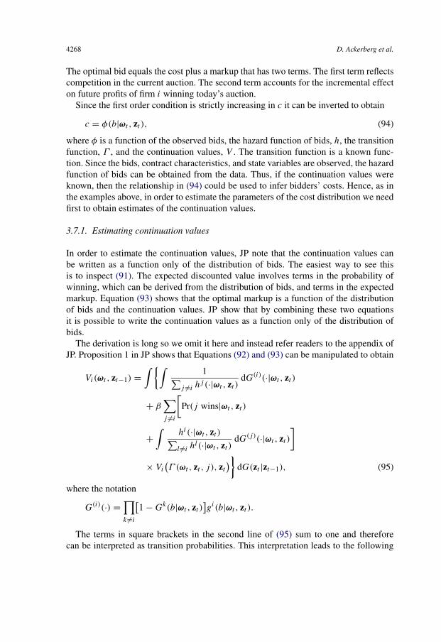
4268 D. Ackerberg et al.
The optimal bid equals the cost plus a markup that has two terms. The first term reflectscompetition in the current auction. The second term accounts for the incremental effecton future profits of firm i winning today’s auction.
Since the first order condition is strictly increasing in c it can be inverted to obtain
(94)c = φ(b|ωt , zt ),
where φ is a function of the observed bids, the hazard function of bids, h, the transitionfunction, Γ , and the continuation values, V . The transition function is a known func-tion. Since the bids, contract characteristics, and state variables are observed, the hazardfunction of bids can be obtained from the data. Thus, if the continuation values wereknown, then the relationship in (94) could be used to infer bidders’ costs. Hence, as inthe examples above, in order to estimate the parameters of the cost distribution we needfirst to obtain estimates of the continuation values.
3.7.1. Estimating continuation values
In order to estimate the continuation values, JP note that the continuation values canbe written as a function only of the distribution of bids. The easiest way to see thisis to inspect (91). The expected discounted value involves terms in the probability ofwinning, which can be derived from the distribution of bids, and terms in the expectedmarkup. Equation (93) shows that the optimal markup is a function of the distributionof bids and the continuation values. JP show that by combining these two equationsit is possible to write the continuation values as a function only of the distribution ofbids.
The derivation is long so we omit it here and instead refer readers to the appendix ofJP. Proposition 1 in JP shows that Equations (92) and (93) can be manipulated to obtain
Vi(ωt , zt−1) =∫ {∫
1∑j �=i hj (·|ωt , zt )
dG(i)(·|ωt , zt )
+ β∑j �=i
[Pr(j wins|ωt , zt )
+∫
hi(·|ωt , zt )∑l �=i hl(·|ωt , zt )
dG(j)(·|ωt , zt )
](95)× Vi
(Γ (ωt , zt , j ), zt
)}dG(zt |zt−1),
where the notation
G(i)(·) =∏k �=i
[1 − Gk(b|ωt , zt )
]gi(b|ωt , zt ).
The terms in square brackets in the second line of (95) sum to one and thereforecan be interpreted as transition probabilities. This interpretation leads to the following

Ch. 63: Econometric Tools for Analyzing Market Outcomes 4269
construction. Assume that the state space is discrete and let Ai be a vector with oneelement for each state representing the first term above
Ai(s) =∫∫
1∑j �=i hj (·|ωt , zt )
dG(i)(·|ωt , zt ) dG(zt |zt−1).
Next, construct the matrix Mi such that each element (k, l) reflects the transition prob-abilities above
Mik,l =
⎧⎪⎨⎪⎩[Pr(j wins|ωk, zl) + ∫ hi(·|ωk,zl )∑
l �=i hl (·|ωk,zl)dG(j)(·|ωk, zl)] Pr(zl |zk),
if ωl = Γ (ωk, zl, j),
0, otherwise.
Then the value function can be expressed as
(96)Vi = [I − βMi]−1
Ai.
The matrices Mi and Ai can be estimated using estimates of the bid distribution.
3.7.2. Estimating the cost distribution
Once the continuation values are known, estimating the cost distribution is straightfor-ward. There is a relationship between the cost distribution and the bid distribution thatis given by
F(c|ωt , zt ) = G(b(c,ωt , zt )
∣∣ωt , zt
) = G(φ−1(c|ωt , zt )
∣∣ωt , zt
)(provided that φ is invertible). The function φ can be estimated using the first ordercondition (93) and the estimated continuation values. The estimated φ can then be sub-stituted into the estimated bid distribution in order to obtain an estimate of the costdistribution.
3.8. Outstanding issues
The literature on structural estimation of dynamic games is relatively recent. As a resultour focus has been on reviewing assumptions and techniques that make it feasible touse the implications of dynamic games to make inferences on parameters of interest toI.O. We have paid little attention to a host of related issues including; the asymptoticefficiency of alternative estimators, the small sample properties of those estimators,identification in the absence of auxiliary information, and the likely validity of variousassumptions.
It is not our intention to minimize any of these issues. Indeed we think it important toexplore all of them, particularly the assumptions underlying the analysis. This includesthe behavioral assumptions and the assumptions regarding the selection of equilibria,as well as more traditional assumptions on the properties of the unobservables in themodel. The simple fact is that we have little to report on most of these issues. There

4270 D. Ackerberg et al.
is however one exception; problems that arise due to the presence of serially correlatedunobserved state variables. Since this is an issue that has appeared in several relatedliteratures, we do have some idea of how to deal with it in the context of estimatingdynamic games.
3.8.1. Serially correlated unobserved state variables
In all of the examples above it is assumed that all of the states that are commonly knownto the agents are also observed by the econometrician. In many empirical applicationsthis assumption is questionable. For example, in many cases we might expect there tobe an aggregate shock to profits that is known to all of the firms, but not controlledfor by the econometrician. The models presented above can be modified to accommo-date these shocks if they are i.i.d. over time. However we would often expect aggregateshocks to be serially correlated, just as most aggregate variables are. In that case, be-havior in previous periods would depend on previous realizations of the unobservedstates, leading to a correlation between today’s values of the observed and unobservedstates.
The statement of the problems caused by unobserved serially correlated state vari-ables in dynamic models with discrete outcomes dates back at least to Heckman (1981).Pakes (1994) reviews three possible solutions to the problem: (i) solving for the un-observed states as a function of observables, (ii) simulating the model from a trulyexogenous distribution of initial conditions, and (iii) using the ergodic distribution tomodel the long run relationship between the unobserved and observed states. With theadvent of longer panels there is also the possibility of using techniques that allow oneor more parameters to differ across markets in a panel of markets (say a market specifictime invariant profit parameter, or a separate initial condition for each market), and thenestimate those parameters pointwise.
The first case is quite promising in contexts where there is an observable continuousresponse to the unobservable state. Then conditional on the parameter vector, there isoften a one to one relationship between the unobserved states and the observed statesand controls. Several papers in the literature on static demand system estimation [Berry(1994), Berry, Levinsohn and Pakes (1995), and Bajari and Benkard (2005)] have usedsuch a condition to recover serially correlated unobserved product characteristics usingdata on quantities, prices, and observed product characteristics. Timmins (2002) uses asimilar procedure to control for the initial conditions in a single agent dynamic controlproblem with unobserved state variables. Olley and Pakes (1996) use the implicationsof a dynamic Markov perfect equilibrium model to recover a serially correlated produc-tivity term. These methods could be used to recover the unobserved state variables priorto the dynamic estimation, and then the unobserved state variables could be treated asif they were observed in the dynamic estimation algorithm (at least up to estimationerror).
Things become more difficult when the unobserved states are not recoverable in thisway. In single-agent dynamic models, several papers [e.g. Pakes (1986) and Keane and

Ch. 63: Econometric Tools for Analyzing Market Outcomes 4271
Wolpin (1997)] have used exogenous initial conditions to solve the problem of seriallycorrelated unobserved states. Starting with an exogenous initial distribution of states,the model can be used to simulate the relationship between the observed and unob-served states in future periods. However, while there may be many reasonable ways ofmodelling initial conditions for a single agent (be it a firm or an individual), such con-ditions tend to be less realistic for an industry, whose history is typically much longerthan the available data.
The third case is perhaps more appropriate for industry studies. Instead of using anexogenous initial condition for the unobserved states at the time the market starts up, weassume that the draws on the joint distribution of the unobserved states and the initialcondition are draws from an invariant distribution. That distribution is then estimatedalong with the other parameters of the problem. The rational here is that if the mar-kets in question have been in existence long enough, the joint distribution of the initialcondition and the unobserved state will not depend on the early years of the industry’sevolution. Rather it will depend only on the limiting structure of the Markov processgenerated by the nature of the dynamic game, a structure we can analyze.
Aguirregabiria and Mira (2007) implement one version of this solution. They allowfor an unobserved fixed effect which varies across markets and assume both that thefixed effect can only take on a finite number of values and that the transition probabilitiesfor the observed exogenous variables are independent of the values of the fixed effect.They then solve for an invariant distribution of the state of the system and the fixedeffect, form the conditional distribution of the initial condition given the fixed effect,and integrate out over possible values of the fixed effect. They report that allowing forthe fixed effect has a noticeable impact on their empirical results.
Of course, if one has a reasonably long panel of markets one should be able to esti-mate the fixed effect (or some other unobserved initial condition) pointwise; our fourthsolution possibility. In that case continuation values could be estimated as describedabove but separately for each market in the data. The observations across markets couldthen be pooled together in the second stage in order to estimate the structural parame-ters that are the same across markets. This would lead to substantially higher estimationerror in the continuation values, and one might want to think hard about estimators thatwould be designed to minimize the impact of these errors.62 Some Monte Carlo workon just how long a panel is likely to be required for this procedure to be fruitful wouldbe extremely helpful.
References
Abreu, D., Pearce, D., Stacchetti, E. (1986). “Optimal cartel equilibria with imperfect monitoring”. Journalof Economic Theory 39 (1), 251–259.
62 Note that this process could also solve the multiple equilibrium problem that might exist across markets.
4272 D. Ackerberg et al.
Ackerberg, D. (2003). “Advertising learning and customer choice in experience good markets: A structuralempirical examination”. International Economic Review 44 (3), 1007–1040.
Ackerberg, D., Pakes, A. (2005). “Notes on relaxing the scalar unobservable assumption in Olley and Pakes”.Mimeo. Harvard University.
Ackerberg, D., Caves, K., Fraser, G. (2004). “Structural identification of production functions”. Mimeo.UCLA.
Aguirregabiria, V., Mira, P. (2007). “Sequential estimation of dynamic games”. Econometrica 75 (1), 1–54.Ahn, H., Powell, J. (1993). “Semiparametric estimation of censored selection models with a nonparametric
selection mechanism”. Journal of Econometrics 58 (1–2), 3–29.Arellano, M., Bond, S. (1991). “Some tests of specification for panel data: Monte Carlo evidence and an
application to employment equations”. Review of Economic Studies 58, 277–297.Arellano, M., Bover, O. (1995). “Another look at the instrumental variable estimation of error-components
models”. Journal of Econometrics 68 (1), 29–51.Bajari, P., Benkard, C.L. (2005). “Demand estimation with heterogeneous consumers and unobserved product
characteristics: A hedonic approach”. Journal of Political Economy 113 (6), 1239–1276.Bajari, P., Benkard, C.L., Levin, J. (2007). “Estimating dynamic models of imperfect competition”. Econo-
metrica. In press.Benkard, C.L. (2000). “Learning and forgetting: The dynamics of aircraft production”. American Economic
Review 90 (4), 1034–1054.Benkard, C.L. (2004). “A dynamic analysis of the market for wide-bodied commercial aircraft”. Review of
Economic Studies 71 (3), 581–612.Berry, S. (1994). “Estimating discrete choice models of product differentiation”. RAND Journal of Eco-
nomics 25 (2), 242–262.Berry, S., Pakes, A. (2002). “Estimation from the optimality conditions for dynamic controls”. Mimeo. Yale
University.Berry, S., Pakes, A. (2005). “The pure characteristics demand model”. Mimeo. Yale University.Berry, S., Levinsohn, J., Pakes, A. (1995). “Automobile prices in market equilibrium”. Econometrica 63 (4),
841–890.Berry, S., Levinsohn, J., Pakes, A. (1999). “Voluntary export restraints on automobiles: Evaluating a trade
policy”. American Economic Review 89 (3), 400–430.Berry, S., Levinsohn, J., Pakes, A. (2004). “Estimating differentiated product demand systems from a combi-
nation of micro and macro data: The new car model”. Journal of Political Economy 112 (1), 68–105.Berry, S., Linton, O., Pakes, A. (2004). “Limit theorems for estimating the parameters of differentiated prod-
uct demand systems”. Review of Economics Studies 71 (3), 613–654.Blundell, R., Bond, S. (1999). “GMM estimation with persistent panel data: An application to production
functions”. Working Paper Series No. W99/4. The Institute for Fiscal Studies.Bond, S., Söderbom, M. (2005). “Adjustment costs and the identification of Cobb Douglas production func-
tions”. Institute for Fiscal Studies WP O5/04.Bresnahan, T. (1981). “Departures from marginal-cost pricing in the American automobile industry: Estimates
for 1977–1978”. Journal of Econometrics 17 (2), 201–227.Bresnahan, T. (1982). “The oligopoly solution concept is identified”. Economics Letters 10, 87–92.Bresnahan, T. (1987). “Competition and collusion in the American automobile industry: The 1955 price war”.
Journal of Industrial Economics 35 (4), 457–482.Buettner, T. (2004a). “Productivity dynamics when labor is a state variable”. Mimeo. LSE.Buettner, T. (2004b). “R&D and the dynamics of productivity”. Mimeo. LSE.Caballero, R., Engel, E.M.R.A. (1999). “Explaining investment dynamics in US manufacturing: A generalized
(S, s) approach”. Econometrica 67 (4), 783–826.Chamberlain, G. (1984). “Panel data”. In: Arrow, K., Intriligator, M. (Eds.), Handbook of Econometrics,
vol. 2. Elsevier Science, pp. 1247–1318. Chapter 22.Chan, T. (2002). “Demand for soft drinks: Characteristics, corners and continuous choice”. Mimeo. Washing-
ton University, Marketing Department.

Ch. 63: Econometric Tools for Analyzing Market Outcomes 4273
Chernozhukov, V., Hong, H., Tamer, E. (2007). “Estimation and confidence regions for parameter sets ineconomic models”. Econometrica. In press.
Court, A. (1939). “Hedonic price indexes with automotive examples”. In: The Dynamics of AutomobileDemand. General Motors Corporation, Detroit, pp. 99–117.
Crawford, G., Shum, M. (2007). “Uncertainty and learning in pharmaceutical demand”. Econometrica 73 (4),1137–1173.
Das, M., Olley, G.S., Pakes, A. (1996). “The evolution of the market for consumer electronics”. Mimeo.Harvard University.
Davis, S., Haltiwanger, J. (1992). “Gross job creation, gross job destruction, and employment reallocation”.Quarterly Journal of Economics 107 (2), 819–864.
Deaton, A., Muellbauer, J. (1980). “An almost ideal demand system”. American Economic Review 70 (3),312–326.
Department of Justice. (1992). “US Merger guidelines”.Doraszelski, U., Judd, K. (2004). “Solution methods for Markov perfect Nash equilibria of continuous time,
finite state stochastic games”. Mimeo. Hoover Institution.Doraszelski, U., Markovich, S. (2007). “Advertising dynamics and competitive advantage”. RAND Journal
of Economics. In press.Doraszelski, U., Pakes, A. (2007). “A framework for applied dynamic analysis in I.O.” In: Armstrong, M.,
Porter, R. (Eds.), Handbook of Industrial Organization, vol. 3. North-Holland, Amsterdam. In press.Doraszelski, U., Satterthwaite, M. (2007). “Foundations of Markov-perfect industry dynamics: Existence,
purification, and multiplicity”. Mimeo. Hoover Institution.Dubin, J., McFadden, D. (1984). “An econometric analysis of residential electric appliance holdings and
consumption”. Econometrica 52 (2), 345–362.Dunne, T., Roberts, M., Samuelson, L. (1988). “Patterns of firm entry and exit in US manufacturing indus-
tries”. RAND Journal of Economics 19 (4), 495–515.Dunne, T., Klimek, S., Roberts, M., Xu, Y. (2006). “Entry and exit in geographic markets”. Mimeo. Pennsyl-
vania State University.Einav, L. (2003). “Not all rivals look alike: Estimating an equilibrium model of the release date timing game”.
Mimeo. Stanford University.Erdem, T., Keane, M. (1996). “Decision-making under uncertainty: Capturing dynamic brand choice
processes in turbulent consumer goods markets”. Marketing Science 15 (1), 1–20.Erdem, T., Imai, S., Keane, M. (2003). “Brand and quantity choice dynamics under price uncertainty”. Quan-
titative Marketing and Economics 1 (1), 5–64.Ericson, R., Pakes, A. (1995). “Markov-perfect industry dynamics: A framework for empirical work”. Review
of Economic Studies 62 (1), 53–83.Esteban, S., Shum, M. (2002). “Durable good monopoly with secondary markets: The case of automobiles”.
Mimeo. Johns Hopkins.Fershtman, C., Pakes, A. (2000). “A dynamic oligopoly with collusion and price wars”. RAND Journal of
Economics 31 (2), 207–236.Fershtman, C., Pakes, A. (2005). “Finite state dynamic games with asymmetric information: A computational
framework”. Mimeo. Harvard University.Gentzkow, M. (2004). “Valuing new goods in a model with complementarity: Online newspapers”. Mimeo.
Chicago GSB.Gorman, W. (1959). “Separable utility and aggregation”. Econometrica 27, 469–481.Gowrisankaran, G. (1995). “A dynamic analysis of mergers”. PhD dissertation, Department of Economics,
Yale University.Gowrisankaran, G., Town, R. (1997). “Dynamic equilibrium in the hospital industry”. Journal of Economics
and Management Strategy 6 (1), 45–74.Green, E., Porter, R. (1984). “Non-cooperative collusion under imperfect price information”. Economet-
rica 52, 87–100.Greenstreet, D. (2005). “Exploiting sequential learning to estimate establishment-level productivity dynamics
and decision rules”. Mimeo. University of Michigan.

4274 D. Ackerberg et al.
Griliches, Z. (1961). “Hedonic price indexes for automobiles: An econometric analysis of quality change”.In: The Price Statistics of the Federal Government. NBER, New York.
Griliches, Z., Hausman, J. (1986). “Errors in variables in panel data”. Journal of Econometrics 31 (1), 93–118.Gronau, R. (1974). “Wage comparisons – A selectivity bias”. Journal of Political Economy 82 (6), 1119–1143.Guerre, E., Perrigne, I., Vuong, Q. (2000). “Optimal nonparametric estimation of first-price auctions”. Econo-
metrica 68 (3), 525–574.Hansen, L. (1982). “Large sample properties of generalized method of moments estimators”. Econometrica 50
(4), 1029–1054.Hausman, J. (1996). “Valuation of new goods under perfect and imperfect competition”. In: Bresnahan, T.,
Gordon, R. (Eds.), The Economics of New Goods. University of Chicago Press, Chicago, pp. 209–248.Chapter 5.
Heckman, J. (1974). “Shadow prices, market wages, and labor supply”. Econometrica 42 (4), 679–694.Heckman, J. (1976). “The common structure of statistical models of truncation, sample selection and limited
dependent variables and a simple estimator for such models”. Annals of Economic and Social Measure-ment 5 (4), 475–492.
Heckman, J. (1978). “Dummy endogenous variables in a simultaneous equation system”. Econometrica 46(4), 931–959.
Heckman, J. (1979). “Sample selection bias as a specification error”. Econometrica 47 (1), 153–161.Heckman, J. (1981). “The incidental parameters problem and the problem of initial conditions in estimating a
discrete time discrete data stochastic process”. In: Manski, C., McFadden, D. (Eds.), Structural Analysisof Discrete Data and Econometric Applications. MIT press. Chapter 4.
Heckman, J., Honoré, B. (1990). “The empirical content of the roy model”. Econometrica 58, 1121–1149.Heckman, J., Robb, R. (1985). “Alternative methods for evaluating the impact of interventions: An overview”.
Journal of Econometrics 30 (1–2), 239–267.Heckman, J., Snyder, J.M. (1997). “Linear probability models of the demand for attributes with an empirical
application to estimating the preferences of legislators”. RAND Journal of Economics 28 (0), S142–S189.Hendel, I. (1999). “Estimating multiple-discrete choice models: An application to computerization returns”.
Review of Economic Studies 66 (2), 423–446.Hendel, I., Nevo, A. (2002). “Sales and consumer inventory”. NBER working paper #9048.Hoch, I. (1962). “Estimation of production parameters combining time-series and cross-section data”. Econo-
metrica 30 (1), 34–53.Houthakker, H.S. (1955). “The Pareto distribution and the Cobb–Douglas production function”. Review of
Economic Studies 23 (1), 27–31.Hotelling, H. (1929). “Stability in competition”. Economic Journal 39, 41–57.Hotz, V., Miller, R. (1993). “Conditional choice probabilities and the estimation of dynamic models”. Review
of Economic Studies 60 (3), 497–529.Hotz, V., Miller, R., Sanders, S., Smith, J. (1994). “A simulation estimator for dynamic models of discrete
choice”. Review of Economic Studies 60, 397–429.Imbens, G., Lancaster, T. (1994). “Combining micro and macro data in microeconometric models”. Review
of Economic Studies 61 (4), 655–680.Jofre-Bonet, M., Pesendorfer, M. (2003). “Estimation of a dynamic auction game”. Econometrica 71 (5),
1443–1489.Keane, M., Wolpin, K. (1997). “The career decisions of young men”. Journal of Political Economy 105 (3),
473–522.Lancaster, K. (1971). Consumer Demand: A New Approach. Columbia University Press, New York.Lau, L.J. (1982). “On identifying the degree of competitiveness from industry price and output data”. Eco-
nomics Letters 10, 93–99.Levinsohn, J., Petrin, A. (2003). “Estimating production functions using inputs to control for unobservables”.
Review of Economic Studies 70 (2), 317–341.Magnac, T., Thesmar, D. (2002). “Identifying dynamic discrete decision processes”. Econometrica 70 (2),
801–816.

Ch. 63: Econometric Tools for Analyzing Market Outcomes 4275
Manski, C., Lerman, S. (1977). “The estimation of choice probabilities from choice based samples”. Econo-metrica 45 (8), 1977–1988.
Marschak, J., Andrews, W.H. (1944). “Random simultaneous equations and the theory of production”. Econo-metrica 12 (3–4), 143–205.
McFadden, D. (1974). “Conditional logit analysis of qualitative choice behavior”. In: Zarembka, P. (Ed.),Frontiers of Econometrics. Academic Press, New York.
McFadden, D. (1981). “Econometric models of probabilistic choice”. In: Manski, C., McFadden, D. (Eds.),Structural Analysis of Discrete Data with Econometric Applications. MIT Press, Cambridge, MA.
Mundlak, Y. (1961). “Empirical production function free of management bias”. Journal of Farm Economics 43(1), 44–56.
Nadiri, M.I., Rosen, S. (1974). A Disequilibrium Model of Demand for Factors of Production. National Bu-reau of Economic Research, New York.
Nevo, A. (2001). “Measuring market power in the ready-to-eat cereal industry”. Econometrica 69 (2), 307–342.
Olley, G.S., Pakes, A. (1996). “The dynamics of productivity in the telecommunications equipment industry”.Econometrica 64 (6), 1263–1298.
Pakes, A. (1986). “Patents as options: Some estimates of the value of holding European patent stocks”. Econo-metrica 54, 755–784.
Pakes, A. (1994). “The estimation of dynamic structural models: Problems and prospects, part II. Mixedcontinuous-discrete control models and market interactions”. In: Laffont, J.J., Sims, C. (Eds.), Advancesin Econometrics: Proceedings of the 6th World Congress of the Econometric Society. Cambridge Univ.Press. Chapter 5.
Pakes, A. (1995). “Biases in the CPI”. Testimony before the Senate Finance Committee, the United StatesCongress.
Pakes, A. (1998). “A framework for dynamic analysis in applied I.O.”. NBER discussion paper No. 8024.Pakes, A. (2004). “Common sense and simplicity in industrial organization”. Review of Industrial Organiza-
tion 23, 193–215.Pakes, A., Griliches, Z. (1984). “Estimating distributed lags in short panels with an application to the specifi-
cation of depreciation patterns and capital stock constructs”. Review of Economic Studies 51, 243–262.Pakes, A., McGuire, P. (1994). “Computing Markov-perfect Nash equilibria: Numerical implications of a
dynamic differentiated product model”. RAND Journal of Economics 25 (4), 555–589.Pakes, A., McGuire, P. (2001). “Stochastic approximation for dynamic models: Markov perfect equilibrium
and the ‘Curse’ of dimensionality”. Econometrica 69 (5), 1261–1281.Pakes, A., Olley, G.S. (1995). “A limit theorem for a smooth class of semiparametric estimators”. Journal of
Econometrics 65 (1), 295–332.Pakes, A., Pollard, D. (1989). “Simulation and the asymptotics of optimization estimators”. Econometrica 57
(5), 1027–1057.Pakes, A., Ostrovsky, M., Berry, S. (2007). “Simple estimators for the parameters of discrete dynamic games
(with entry/exit examples)”. RAND Journal of Economics. In press.Pakes, A., Porter, J., Ho, K., Ishii, J. (2006). “Moment inequalities and their application”. Mimeo. Harvard
University.Pavcnik, N. (2002). “Trade liberalization, exit, and productivity improvements: Evidence from Chilean
plants”. Review of Economic Studies 69, 245–276.Pesendorfer, M., Schmidt-Dengler, P. (2003). “Identification and estimation of dynamic games”. NBER work-
ing paper #9726.Petrin, A. (2002). “Quantifying the benefits of new products: The case of the minivan”. Journal of Political
Economy 110 (4), 705–729.Robinson, P. (1988). “Root-N-consistent semiparametric regression”. Econometrica 56 (4), 931–954.Rosenbaum, P., Rubin, D. (1983). “The central role of the propensity score in observational studies for causal
effects”. Biometrika 70 (1), 41–55.Rotemberg, J., Saloner, G. (1985). “A supergame-theoretic model of business cycles and price wars during
booms”. American Economic Review 76, 390–407.

4276 D. Ackerberg et al.
Rubinstein, R. (1981). Simulation and the Monte Carlo Method. John Wiley and Sons, New York.Rust, J. (1987). “Optimal replacement of GMC bus engines”. Econometrica 55, 999–1033.Rust, J. (1994). “Structural estimation of Markov decision processes”. In: Engle, R.F., McFadden, D.L. (Eds.),
Handbook of Econometrics, vol. IV. Elsevier Science, Amsterdam.Ryan, S. (2006). “The costs of environmental regulation in a concentrated industry”. Mimeo. Duke University.Salop, S. (1979). “Monopolistic competition with outside goods”. RAND Journal of Economics 10 (1), 141–
156.Shaked, A., Sutton, J. (1982). “Relaxing price competition through product differentiation”. Review of Eco-
nomic Studies 49 (1), 3–13.Schmidt-Dengler, P. (2003). “The timing of new technology adoption: The case of MRI”. Mimeo. Yale Uni-
versity.Sobel, J. (1984). “The timing of sales”. Review of Economic Studies 51 (3), 353–368.Song, M. (2004). “Measuring consumer welfare in the CPU market: An application of the pure characteristics
demand model”. Mimeo. Georgia Tech.Timmins, C. (2002). “Measuring the dynamic efficiency costs of regulators’ preferences: Municipal water
utilities in the arid west”. Econometrica 70 (2), 603–629.Train, K. (2003). Discrete Choice Models with Simulation. Cambridge University Press.Weintraub, G., Benkard, C.L., Van Roy, B. (2007). “Markov perfect industry dynamics with many firms”.
Mimeo. Stanford University.Wooldridge, J. (2002). Econometric Analysis of Cross Section and Panel Data. MIT Press, Cambridge, MA.Wooldridge, J. (2004). “On estimating firm-level production functions using proxy variables to control for
unobservables”. Mimeo. Michigan State University.