Econometric approach for Basel III Loss Given Default Estimation:

from discount rate to final multivariate model

Stefano Bonini1 – Giuliana Caivano2

Abstract: LGD – defined as credit loss when extreme events occur influencing the obligor

ability to repay debts - has a high relevance into credit and recovery process because of its

direct impact on capital savings, as stressed by the new Regulatory changes. This paper finds

out that most part of research on recoveries determinants are focused on Bond US Market and

few studies have been done on real lending portfolios from European Commercial Banks. Our

study contributes to the strand of the literature studying the determinants of recovery rates

through a linear regressive multivariate model on 10 years of historical workout real data of

Corporate and Retail loans from a panel of European Commercial Banks supervised by ECB.

The reliability of results is verified through the Accuracy Ratio. Finally, this paper provides a

useful benchmark analysis on different approaches for discounting cash flows given the

Regulatory evolutions on this topic.

Keywords: Loss Given Default, Rating Model, Basel2, Credit Risk Modeling, Quantitative

Finance.

JEL Reference: C13, C18, C51, C52, C53, G21

1University of Bologna, Piazza Scaravilli 2 – 40126 - Bologna (Italy) – stefano.bonini@unibo.it - PRESENTER 2 University of Bologna, Piazza Scaravilli 2 – 40126 - Bologna (Italy) - giuliana.caivano@unibo.it

1. Introduction

Today, even because of the amount of Non Performing Loans that arise from the crisis years,

Financial Institutions across Europe need more and more reliable and usable risk management

tools that are continuily evolvolving under the regulatory framework (as in European Union

(2013), European Banking Authority (2016) and European Central Bank (2017)). According to

them, the use of advanced internal rating based approaches are the best way to enlarge the risk

culture into the entire banking and credit processes. In this panorama the Loss Given Default

(LGD) Models have a high relevance, given the direct impact of LGDs into credit and recovery

process because of its direct impact on capital savings.

The existing literature on LGD is for the most part related to US market of Corporate Bonds

given the public availability of data thus in most cases the existing papers try to test different

statistical approaches applying them on external data (e.g. recoveries data from Rating

Agencies). Given the relevance of LGD in capital requirements calculation, it is very important

for banks, bankers, Regulators and academics to understand that depending on the methodology

chosen, results can lead to different estimated values and different drivers combination. Our

paper can contribute to the strand of the literature studying the determinants of recovery rates

identifying the real recovery drivers on Corporate and Retail loans under the new Credit Risk

Regulatory environment. For our study we have used a large panel dataset comprising 26,000

defaulted loans from 2005 to 2015 coming from different Italian banks under the European

Central Bank Supervision and belonging to Corporate and Retail segments of client. We have

applied different approaches for discounting cash flows, confirming the goodness of Capital

Asset Pricing Model for spread estimation. Finally, the best recoveries determinants have been

identified by a linear regression multivariate approach based on an ordinary least squares

parameters estimation.

This study also provides a comparative analysis among different ways of defining discount rate,

also in the light of the recent enphasis of Regulator (as in European Banking Authority (2016))

on the approach used to discount cash flows, finally choosing CAPM for discounting cash flows

on the portfolio used for the application. This paper is very important since very few analyses on

recovery rates of bank loans are focused on continental Europe Banking market, having found

that the most part of research on recoveries are focused on Bond US Market.

2. Literature Review

As previously mentioned, most empirical research of the last 10 years focuses on modeling and

estimating the determinants of recoveries on US Market of Corporate Defaulted Bonds and only

few studies on recoveries or lossess on loans from European countries are available from

researchers and pratictioners.

I. Approaches for identifying modeling approach and recovery drivers

One of the first studies aimed to identify a possible framework defining the best determinants of

recoveries is the one of Shuermann (2004), in which the author tries to define a possible set of

statistical techniques to be used for developing LGD and depending on the level of knowledge each

bank has about this risk parameter. In particular, the author identifies look-up tables as an easy way

to compute LGD by producing single cells of values (a cell for example might be LGD for

subordinated loans belonging to automotive industry during a recession). Another way to estimate

LGDs could be the use of basic regressions (with a medium level of sophistication) in which all

variables are treated as dummies of only one regression (for example dummies for Senior/Junior

loans, collateral type, industry group, expansion / recession). A medium – high sophisticate

approach is to use advanced regressions, in which each dummy variable can be treated as part of a

specific regression. The author identifies also some most complicated approaches as neural net,

decision trees, machine learning. Starting from this work, other authors have tried to compare

different approaches for developing LGD model.

Araten et al. (2004) try to investigate the role of collaterals in explaining recovery rates analyzing

18 years of loan loss history at JPMC for 3,761 defaulted borrowers. Using a look-up table

methodology and testing the following variables as main drivers: business unit, industry group,

geographic region, cohort year, and collateral type. They find that economic LGD on unsecured

loans is expected to be higher. They also try to test the link between LGDs and business cycle,

observing that LGDs for unsecured loans exhibit relatively high correlation with the economic

cycle.

Gupton (2005) tests LossCalc model (Moody’s KMV) to predict loss given default, applying

multiple predictive factors at different information levels: collateral, instrument, firm, industry,

country and the macroeconomic scenarios to predict LGD. Data used is represented by a global

dataset of 3,026 recovery observations for loans, bonds and preferred stock from 1981 to 2004. He

finds that recovery rates worldwide are predictable within a common statistical framework, which

suggests that the estimation of economic firm value is a dominant step in LGD determination.

Sabato et al. (2005) analyze the link between recoveries and the credit cycle for retail assets, to

investigate the issue of estimating conservative LGD for retail exposures and to propose a solution

for the common lack of retail recoveries data to cover a full credit cycle (including an economic

downturn). They calculate LGD using ultimate recoveries observed one year after the default event

and we analyze them at regulatory asset class level: the adverse dependencies between default rates

and recovery rates are not present in all asset classes. They also propose two different techniques

for secured and unsecured exposures. For the former, they stress the value of the collateral and the

cure rate in order to find the expected increase of the LGD in a downturn period. For the latter

instead, they use the existing correlation between default rates and recovery rates, if any, to quantify

the amount of conservatism to be added to the LGD during a period of default rates significantly

higher than the mean (i.e., downturn period).

Dermine et al. (2006), starting from Dermine et al. (2004), try to investigate the role of guarantees

and collaterals in explaining the link between cumulative recovery rates and dynamic provisions.

Using a log-log regression applied to the same sample used in their previous study, they find that

bad and doubtful loans with no guarantee/collateral exhibit better recoveries than loans with

personal guarantee (this could be due to the fact that the decision to lend without guarantee took

into account the higher expected recovery rates). They also find that the past recovery history has a

highly significant positive impact on future recovery and finally, a comparison with the Bank of

Portugal mandatory provisioning rules indicates some regulatory conservatism in calling for 100%

provision 31 months after the default date, when, in fact, significant amounts are still recovered

after that date.

Altman et al. (2008) present a detailed review of approaches for credit risk models, developed

during the last thirty years, treat the recovery rate and, more specifically, its relationship with the

probability of default of an obligor. They also review the efforts by rating agencies to formally

incorporate recovery ratings into their assessment of corporate loan and bond credit risk and the

recent efforts by the Basel Committee on Banking Supervision to consider “downturn LGD” in their

suggested requirements under Basel II. Their literature review shows that there are recent empirical

evidence concerning these issues and the latest data on high-yield bond and leverage loan defaults

are also presented and discussed.

Caselli et al. (2008) verify the existence of a relation between loss given default rate (LGDR) and

macroeconomic conditions on an Italian portfolio of bank loans by using both logistic and linear

regression models. The authors pinpoint different macroeconomic explanatory variables for LGDR

on loans to households and SMEs. For households, LGDR is more sensitive to the default-to-loan

ratio, the unemployment rate, and household consumption. For SMEs, LGDR is influenced by the

total number of employed people and the GDP growth rate.

Acharya et al. (2008) show that creditors of defaulted firms recover significantly lower amounts in

present-value terms when the industry of defaulted firms is in distress. The authors use data on

defaulted firms in the United States over the period 1982–1999 and test it through a linear

regression model using contract-specific characteristics (seniority and presence of collateral),

industry of defaulting firm (utility sector or other sector), and macroeconomic condition (aggregate

default intensity).

Couwenberg et al. (2008) test the relationship between Dutch bankruptcy law system (that is a

liquidation-based system) and firm recovery rates by using data from files of bankrupt companies in

The Netherlands and collecting all information about process of resolving financial distress (time

taken for asset sales to complete, type of buyer, managerial involvement, employees laid off,

involvement of prior lenders, length of automatic stay, conflicting rights on assets, procedures

started and resolution of the bankruptcy procedure) and on the pay-out on all the debts. Using a

linear regression, the authors find that the firm recovery rate is higher when firms have more fixed

assets, a higher quick ratio, are not liquidated and continue their operations in bankruptcy.

Davydenko et al. (2008) study the effects of bankruptcy codes in France, Germany, and the United

Kingdom on recovery rates of defaulted firms. The authors apply linear regressions to a unique data

set of small to-medium size almost privately owned, defaulted on their bank debt. The data include

detailed information on the terms of the loan contracts, the event of default and its resolution (either

bankruptcy or workout), collateral values and the proceeds from asset sales, and banks’ recovery

rates. The authors observe that collateral requirements at loan origination directly reflect the bank’s

ability to realize assets upon default. Thus, because the proceeds from collateral sales are lower in

France, at loan origination French banks demand higher levels of collateral per dollar of debt.

Moreover, the composition of different types of collateral reflects their expected value in default.

Chalupa et al. (2009) apply different statistical techniques (classic linear regression models, models

with fractional responses and models with ordinal responses) to a set of firm loan micro-data of an

anonymous Czech commercial bank in order to test empirically the determinants of LGDs. They

find that LGD is driven primarily by the period of loan origination, relative value of collateral, loan

size and length of business relationship. They also find that in more complex models, log-log

models appear to perform better, implying an asymmetric response of the dependent variable.

Bastos (2010) tries to test on a Portuguese sample of 347 loans two methodologies: linear

regression and decision tree, with the following variables as drivers: loan amount, presence and

amount of collateral, sector of activity, interest rate, rating, duration of loan. The results show a

higher predictive power of decision tree.

Witzany et al. (2010) propose an application of the survival time analysis methodology to

estimations of the Loss Given Default (LGD) parameter. The authors identify a main advantage of

the survival analysis approach compared to classical regression methods that is the possibility of

exploiting partial recovery data. The empirical tests performed show that the Cox proportional

model applied to LGD modeling performs better than the linear and logistic regressions.

Yashkir et al. (2012) investigate several of the most popular loss given default (LGD) models (least-

squares method, Tobit, three-tiered Tobit, beta regression, inflated beta regression, censored gamma

regression) in order to compare their performance. They show that for a given input data set the

quality of the model calibration depends mainly on the proper choice (and availability) of

explanatory variables (model factors), but not on the fitting model. Model factors have been chosen

based on the amplitude of their correlation with historical LGDs of the calibration data set.

Numerical values of non-quantitative parameters (industry, ranking, type of collateral) are

introduced as their LGD average. They show that different debt instruments depend on different

sets of model factors (from three factors for revolving credit or for subordinated bonds to eight

factors for senior secured bonds).

Yang et al. (2012) apply different statistical techniques (mainly the ones described by Schuermann)

on a real portfolio of commercial loans by using the following information as drivers: borrower

level utilization, facility level of collateralization, facility authorized amount, ratio of limit increase

to undrawn, total assets value, industry code, facility level utilization, total facility collateral

percentage value. The authors perform a comparison in accuracy power of the applied techniques,

showing that Naïve Bayes methods have a lower R-square (26%) if compared to logit models (27%)

or neural network (35%).

Thomas et al. (2012) try to investigate what are the main drivers of LGDs under two different

collection policies: “In house” and “third part”. The authors apply different statistical techniques on

two different samples: the first one, related to in house collection procedures, is represented by

11,000 defaulted consumer loans defaulted over a two-year period in the 1990s; the second one,

concerning third part collection policies, is given by 70,000 loans where the outstanding debts

varied from £10 to £40,000. They try to apply different statistical techniques on the two samples, by

obtaining a higher predictive power of all models applied (linear regressions, Box Cox, Beta

distribution, Log Normal transformation, WOE approach) on sample related to in house procedures.

Bonini et al. (2013) apply survival analysis techniques on a sample of Italian Retail Loans portfolio

in estimating danger rate correction factor for computation of LGDs on doubtful loans. The authors

take into account this statistical methodology above all because the censoring phenomenon ensures

consistent forecasting independent from the size of the credit loan portfolio. The variables

considered for their analysis are mainly related to the kind of employer, by detecting a R-square of

more than 75%. In another work (2014) the authors apply the credibility theory in order to estimate

LGD values embedding the quality level of credit risk mitigators.

Frontczack et al. (2015) addresses to the appropriate modeling of loss given default (LGD) for the

retail business sector assuming small or mid-size loans that are assigned in a standardized way and

collateralized by residential or commercial property. They choice an exponential Ornstein–

Uhlenbeck diffusion as the stochastic process of the collateral combines the desirable features with

the charm of analytical solvability which seems to be of advantage as regards acceptance among

practitioners.

Miller et al. (2017) analyse the determinant of recoveries on leasing portfolio, distinguishing

between asset-related and miscellaneous revenues of the workout process in order to calculate

component LGDs. They introduce a multi-step approach to estimate the overall LGD of leases,

based on its economic composition obtaining valuable information regarding the debt collection

procedure that lead to monetary advantages for the lessor.

Finally, Hwang et al. (2017) propose to estimate the loss given default (LGD) first applying the

logistic regression to estimate the LGD cumulative distribution function. Then, they convert the

result into the LGD distribution estimate. They have assessed the results on a sample of 5269

defaulted debts from Moody’s Default and Recovery Database.

The literature review on this topic has highlighted that also if there are statistical techniques

ensuring a higher predictive power (decision trees as in Bastos (2009)), it is not possible to define

which is the best methodology because the choice can be affected both by bank knowledge (as in

Shuermann (2004)) and data availability as in Khieu et al. (2012) and Qi et al. (2012).

The literature review has been also highlighted that the best determinants of recoveries on loans

portfolios of Corporate and Retail clients are related to loan attributes as amount (Dermine et al.

(2006), Chalupa et al. (2008), Grunert et al. (2009) and Gurtler et al. (2009)), kind of credit risk

mitigators covering the loan (Bastos (2009) and Araten et al. (2004)), collateral amount (Yang et al.

2012, Grunert et al. (2009) and Leow et al. (2012)) and duration of default (Araten et al. (2004),

Chalupa et al. (2008) and Carty et al. (2000)), but also the attributes of client, such as the rating

(Bastos 2009), age of corporate (Bastos (2009) and Chalupa et al. (2008)), duration of loan

(Dermine et al. (2006) and Bastos (2009)) and industry sector (Araten et al. (2004), Dermine et al.

(2006) and Bastos (2009)).

Following these findings, we will try to identify the best combination of variables in predicting

recovery rates through OLS regression.

II. Approaches for identifying discount rate

It can be remarked that for the estimation of LGD, Regulators requires that “The measures of

recovery rates used in estimating LGDs should reflect the cost of holding defaulted assets over the

workout period, including an appropriate risk premium. (….) In establishing appropriate risk

premiums for the estimation of LGDs consistent with economic downturn conditions, the institution

should focus on the uncertainties in recovery cash flows associated with defaults that arise during

an economic downturn…(…)”.3

In addition, the recent evolutions on Credit Risk Modeling – as in European Banking Authority

(2016) highlights how choosing the appropriate discount with contractual rate or funding rate could

not really aligned with Regulatory requirements, supporting the choice of a discount rate based on a

risk-free rate and a spread.

Cost of funding is studied in Yang et al. 2008, using 1 year Libor (plus a spred of 3%) for

discounting cash flows coming from mortgages with high Loan to Value, considering this rate much

more useful for reflecting the recoveries uncertainty and the presence of an undiversifiable risk

component. For what concernes the return of defaulted bonds (the market price of bonds after issuer

default), Jacobs et al. 2010 calculate discount rate as the annual return of defaulted bonds between

the opening and closing of default event through the application of a maximum-likehood function

starting from the pricing normalized error. Other authors, as Brady et al. 2006 adopt a regressive

approach for modeling discount rate on defaulted bonds based on their market price and sector

dummies. The use of loan interest rate can be found in Bastos 2009 applied to a Portuguese bank

portfolio. The author highlights that there is no substantial difference in discounted recoveries

considering a fixed discount rate not changing over time. Also Dermine et al. 2005 adopt a loan

3 Bank of Italy: Nuove disposizioni di vigilanza prudenziale per le banche. Circolare n. 263, Titolo II, Capitolo 1

interest rate, but they discover that the outstanding capital could be different from the loan amount

at the moment of default because of the absence of an adequate risk premium. For Gürtler et al.

2013 the loan interest rate is an approach approved by Regulators. Other authors, as Araten et al.

2004 adopt a “vulture” rate opposite to the loan interest rate or cost of funding, because it is

considered much more reflecting the riskness of defaulted cash flows.

Altman et al. 2005 study the adoption of risk-free rate analyzing historical time series on American

defaulted Bonds, considering this rate able to reflect to volatility of defaulted Bonds implied

returns.

Finally, Machlahan 2005 assumes that cash flows observed after the default can be a proxy of

financial assets. Based on this assumption, he says that the best discount rate must take into account

also a systematic risk component acting on assets after default and he applies the framework of

Capital Asset Pricing Model (Sharpe 1994). Also Gibilaro et al. 2007 evaluate the estimation of a

risk premium component (in addition to the risk – free rate) through the estimation of a

monofactorial rate based on market index or macroeconomic variables. In 2011 they try to evolve

their model estimating a multifactorial rate obtaining LGDs with a low volatility. Also Witzany et

al. 2009 and Subarna 2013 apply CAPM for defining discount rate and they introduce the

correlation factor deriving from the Basel 2 risk-weights functions for calculating β. Finally,

Chalupa et al. 2008 apply CAPM framework defining different risk premium according to the type

of collateral covering the portfolio.

Here we show our considerations on each approach analyzed aimed to justify and reinforce the

choice of CAPM model:

Contractual loan doesn’t make possible a diversification of returns pre and post default (it is

not so common a frequent negotiation of contractual conditions during the whole life of a

loan, maybe except for mortgages);

The adoption of the only risk-free rate is subject to the identification of the reference market;

The adoption of funding cost is based on the assumption that systemic risk of defaulted asset

replaces the risk of bank;

Ex-post Defaulted Bonds returns are influenced by the volatility embedded in the chosen

index.

In addition to these considerations, in order to choose the best discount rate to be applied to our

data, we have compared the results deriving from the adoption of a CAPM spread with the

outcomes deriving from the use of a discount factor based only on risk-free rate or using internal

spreads / funding rates. We have found that recovery rates based on discounted cash flows

adopting a risk –free rate added to a spread derived from CAPM are less volatiles (given an

average value not so different with what can be obtained adopting the other proposed

approaches).

In this paper we have applied and compared three different approaches for discounting cash

flows for Economic Loss Given Default calculation: contractual loan rate, risk-free rate and risk-

free rate plus a spread derived from CAPM. We have found that the adoption of a risk-free rate

plus a spread ensure a lower volatility of LGDs and in the same time a higher conservatism of

estimates.

3. Methodological Framework

3.1 Workout LGD calculation

The best practice on European Banks, in particular on Retail Portfolios, is to use a workout

approach for estimating Recovery Rates. Infact the same CEBS Guidelines4 specifies that: “LGD

estimates based on an institution’s own loss and recovery experience should in principal be

superior to other types of estimates, all other things being equal, as they are likely to be most

representative of future outcomes”. (….) “The market and implied market LGD techniques can

currently be used only in limited circumstances. They may be suitable where capital markets are

deep and liquid. It is unlikely that any use of market LGD can be made for the bulk of the loan

portfolio”. (…) “The implied historical LGD technique is allowed only for the Retail exposure

class (…). The estimation of implied historical LGD is accepted in case where institutions can

estimate the expected loss for every facility rating grade or pool of exposures, but only if all the

minimum requirements for estimation of PD are met .

The workout LGD estimation is based on economic notion of loss including all the relevant costs

tied to the collection process, but also the effect deriving from the discount of cash flows, as

required by CEBS Guidelines:“The measures of recovery rates used in estimating LGDs should

reflect the cost of holding defaulted assets over the workout period, including an appropriate risk

premium. When recovery streams are uncertain and involve risk that cannot be diversified away,

net present value calculations should reflect the time value of money and an appropriate risk

premium for the undiversifiable risk. (…) In establishing appropriate risk premiums for the

estimation of LGDs consistent with economic downturn conditions, the institution should focus

4 CEBS - GL10 Guidelines on the implementation, validation and assessment of Advanced Measurement (AMA) and Internal Ratings

Based (IRB) Approaches (4 April 2006).

on the uncertainties in recovery cash flows associated with defaults that arise during an

economic downturn. When there is no uncertainty in recovery streams (e.g., recoveries are

derived from cash collateral), net present value calculations need only reflect the time value of

money, and a risk free discount rate is appropriate.”

We have chosen to adopt a workout approach, based on economic notion of loss including all the

relevant costs tied to the collection process, but also the effect deriving from the discount of cash

flows. The workout LGD calculation consists in the calculation of empirical loss rates through

the observation of each charge-off at the end of recovery process, according to the following

formula:

EAD

CostAcRRLGD

T

ii

T

ii

T

ii

C

Re11

[1]

All the parameters used in the previous formulas and their meaning are shown in the Table

below:

Table 1 - List of factors for Workout LGD calculation

Parameter Description

LGDC LGD estimated on charge-offs positions

RR Recovery rate on charge-offs

RECi Recovery flow at date i

Ai Increase flow at date i

COST Costs of litigation, collection procedures (e.g. legal expenses) at date i

EAD Exposure at default at the charge-off opening date

i Date in which each cash flow has been registered

T Time before the charge-off opening date

δiT

Discount rate of each flow at date i and opened before T (to be applied on a doubtful position,

next moved into charge-off)

3.2 Discount factor

As previously mentioned, in order to find the best discount factor to be applied to workout cash

flows we have compared three different approaches:

a) Discounting at the risk-free rate: we have performed a linear interpolation of time

curves of the following interest: Eonia, EUR001w, EUR001M, EUR003M,

EUR006M, EUR012M, I05302Y, I05303Y, I05304Y, I05305Y, I05310Y,

I05315Y, I05320Y, I05330Y in order to apply the correct discount rate on each

loan, depending on the cash flow date and the start date of workout process;

b) Adoption of a discount rate based on average funding cost of each bank of the

panel on the market;

c) Adoption of a discount rate that considers risk-free rates plus spreads estimated

through the Capital Asset Pricing Model (CAPM framework). In this case the

discount factor is given by:

[2]

With:

[3]

The Table below shows the meaning of each parameter and how we have calculated them:

Table 2 – Discount rate calculation

Parameter Description

Market volatility

(σM) Standard deviation of logaritmic returns of market index MIB30 and FTSEMIB

Asset volatility

(σi) Standard deviation of logaritmic returns of cumulative annual recoveries

Asset and market

correlation (Ri) Assumption of Basel2 asset correlation for capital requirements calculation (k)

Market Risk

Premium (MRP) MRP set to a value of 5.6%, as in Fernandez et al. 2012

Risk-free rate (Rf)

Linear interpolation of time curves of the following interest: Eonia, EUR001w, EUR001M,

EUR003M, EUR006M, EUR012M, I05302Y, I05303Y, I05304Y, I05305Y, I05310Y,

I05315Y, I05320Y, I05330Y.

3.3 Modeling approach

In order to identify the best determinants of recoveries, we have examinate a long list of factors

classifying them into the following groups: borrower characteristics, loan characteristics, recovery

process determinants, and external/macroeconomic factors. We have tested different factors

depending on the portfolio segment (Retail or Corporate).

Table 3 - Long List description

Information

group Factors Factors description

Segment

application

%

missing

Retail

%

missing

Corporate

Borrower

characteristics

Geographical area North – West, North, East,

Center, South, Islands

Corporate,

Retail 0% 0%

Industry Corporate,

Retail 45% 0%

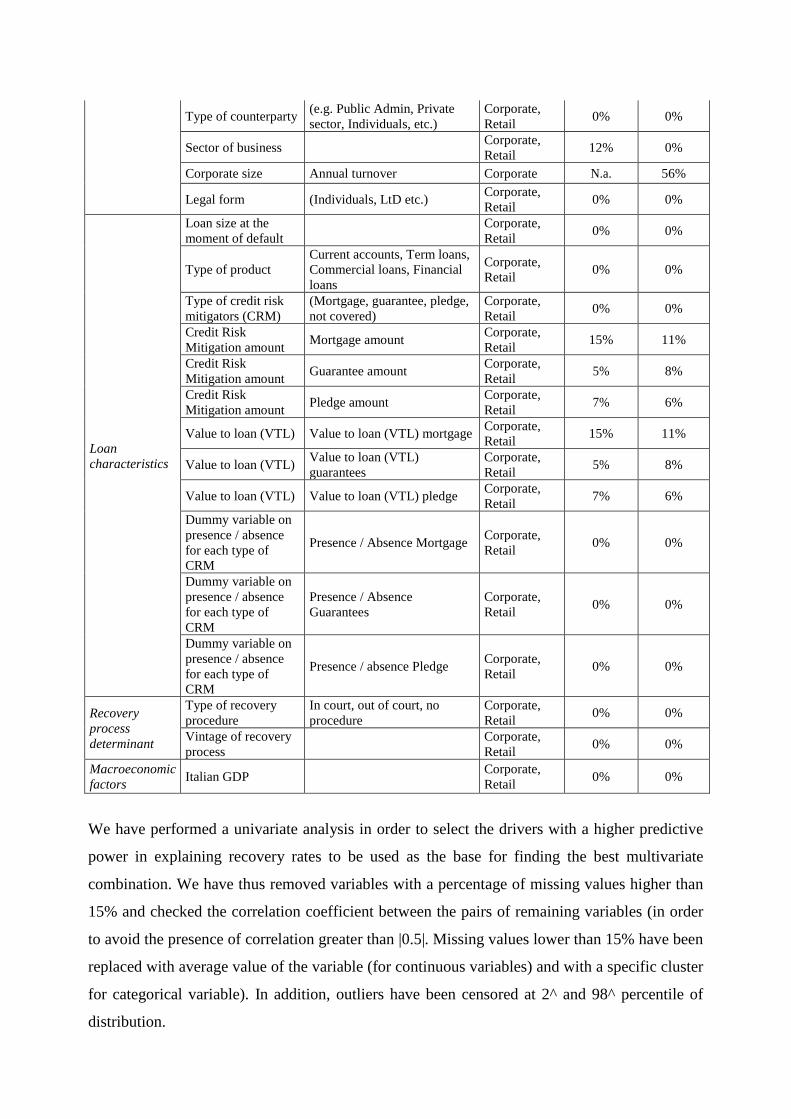
Type of counterparty (e.g. Public Admin, Private

sector, Individuals, etc.)

Corporate,

Retail 0% 0%

Sector of business Corporate,

Retail 12% 0%

Corporate size Annual turnover Corporate N.a. 56%

Legal form (Individuals, LtD etc.) Corporate,

Retail 0% 0%

Loan

characteristics

Loan size at the

moment of default

Corporate,

Retail 0% 0%

Type of product

Current accounts, Term loans,

Commercial loans, Financial

loans

Corporate,

Retail 0% 0%

Type of credit risk

mitigators (CRM)

(Mortgage, guarantee, pledge,

not covered)

Corporate,

Retail 0% 0%

Credit Risk

Mitigation amount Mortgage amount

Corporate,

Retail 15% 11%

Credit Risk

Mitigation amount Guarantee amount

Corporate,

Retail 5% 8%

Credit Risk

Mitigation amount Pledge amount

Corporate,

Retail 7% 6%

Value to loan (VTL) Value to loan (VTL) mortgage Corporate,

Retail 15% 11%

Value to loan (VTL) Value to loan (VTL)

guarantees

Corporate,

Retail 5% 8%

Value to loan (VTL) Value to loan (VTL) pledge Corporate,

Retail 7% 6%

Dummy variable on

presence / absence

for each type of

CRM

Presence / Absence Mortgage Corporate,

Retail 0% 0%

Dummy variable on

presence / absence

for each type of

CRM

Presence / Absence

Guarantees

Corporate,

Retail 0% 0%

Dummy variable on

presence / absence

for each type of

CRM

Presence / absence Pledge Corporate,

Retail 0% 0%

Recovery

process

determinant

Type of recovery

procedure

In court, out of court, no

procedure

Corporate,

Retail 0% 0%

Vintage of recovery

process

Corporate,

Retail 0% 0%

Macroeconomic

factors Italian GDP

Corporate,

Retail 0% 0%

We have performed a univariate analysis in order to select the drivers with a higher predictive

power in explaining recovery rates to be used as the base for finding the best multivariate

combination. We have thus removed variables with a percentage of missing values higher than

15% and checked the correlation coefficient between the pairs of remaining variables (in order

to avoid the presence of correlation greater than |0.5|. Missing values lower than 15% have been

replaced with average value of the variable (for continuous variables) and with a specific cluster

for categorical variable). In addition, outliers have been censored at 2^ and 98^ percentile of

distribution.

3.3.1 Multivariate econometric model specification

Starting from results of other research studies, we have applied on our data an Ordinary Least

Square Linear (OLS) regression in order to identify the best combination of variables in predicting

recovery rates.

The linear regression model is specified as:

[4]

[5]

Here the list of final variables selected for the multivariate analysis:

Table 4 – Variables selected for multivariate model

Information

group Factors Factors description Segment of application

Selected on

Retail

Selected on

Corporate

Borrower

characteristics

Geographical area

North – West,

North, East, Center,

South, Islands

Corporate, Retail YES YES

Industry Corporate, Retail NO YES

Type of

counterparty

(e.g. Public Admin,

Private sector,

Individuals, etc.)

Corporate, Retail YES YES

Sector of business Corporate, Retail YES YES

Corporate size Annual turnover Corporate N.a. NO

Legal form (Individuals, LtD

etc.) Corporate, Retail YES YES

Loan

characteristics

Loan size at the

moment of default Corporate, Retail YES YES

Type of product

Current accounts,

Term loans,

Commercial loans,

Financial loans

Corporate, Retail YES YES

Type of credit risk

mitigators (CRM)

(Mortgage,

guarantee, pledge,

not covered)

Corporate, Retail YES YES

Credit Risk

Mitigation amount Mortgage amount Corporate, Retail YES YES

Credit Risk

Mitigation amount Guarantee amount Corporate, Retail YES YES

Credit Risk

Mitigation amount Pledge amount Corporate, Retail YES YES

Value to loan

(VTL)

Value to loan

(VTL) mortgage Corporate, Retail YES YES

Value to loan

(VTL)

Value to loan

(VTL) guarantees Corporate, Retail YES YES

Value to loan

(VTL)

Value to loan

(VTL) pledge Corporate, Retail YES YES

Dummy variable on

presence / absence

for each type of

CRM

Presence / Absence

Mortgage Corporate, Retail YES YES

Dummy variable on

presence / absence

for each type of

CRM

Presence / Absence

Guarantees Corporate, Retail YES YES

Dummy variable on

presence / absence

for each type of

CRM

Presence / absence

Pledge Corporate, Retail YES YES

Recovery

process

determinant

Type of recovery

procedure

In court, out of

court, no procedure Corporate, Retail YES YES

Vintage of recovery

process Corporate, Retail YES YES

Macroeconomic

factors Italian GDP Corporate, Retail YES YES

3.4 Sample description

The framework proposed has been applied on a sample of 26,000 charge-offs with a closed

recovery process between 30/09/2002 and 31/12/2012 so composed:

Table 5 – Sample description for customer segment

Customer segment # OBS % obs Average LGD

Retail customers 15,000 57,80% 44,00%

Small –medium size Corporate (Retail) 3,500 13,50% 47,00%

Medium – Large size Corporate 7,500 28,70% 50,00%

Table 6 – Sample description for sector of activity

Sector of activity # obs. % obs.

Industry 18.341 70,54%

Commerce 3.000 11,54%

Building & Construction 889 3,42%

Services 2.500 9,62%

Transportation 383 1,47%

Agricolture 887 3,41%

Table 7 – Sample description for product type

Product type # obs. % obs.

Check accounts 16.453 63,28%

Term loans 7.138 27,45%

Advance invoices 1.611 6,20%

Other loans 677 2,60%

Credit commitments 121 0,47%

3.5 Empirical results

The spread estimated adopting CAPM framework assumes values in a range [0,8% - 1,67%] as

shown in the table below:

Table 8 – Final spread estimated with CAPM framework

Segment σi ρi,m σm MRP beta SPREAD

Corporate 0,1747 0,0827 0,2425 0,056 0,2072 1,160%

Large Corporate 0,1747 0,1431 0,2425 0,056 0,2725 1,526%

Other Retail 0,2233 0,0750 0,2425 0,056 0,2522 1,412%

Retail Mortgages 0,1866 0,1500 0,2425 0,056 0,2979 1,668%

Retail Rotative 0,1772 0,0400 0,2425 0,056 0,1461 0,818%

Other 0,1772 0,0400 0,1461 0,818%

Table 9 – Final discount rate (comparison among different approaches)

Discount rate calculation Avg.rate Std.Dev.Rate Avg. LGD Std.Dev.LGD

Only Risk-free 2,347% 1,80% 48,74% 105,26%

Risk free + Spread (CAPM) 3,562% 1,82% 49,83% 103,92%

Cost of funding 2,975% 2,33% 49,81% 106,80%

The adopted approach ensures conservatism to LGD estimates and decrease the overall volatility

of recovery distribution, mainly described in the next Table:

Table 10 – LGD Distribution

Metrics Economic LGD

Mean 49,83%

# of Missing values 0

# obs. 26.000

Min -487,28%

p1 0,4580%

p5 2,78%

p10 5,73%

p25 20,44%

p50 40,81%

p75 90,26%

p90 100,00%

p95 100,23%

p99 106,49%

Max 234,44%

Before estimating the model this distribution has been subject to censoring in [0%, 100%].

We have finally identified that the best determinants of recoveries are related to geographical

area, exposure at default, type of product and different types of credit risk mitigators, has shown

below:

Table 11 –Final model description

Variables Grouping Coefficient p-value Variable weight

Intercept 0,1001 <,0001

Macro-geographical area

Center 0,2145

<,0001

13,87%

North East 0,1113

Sud & Island 0,0788

North West 0

Exposure at Default EAD 0,1567 <,0001 10,13%

Portfoglio segmentation

Medium – Large Corporate 0,5944 0,0033 38,4% Small Business (Retail) 0,377 0,0022

Individuals (Retail) 0 <,0001

Type of product Mortgages 0,1876

<,0001

12,13% Other products 0

Presence of personal guarantess Absence 0,1134

<,0001

7,33% Presence 0

Presence of mortgages

Absence

0,1609

<,0001

10,40%

Presence 0

Type of recovery process

Out of court 0,1189 <,0001

7,69% In court 0,0533

No information 0

The backtesting performed on the development sample has shown an Accuracy Ratio of final

model of 57% and an AUROC (Area Under the ROC Curve) of 75%. The model has an

Adjusted R-square of 31%.

4. Conclusions

This paper has presented a case study of LGD in which, according to the requirements of

Basel2, the model has been developed on 10 years of historical real data of Corporate and

Retail portfolio of a panel of commercial banks under ECB supervision. Giving a particular

stress on the economic component of the model, the presented model highlights the

determinant role of mitigators as recovery drivers, but also the geographical localization of

loans, the type of product and the exposure at default. Our paper contributes to the strand of

the literature studying the determinants of recovery rates on real portfolio of Corporate and

Retail loans under the new Credit Risk Regulatory environment. The paper also provides a

comparative analysis among different ways of defining discount rate and estimating

recoveries, chosing CAPM for discounting cash flows and a linear regression approach for

forecasting losses. Finally, this paper is really important since the existence of very few

analyses on recovery rates of bank loans focused on continental Europe, having found that

the most part of research on recoveries are focused on Bond US Market. A further

development of this research could be the comparison of different approaches for

multivariate model definition, starting from the main findings from literature review.

DECLARATION OF INTEREST: There is no conflict of interests: all the contents of this paper are under the

authors responsibility.

References

1. Altman, E., Brady, E., Resti, A. and Sironi, A. (2005). The Link between Default and

Recovery Rates: Theory, Empirical Evidence, and Implications. The Journal of Business 78

(6), 2203-2228

2. Altman, E., (2008). Default Recovery Rates and LGD in Credit Risk Modeling and Practice:

an updated review of the literature and empirical evidence. In Advances in Credit Risk

Modelling and Corporate Bankruptcy Prediction Book (Stewart Jones ed.), 175-206

3. Araten, M., Jacobs, M., and Varshney, P. (2004). Measuring LGD on Commercial Loans: An

18-Year Internal Study. RMA Journal 86 (8), 28-35

4. Bastos J.A. (2010). Forecasting bank loans Loss Given Default. Journal of Banking and

Finance 34 (10), 2510-2517

5. Bellotti, T., Crook, J. (2012). Loss given default models incorporating macroeconomic

variables for credit cards. International Journal of Forecasting Vol. 28 (171-182)

6. Bonini. S. and Caivano, G. (2014). Estimating loss-given default through advanced

credibility theory. The European Journal of Finance 10.1080/1351847X.2013.870918

7. Bonini. S. and Caivano, G. (2013). Survival analysis approach in Basel2 Credit Risk

Management: modelling Danger Rates in Loss Given Default parameter. Journal of Credit

Risk 9 (1)

8. Carty L.V., Gates D. and Gupton G.M. (2000). Bank Loss Given Default. Moody's Investors

Service, Global Credit Research

9. Chalupa, R., and Kopecsni, J. (2009). Modeling Bank Loan LGD of Corporate and SME

Segments: A Case Study. Czech Journal of Economics and Finance 59 (4)

10. Dermine, J., and Neto de Carvalho, C. (2005). Bank loan losses-given-default: A case study.

The Journal of Banking and Finance 30 (4), 1219-1243

11. European Banking Authority: Guidelines on PD estimation, LGD estimation and the

treatment of defaulted exposures. Consultation Paper (2016)

12. European Central Bank: Guide for the Targeted Review of Internal Models. ECB Publication

(2017)

13. European Union: Regulation (EU) No 575/2013 of the European Parliament and of the

Council of 26 June 2013 on prudential requirements for credit institutions and investment

firms and amending Regulation (EU) No 648/2012. Official Journal of the European Union

(2013)

14. Fernandez, P., Aguirreamalloa, J. and Corres, L. (2012). “Market Risk Premium used in 82

countries in 2012: a survey with 7,192 answers”. IESE Business School publication

15. Frontczazk, R., Rostek, S. (2015). Modeling loss given default with stochastic collateral.

Economic Modelling 44, 162 - 170

16. Gupton, G. M., and Stein, R. M. (2005). LossCalc: Model for Predicting Loss Given Default

(LGD). Moody’s KMV publication

17. Gürtler, M. and Hibbeln, M (2013). Improvements in Loss Given Default Forecasts for Bank

Loans. Journal of Banking and Finance 37 (7), 2354–2366

18. Grunet, J., and Weber,M. (2009). Recovery rates of commercial lending: empirical evidence

for German companies. Journal of Banking and Finance 33, 505–513

19. Hwang, R.C. and Chu C.C. (2017). A logistic regression point of view toward loss given

default distribution estimation. Journal of Quantitative Finance

20. Jokivoulle E. and Peura S. (2003). Incorporating Collateral Value Uncertainty in Loss Given

Default Estimates and Loan-to-value Ratios. European Financial Management 9, 299 - 314

21. Khieu H.D., Mullineaux D.M. and Yi H. (2012). The determinants of bank loan recovery

rates. Journal of Banking & Finance 36 (4), 923-933

22. Leow M. and Mues C. (2012). Predicting loss given default (LGD) for residential mortgage

loans: A two-stage model and empirical evidence for UK bank data. International Journal of

Forecasting 28 (1), 183–195

23. Malkani R. (2012). A realistic approach for estimating and modeling loss given default. The

Journal of Risk Model Validation 6 (2), 103 - 116

24. Maclahan, I. (2004). Choosing the Discount Factor for Estimating Economic LGD, in

Recovery Risk: The Next Challenge in Credit Risk Management. by Altman, E., Resti, A. &

Sironi A.

25. Matuszyk A., and Mues C., Thomas L.C. (2010). Modeling LGD for unsecured personal

loans: Decision tree approach. Journal of the Operational Research Society 3 (61), 393-398

26. Miller P., Tows E. (2017). Loss given default adjusted workout processes for leases. Journal

of Banking and Finance

27. Morrison, J.S. (2004). Preparing for Basel II Common Problems, Practical Solutions. RMA

Journal

28. Qi, M., Zhao, X. (2011). Comparison of modeling methods for loss given default, Journal of

Banking and Finance Vol. 35 (2842-2855)

29. Schuermann, T. (2004), What Do We Know About Loss Given Default?, Working paper on

Wharton Financial Institutions Center

30. Yang H.B. (2012). Modeling exposure at default and loss given default: empirical

approaches and technical implementation. Journal of Credit Risk 8 (2), 81 - 102

31. Yashir, O., and Yashir, Y. (2012). Loss given default modeling: a comparative analysis.

Journal of Risk Model Validation 7 (1), 25–59

32. Witzany, J., Rychnovsky´, M., and Charamza, P. (2010). Survival Analysis in LGD

Modeling. IES Working Paper 2/2010