ECIV 301

Programming & Graphics

Numerical Methods for Engineers

REVIEW II

Topics

• Introduction to Matrix Algebra• Gauss Elimination• LU Decomposition• Matrix Inversion• Iterative Methods

• Function Interpolation & Approximation• Newton Polynomials• Lagrange Polynomials

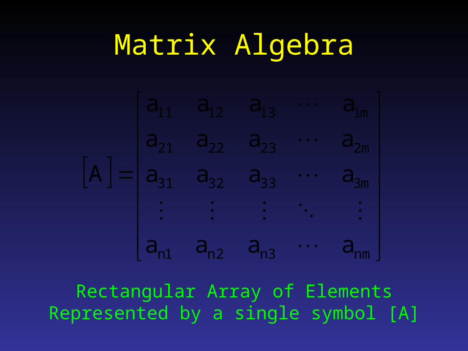
Matrix Algebra

nm3n2n1n

m3333231

m2232221

m1131211

aaaa

aaaa

aaaa

aaaa

A

Rectangular Array of Elements Represented by a single symbol [A]

Matrix Algebra

nm3n2n1n

m3333231

m2232221

m1131211

aaaa

aaaa

aaaa

aaaa

A

Row 1

Row 3

Column 2 Column m

n x m Matrix

nm3n2n1n

m3333231

m2232221

m1131211

aaaa

aaaa

aaaa

aaaa

A

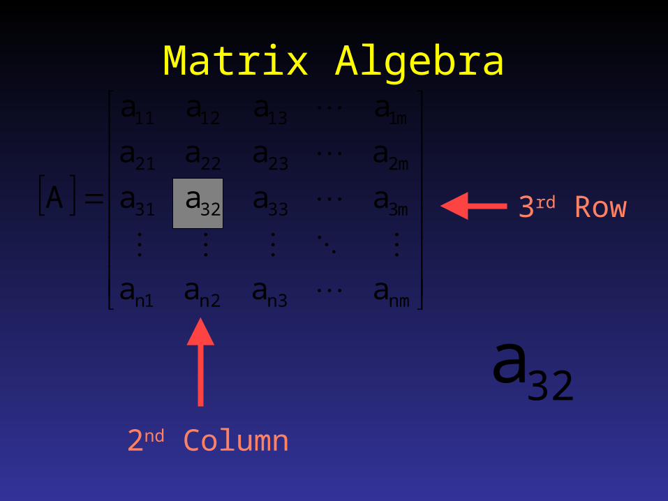
Matrix Algebra

32a

3rd Row

2nd Column

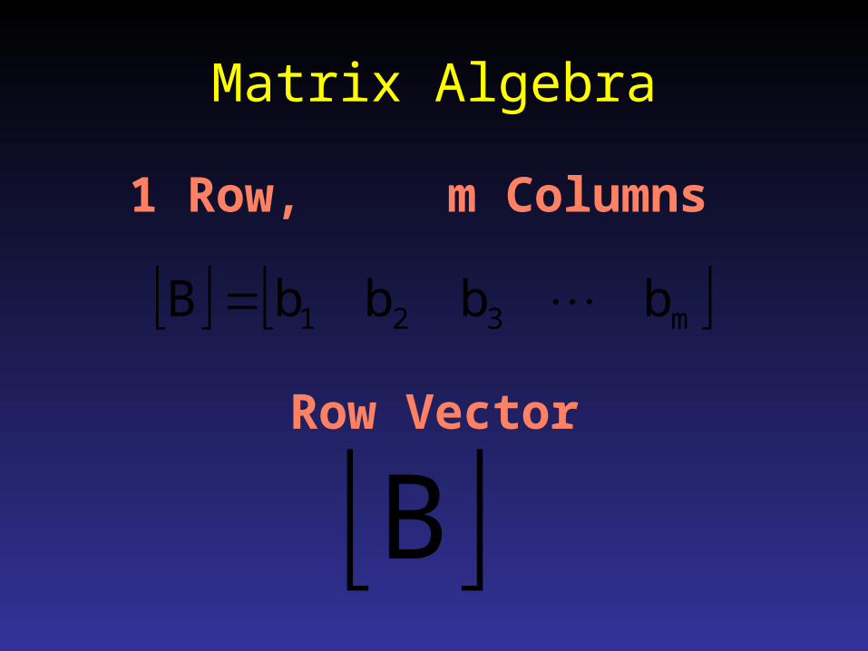
Matrix Algebra

m321 bbbbB

1 Row, m Columns

Row Vector

B

Matrix Algebra

n

3

2

1

c

c

c

c

C

n Rows, 1 Column

Column Vector

C

Matrix Algebra

5554535251

4544434241

3534333231

2524232221

1514131211

aaaaa

aaaaa

aaaaa

aaaaa

aaaaa

A

If n = m Square Matrix

e.g. n=m=5e.g. n=m=5Main Diagonal

Matrix Algebra

9264

2732

6381

4215

A

Special Types of Square Matrices

Symmetric: aSymmetric: aijij = a = ajiji

Matrix Algebra

9000

0700

0080

0005

A

Diagonal: aDiagonal: aijij = 0, i = 0, ijj

Special Types of Square Matrices

Matrix Algebra

1000

0100

0010

0001

I

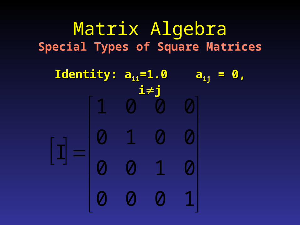
Identity: aIdentity: aiiii=1.0 a=1.0 aijij = 0, i = 0, ijj

Special Types of Square Matrices

nm

m333

m22322

m1131211

a000

aa00

aaa0

aaaa

A

Matrix Algebra

Upper TriangularUpper Triangular

Special Types of Square Matrices

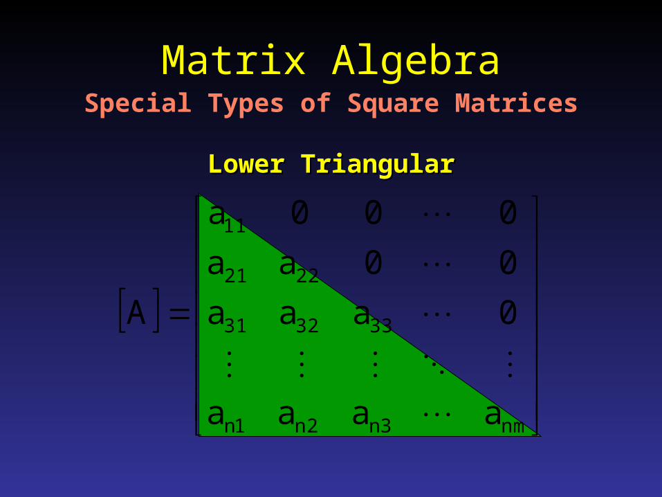
nm3n2n1n

333231

2221

11

aaaa

0aaa

00aa

000a

A

Matrix Algebra

Lower TriangularLower Triangular

Special Types of Square Matrices

nm

3332

232221

1211

a000

0aa0

0aaa

00aa

A

Matrix Algebra

BandedBanded

Special Types of Square Matrices

Matrix Operating Rules - Equality

nm3n2n1n

m3333231

m2232221

m1131211

aaaa

aaaa

aaaa

aaaa

A

pq3p2p1p

q3333231

q2232221

q1131211

bbbb

bbab

bbbb

bbbb

B

[A]mxn=[B]pxq

n=p m=q aij=bij

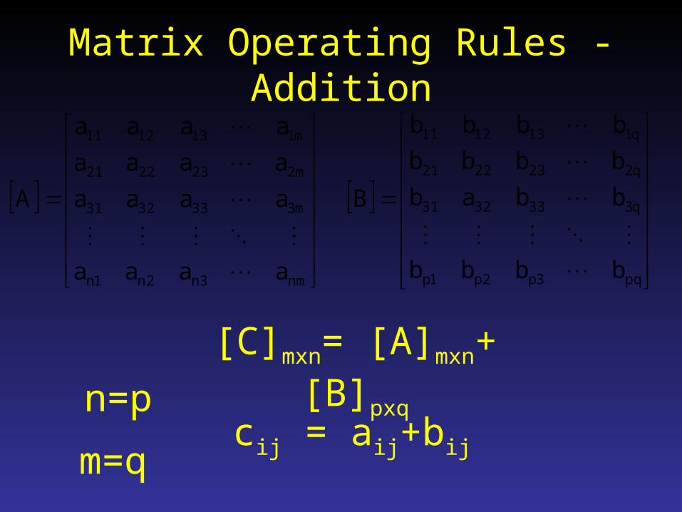
Matrix Operating Rules - Addition

nm3n2n1n

m3333231

m2232221

m1131211

aaaa

aaaa

aaaa

aaaa

A

pq3p2p1p

q3333231

q2232221

q1131211

bbbb

bbab

bbbb

bbbb

B

[C]mxn= [A]mxn+[B]pxq

n=p

m=qcij = aij+bij

Matrix Operating Rules - Addition

Properties

[A]+[B] = [B]+[A]

[A]+([B]+[C]) = ([A]+[B])+[C]

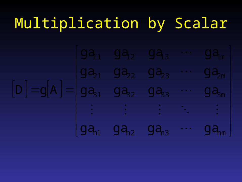
Multiplication by Scalar

nm3n2n1n

m3333231

m2232221

m1131211

gagagaga

gagagaga

gagagaga

gagagaga

AgD

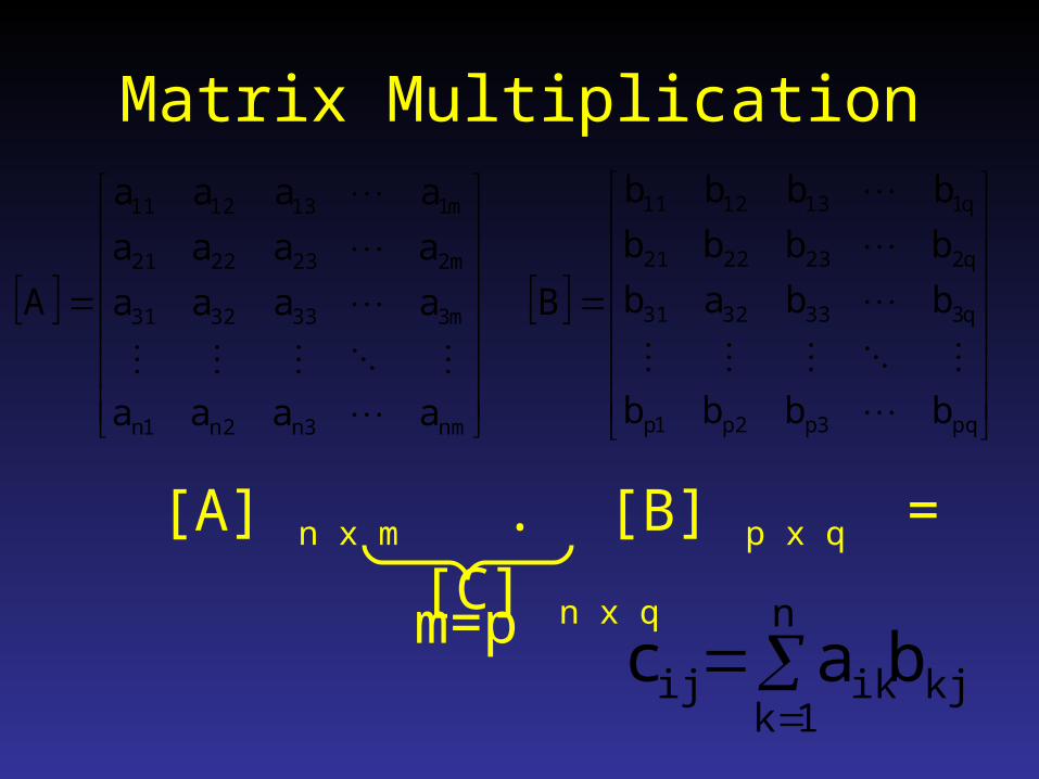
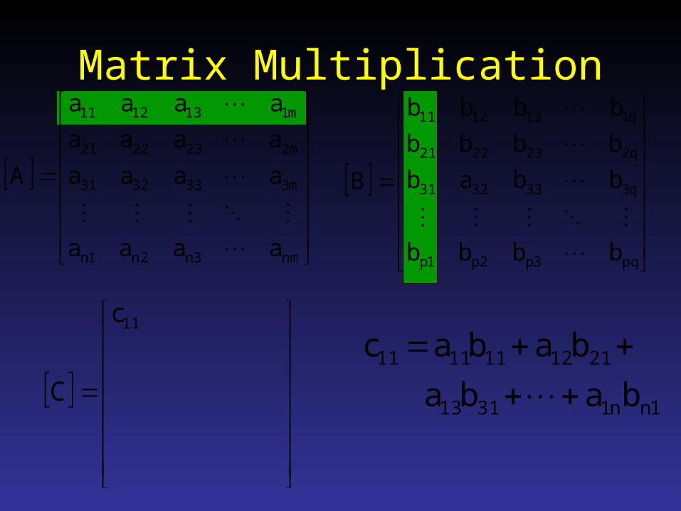
Matrix Multiplication

nm3n2n1n

m3333231

m2232221

m1131211

aaaa

aaaa

aaaa

aaaa

A

pq3p2p1p

q3333231

q2232221

q1131211

bbbb

bbab

bbbb

bbbb

B

[A] n x m . [B] p x q = [C] n x q

m=p

n

1kkjikij bac

Matrix Multiplication

nm3n2n1n

m3333231

m2232221

m1131211

aaaa

aaaa

aaaa

aaaa

A

pq3p2p1p

q3333231

q2232221

q1131211

bbbb

bbab

bbbb

bbbb

B

1nn13113

2112111111

baba

babac

11c

C

nm3n2n1n

m3333231

m2232221

m1131211

aaaa

aaaa

aaaa

aaaa

A

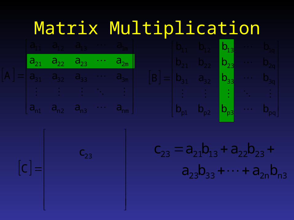
Matrix Multiplication

pq3p2p1p

q3333231

q2232221

q1131211

bbbb

bbab

bbbb

bbbb

B

3nn23323

2322132123

baba

babac

23c

C

Matrix Multiplication - Properties

Associative: [A]([B][C]) = ([A][B])[C]

If dimensions suitable

Distributive: [A]([B]+[C]) = [A][B]+[A] [C]

Attention: [A][B] [B][A]

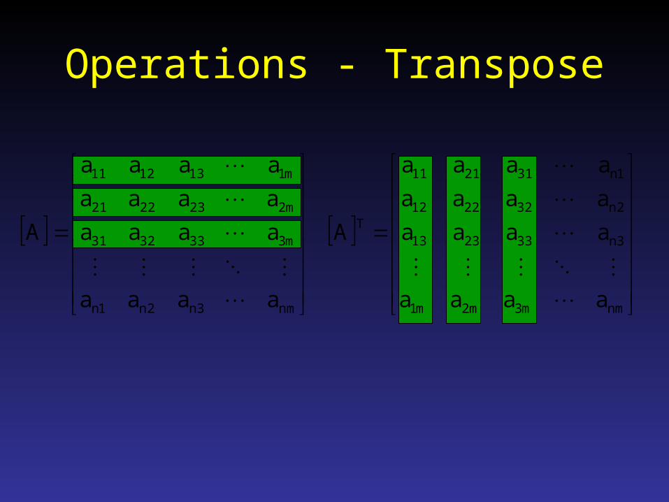
nmm3m2m1

3n332313

2n322212

1n312111

T

aaaa

aaaa

aaaa

aaaa

A

nm3n2n1n

m3333231

m2232221

m1131211

aaaa

aaaa

aaaa

aaaa

A

Operations - Transpose

Operations - Inverse

[A] [A]-1

[A] [A]-1=[I]

If [A]-1 does not exist[A] is singular

Operations - Trace

5554535251

4544434241

3534333231

2524232221

1514131211

aaaaa

aaaaa

aaaaa

aaaaa

aaaaa

A

Square Matrix

tr[A] = tr[A] = aaiiii

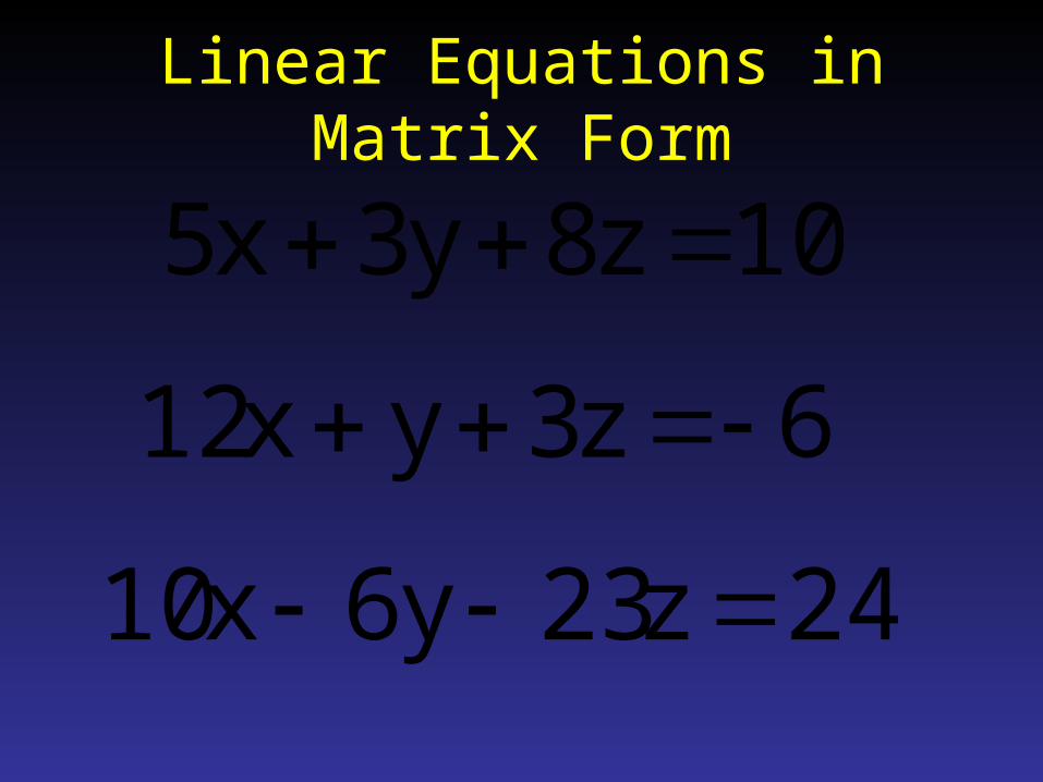
Linear Equations in Matrix Form

10z8y3x5

6z3yx12

24z23y6x10

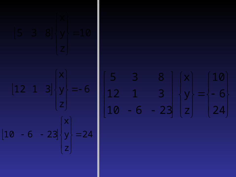
23610

3112

835

z

y

x

24

6

10 6

z

y

x

3112

24

z

y

x

23610

10

z

y

x

835

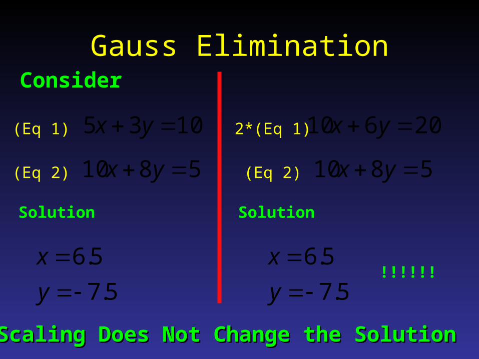
Gauss EliminationConsider

1035 yx(Eq 1)

5810 yx(Eq 2)

Solution

5.7

5.6

y

x

20610 yx2*(Eq 1)

5810 yx(Eq 2)

Solution

5.7

5.6

y

x!!!!!!

Scaling Does Not Change the SolutionScaling Does Not Change the Solution

Gauss EliminationConsider

20610 yx(Eq 1)

152 y(Eq 2)-(Eq 1)

Solution

5.7

5.6

y

x!!!!!!

20610 yx(Eq 1)

5810 yx(Eq 2)

Solution

5.7

5.6

y

x

Operations Do Not Change the SolutionOperations Do Not Change the Solution

Gauss Elimination

10835 zyx

2423610 zyx

6312 zyx

Example

Forward Elimination

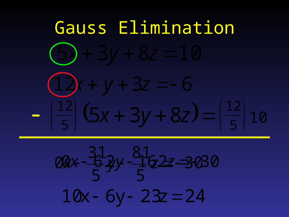
Gauss Elimination

10835 zyx

24z23y6x10

zyx 835

5

1210

5

12

6312 zyx

-

305

81

5

310 zyx 302.162.60 zyx

Gauss Elimination

10835 zyx

24z23y6x10

6312 zyx 302.162.60 zyx

Substitute 2nd eq with new

Gauss Elimination

10835 zyx

24z23y6x10

302.162.60 zyx

zyx 835

5

1010

5

10-

439120 zyx

Gauss Elimination

10835 zyx

24z23y6x10

302.162.60 zyx

Substitute 3rd eq with new

439120 zyx

Gauss Elimination

10835 zyx

302.162.60 zyx

439120 zyx

zy 2.162.6

2.6

12 30

2.6

12-

064.62645.700 zyx

Gauss Elimination

10835 zyx

30970 zyx

Substitute 3rd eq with new

439120 zyx 064.62645.700 zyx

Gauss Elimination

Forward Elimination

064.62

30

10

645.700

2.162.60

835

z

y

x

Gauss Elimination

Back Substitution

118.8645.7/064.62 z

0502.26

2.6

118.82.1630

y

6413.0

5

118.880502.26310

x

064.62

30

10

645.700

2.162.60

835

z

y

x

Gauss Elimination – Potential Problem

10830 zyx

2423610 zyx

6312 zyx

Pivoting

6312 zyx

10830 zyx

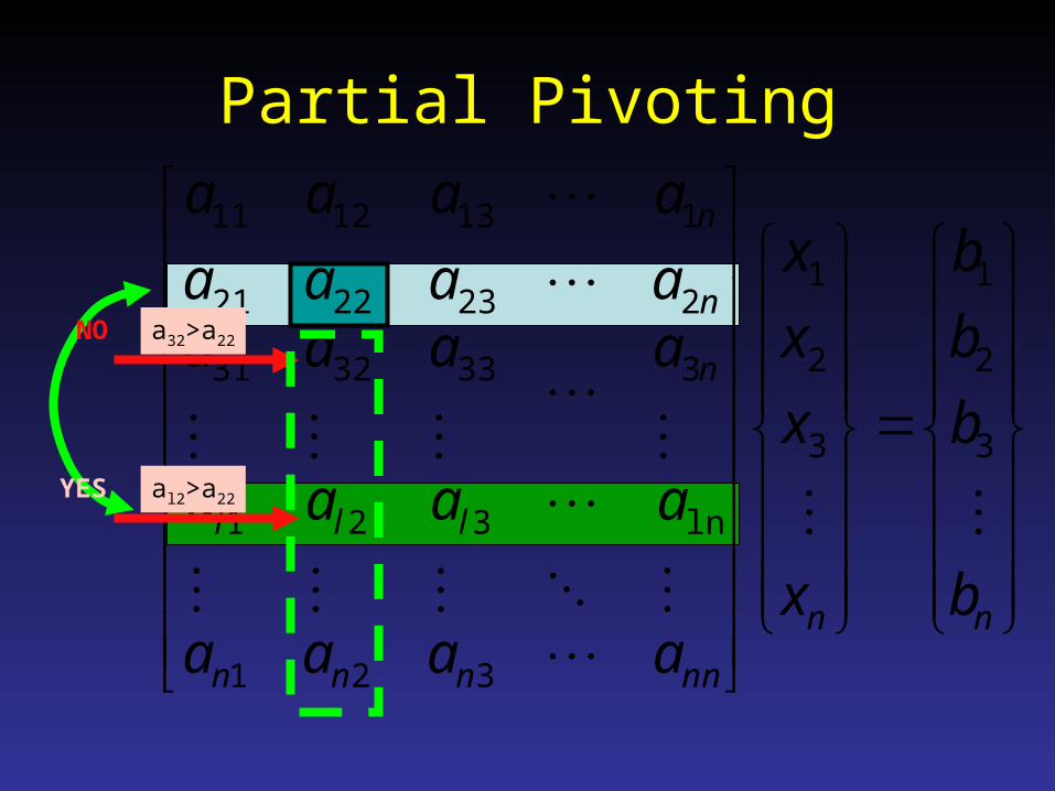
Partial Pivoting

nn

nnnnn

lll

n

n

n

b

b

b

b

x

x

x

x

aaaa

aaaa

aaaaaaaa

aaaa

3

2

1

3

2

1

321

ln321

3333231

2232221

1131211

a32>a22

al2>a22

NO

YES

Partial Pivoting

nn

nnnnn

n

n

lll

n

b

b

b

b

x

x

x

x

aaaa

aaaa

aaaaaaaa

aaaa

3

2

1

3

2

1

321

2232221

3333231

ln321

1131211

Full Pivoting

• In addition to row swaping

• Search columns for max elements

• Swap Columns

• Change the order of xi

• Most cases not necessary

LU Decomposition

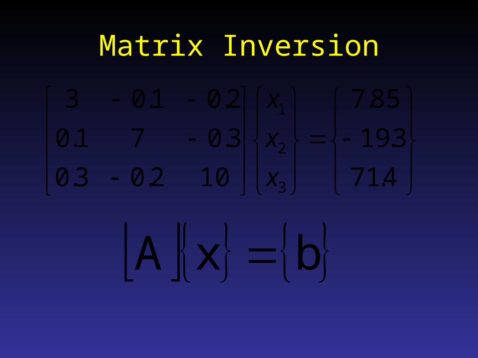
4.71

3.19

85.7

102.03.0

3.071.0

2.01.03

3

2

1

x

x

x

LU DecompositionPIVOTS

Column 1PIVOTS

Column 2

03333.0

1.0 02713.0

LU Decomposition

As many as, and in the location of, zeros

UpperTriangular

MatrixU

01200.1000

29333.000333.70

2.01.03

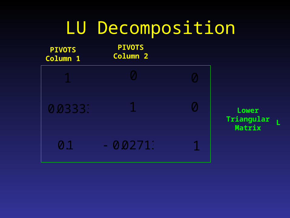
LU DecompositionPIVOTS

Column 1

PIVOTSColumn 2

LowerTriangular

Matrix

1

1

1

0

0

0

L

03333.0

1.0 02713.0

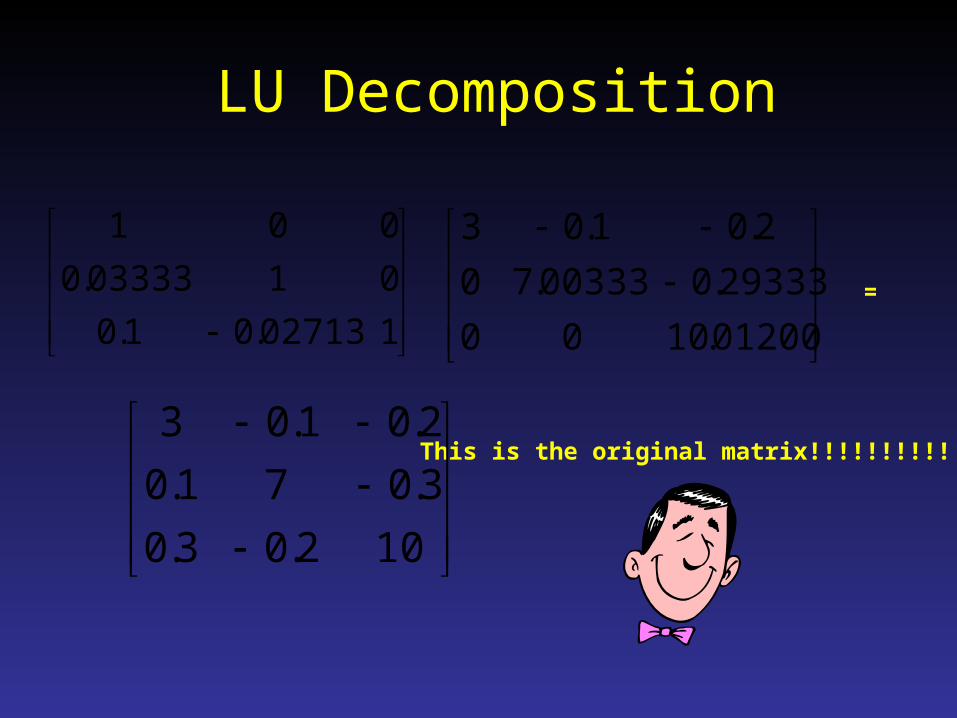
LU Decomposition

102713.01.0

0103333.0

001

=

This is the original matrix!!!!!!!!!!

01200.1000

29333.000333.70

2.01.03

102.03.0

3.071.0

2.01.03

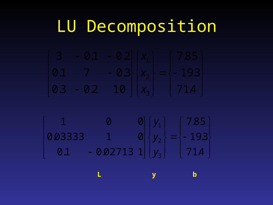
LU Decomposition

4.71

3.19

85.7

102713.01.0

0103333.0

001

3

2

1

y

y

y

4.71

3.19

85.7

102.03.0

3.071.0

2.01.03

3

2

1

x

x

x

L y b

LU Decomposition

4.71

3.19

85.7

102713.01.0

0103333.0

001

3

2

1

y

y

y

L y b

85.71 y

5617.190333.03.19 12 yy

0843.70)02713.0(1.04.71 213 yyy

LU Decomposition85.71 y

5617.190333.03.19 12 yy

0843.70)02713.0(1.04.71 213 yyy

0843.70

5617.19

85.7

01200.1000

29333.000333.70

2.01.03

LU Decomposition

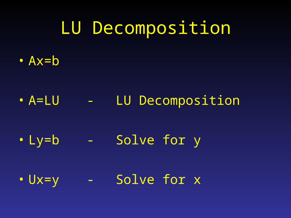
• Ax=b

• A=LU - LU Decomposition

• Ly=b- Solve for y

• Ux=y - Solve for x

Matrix Inversion

4.71

3.19

85.7

102.03.0

3.071.0

2.01.03

3

2

1

x

x

x

bxA

Matrix Inversion

[A] [A]-1

[A] [A]-1=[I]

If [A]-1 does not exist[A] is singular

Matrix Inversion

b xA bxA 1A 1A

I

Matrix Inversion

bAx 1

Solution

Matrix Inversion

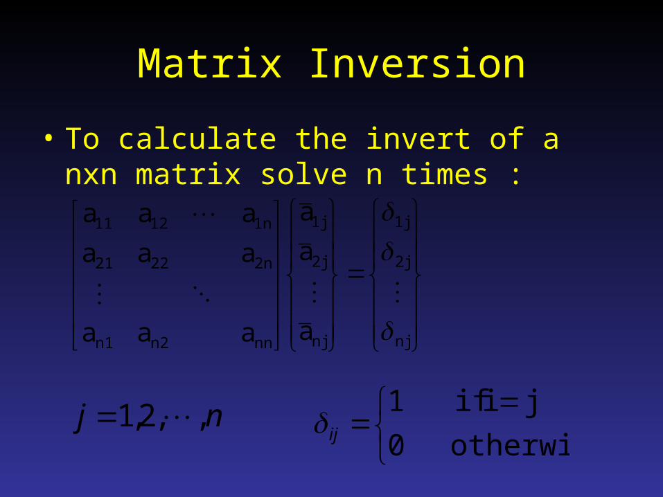
• To calculate the invert of a nxn matrix solve n times :

nj

2j

1j

nj

2j

1j

nnn2n1

2n2221

1n1211

a

a

a

aaa

aaa

aaa

nj ,,2,1

otherwise

ji if

0

1ij

Iterative Methods

Recall Techniques for Root finding of Single Equations

Initial Guess

New Estimate

Error Calculation

Repeat until Convergence

Gauss Seidel

3

2

1

3

2

1

333231

232221

131211

b

b

b

x

x

x

aaa

aaa

aaa

11

31321211 a

xaxabx

22

32312122 a

xaxabx

33

23213133 a

xaxabx

Gauss Seidel

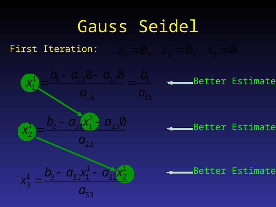
11

1

11

1312111

00

a

b

a

aabx

22

23112121

2

0

a

axabx

33

1232

113131

3 a

xaxabx

First Iteration: 0,0,0 321 xxx

Better Estimate

Better Estimate

Better Estimate

Gauss Seidel

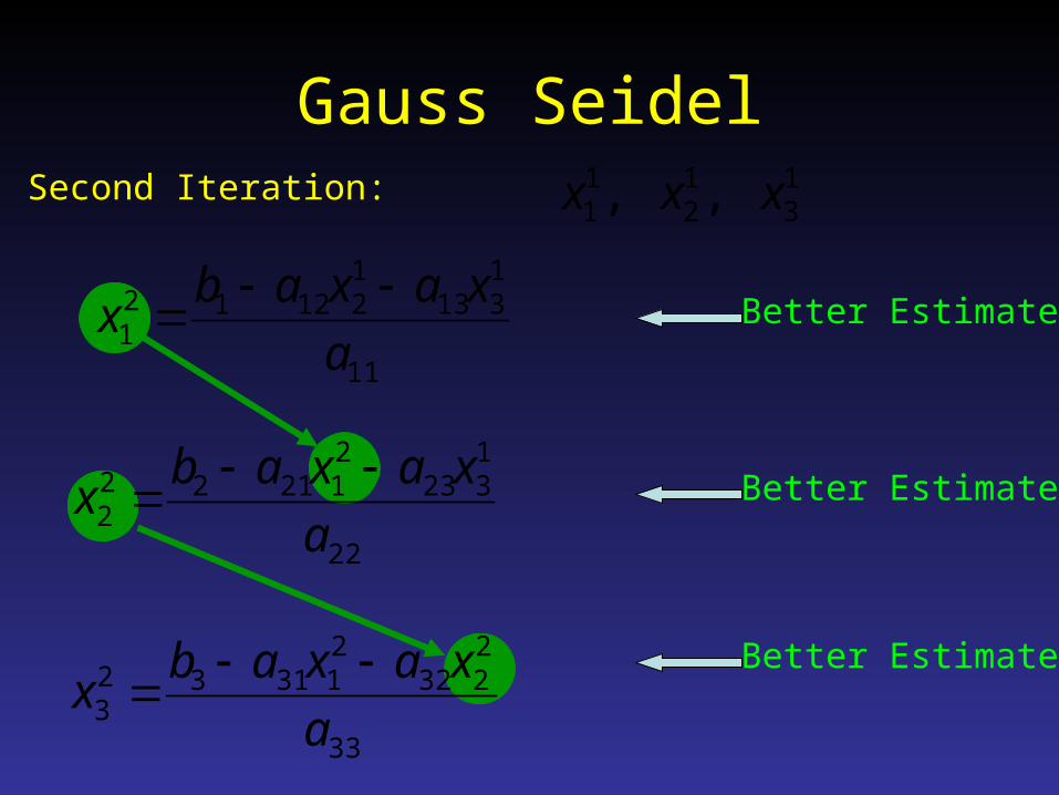
11

1313

121212

1 a

xaxabx

22

1323

212122

2 a

xaxabx

33

2232

213132

3 a

xaxabx

Second Iteration: 13

12

11 ,, xxx

Better Estimate

Better Estimate

Better Estimate

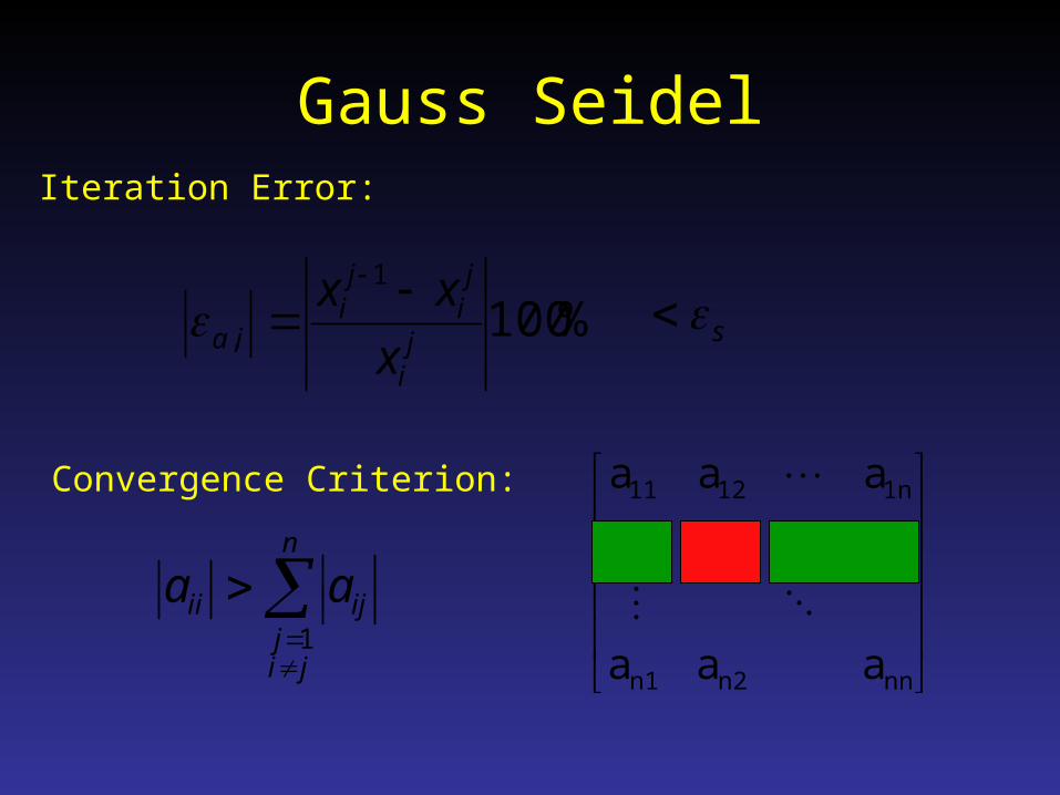
Gauss SeidelIteration Error:

%1001

, ji

ji

ji

ia x

xx

s

Convergence Criterion:

n

jij

ijii aa1

nnn2n1

2n2221

1n1211

aaa

aaa

aaa

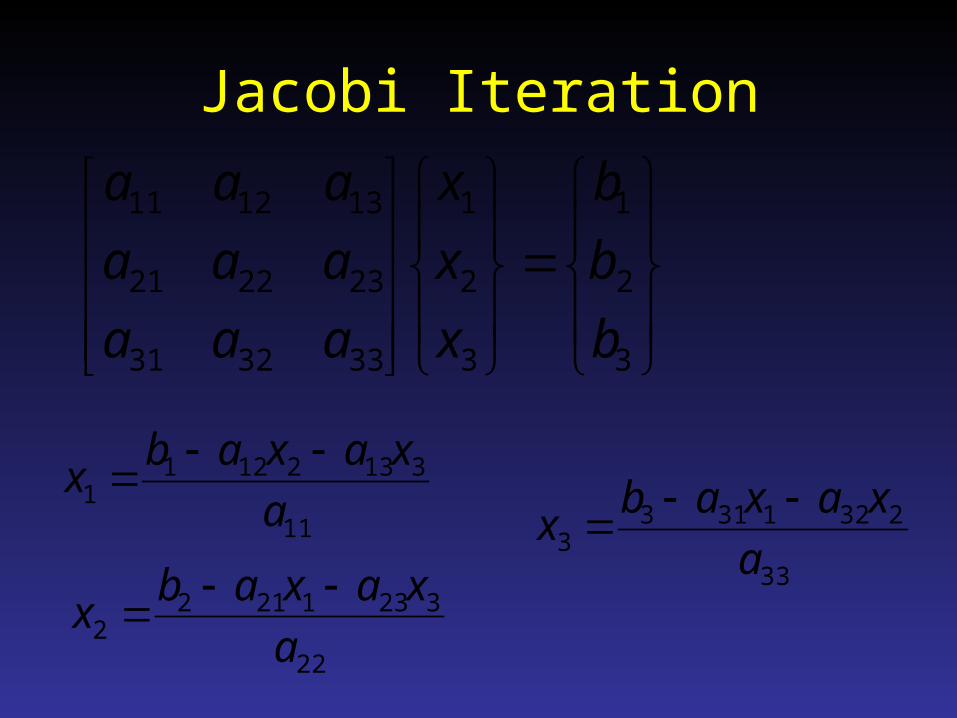
Jacobi Iteration

3

2

1

3

2

1

333231

232221

131211

b

b

b

x

x

x

aaa

aaa

aaa

11

31321211 a

xaxabx

22

32312122 a

xaxabx

33

23213133 a

xaxabx

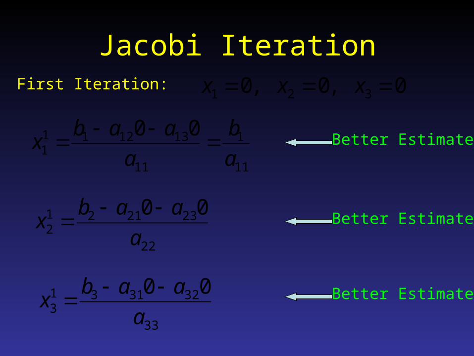
Jacobi Iteration

11

1

11

1312111

00

a

b

a

aabx

22

2321212

00

a

aabx

33

3231313

00

a

aabx

First Iteration: 0,0,0 321 xxx

Better Estimate

Better Estimate

Better Estimate

Jacobi Iteration

11

1313

121212

1 a

xaxabx

22

1323

112122

2 a

xaxabx

33

1232

113132

3 a

xaxabx

Second Iteration: 13

12

11 ,, xxx

Better Estimate

Better Estimate

Better Estimate

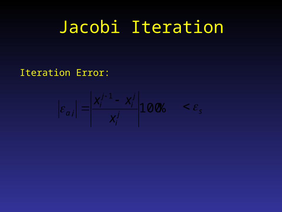
Jacobi Iteration

Iteration Error:

%1001

, ji

ji

ji

ia x

xx

s

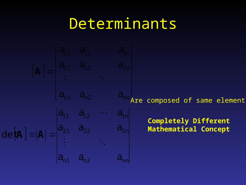
Determinants

nnn2n1

2n2221

1n1211

aaa

aaa

aaa

A

nnn2n1

2n2221

1n1211

aaa

aaa

aaa

det

AA

Are composed of same elements

Completely Different Mathematical Concept

Determinants

2221

1211

aa

aaA

Defined in a recursive form

2x2 matrix

122122112221

1211det aaaaaa

aaA

DeterminantsDefined in a recursive form

3x3 matrix

3231

222113

3331

232112

3332

232211

det

aa

aaa

aa

aaa

aa

aaa

A

333231

232221

131211

aaa

aaa

aaa

333231

232221

131211

aaa

aaa

aaa

Determinants

3332

232211 aa

aaa

3231

222113

3331

232112 aa

aaa

aa

aaa

3332

2322

aa

aaMinor a11

333231

232221

131211

aaa

aaa

aaa

Determinants

3331

2321

aa

aaMinor a12

3332

232211 aa

aaa

3331

232112 aa

aaa

3231

222113 aa

aaa

333231

232221

131211

aaa

aaa

aaa

Determinants

3231

2221

aa

aaMinor a13

3332

232211 aa

aaa

3331

232112 aa

aaa

3231

222113 aa

aaa

Singular Matrices

3

2

1

3

2

1

333231

232221

131211

b

b

b

x

x

x

aaa

aaa

aaa

If det[A]=0 solution does NOT exist

Determinants and LU Decomposition

nnaaaaD 332211det U

33

2322

131211

00

0

a

aa

aaa

)operations pivoting no (if detdet UA D

Curve Fitting

Often we are faced with the problem…

x y0.924 -0.003880.928 -0.00743

0.93283 0.005690.93875 0.00188

0.94 0.01278

-0.01

-0.005

0

0.005

0.01

0.015

0.92 0.925 0.93 0.935 0.94 0.945

what value of y corresponds to x=0.935?

-0.01

-0.005

0

0.005

0.01

0.015

0.92 0.925 0.93 0.935 0.94 0.945

Curve Fitting

Question 1: Is it possible to find a simple and convenient formula that reproduces the points exactly?

-0.01

-0.005

0

0.005

0.01

0.015

0.92 0.925 0.93 0.935 0.94 0.945

e.g. Straight Line ?

-0.01

-0.005

0

0.005

0.01

0.015

0.92 0.925 0.93 0.935 0.94 0.945

…or smooth line ?

…or some other representation?

Interpolation

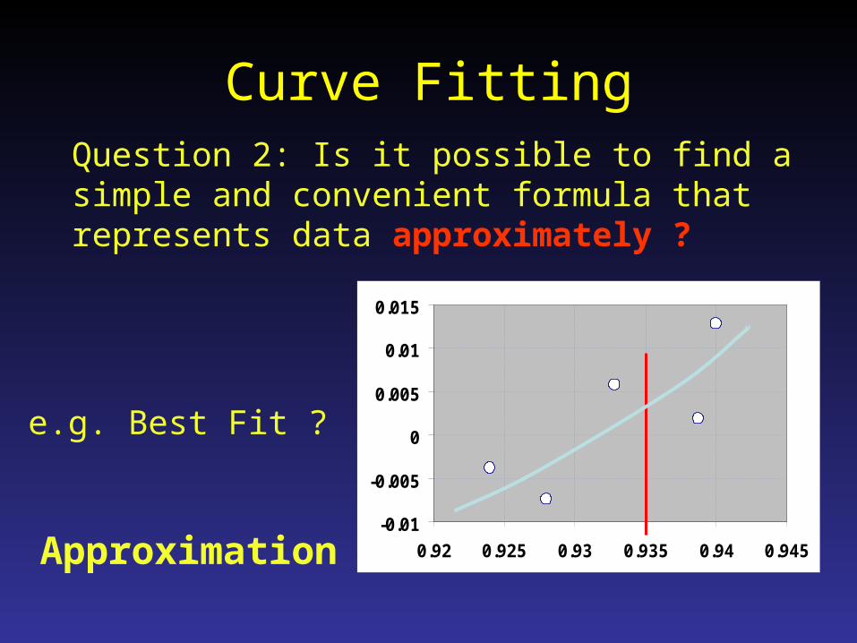
Curve FittingQuestion 2: Is it possible to find a simple and convenient formula that represents data approximately ?

-0.01

-0.005

0

0.005

0.01

0.015

0.92 0.925 0.93 0.935 0.94 0.945

e.g. Best Fit ?

Approximation

Linear Interpolation

iii

iii xx

xx

xfxfxfxf

1

11

Slope of Line

1st DIVIDED DIFFERENCEf [xi+1,xi]

First order interpolating polynomial

ii

ii

i

ii

xx

xfxf

xx

xfxf

1

11

Function Interpolation

Quadratic Interpolation

Better Accuracy if

2nd Order Polynomial -0.01

-0.005

0

0.005

0.01

0.015

0.92 0.925 0.93 0.935 0.94 0.945

x

12102 iii xxxxbxxbbxf

General Form of Newton’s Interpolating Polynomials

011 , xxfb

00 xfb

0122 ,, xxxfb

110

212

01

0

nn

n

xxxxxxb

xxxxb

xxb

b

xf

110 ,, nn xxxfb

Lagrange Interpolating Polynomials

• Reformulation of Newton’s Polynomials

• Avoid Calculation of Divided Differences

n

iiin xfxLxf

0

)()(x f(x)xo f(xo )

x1 f(x1 )

x2 f(x2 )

… …

xn f(xn)

n

ijj ji

ji xx

xxxL

0

)(

Lagrange Interpolating PolynomialCardinal Functions: Product of n-1 linear factors

ni

n

ii

i

ii

i

iii xx

xx

xx

xx

xx

xx

xx

xx

xx

xxxL

1

1

1

1

2

2

1

1

Skip xi

Property:

ji if 1

ji if 0ijji xL

Errors in Polynomial Interpolation

n321

n321

y y y yy f(x)

x x x xx

-0.01

-0.005

0

0.005

0.01

0.015

0.92 0.925 0.93 0.935 0.94 0.945

It is expected that as number of nodes increases, error decreases, HOWEVER….

n

iiin xfxLxf

11

At all interpolation nodes xi Error=0At all intermediate points

Error: f(x)-fn-1(x)

f(x)

Errors in Polynomial Interpolation

Beware of Oscillations….

For Example:Consider f(x)=(1+x2)-1 evaluated at 9 points in [-5,5]And corresponding p8(x) Lagrange Interpolating Polynomial

P8(x)f(x)

Other Methods

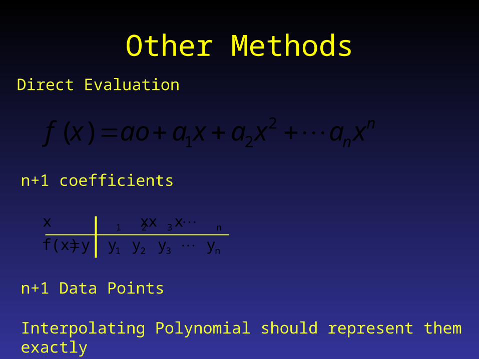
nn xaxaxaaoxf 2

21)(

Direct Evaluation

n+1 coefficients

n321

n321

y y y yy f(x)

x x x xx

n+1 Data Points

Interpolating Polynomial should represent them exactly

Other Methods

nn xaxaxaaoxf 2

21)(

Direct Evaluation

n321

n321

y y y yy f(x)

x x x xx

nn xaxaxaaoy 1

212111

nn xaxaxaaoy 2

222212

nnnnnn xaxaxaaoy 2

21

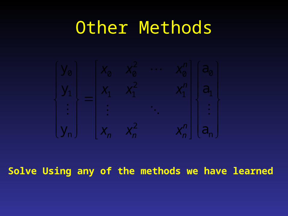
Other Methods

n

1

0

2

1211

0200

n

1

0

a

a

a

y

y

y

nnnn

n

n

xxx

xxx

xxx

Solve Using any of the methods we have learned

Other Methods

•Not the most efficient method

•Ill-conditioned matrix (nearly singular)

•If n is large highly inaccurate coefficients

•Limit to lower order polynomials

Inverse Interpolation

n321

n321

y y y yy f(x)

x x x xx

-0.01

-0.005

0

0.005

0.01

0.015

0.92 0.925 0.93 0.935 0.94 0.945

X=?X=?

Inverse Interpolation

-0.01

-0.005

0

0.005

0.01

0.015

0.92 0.925 0.93 0.935 0.94 0.945

X=?X=?

Switch x and y and then interpolate?

Not a Good Idea!

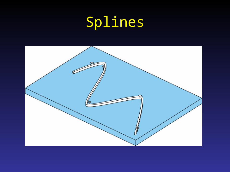
Splines

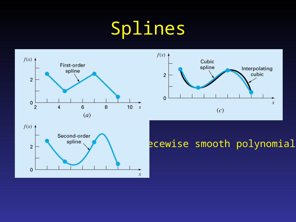
Splines

Piecewise smooth polynomials

tscoefficien n3

E.G Quadratic Splines

• Function Values at adjacent polynomials are equal at interior nodes

11112

11 iiiiii xfcxbxa

112

1 iiiiii xfcxbxa

ni 2

conditions )1(2 n

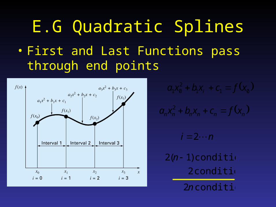
E.G Quadratic Splines• First and Last Functions pass through end

points

011201 xfcxbxa i

nnnnnn xfcxbxa 2

conditions )1(2 n

conditions 2

conditions 2n

ni 2

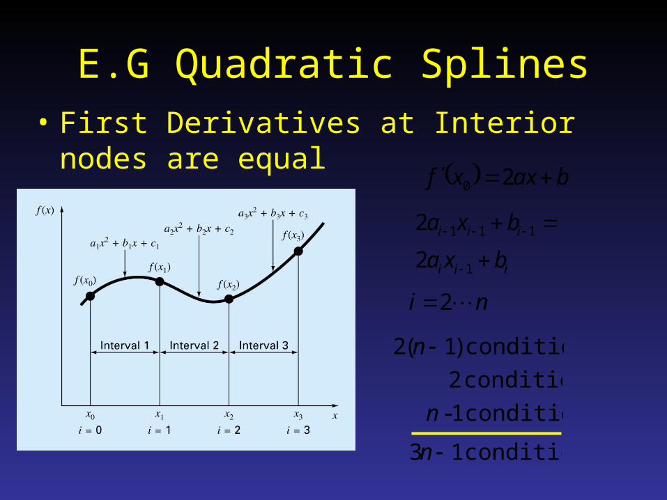
E.G Quadratic Splines• First Derivatives at Interior nodes are equal

baxxf 20

ni 2

conditions )1(2 n

conditions 2

conditions 13 n

iii

iii

bxa

bxa

1

111

2

2

conditions 1-n

E.G Quadratic Splines• Assume Second Derivative @ First Point=0

02 10 axf

conditions )1(2 n

conditions 2

conditions 3n

conditions 1-nconditions 1

E.G Quadratic Splines• Assume Second Derivative @ First Point=0

conditions 3n

tscoefficien edundetermin 3n

Solve 3nx3n system of Equations

baC

ix on based )( and

)( on based

xf

xf

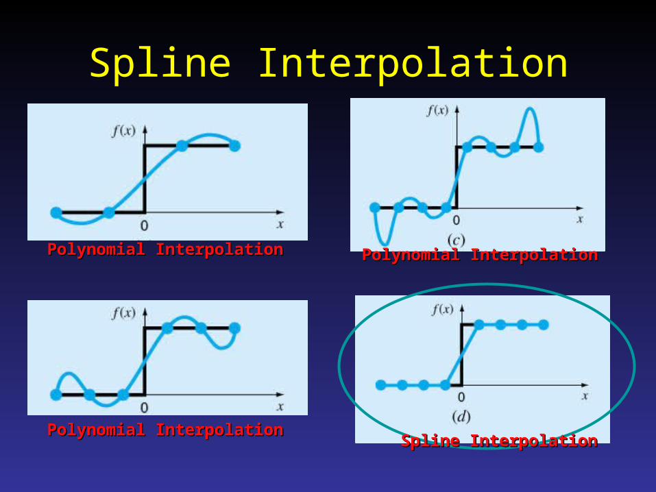
Spline Interpolation

Polynomial InterpolationPolynomial Interpolation

Spline InterpolationSpline InterpolationPolynomial InterpolationPolynomial Interpolation

Polynomial InterpolationPolynomial Interpolation