ESSAYS ON THE ECONOMIC IMPACTS OF

MOBILE PHONES IN SUB-SAHARAN AFRICA

By

Joshua Evan Blumenstock

A dissertation submitted in partial satisfaction ofthe requirements for the degree of Doctor of Philosophy in

Information Management and Systemsin the Graduate Division of the

University of California, Berkeley

Committee in charge:

Professor AnnaLee Saxenian, ChairProfessor John Chuang

Professor Alain de JanvryProfessor Edward MiguelProfessor Tapan Parikh

Spring 2012

Essays on the Economic Impacts of Mobile Phones in Sub-Saharan Africa

Copyright c© 2012, Some Rights Reserved (See: Appendix B)Joshua Evan Blumenstock

Abstract

Essays on the Economic Impacts of Mobile Phones in Sub-Saharan Africa

By

Joshua Evan BlumenstockDoctor of Philosophy in Information Management and Systems

University of California, Berkeley

Professor AnnaLee Saxenian, Chair

As mobile phones reach the remote corners of the world, they bring with them a sense of greatoptimism. Hailed as a technology that “can transform the lives of the people who are able to accessthem,"1 mobile phones have the potential to play a positive role in the lives of many of the world’spoor. Such claims are often reported alongside striking statistics on the uptake of mobile phonesin the developing world. Already, over two thirds of the world’s mobile phones are in developingcountries. In Nigeria, new subscribers are signing up for mobile phone services at a rate of almostone every second, and Nokia estimates that by the end of 2012 over 90 percent of sub-SaharanAfrica will have mobile coverage.2

This dissertation presents an empirical investigation of the role of mobile phones in Rwandansociety and economy. The material draws on two summers of field work in sub-Saharan Africa,several thousand interviews with mobile phone owners, and roughly ten terabytes of data on mobilephone use that I obtained from Rwanda’s largest telecommunications operator.

In the first chapter, I analyze the distribution of mobile technology within the Rwandan popula-tion, drawing attention to disparities in access to and use of mobile phones between rich and poor,and between men and women. The analysis highlights three sets of results. First, comparing thepopulation of mobile phone owners to the general Rwandan population, I find that phone ownersare considerably wealthier, better educated, and more predominantly male. Second, based on self-reported data, I observe statistically significant differences between genders in phone access anduse; for instance, women are more likely to use shared phones than men. Finally, analyzing thecomplete call records of each subscriber, I note large disparities in patterns of phone use and in thestructure of social networks by socioeconomic status.

The second chapter focuses on the economic implications of the spread of an early form of“mobile money" in Rwanda, and provides empirical evidence that this electronic currency is usedto transmit funds to individuals affected by catastrophic shocks. Contrasting two stylized modelsof prosocial behavior, this analysis provides insight into why people help each other in times ofdire need. The findings are based on the analysis of interpersonal interactions occurring immedi-ately before and after a destructive earthquake in Rwanda. The observed pattern of transfers is notconsistent with a model of pure charity or altruism, but better fits a model of risk sharing in whichindividuals mutually insure each other against uncorrelated income shocks.

The third and fourth chapters present methodological contributions, and serve to illustrate howmobile phone data can be used to observe and understand the behavior of populations in developingcountries, at a level of detail typically unobserved by social scientists. Chapter 3 develops a methodfor measuring levels and patterns of internal migration. After formalizing the concept of inferred

1‘Mobile phone lifeline for world’s poor’, BBC News, February 19 2007.2Statistics from United Nations (2007) and ‘Africa: Closing the Digital Divide’, allAfrica.com, February 16, 2009.

1

mobility, I compute this and other metrics for 1.5 million Rwandans, and provide novel quantitativeevidence consistent with qualitative findings by other scholars. Chapter 4 describes a new methodfor using mobile phone data to predict the socioeconomic status of an individual. The approachuses mixed methods and three distinct sources of data: anonymous call records; a governmentLiving Standards and Measurement Survey; and a set of phone surveys I conducted in 2009 and2010.

The chapters in this dissertation develop theory and methods for understanding how mobiletechnologies influence economic and social behavior, and how new sources of data can be used toprovide insight into patterns of human interaction. Taken together, the empirical results indicate thatphones have had a positive impact on the lives of some people but, absent intervention, the benefitsmay not reach those with the greatest need. The ultimate goal of these studies is to better understandhow information and communications technologies are changing, and can be used to improve, thelives of people worldwide.

2

This dissertation is dedicated to my parents, Ed Blumenstock and Belle Huang, forhelping me to get this far, and to my grandparents, Shing-Yi and Carrie Huang, and

Nathan and Paula Blum, for showing me what is important in life.

i

ii

CONTENTS

Acknowledgments . . . . . . . . . . . . . . . . . . . . . . . . . . . . . . . . . . . . . . v

1 Disparities in Access and Use of Mobile Phones in Rwanda 11.1 Abstract . . . . . . . . . . . . . . . . . . . . . . . . . . . . . . . . . . . . . . . . 11.2 Introduction . . . . . . . . . . . . . . . . . . . . . . . . . . . . . . . . . . . . . . 21.3 Related Work . . . . . . . . . . . . . . . . . . . . . . . . . . . . . . . . . . . . . 31.4 Data and Survey Methodology . . . . . . . . . . . . . . . . . . . . . . . . . . . . 41.5 Comparison of Phone Users to At-Large Population . . . . . . . . . . . . . . . . . 61.6 Reported Patterns of Phone Use . . . . . . . . . . . . . . . . . . . . . . . . . . . 91.7 Observed Patterns of Phone Use . . . . . . . . . . . . . . . . . . . . . . . . . . . 121.8 Discussion and Conclusion . . . . . . . . . . . . . . . . . . . . . . . . . . . . . . 14

2 Charity and Reciprocity in Mobile Phone-Based Giving 172.1 Abstract . . . . . . . . . . . . . . . . . . . . . . . . . . . . . . . . . . . . . . . . 172.2 Introduction . . . . . . . . . . . . . . . . . . . . . . . . . . . . . . . . . . . . . . 182.3 The effect of shocks on mobile phone-based transfers . . . . . . . . . . . . . . . . 202.4 Charity and reciprocity in interpersonal transfers . . . . . . . . . . . . . . . . . . 222.5 Data . . . . . . . . . . . . . . . . . . . . . . . . . . . . . . . . . . . . . . . . . . 252.6 Results . . . . . . . . . . . . . . . . . . . . . . . . . . . . . . . . . . . . . . . . . 312.7 Conclusion . . . . . . . . . . . . . . . . . . . . . . . . . . . . . . . . . . . . . . 432.8 Chapter Appendices . . . . . . . . . . . . . . . . . . . . . . . . . . . . . . . . . . 45

3 Inferring Patterns of Internal Migration from Mobile Phone Call Records 653.1 Abstract . . . . . . . . . . . . . . . . . . . . . . . . . . . . . . . . . . . . . . . . 653.2 Introduction . . . . . . . . . . . . . . . . . . . . . . . . . . . . . . . . . . . . . . 663.3 The challenge of measuring internal migration in developing countries . . . . . . . 673.4 How ICTs can provide better measures of migration and mobility . . . . . . . . . . 683.5 Case Study: Measuring internal migration and mobility in Rwanda . . . . . . . . . 693.6 Discussion . . . . . . . . . . . . . . . . . . . . . . . . . . . . . . . . . . . . . . . 783.7 Conclusion . . . . . . . . . . . . . . . . . . . . . . . . . . . . . . . . . . . . . . 82

4 A Method for Estimating the Relationship Between Phone Use and Wealth 854.1 Abstract . . . . . . . . . . . . . . . . . . . . . . . . . . . . . . . . . . . . . . . . 854.2 Introduction . . . . . . . . . . . . . . . . . . . . . . . . . . . . . . . . . . . . . . 864.3 Related Work . . . . . . . . . . . . . . . . . . . . . . . . . . . . . . . . . . . . . 864.4 Data . . . . . . . . . . . . . . . . . . . . . . . . . . . . . . . . . . . . . . . . . . 874.5 Methods . . . . . . . . . . . . . . . . . . . . . . . . . . . . . . . . . . . . . . . . 884.6 Results . . . . . . . . . . . . . . . . . . . . . . . . . . . . . . . . . . . . . . . . . 904.7 Limitations of our approach . . . . . . . . . . . . . . . . . . . . . . . . . . . . . . 92

iii

4.8 Conclusion . . . . . . . . . . . . . . . . . . . . . . . . . . . . . . . . . . . . . . 94

5 Conclusion 95

Bibliography 95

Appendices 105

A Survey Instruments 107

B Creative Commons License 127B.1 License . . . . . . . . . . . . . . . . . . . . . . . . . . . . . . . . . . . . . . . . 127B.2 Creative Commons Notice . . . . . . . . . . . . . . . . . . . . . . . . . . . . . . 131

iv

Acknowledgments

The material in this dissertation has benefited greatly from the insight and advice of my advisersand thesis committee: John Chuang, Alain de Janvry, Edward Miguel, and Tapan Parikh. I amdeeply indebted to my committee chair and mentor, AnnaLee Saxenian, for her continued supportover the past several years. I also gratefully acknowledge financial support from the InternationalGrowth Centre, the National Science Foundation, the Institute for Money, Technology and FinancialInclusion, the NET Institute, and Intel Research. Any errors, opinions, and conclusions expressedin this material are my own.

Finally, I give my heartfelt thanks to my family and friends for their love and encouragement.

Acknowledgments Specific to Chapter 1

I would like to thank Jenna Burrell, Tapan Parikh, Kentaro Toyama, and the three anonymous ref-erees for their thoughtful comments and suggestions. We are grateful to Santhi Kumaran and thefaculty and students at the Kigali Institute of Science and Techhnology for helping with the phonesurvey, and to Nadia Musaninkindi and Jean Marie Nyabyenda for their assistance with the DHSdata. Ye (Jack) Shen and Paige Dunn-Rankin provided excellent research assistance.

Acknowledgments Specific to Chapter 2

I am grateful for thoughtful comments from Alain de Janvry, Stefano DellaVigna, Frederico Finan,Mauricio Larrain, Ethan Ligon, Jeremy Magruder, Edward Miguel, Alex Rothenberg, ElisabethSadoulet, and seminar participants at NEUDC, PACDEV, MWIEDC, and the Berkeley DevelopmentLunch.

Acknowledgments Specific to Chapter 3

I gratefully acknowledge financial support from the National Science Foundation and the Inter-national Growth Centre. I would also like to thank Yian Shang for providing excellent researchassistance.

Acknowledgments Specific to Chapter 4

This study was funded in part by the Institute for Money, Technology, and Financial Inclusion, theNational Science Foundation, and the International Growth Centre. Paige Dunn-Rankin providedexcellent research assistance.

v

CHAPTER 1DISPARITIES IN ACCESS AND USE OF

MOBILE PHONES IN RWANDA

1.1 Abstract

This chapter provides quantitative evidence of disparities in mobile phone access and use in Rwanda.The analysis leverages data collected in 2,200 field interviews, which were merged with detailed,transaction-level call histories obtained from the mobile telecommunications operator. We presentthree related results. First, comparing the population of mobile phone owners to the general Rwan-dan population, we find that phone owners are considerably wealthier, better educated, and morepredominantly male. Second, based on self-reported data, we observe statistically significant differ-ences between genders in phone access and use; for instance, women are more likely to use sharedphones than men. Finally, analyzing the complete call records of each subscriber, we note largedisparities in patterns of phone use and in the structure of social networks by socioeconomic status.Taken together, the evidence in this chapter suggests that phones are disproportionately owned andused by the privileged strata of Rwandan society.1

1The material in this chapter is based on joint work with Nathan Eagle, originally published in 2012. See: Blumen-stock & Eagle (2012).

1

1.2 Introduction

Once the toys of rich yuppies, mobile phones have evolved in a few short years to be-come tools of economic empowerment for the world’s poorest people. These phonescompensate for inadequate infrastructure... making markets more efficient and unleash-ing entrepreneurship." - The Economist, September 2009

In the popular media, as well as in the development community, observers are optimistic aboutthe potential uses of the mobile phone in the developing world. Called a "lifeline for the world’spoor" by the BBC, mobile phones are reaching the world’s poor at an amazing rate (Anderson2007). Already, over two-thirds of the world’s mobile phones are in developing countries, andNokia estimates that, by 2012, more than 90% of sub-Saharan Africa will have mobile coverage(United Nations 2007).

The potential impact of the mobile phone has not been lost on the research community. Awealth of recent ethnographic research has sought to characterize mobile phone use in the develop-ing world, while a growing parallel body of quantitative work attempts to estimate the impacts ofthese technologies on local and national economies (Blumenstock, Eagle & Fafchamps 2011, Jensen2007, ?). A separate strain of research seeks to leverage this knowledge by designing mobile-basedtechnologies for deployment in developing countries (Brewer, Demmer, Ho, Honicky, Pal, Plauche& Surana 2006, Parikh, Javid, K, Ghosh & Toyama 2006).

Given this heightened interest in mobile phone use in developing countries, it is surprising howmany basic gaps exist in our understanding of how phones are being used on a day-to-day basis bythe average person. For instance, it is well known that many phones in East Africa are shared bymultiple individuals, but there are few reliable estimates regarding the overall prevalence of phonesharing. For this and other phenomena, even less is known about the subtler dynamics within thepopulation: Do women share phones more than men? Do they call a more diverse network ofcontacts? Do poor people use their phones differently from rich people?

This article seeks to fill a number of these gaps in our understanding through a detailed quan-titative analysis of phone use in Rwanda. The analysis is divided into three sections. First, wecompare the overall demographic composition of Rwanda with the demographic composition of arepresentative sample of mobile phone users, exposing systematic differences between those whoown phones and those who do not. Second, we examine new survey data on phone use, payingparticular attention to reported behaviors of phone ownership and sharing. Third, we analyze thecall histories of our survey respondents, as recorded by the mobile operator, to better understandnormal patterns of utilization. Some representative findings include the following insights:

• Section 1.5: Phone users are disproportionately male, better educated, and older, and theyalso come from larger households than normal Rwandans. Using an econometric model, weestimate the annual expenditures of phone users to be over twice that of ordinary citizens.

• Section 1.6: The vast majority of those surveyed report owning the phone they use, androughly one-third say they share their mobile phone with friends and family. We note statisti-cally significant differences between men and women in patterns of sharing and the types ofcalls made.

• Section 1.7: The length of the average call in Rwanda is extremely short, roughly 32 seconds.While men and women spend approximately the same amount of time per day on the phone,there are subtle differences in use by gender. We also observe vastly different patterns of usebetween the upper- and lower-income quartiles.

2

While the primary focus of this article is to provide a quantitative perspective on mobile phoneuse in Rwanda, we also contribute to the literature by describing a methodological innovation thatmay be useful to other researchers interested in studying information and communication technolo-gies (ICTs) in developing countries. This innovation is to combine data collected in structured phoneinterviews with the call detail records (CDR) that are logged by mobile phone operators. Thus, fora geographically stratified random sample of roughly 900 mobile phone users, we have obtainednot only basic demographic and socioeconomic information, but also a detailed history of all phonecalls made and received. Our analysis leverages this novel source of data, pointing to many possibleextensions for future work.

The remainder of the article is organized as follows: Section 1.3 discusses related work, andSection 1.4 describes the principal datasets used in the analysis. Section 1.5 presents a quantitativecomparison of the population of mobile phone users to the greater population of Rwandans. Sections1.6 and 1.7 analyze reported and observed patterns of mobile phone use, first using data collectedin phone interviews, and then incorporating the data obtained from the phone company. Section 1.8concludes.

1.3 Related Work

To our knowledge, this is the first article to study phone use through a joint analysis of large-scale household surveys, follow-up phone surveys, and call detail records (CDRs) obtained fromthe phone company. However, in addition to the review articles mentioned in the introduction, wehighlight the results of three separate strands of research that are directly relevant to the analysisthat follows.

First, a small group of studies has previously attempted to quantify patterns of phone use in thedeveloping world at a level of detail exceeding the cross-country statistics provided by organiza-tions such as the International Telecommunication Union. In particular, Gillwald (2005) conductedhousehold surveys in 10 African nations, in an effort to measure how individuals and householdsuse different types of ICTs. Using data collected in 2004 and 2005, the author supplies referencestatistics that provide a useful context for some of the numbers reported in this article. Separately,Scott, McKemyey & Batchelor (2004) conducted 1,800 household interviews in Uganda, Botswana,and Ghana, focusing on gender-disaggregated access to ICTs. They found that men and women hadremarkably similar patterns of use. By contrast, Huyer, Hafkin, Ertl & Dryburgh (2005) combineaggregate statistics from various sources to characterize the "gender divide" in access to, and useof, ICTs, finding women at a disadvantage with respect to several metrics of phone access and use.Our findings are generally more consistent with those of Huyer et al. (2005); we are also able tohighlight a number of gender-specific differences which, due to a lack of suitable data, were nottested in prior work.

Second, a nascent body of literature has begun to use CDRs to understand underlying dynam-ics of human behavior. For instance, Gonzalez, Hidalgo & Barabasi (2008) use CDRs to analyzethe trajectories of 100,000 people in a European country to study patterns of human mobility, andEagle, Pentland & Lazer (2009) examine the structure of friend networks using data from 100 spe-cially programmed smartphones. There are only a few examples of this type of analysis in thecontext of the developing world (Blumenstock et al. 2011, Blumenstock 2012, Blumenstock, Shen& Eagle 2010, Frias-Martinez, Frias-Martinez & Oliver 2010, Frias-Martinez, Virseda & Frias-Martinez 2010), but the number of studies is rapidly increasing as data become more readily avail-able.

Finally, there exists a handful of studies that provide excellent descriptions of different patterns

3

of mobile phone use in specific communities throughout the developing world (cf. Burrell 2010,Horst & Miller 2006), with a few focused specifically on Rwanda (Donner 2007, Futch & McIntosh2009). We draw on these insights in interpreting our quantitative results in the following sections.In particular, in the discussion and conclusion, we try to situate the quantitative results of this articlewithin the qualitative findings of researchers who have worked on similar questions.

1.4 Data and Survey Methodology

The analysis relies on three sources of data: a phone survey of a representative sample of Rwandanmobile phone users, a detailed log of all phone activity by those individuals in the period of Jan-uary 2005-December 2008, and a household-level demographic survey conducted by the Rwandangovernment. Further details on each dataset are provided in the following subsections.

1.4.1 Phone Survey

In the summer of 2009, employing a trained group of enumerators from the Kigali Institute ofScience and Technology, we administered a short, structured interview to a geographically strati-fied group of mobile phone users. The survey instrument contained roughly 80 questions and tookbetween 10 and 20 minutes to administer. We queried basic demographic and socioeconomic in-formation, but we did not collect identifying information, such as the respondent’s name, address,or identification numbers. The anonymized phone numbers were obtained from Rwanda’s primarymobile phone operator, which had over 90% market share at the time of the survey.

The survey population was intended to be a representative sample of all active phone users.Thus, from the full database of 1.5 million registered phone numbers, we eliminated numbers thathad not been used at least once in each of the three most recent months for which we had data(October-December 2008). Then, each one of the remaining 800,000 numbers was assigned to ageographic district based on the location of the phone for the majority of calls made. From each ofthe 30 districts, 300 numbers were selected randomly, creating a base survey population of 9,000candidate respondents, where sampling weights for each district were determined based on thedistribution of districts in the set of 800,000 active numbers. Given available resources, the team ofsurveyors was able to call 1,529 unique respondents who had been selected randomly from the poolof 9,000.

1.4.2 Phone Company Records

For each of the users whom we attempted to contact in the phone survey, we obtained from thephone company an exhaustive log of all phone-based activity that had occurred from the beginningof 2005 through the end of 2008. Thus, for every phone call made or received by one of the surveyrespondents, we had data on the time and date of the call, as well as the proximate location (based onthe cell towers through which the call was routed) of both the caller and the receiver. This allowedus to compute several metrics of phone use and social network structure for each of the 1,529 userswhom we attempted to contact. While most of the metrics we used are simple to understand andcompute, a few require explanation:

• Activation date: The date on which the phone first appears in the transaction logs.• Days of activity: The number of days on which the phone was used.• Net calls: The number of outgoing calls minus the number of incoming calls.• Degree: The number of unique contacts with whom the person communicated (called or

received a call).

4

• Daily degree: The average number of unique people contacted on any given day that thephone was used.• Recharge: Monetary value deposited on SIM card.

1.4.3 Rwanda Demographic and Health Survey

The final dataset we used is a large, representative household survey conducted by the Rwandangovernment in 2005. In the Demographic and Health Survey (DHS) of 10,272 households, detaileddata was collected on demographic composition, asset and durable ownership, and a wealth of othersocioeconomic indicators (de la Statistique du Rwanda (INSR) & Macro 2006). We used this datato compare the general Rwandan population to the population of phone users contacted in our phonesurvey.

1.4.4 Notes on the Data

Of the 1,529 numbers our surveyors attempted to dial, 588 (38%) never picked up the phone. Thelarge number of unanswered calls is striking, but not surprising. As has been noted by other re-searchers (James & Versteeg 2007), a large number of people own a SIM card (which costs roughlyUS$1) without actually owning a mobile phone (which costs closer to US$30). Moreover, SIMcards are commonly lost or stolen, and many people habitually leave their phones off due to the lackof reliable power in the country.

To the extent that these nonresponders are systematically different from responders, the externalvalidity of our results could be limited to the population of individuals likely to answer the phone,rather than the broader population of individuals who have ever used a phone. For instance, ifnonresponders tend to be poorer than responders, we might overestimate the wealth of the averagephone owner if we base our estimates solely on information provided by respondents.

However, the quantitative evidence at our disposal suggests that these biases are likely to besmall. For, although we were only able to collect demographic information for 901 respondents,we still have complete call usage information for the full sample of the 1,529 individuals whomwe attempted to contact, and we are therefore able to compare the usage pattern of respondentsto that of nonrespondents. We report these results in Table 1.1, where average values are com-puted separately for the set of numbers dialed (column 1), for survey respondents (column 2), fornonrespondents (column 3), and by response to this question: “Does anyone else use this phoneregularly?” (columns 4 and 5). The final two columns present the p-values obtained by runningtwo-sample t-tests comparing all respondents with all nonrespondents (column 6), and by compar-ing respondents who share their phone with those who do not share their phone (column 7).

In general, we observe only modest differences between the group of individuals who partici-pated in the phone survey and those who did not. In particular, on the days the phone is used (i.e.,activity “per day” in Table 1.1), behavior of nonrespondents is not statistically different from that ofrespondents. This is important, as we later assume that the sample of survey respondents is repre-sentative of the larger population of mobile phone users in Rwanda. However, the two groups are notidentical. Namely, there is a significant difference in the number of days the phone is used. Basedon the sum total of evidence presented in Table 1.1, we believe that the most likely explanation fornonresponse is that those individuals have discontinued use of their SIM card, either due to loss,theft, or replacement. An alternative explanation consistent with the data is that nonrespondents are,on any given day, less likely to use their phone, either because it is off, or because it is unavailable.However, the fact that respondents and nonrespondents act similarly when the phone is on (and inparticular, that they make the same number of calls and consume the same amount of airtime) pro-

5

vides some reassurance that the two groups are likely to be comparable along dimensions that, forpractical reasons, we are unable to directly observe.

Of those who answered their phones, only 16 (2%) refused to participate in the survey. Webelieve this very high response rate was due to several factors: First, incoming calls cost nothing toreceive, and respondents were paid US$1 in airtime as compensation, a significant amount, giventhat GDP per capita is roughly US$1,000. Second, most Rwandans are unaccustomed to receivinga call lasting up to 20 minutes (40 times the length of the average phone call), and many seemedflattered to receive the extended attention of university researchers. Finally, respondents were gen-erally more receptive than would be expected in most developed countries, where privacy concernsare rife.

After discarding a handful of surveys that had imperfect data, we were left with a total of 901valid surveys. The full breakdown of survey responses is given in Figure 1.1.

Figure 1.1: Survey population

Finally, it is also worthwhile to note that aggregate usage on shared phones does not appear tobe significantly different from aggregate usage on unshared phones (Table 1.1, column 7). This isuseful, as it allows us to increase our statistical power by including shared phones in most of thelater analysis. More generally, however, the result is surprising, as our expectation was that sharedphones would show both a higher level of use, and a wider network of contacts. The fact that sharedphones appear so similar to unshared phones could be due to a variety of factors: Non-owners mightbe using their own SIM cards; the owner of the shared phone might be the dominant user; or non-owners may use the phone in exactly the same way as the owner. These and other dynamics ofphone sharing are discussed further in Section 1.6.1.

1.5 Comparison of Phone Users to At-Large Population

Though mobile phone penetration has risen rapidly in Rwanda over the past decade, only roughlyone quarter of the population currently owns a mobile phone.2 While it is generally assumed thatthese phone owners are not representative of the population at large, the nature and extent of thesedifferences is not well understood. Here, we present a quantitative comparison of the representativepopulation of mobile phone owners, as captured in the phone survey, with the representative sample

2http://www.itu.int/ITU-D/icteye/, accessed December 2011.

6

Table 1.1: Summary statistics: Survey respondents, non-respondents, and shared phones.

(1) (2) (3) (4) (5) (6) (7)Dialed Respondents No Answer Shared Unshared RvN SvNS

Activation Date 2/9/08 1/12/08 4/5/08 1/2/08 1/12/08 - -Days of activity 672.2 770.3 540.3 702.3 799 0.0002 0.31Avg. call length 32.3 31.7 33 31.5 31.8 0.49 0.9Calls per day 6.24 6.25 6.23 6.32 6.22 0.98 0.94Net calls per day (out-in) 0.4 0.087 0.82 0.54 -0.1 0.19 0.46Degree 797.8 734.0 883.6 882.9 671.3 0.67 0.55Daily degree 3.81 3.78 3.86 3.98 3.7 0.91 0.72Int’l calls per day 0.09 0.084 0.099 0.083 0.084 0.53 0.97Credit used per day 184.6 163.5 212.9 151 168.8 0.3 0.62Max. recharge value 3391.6 2756.3 4246.4 2609.8 2818.3 0.28 0.62Calls per day (out) 3.32 3.17 3.52 3.43 3.06 0.63 0.69Calls per day (in) 2.92 3.08 2.71 2.89 3.16 0.28 0.58

N 1,529 901 628 239 661 - -

Notes: Mean values, weighted by sampling strata, are reported for all statistics except activation date, wherethe median is reported. Columns (6) and (7) report p-values from adjusted wald test for difference in meansbetween columns (2) and (3), and (4) and (5), respectively.

of the at-large population, as recorded in the 2005 household survey. For both samples, reportedstatistics are weighted by sampling strata.

1.5.1 Demographic Composition

We begin by analyzing the demographic composition of the two populations. The most strikingdemographic difference is in gender composition. While 47% of Rwandans are male, males ac-count for 67% of phone owners (see Table 1.2, panel A). Beyond gender, there are also significantdifferences in age, household size, and educational attainment. As is evident in Figure 1.2, the dif-ferences between phone users and the at-large population are systematic and occur throughout thedemographic distribution.

1.5.2 Socioeconomic Status

The demographic evidence seems to indicate that phones in Rwanda are owned primarily by the eco-nomically privileged. We now test this hypothesis directly. This test is not entirely straightforward,since, in practice, it is difficult to measure the socioeconomic status of a respondent, particularly ina short telephone interview. This difficulty arises because most Rwandans do not earn a fixed wage,and a large percentage of "income" is derived from home-produced goods or other informal chan-nels. Thus, we employ two separate means of measuring socioeconomic status: asset ownershipand predicted expenditures.

Asset ownership: In the Demographic and Health Survey (DHS), the Rwandan government col-lected data on a large number of indicators of wealth, such as housing characteristics and ownershipof assets and durables. We obtained the data and questionnaires used in the DHS, and we asked therespondents in our phone survey a subset of these questions verbatim. Panel B of Table 1.2 reportsthe average levels of asset ownership among phone survey respondents (column 1) and Rwandan

7

Table 1.2: Phone users vs. general populace(1) (2) (3)

Phone AllT-stat

Users Rwandans

Panel A: Demographic indicators

Age 32.03 21.37 32.03

Household size 5.87 4.98 11.56

Percent male 66.6% 47.4% 15.76

Completed sec. school 35.71% 1.60% 21.30

Panel B: Socioeconomic Status

Owns a car 19.1% 0.1% 6.35

Owns a bicycle 38.6% 12.9% 19.51

Owns a fridge 16.7% 1.2% 4.33

Owns a landline 2.8% 6.2% -17.33

Owns a radio 94.3% 52.9% 82.78

Owns a TV 39.4% 2.4% 12.53

Panel C: Expenditures

Predicted Expenditures $1,725 $753 24.05

Notes: Mean values reported, weighted by sampling strata. Col-umn (3) reports t-statistics testing for a difference in means be-tween columns (1) and (2). All differences are significant withat least 99.99% confidence. Predicted expenditures computedusing a conversion rate of RWF550=USD$1.

(a) Age (b) Household Size (c) Education

Figure 1.2: Demographic comparison of the population of mobile phone users to the population atlarge.

8

households measured in the DHS (column 2). The differences in asset ownership are stark, withphone users possessing a disproportionately large number of expensive assets. For instance, whileonly 2.4% of Rwandan households possess a TV, nearly 40% of phone users report TV ownership.

Predicted expenditures: The difference in asset ownership provides compelling evidence thatphone users are better off than the general population. However, the underlying differences inwealth and well-being are still murky. For instance, it is hard to say whether a person with a TVand a bicycle is better off than someone with a radio and a refrigerator. Thus, we derive a secondmeasure of socioeconomic status, predicted expenditures, that allows for a more direct comparisonof well-being along a single dimension of wealth. While the precise method for computing predictedexpenditures is described in a separate paper (Blumenstock, Shen & Eagle 2010), the basic idea is asfollows: First, actual expenditures are captured in the DHS through an exhaustive series of questionsabout household consumption. For the DHS sample, we can therefore compute total expenditures byaggregating expenditures across these subcategories in a manner following Deaton & Zaidi (2002).We then fit a model to the DHS data that relates total expenditures to asset ownership. The estimatedcoefficients of three models are presented in Table 1.3. We observe a strong relationship betweenasset ownership and total expenditures; using information on only eight attributes, the best modelexplains almost 60% of the variation in household expenditures. Finally, since each of these assetswas also measured in the phone survey, we can then predict the level of expenditures that wouldbe expected for each of the phone survey respondents, based on the assets already owned by therespondent.

In Table 1.2, panel C, we report the predicted annual expenditures for both populations, esti-mated with the above technique. Using the asset-based formula, we find that phone users have overtwice the predicted expenditures of ordinary Rwandans. As before, this difference is not idiosyn-cratic at the mean. As can be seen in Figure 1.3, the entire expenditure distribution is shifted to theright.

The aggregate socioeconomic differences between the two populations are notable, but theyshould be taken in the context of the limitations of the data. While Blumenstock, Shen & Ea-gle (2010) provide a more complete discussion of these limitations, we briefly note three sourcesof concern. First, our measure of predicted expenditures is crude and requires many problematicassumptions, particularly about the relationship between assets and expenditures (see Filmer &Pritchett 2001), and it glosses over distinctions among expenditures, consumption, and permanentincome (see Deaton & Muellbauer 1980). Second, there was a three-year interval between the timeswhen the government data was collected and the phone survey was conducted, during which mostRwandans experienced substantial improvements in socioeconomic status. Third, the data sets forthe two populations were collected with different methodologies, and the self-reporting bias in assetownership could conceivably be exaggerated in the phone survey. Whereas the government data wascollected by enumerators at the place of residence and could be verified visually, the data collectedover the phone could not be similarly confirmed. Despite these weaknesses, we believe the metricdoes provide a noisy indicator of socioeconomic status. In future work, we hope to do in-personfollow-up interviews with a small subset of respondents to gauge the magnitude of potential biases.

1.6 Reported Patterns of Phone Use

The previous section highlights the demographic and socioeconomic differences between averageRwandans and Rwandans with mobile phones. For the remainder of the article, we restrict our atten-tion to the population of mobile phone users, and focus on analyzing reported and observed patternsof mobile phone use. Reported behaviors are based on data gathered through phone interviews;

9

Table 1.3: Regression of Expenditures on Assets(1) (2) (3)

Assets + District FE + Livestock

HH size 0.115 0.123 0.110(31.20) (35.24) (26.94)

Car/Truck 0.650 0.661 0.545(8.12) (8.76) (4.81)

Bicycle 0.329 0.350 0.327(12.64) (13.65) (12.06)

Fridge 0.404 0.293 0.351(5.70) (4.40) (3.61)

Landline 1.055 0.800 0.779(28.97) (22.41) (15.66)

Goats 0.024(6.42)

Pigs 0.027(2.66)

Rabbits 0.005(0.99)

District FE NO YES YES

R2 0.520 0.577 0.487N 6900 6900 4739

Notes: Outcome is log of total household expenditures. T-statistics reported in parentheses. Regressions also includedmotorcycle, tv, radio, cattle, sheep, and chickens.

observed patterns are computed from the CDRs obtained from the phone company.

1.6.1 Ownership and Sharing

While most mobile phones in industrialized countries are owned and used by individuals, the situa-tion in developing countries is different (Steenson & Donner 2009). In East Africa, phone sharingis common. In Uganda, for instance, ethnographers have noted intricate social norms of sharingthat systematically exclude women and other subpopulations (Burrell 2010). Using the data fromthe phone survey, we can provide a quantitative perspective on these dynamics. Extrapolating fromthe representative survey to the larger population, we estimate that 30% of Rwandans share theirphone, where sharing is defined as an affirmative response to the question, “Does anyone else usethis phone regularly?” Of those who reported letting others use the phone, 42% reported that some-one else had used their phone in the last day, and 78% reported that someone had used the phone inthe last week. These and other statistics are presented in Table 1.4, panel A, column (1). Also worthnoting is the fact that nearly 98% of those surveyed reported that they owned the phone they wereusing. Taken in the context of the statistics on phone sharing, this leads us to believe that, regardlessof whether or not other people have access to a phone, it is the owner of the phone who typicallyanswers incoming calls from unknown callers.

Do these numbers match the observations of other researchers in similar contexts? The onlyother statistics we have seen on phone sharing in Rwanda estimate that between 2% and 70%

10

of people share their phones, but such a range is so large as to permit only minimal comparison(Nsengiyumva & Stork 2005). In other African nations, estimates of phone sharing tend to behigher, typically in the range of 30% to 70% (Gillwald 2005). However, given the large differencesin mobile access and ownership between nations, the numbers are hard to compare. Moreover, thedata in Gillwald (2005) was gathered in 2004, when fees were higher and mobile penetration waslower.

Table 1.4: Reported phone use(1) (2) (3) (4)All Men Women p-value

Panel A: Phone Ownership and sharingDo you own this phone? 97.87% 97.36% 98.87% 0.411Do you own another SIM card? 34.72% 35.42% 33.31% 0.806Does anyone else use this phone regularly? 29.67% 25.20% 38.55% 0.105

... How many different people used it in the last 24 hours? 0.73 0.74 0.71 0.925

... How many different people in the last 7 days? 2.15 2.37 1.87 0.362Panel B: Regular contactsRoughly how many times per week do you talk to...

... Friends (boy/girlfriend included) 20.85 25.42 11.76 0.002

... Family (spouse included) 11.02 9.99 13.06 0.323

... Business contacts 23.49 29.55 11.37 0.027Total calls per day (computed from above) 8.05 9.44 5.27 0.014Panel C: Types of calls madeHave you ever used your phone to...

... Seek help in an emergency? 26.82% 28.21% 24.06% 0.578

... Find a doctor? 31.07% 29.31% 34.57% 0.524

... Find a job? 45.22% 49.30% 36.83% 0.147

... Get advice on farming? 25.02% 27.21% 20.68% 0.308N 901 645 256 -

Notes: Percentages correspond to percent of affirmative responses (Panels A and C) or mean values(Panel B). All values weighted by sampling strata to produce averages representative of entire phonepopulation. Sharing within last 24 hours and 7 days is conditional on the phone being shared.

Columns (2), (3), and (4) of Table 1.4 highlight differences between genders with respect tophone sharing. In our representative sample, female respondents disproportionately reported thatthe phone was shared. However, this difference is only marginally significant, statistically. Alsonoteworthy is the fact that men and women report that a comparable number of different peoplehave used their phones in the past 24 hours or 7 days. This is likely due to the fact that both gendersreport that their spouse is the main other person to use the phone (38% for women, 43% for men).Finally, we observe modest differences in the gender composition of owners (22% female) vs. non-owners (37% female), but due to the small sample size of non-owners (19 of 901 respondents), thedifference is not statistically significant. We discuss the implications of this gender divide in Section1.8.

More generally, we checked a variety of other socioeconomic and demographic factors to seewhether any particular subpopulation was unusually likely to report using a shared phone. However,

11

phone sharing appeared to be evenly distributed across the population. For instance, we observedonly modest differences by geographic location. Similarly, a probit regression of phone sharing onour measure of predicted expenditures yielded a statistically insignificant coefficient. Finally, therewas no clear relationship between years of schooling and phone sharing, nor between householdsize and phone sharing.

1.6.2 Mobile Relationships

Finally, we asked all survey respondents about the people with whom they talk on the phone reg-ularly. Respondents were asked to estimate how many times in the past week they had spokento contacts in the following three categories: friends, family, and business. If the respondent wasunable to provide an estimate, the surveyor asked about the past 24-hour period, and multipliedthe response accordingly. Thus, the estimates are noisy because of measurement error and reportingbias, and also because many respondents did not draw clear distinctions among the different types ofcontacts. For instance, while the “family” category was relatively unambiguous, some respondentsfound our distinction between “friends” and “business contacts” to be somewhat contrived.

With these caveats in mind, we do note significant differences in the reported behavior of menand women. As can be seen in Table 1.4, panel B, men report a larger number of total calls, as wellas more frequent contact with friends and business contacts. Women, on the other hand, report morefrequent contact with family, though this last difference is not statistically significant. These trendsare generally consistent with qualitative observations of gender dynamics surrounding mobile phoneuse in developing countries. However, in other dimensions of phone use, the behavior of men andwomen appears similar (see Table 1.4, panel C). Unfortunately, our current analysis is limited bythe coarseness of the survey questions. In future work, we hope to further probe gender differencesin reported phone usage.

1.7 Observed Patterns of Phone Use

Until now, we have focused on the reported use of mobile phones, as described by the respondentsduring phone interviews. As has been noted previously, however, such data are likely to be noisyand biased. Fortunately, we have a more reliable measure of actual use: The call detail records(CDRs) obtained from the mobile operator provide an itemized list of all network activity for eachof our respondents. In Table 1.5, we summarize this usage using the same metrics as in Table 1.1.In addition, we compute the following:

• In/Out-degree: Number of different people to whom/from whom, calls were made/received.• Clustering: Percentage of first-degree contacts that have contacted each other.• Betweenness: Average shortest path between user and 50 randomly sampled numbers.• Me2U transfers: Interpersonal transfers of airtime made over the network.• Districts: Number of political districts in which the phone was used. Rwanda has 30 districts.

Aggregate statistics on phone use are presented in Table 1.5, column (1). The average Rwandancompletes 190 calls per month, each of which lasts an average of 32 seconds. It is difficult to findrecent, comparable figures from other countries, but both numbers are lower than the correspondingfigures are likely to be in most industrialized nations. For instance, estimates of use in the UnitedStates are closer to 204 calls per month, lasting roughly three minutes each; in India, the industryaverage is 377 minutes of use per month (Research 2006). These differences are most likely dueto the per-second fee structure and the high cost of a phone relative to daily income. To providesome context, a three-minute call in Rwanda costs roughly US$0.60, which amounts to 0.06% of

12

the average GDP per capita (GDPpc). The corresponding figure in the United States is US$0.60 fora three-minute call (0.001% of GDPpc); in India, a three-minute call costs only US$0.04 (roughly0.003% of GDPpc).

Table 1.5: Actual phone use, computed from transaction logs(1) (2) (3) (4) (5) (6) (7)All Men Women “Rich" “Poor" MvW RvP

Panel A: Domestic and International CallsActivation date 1/12/08 1/29/08 12/26/07 07/08/06 02/05/08 - -Days of activity 770.3 743.4 823.8 994.6 548.1 0.38 0.0001Avg. call length 31.7 29.7 35.7 39.8 28.4 0.014 0.0001Calls per day 6.25 6.32 6.09 8.42 6.47 0.82 0.26Net calls per day (out-in) 0.087 0.31 -0.37 0.76 -0.31 0.02 0.29Int’l calls per day 0.084 0.071 0.11 0.13 0.066 0.11 0.065Net int’l calls (out-in) -0.014 -0.0018 -0.038 -0.031 -0.028 0.031 0.89

Panel B: Social Network StructureDegree 734 772.6 657.2 1240.7 498.8 0.56 0.037In-degree 488.2 488.5 487.6 721.5 369.1 0.99 0.02Out-degree 433 475.9 347.7 798.1 280.8 0.43 0.1Daily degree 3.78 3.87 3.61 5.08 3.77 0.63 0.17Net daily degree (out-in) 0.00027 -0.17 0.34 -0.47 0.41 0.15 0.19Clustering 0.063 0.065 0.058 0.056 0.057 0.067 0.88Betweenness 2.72 2.74 2.69 2.61 2.77 0.27 0.0033

Panel C: Other BehaviorsCredit used per day 163.5 176.2 138.2 246.9 138.9 0.17 0.025Max. recharge value 2756.3 2775.1 2718.9 3816.1 2228.5 0.89 0.013Avg. districts per day 1.36 1.37 1.34 1.51 1.47 0.8 0.81Avg. districts contacted 1.21 1.2 1.22 1.4 1.28 0.81 0.48Me2U transfers per day 0.044 0.041 0.05 0.037 0.083 0.43 0.012Net Me2U transfers per day 0.00038 0.0066 -0.012 0.0082 -0.012 0.011 0.14

N 901 645 256 180 180 - -

Notes: Mean values reported, weighted by sampling strata to produce averages representative ofentire phone population. “Rich" and “poor" are defined as those respondents in the top and bottom20% of the predicted expenditure distribution, respectively. Columns (6) and (7) report p-valuesfrom adjusted wald test for difference in means between columns (2) and (3), and (4) and (5),respectively.

1.7.1 Differences by Gender

Within the sample of phone users, there are large differences in phone use across demographicgroups. In column (6) of Table 1.5, we highlight the differences between men and women. To sum-marize the results: Between genders, there are significant differences in the length of calls made(women talk longer), in the direction of the calls (women receive more calls than they make; menare the opposite), in international calling (both men and women receive more than they make, butwomen receive even more than men), and in airtime gifts using the Me2U service (women receivemore airtime). More broadly, men and women have comparably sized networks of contacts, but the

13

networks of men tend to be more tightly clustered than those of women. Finally, we note that, con-trary to the large and significant differences in total calls reported by male and female respondents(discussed in the previous section), the actual difference is small and statistically insignificant.

Given the impersonal nature of our metrics, it is not simple to interpret these statistics. Evidencefrom the United States and Norway suggests that gender differences in phone use are not unique todeveloping countries (Cotten, Anderson & Tufekci 2009, Ling 2001). Whether the differences seenin Rwanda reflect benign cultural differences or more insidious dynamics of power and patriarchyis a deeper question that we touch on in the conclusion.

1.7.2 Differences by Socioeconomic Status

While the differences by gender are somewhat ambiguous, the differences between socioeconomicgroups are striking. To analyze phone use by socioeconomic strata, we ranked each of the re-spondents by predicted expenditures – a measure based on known asset ownership, as discussed insection 1.5.2 – and then we separately computed averages for the upper and lower quartiles. Thesestatistics are presented in columns (4) and (5) of Table 1.5; the test for a difference between the twopopulations appears in column (7).

Above and beyond the differences between phone owners and non-owners (Figure 1.3), wenote large and consistent differences in usage within the population of owners, and in particular,between the richest 25% and the poorest 25% of phone users. Across nearly every measure, thericher people use their phones more: in number of calls, length of calls, number of days on whichthe phone is used, size and structure of the social network, etc. While some of these differences arenot statistically significant, the overall relationship between use and socioeconomic status remainsstrong.

1.8 Discussion and Conclusion

The preceding analysis provides a quantitative perspective on the demographic and socioeconomicstructure of mobile phone use in Rwanda. Though the analytic results are diverse, a relativelyconsistent picture begins to emerge: Mobile phone use in Rwanda is far from uniform. There aresignificant and systematic differences not only in who owns the phone (see Section 1.5), but also inhow different types of owners use the phone (see Sections 1.6 and 1.7). Specifically, phone ownersare much more likely to be male, they are better educated, they come from larger households, andthey are substantially wealthier than those without mobile phones. Within the population of phoneowners, there are differences in usage between men and women, particularly in reported phonesharing and the types of calls that are made. Most notable, however, is the vast difference in usebetween poorer and richer phone owners, such that the highest income quartile uses their phones30%-100% more than lowest income quartile, depending on the measure of use.

Taken together, the evidence in this article indicates that it is the privileged, male members ofRwandan society who disproportionately own and use mobile phones. Unfortunately, this patterndoes not seem to be unique to Rwanda; similar patterns have been observed in East Africa (Burrell2010) and other countries around the world (Huyer et al. 2005). Moreover, the same trends canbe seen with other technologies in other contexts. For instance, Toyama, Kiri, Menon, Pal, Sethi &Srinivasan (2005) and Kiri & Menon (2006) observe that use of telecenters is dominated by younger,more educated men.

The preceding analysis to be useful for a few distinct reasons. First, we believe there is intrinsicvalue in developing insight into the daily patterns of use of such a massively popular technology, in

14

part to help scholars and practitioners better understand how phone-based technologies are likely tobe received and used. As we have seen, traditional Western models of phone use-and the potentialdesign assumptions they impose-do not necessarily apply to the Rwandan context. Second, we hopeour methods and analysis can inspire and be improved on by other researchers. In particular, themethod of coupling anonymous call detail records with structured phone interviews should providefertile ground for future work. Finally, by providing more reliable estimates of the distribution ofphone access and use, we seek to inform policy makers about the potential distributional impacts ofphone use in countries such as Rwanda. Given the considerable attention and investment devotedto mobile telephony in developing countries, it is important to better understand who is-and whoisn’t-reaping the benefits of the new technology.

15

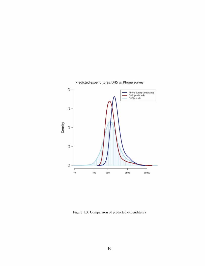
Figure 1.3: Comparison of predicted expenditures

16

CHAPTER 2CHARITY AND RECIPROCITY IN MOBILE

PHONE-BASED GIVING

2.1 Abstract

We provide empirical evidence that an early form of “mobile money” is used to transmit funds toindividuals affected by catastrophic shocks. Contrasting two stylized models of prosocial behavior,we further provide insight into why people help each other in times of dire need. Our findings arebased on the analysis of billions of mobile phone-based transactions that occur before and after adestructive earthquake in Rwanda. The observed pattern of transfers is not consistent with a modelof pure charity or altruism, but better fits a model of instrumental reciprocity. This conclusion issupported by three distinct results. First, earthquake-induced transfers are increasing in the wealthof the recipient, and are not significantly related to the wealth of the sender. Second, transferssent in response to the earthquake are highly dependent on the prior history of transfers. Third,transfers decrease as the distance between sender and recipient increases, even after controlling forthe strength of pairwise relationships. Taken together, the evidence indicates that Rwandans use themobile phone network to help afflicted friends and family, but that these gifts are motivated, at leastin part, by a desire for reciprocity.1

1The material in this chapter is based on joint work with Nathan Eagle and Marcel Fafchamps. See: Blumenstocket al. (2011).

17

2.2 Introduction

Why do people help each other in times of dire need? Economists typically ascribe two broadmotives for prosocial behavior: charity, where a giver gives out of the desire to improve the welfareof his friend; and reciprocity, where gifts are embedded in long-term relationships of reciprocalexchange. While these motives may be reasonable under ordinary circumstances, during timesof real crisis it seems likely that charity would prevail. As Adam Smith observed, humans arefrequently moved by pity and compassion, by “the emotion which we feel for the misery of others,when we either see it, or are made to conceive it in a very lively manner” (Smith 1759, p.3). Whensomeone really needs help, aren’t we all capable of setting aside self-interest and acting purely outof charity or altruism?

Understanding the motives for pro-social behavior is of primary concern in developing economies,where informal gifts and in-kind transfers play a critical role in enabling individuals and householdsto smooth consumption in the presence of temporary economic shocks (Udry 1994, Townsend 1994,Jalan & Ravallion 1999). Such knowledge not only provides insight into an important feature ofmany traditional societies, but can inform policies designed to promote sharing and ameliorate risk(cf. Cox 1987, Goetz & Gupta 1996).

In a developing country context, much of the theoretical literature assumes that interpersonal orinterhousehold transfers are realized in a repeated game of mutual insurance with limited commit-ment (cf. Coate & Ravallion 1993, Kocherlakota 1996, Ligon, Thomas & Worrall 2002). The resul-tant risk sharing networks, while effective at insuring against uncorrelated, idiosyncratic shocks,are less effective against large, covariate shocks that affect entire communities simultaneously(Townsend 1995).2 While altruism has long been known to play an important role in facilitatingrisk sharing (Becker 1991, Foster & Rosenzweig 2001, Fafchamps & Lund 2003, Platteau, Kolm& Ythier 2006), it is typically quite difficult to empirically differentiate altruism from other factorsthat may affect risk sharing arrangements.

In this paper, we examine the motives governing pro-social behavior in response to large,publicly-observable economic shocks. Empirically, we exploit a comprehensive dataset of mo-bile phone-based activity that we obtained from the primary telecommunications operator in theRwanda. We observe over 50 billion mobile phone transactions over a four year period, includingroughly 10 million person-to-person transfers of mobile airtime, a precursor to the “mobile money"networks that are now quite common in many developing countries.3 Our results are identified bya major earthquake that occurred in early 2008 and devastated the Western Lake Kivu region of thecountry.

We begin by providing empirical evidence that, in the immediate aftermath of the earthquake,people from all over Rwandan transferred funds to individuals living close to the epicenter. Whilethe effect is small in absolute terms (we estimate that between $25,000 and $33,000 would be

2In a world of complete information, enforceable contracts, and negligible transaction costs, these informal arrange-ments could be sustained over long distances and individuals could in principle receive support from outside the com-munity. However, real-world risk sharing is plagued by information asymmetries (Attanasio & Pavoni 2011), problemsof limited commitment (Thomas & Worrall 1990), and transaction costs (Jack & Suri 2011). Thus, the overwhelmingbody of empirical evidence indicates that in-kind and monetary transfers typically occur between friends and familywithin small, local communities (Udry 1994, Fafchamps & Gubert 2007, Kurosaki & Fafchamps 2002, de Weerdt &Fafchamps 2010).

3As of late 2010, “branchless banking" systems had been deployed in over 80 countries worldwide (McKay & Pickens2010). A common feature of many of these systems is a transfer mechanism that allows subscribers to transfer moneyor airtime balance to another subscriber’s account instantaneously. In Kenya, over US$200 million is transferred overthe system per day (Pulver 2009). In Rwanda, the system is less sophisticated, and initially only permitted interpersonaltransfers of airtime. In late 2010, the system was expanded to allow for over-the-counter purchases and other monetarytransactions.

18

sent in response to a current-day earthquake), it is statistically highly significant. Moreover, wesuspect that the marginal utility benefit of the transfer is due less to infra-marginal savings on airtimeexpenditures than it is to enabling a stricken individual to communicate with loved ones or reliefworkers. Indeed, most Rwandans carry a near-zero balance on their mobile phones, so the infusionof even a small amount of airtime could have a meaningful impact at a time of distress.

In our second set of results, we investigate the motives that cause people to transfer funds tothose affected by the earthquake. Here, we seek to differentiate between two stylized models ofmobile phone-based giving. In the first “charity-based” model, we assume that the utility functionof an individual i is linearly dependent on the utility of his partner j (Becker 1974, Andreoni & Miller2002). This model – as well as related models of Fehr & Schmidt (1999), Charness & Rabin (2002),and Andreoni (1990) – predicts that transfers increase in the wealth of the sender and decrease inthe wealth of the recipient. In the second “reciprocity-based” model, we adopt the framework ofrisk sharing under dynamic limited commitment first proposed by Ligon et al. (2002). Buildingon the insights of Foster & Rosenzweig (2001) and Ligon (1998), this model predicts that shock-induced transfers are dependent on the past history of transfers between i and j, and on the costsof monitoring and enforcing contracts. Alternative formulations of reciprocity, and in particular themodels of intrinsic, preference-based reciprocity (cf. Rabin 1993, Falk & Fischbacher 2006), yieldsimilar predictions.

We then compare these empirical predictions to the actual patterns of transfers observed in thedata. Contrary to our expectation, we find evidence that pure charity is not the sole determinant ofearthquake-induced transfers. Instead, the data are more consistent with reciprocal motives. Threepieces of evidence support this interpretation. First, it is the wealthier individuals who receive thelargest volume of transfers in the immediate aftermath of the earthquake, not the poorer individualsas the charity model predicts. Second, there is a strong history-dependence of transfers sent in re-sponse to large shocks. An individual i is significantly more likely to receive from j in the immediateaftermath of the earthquake if i sent funds to j prior to the earthquake, or if the “net balance" of thepast transfers that i received from j is negative, i.e., i has given more to j than he/she received. Thirdand finally, post-quake transfers decrease with the geographic distance between i and j, even whencontrolling for the strength of the relationship between i and j.4 While such an effect is expectedwhen geographic distance limits commitment, it is not expected if transfers are purely charitable,given the absence of transaction fees and the publicly observed nature of the earthquake. In allspecifications, we account for possible confounding factors by including dyad fixed effects, timedummies, and time-varying controls.

The evidence presented in this paper thus indicates that Rwandans are using the mobile phonenetwork to help each other cope with large covariate shocks, and that these transfers appear to bedriven, at least in part, by reciprocal motives. This finding is consistent with recent work by Jack &Suri (2011), who utilize household surveys to show that Kenyans with access to mobile money arebetter able to smooth consumption than those without.

This research contributes to, and helps synthesize, two well-established literatures on pro-socialbehavior and risk sharing. The distinction we draw between charitable and reciprocal motives israther coarse in comparison to recent behavioral experiments that can distinguish between differ-ent types of charity, such as pure vs. impure altruism, and different types of reciprocity, such asintrinsic vs. instrumental reciprocity (c.f. Leider, Mobius, Rosenblat & Do 2009, DellaVigna, List& Malmendier 2011, Ligon & Schechter 2011, Cabral, Ozbay & Schotter 2011). While our use of

4We control for social proximity in two ways. First, we count the total number of phone calls between i and jover a period of time prior to the earthquake. Second, we measure the “network flow" (Karlan, Mobius, Rosenblat &Szeidl 2009) by counting the total number of unique paths between i and j in the call graph.

19

observational data limits our ability to perform this decomposition, our approach has the advantageof providing insight into prosocial behavior in response to events of dire consequence. As discussedmore extensively by Levitt & List (2007), it can quite be difficult to recreate in an experimentalsetting the feelings and behaviors elicited by real-world catastrophes. Our in situ analysis is morecommon in the literature on risk sharing, but such empirical analysis is typically constrained bya lack of reliable data on interpersonal transfers. As a result, most studies have either relied onsmall samples, self-reported behaviors of subjects, or both (e.g. Fafchamps & Gubert 2007, Jack &Suri 2011). In our study, we observe a complete census of millions transfers – some of which aresent in response to exogenous shocks – and can examine the motives behind in situ risk sharing.

These findings also contribute to a growing body of research concerned with understandingthe economic impact of mobile phones and other information and communication technologies(ICTs) in developing economies. Recent work in this area describes how mobile phones can reduceinformation asymmetries (Jensen 2007), lower search costs (Aker 2008), lower transaction costs(Jack & Suri 2011), and enhance communication with government agents (Shapiro & Weidmann2011). Our analysis indicates that, unlike traditional risk sharing networks, where the vast majorityof transfers occur within small, local communities, a majority of the mobile-phone based transferscome from outside the region affected by the quake.5 By relaxing geographic constraints to risksharing, mobile money enables a wider set of potential remitters. While this is generally a positivedevelopment, we note that there is considerable heterogeneity in who benefits from access to thenetwork: wealthy individuals, and individuals with larger and more geographically disperse socialnetworks, are most likely to receive a transfer after a severe shock.

Finally, we make two methodological contributions that can facilitate the use of similar large-scale, network-based datasets in social science research. First, we develop a novel method forestimating the permanent income of a mobile phone subscriber based solely on the history of phonecalls and the structure of the call graph. Second, we develop a locational inference algorithm thatallows us to impute the location of an individual based on the routing of his calls through the physicalnetwork of mobile phone towers.

The remainder of the paper is organized as follows. Section 2.3 describes our empirical strategyfor measuring the extent to which the mobile phone network in Rwanda is used to transfer fundsto people affected by severe economic shocks. In Section 2.4, we present two stylized models ofcharity and reciprocity, show that these models produce divergent empirical predictions, and outlinethe strategy we will use to test these models with the data. The data and the algorithms used toprocess them are described in Section 2.5. We present our empirical results in Section 2.6, alongwith several robustness checks. Section 2.7 concludes.

2.3 The effect of shocks on mobile phone-based transfers

In October of 2006, the monopoly mobile phone provider in Rwanda launched a rudimentary “mo-bile money" system that allowed mobile subscribers to transfer airtime from one person to another,free of charge. The first objective of this paper is to test whether this network was used to trans-

5In traditional risk sharing networks, Udry (1994) observes that 75 percent of surveyed Nigerian households madeinformal loans, but that almost all loans occurred within a village. Fafchamps & Gubert (2007) similarly observe thatgeographic proximity is a major determinant of sharing patterns: when two households live near each other, it is morelikely that the one will help the other. Kurosaki & Fafchamps (2002) and de Weerdt & Fafchamps (2010) obtain similarfindings for Pakistan and Tanzania, respectively. See Rosenzweig & Stark (1989) for somewhat contradictory evidencefrom India.

20

fer airtime to individuals affected by idiosyncratic economic shocks.6 To identify our results, weexploit the exogenous variation in transfers driven by unpredictable economic shocks, and in partic-ular a destructive earthquake. Our empirical model estimates the extent to which individuals livingin areas unaffected by such shocks send airtime to individuals close to the epicenter.

We measure this response at three levels: at the regional level (district and cell tower); at thelevel of individual subscribers; and at the level of dyads, where each dyad is formed by a directedpair of two subscribers. From a policy point of view, the regional analysis is perhaps the mostrelevant: it allows us to quantify the total value of transfers received by the affected region, and thusprovide a sense of the aggregate welfare benefit that was achieved.

It does, however, matter whether airtime transfers were broadly distributed across the popula-tion, or only reached a happy few. For this reason, we disaggregate transfers to the level of individualsubscribers in order to analyze heterogeneity of effects. This allows us to ascertain which types ofindividuals are most likely to receive shock-induced transfers. Finally, because we are interested notjust in the types of individuals that receive transfers, but also the types of relationships that supportinterpersonal transfers, we further disaggregate transfers at the level of pairs of users – or dyads.As we discuss in the following section, it is the dyadic- and individual-level analysis that allows usto differentiate between motives for prosocial behavior. Combining these two types of analysis isseldom possible because researchers typically only have either aggregate or survey data. We have acensus of all transfers and can thus look at all levels simultaneously.

Formally, let τi jrt denote the gross transfer of airtime received by an individual i, located inregion r at time t, from another individual j. Further define τirt = ∑ j τi jrt the total gross transfersreceived by user i in region r at time t, and define τrt = ∑i τirt as the total gross transfers receivedby users in location r at time t. We estimate models of the form:

τrt = α1 + γ1Shockrt +θt +πr + εrt (2.1)

τirt = α2 + γ2Shockirt +φNearE picenterit +θt +πi + εirt (2.2)

τi jrt = α3 + γ3Shockirt +φNearE picenterit +θt +πi j + εi jrt (2.3)

where Shockrt is a dummy variable equal to 1 if location r received a shock on day t, and Shockirt

equals 1 if i was near the epicenter at the time of the shock.7 θt is a vector of time dummies, andπr,πi, and πi j are fixed effects for the region, individual, and dyad, respectively. NearE picenterit ,which indicates whether i was in the area affected by a shock on day t (irrespective of a shockoccurring), controls for the possibility that individuals might receive transfers when visiting the areaaffected by the earthquake. In regression (2.2), individuals i who never receive airtime transfers areexcluded since they do not help identify γ2. In regression (2.3), pairs of individuals (i, j) that arenever observed to transfer money to one another are similarly omitted. Time dummies θt controlfor long-term growth in traffic, as well as day-of-the-week (e.g., week-end) and day-of-the-month(e.g., payday) effects that affect all regions similarly. Location and recipient fixed effects πr and πi

control for the fact that different locations or users are more likely to receive transfers on average.Dyadic fixed effects πi j control for the average intensity and direction of transfer flows between twousers. Finally, to minimize the likelihood that our results are driven by differential growth in mobile

6More recently, the Rwandan telecommunications provider significantly expanded the capabilities of this mobilemoney system to allow for bill payment, point-of-sale transactions, re-conversion of credit to cash, and (soon) interest-bearing savings accounts. During the period of time we analyze, however, credit could only be used to make phone calls,though it was quite common to exchange airtime for cash at retail locations. In Section 2.6, we discuss the extent towhich these restrictions affect our interpretation of the quantitative results.

7Technically, Sirt is the interaction between NearE picenterit and DayO f Shockt , a dummy variable that takes the value1 on the day of the shock (for all i) and zero otherwise. The uninteracted variable DayO f Shockt is observed by the timedummies θt and omitted for clarity.

21

usage across locations, we restrict the analysis to a specific time window Tmin ≤ ts ≤ Tmax aroundthe time of the shock ts.

Identification is achieved as in a difference-in-difference framework: parameters γ1,γ2 and γ3represent the average treatment effect of the shock on people with access to the mobile moneynetwork. The exogeneity of Shockrt is guaranteed since its timing could not have been predicted,i.e., the shock constitutes a natural experiment. If γ1 > 0,γ2 > 0 and γ3 > 0, this is interpretedas evidence that the shock Shockrt caused an increase in airtime transfers to users in the affectedregion. We check the robustness of our results in various ways, notably by varying the time windowover which the models are estimated, by controlling for several factors that depend on both time andlocation, and by running a number of falsification and placebo tests. Following Bertrand, Duflo &Mullainathan (2004), in individual and dyadic regressions standard errors are clustered by location(i.e., by the location of the nearest cellular tower).

2.4 Charity and reciprocity in interpersonal transfers

A primary objective of the paper is to provide insight into the motives behind transfers that are madein response to a publicly observed shock. Since our data are observational, and since the identitiesof the mobile subscribers are unknown, we are somewhat constrained in our ability to impute whatare fundamentally personal decisions. Thus, we stop short of recent experimental work that, throughclever manipulation of experimental conditions, can differentiate between instrumental and intrinsicreciprocity (Ligon & Schechter 2011, Cabral et al. 2011, Leider et al. 2009, Charness & Rabin2002). Instead, we follow Leider et al. (2009) and divide the motivations for prosocial behaviorinto two rough categories which, for short, we call ‘charity’ and ‘reciprocity.’8 In this section,we develop stylized models of charity and reciprocity, derive comparative statics, and describe theidentification strategy we will employ to differentiate between the two models.

2.4.1 Theoretical Framework

Charity

By charity we refer to the broad class of motives where a giver gives because he receives directutility from the act of giving or from increasing the utility of another. The canonical example ofthis behavior is pure altruism (Becker 1976, Andreoni & Miller 2002), where one person’s utilitydepends positively on another’s:

Uit = ui(xit − τ jit)+ γi ju jt(x j + τ jit) (2.4)

As before, we denote by τ jit a transfer sent to i from j at time t. Assuming ui(·) and u j(·) areincreasing and concave, with xi representing the income of individual i and γi j denoting the level ofaltruism felt by i toward j, it is easily shown that two predictions of such a model are

∂E[τ ji|xi]

∂xi≥ 0 and (2.5)

∂E[τ ji|x j]

∂x j≤ 0 (2.6)

8Our distinction also parallels the distinction Ligon & Schechter (2011) draw between “preference-related" motivesand “incentive-related" motives.

22

Giving is expected to increase in the income of the sender (as the marginal cost of giving decreases),and decrease in the income of the recipient (as the marginal benefit of a gift decreases). Such pre-dictions are supported by observed patterns of altruism in a variety of contexts, including charitablegiving in the United States (Andreoni 2006) and the behavior of “rescuers” in Nazi-occupied Europeduring World War II (Hoffman 2010).

While the comparative statics (2.5) and (2.6) are most transparent in the model of pure linearaltruism specified by equation (2.4), similar predictions obtain from several related models of char-itable behavior, and we make no pretense to be able to distinguish between them. Thus, models ofinequity and inequality aversion (where i seeks to minimize |xi−x j|), social welfare models (wherei maximizes min{x1, ...,xn}), and warm glow giving (where v(x j + τ ji) in (2.4) is replaced withτ ji) all yield similar predictions (cf. Fehr & Schmidt 1999, Bolton & Ockenfels 2000, Charness &Rabin 2002, Andreoni 1990, List & Lucking-Reiley 2002).

Defining charity thus broadly, it follows that if the primary motive for transfers is a charitableone, we expect transfers on average to come from richer users and to flow to poorer users. In casesof directed altruism, where γi j varies across dyads, we expect transfers to decrease with the socialdistance between i and j, but conditional on social distance, there is no a priori reason to expecta relationship between transfers and geographic distance. Similarly, after controlling for socialdistance, charitable transfers should be “memory-less" (Fafchamps & Lund 2003), and past transfersshould not directly influence transfers sent in response to shocks. To the extent that an associationdoes exist between past transfers and current transfers, we would expect it to be positive, as pasttransfers may reveal information about how much i cares about j, above and beyond the undirectedmeasures of relationship strength that we employ.

Reciprocity

By reciprocity, we refer to motives that are embedded in long-term relationships of bilateral ex-change. In the discussion that follows, we focus on a particular type of instrumental reciprocity,where mutual exchange is motivated by the expectation of future reciprocation (cf. Coate & Ravallion1993, Karlan et al. 2009). This model most transparently leads to empirical predictions that can betested with the data at our disposal. Other models of reciprocity, and most notably the intrinsic,preference-based reciprocity modeled by Rabin (1993) and Falk & Fischbacher (2006), producesimilar predictions. Since our intent is not to differentiate between these different types of reci-procity, we present a simple model of dynamic limited commitment that captures many of the centraltenets of the wider literature.9

We adopt a model of risk sharing under dynamic limited commitment, developed by Ligonet al. (2002) and Foster & Rosenzweig (2001). Following Foster & Rosenzweig (2001), we assumei has stationary, single-period utility specified by (2.4), but allow for the possibility that i expects tobenefit from future interaction with j:

Uit = ui(xit − τ jit)+ γi ju j(x jt + τ jit)+E∞

∑s=t+1

δs−t [ui(xis− τ jis)+ γi ju j(x js + τ jis)] (2.7)

The first part of (2.7) is identical to the altruistic model (2.4), while the second term captures thediscounted expected utility of the relationship.

This formulation produces two key insights relevant to the current analysis. First, when con-tracts are not fully enforceable ex-post, transfers received in the current period will depend on past

9For recent experimental work that differentiates between different types of reciprocity, see Leider et al. (2009), Ligon& Schechter (2011), and Cabral et al. (2011). Fehr & Schmidt (2006) and Sobel (2005) provide theoretical overviews.

23

transfers given. This property is formally derived in Appendix 2.8.1, however the intuition is quitesimple: In the stationary model of (2.4), i and j will transfer the necessary τ jit to equate the ratioof their ex post marginal utilities to γ (or 1/γ if xi < x j). If γ is sufficiently small, i and j operatein autarky. By contrast, in the dynamic model specified by (2.7), i and j also derive utility fromexpected future interactions and transfers, and so may adjust the ratio of marginal utilities at timet to maintain the relationship and avoid reversion to a series of static Nash equilibria. Intuitively,when i suffers a shock in period t, the marginal utility of τi jt will be quite high and so he will bewilling to sacrifice a greater share of his continuation utility in exchange for a larger transfer at t.As a result, we expect transfers from i to j sent in response to a shock to be decreasing in the netbalance of transfers previously made from i to j (denoted by T net

jit ):

∂E[τ jit |T netjit ]

∂T netjit

≤ 0 where T netjit =

t−1

∑s=0

τ jis− τi js (2.8)

As robustness checks, we further expect that τ jit will decrease in the gross volume of prior transfersfrom i to j (denoted by Tjit) and increase in gross prior transfers from j to i (denoted by Ti jt):

∂E[τ jit |Tjit ]

∂Tjit≤ 0 where Tjit =

t−1

∑s=0

τ jis (2.9)

∂E[τ jit |Ti jt ]

∂Ti jt≥ 0 (2.10)

Empirically, this dynamic model of limited commitment explains the data better than a stationarymodel with no history-dependence (Ligon et al. 2002, Genicot & Ray 2003, Fafchamps & Lund2003).

The second insight of our model of risk sharing under limited commitment, also discussedextensively in Ligon (1998) and De Vreyer, Gubert & Roubaud (2010), is that transfers wouldbe expected to decrease as, ceteris paribus, the cost of monitoring and enforcement increases. Inthe context of our study, it is natural to assume that monitoring costs increase monotonically withgeographic distance Di j. For instance, if j wants to verify the damage to i (e.g., injury, destroyedbuilding), j has to travel to the affected area, and the cost of travel increases with distance. Thus, ifthe need to monitor constrains transfers, we expect that:

∂E[τi j|di j,Si j]

∂di j≤ 0 (2.11)

i.e., the further away j resides from i, the more costly it is to verify the effect of the shock on i, andthe harder it is to overcome j’s fear of being cheated.

Of course, distance is likely correlated with other factors that influence the decision to give, butwhich are not related to monitoring and enforcement per se. For instance, transaction costs, whichoften rise with distance, have received recent attention by Jack & Suri (2011). However, since thecost of remitting over Rwandan mobile is free at all distances, transaction costs are unlikely to driveempirical estimates of (2.11). More generally, when we operationalize (2.11) in a regression setting,we will always condition our empirical results on Si j, an undirected measure of the strength of therelationship between i and j, and a dyad fixed effect πi j, so that we estimate the partial effect ofgeographic distance holding constant other unobservable characteristics of the dyad.

Unlike the model of charity, the model of reciprocity does not make strong predictions regardingthe relative wealth of i and j. We might expect transfers to go to wealthier individuals if strategicagents seek to ingratiate themselves for future reciprocation. Such an interpretation is supported

24

by recent work by Schechter & Yuskavage (2011), who find that transfers are likely to flow frommore to less wealthy households in unreciprocated relationships, while reciprocated relationshipsare more likely between wealthier households. Alternatively, we could observe flows from the richto the poor if the poor reciprocate in ways other than airtime (Fafchamps 1999, Platteau 1995).

2.4.2 Identification and Estimation

Table 2.4 summarizes the empirical predictions of the two stylized models of mobile phone-basedgiving. If, as seems reasonable to expect under such exigent circumstances, transfers given inresponse to severe shocks are motivated by feelings of charity, they should be increasing in thewealth of the sender and decreasing in the wealth of the recipient. However, conditional on thestrength of the relationship between sender and recipient there should be no marginal impact ofthe geographic distance between partners, or the past history of transfers. On the other hand, iftransfers are embedded in relationships of reciprocity, then the relative wealth of the two individualswould have an ambiguous effect on transfers. The key determinants instead are the past history oftransfers between individuals and the geographic proximity. Both models predict that transfers willbe increasing in social proximity.

To test these predictions empirically, we estimate heterogeneous effect models of the form:

τit = α2+ γ2Shockit +β2ZiShockit +φ2NearE picenterit +

η2ZiDayO f Shockt +ζ2ZiNearE picenterit +θt +πi + εit (2.12)

τi jt = α3+ γ3Shockit +β3Zi jShockit +φ3NearE picenterit +

η3Zi jDayO f Shockt +ζ3Zi jNearE picenterit +θt +πi j + εi jt (2.13)

where Zi and Zi j are vectors of characteristics associated with individuals and pairs of individuals(dyads). The regressions are used to estimate the partial effects described in Table 2.4. As be-fore, Shockit takes the value one if i is affected by the shock and zero otherwise. Shockit is theproduct of DayO f Shockt , a dummy variable taking the value one on the day of a severe shock andNearE picenterit , a dummy variable indicating whether i was close to the shock on day t. Doubleinteraction terms of the form ZiDayO f Shockt are included to control for the possibility that, in thecountry as a whole, variation in Zi affects transfers on the day of the shock differently from otherdays.

We are primarily interested in using models (2.12)-(2.13) to differentiate between charity andreciprocity by testing the effects of Zi j = {xi,x j,Si j,Di j,T net

i j } on transfers sent in response to severeshocks. In the following section, we describe the data used in the analysis, our technique for mea-suring the various components of (2.1)-(2.3) that are necessary to estimate the average treatmenteffect, and our method for measuring wealth, past transfer history, geographic distance, and socialconnectedness.

2.5 Data

The main dataset used in this paper comes from Rwanda’s primary telecommunications operator,which until recently held a near monopoly on mobile telephony in the country.10 The data contain a

10During the window of time we examine, the operator we focus on maintains over 90% market share of the mo-bile market. The company’s primary competitor did not gain traction in the market until the end of 2008, and onlyvery recently has the market become competitive. The number of landlines in Rwanda is insignificant (roughly 0.25%penetration).

25

comprehensive log of all activity that occurred on this network between early 2005 and late 2008. Intotal, we observe detailed information on over 50 billion transactions (including calls, text messages,and airtime transfers and purchases), covering 1.5 million users over four years. Summary statisticsof this dataset are given in Table 2.1.

During the four-year period for which we have data, uptake of mobile phones was extremelyrapid. In early 2005, only 2.5 percent of Rwandans owned a mobile phone, but by 2010 mobilepenetration had increased to 33.4 percent (a compound annual growth rate of roughly 74 percent).11

Such rapid growth is common in many sub-Saharan Afrian nations, where landlines are rare and thecost of owning a mobile phone is falling quickly.12

2.5.1 Interpersonal Transfers

Our empirical analysis focuses on interpersonal transfers of airtime credit between mobile sub-scribers. These transfers are made possible by a rudimentary “mobile banking" system that waslaunched in October 2006. After purchasing airtime from a local vendor, mobile subscribers areable to send that airtime to another subscriber, instantaneously and free of transaction fees. Duringthe period of time we analyze, the system only allowed for transfers of airtime, and there was noofficial mechanism that allowed for conversion of airtime back into cash. In 2010 the phone com-pany greatly expanded the capabilities of the system to allow for over-the-counter transactions, billpayments, and other debit account-like services. Following the trend in much of the developingworld, where over 1.7 billion people own a mobile phone but do not have a bank account (CGAPand GSMA 2009), most Rwandans did not have access to formal financial services in early 2008.As can be seen in Table 2.2, compared to other available mechanisms for sending funds, the mobilemoney system is considerably cheaper, faster, and easier to access.

In our dataset, we observe detailed information on roughly 10 million interpersonal transfers ofairtime. For each transaction, we know the date, time, and value of the transfer, as well as a unique(anonymized) identifier for both the sender and recipient. To estimate the regressions describedin sections 2.3 and 2.4, we aggregate this raw data on each day for each region (equation 2.1,individual (equation 2.2), and dyadic pair of individuals (equation 2.3). This allows us to measure,at three different levels of aggregation, the net and gross volume of airtime received on each day.Summary statistics of the dataset are provided in Table 2.1.

2.5.2 Locational Inference

The identification strategy we employ relies on spatial, as well as temporal, variation in transfers.Therefore, it is important that we be able to assign each individual, on each day, to an approximategeographic location. The mobile phone operator records information on the location of each in-dividual at the moment a call is initiated or terminated, and the only record kept is of the nearestcellular tower, not the actual GPS coordinates of the subscriber. As can be seen in Figure 2.1, whichshows the spatial distribution of cell phone towers in early 2008, towers in rural areas are relatively

11Source: International Telecommunications Union. http://www.itu.int/ITU-D/ICTEYE/Reports.aspx, ac-cessed November 2011.

12Though prices are falling, the cost of mobile telephony are still relatively high and represent a significant portion ofhousehold expenditures (Ureta 2005). In Rwanda it costs roughly $50 for the phone, and an additional $0.20 per minuteand $0.10 per SMS (see Republic of Rwanda (2010) and Donner (2008)). The ITU estimates the monthly “price basket"for mobile service to be $12.30 per month, which is based on the prepaid price for 25 calls per month spread over thesame mobile network, other mobile networks, and mobile to fixed calls and during peak, off-peak, and weekend times.The basket also includes 30 text messages per month (http://devdata.worldbank.org/ict/rwa_ict.pdf).

26

Table 2.1: Summary statistics of mobile network data.

Dates covered All dates Earthquake window

10/1/2006-7/1/2008 1/3/2008-3/3/2008

Panel A: Aggregate traffic

Number of Calls 46,000,000,000 868,786,684

Number of interpersonal transfers 9,202,954 362,053

Number of unique users 1,084,085 119,745

Number of people who send airtime 870,099 48,295

Number of people who receive airtime 946,855 101,351

Number of people who both send and receive 732,869 29,901

Number of unique dyads 646,713 159,204

Panel B: Basic statistics (12/1/2007-4/1/2008) Mean S.D.

Transactions per user (send+receive) 6.05 12.05

Average distance per transaction (km) 13.51 27.67

Average transaction value (RWF) 223.58 652.02

Notes: The window 10/1/2006-7/1/2008 encompasses the entire dataset with valid data on interpersonal airtime

transfers. The window 1/3/2008-3/3/2008 is the same window used in later regressions. US$1=550RWF.

Table 2.2: Formal services for transferring money in Rwanda, c. 2008

Service Estimated Fees(small transfers)

Availability Source

Mobile Phone Free 3 million phones

MoneyGram 7% - 100%($15 minimum)

5 locations MoneyGram Website, 2010

Western Union 10%-100%($10 minimum)

Approx. 50 locations Western Union Website,2010

Post Office 8%-50% 19 branches World Bank Group (2009)

Commercial Bank 6%-40% Only in urban, semi-urban areas

World Bank Group (2009)

Public Bus 6% - 20% Populous areas Avg. for Bus-Star, Scandi-navian Transportation

Notes: Data compiled in August 2010 from sources listed in column 4. See Orozco (2009) and Kabbucho,

Sander & Mukwana (2003) for further quantitative estimates, or Collins, Morduch, Rutherford & Ruthven

(2009) for a more general overview.

27

sparse, so being able to locate individuals between towers can potentially improve the precision ofour models.13

Figure 2.1: Map of Rwanda showing the location of mobile phone towers (as of February 2008) andthe location of the Lake Kivu earthquake of 2008. Each black dot represents a cell tower, with theapproximate area covered by the tower demarcated by adjacent Voronoi cells. The epicenter of theearthquake is shown with red concentric circles.

To solve this problem, we develop a locational inference algorithm that allows us to approximatethe continuous trajectory of each user through time and space, based on the intermittent sequence ofphone calls logged by the mobile operator. The method utilizes a kernel function K(·) to estimatean unknown location at time t from the kernel-weighted Euclidean centroid of known locations attimes in the vicinity of t (cf. Blumenstock 2012).

Formally, we estimate the unknown location rit of individual i at time t as

rit =1

Nit

Tmax

∑s=Tmin

K(t− s

h) · qis

where Nit is the total number of phone calls made by i within a window of time [Tmin,Tmax] sym-metric around t, and qis is the (known) location of the tower used at time s. K(x) is a symmetricfunction that integrates to one, which specifies the extent to which additional weight is placed on

13the median area covered by a single cell phone tower is 72km2. Note that cellular coverage is not affected by topologyto the same extent as radio transmitters as in Yanagizawa-Drott (2010).

28

Figure 2.2: Map of Rwanda showing a single individual’s inferred trajectory over a 6 month period.Although the individual only makes a small number of phone calls, the locational inference algo-rithm is able to roughly assign the user a continuous trajectory through time to places not restrictedto the set of known locations of cellular towers. This particular individual is observed to slowlymigrate southeastward, with early locations colored dark red and later locations colored yellow.

calls close in time to t. In our results we use a uniform kernel such that K(u) = 1/Ni, however verylittle changes if a different kernel is specified.

2.5.3 Characteristics of individuals and dyads

To differentiate between the models of charity and reciprocity described in Section 2.4, we measurecharacteristics of individuals and dyads Zi j = {xi,x j,Si j,Di jt ,T net

i jt } as follows.Social connectedness (Si j): Both models predict that transfers will increase in the strength of

the relationship between i and j, so measurement of this effect does not contribute directly the theorywe hope to test. However, since certain components of Zi j may be correlated with Si j (notably Di jt

and Ti j), controlling for Si j directly can bias. We measure Si j in two ways: first, following Marmaros& Sacerdote (2006) we simply calculate the total number of non-monetary interactions (phone callsand text messages) between i and j in the N days prior to t. Second, building on the insight ofKarlan et al. (2009), we additionally measure the maximum network flow as the number of distinctpaths between i and j in the complete undirected call graph.

Past transfer history (Ti jt): Since we observe all transactions between i and j over a 4-yearperiod, it is possible at any point t to compute the gross balance of payment sent from j to i as

29

Ti jt =∑s<t τi js and from i to j as Tjit =∑s<t τ jis. The net balance of transfers T neti jt is simply Ti jt−Tjit .

Geographical distance (Di jt): To estimate the distance between i and j at time t, we first com-pute the (latitude,longitude) locations rit = (φi,λi) and r jt = (φ j,λ j) using the locational inferencealgorithm described in Section 2.5.2. Then, we compute the arc distance Di jt using the haversineformula:

Di jt = 2r · arcsin

(√sin2

(∆φ

2

)+ cosφi cosφ j sin2

(∆λ

2

))where ∆φ = |φi−φ j|, ∆λ = |λi−λ j| and r = 6356.78 is the radius of the earth.

Wealth (xi and x j): While the preceding metrics are straightforward to compute, it is consid-erably more difficult to measure the wealth of each individual since all users in the dataset appearanonymously and without demographic information such as the age, gender, education level, ordirect proxies for socioeconomic status. Instead, we construct a crude proxy of each individual’swealth by combining detailed call data with regionally-tagged data from a household Demographicand Health Survey and follow-up phone interviews conducted in Rwanda in 2009 and 2010. We pro-vide a concise description of this method here; the reader is referred to Appendix 2.8.3 for furtherdetails.

1. Using a 10,000-household Demographic and Health Survey (DHS) that contains detailed con-sumption and expenditure information (Government of Rwanda, 2008), we first estimate ahedonic regression of annual expenditures Yid of household i in district d on fixed assets Aidand housing characteristics Hid .

Yid = α+hmax

∑j

β jHid +amax

∑k

δkAid +µd + εid (2.14)

The quantities Yid , Aid , and Hid are all captured in the DHS, and µd is a district fixed effect.Equation (2.14) predicts the annual expenditure Yid of a household on the basis of easilyobservable Aid , and Hid . We regard Yid is as a proxy for permanent income.

2. Next, we use data from a phone survey to relate Hid and Aid to phone usage. The survey,conducted by the authors, covers a geographically stratified random sample of approximately2,000 mobile subscribers. For each individual, we collected basic demographic information,together with data on Hid and Aid . Armed with Hid and Aid , it is possible to compute predictedannual expenditures Yid for the 2,000 mobile subscribers using the coefficient estimates fromequation (2.14).

3. Finally, we compute, for each phone user, a vector of phone usage variables Xir thought tobe correlated with income, such as the total number of calls made and the average amountof airtime purchased over a given time interval (we exclude information on airtime transfersto minimize potential endogeneity). A subset of these variables are summarized in AppendixTable (2.16). We then fit a flexible model of the form:

Yid = f (Xir) (2.15)

and estimate f (.) using data from the phone user survey. Our wealth index is the predictedY id obtained by applying the estimated flexible function f (.) to the full sample of 1.5 millionphone users. This variable is used as proxy for wealth or permanent income when estimatingheterogeneous effect equations (2.12) to (2.13). Details on f (·), as well as potential endo-geneity concerns, are discussed at length in Appendix 2.8.3.

30

2.6 Results

Our identification strategy requires a shock Shockrt that is exogenous to transfers on the mobilephone network. The primary shock that we exploit is a large earthquake that occurred in the WesternRusizi and Nyamasheke districts of Rwanda on February 3, 2008. The magnitude 6 earthquake left43 dead and 1,090 injured. It destroyed 2,288 houses and caused regional school closures andelectrical outages (though only one cell tower of 267 was affected). The effects of the earthquake,though large, were geographically circumscribed. The United States Geographical Survey estimatesan impacted radius of approximately 20 kilometers from the epicenter – see Figure 2.1. Based onnews reports and discussions with individuals in Rwanda, it does not appear that any particulardemographic subgroup of the population was disproportionately affected by this earthquake, and inparticular, rich and poor households appear to have been similarly affected (USGS 2009).14 Thisevent is ideal for our estimation strategy since the shock is unequivocally exogenous and preciselylocated in time and space. We later demonstrate that our results are robust to using alternative shockmeasures including a severe flood that occurred in late 2007.

We begin by estimating models (2.1)-(2.3) to measure the causal impact of the earthquake oninterpersonal transfers. We then turn to models (2.12) and (2.13) to measure heterogeneity and testthe models of charity and reciprocity presented in Section 2.4.1.

2.6.1 Average effect of the earthquake

Baseline results

We first estimate equation (2.1) at the regional level, and present the results in Panel A of Table 2.3.The dependent variable τrt is the total value of transfers received on day t by region r. Column 1defines r at the level of the political district (of which there are 30); column 2 defines r at the levelof the cell tower (of which there are 267). While the district-level specification may seem morenatural, the advantage of the tower-level results is that each observation corresponds to a smallergeographical unit and thereby allows us to more precisely identify the regions affected by the quake.In all specifications, we use data from 30 days before to 30 days after the earthquake, though asdemonstrated in 2.6.1 results our results change little if we use a different time window. Region andday fixed effects are included as additional regressors to control for systematic differences acrossdistricts and over time. The earthquake shock variable Shockrt equals one on February 3rd 2008, theday of the earthquake, in regions affected by the earthquake.15 Robust standard errors are reported,clustered at the district level.

We are primarily interested in the coefficient on “Earthquake Shock," which indicates the extentto which an anomalous volume of mobile airtime was sent to regions affected by the earthquake. Inall specifications the estimate is highly significant, with T-statistics between 7 and 16.

Columns (3) and (4) repeat the estimation at the level of the individual user and of the dyadicpair of individuals. In column (3), the dependent variable τirt is the amount of airtime transfered toindividual i in location r at time t. Users who never receive airtime transfers are excluded since theydo not help identify the effect of the shock, leaving roughly 110,000 unique individuals. Resultsfrom the dyad-level regression (2.3) are presented in column (4) of Table 2.3. In this regression,

14Much of the damage was sustained in and around the semi-urban city of Cyangugu, where a relatively representativesubset of the population resides. See, for instance, http://earthquake.usgs.gov/eqcenter/eqinthenews/2008/us2008mzam/

15For the district-level specification, affected regions are the districts of Rusizi and Nyamasheke. For the tower-levelspecification, it is towers within 20km of the epicenter, though similar point estimates and standard errors are producedif we redefine affected areas as those lying anywhere between 10 to 50 miles of the epicenter.

31

Table 2.3: Average Effect of the Earthquake on Transfers Received

(1) (2) (3) (4)

District Cell Tower User Dyad

Panel A: Gross transfers received (total incoming)

Earthquake Shock 14,169.2*** 2,832*** 9.48*** 8.14***

(1,951.3) (177) (0.74) (1.34)

NearE picenterit 1.26*** 0.23*

(0.19) (0.11)

Unconditional Mean 19,006.9 2,436.2 5.90 3.65

Unconditional Mean (affected area) 6355.9 1245.3 3.8 3.2

Panel B: Net transfers received (incoming - outgoing)

Earthquake shock 12822.58*** 3053*** 10.01*** 8.816***

(1599.87) (116) (1.08) (1.65)

NearE picenterit 0.58 0.45+

0.46 (0.24)

Unconditional Mean 0 0 0 0

Unconditional Mean (affected area) 1398.51 248.38 0.514 0.64

Panel C: Total cost of calls received

Earthquake Shock 2,501,220** 565,329** 247.95*** –

(886,529) (168,349) ( 34.21) –

NearE picenterit -22.17*** –

(5.89) –

Unconditional Mean 3,845,858 425,740 162.91

Unconditional Mean (affected area) 1,843,455 353,501 154.17

Number of observations 1,800 16,020 6,619,440‡ 10,032,721

Day dummies Yes Yes Yes Yes

Fixed effects District Tower Individual Dyad (Directed)

Notes: In Panels A and B, the dependent variable is the gross (Panel A) and net (Panel B) transfers received on a givenday by a given district (column 1), cell tower (column 2), individual subscriber (column 3), or by an individual i froma specific individual j (column 4). In Panel C, the dependent variable is the total amount of money spent to call thedistrict/tower/subscriber on each day. The Earthquake Shock variable takes the value one for regions/subscribers whowere within 20km of epicenter on the day of the earthquake; NearE picenterit takes the value one for all observationswhere the subscriber is within 20km of the epicenter (even when there is no earthquake). The unconditional mean reportsthe average of the dependent variable across the entire 2-month window (January 4 2008 - March 3 2008), for the countryas a whole and for the region affected by the earthquake. ‡ Column (3) of Panel C includes all phone subscribers, not justindividuals who had used the mobile money service, and includes 35,539,241 observations. We do not estimate column(4) of Panel C because the roughly 100 billion observations made the computation infeasible. Standard errors, clusteredby district, reported in parentheses. ∗ significant at p < .05; ∗∗p < .01;∗∗∗p < .001.

32

pairs in which i never receives airtime from j are ignored from the estimation, leaving roughly180,000 valid dyads. At both levels, the Shockirt coefficient is positive and statistically significant.The evidence is thus consistent: at all levels of aggregation we observe an increase in gross transfers.

Interpretation

Do these effects matter? Based on the coefficient estimate in column (2) of Table 2.3, we observethat the earthquake produced an additional influx of approximately 42,000 RWF (or $84 U.S. Dol-lars) to the 15 towers within 20km of the epicenter. This amount is small in absolute terms, butRwanda is a small country of ten million people, and only 50,000 people lived in the region af-fected by the earthquake, of whom no more than 7 percent owned a mobile phone at the time ofthe earthquake.16 Based on the data at our disposal, we know that only 1,400 individuals livingin the earthquake region had used the service prior to January 2008. If the net influx were evenlydistributed among these eligible users (which it wasn’t - most transfers were sent to a lucky few),each individual would have received roughly 30 RWF (about five cents).

If the sole benefit of this transfer were an infra-marginal savings on future airtime expenditures,then the utility gain would indeed be quite small. However, as can be seen in Figure 2.3, mostRwandans carry very little airtime on their account. At midnight the night before the earthquake,the median balance for the entire population of phone users was only 49.4 RWF, and roughly 32percent of all subscribers had an airtime balance of less than 5 RWF. Thus, the marginal utility of30 RWF to someone who had just experienced an earthquake is potentially quite large – it wouldhave been sufficient to make a short phone call or send a text message, to call for help or to simplyreassure a loved one.17 In the immediate aftermath of several recent natural disasters, mobile phoneshave been instrumental in facilitating rescue attempts, though we have no direct evidence of thisoccurring after the Lake Kivu earthquake.18

To further put these numbers in context, it is worth noting that since the earthquake, service uti-lization has increased over 400-fold. As of early 2011, there were between 750,000 and 1,000,000active mobile money users in Rwanda each day. This compares to 2,500 at the time of the earth-quake. If we were willing to assume that airtime transfers following an earthquake would increaseproportionally to the number of active users, a similar earthquake today would be expected causean additional influx of US$25,000 to $33,000 to affected areas.19 In neighboring Kenya, where thepopulation is much larger and the local mobile money service is more widely used, the daily vol-ume of money transferred over the mobile phone network is in excess of US$200 million, comparedto US$1,500 in Rwanda at the time of the quake. If we were willing to assume that emergency

16It is difficult to estimate the total population affected by the earthquake, however Cyangugu, the largest city inthe region, has a population of roughly 20,000. Mobile phone penetration in Rwanda was roughly 7 percent in 2008,but a disproportionate share of owners live in the urban capital of Kigali, and penetration rates outside the capital aresignificantly lower (Blumenstock, Gillick & Eagle 2010).

1730 RWF would also have been sufficient to enable a Rwandan to send a “missed call" (also referred to as a flash ora beep) to a friend, which is a common way of signaling that the caller wishes to talk but does not want to pay for thecost of a call. Sending missed calls in Rwanda in 2008 required that the subscriber have a positive balance on his or heraccount.

18For a recent example, see “In Turkey, Desperate Race to Find Trapped Survivors”, New York Times, October 25,2011: “Some dug with their bare hands, while other used heavy machinery to remove chunks of fallen concrete and reliedon cellphone calls from the missing in the search for survivors... a 19-year-old in the town survived by using his cellphoneto direct teams to the collapsed building where he had been trapped."

19 750,0002,500 ∗$84 = $25,200. If these transfers are proportional to traffic and traffic increases non-linearly in the number

of subscribers, as much of the network literature suggests, the projected amount may even be much larger. It is also con-ceivable, however, that early adopters are not representative of late adopters and respond more strongly to an earthquake;in this case, transfers need not increase proportionally with traffic or the number of users.

33

Figure 2.3: Distribution of end-of-day account balances on February 1, 2008, the day before theLake Kivu earthquake. Subscribers with balances in the top and bottom 0.5 percent of all userswere removed to improve the display of the histogram (one user had a balance of 442500RWF).

34

transfers would increase proportionally to the total volume of airtime transfers, we would expect aninflux of approximately US$11.2 million ($84 ×200M/1500) to affected regions.

Robustness

As a robustness check, we redo the same analysis using net instead of gross transfers. The concernis that gross transfers may misrepresent the aggregate magnitude of the transfers if individuals whoreceive airtime pass it on to others in the same region. This could result in double-counting atthe district or cell tower level. For the individual user regression (2.2) we redefine the dependentvariable as τ′irt = ∑ j τi jrt−∑ j τ jirt , that is, the transfers received by i from others minus the transfersgiven by i to others. At the district and cell tower levels, we proceed as follows. Let τr1r2t =

∑i∈r1 ∑ j∈r2 τi jrt where r1 and r2 are two different locations (e.g., districts or cell tower area); τr1r2t

represents the total transfers received by individuals in location r1 from individuals in location r2.Summing over all other locations yields the gross transfers from other locations to location r1. Netinflows to region r1 are thus τ′r1t = ∑r2 τr1r2t −∑r2 τr2r1t . Results, shown in Panel B of Table 2.3 aresimilar in significance and magnitude to those reported in Panel A, implying that the magnitude ofour findings is not driven by double counting.

In Appendix 2.8.2, we present several additional robustness checks to ensure that our results are(i) not sensitive to the econometric specification, (ii) do not depend on the choice of time window,and (iii) are not affected by the structure imposed on the variance matrix. In addition, we run a seriesof “placebo” tests to demonstrate that similar results do not obtain on days where no earthquakeoccurs. Finally, to demonstrate that the effects observed in response to the Lake Kivu earthquakeare likely to generalize to other severe shocks, we show that a similar, albeit muted, response isobserved after a series of large floods that occurred in late 2007. The reader is referred to Appendix2.8.2 for further details on these tests.

2.6.2 Differentiating between charity and reciprocity

Our next task is to test whether the pattern of transfers observed following the Lake Kivu earthquakeis more consistent with a model of charity or of reciprocity. As a starting point, we note that thevast majority of pairwise relationships we observe do not exhibit a strong reciprocal component. Ofthe 646,713 dyadic pairs (i, j) for which a transfer is observed in one direction (from either i to j orj to i), transfers are observed in both directions in only 143,394 dyads (22 percent). However, forthe subset of dyads that respond to the earthquake, that ratio jumps to 31 percent. This difference,which is statistically significant, suggests that the quake-induced transfers are embedded in long-term reciprocal relationships.

To test these intuitions more formally, we introduce heterogeneous effects into our analysis.As summarized in Table 2.4, we have proposed three indirect tests: (i) Wealth: if transfers aremotivated by charity, they are expected to flow from wealthier to poorer individuals; not necessarilyso if they follow a reciprocal motive. (ii) History-dependence: Ceteris paribus, charitable transfersshould not depend on history; however, if transfers are embedded in reciprocal relationships, shock-induced transfers should exhibit history-dependence as characterized by equations (2.8)-(2.10). (iii)Geographic distance: Transfers motivated by reciprocity are expected to decrease with distance, butconditional on the strength of the relationship between i and j, charitable transfers should exhibitno such dependence.20

We focus on the individual and dyadic regression models (2.12) and (2.13), where the vector

20Of course, individuals who are themselves affected by the earthquake are less likely to be in a position to assist,

35

Table 2.4: Summary of predictions and results

Predicted

Partial Interpretation Charity Reciprocity Observed

∂τi jt/∂xi Wealth of i (recipient) Negative – Positive

∂τi jt/∂x j Wealth of j (sender) Positive – –

∂τi jt/∂Si j Social connectedness of i and j (recipient) Positive Positive Positive

∂τi jt/∂Di jt Geographic distance between i and j at time t – Negative Negative

∂τi jt/∂T neti jt Net balance of transfers from j to i (Positive) Negative Negative

Notes: Summary of predictions of stylized models of charity and reciprocity presented in Section 2.4.1, and

results described in Section 2.6. Parentheses indicate weak predictions.

of covariates Zi j includes the measures of xi,x j,Si j,Di j, and T neti j discussed in Section 2.5.21 Re-

gression results are presented in Tables 2.5-2.6. As before, we include data from 30 days before to30 days after the earthquake (January 4, 2008 through March 3, 2009), and compute Zi j using datafrom 2007. In all specifications we include a vector of daily fixed effects and interactions betweenZi j and DayO f Quaket and NearE picenterit , though these coefficients are omitted from most tablesfor clarity of presentation. In our preferred specification (column 1), we additionally include indi-vidual and pairwise fixed effects πi j to reduce potential bias from time-invariant omitted variables.However, inclusion of these fixed effects makes it impossible to estimate the unconditional effectof Zi j on τi j, i.e., whether certain characteristics make transfers more likely on non-shock days.Thus, we follow Wooldridge (2005) and separately recover the average partial effects by obtainingthe predicted τi j from (2.13) and then regressing these predicted values on Zi j (column 2). We alsoinclude specifications with no fixed effects as a point of reference, though as noted these estimatesare likely to be biased (column 1). In all specifications, we include a full set of interactions betweenSi j and Shockit , in order to reduce the potential bias that other factors correlated with Zi j (such ashow much i and j like one another) are spuriously driving the effect we attribute to Zi j. The measureSi j used in our main specifications is simply the total number of phone calls observed between i andj in the year prior to t; Appendix 2.8.2 shows that our results are also robust to a different measureof Si j – the number of shared contacts between i and j – proposed by Karlan et al. (2009).

As summarized in the final column of Table 2.4, we find that transfers increase in the wealth ofthe recipient, are not significantly related to the wealth of the sender, are dependent upon the pasthistory of transfers, and decrease nonlinearly with distance. We discuss each of these findings inturn, then summarize the extent to which this evidence informs our understanding of the motivesgoverning transfers sent in response to severe shocks.

21While in principle we could perform similar analysis at the regional (district and tower) level by aggregating Zir =

∑i∈r Zi, the results do not improve our ability to distinguish between the two models so we omit them for clarity.

36

Table 2.5: Net transfers and wealth(1) (2) (3)

No Fixed Effects Avg. Partial Effects Fixed Effects

Earthquake Shock 10.206* 9.794*(4.56) (4.33)

Recipient Wealth xi * Shock 5.767*** 5.763***(1.11) (1.26)

Sender Wealth x j * Shock 15.682 14.903(14.39) (13.33)

Social Proximity Si j * Shock 0.101 0.110(0.08) (0.07)

Recipient Wealth (xi) 0.863*** 0.976***(0.17) (0.09)

Sender Wealth (x j) 1.641*** 1.618***(0.11) (0.13)

Social Proximity (Si j) 0.040*** 0.040***(0.00) (0.00)

Day dummies Yes Yes YesFixed effects None None Dyad (directed)Number of observations 10032721 174799 10032721

Notes: Outcome is τi jt , the total airtime received by i from j on day t. Regressions include observations fromthe period January 4, 2009 through March 3, 2008. Wealth proxies xi and x j are computed using equations(2.14) and (2.15), as described in the text. Si j is measured by counting the number of phone calls between i andj in the last three months of 2007. All regressions include NearE picenterit and pairwise interaction terms (e.g.xi * NearE picenterit , xi*DayO f Quaket ); these coefficients are omitted for clarity. Standard errors, clusteredby district, reported in parentheses. *** p<0.001, ** p<0.01, * p<0.05, + p<0.10.

37

Table 2.6: Net transfers and History-Dependence

(1) (2) (3)

No Fixed Effects Avg. Partial Effects Fixed Effects

Earthquake Shock (to i) 8.866*** 8.403***

(2.11) (1.87)

Net Bal. Outgoing Airtime T netjit * Shock 0.006* 0.006*

(0.002) (0.002)

Social Proximity Si j * Shock 0.192 0.200

(0.14) (0.13)

Net Balance of Outgoing Airtime (T netjit ) -0.001*** -0.011*** -0.010***

(0.00) (0.00) (0.00)

Social Proximity (Si j) 0.051*** 0.051***

(0.00) (0.00)

Day dummies Yes Yes Yes

Fixed effects None None Dyad (directed)

Number of observations 10032721 174799 10032721

Notes: Outcome is τi jt , the total airtime received by i from j on day t. Regressions include observations from the periodJanuary 4, 2009 through March 3, 2008. The net balance of outgoing airtime T net

jit is measured as the total volume ofairtime sent from i to j minus the total volume of airtime received by i from j prior to t. Si j is measured by countingthe number of phone calls between i and j in the last three months of 2007. All regressions include NearE picenterit andpairwise interaction terms (e.g. T net

jit * NearE picenterit , T netjit *DayO f Quaket ); these coefficients are omitted for clarity.

Standard errors, clustered by district, reported in parentheses. *** p<0.001, ** p<0.01, * p<0.05, + p<0.10.

38

Wealth

To measure the marginal effect of the wealth of the sender and recipient on transfers, we use as a

wealth proxy the predicted expenditure variable Y id described in Section 2.5. To avoid the possibil-ity that results are driven by differences between high- and low-usage individuals (i.e. that richerusers may receive more airtime but also transfer more to others), we use net transfers as the depen-dent variable, though we find similar results with respect to gross transfers. Results are presented inTable 2.5.

The primary coefficient of interest is the interaction between the wealth of the recipient xi andthe Shockirt dummy. The estimates in the second row of Table 2.5 indicate that wealthier individualsare significantly more likely to receive transfers in the immediate aftermath of the earthquake. Thiseffect exists conditional on the wealth of the sender x j, and on the normal level of transfers between iand j, as captured in the dyad-specific fixed effects. The former control is important because it limitsthe possibility that wealthier individuals are receiving more simply because they have wealthierfriends, and not because of their own wealth. The latter rules out the possibility that the effect iscaused by time-invariant aspects of the i- j relationship, for instance that wealthy i’s may alwaysreceive more from j, even in transactions that are unrelated to economic shocks.22

The fact that earthquake-induced transfers increase in the wealth of the recipient (xi) but arenot significantly correlated with the wealth of the sender (x j) is difficult to reconcile with a modelof pure charity/altruism, which predicts that transfers would decrease in xi and increase in x j. Ifan individual j knows two people equally affected by the earthquake, a model of charity predictshe would give more to the one who has a higher marginal utility of the transfer. In the Rwandancontext, it is natural to assume that the marginal utility of a transfer is higher for poorer individuals,who are significantly more likely to carry a near-zero balance on their account.23

While the specification with dyadic fixed effects most stringently controls for potential omittedsources of bias, a more parsimonious approach is given in Appendix 2.8.2, which includes senderfixed effects to directly test the intuition stated above, that conditional on the identity of the sender,the wealthier recipients receive more on the day of the earthquake. As expected, these results areconsistent with the point estimates in Table 2.5.

History Dependence

We next investigate whether pairs of individuals with a history of reciprocal transfers are more likelyto exchange transfers in response to the earthquake. The theory presented in Section 2.4.1 suggeststhat if shock-induced transfers are motivated by pure charity, they should not depend heavily onprior transfers. Or, to the extent that past transfers from i to j signal i’s compassion for j (above andbeyond the undirected strength of the relationship Si j), transfers sent in response to the earthquakeshould increase in past transfers from i to j. The model of reciprocity predicts the opposite: transfersfrom i to j after the earthquake should be driven more by prior transfers from j to i than from i to j.

Following Foster & Rosenzweig (2001), we capture this history-dependence with T netjit , the net

balance of payments made from i to j in the periods prior to t. In Appendix 2.8.2, we separately testthe partial effect of the gross volume of past transfers from i to j (Ti jt) and from j to i (Tjit). Resultsare presented in Table 2.6.

22In the final three rows of the table, it is evident that, on non-earthquake days, wealthy individuals are more likelyto both send and receive airtime, and that dyads with strong social ties are more likely send money. These results areconsistent with expectations, but do not help in differentiating between charity and reciprocity.

23See Figure 2.3. The correlation between end-of-day balance and wealth is 0.15, with a T-statistic of 58.8.

39

We observe that an individual i who has a net positive balance with j (i.e., j “owes" i money), issignificantly more likely to receive help from j on the day of the earthquake (row two). Importantly,this effect persists even when controlling for the social proximity of i and j, and is unlikely to becaused by unmodelled correlation between past transfer activity and general characteristics of thedyadic relationship (such as shared ethnicity, family ties, etc.). This finding is consistent with amodel of reciprocity, but does not seem natural if transfers are motivated by pure charity.

The positive and significant coefficient on T netjit ∗ Shockirt is particularly striking given that the

uninteracted effect of the prior net balance is negative (row four). In other words, on normal dayswithout shocks, transfers are expected to flow primarily in one direction – i.e., if i has transferredmore to j than j to i prior to t, it is more likely that another i to j transfer will occur at t. Undernormal circumstances, there is a structural dependency where one person consistently gives and theother receives; after the shock, what is becomes important is the past reciprocity of the relationship.

Distance

Finally, we test whether transfers come uniformly from other unaffected regions of Rwanda, orwhether the distance between individuals affects of the volume of transfers received. Given that theearthquake was a publicly-observed shock about which the whole country was quickly informed,and since there were no fees associated with sending airtime, if transfers follow a charitable motivewe would expect all unaffected areas to contribute (conditional on the strength of the social tiesbetween dyads). In reciprocal arrangements, where quid-pro-quo contracts are harder to enforceover long distances, we expect a negative relationship. Appendix Table 2.7 shows that the dataexhibits a significant negative association between distance and transfers.

While this simple linear relationship is consistent with our model of reciprocity, there is strongreason to suspect that the relationship between transfers and geographic distance is non-linear. Forinstance, when i and j live nearby, they are likely to be similarly affected by large, covariatesshocks, and thus able to help each other than they would in response to smaller, idiosyncratic shocks.We therefore additionally estimate the nonparametric relationship between transfers and distance.Figure 2.4 shows how ∂τi j/∂Di j evolves with Di j.24 We observe that after the quake, people withmany contacts near the epicenter do not receive more transfers, presumably because nearby friendsare also affected by the earthquake. People with contacts more than 30 Km away from the epicenterare more likely to receive transfers in the aftermath of the earthquake, but the effect dies downfor contacts located more than 100 Km from the epicenter. To provide further intuition, figure 2.5shows the distribution of distances over which transfers are sent in the month prior to the Lake Kivuearthquake, for transactions involving at least one user in the earthquake region. While the vastmajority of transfers are sent over a short distance, there are a large number of transfers sent to andfrom the capital of Kigali, which is approximately 150km from the epicenter. After the quake, thedistribution shifts toward transfers occurring in an intermediate range of 20-130 kilometers, wherethe j is likely to be unaffected by the quake, but still lives relatively close to i.

2.6.3 Limitations and Alternative Explanations

In the results and discussion above, we have used observational data on interpersonal airtime trans-actions to measure the effect of large shocks on transfers, and to attempt to infer the motives gov-erning prosocial behavior observed in response to natural disasters. We do not want to overstate ourability to identify these motives, since our analysis is fundamentally constrained by the data at our

24Specifically, we plot the coefficients that results from interacting the Shockirt variable with disaggregated measuresof the size of i’s network.

40

0 50 100 150 200

−2.

0−

1.5

−1.

0−

0.5

0.0

0.5

Distance from recipient

Sho

ck X

Dis

tanc

e co

effic

ient

Interaction coefficientLowess smoother (f=.25)

Figure 2.4: Relationship between the geographic structure of an individual’s network and herpropensity to receive a transfer after the earthquake.

41

(a) Transfer distances over 4 years (b) Transfer distances just before/after quake

Figure 2.5: Distribution of distances over which transfers are sent to and from the earthquake region.

disposal: we observe very little information about the demographic characteristics of users, theirconsumption, and their vulnerability to risk. Rather, our position is that the sum total of empiricalevidence clearly indicates that pure charity is not the only force at play. The data are more con-sistent with the interpretation that transfers are embedded in long-term relationships of reciprocalexchange. Before concluding, we briefly address two limitations of this analysis.

Airtime vs. Cash

Our analysis focuses on the transfer of mobile airtime, which is different from hard cash. Thisaffects our results in two ways. First, it affects the interpretation of the point estimates presentedabove. To the extent that the marginal utility of airtime is lower than the marginal utility of cash, itmay seem disingenuous to refer to an average treatment effect in dollar terms. While this criticismis legitimate, as we have noted in Section 2.6.12.6.1, there are strong reasons to suspect that themarginal utility of airtime, particular in the immediate aftermath of a severe shock, may be quitehigh.

The fact that we observe only transfers of airtime also affects the external validity of our results,in the sense that it may seem reasonable to expect a different response when people are able tosend real mobile money, as opposed to mobile airtime. At the time of the earthquake in 2008,informal mechanisms existed that allowed individuals to convert airtime to cash (typically for a 20%commission at a local retailer), but qualitative evidence suggests such conversions were rare. In thetime that has passed since the earthquake of 2008, the Rwandan operator has upgraded their systemto allow for over-the-counter purchases, re-conversion of airtime to cash by authorized agents, and(soon) interest-bearing savings accounts. These services, and evidence from neighboring Kenya,suggest the mobile-based financial services should be expected to play an increasingly prominent

42

economic role in the lives of Rwandans.25 For these reasons, we believe, if anything, that ourestimates represent a lower bound on the quantity of mobile money that would be sent in responseto a current-day catastrophe. As mobile money becomes more common and more useful, we expectthe mobile network will play an increasingly important role in facilitating risk sharing over distance.

Intensive vs. Extensive Margin

Since we only observe activity that occurs on the mobile phone networks, we are unable to inferwhether the mobile phone-based transfers are substitutes for transfers that would have otherwisebeen sent using another mechanism, or whether they affect the extensive margin. This latter effectcould go both directions: it could increase the total transfers sent, if the advantages of the technology(speed, efficiency, lowered transaction costs, and lowered minimum transaction) induce more peopleto give. Alternatively, it is possible that mobile phone-based transfers, which tend to be quite small(usually on the order of one dollar), could crowd out other gifts that would otherwise have been sentin a larger denomination.

While these effects are the active focus of future work, it is perhaps useful to provide somequalitative context. Table 2.2 summarizes the alternative methods for transferring money over longdistances, that were available in Rwanda circa 2008. MoneyGram, Western Union, and the Post Of-fice are the other official methods for transferring money, but transaction costs across these servicesrange from 10 - 100% of the value of the money sent. For each of these services, it is impossibleto transfer amounts under US$10. In the informal sector, the most common method for transferringmoney is by bus/taxi, but for that service the driver typically charges 10-20% of the amount trans-ferred, and the availability of the service is contingent on the schedule of busses and the conditionof the roads. With the mobile transfer service, by contrast, the transfer of money is instantaneousand has no associated fees or commissions.

2.7 Conclusion

Using detailed log data from Rwanda, we have tested whether individuals in locations affected by anatural disaster receive transfers from unaffected parts of the country. We find a significant increasein airtime sent to individuals affected by the 2008 earthquake. The impact is robust to a varietyof econometric specifications, and does not exist for a large number of “placebo" earthquakes ondifferent dates and in different locations. Based on simple back-of-the-envelope calculations, weestimate that the total response to a similar current-day earthquake in Rwanda would be between$25,000 and $33,000.

We interpret the anomalous transfers observed after the quake as prima facie evidence thatpeople use the mobile network to help each other cope with economic shocks. However, the motivesbehind these transfers are not clear ex ante. In particular, it is ambiguous whether people give outof purely charitable motives, or whether they are giving out of an expectation of future reciprocity(or as a repayment for past assistance). By contrasting two stylized models of mobile phone-basedgiving, we show that these two motives for giving produce conflicting empirical hypotheses, inparticular with respect to the marginal effect of wealth, distance, and past transfers on the amounttransferred following the earthquake. Testing these hypotheses with the data from Rwanda, we findthat the giving observed after the earthquake is most consistent with a model of reciprocity.

25In Kenya, where the M-PESA mobile money system has been wildly successful, there are over 25,000 mobile moneyagents.

43

Given the increasing prominence of mobile phones in the developing world, it is important thatwe develop a better understanding of the economic impacts that this technology will have on thelives of their users. In this paper, we argue that by allowing for inexpensive interpersonal transfers,mobile phones are providing a new method for risk sharing. Since the alternative mechanismsused for interpersonal transfers are considerably slower and more expensive, this immediate influxof support may be of material consequence. As the capabilities of the mobile money system arefurther expanded, for instance to allow for purchase of over-the-counter goods with airtime, thepotential benefits to users on the networks can be expected to increase.

We also find that the potential benefits of the mobile-based service are not evenly distributed.In prior work, we have shown that there is a sharp divide between people who do and don’t ownmobile phones: relative to non-owners, phone owners are significantly wealthier, better educated,older, and more likely to be male (Blumenstock & Eagle 2012). In this paper, we have noted thateven among mobile phone owners, it is the wealthiest who are most likely to receive transfers –both on normal days and in the period immediately after a large economic shock. Thus, transfers ofairtime, or mobile-based transfers of money, may not reach the people who need them most. Suchevidence suggests that blanket investment in telecommunications infrastructure may not have thetransformative economic impacts envisioned by the popular media. Instead, policies that more ac-tively target poorer segments of the population, and which lower barriers to adoption and use, mightbetter ensure that the potential benefits of mobile phones are realized by those with the greatestneed.

44

2.8 Chapter Appendices

2.8.1 History-Dependence in Reciprocity

We provide a formal derivation of the history-dependence of current period transfers in the modelof dynamic limited commitment presented in Section 2.4.12.4.1. The exposition is based on Ligonet al. (2002) and Foster & Rosenzweig (2001), but makes explicit the extension to the case wheresingle-period utility includes a component of altruism. Other models of reciprocity, and in particularthe preference-based reciprocity of Rabin (1993) and Falk & Fischbacher (2006), are predicated onfundamentally different “reciprocal” motives, but yield similar empirical predictions. We employthe enforced/instrumental model because the comparative statics that result are most directly testablewith the data at our disposal, but do not mean to imply that the behavior we observe is necessarilymotivated by this particular type of reciprocity vs. a different type of reciprocity.

We rely on a model with two agents i and j with von Neumann-Morgenstern utility where i’ssingle period utility in increasing in j’s single period utility according to (2.4), and vice versa. Instatic equilibrium, non-zero transfers occur when i’s marginal utility of consumption is less than theγ-weighted utility of j, i.e., when

u′i(xit)< γu′j(x jt) (2.16)

or when the converse applies to j.26 Call this static transfer, which depends on the state s of theworld, τN

jit , where the superscript N denotes that this is the static Nash equilibrium. It is easily seenthat whenever (2.16) holds, i will transfer a non-zero τN

jit that satisfies

u′i(xit − τNjit)

u′j(x jt + τNjit)

= γ (2.17)

When the converse of (2.16) applies (i.e. u′j(x jt ≤ γu′i(xit)), the transfer will be negative, and in allother cases the transfer will be zero.

In the repeated-game setting, agents are infinitely lived but are unable to save across periods.Given uncertainty as to the state of the world that will be realized in the future, both i and j can po-tentially be made better off through (possibly negative) state-contingent transfers τ jit . The current-period utility of i is then the sum of single period utility plus the expected discounted utility of futureinteraction with j, where δ is the discount factor:

UTit = ui(xit − τ jit)︸ ︷︷ ︸

own consumption

+γu j(x jt + τ jit)︸ ︷︷ ︸altruistic benefit︸ ︷︷ ︸

single period utility

+E∞

∑s=t+1

δs−t [ui(xis− τ jis)+ γu j(x js + τ jis)]︸ ︷︷ ︸continuation value of relationship

(2.18)

Though i and j may agree ex ante to a set of state-contingent transfers, imperfect ability toenforce contracts implies limited commitment ex post. After the state of the world is realized, eitheragent can renege at any time, in which case both i and j will revert to the static Nash equilibriumwhere τ jit = τN

jit as given by (2.17). Then, i’s utility is simply

UAit = ui(xit − τ

Njit)+ γu j(x jt + τ

Njit)+E

∞

∑s=t+1

δs−t [ui(xis− τ

Njis)+ γu j(x js + τ

Njis)] (2.19)

The set of sustainable contracts are then defined by the implementability constraints that requireutility for both agents to be (weakly) greater than under the static Nash equilibrium, i.e., UT

it ≥UAit

26For simplicity we assume that i and j are similarly altruistic, i.e., γi j = γ ji = γ.

45

and UTjt ≥UA

jt . These constraints specify a superset of sustainable contracts, a subset of which areefficient.

In the repeated game, the transition matrix Π specifies the probabilities psr = Pr(Xt+1 = r|Xt =s) of transitioning from state s at time t to state r at time t + 1, where S is the state space of theMarkov chain. The set of constrained-efficient contracts along the Pareto frontier can then be char-acterized as

U js(Uis) = maxτ jit

{u j(x jt + τ jit)+ γui(xit − τ jit)+δ ∑

r∈SpsrU jr(Uir)

}(2.20)

Where Uis denotes the expected discounted utility of i given state s at time t, which j is required tosatisfy. The following conditions must be met for (2.20) to be optimal:

λ :[ui(xit − τ jit)−ui(xit − τ

Njit)]+γ[u j(x jt + τ jit)−u j(x jt + τ

Njit)]+δ ∑

r∈SpsrUir ≥ 0

δpsrφr : Uir ≥ 0

δpsrµr : U jr(Uir)≥ 0

ψi : xit − τ jit ≥ 0

ψ j : x jt + τ jit ≥ 0

With ui(·) and u j(·) concave, Ui(·) and U j(·) are also concave, implying the following first orderconditions (2.21-2.22) and envelope condition (2.23):

u′j(x jt + τ jit)+ γu′i(xit − τ jit)

ui(xit − τ jit + γu′j(x jt + τ jit)=λ+

ψi−ψ j

u′(xit − τ jit)+ γv′(x jt + τ jit)(2.21)

−V ′r (Ur) =λ+φr

1+µr(2.22)

λ =u′j(x jt + τ jit)+ γu′i(xit − τ jit)

u′i(xit − τ jit)+ γu′j(x jt + τ jit)

=−V ′s (Us) (2.23)

The optimal contract is thus characterized by the slope of the Pareto frontier, λ, which determinesthe extent to which i can transfer current-period utility to j. For each state, there exists a set ofimplementable points on the Pareto frontier between λmin

s and λmaxs .

The history dependence arises as follows. When i and j first enter a relationship at t = 0,they agree upon a contract that specifies a fixed ratio of marginal utilities λ0, which is a pointon the Pareto frontier. Once the state of nature becomes known at t = 1, i and j will attemptthe τ∗jit that maintains the ratio of marginal utilities at λ0. For simplicity, assume that at t = 1, jsuffers a negative shock such that xi1 > x j1, though the same logic applies when xi1 ≤ x j1. Then,in order to maintain λ0, the agents will attempt τ∗jit > 0. However, if τ∗jit > 0 is large enough tomake the implementability constraint on i bind, then i and j will implement τ jit < τ∗jit in order toavoid the static Nash equilibruim τN

jit and preserve the continuation value of the relationship. Theimplemented τ jit will be just sufficient to relax the constraint on i, and a new constrained-efficientratio of single-period marginal utilities λt will be determined according to (2.22).

If the implementability constraints never bind (intuitively, this occurs when income covariancebetween i and j is high), then agents will continue to equate marginal utilities at λ0 and therewill effectively be no history dependence in τ jit . However, when a constraint binds, the dynamicmodel allows the worse-off agent to sacrifice future consumption (by accepting a less favorableratio of utility λ) in exchange for a transfer in the current period. This recalibration of λ affects allsubsequent τ jit .

46

2.8.2 Robustness

Functional form assumptions

We briefly show that our central results are not sensitive to the precise econometric specification,or to the choice of time window (which in most regressions is restricted to the period starting onemonth before the earthquake and ending one month after the earthquake). Appendix Table 2.8presents estimates of the average treatment effect of model (2.1) using the full dataset from October2006 until July 2009 under a variety of econometric specifications. Column (1) gives the standardOLS results with no control variables Xrt , time fixed effects θt , or tower fixed effects πr. Column(2) includes time-varying controls to account for regional variation in mobile phone use, column (3)adds regional fixed effects, and column (4) adds daily dummy variables. Across all specifications,the estimated effect of the shock remains strong and significant, and of a magnitude similar to thatpresented in Table 2.3.

Placebo tests

As a robustness check of the average treatment effect, we verify that the effects of the earthquakeon transfers are unique to the day of the earthquake, and do not generally occur on days withoutsignificant economic shocks. We do this first at the district level, following the methodology usedto produce Table 2.3. In Appendix Table 2.9, we include lag and lead terms to test whether therewas a significant effect of the earthquake on transfer patterns in the days immediately before andafter the earthquake. To identify these ten additional terms, we include district-level data from thefull dataset as in Appendix Table 2.8. In column 1, we observe that this effect does not exist, andbefore the earthquake (lead1-lead3) and after the earthquake (lag1-lag7), there was no significantchange in transfers to the affected regions. These results hold for lags and leads of up to 10 days. Incolumns (2) and (3), we see in contrast that national calls to the affected region increase in the daysfollowing the earthquake. International calls do not. Critically, there was no anomalous increase inany sort of mobile network traffic in the days prior to the earthquake.

Appendix Table 2.10 presents results from testing the same specification as in column 4 of Table2.3 but with a “placebo” shock at the same location on different dates. Thus, we test for a spuriouseffect 1 and 2 months before, as well as 1 month after, the actual earthquake. In contrast to theresults obtained for the date of the actual earthquake, we observe no significant change in transferson the day of the placebo earthquakes.

Other large covariate shocks

The results presented so far provide strong evidence that Rwandans used the mobile phone networkto send airtime to friends and families affected by a major earthquake, and that these results are ro-bust to different empirical specifications. We now show that similar transfers are observed followingother natural disasters.

During the period for which we have mobile phone data, there were no massive natural disasterson the scale of the Lake Kivu earthquake. However, there were two major floods that severelydisrupted the lives of many Rwandans. These floods are not as well suited to our estimation strategyas the earthquake, since floods are less precisely located in space (there is no single epicenter), andthe timing is only partially exogenous (prior weather patterns anticipate floods). Therefore, thereare a priori reasons to expect that the effect of a flood on transfers would be less pronounced thanthe effect of an earthquake.

47

Nonetheless, we do observe a significant increase in transfers on the days following a severeflood. In Appendix Table 2.11, we estimate equation (2.1) for the towers in the region of a floodthat killed 17 during September 2007. We find a modest but strongly significant increase in airtimesent to regions affected by the flood. In column (4) of Appendix Table 2.11, the point estimate isroughly half that of the corresponding point estimate of the effect of the earthquake (column 4 ofTable 2.8).

Robustness of Dyadic Regressions

In the body of the paper, we use dyadic regressions to measure which types of individuals i andj are most likely to receive and send transfers in response to the earthquake. Tables 2.5 and 2.6employ dyad-specific fixed effects to control for unobserved, time-invariant characteristics of thedyad. Thus, the coefficient on the interaction between xi and Shockit in Table 2.5 indicates theextent to which wealthier individuals i are more likely to receive a transfer after the earthquake, inrelation to the normal activity observed between i and j.

This specification, formalized in equation (2.13), reduces biases resulting from unobserved char-acteristics of i, j, and the dyad i- j that could be correlated with the error term εi jt . For instance, ifi sends a large transfer to j on each day of the year (for reasons unrelated to economic shocks), thedyadic fixed effects will ensure that a large transfer sent from j to i on the day of the earthquake isnot mis-attributed to the effect of the earthquake.

As a robustness check, we demonstrate that our key results hold if the regressions are estimatedwith a more parsimonious model that replaces the dyad-specific fixed effects (for each pair i- j) withsender-specific fixed effects (for each sender j). This model is slightly less restrictive, and moredirectly corresponds to the intuition that motivates the dyadic results, i.e., that we wish to identifythe types of people i (where type is proxied by xi) are chosen by j to receive a transfer, conditionalon j’s average behavior. Formally, we estimate the following model:

τi jt = δ0 +δ1Shockit +δ2xi +δ3xiShockit +δ4x jShockit +

δ5NearE picenterit +δ6xiNearE picenterit +δ7x jNearE picenterit +

δ8xiDayO f Shockt +δ9x jDayO f Shockt +θt +π j + εi jt (2.24)

While the full specification of (2.24) is somewhat unruly, all of the coefficients of interest arecontained on the first line, represented by δ1-δ4. The remaining δ5-δ9 are sub-interaction termsthat are included for consistency but which have limited real-world significance. To interpret,δ1 indicates whether individuals affected by the earthquake (for whom NearE picenterit = 1 andDayO f Shockt = 1) are more likely to receive a transfers; δ2 indicates whether wealthier individualsare more likely to receive more under normal circumstances; δ3 indicates whether wealthier indi-viduals receive more because of the earthquake; and δ4 indicates whether wealthier individuals sendmore to friends affected by the earthquake. All estimates are conditional on the average amount sentby j.

Results from estimating model (2.24) are presented in Appendix Table 2.12. Only very minordifferences exist between these results and those presented in Table 2.5. Transfers sent in response tothe earthquake increase significantly in the wealth of the recipient, but are not significantly related tothe wealth of the sender. In other words, holding the identity of the sender fixed, it is the wealthierindividuals – not the poorer individuals predicted by models of charity – who are most likely toreceive a transfer.

48

Measuring social proximity

In the regression results presented in the body, we control for the strength of the relationship betweeni and j with Si j, which is simply the total number of calls made between i and j (in either direction)in the year prior to the window of time used in the regressions. We choose this metric as a simpleand easy to compute statistic that is likely to be correlated with the overall social proximity of iand j. However, several other such measures of Si j are also reasonable. In particular, Karlan et al.(2009) and Leider et al. (2009) suggest a related metric, network flow, which captures the numberof distinct paths between i and j through third parties k. The intuition is that each common friend kincreases the shared social collateral between i and j.

In Appendix Table 2.13, we show that our results are not sensitive to the specific measure ofsocial proximity used. The estimates in Appendix Table 2.13, which utilize network flow to measureSi j, are quite similar to the estimates in Table 2.5, which measure Si j as the total number of priorphone calls. Controlling for network flow in the other regressions similarly has no effect.27

Standard errors

As discussed in Section 2.3, for standard error estimates to be consistent in the dyadic regressions,they should ideally be cross-clustered by sender i and recipient j. This is because transfers involvingthe same individual are likely to be correlated with each other – e.g., if j transfer airtime to i, he isceteris paribus less able to transfer airtime to others. In the results presented so far we have clusteredstandard errors by the district in which the recipient resides.

As a robustness check, Appendix Table 2.14 compares alternative methods of obtaining standarderrors using different levels of clustering: no clustering (column 1), by recipient (column 2), bysender (column 3), and by date (column 4). Standard errors are largest when we cluster by recipient,but in all specifications the coefficients of interest are highly significant. In the last column ofAppendix Table (2.14), we drop observations in such a way that each sender j appears only once.More precisely, whenever a sender j appears multiple times, only one dyad involving j is selectedat random and kept for estimation purposes. This results in a smaller number of observations but iteliminates the problem of correlation of errors at the source. The standard error is larger – if onlybecause we dropped observations – but the coefficient of interest remains significant.

2.8.3 Estimating Wealth From Call Records

Our goal is to create a measure of an individual mobile subscriber’s wealth or permanent incomebased on his history of mobile phone use. Intuitively, there is strong reason to suspect that informa-tion such as the volume of domestic or international calls, or the pattern of airtime purchases, mightbe strongly correlated with permanent income. Since our interest here is not in causal inference, wesimply want to model a function g(·) that maps observable mobile behavior to unobservable eco-nomic status.28 Although this is conceptually similar to a proxy-means test used for targeting (cf.Montgomery, Gragnolati, Burke & Paredes 2000), we are not aware of any prior attempt to predicteconomic status using communications data.

Our analysis utilizes three different sources of data that are described in greater detail in Blu-menstock & Eagle (2010):

27These results can be provided by the authors on request.28If there existed a sample of users for whom we had both wealth information and call history information, this would

be a trivial exercise. However, in most developing countries, the phone companies do not collect the demographic orsocioeconomic information of their customers.

49

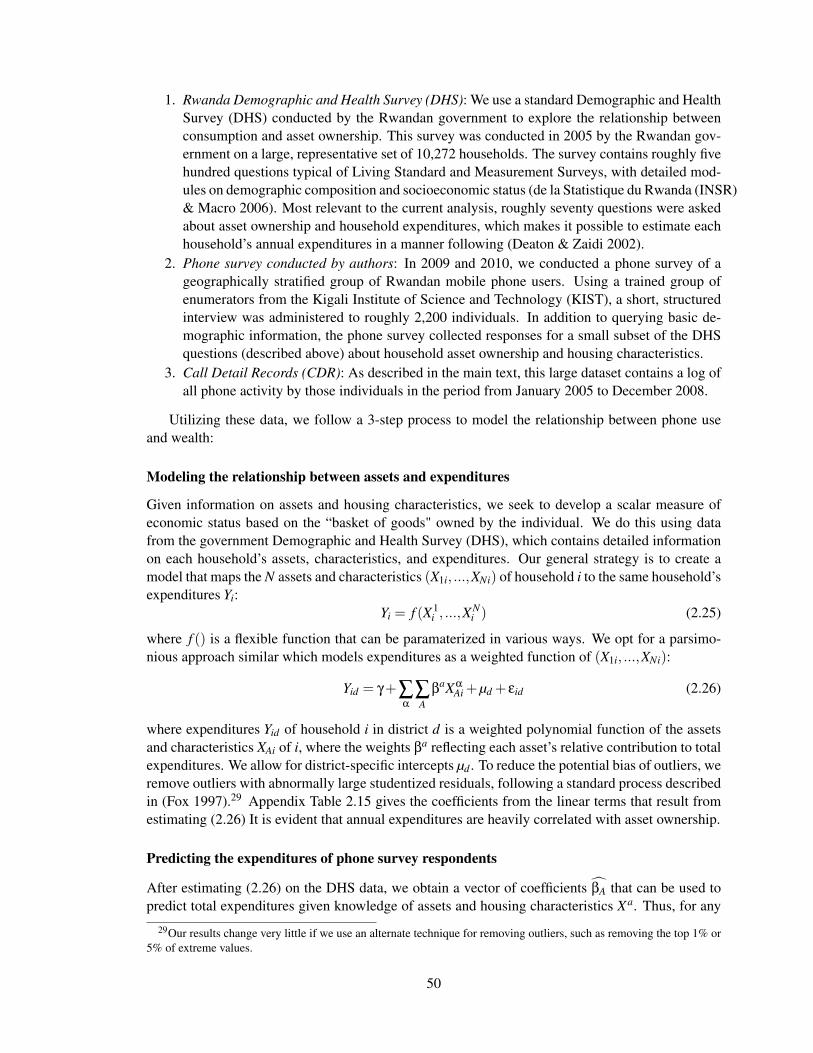
1. Rwanda Demographic and Health Survey (DHS): We use a standard Demographic and HealthSurvey (DHS) conducted by the Rwandan government to explore the relationship betweenconsumption and asset ownership. This survey was conducted in 2005 by the Rwandan gov-ernment on a large, representative set of 10,272 households. The survey contains roughly fivehundred questions typical of Living Standard and Measurement Surveys, with detailed mod-ules on demographic composition and socioeconomic status (de la Statistique du Rwanda (INSR)& Macro 2006). Most relevant to the current analysis, roughly seventy questions were askedabout asset ownership and household expenditures, which makes it possible to estimate eachhousehold’s annual expenditures in a manner following (Deaton & Zaidi 2002).

2. Phone survey conducted by authors: In 2009 and 2010, we conducted a phone survey of ageographically stratified group of Rwandan mobile phone users. Using a trained group ofenumerators from the Kigali Institute of Science and Technology (KIST), a short, structuredinterview was administered to roughly 2,200 individuals. In addition to querying basic de-mographic information, the phone survey collected responses for a small subset of the DHSquestions (described above) about household asset ownership and housing characteristics.

3. Call Detail Records (CDR): As described in the main text, this large dataset contains a log ofall phone activity by those individuals in the period from January 2005 to December 2008.

Utilizing these data, we follow a 3-step process to model the relationship between phone useand wealth:

Modeling the relationship between assets and expenditures

Given information on assets and housing characteristics, we seek to develop a scalar measure ofeconomic status based on the “basket of goods" owned by the individual. We do this using datafrom the government Demographic and Health Survey (DHS), which contains detailed informationon each household’s assets, characteristics, and expenditures. Our general strategy is to create amodel that maps the N assets and characteristics (X1i, ...,XNi) of household i to the same household’sexpenditures Yi:

Yi = f (X1i , ...,X

Ni ) (2.25)

where f () is a flexible function that can be paramaterized in various ways. We opt for a parsimo-nious approach similar which models expenditures as a weighted function of (X1i, ...,XNi):

Yid = γ+∑α

∑A

βaXα

Ai +µd + εid (2.26)

where expenditures Yid of household i in district d is a weighted polynomial function of the assetsand characteristics XAi of i, where the weights βa reflecting each asset’s relative contribution to totalexpenditures. We allow for district-specific intercepts µd . To reduce the potential bias of outliers, weremove outliers with abnormally large studentized residuals, following a standard process describedin (Fox 1997).29 Appendix Table 2.15 gives the coefficients from the linear terms that result fromestimating (2.26) It is evident that annual expenditures are heavily correlated with asset ownership.

Predicting the expenditures of phone survey respondents

After estimating (2.26) on the DHS data, we obtain a vector of coefficients βA that can be used topredict total expenditures given knowledge of assets and housing characteristics Xa. Thus, for any

29Our results change very little if we use an alternate technique for removing outliers, such as removing the top 1% or5% of extreme values.

50

individual in Rwanda, we could in principle predict that individual’s annual expenditures, denotedby Yid , by asking that individual a small number of questions about his household.30 Through ourphone-based surveys, we collect information on the assets and housing characteristics (i.e., the XA)which maximize the predictive power of Equation 2.26. To determine which XA to collect in thephone surveys, we ran feature selection algorithms on the DHS data – in rough terms, this processidentifies the characteristics which will maximize the R2 of g(·).31

Relating call histories to predicted expenditures

Using the above technique, it is possible to obtain the predicted expenditures Yid for each of the in-dividuals contacted in the phone survey. This gives us a total of roughly 2,200 individuals for whomwe have a measure of predicted expenditures and detailed call history information (obtained fromthe mobile operator). For these individuals, it is then possible to directly evaluate the relationshipbetween phone use and economic status:

Yid = g(CDRi) (2.27)

Finding the optimal form of g(·) is an important research topic, but is not our primary focus. Again,we opt for a parsimonious approach and estimate a fixed-effects regression of predicted expenditureson a large number of aggregate statistics of mobile phone use in a manner similar to (2.26). Wecompute a large number of metrics of phone use CDRi. To minimize potential endogeneity of τi jt ,we exclude all data on interpersonal transfers, and instead focus on each subscribers history ofphone calls, text messages, recharge (“top-up") purchases, and a large number of social networkmetrics. Some of the characteristics include:

• Activation date: The date on which the phone first appears in the transaction logs.• Days of activity: The number of different days on which the phone was used.• Net calls: Number of outgoing calls minus the number of incoming calls.• Degree: Number of unique contacts with whom the person communicated (called or received

a call).• Daily degree: Average number of unique people contacted on any given day, conditional on

phone use.• Recharge: Monetary value deposited on SIM card.• In/Out-degree: Number of different people to whom/from whom, calls were made/received.• Clustering: Percentage of first-degree contacts that have contacted each other.• Betweenness: Average shortest path between the user and 50 randomly sampled numbers.• Interpersonal transfers: Total airtime transfers (number sent + number received).• Districts: Number of political districts in which the phone was used. Rwanda has 30 districts.

Appendix Table 2.16 summarizes these metrics for a representative random sample of mobilesubscribers, and Appendix Table 2.17 presents the results from regressing predicted expenditureson twelve different metrics of phone use (polynomial terms excluded). The R2 of 0.21 – whichincreases to 0.39 after including polynomial terms, district fixed effects, and several other metricsof phone use – indicates a strong relationship between expenditures and phone use.

Potential endogeneity and other limitations

The identification strategy used in Section 2.6.2 2.6.2 relies on a proxy for permanent income, xi,to measure the relative socioeconomic status of the population of mobile phone subscribers. In

30In practice, there are some outlandish assumptions that must be made to justify this approximation, but we will deferdiscussion of these and other limitations until the end of the Appendix.

31Full details on the process of feature selection, and the characteristics found to most predictive of annualized expen-ditures, are available from the authors.

51

utilizing the Yid as computed above, one potential concern is that our xi is more a proxy of aggregatephone use or technological sophistication than actual economic wealth. We take three steps tominimize this possibility. First, as noted above, in estimating (2.27) we exclude all metrics relatedto use of the airtime transfer service. Second, we use a highly non-parametric model to estimate(2.27) that includes district fixed effects and second- and third-order polynomial terms. As a result,

there are strong non-monotonicities in (2.27) such that Yid is increasing in some measures of phone

use, decreasing in others, and in general is highly non-linear. This ameliorates the concern that Yidsimply captures aggregate phone use. Finally, we can explicitly control for different measures of

aggregate phone use in our regressions that include Yid .Appendix Table 2.18 presents the results of re-estimating the partial effect of wealth on transfers

received (Table 2.5 in the main text), while additionally controlling for “Recipient Calling Activity,"which is simply the total number of calls made by the recipient in 2007. We assume that this measureis likely to be more directly correlated with the recipient’s general propensity to utilize the phone

than our non-parametric measure of wealth xi =Yid . Comparing the results of Appendix Table

2.18 with Table 2.5, we note that all coefficients have the same sign and statistical significance.In particular, the correlation between recipient wealth and transfers received remains positive andsignificant.32

Apart from the above concern, there are several limitations worth highlighting in the approachwe have taken to estimating wealth from call records. We have glossed over distinctions betweenincome, expenditures, permanent income, and wealth, which are of material consequence in evalu-ating poverty and development (cf. Deaton & Muellbauer 1980). Also problematic is the possibilitythat asset-based proxies for expenditures may provide biased estimates of the expenditures of cer-tain types of individuals. For instance, if a strong correlation is found between television ownershipand assets among the aggregate population, but a small subgroup of the population has a distastefor television, this simple method would systematically underestimate the expenditures of that sub-group. Finally, one particularly troubling assumption we must make is that the relationship betweenassets and expenditures identified with the function f (·) in the 2005 DHS data will remain constantwhen applied to phone survey data collected in 2009 and 2010. This assumption is unjustified for atleast two distinct reasons. First, the data for the two populations was collected using very differentmethodologies, and respondents may respond differently to questions about assets depending onwhether they are asked in person or over the phone. Second, the data was collected in differentyears, and it is possible that the relationship between assets and expenditures would evolve oversuch a long interval. For instance, the strong relationship observed in 2005 between television own-ership and wealth may be weaker in 2010, as electricity becomes more available and used televisionssaturate the market.

In noting these weaknesses and still using Yid as a proxy for xi, we do not mean to imply thatthis method will provide an accurate or unbiased measure of an individual’s wealth. However, wehope that amidst all of the noise there is a decipherable signal that lets us infer the relative wealth ofindividuals in our mobile phone dataset, for whom we only have anonymous records of phone use.

2.8.4 Appendix Tables

32In separate results, available from the authors, we control for other measures of calling activity (such as the sum ofcalls made and received). These alternate specifications produce very similar point estimates and standard errors to thosepresented in Appendix Table 2.18.

52

Table 2.7: Net transfers and Distance(1) (2) (3)

No Fixed Effects Avg. Partial Effects Fixed Effects

Shock (recipient) 4.191** 3.901**

(1.39) (1.31)

Di jt * Shock -0.117* -0.116*

(0.05) (0.05)

Si j * Shock 0.178 0.191

(0.13) (0.12)

Distance (Di jt) -0.013** -0.021***

(0.00) (0.00)

Social Proximity (Si j) 0.050*** 0.050***

(0.00) (0.00)

Day dummies yes yes yes

Fixed effects None None Dyad (directed)

Number of observations 9915422 193256 9915422

Notes: Outcome is τi jt , the total airtime received by i from j on day t. Regressions include observations fromthe period January 4, 2009 through March 3, 2008. Di jt measures the distance between i and j in kilometerson day t, using the locational inference algorithm described in Section 2.5.2. Si j is measured by counting thenumber of phone calls between i and j in the last three months of 2007. All regressions include NearE picenteritand pairwise interaction terms (e.g. Di jt * NearE picenterit , Di jt*DayO f Quaket ); these coefficients are omittedfor clarity. Standard errors, clustered by district, reported in parentheses. *** p<0.001, ** p<0.01, * p<0.05,+ p<0.10.

53

Table 2.8: Sensitivity of estimation to function form assumptions

(1) (2) (3) (4)Pooled OLS OLS w/Controls Region FE Region & Day FE

Earthquake Shock 1793.639*** 2819.503*** 2787.305*** 2710.861***(313.08) (121.33) (136.18) (183.53)

DayO f Quake -748.548** -1375.294*** -1287.145***(212.87) (111.76) (119.77)

NearE picenterit -2262.728*** -510.751***(577.57) (73.57)

Total call volume 0.074*** 0.064*** 0.103***(0.00) (0.01) (0.01)

Outgoing transfers 0.677*** 0.637*** 0.527***(0.03) (0.03) (0.04)

Tower Fixed Effects No No Yes YesDate Fixed Effects No No No YesR2 0.008 0.702 0.729 0.753N 171414 74895 74895 74895

Notes: Outcome is the total amount transferred into a tower on a single day. NearE picenter definedas those towers within 20 miles of the earthquake epicenter. Columns 2-4 include controls foroverall network activity at the tower-day level. Column 3 includes tower-level fixed effects. Column4 includes daily fixed effects. Estimates made using data from October 1, 2006 through July 1, 2008.Heteroskedasticity-robust SE’s in parentheses (clustered at district level). * p<0.05, ** p<0.01, ***p<0.001.

54

Table 2.9: Lagged effects of the earthquake on transfers and calls received.

(1) (2) (3)Transfers Received Calls Received Int’l Calls Received

Shock 13512.649*** 14208.656*** 142.584*(1335.51) (3753.46) (56.71)

shock_lag1 -917.294 4594.386*** 126.538(1330.88) (499.87) (76.47)

shock_lag2 1540.204 1639.237 62.719(2796.36) (1026.90) (49.83)

shock_lag3 830.593 1297.175*** 47.690(3157.92) (295.21) (33.18)

shock_lag4 -189.597 552.066* -28.472(1518.35) (208.00) (17.58)

shock_lag5 -40.867 1070.376*** -66.248*(3028.17) (229.54) (29.46)

shock_lag6 -2648.816 927.869** -95.259(3138.61) (303.77) (58.89)

shock_lag7 -335.684 1468.774** -86.875(849.38) (420.29) (46.27)

shock_lead1 810.813 228.141 34.601(1732.01) (316.09) (25.81)

shock_lead2 1341.489 218.922 40.632(1124.93) (387.07) (44.32)

shock_lead3 -2460.249 -72.909 -24.811(2003.26) (201.42) (59.38)

Total call volume 0.010(0.01)

Outgoing transfers 0.876***(0.02)

Outgoing calls 0.969***(0.00)

Outgoing int’l calls 0.959***(0.02)

Constant 155.928 2069.706 1417.339***

R2 0.984 1.000 0.943N 16808 18840 18840

Notes: Outcome specified in column heading. All specifications include dailyand district fixed effects. Heteroskedasticity-robust standard errors in parenthesis(clustered at district level).

55

Table 2.10: Placebo Tests - Region

(1) (2) (3) (4) (5)1 week early 1 month early 2 months early 1 month late 2 months late

placebo -55.046 -883.510 476.872 422.916 -165.949(333.48) (671.79) (1098.90) (424.18) (356.80)

placebo_lag1 -381.418 -53.947 -618.709 2003.713 11.852(618.73) (217.97) (612.11) (1128.16) (247.78)

placebo_lag2 -984.936 -1168.092∗ -26.755 50.986 1436.589∗∗∗

(541.80) (510.72) (458.54) (925.05) (302.94)placebo_lag3 -961.343 130.801 -1566.041 -2797.677∗∗∗ -254.537

(603.55) (484.92) (1163.88) (722.97) (333.08)placebo_lag4 -764.067 -828.406∗ -535.389 -542.332 662.051

(465.33) (349.95) (895.21) (609.62) (401.94)placebo_lag5 818.791 -1152.675 -388.534 396.936 83.309

(1436.49) (747.69) (1208.20) (548.55) (206.67)placebo_lag6 1032.607 -671.954∗∗ -789.253 -759.333 1191.760

(880.44) (182.22) (529.11) (1680.09) (586.25)placebo_lag7 252.983 88.647 268.176 225.380 835.777∗∗

(257.85) (838.98) (697.38) (1449.35) (250.26)calls_gross 0.103∗∗∗ 0.103∗∗∗ 0.103∗∗∗ 0.103∗∗∗ 0.103∗∗∗

(0.01) (0.01) (0.01) (0.01) (0.01)transfer_val_out 0.529∗∗∗ 0.529∗∗∗ 0.529∗∗∗ 0.529∗∗∗ 0.529∗∗∗

(0.03) (0.03) (0.03) (0.03) (0.03)_cons 737.229 737.553 737.288 737.174 736.841

r2 0.754 0.754 0.754 0.754 0.754rmse 4025.238 4025.264 4025.233 4025.195 4025.252N 74300.000 74300.000 74300.000 74300.000 74300.000

Outcome: Value of incoming airtime sent to people in district (in RWF; US$1=550RWF). Heteroskedasticity-robust SE’s

in parentheses (clustered at district level).

56

Table 2.11: Effect of flood on transfers(1) (2) (3) (4)

Pooled OLS OLS controls tower FE tower/Time FE

Flood Shock 1456.901 933.040∗∗ 1029.241∗∗ 1068.659∗∗

(770.84) (316.98) (329.36) (375.45)DaysO f Floodt 774.798∗∗∗ 952.838∗∗∗ 981.247∗∗∗

(166.92) (230.79) (206.75)NearE picenterit 263.474 237.740∗

(919.80) (88.55)Total calls 0.075∗∗∗ 0.065∗∗∗ 0.103∗∗∗

(0.00) (0.01) (0.01)Outgoing transfers 0.678∗∗∗ 0.637∗∗∗ 0.527∗∗∗

(0.03) (0.03) (0.04)

R2 0.000 0.702 0.729 0.753N 171414 74895 74895 74895

“In flood region" defined as towers in the two districts affected by the flood. “Days of flood" are

9/12/07 - 9/18/07.

57

Table 2.12: Net transfers and wealth (Robustness to sender FE)

Earthquake Shock 9.727*(4.36)

Recipient Wealth xi * Shock 5.702***(1.31)

Sender Wealth (x j) * Shock 15.299(13.93)

Social Proximity Si j * Shock 0.102(0.07)

Recipient Wealth (xi) 0.847***(0.17)

Social Proximity (Si j) 0.069***(0.00)

Day dummies YesFixed effects Sender jNumber of observations 10032721

Notes: Outcome is τi jt , the total airtime received by i from j on day t. Re-gressions include observations from the period January 4, 2009 through March3, 2008. Wealth proxies xi and x j are computed using equations (2.14) and(2.15), as described in the text. Si j is measured by counting the number ofphone calls between i and j in the last three months of 2007. All regressions in-clude NearE picenterit and pairwise interaction terms (e.g. xi * NearE picenterit ,xi*DayO f Quaket ); these coefficients are omitted for clarity. Standard errors,clustered by district, reported in parentheses. *** p<0.001, ** p<0.01, *p<0.05, + p<0.10.

58

Table 2.13: Network Flow as Social Proximity

(1) (2) (3)No Fixed Effects Avg. Partial Effects Fixed Effects

Shock (recipient) 8.935* 8.480+(4.33) (4.16)

Recipient Wealth xi * Shock 6.791*** 6.806***(0.75) (0.95)

Sender Wealth x j * Shock 16.501 15.766(14.74) (13.66)

Network Flow Si j * Shock -0.918 -0.846(0.62) (0.51)

Recipient Wealth (xi) 1.146*** 1.266***(0.17) (0.10)

Sender Wealth (x j) 1.915*** 1.892***(0.12) (0.14)

Network Flow (Si j) 0.048 0.054***(0.03) (0.02)

Day dummies Yes Yes YesFixed effects None None Dyad (directed)Number of observations 10032721 10032721 10032721

Notes: Outcome is τi jt , i.e. airtime received by i from j on day t. xi and x j are estimated using equations(2.14) and (2.15), described in text. Si j measures the number of distinct paths between i and j, where a pathis defined by the call graph. All regressions include NearE picenteri and pairwise interaction terms (e.g. xi *NearE picenteri, xi*DayO f Quaket ), but results are omitted for clarity. Standard errors, clustered by district,reported in parentheses. *** p<0.01, ** p<0.05, * p<0.1.

59

Table 2.14: Robustness of dyadic results

(1) (2) (3) (4) (5)

Clustering j’s District j’s Tower j Day t Unique senders

Earthquake Shock 9.794** 9.792*** 9.892*** 9.892*** 7.591*

(4.33) (3.51) (3.77) (0.31) (4.63)

xi * Shock 5.763*** 5.770** 6.011* 6.011*** 0.145

(1.26) (2.89) (3.39) (0.40) (0.22)

x j * Shock 14.903 14.833 14.684 14.684*** 8.929

(13.33) (12.12) (11.86) (0.97) (7.23)

Si j * Shock 0.110 0.111 0.110 0.110*** 0.260

(0.07) (0.12) (0.15) (0.01) (0.21)

Day fixed effects Yes Yes Yes Yes Yes

Fixed effects Dyad Dyad Dyad Dyad Dyad

N 10,032,721 10,032,721 10,251,136 10,251,136 4,430,160

Notes: Specification is identical to that used to produce column (3) of Table 2.5, with standarderrors clustered according to column labels. Column (5) clusters by recipient, but restricts sampleto allow only one recipient per sender. In cases were a single sender sends to multiple recipients,one recipient is chosen at random and the others are dropped from the analysis. Slightly fewerobservations are contained in (1) and (2) because the tower closest to j is unknown for certain days.* p <0.05, ** p<0.01, *** p<0.001.

Table 2.15: Regression of Expenditures on Asset Ownership

Outcome log(Expenditures) Expenditures

βa (S.E.) βa (S.E.)

Radio 0.18 (0.02) 40090 (13007)

Television 1.14 (0.01) 2130434 (44048)

Bed 0.24 (0.04) 187061 (8266)

Table 0.13 (0.01) 57601 (9109)

Car/Truck 0.24 (0.01) 1695284 (57718)

Motorcycle 0.65 (0.04) 8229976 (197091)

Bicycle 0.22 (0.11) 138186 (20359)

HH Size 0.09 (0.02) 56168 (3198)

R2 0.62 0.75

N 6900 6900

Notes: Standard errors reported in parentheses.

60

Table 2.16: Summary statistics of phone use as computed from transaction logs

AveragePanel A: Domestic and International CallsActivation date 1/12/08Days of activity 770.3Avg. call length 31.7Calls per day 6.25Net calls per day (out-in) 0.087Int’l calls per day 0.084Net int’l calls (out-in) -0.014Panel B: Social Network StructureDegree 734In-degree 488.2Out-degree 433Daily degree 3.78Net daily degree (out-in) 0.00027Clustering 0.063Betweenness 2.72Panel C: Other BehaviorsCredit used per day 163.5Max. recharge value 2756.3Avg. districts per day 1.36Avg. districts contacted 1.21N 901

Notes: Mean values reported, weighted by sampling strata to

produce averages representative of entire phone population.

61

Table 2.17: Regression of predicted expenditures on phone use

Coefficient (S. E.)

Duration (outgoing) -0.75 (2.55)Duration (incoming) 7.66∗∗∗ (2.01)Degree -1038.70∗ (439.98)Int’l duration (out) -17.60 (10.07)Int’l duration (in) -10.63 (7.78)Int’l degree 10534.70∗∗∗ (3883.26)Districts called 129304.11∗∗ (42014.00)Districts received -103121.07∗∗ (36356.38)Unique towers 2918.14 (3600.54)Months 11916.91 (9027.69)Avg. recharge denomination 602.87 (461.13)Daily recharge 716.18 (794.48)

N 671R2 0.21

Outcome is predicted expenditures Yid , in RWF. Standard errors inparentheses. ∗ significant at p < .05; ∗∗p < .01;∗∗∗p < .001.

62

Table 2.18: Robustness check: net transfers and wealth(1) (2) (3)

No Fixed Effects Avg. Partial Effects Fixed Effects

Earthquake Shock 9.803* 9.364*(4.67) (4.38)

Recipient Wealth xi * Shock 8.764** 8.616**(2.51) (2.43)

Sender Wealth x j * Shock 15.745 14.913(14.40) (13.38)

Social Proximity Si j * Shock 0.118+ 0.127+

(0.07) (0.06)Recipient Calling Activity * Shock -0.004+ -0.003*

(0.00) (0.00)Recipient Wealth (xi) 1.382*** 1.416***

(0.21) (0.12)Sender Wealth (x j) 1.624*** 1.622***

(0.11) (0.13)Social Proximity (Si j) 0.043*** 0.043***

(0.00) (0.00)Recipient Calling Activity -0.001*** -0.001***

(0.00) (0.00)

Day dummies Yes Yes YesFixed effects None None Dyad (directed)Number of observations 9984468 174657 9984468

Notes: Outcome is τi jt , i.e. airtime received by i from j on day t. xi and x j are estimated using equations (2.14) and(2.15), described in text. Si j measures the number of phone calls between i and j in the three months prior to theearthquake. “Recipient Calling Activity" counts the total number of calls made by i in 2007. All regressions includeNearE picenteri and pairwise interaction terms (e.g. xi * NearE picenteri, xi*DayO f Quaket ), but results are omittedfor clarity. Standard errors, clustered by district, reported in parentheses. *** p<0.001, ** p<0.01, * p<0.05, +p<0.10.

63

64

CHAPTER 3INFERRING PATTERNS OF INTERNAL

MIGRATION FROM MOBILE PHONE

CALL RECORDS

3.1 Abstract

Understanding the causes and effects of internal migration is critical to the effective design andimplementation of policies that promote human development. However, a major impediment todeepening this understanding is the lack of reliable data on the movement of individuals within acountry. Government censuses and household surveys, from which most migration statistics arederived, are difficult to coordinate and costly to implement, and typically do not capture the patternsof temporary and circular migration that are prevalent in developing economies. In this chapter, wedescribe how new information and communications technologies, and mobile phones in particular,can provide a new source of data on internal migration. As these technologies quickly proliferatethroughout the developing world, billions of individuals are now carrying devices from which it ispossible to reconstruct detailed trajectories through time and space. Using Rwanda as a case study,we demonstrate how such data can be used in practice. We develop and formalize the concept of in-ferred mobility, and compute this and other metrics on a large dataset containing the phone recordsof 1.5 million Rwandans over four years. Our empirical results corroborate the findings of a recentgovernment survey that notes relatively low levels of permanent migration in Rwanda. However,our analysis reveals more subtle patterns that were not detected in the government survey. Namely,we observe high levels of temporary and circular migration, and note significant heterogeneity inmobility within the Rwandan population. Our goals are thus twofold. First, we intend to providea new quantitative perspective on certain patterns of internal migration in Rwanda that are unob-servable using standard survey techniques. Second, we seek to contribute to the broader literatureby illustrating how new forms of information and communication technology can be used to betterunderstand the behavior of individuals in developing countries.1

1The material in this chapter is based on material originally published in 2012. See: Blumenstock (2012).

65

3.2 Introduction

A country’s overall development trajectory is intimately connected to the way in which its inhab-itants move about. Internal migration, defined as the temporary or permanent relocation of in-dividuals within a country, can have a profound impact on regional labor markets (Borjas 2006,Todaro 1980, Greenwood 1985),2 affect levels of urban and rural inequality (Lucas, Rosenzweig &Stark 1997), and provide vectors for disease transmission (Busenberg & Travis 1983), to name justa few examples. As a result, many governments in developing countries have gone to great lengthsto regulate the movement of populations, instituting sometimes draconian, and often futile, policiesto inhibit migration (Shrestha 1987, Simmons 1979).

As policymakers and academics gain more insight into the consequences of migration, so toohave researchers grappled with understanding the causes of migration (Borjas 1999, Lucas et al.1997). While the canonical model posits that individuals migrate primarily to earn higher wages(Todaro 1969), more recent work has shown that the decision to migrate is far more complex.For instance, Munshi (2003) used longitudinal data from Mexico to show that the migrant’s socialnetwork in the destination location had a large impact on his later success and subsequent migrationdecisions. Using cross-sectional data, a number of other studies have shown that migrants and non-migrants tend to come from different socioeconomic classes, different age groups, and differentgenders. More generally, it also appears that certain types of individuals are more likely to be moremobile on a daily basis, irrespective of more permanent migratory behavior (Frias-Martinez, Virseda& Frias-Martinez 2010, Maheswaran, Pearson, Jordan & Black 2006).

Despite the burgeoning literature on both the causes and effects of migration, the empiricalmethods used to measure and evaluate migration - and internal migration in particular - remainquite rudimentary. Over the past few decades, a number of prominent academics have pointed to theinadequacy of reliable data as a major constraint to research on migration (Banerjee & Duflo 2007,McKenzie & Rapoport 2007, Lucas et al. 1997, Bilsborrow 1997, Massey 1990). This constraint isexacerbated in developing countries, where limited infrastructure is in place to coordinate migration-specific surveys.

In this paper, we discuss how new information and communication technologies (ICTs), andhow mobile phones in particular, can provide researchers with new insight into patterns of migrationand human mobility.3 After discussing in greater depth the limitations of the current data (Section3.3) and the advantages that ICT-generated data have over more traditional data (Section 3.4), wedemonstrate the proposed empirical analysis using Rwanda as a case study (Section 3.5). We de-velop a new quantitative measure of inferred mobility that we use to compute rates of temporaryand circular migration from call records that we obtained from the Rwandan telecommunicationsoperator. Our results indicate that although rates of permanent internal migration are moderate, therates of temporary and circular migration are much higher. We finish with a discussion of the im-plications of our findings to researchers interested in social development, and of the limitations ofour methodology, with a particular focus on the ethical concerns arising in the use of ICTs to trackmovement (Section 3.6). Section 3.7 concludes.

2We focus our attention primarily on the effect of internal migration. For surveys of the much larger literature on thelabor market effects of international migration, see Friedberg & Hunt (1995) and Borjas (1999)

3A vibrant literature is being developed to describe the ways in which ICTs can have a positive impact on the livesof people and their communities, and on their social development (Aker 2008, Jensen 2007, Qureshi 2009, Blumenstocket al. 2011). While this paper is intimately related to that literature, the goal is different. Our intent, rather, is to emphasizehow ICTs can help researchers and policymakers better measure and evaluate processes of development, rather than assessthe causal impact of the interventions themselves (be they ICT-based or not).

66

3.3 The challenge of measuring internal migration in developing coun-tries

Internal migration, both permanent and seasonal, is extremely common in most developing coun-tries. For instance, Banerjee & Duflo (2007) note that 60 percent of the poorest households inRajasthan, the largest state in India, report that someone from their family left the home for part ofthe year to obtain work. Aker, Clemens & Ksoll (2011) observe that over 45 percent of householdsin Niger have at least one seasonal migrant, and Skeldon (1986) notes that roughly 30 percent ofIndians reported permanently living in a place other than the place of survey enumeration. Thoughmuch of the policy debate surrounding migration has focused on urbanization and the permanentresettlement of citizens from rural areas to cities, empirical evidence suggests that rates of rural-to-rural migration may be much higher (Banerjee & Duflo 2007, Cohen & Dupas 2007).

Unfortunately, much of the empirical quantitative research has been hindered by a lack of reli-able statistics on migration. Indeed, most developing country governments track only a handful ofmigration-related statistics (Lucas et al. 1997). Moreover, the statistics that do exist are potentiallyquite misleading. Part of the difficulty stems from the fact that migrants, by definition, leave oneplace and resettle in another, complicating the prospect of longitudinal interviews with migrants andadding bias to metrics that do not account for such movement. In discussing a long-term trackingstudy of migrants in Tanzania, Beegle, De Weerdt & Dercon (2011) summarized the problem asfollows:

The costs and difficulties of resurveying means that attrition may be relatively high for[migrants] and may also result in the loss of some of the most relevant households forthe study of this process... Had we not tracked and interviewed people who moved outof the community, a practice that is not carried out in many panel surveys, we wouldhave seriously underestimated the extent to which poverty decreased... we would havereported poverty reduction at about half its true value.(p.2)

In practice, migration-specific survey modules such as the one employed by Beegle et al. (2011)require considerable time and resources to deploy, and are prohibitively expensive for most re-searchers and government agencies. This is especially true in developing countries, which oftenlack the substantial administrative infrastructure required to develop an instrument, train enumera-tors, analyze the data, and otherwise coordinate (and fund) a large survey. Thus, the vast majorityof research on migration relies at some level on aggregate population statistics such as censuses andpopulation registers.

These aggregate statistics may be appropriate for certain lines of inquiry - for instance, they candescribe rough patterns of international migration, and of net urban-rural migration, two phenomenathat have been at the center of the policy debate on migration. However, the typical governmentcensus occurs only once every ten years, and does not record fine-grained demographic shifts inthe population. Censuses are also notoriously biased toward documented citizens, often failingto capture the extent and significance of undocumented or international migrants (Massey 1990).More detailed surveys, when available, are often ad hoc and not standardized. For instance, arecent survey of worldwide statistics on internal migration found that of the 38 African countriesstudied, no more than 10 had a common definition of the requisite time interval required to qualifysomeone as a migrant (Bell & Muhidin 2009). This inconsistency is not unique to Africa. Carletto& de Brauw (2007) note that only one country of the 89 they surveyed was compliant with theUN Recommendations on Statistics of International Migration. To give one final example, Lucaset al. (1997), in his review of the migration literature, attempted to separate urban city growth into

67

the components due to natural population growth and the component due to actual rural-to-urbanmigration. However, he found that only 29 countries worldwide had census data with sufficientlydetailed questions to perform this decomposition.4

Of particular relevance to those interested in developing countries, standard censuses and popu-lation registers often fail to track patterns of temporary and seasonal migration. The difficulty arisesbecause a seasonal migrant, who leaves his place of residence but returns every year, would notbe noted in a standard survey or census, since the place of residence and of enumeration may notdiffer. Yet, these forms of migrations are extremely common in developing countries, and in Africaand Asia in particular (Nelson 1976). Moreover, these distinctions are not without consequence. AsNelson (1976) observes, “people who regard themselves as sojourners in the city will seek differentkinds of housing, demand fewer amenities and services, behave differently with respect to makingfriends and joining organizations, use accumulated savings for different purposes, and respond todifferent political issues and candidates than will people committed to the city as their permanenthome.” (p. 721) We take these shortcomings of the migration data as motivation for the current re-search, which seeks to explore alternative mechanisms for gathering and analyzing data on internalmigration.

3.4 How ICTs can provide better measures of migration and mobility

With the proliferation of mobile phones and other information and communication technologies(ICTs) in developing countries, billions of individuals now carry devices that can record fine-grainedinformation on the trajectories of those persons through time and space. The combined data fromthese individuals thus forms a massive data repository on patterns of migration and mobility. More-over, many of these individuals are precisely those whom statistical agencies have found so difficultto survey, such as undocumented citizens and those living in extremely remote areas. There are,of course, significant privacy concerns that arise when any agency or organization keeps detailedrecords of individual’s location. This is particularly true with data that is unobtrusively collected,and for which it is often impractical to obtain the informed consent of the subjects under study.Ethical concerns such as these are discussed in greater detail in Section 3.6.2.

In recent years, a small but vibrant literature has developed around the ways in which ICTscan be used to better understand patterns of human movement.5 To date, such research generallyemploys two distinct sources of data. The first involves custom ICT-based deployments, whereresearchers give subjects devices or software that monitors movement and behavior. In an earlyexample of such research, Eagle & Pentland (2006) gave 100 volunteer U.S. students and facultysmartphones equipped with special software that continuously tracked the subjects’ locations andphone-based interactions. They found that, given information about a subject’s movements duringthe first half of a day, they could then predict the subject’s whereabouts for the rest of the day withroughly 80 percent accuracy. Using similar software given to 200 mobile phone users, Gonzalezet al. (2008) showed that despite the diversity of individual travel patterns, most humans followsimple and reproducible patterns.

The second approach to measuring mobility with ICTs, and the one which we utilize in theempirical analysis that follows, employs the data inadvertently generated in the everyday use of

4Bilsborrow (1997) provides an excellent overview of the strengths and weaknesses of the different sources of migra-tion data.

5A very closely related body of research addresses the ways in which ICTs can be used to better understand otheraspects of human behavior beyond mobility and migration, including the spread of innovations and products (Szabo &Barabasi 2006), and patterns of economic growth (Eagle, Macy & Claxton 2010). See Kwok (2009) and Hazas, Scott &Krumm (2004) for brief overviews of this literature.

68

technology, and requires no special device or software to be given to the subject. For the study ofpopulations in developing countries, the mobile phone is the obvious choice, with over five billionsubscribers worldwide (77 percent of the world population), and roughly 68 percent penetration inthe developing world.6 More sophisticated GPS-enabled devices continuously record the exact geo-coordinates of the subscriber, but even the most rudimentary mobile phone can be roughly locatedin space based on the cell towers which are used to route calls and data sent between the deviceand the network. Based on the sequence of towers which the individual uses, it is possible to laterreconstruct the approximate path which that person traveled.

In urban areas, where towers are quite dense, the geographic precision of tower-based locationalinference can be quite precise, though the resolution decreases in rural areas, where towers aresparser. To provide a more concrete example, Figure 3.1 depicts the approximate location of allmobile towers in Rwanda circa 2008. Each dot represents a single tower, and the straight linesdemarcate the Dirichlet cells corresponding to the approximate coverage region of each tower. Theurban capital of Kigali is evident in the dense cluster of cells in the center of the figure. In Figure3.2, we superimpose on the Voronoi diagram the trajectory of two mobile subscribers over a four-year period from early 2005 through late 2009. For each month in that period, we extrapolatethe approximate location of the individual (based on the individual’s center of gravity, a conceptthat is defined formally in the following section), and plot that point on the Rwandan map. Earlylocations are colored dark red, while later locations are yellow; subsequent month-locations areconnected with a solid line. The first figure depicts a typical individual living in the urban capital,who remains in roughly the same location over the four-year period. The second figure shows anindividual who is seen to migrate twice, once in mid-2006 and again in early 2008.

Using data of this nature, it is possible to measure the patterns of mobility and migration at alevel of precision and temporal resolution that would be impossible using standard survey method-ologies. To date, however, we are aware of only two studies have utilized individual movementlogs to analyze patterns of mobility. In the first, Eagle et al. (2009) compared usage trends be-tween urban and rural citizens of a small developing country, and showed that individuals in ruralareas travel significantly more per month than individuals in the cities, noting this “could be due tothe small potential distances that can be traveled within the capital and the much larger distanceswithin rural areas” (p.146). Using similar data from the “main city of a Latin-American country,”(Frias-Martinez, Virseda & Frias-Martinez 2010) showed that people from areas of higher socio-economic status tend to be more physically mobile than people from poorer parts of the same city.Though both of these studies are evocative examples of the richness of the data, neither focuses onthe phenomenon of internal migration, and both stop short of providing links to the broader devel-opment discourse. In the next section, we expand upon the work of these researchers, using similardata from Rwanda to very precisely quantify different aspects of internal migration in the country.When possible, we compare our results to official statistics from population censuses and householdsurveys.

3.5 Case Study: Measuring internal migration and mobility in Rwanda

In Rwanda, as in much of sub-Saharan Africa, rates of both internal and international migrationare quite high. The upheaval surrounding the 1994 genocide created a massive refugee crisis thatleft almost 100,000 children orphaned, and dramatically altered the demographic composition of

6http://www.itu.int/ITU-D/ict/statistics/at_glance/KeyTelecom.html, Accessed July 2011. It shouldbe noted, however, that mobile penetration in Africa is the lowest worldwide at 41 percent, and that in certain countriesthe uptake is much lower.

69

Figure 3.1: Map of Rwandan cell phone towers, January 2008. The median area covered by eachtower is roughly 70km2.

70

Figure 3.2: Movement of two different individuals in Rwanda over four years. Each vertex repre-sents that individual’s centre of gravity for a single month, with subsequent months connected byedges. Early months are coloured dark red, with later months appearing orange/yellow. Approxi-mate monthly locations are inferred from the individuals’ history of phone calls using a proceduredescribed in section 3.5.

71

the population. However, the country has been relatively stable for the last decade, and duringthe period of time upon which we focus (2005-2009), anecdotal evidence suggests that patterns ofmigration appear to be comparable to those of neighboring countries (Nkamleu & Fox 2006). Suchbroad generalizations notwithstanding, the actual quantitative evidence on migration in Rwanda,and in particular of the internal migration of Rwandans, is extraordinarily limited. In fact, the onlyrelevant data we are aware of comes from a pair of surveys conducted by the Rwandan governmentin 2006 and 2009. The Comprehensive Food Security and Vulnerability Assessment & NutritionSurvey (CFSVANS), which was conducted on a sample of 5,400 households, asked a small numberof questions about temporary and seasonal migration (de la Statistique du Rwanda (INSR) & Macro2006). Based on these data, the statistical agency reports that 12 percent of the households hadat least one member who moved or migrated during the 3-month period prior to the survey, with11 percent migrating within Rwanda. Numbers are similar in nearby Kenya, with Owen, Brey &Oucho (2008) reporting that 8 percent of individuals aged 15 and older had moved to a new districtin the year before the census. In neighboring Uganda, data from the 2002 census suggests that 12.8percent of Ugandans live in a region other than the one in which they were born, with 5.5 percenthaving migrated in the five years prior to the survey (Ugandan Bureau of Statistics, 2002).

While these numbers provide a useful baseline for understanding internal migration in Rwanda,there are many fundamental questions that remain unanswered. For instance, what would the mi-gration rate be if it were measured at a different time of year? How long do individuals stay in thedestination location, and what percent of migrants eventually return to the place of origin? How dothese numbers compare with more sophisticated mobility-related metrics such as migration inten-sity, the radius of gyration, and the index of net velocity? In the following sections, we demonstratehow mobile phone records, as provided by the national operator, can be used to answer questionssuch as these.

3.5.1 Data

The data we employ in the empirical analysis come from two distinct sources. In the first place,we obtained from Rwanda’s primary telecommunications operator an exhaustive log of all phone-based activity that occurred from the beginning of 2005 through the end of 2008. For each mobilephone user that was active during that period, we have a time-stamped record of every call that theindividual made or received. Further, for each phone-based transaction that was routed through acell phone tower (such as a phone call or text-message), we know the closest tower to the subscriberat the time of the transaction. This allows us to approximately infer the location and trajectory ofroughly 1.5 million mobile subscribers over time and space, in a manner depicted in Figure 3.2.7

However, it is important to note that we only have an intermittent signal of the individual’s location.When the person goes for long periods of time without using his phone, he is effectively “off theradar” and his location is unknown. We will deal with the empirical and analytical implications ofthis intermittency in later subsections.

For the purposes of our empirical analysis, a limitation of the data we employ is that all ofthe records are entirely anonymous and contain no identifying or demographic information on anyof the subscribers. Since we are interested in disaggregating patterns of mobility by demographictype, we have supplemented the anonymous dataset with data gathered during a large-scale phonesurvey that we conducted in Rwanda in 2009 and 2010. For this survey, we obtained the mobile

7During the window of time we examine, the operator we focus on maintained over 90% market share of the mo-bile market. The company’s primary competitor did not gain traction in the market until the end of 2008, and onlymore recently has the market become competitive. The number of landlines in Rwanda is insignificant (roughly 0.25%penetration).

72

phone numbers of a limited number of mobile subscribers and called these individuals to request ashort, structured interview. To help preserve the confidentiality of the respondent we did not collectidentifying information such as the subscriber’s name or address. In total, and with the help of anexcellent group of enumerators from the Kigali Institute of Science and Technology, we completed901 interviews on a geographically stratified sample of the population of mobile phone users.

Thus, for the 901 individuals surveyed we know his or her basic demographic information, aswell as the rough pattern of movement over a 4-year period. For the remaining 1.5 million individ-uals who were not contacted in the phone survey, we have the movement histories but no associateddemographic information. In interpreting the empirical analysis that follows, it is important to notethat, as shown by Blumenstock & Eagle (2012), mobile phone subscribers in this region are differ-ent from non-subscribers - namely, they tend to be wealthier, older, better (formally) educated, andare more likely to be male. As mobile phone penetration approaches 100 percent, this distinctionwill gradually disappear. However, for the population we analyze, it is important to keep in mindthat the external validity of our results applies to mobile phone users in Rwanda, which during theperiod of time under analysis represented between 3 percent (in 2005) and 24 percent (in 2009) ofthe population. Since mobility is generally positively correlated with socioeconomic status (Frias-Martinez, Virseda & Frias-Martinez 2010), we would expect the mobility of the at-large populationto be lower.

3.5.2 Methods

Using the data described above, we compute and analyze a number of different metrics related tothe migration and mobility patterns of phone owners in Rwanda. Since our data comes from asingle country, we focus on internal migration, and the pattern of movement within the country. Wecompute the following statistics based on the mobile phone transaction history:

Number of cell towers used: As a very crude proxy for the movement of the individual, wesimply count the number of unique towers used by the individual during the specified interval oftime. Maximum distance traveled: This is the maximum distance between the set of towers usedby the individual over the interval under study. Radius of gyration (ROG): While the precedingmeasures are quite simple, both have severe limitations, for instance that the number of towers usedwill be much higher for an individual living in an area with many towers, and the maximum distancetraveled will be higher for an individual who uses his phone more often. Thus, we additionallycompute a third metric that is more robust to intermittency and which accounts for the distancebetween towers. As discussed in greater depth by Gonzalez et al. (2008) and Song, Qu, Blumm &Barabasi (2010), the radius of gyration (ROG) is a concept borrowed from Physics which measureshow far an object travels from its center of gravity. In the case of humans, the radius of gyrationroughly measures the typical range of a user in space. A person’s center of gravity is the weightedaverage of all of the points from which the individual makes or receives a call, where the weight isdetermined by the number of times the individual calls from each location. Formally, we denote anarbitrary point in space (within Rwanda) by the vector r. Then, if an individual i makes Ni calls fromlocations (ri1, ...,riNi), that individual’s center of gravity is the vector COGi = (1/Ni)∑

Nit=1 rit . The

radius of gyration is then the root mean square distance of all of the other locations the individualvisits from his center of gravity:

ROGi =

√1Ni

Ni

∑t=1

(rit −COGi)2 (3.1)

While other measures of mobility exist, we selected these three because they are relativelysimple and are among the most commonly employed in the literature. Moreover, many of the

73

different mobility metrics are highly correlated, and we expect most findings to be robust to otherdefinitions of mobility. Inferred migration: While the mobility metrics are relatively objective tocompute, the measurement of migration is less clear cut. As noted earlier, many countries usevarying definitions of a “migrant" in reporting aggregate levels of migration. We define a newmeasure of inferred migration which we use to infer from an individual’s call records whether ornot he or she migrated in a given month. We employ a fairly flexible formulation which defines amigration as occurring at month m if the individual remained in one location for a fixed number of β

months prior to m, and was also stationary for β months after and including m, but that the locationspre- and post-m were different. We call two locations r1 and r2 the same if the distance betweenthem is less than the individual’s radius of gyration times a constant δ. Formally, we denote i’s centerof gravity in month t by COGit ; an inferred migration Mim occurs in month m if the following threeinequalities hold:8

|COGim−COGi(m−1)|>δ∗ROGi (3.2)

|COGi(m−s)−COGi(m−s−1)|<δ

β

β

∑t=1

ROGi(m− t)∀s ∈ [1, ...,β] (3.3)

|COGi(m+s)−COGi(ms−1)|<δ

β

β−1

∑t=0

ROGi(m+ t)∀s ∈ [1, ...,β] (3.4)

The intuition behind the definition of migration is that it accounts for the fact that, in the courseof everyday events, different individuals travel different distances (their radii of gyration). Theparameters α and β allow for a flexible definition of migrant, for instance to account for the dif-ference between a short-term and long-term migrant, and will be discussed in greater detail below.Finally, since we are interested in identifying changes in the individual’s place of residence, ratherthan where they spend their work-days, we restrict our analysis to those phone-based transactionsthat occur between 7pm and 7am. However, this last restriction proves to be immaterial, and ourquantitative results change very little if we include transactions occurring between 7am and 7pm.

3.5.3 Empirical Results

Population aggregates

We begin by computing base rates of internal migration from the mobile phone data for the represen-tative sample of 901 mobile phone users. Unless noted otherwise, we denote by X the populationaverage of X across all n individuals sampled, in other words X = (1/n)∑

nj=0 X j. Superficially,

since we are producing population aggregates, it is possible to compare the statistics we computewith those measured by the Rwandan government using household survey data. However, it is crit-ical to keep in mind that we do not expect the actual numbers to match, since our sample is fromthe population of mobile phone users in Rwanda, whereas the CFSVANS data was drawn from arepresentative sample of all Rwandans. This caveat in mind, the basic migration metrics are pro-vided in Table 3.1. In Panel A, we reproduce the government estimates from the 2006 and 2009waves of the Comprehensive Food Security and Vulnerability Assessment & Nutrition Survey. InPanel B, we compute the base migration rate MT for short-term (β = 2 and β = 3) and long-term

8All notation remains as before, except that we allow for i’s ROG and COG to vary by month (i.e., ROGi is i’s totalROG, whereas ROGik is i’s ROG during the month k).

74

(β = 12) migrations.9 Comparing between Panel A and Panel B, our estimate of a 6.17% migrationrate in the three months prior to March is considerably lower than the 11.16% rate reported by thegovernment survey. However, a closer analysis of Panel B reveals just how arbitrary the definitionof migration can be. When a migration is defined as a minimum stay of 2 months, the migrationrate is much higher at 12.21%; when a migration is defined as a minimum stay of 12 months, themigration rate drops to only 1.67%.

Table 3.1: Official and inferred migration rates in Rwanda.

Panel A: Official migration rates from the Rwandan government

Data Source CFSVANS 2009 CFSVANS 2009 CFSVANS 2006

Statistic Household membermigrated internallyfrom 12/08 - 2/09

Household memberworks away fromhomestead (ever)

Household membermigrated internallyfrom 1/06-3/06

Percentage 11.16% 7.0% 10.23%Panel B: Inferred migration rates computed from call records

Data Source Call Records Call Records Call Records

Statistic Inferred migration MT

T = [12/07 - 2/08],β = 2,δ = 1

Inferred migration MT

T = [12/07 - 2/08],β = 3,δ = 1

Inferred migration MT

T = [1/05 - 12/08],β = 12,δ = 1

Percentage 12.21% 6.17% 1.67%

The inflexibility of the aggregate migration rate reported by the Rwandan government is furtherevident when we analyze temporal and seasonal changes in migration rates. For this exercise,we draw a random sample of 10,000 mobile phone users who are known to be active during theentire period from mid-2005 through late-2008.10 In Figure 3.3, we re-compute the short-termmigration rates (2 month and 3 month) for every month in the interval. It is evident that the internalmigration rate varies considerably over time, with the 2-month rate ranging from a high of 13.09%in November 2005 to a low of 8.72% in August 2008.11

Temporary and circular migration

As empirically demonstrated above, and as discussed extensively in prior sections, the "standard"aggregate migration statistics provided in a typical census or survey are quite blunt instruments thatare highly sensitive to the way the statistic is defined, and which overlook many of the important nu-ances of human mobility and migration. One particularly neglected aspect of migration emphasizedin the literature is the temporary and circular migration that is incredibly common in many African

9In an effort to make our statistics more comparable with those collected by the Rwandan government, we countmigrations that occurred during the 3-month period from December 2007 through February 2008, which is exactly oneyear before the 3-month window queried in the CFSVANS survey (unfortunately we do not have data from December2008 through February 2009).

10Among the primary sample of 901 mobile subscribers that we use in most of our analysis, over half used their phonefor the first time in 2008, so it is not possible to compute as rich a set of longitudinal metrics for this group of individuals.

11The fact that the migration rate among this sample of long-term subscribers is lower than the rate reported in Table3.1 among all subscribers is further evidence that mobile phone users (in this case, early adopters) are different (in thiscase, less likely to migrate) from the at-large population.

75

Figure 3.3: Internal migration rate in Rwanda over four years, as computed from call data.

nations (Baker & Aina 1995, Nelson 1976). Summarizing this deficiency, Lucas et al. (1997) ob-serves, “Circular migration - returning to an initial residence - can normally only be detected inspecialized surveys, since initial residence and place of enumeration do not differ. In consequence,the extent of circular migration, in the developing world or elsewhere, is not always appreciated.”(p.729) Using the call record data, however, it is possible to very accurately observe not only whenan individual migrates, but also where the person goes, and whether the person returns to the placeof origin or destination multiple times. Using a slight variation of equations (2a)-(2c), we separatelyquantify levels of temporary and cyclical migration. Namely, given that conditions (2a)-(2c) are metand Mim = 1, i.e., that i changed locations at month m and that i remained for at least β months inboth locations, we consider Mim to be a temporary migration if i stays at the new location for nomore than γ months, where γ typically is between 3-12 months, to be in accord with the UN Recom-mendations on Statistics of International Migration (United Nations, 1998). Further, we considerMim to be a circular migration if i has previously visited the new location, i.e. the new COGim iswithin ROGi km of COGit for any t prior to m.

Table 3.2 summarizes patterns of temporary and circular migration in Rwanda for the randomsample of 10,000 mobile subscribers who were active over the entire 4-year window.12 Althoughonly a very small percentage of these individuals permanently migrated a distance beyond theirnormal travel radius, nearly one third of these individuals migrate temporarily at least once duringthe 4-year window, and roughly 11 percent migrate more than once during the same window. Thesenumbers are considerably higher than one might be led to believe based on the aggregate statisticscaptured in the CFSVANS survey. Also striking is the pattern of circular migration evident in Table3.2. Though the unqualified rate of circular migration that we estimate is only 6.45%, it must be kept

12The statistics in Table 3.2 differ from those in Table 3.1 because they are computed on a different sample (peopleactive over four years vs. people contacted in the phone survey), and because Table 3.2 includes migrations over theentire 4-year interval, whereas Table 3.1 enumerates migrations in the 3-month window prior to March 2008.

76

in mind that we observe only a 4-year window of time, and at least two distinct migrations must beobserved in that short interval for a person to potentially be a return-migrant. Thus, an alternativeinterpretation for these statistics is to note that over half (roughly 56%) of those individuals whomigrate more than once will return to the place from which they left, all within a 4-year period.Taken together, this evidence suggests that even though the aggregate rates of migration reported bythe government may be modest, there is quite a bit of action that is simply unobserved, particularlyin the form of temporary and return migration.

Table 3.2: Permanent, temporary, and return migration rates for 10,000 random users.

Percent of individuals Avg. no. of migrations Standard

with one or more per migrant deviation

Permanent (12+ month) migration 1.74% 1.02 .13

Temporary (3-12 month) migration 31.98% 1.47 .76

Multiple (3+ month) migrations 11.44% 2.37 .65

Circular (return) migration 6.45% 1.49 1.04

Disaggregating aggregate levels of migration and mobility

One of the most robust findings in the migration literature is that all types of individuals are notequally likely to migrate. In most contexts, men are found to be more likely to migrate than women(Baker & Aina 1995, Pedraza 1991), and (with exceptions) most of the empirical evidence suggeststhat better educated people are also more likely to migrate (Lucas 2007, pp. 73-74). In Rwanda,the CFSVANS final report notes that there is also significant heterogeneity by age. Specifically,“the 15-19 year olds were rarely identified as a main migrant group (6% of the communities). Butmigration was most frequent among the 25-29 age group (33%) followed by the 20-24 age group(30%).” (p.44) Before concluding, we briefly test these hypotheses using the Rwandan call records.

In Table 3.3, we present the full set of migration and mobility metrics for the population of 901respondents, and disaggregate the measures by the demographic groups described above. Surpris-ingly, we note that there only very modest differences exist between men and women in levels ofmigration and mobility, and that none of the differences are statistically significant.13 Breaking thepopulation down by education and by wealth, we observe that there are large and significant differ-ences between the educated and uneducated, and between the wealthy and the poor. Specifically,it appears that the wealthy, and the better educated, are more likely to migrate for short periodsof time. The better educated are also marginally more likely to migrate permanently (for periodsexceeding 12 months), but the same cannot be said of the rich in comparison to the poor. Further,based on the ROG evidence, we note that although individuals who complete secondary school areover twice as mobile, on an everyday basis, as people who did not finish primary school, the rich andpoor are statistically indistinguishable in terms of everyday mobility. Finally, Figure 3.4 provides avisual corroboration of the claim made in the CFSVANS report. While most individuals aged 20-50are similarly mobile, the demographic groups at the upper and lower end of the age distribution haveconsiderably smaller radii of gyration.

13This finding, which contradicts much of the prior literature on the subject, presents a mystery that we cannot explainwithout further evidence. However, we suspect that it may result from the fact that men and women who own phonesmay be more similar than men and women who do not own phones.

77

One possible explanation for the differences evident in Table 3.3 and Figure 3.4 is that an omit-ted variable is driving much of the population heterogeneity. The most obvious such omitted vari-able would be the individual’s occupation, with certain types of professions (such as truckers andtaxi drivers) more likely to be mobile, and other professions (such as farmers) more likely to besedentary. Thus, in Table 3.5, we disaggregate the mobility and inferred migration statistics by oc-cupation, for five of the most common occupations in Rwanda. Though for many professions thedifferences are minor, a few patterns emerge. First, farmers are much less mobile than the gen-eral population of phone users, and they are significantly less likely to temporarily migrate. Thisis probably due to the fact that much of the Rwandan economy is based on subsistence farming,and the progressive land titling policies have resulted in a large proportion of farmers owning land.Though migrant farmers do exist, they are perhaps less likely to own mobile phones and thereforeless likely to be represented in our sample. On the other end of the spectrum, truckers and othersin the transport industry are, as can be expected, significantly more mobile than normal citizens, byall three metrics of mobility. However, they do not migrate significantly more than people in otherprofessions.14

Table 3.3: Average mobility and migration metrics by demographic type.

Gender Education Wealth

Finished

Did not finish secondary Bottom

All Men Women primary school school Top 10% 10%

ROG (km) 15.32 15.7 14.5 11.1∗∗∗ 20.4∗∗∗ 17.7 14.8

number of towers 14.02 14.1 13.7 9.01∗∗∗ 23.7∗∗∗ 24.6+++ 14+++

Max distance (km) 71.62 72.4 69.7 51.6∗∗∗ 96.3∗∗∗ 83+ 70.9+

3-month migration 0.23 0.22 0.25 0.12∗∗∗ 0.48∗∗∗ 0.38+++ 0.19+++

12-month migration 0.016 0.016 0.016 0∗ 0.032∗ 0.044 0.022

N 901 645 256 139 95 90 90

Notes: Notes: *,**,*** indicate means of male and female respondents different with p < 0.05, p < 0.01, and p <0.001, respectively. +,++,+++ indicate means of top 10% and bottom 10% of the wealth distribution are different withcorresponding levels of confidence. 3- and 12-month migrations correspond to M with β = 3 and β = 12, respectively.

3.6 Discussion

The preceding section illustrates how the rich data generated in the everyday use of mobile phonescan provide a new perspective on patterns of migration and mobility in developing countries. Thoughthe methods and metrics presented can certainly be further refined, the analysis highlights a num-ber of aspects of internal migration -particularly with respect to temporary and circular migration,

14More generally, we interpret the fact that the migration statistics are not perfectly correlated with the mobility statis-tics as a validation of the quantitative instruments. For instance, we note that the overall (4-year) radius of gyration forpeople who migrate is not significantly different from that of those who do, which suggests that the definition of inferredmigration proposed in (3.2)-(3.4) is not merely a by-product of the fact that people who move a lot (but do not migrate)are more likely to be inadvertently classified as movers.

78

Table 3.4: Average mobility and migration metrics by occupation.

All Farmer Teacher Student Unemployed Transport

ROG (km) 15.32 13.57* 15.81 18.94* 17.15 26.01**

number of towers 14.02 8.99*** 11.39** 15.97 15.06 40.04***

Max distance (km) 71.62 60.79*** 77.03 74.76 76.69 111.84***

3-month migration 0.23 0.14*** 0.28 0.22 0.28 0.39

12-month migration 0.016 0.01 0.01 0.00*** 0.02 0.09

N 901 269 109 77 47 23

Notes: Notes: * indicates mean of occupation is different from mean of group with p < 0.05. ** for p < 0.01,*** for p < 0.001.

Figure 3.4: Distribution of radius of gyration for different age groups.

79

Figure 3.5: Distribution of radius of gyration for individuals of different occupations.

80

and to the heterogeneity of migrants - that are quite difficult to investigate using the data typicallycollected in government censuses and household surveys.

3.6.1 Implications for Social and Human Development

A common critique of the development discourse is that it focuses too heavily on readily availablemetrics, placing an overemphasis on factors such as income and growth (cf. Sen, 1999). As Qureshi(2009) recently summarized, “some authors suggest that governments make policy based on dis-course that has recourse to neat, easily available and powerfully constructed sets of institutional,legislative, and financial resources.” (p.1) As can be seen in the current emphasis on the Millen-nium Development Goals, policymakers are actively interested in expanding the scope and nature ofdevelopment, to better address the social and human aspects of development. Yet, despite the bestintentions and efforts of many researchers and policymakers, many of the indicators of developmentare still rather blunt instruments lacking in subtlety and resolution (Apthorpe 1999, Midgley 2003).Simply put, it is not easy to find or develop a metric or suite of metrics that flexibly measures theunderlying wellbeing of a population. Micro-level data on individuals and households are muchharder to collect than centralized, macro-economic indicators. The addition of even a single ques-tion to the censuses of multiple countries would require extraordinary resources and coordination.Such difficulties are perhaps nowhere more evident than in the field of migration research, where,as discussed above, the very definition of a migrant can vary greatly from one nation to another.

For these reasons, it is a compelling possibility that new sources of insight on human behaviorand development processes can be found in the data automatically generated through the everydayuse of common technologies. Mobile phones, and the data trails they leave behind, are rapidlybecoming ubiquitous in developing countries, and could potentially provide a useful source of datanot just in migration research, but for many disciplines concerned with human behavior and thesocial aspects of development. We have emphasized how the data can be used to track mobility andmigration, but similar methods could be used to trace the spread of new diseases, measure patternsof information diffusion, or analyze the impact of mobile-based financial services (Blumenstocket al. 2011). Since the data have such high spatio-temporal resolution, with careful thought they canbe reworked into a number of flexible and nuanced indicators. Moreover, given the similarity ofthe network infrastructure being deployed worldwide, it is likely that the resultant metrics could beconsistently measured in multiple countries and contexts.

3.6.2 Ethical Concerns

The data we utilize and the methods we advocate do not come without limitations, and some ofthese are quite severe. While we have mentioned a few such limitations in the text above, it isworth re-emphasizing the issues that are particularly salient issues. First and foremost is the issueof privacy and confidentiality. Having a detailed repository of information on an individual, with atime-stamped history of visited locations, is a delicate matter in any context. However, in developingcountries, where many individuals are economically vulnerable, legal institutions are often fragile,and certain political freedoms cannot be taken for granted, these concerns are particularly important.

If the benevolence of the researcher can be assumed, there are several precautions that canhelp ensure the privacy of the individuals under analysis, above and beyond the standard set ofbest practices involved in working with human subjects. Most notably, a preponderance of recentresearch indicates that simply stripping data of personal identifiers is not an effective method of pro-tecting subjects’ privacy (Lazer, Pentland, Adamic, Aral, Barabasi, Brewer, Christakis, Contractor,Fowler, Gutmann, Jebara, King, Macy, Roy & Van Alstyne 2009). Data anonymization is a difficult

81

task that cannot be achieved by removing identifying information (Zang & Bolot 2011, Bayardo& Agrawal 2005), and raw data on subject behavior should be treated with the same care as moreobviously sensitive data such as names, addresses, and phone numbers.

More problematic is the case when the intentions of the analyst are not transparent. This is par-ticularly relevant as an increasing number of mobile operators require Subscriber Identity Module(SIM) cards to be registered with personal identification documents, and in instances where the sub-ject may not grasp the full extent to which data may compromise his or her privacy. While a robustbody of work examines the privacy concerns inherent to working with data of this nature (Barkhuus& Dey 2003, Palen & Dourish 2003), there are no pragmatic recipes for how to deal with what isan inherently ethical dilemma. We have endeavored to demonstrate how these data can be used toimprove development policy, but cannot reject the possibility that derivative methods would be usedfor less desirable purposes.

3.6.3 Additional Limitations

In addition to these ethical considerations, there are several practical limitations of ICT-generateddata. One such consideration that is particularly relevant in developing countries pertains to po-tential sampling bias and the external validity of the conclusions drawn from a non-representativesample of the population. As noted earlier, there are significant differences between Rwandans whoown mobile phones and Rwandans who do not own mobile phones (Blumenstock & Eagle 2010),and any inferences that are made on one population do not necessarily apply to the other. Patterns oftechnology adoption are, in general, not random (Rice & Katz 2003), so while the external validitymay increase as penetration reaches 100 percent, great care must be taken in generalizing resultsbased on patterns of early adopters.

More insidiously, it is important to remember that in the analysis we conduct in this paper, weobserve only the activity of the phone, and not of the owner. Thus, if the owner opts not to use hisphone when he visits certain areas, even the most astute quantitative researcher will not know thatthe subject visited those locales. This incongruity between device and owner means also producesmore subtle biases. For instance, many of the basic mobility statistics computed above have thetendency to over-report the mobility of individuals who are frequently active on the phone or whouse the phone in urban areas. More sophisticated metrics can minimize these biases, but may bestill be vulnerable to other confounding factors.

A final, and rather mundane, problem with ICT-generated data is that it can be quite difficultto obtain the data in the first place. The mobile operators who store these data are often wary ofreleasing information that is often perceived as posing a threat to other business interests. It isour hope that, as mobile operators are exposed to the insights that can be realized from a judiciousanalysis of their data, they will grow increasingly amenable to using their data for research purposes.However, in the still-nascent state of the field, this challenge will remain a major impediment toeffective research for the foreseeable future.

3.7 Conclusion

In this study, we described the challenge of measuring internal migration in developing countries,and suggested that one potential solution may be found in the data generated through the everydayuse of new information and communications technologies. Using mobile phone data from Rwanda,we then showed how such data can be used not only to compute the aggregate levels of migrationcaptured in a typical government survey, but also to measure more subtle patterns of mobility. After

82

formally developing a measure of inferred migration, our empirical analysis reveals very high lev-els of temporary and circular migration in Rwanda, a finding that is consistent with the qualitativeliterature but, to our knowledge, one that has not been previously documented with quantitativetechniques. Finally, using a rich set of metrics on mobility and migration, we document how differ-ent types of individuals exhibit very different patterns of movement. It is our hope that the resultspresented in this study can provide a new perspective on internal migration and human mobility indeveloping countries, and that further refinement of these methods can provide insight into patternsof migration that otherwise difficult to measure. More broadly, we believe that as mobile phonescontinue to proliferate in developing countries, and as datasets of this nature become more readilyavailable, methods similar to those presented in this paper can be used to track and study a muchwider range of phenomena of fundamental interest to those concerned with processes of humandevelopment.

83

84

CHAPTER 4A METHOD FOR ESTIMATING THE

RELATIONSHIP BETWEEN PHONE USE

AND WEALTH

4.1 Abstract

We present a novel methodology for exploring the relationship between wealth and mobile phoneuse in developing countries. Using data from Rwanda, we show how the methodology can be usedto predict the wealth of an individual using only information from that individual’s call records. Theapproach uses mixed methods and three distinct sources of data: anonymous call records obtainedfrom the phone company; large household Living Standards and Measurement Surveys conductedby the government; and a short phone survey administered by the first author. The results pre-sented in this paper are preliminary and intended primarily to encourage discussion and feedback.We therefore pay particular attention to the limitations of the current approach, and to possibleimprovements and directions for future work.1

1The material in this chapter is based on joint work with Nathan Eagle and Ye (Jack) Shen. See: Blumenstock, Shen& Eagle (2010).

85

4.2 Introduction“Not everything that can be counted counts, and not everything that counts can be counted."

–Albert Einstein

For many people working in developing countries, it is of critical importance to have an accu-rate means of assessing the economic status of individuals in a population. Economic status maynot be the sole determinant of a person’s well-being, but it provides a useful indication of the under-lying living conditions and quality of life. Pragmatically, a better understanding of the distributionof wealth – and the distribution of poverty – helps policymakers design effective policy, helps re-searchers design and evaluate interventions, and helps businesses meet the needs of their targetpopulation.

However, the measurement of economic status is notoriously difficult, particularly in developingcountries where a large share of economic activity takes place in the informal sector. Even in in-dustrialized economies, standard income-based surveys can overstate the importance of short-termfluctuations in income (Friedman 2008). Such problems are exacerbated in developing countries,where income data are often unreliable and incomplete. The most common alternative to income-based surveys are consumption-based surveys, which measure expenditure flows over a period oftime. Consumption-based surveys provide a more stable indication of permanent income, but theyare not without their own limitations. Most notably, consumption surveys are extremely time- andresource-intensive. For instance, (Deaton & Zaidi 2002) notes that a typical consumption-based sur-vey takes many hours, and at least five times as long as its corresponding income-based counterpart.

In this discussion paper, we describe a method for predicting the economic status of an individ-ual based on his history of mobile phone calls. Specifically, we show how three different data sets -government survey data, semi-structured phone interviews, and anonymous call detail records - canbe used to construct a model relating annual expenditures to call histories. In principle, this modelcould then be used to predict the annual expenditures of a mobile phone user given only anonymousphone usage data.

The primary contribution of this paper is methodological, as our intent is to provide a systematicdiscussion of the steps necessary to analyze the relationship between mobile phone use and wealthin the typical setting where no single dataset contains both types of information. Thus, while wedemonstrate the feasibility of the method using data from Rwanda, we only superficially analyzethe Rwandan results, and leave the actual prediction of economic status to future work.

4.3 Related Work

Though a vast literature debates the most appropriate metrics for measuring human welfare (Sen1999)(Sachs 2005), and a similarly rich and nuanced body of work discusses the theoretical chal-lenges of measuring income and consumption (Deaton & Zaidi 2002)(Deaton & Muellbauer 1980),we restrict our current focus to empirical work on estimating individual and household expenditures.

In particular, we review a few related methods that have been used to predict individual orhousehold consumption using proxy indicators. This is a fairly common topic in a variety of socialsciences, as researchers are often interested in measuring the economic outlook of a population butfor practical reasons are unable to administer time-consuming consumption-based surveys.

In the empirical literature, methods range from taking a small number of assets as a proxy foreconomic status to more complex proxies that involve a composite of a large number of householdassets and characteristics. As an example of the former, Muhuri use an indicator for whether a

86

household owns at least one of five assets; as an example of the latter, (Filmer & Pritchett 2001) useprincipal component analysis to develop a linear index that is the weighted sum of a large number ofindicators of household asset ownership. The actual method can get arbitrarily complex: (Ferguson,Tandon, Gakidou & Murray 2003) use a layered probit model to estimate the magnitude of otherunobserved factors that help determine permanent income; (Benin & Randriamamonjy 2008) usestepwise regression with forward and backward selection to select proxy variables. Though eachof these methods for creating a proxy for wealth has advantages and limitations, in practice theresultant metrics are often highly correlated (Bollen, Glanville & Stecklov 2002)(Filmer & Pritchett2001)(Montgomery et al. 2000). Thus, in our analysis, we opt for a relatively simple and intuitiveapproach that creates a composite index using weights determined by linear regression.

We are not aware of any prior attempt to use an individual’s calling history to predict his eco-nomic status. However, in recent work (Blumenstock & Eagle 2010) shows that large disparitiesin phone usage exist between rich and poor users in Rwanda, providing suggestive evidence thatcall records could be used to predict wealth. There is also a growing body of research that relatesmobile phone data to other individual characteristics. (Blumenstock, Gillick & Eagle 2010) usesRwandan mobile phone records to try and predict the gender of the phone owner, but finds that pre-dictive accuracy is much lower than might be expected given the social norms governing phone use.(Frias-Martinez, Frias-Martinez & Oliver 2010) similarly attempts to predict the gender of phoneusers in developing countries, and finds that roughly 80% accuracy could be achieved, though onlywhen a large number of users are left without predictions.

4.4 Data

The later analysis relies on three different sources of data that are described in greater detail in(Blumenstock & Eagle 2010). The datasets are (i) a household-level demographic survey conductedby the Rwandan government; (ii) a phone survey of a representative sample of Rwandan mobilephone users; and (iii) a log of all phone activity by those individuals in the period from January2005 to December 2008.

4.4.1 Rwanda Demographic and Health Survey (DHS)

We use a standard Demographic and Health Survey (DHS) conducted by the Rwandan governmentto explore the relationship between consumption and asset ownership. This survey was conductedin 2005 by the Rwandan government on a large, representative set of 10,272 households. The sur-vey contains roughly five hundred questions typical of Living Standard and Measurement Surveys,with detailed modules on demographic composition and socioeconomic status (de la Statistique duRwanda (INSR) & Macro 2006). Most relevant to the current analysis, roughly seventy questionswere asked about asset ownership and household expenditures, which makes it possible to estimateeach household’s annual expenditures in a manner following (Deaton & Zaidi 2002).

4.4.2 Phone survey

In Summer 2009, the first author coordinated a phone survey of a geographically stratified groupof Rwandan mobile phone users. Using a trained group of enumerators from the Kigali Instituteof Science and Technology (KIST), a short, structured interview was administered to roughly 900individuals. In addition to querying basic demographic information, the phone survey collected re-sponses for a small subset of the DHS questions (described above) about household asset ownership

87

and housing characteristics. In Summer 2010, a follow-up survey was conducted with the 2009 re-spondents. Of the original 901 respondents from 2009, 682 were contacted in 2010. An additional1300 respondents were contacted in 2010, to bring the total number of unique individuals contactedto roughly 2,200.

4.4.3 Phone company records

Finally, for each of the users contacted in the phone survey, we obtained from the phone companyan exhaustive log of all phone-based activity that occurred from the beginning of 2005 through mid-2009. Thus, for every phone call made or received by one of the survey respondents, we know thetime and date of the call, as well as the proximate location (based on the cell towers through whichthe call was routed) of both the caller and the receiver. From these call records, we can infer awealth of information about mobile phone usage, including the phone activation date; the total daysof activity, the number of incoming minus outgoing calls, the degree of the individual (the numberof unique contacts), the amount of money spent on airtime, etc. These, and other metrics containedin the CDR, are described more thoroughly in (Blumenstock & Eagle 2010).

4.5 Methods

The ultimate goal of this research is to develop a method for predicting the income or expendituresof an individual, using only the information contained in the call history of that individual. Ifthere existed a large sample of users for whom we had both income information and call historyinformation, this would present a canonical problem that could be addressed using a variety of well-established methods for prediction and classification (Russell & Norvig 1995). However, in thecurrent setting, and in most settings encountered in the real world, that ideal data set does not exist.This is because most phone companies, which have access to the call history information, do nothave access to reliable information about the income or expenditures of their customers. In somecases, the phone company will have access to basic demographic or socioeconomic information,and such data can be used to generalize from a small sample to the larger population of phoneusers (Blumenstock, Gillick & Eagle 2010)(Frias-Martinez, Virseda, Rubio & Frias-Martinez 2010).However, in most instances the phone company collects no economic data at the individual level,and so there is no mechanical way to associate call records with income or expenditure information.2

Thus, the focus of this paper is to describe a method that can be used to create a single datasetthat links individual CDR to individual expenditures. This can be accomplished in three steps:

1. First, we model the relationship between assets and expenditures using data in the government-collected Demographic and Health Survey. This enables us to infer the approximate annualexpenditures of a household given information about the assets owned by that household.

2. Second, we conduct a phone-survey with a subset of mobile phone users to collect informationon asset ownership. Given knowledge of the assets owned by these phone users, it is thenpossible to predict their annual expenditures using the model developed in the previous step.

3. Finally, we obtain CDR for the individuals in the phone survey, creating a single dataset thatlinks call histories to predicted annual expenditures. This linked dataset can then be used tomodel the relationship between phone use and economic status.

Each of these steps is discussed in turn in the subsections that follow.

2This is the norm in most developing countries, where the vast majority of cell phone contracts are prepaid and SIMcards can be bought without identification for less than a dollar.

88

4.5.1 Modeling the relationship between assets and expenditures

Given information on assets and housing characteristics, we seek to develop a scalar measure ofeconomic status based on the “basket of goods" owned by the individual. We do this using datafrom the government Demographic and Health Survey (DHS), which contains detailed informationon each household’s assets, characteristics, and expenditures. Our general strategy is to create amodel that maps the assets and characteristics (X1

i , ...,XNi ) of household i to the same household’s

expenditures Yi using a flexible function f ():

Yi = f (X1i , ...,X

Ni ) (4.1)

A variety of methods exist for parameterizing f () – refer to the discussion in section 4.3 for a few ex-amples. We opt for a parsimonious approach similar to (Filmer & Pritchett 2001) and (Montgomeryet al. 2000), which models expenditures as a weighted combination of owned assets:

Yid = α+∑a

βaXa

i +µd + εid (4.2)

In Equation 4.2, expenditures Yid of household i in district d are modeled as a linear combination ofthe assets and characteristics Xa of i, where the weights βa reflecting each asset’s relative contribu-tion to total expenditures. We allow for district-specific intercepts µd .3 To reduce the potential biasof outliers, we remove outliers with abnormally large studentized residuals, following a standardprocess described in (Fox 1997).4

4.5.2 Predicting the expenditures of phone survey respondents

After estimating Equation 4.2 on the DHS data, we obtain a vector of coefficients βa that can be usedto predict total expenditures given knowledge of assets and housing characteristics Xa. Thus, for anyindividual in Rwanda, we could in principle predict that individual’s annual expenditures, denotedby Yid , by asking that individual a small number of questions about his household. In practice, thereare some outlandish assumptions that must be made to justify this approximation, but we will deferdiscussion of these and other limitations to section 4.7. This is precisely the technique we employto infer the annual expenditures of a random sample of mobile phone users. Through phone-basedsurveys (described in section 4.4.2), we collect information on the assets and housing characteristics(i.e., the Xa) which maximize the predictive power of Equation 4.2.

However, there is a tradeoff that must be made in choosing the appropriate questions to ask.On the one hand, the more information gathered about the individual, the better the fit of Equation4.2 will be. On the other, asking a greater number of questions takes time and money, and reducesthe number of unique respondents who can be contacted given limited resources. In Figure 4.1,we graphically represent the added benefit of each additional question asked. We construct thefigure by first running a bivariate regression of expenditures on household radio ownership amongthe households in the DHS government survey. We then re-estimate Equation 4.2 eight additionaltimes, adding one additional covariate at each iteration. On the y-axis, we plot the coefficient ofdetermination (the R2) from each model. As can be seen in the figure, the amount of variationexplained by the model increases rapidly with the first few covariates, then shows diminishingreturns after four or five Xa are included.

3Though ordinary least squares specifications are often used to model causal relationships, under no circumstances dowe mean to imply that Equation 4.2 will recover causal effects. Our intent is rather to identify the multivariate correlationsbetween asset ownership and expenditures.

4Our results change very little if we use an alternate technique for removing outliers, such as removing the top 1% or5% of extreme values.

89

Figure 4.1: Model Selection: How additional covariates affect R2

4.5.3 Relating call histories to predicted expenditures

Using the above technique, it is possible to obtain the predicted expenditures Yid for each of the in-dividuals contacted in the phone survey. This gives us a total of roughly 2,000 individuals for whomwe have a measure of predicted expenditures and detailed call history information (obtained fromthe mobile operator). For these individuals, it is then possible to directly evaluate the relationshipbetween phone use and economic status:

Yid = g(CDRi) (4.3)

Finding the optimal form of g() is an important research topic, but is not the focus of the currentpaper. However, to provide some intuition on the relationship between phone use and wealth, wewill later estimate a simple multivariate regression of predicted expenditures on a large number ofaggregate statistics of mobile phone use, with Equation 4.3 parameterized in a multivariate regres-sion.

4.6 Results

4.6.1 Predicting expenditures from assets and household characteristics

As can be seen in Figure 4.1, even a relatively simple model that accounts for only three householdcharacteristics – the number of radios, the number of beds in the household, and the householdsize – explains over 50% of the variation in annual household expenditures. Adding another fivecovariates increases the R2 to 0.623, and including fixed effects for each of the thirty geographicdistricts produces a final R2 of 0.674. This is not to say that the ordinary least squares specificationis the “correct" model. However, the high R2 indicates that despite these shortcomings it is possibleto infer a great deal about an individual’s expenditures using the simple linear regression model ofEquation 4.2.5

5In our preferred specification, we include district fixed effects, and allow for households to own more than one ofeach asset. However, the resultant R2 does not change by much if we omit the district fixed effects, if we include dummybinary variables to indicate whether or not the household owns more than one of each asset, or if we take the logarithmof expenditures as the outcome.

90

Table 4.1: Regression of Expenditures on Asset OwnershipOutcome log(Expenditures) Expenditures

βa (S.E.) βa (S.E.)

Radio 0.18 (0.02) 40090 (13007)Television 1.14 (0.01) 2130434 (44048)Bed 0.24 (0.04) 187061 (8266)Table 0.13 (0.01) 57601 (9109)Car/Truck 0.24 (0.01) 1695284 (57718)Motorcycle 0.65 (0.04) 8229976 (197091)Bicycle 0.22 (0.11) 138186 (20359)HH Size 0.09 (0.02) 56168 (3198)

R2 0.62 0.75RMSE 0.55 470000N 6900 6900

Notes: Standard errors reported in parentheses.

Table 4.1 gives the coefficients that result from estimating Equation 4.2 on the DHS data. Thefirst column uses the log of total annual household expenditures as the outcome; the second columntakes the raw value. It is evident that annual expenditures are heavily correlated with asset owner-ship. For instance, Rwandan households with cars spend, on average and after accounting for otherassets, roughly 1.7 million Rwandan Francs (USD$3,000) more per year than households withoutcars.

4.6.2 Predicting the expenditures of phone users

Using the estimated coefficients of Table 4.1, we predict the expenditures of all phone survey re-spondents using assets and household characteristics collected over the phone. Figure 4.2 presentsa kernel density estimation of the distribution of predicted expenditures for phone survey respon-dents in 2009 (blue line), and again for the same respondents in 2010 (red line). Over the one-yearperiod, there was little change in reported asset ownership; the corresponding distributions are there-fore quite similar and a t-test does not reject the null that hypothesis that the means are the same(p=0.254).

4.6.3 Relating predicted expenditures to call histories

Given a measure of predicted expenditures for each phone survey respondent, we estimate Equation2.27 using ordinary least squares to probe the relationship between phone use and economic status.Table 4.2 presents the results from regressing predicted expenditures on twelve different metricsof phone use. The metrics we present, defined in greater detail in (Blumenstock & Eagle 2010),represent only a sliver of the hundreds of such metrics that can be computed from the call detailrecords. In future work, we intend to more thoroughly compare the relationship between predictedexpenditures and different measures of phone use. Here, we point to a few of the most salientresults.

First, the R2 of 0.21 is indicative of a strong relationship between expenditures and phone use,but the relationship is not nearly as strong as the previously-assessed relationship between assetownership and expenditures. This is not surprising, as we would expect that households would

91

Figure 4.2: Changes in predicted expenditures over time

purchase assets in proportion to the amount of annual expenditures. With phone use, we wouldexpect greater variance in patterns of use. Though our ex ante expectation was that richer individualswould use the phone more in aggregate individual usage patterns are evidently quite dependent onindividual circumstances.

Second, there are a number of statistically significant correlations between predicted expendi-tures and phone use. For instance, while there is little relationship between expenditures and theamount of time spent on outgoing calls, the evidence indicates that individual households are likelyto spend 8.57 additional Francs per year for every additional second spent on incoming calls. Thereare also patterns in the relationship between a person’s social network and her predicted expendi-tures. Namely, the number of unique international contacts (“international degree") has a strongpositive relationship with expenditures, while the number of unique Rwandan contacts exhibits aweakly negative association. However, we do not want to exaggerate the importance of these find-ings, since many of the metrics are highly collinear, and the estimated coefficients depend greatlyon the other covariates included in the regression. We hope to identify the more robust relationshipsin future work.

Finally, we note that with this dataset linking phone use to expenditures, it is mechanically quitesimple to predict economic status based only on anonymous phone use data. A variety of differentprediction and classification algorithms could be used in this endeavor. While prior work wouldindicate that this may not be a trivial task (Blumenstock, Gillick & Eagle 2010), we believe that for atleast a subset of users it should be possible to make relatively accurate predictions (Frias-Martinez,Frias-Martinez & Oliver 2010). We are particularly interested in examining which features, such asthose presented in Table 4.2, have the greatest impact on predictive accuracy.

4.7 Limitations of our approach

The methodology described above provides a relatively straightforward method for analyzing therelationship between an individual’s wealth and her use of the mobile phone. Before concluding,we discuss a few of the more problematic assumptions that we have made along the way, and theirimplications for future research.

92

Table 4.2: Regression of predicted expenditures on phone useCoefficient (S. E.)

Duration (outgoing) -0.75 (2.55)Duration (incoming) 7.66∗∗∗ (2.01)Degree -1038.70∗ (439.98)Int’l duration (out) -17.60 (10.07)Int’l duration (in) -10.63 (7.78)Int’l degree 10534.70∗∗∗ (3883.26)Districts called 129304.11∗∗ (42014.00)Districts received -103121.07∗∗ (36356.38)Unique towers 2918.14 (3600.54)Months 11916.91 (9027.69)Avg. recharge denomination 602.87 (461.13)Daily recharge 716.18 (794.48)

N 671R2 0.21

Outcome is predicted expenditures Yid , in RWF. Standard errorsin parentheses. Regression includes district fixed effects. ∗ sig-nificant at p < .05; ∗∗p < .01;∗∗∗p < .001.

Two datasets, one model: Perhaps the most troubling assumption in the above method is thatthe relationship between assets and expenditures identified with the function f () in the 2005 DHSdata will remain constant when applied to phone survey data collected in 2009 and 2010. Thisassumption is unjustified for at least two distinct reasons. First, the data for the two populations wascollected using very different methodologies, and respondents may respond differently to questionsabout assets depending on whether they are asked in person or over the phone. Second, the data wascollected in different years, and it is possible that the relationship between assets and expenditureswould evolve over such a long interval. For instance, the strong relationship observed in 2005between television ownership and wealth may be weaker in 2010, as electricity becomes moreavailable and used televisions saturate the market.

While this assumption indeed limits the usefulness of our approach, we can provide suggestiveevidence that a model trained on 2005 DHS data is still relevant to 2010 phone survey data. Wedo this by means of a “placebo test," where instead of predicting the unknown expenditures ofthe 2010 respondents, we instead predict a known (but hidden) item, such as television ownership.Thus, we replicate the methods described in sections 4.5.1 and 4.5.2, with television ownershipas the left-hand side variable Yi. Using a probit model, we train Equation 4.2 on the 2005 DHSdata. We then apply the learned coefficients to the 2010 phone survey data, obtaining a measure ofpredicted television ownership for all phone survey respondents. Finally, we check to see whetherthe predicted television ownership matches actual television ownership. In the placebo specification,our predictions are correct for 75.2% of respondents. In predicting bicycle and bed ownership, thecorresponding accuracy rates are 66.3% and 97.7%. The predictions are not perfect, but clearly thefunction f () trained on 2005 data maintains reasonable validity when applied to the 2010 data.

Functional form assumptions: At a more superficial level, we were forced to make a numberof functional form assumptions when estimating equations 4.1 and 2.27 with ordinary least squares.Certainly, there is no reason to expect that expenditures would increase linearly or log-linearly inrelation to a household’s assets and other characteristics. Similarly, the relationship between phone

93

use and expenditures is almost certainly rife with nonlinearities. Thus, we believe considerableimprovement could be made by further investigating the parameterization of f () and g().

Limitations of asset-based proxies for wealth: Also problematic is the possibility, discussedin the prior literature (Deaton & Muellbauer 1980), that asset-based proxies for expenditures mayprovide biased estimates of the expenditures of certain types of individuals. For instance, if a strongcorrelation is found between television ownership and assets among the aggregate population, but asmall subgroup of the population has a distaste for television, this simple method would systemati-cally underestimate the expenditures of that subgroup.

4.8 Conclusion

The preceding pages have described a new methodology that can be used to analyze the relationshipbetween mobile phone use and economic status. Using data from Rwanda, we tested the methodol-ogy and assessed its strengths, weaknesses, and overall validity. We further presented preliminaryevidence of the empirical relationship between phone use and economic status in Rwanda. Finally,we described how the method can be used to produce a dataset that can be used to predict economicstatus using only mobile phone records. Given the difficulty usually involved in measuring eco-nomic status in developing countries, this simple and scalable alternative offers a promising area forfuture research.

94

CHAPTER 5CONCLUSION

This dissertation began by providing a detailed overview of patterns of mobile phone use in Rwanda,highlighting disparities in access and use between men and women, and between rich and poor. Ithen explore an important economic consequence of the spread of the technology – that individualswho utilize “Mobile Money" are able to send and receive transfers in response to economic shocks.Consistent with the findings of the first chapter, however, I find that it is the privileged membersof Rwandan society who receive the largest transfers in times of need. The following chaptersthen delve into greater detail on the methodological innovations used in the first two papers, andillustrate the ways in which mobile phone data can be used to observe patterns of internal migrationand measure the socioeconomic status of phone owners.

Through these studies, this dissertation makes three primary contributions. The first is to testestablished theories of social behavior, using novel data on social interactions. This approach isbest illustrated in chapter 2, which utilizes data on billions of person-to-person transfers to exam-ine practices of charitable behavior in response to catastrophic shocks. The second contributionis methodological. For while the vast data repositories generated through the everyday use Infor-mation and Communication Technologies (ICTs) can reveal detailed patterns of social interaction,traditional disciplinary methods are not always well suited to these data. The approach of this dis-sertation is to instead combine statistical and econometric techniques with computational methodsfrom data mining, machine learning, and social network analysis.

Finally, it is my hope that the results in this dissertation can contribute to the design of effectivepublic policy. For instance, several findings point to ways in which new technologies can have apositive economic impact, and the concrete numbers provided herein can help policymakers evalu-ate the benefits and costs of subsidizing the expansion of mobile phone networks. Ancillary findingsprovide further guidance on how best to target such subsidies. For instance, although I find that mo-bile money transfers can help individuals smooth consumption, the transfers do not reach everyone.Poorer individuals, and individuals with sparser social networks, receive little or no support.

Yet, there are several limitations to the research presented in this dissertation, and much workstill to be done. In the coming years, I hope to improve upon these results and focus more narrowlyon understanding the economic impact of new technologies in low- and middle-income countries.For while the studies in this dissertation highlight different mechanisms that should lead to improve-ments in livelihood – for instance by allowing people to share risk over long distance – my abilityto measure such an impact has been constrained by the data at my disposal. Moving forward, aslarge-scale digital repositories become more readily available to social scientists, I believe I will bemuch better positioned to address the deeper question of how digital technology is changing, andcan be used to improve, the lives of people worldwide.

95

96

BIBLIOGRAPHY

Aker, J. (2008), ‘Does digital divide or provide? The impact of cell phones on grain markets inNiger’, BREAD Working Paper (177).

Aker, J. C., Clemens, M. A. & Ksoll, C. (2011), ‘Mobiles and mobility: The effect of mobile phoneson migration in Niger’.

Anderson, T. (2007), ‘Mobile phone lifeline for world’s poor’, BBC News, February 19, 2007 .

Andreoni, J. (1990), ‘Impure altruism and donations to public goods: a theory of warm-glow giv-ing’, The Economic Journal 100(401), 464–477.

Andreoni, J. (2006), ‘Philanthropy’, Handbook on the Economics of Giving, Reciprocity and Altru-ism 2, 1201–1269.

Andreoni, J. & Miller, J. (2002), ‘Giving according to GARP: an experimental test of the consistencyof preferences for altruism’, Econometrica 70(2), 737–753.

Apthorpe, R. (1999), ‘Development studies and policy studies: in the short run we are all dead’,Journal of International Development 11(4), 535–546.

Attanasio, O. P. & Pavoni, N. (2011), ‘Risk sharing in private information models with asset ac-cumulation: Explaining the excess smoothness of consumption’, Econometrica 79(4), 1027–1068.

Baker, J. & Aina, T. A. (1995), The migration experience in Africa, Nordic Africa Institute.

Banerjee, A. V. & Duflo, E. (2007), ‘The economic lives of the poor’, Journal of Economic Per-spectives 21(1), 141–167.

Barkhuus, L. & Dey, A. (2003), Location-based services for mobile telephony: a study of users’privacy concerns, in ‘Proc. Interact’, Vol. 2003, pp. 709–712.

Bayardo, R. J. & Agrawal, R. (2005), Data privacy through optimal k-Anonymization, in ‘DataEngineering, International Conference on’, IEEE Computer Society, Los Alamitos, CA, USA,pp. 217–228.

Becker, G. S. (1974), ‘A theory of social interactions’, Journal of Political Economy 82(6), 1063–1093.

Becker, G. S. (1976), ‘Altruism, egoism, and genetic fitness: Economics and sociobiology’, Journalof Economic Literature 14(3), 817–826.

Becker, G. S. (1991), A Treatise on the Family, Harvard Univ Press.

97

Beegle, K., De Weerdt, J. & Dercon, S. (2011), ‘Migration and economic mobility in Tanzania:Evidence from a tracking survey’, Review of Economics and Statistics .

Bell, M. & Muhidin, S. (2009), ‘Cross-National comparison of internal migration’.

Benin, S. & Randriamamonjy, J. (2008), Estimating household income to monitor and evaluatepublic investment programs in Sub-Saharan Africa, Intl Food Policy Res Inst.

Bertrand, M., Duflo, E. & Mullainathan, S. (2004), ‘How much should we trust Differences-in-Differences estimates?’, Quarterly Journal of Economics 119(1), 249–275.

Bilsborrow, R. E. (1997), International migration statistics: guidelines for improving data collec-tion systems, International Labour Organization.

Blumenstock, J. E. (2012), ‘Inferring patterns of internal migration from mobile phone call records:Evidence from Rwanda’, Information Technology for Development 18(2), 107–125.

Blumenstock, J. E. & Eagle, N. (2010), ‘Mobile divides: Gender, socioeconomic status, and mobilephone use in Rwanda’, 4th International IEEE/ACM Conference on Information and Commu-nications Technologies and Development .

Blumenstock, J. E. & Eagle, N. (2012), ‘Divided we call: Disparities in access and use of mobilephones in Rwanda’, Information Technology and International Development (forthcoming).

Blumenstock, J. E., Gillick, D. & Eagle, N. (2010), ‘Who’s calling? Demographics of mobile phoneuse in Rwanda’, AAAI Symposium on Aritificial Intelligence and Development 18, 116–117.

Blumenstock, J., Eagle, N. & Fafchamps, M. (2011), ‘Charity and reciprocity in mobile Phone-Based giving: Evidence from Rwanda’.

Blumenstock, J., Shen, Y. & Eagle, N. (2010), ‘A method for estimating the relationship betweenphone use and wealth’, QualMeetsQuant Workshop at the 4th International IEEE/ACM Con-ference on Information and Communication Technologies and Development .

Bollen, K. A., Glanville, J. L. & Stecklov, G. (2002), ‘Economic status proxies in studies of fertilityin developing countries: Does the measure matter?’, Population Studies 56(1), 81–96.

Bolton, G. E. & Ockenfels, A. (2000), ‘ERC: A theory of equity, reciprocity, and competition’,American Economic Review 90(1), 166–193.

Borjas, G. J. (1999), ‘The economic analysis of immigration’, Handbook of labor economicspp. 1697–1760.

Borjas, G. J. (2006), ‘Native internal migration and the labor market impact of immigration’, TheJournal of Human Resources 41(2), 221–258.

Brewer, E., Demmer, M., Ho, M., Honicky, R., Pal, J., Plauche, M. & Surana, S. (2006), ‘The chal-lenges of technology research for developing regions’, Pervasive Computing, IEEE 5(2), 15–23.

Burrell, J. (2010), ‘Evaluating shared access: social equality and the circulation of mobile phonesin rural Uganda’, Journal of Computer-Mediated Communication 15(2), 230–250.

98

Busenberg, S. N. & Travis, C. C. (1983), ‘Epidemic models with spatial spread due to populationmigration’, Journal of Mathematical Biology 16(2), 181–198.

Cabral, L., Ozbay, E. & Schotter, A. (2011), Intrinsic and instrumental reciprocity: An experimentalstudy, Technical report, Working paper). New York University.

Carletto, G. & de Brauw, A. (2007), ‘Measuring migration using household surveys’, World BankMigration Operational Vehical Note No. 2 .

CGAP and GSMA (2009), ‘Mobile money for the unbanked: Annual report 2009’.

Charness, G. & Rabin, M. (2002), ‘Understanding social preferences with simple tests’, Quarterlyjournal of Economics 117(3), 817–869.

Coate, S. & Ravallion, M. (1993), ‘Reciprocity without commitment : Characterization and perfor-mance of informal insurance arrangements’, Journal of Development Economics 40(1), 1–24.

Cohen, J. & Dupas, P. (2007), ‘Free distribution or Cost-Sharing? evidence from a randomizedmalaria prevention experiment’, SSRN eLibrary .

Collins, D., Morduch, J., Rutherford, S. & Ruthven, O. (2009), Portfolios of the Poor: How theWorld’s Poor Live on $2 a Day, Princeton University Press.

Cotten, S. R., Anderson, W. A. & Tufekci, Z. (2009), ‘Old wine in a new technology, or a differenttype of digital divide?’, New Media Society 11(7), 1163–1186.

Cox, D. (1987), ‘Motives for private income transfers’, Journal of Political Economy 95(3), 508–546.

de la Statistique du Rwanda (INSR), I. N. & Macro, O. (2006), Rwanda Demographic and HealthSurvey 2005., INSR and ORC Macro, Calverton, Maryland.

De Vreyer, P., Gubert, F. & Roubaud, F. (2010), ‘Migration, self-selection and returns to educationin the WAEMU’, Journal of African Economies 19(1), 52 –87.

de Weerdt, J. & Fafchamps, M. (2010), ‘Social identity and the formation of health insurance net-works’, Working Paper .

Deaton, A. & Muellbauer, J. (1980), Economics and consumer behavior, Cambridge Univ Press.

Deaton, A. & Zaidi, S. (2002), Guidelines for constructing consumption aggregates for welfareanalysis, World Bank Publications.

DellaVigna, S., List, J. & Malmendier, U. (2011), Testing for altruism and social pressure in chari-table giving, U.C. Berkeley mimeo.

Donner, J. (2007), ‘The use of mobile phones by microentrepreneurs in Kigali, Rwanda: Changesto social and business networks’, Information Technologies and International Development3(2), 3–19.

Donner, J. (2008), ‘The rules of beeping: Exchanging messages via intentional "Missed calls" onmobile phones’, Journal of Computer-Mediated Communication 13(1), 1–22.

Eagle, N., Macy, M. & Claxton, R. (2010), ‘Network diversity and economic development’, Science328(5981), 1029–1031.

99

Eagle, N. & Pentland, A. (2006), ‘Reality mining: sensing complex social systems’, Personal andUbiquitous Computing 10(4), 255–268.

Eagle, N., Pentland, A. & Lazer, D. (2009), ‘Inferring friendship network structure by using mobilephone data’, Proceedings of the National Academy of Sciences 106(36), 15274–15278.

Fafchamps, M. (1999), ‘Risk sharing and quasi-credit’, Journal of International Trade and Eco-nomic Development 8, 257–278.

Fafchamps, M. & Gubert, F. (2007), ‘The formation of risk sharing networks’, Journal of Develop-ment Economics 83(2), 326–350.

Fafchamps, M. & Lund, S. (2003), ‘Risk-sharing networks in rural philippines’, Journal of Devel-opment Economics 71(2), 261–287.

Falk, A. & Fischbacher, U. (2006), ‘A theory of reciprocity’, Games and Economic Behavior54(2), 293–315.

Fehr, E. & Schmidt, K. M. (1999), ‘A theory of fairness, competition, and cooperation*’, Quarterlyjournal of Economics 114(3), 817–868.

Fehr, E. & Schmidt, K. M. (2006), ‘The economics of fairness, reciprocity and altruism-Experimental evidence and new theories’, Handbook on the economics of giving, reciprocityand altruism 1, 615–691.

Ferguson, B. D., Tandon, A., Gakidou, E. & Murray, C. J. L. (2003), ‘Estimating permanent incomeusing indicator variables’, Health systems performance assessment: Debates, methods, andempiricism. Geneva: World Health Organization pp. 747–760.

Filmer, D. & Pritchett, L. H. (2001), ‘Estimating wealth effects without expenditure data or tears:an application to educational enrollments in states of india’, Demography 38(1), 115–132.

Foster, A. D. & Rosenzweig, M. R. (2001), ‘Imperfect commitment, altruism, and the family: Evi-dence from transfer behavior in Low-Income rural areas’, Review of Economics and Statistics83(3), 389–407.

Fox, J. (1997), Applied regression analysis, linear models, and related methods, Sage Publications,Inc.

Frias-Martinez, V., Frias-Martinez, E. & Oliver, N. (2010), ‘A gender-centric analysis of callingbehavior in a developing economy’, AAAI Symposium on Aritificial Intelligence and Develop-ment (Forthcoming).

Frias-Martinez, V., Virseda, J. & Frias-Martinez, E. (2010), ‘Socio-Economic levels and humanmobility’, QualMeetsQuant Workshop at the 4th International Conference on Information andCommunication Technologies and Development .

Frias-Martinez, V., Virseda, J., Rubio, A. & Frias-Martinez, E. (2010), ‘Towards large scale tech-nology impact analyses: Automatic residential localization from mobile Phone-Call data’, 4thInternational Conference on Information and Comunications Technologies and Development.

Friedberg, R. M. & Hunt, J. (1995), ‘The impact of immigrants on host country wages, employmentand growth’, The Journal of Economic Perspectives 9(2), 23–44.

100

Friedman, M. (2008), Theory of the Consumption Function, Princeton University Press.

Futch, M. & McIntosh, C. (2009), ‘Tracking the introduction of the village phone product inRwanda’, Information Technologies and International Development 5(3), 54–81.

Genicot, G. & Ray, D. (2003), ‘Group formation in Risk-Sharing arrangements’, Review of Eco-nomic Studies 70(1), 87–113.

Gillwald, A. (2005), Towards an African e-Index: Household and individual ICT access and usageacross 10 African countries, LINK Centre, Wits University, School of Public and DevelopmentManagement.

Goetz, A. & Gupta, R. (1996), ‘Who takes the credit? gender, power, and control over loan use inrural credit programs in bangladesh’, World development 24(1), 45–64.

Gonzalez, M. C., Hidalgo, C. A. & Barabasi, A. (2008), ‘Understanding individual human mobilitypatterns’, Nature 453(7196), 779–782.

Greenwood, M. J. (1985), ‘Human migration: Theory, models, and empirical studies’, Journal ofRegional Science 25(4), 521–544.

Hazas, M., Scott, J. & Krumm, J. (2004), ‘Location-aware computing comes of age’, Computer37(2), 95–97.

Hoffman, M. (2010), ‘Does higher income make you more altruistic? evidence from the holocaust’,Review of Economics and Statistics 93(3), 876–887.

Horst, H. & Miller, D. (2006), The Cell Phone: An Anthropology of Communication, Berg Publish-ers, Incorporated.

Huyer, S., Hafkin, N., Ertl, H. & Dryburgh, H. (2005), Women in the information society, in ‘Fromthe Digital Divide to Digital Opportunities: measuring infostates for development’, pp. 135–196.

Jack, W. & Suri, T. (2011), ‘Risk sharing and transaction costs: Evidence from Kenya’s mobilemoney revolution’, Working Paper .

Jalan, J. & Ravallion, M. (1999), ‘Are the poor less well insured? evidence on vulnerability toincome risk in rural China’, Journal of development economics 58(1), 61–81.

James, J. & Versteeg, M. (2007), ‘Mobile phones in Africa: how much do we really know?’, SocialIndicators Research 84(1), 117–126.

Jensen, R. (2007), ‘The digital provide: Information (Technology), market performance, and wel-fare in the south indian fisheries sector’, The Quarterly Journal of Economics 122(3), 879–924.

Kabbucho, K., Sander, C. & Mukwana, P. (2003), ‘PASSING THE BUCK: money transfer systems:The practice and potential for products in Kenya’, MicroSave White Paper .

Karlan, D., Mobius, M., Rosenblat, T. & Szeidl, A. (2009), ‘Trust and social collateral’, The Quar-terly Journal of Economics 124(3), 1307 –1361.

Kiri, K. & Menon, D. (2006), ‘For profit rural kiosks in India: achievements and challenges’, Infor-mation for Development 4.

101

Kocherlakota, N. R. (1996), ‘Implications of efficient risk sharing without commitment’, The Re-view of Economic Studies 63(4), 595.

Kurosaki, T. & Fafchamps, M. (2002), ‘Insurance market efficiency and crop choices in pakistan’,Journal of Development Economics 67(2), 419–453.

Kwok, R. (2009), ‘Personal technology: Phoning in data.’, Nature 458(7241), 959.

Lazer, D., Pentland, A. S., Adamic, L., Aral, S., Barabasi, A. L., Brewer, D., Christakis, N., Con-tractor, N., Fowler, J., Gutmann, M., Jebara, T., King, G., Macy, M., Roy, D. & Van Alstyne,M. (2009), ‘Life in the network: the coming age of computational social science’, Science(New York, N.Y.) 323(5915), 721–723.

Leider, S., Mobius, M. M., Rosenblat, T. & Do, Q. (2009), ‘Directed altruism and enforced reci-procity in social networks’, The Quarterly Journal of Economics 124(4), 1815 –1851.

Levitt, S. D. & List, J. A. (2007), ‘What do laboratory experiments measuring social preferencesreveal about the real world?’, The Journal of Economic Perspectives 21(2), 153–174.

Ligon, E. (1998), ‘Risk sharing and information in village economies’, The Review of EconomicStudies 65(4), 847–864.

Ligon, E. A. & Schechter, L. (2011), ‘Motives for sharing in social networks’, SSRN eLibrary .

Ligon, E., Thomas, J. P. & Worrall, T. (2002), ‘Informal insurance arrangements with limited com-mitment: Theory and evidence from village economies’, The Review of Economic Studies69(1), 209–244.

Ling, R. (2001), ‘“We release them little by little”: Maturation and gender identity as seen in theuse of mobile telephony’, Personal Ubiquitous Comput. 5(2), 123–136.

List, J. A. & Lucking-Reiley, D. (2002), ‘The effects of seed money and refunds on charitable giv-ing: Experimental evidence from a university capital campaign’, Journal of Political Economy110(1), 215–233.

Lucas, R. E., Rosenzweig, M. R. & Stark, O. (1997), Internal migration in developing countries,Vol. Volume 1, Part 2, Elsevier, pp. 721–798.

Maheswaran, R., Pearson, T., Jordan, H. & Black, D. (2006), ‘Socioeconomic deprivation, traveldistance, location of service, and uptake of breast cancer screening in north derbyshire, UK’,Journal of epidemiology and community health 60(3), 208.

Marmaros, D. & Sacerdote, B. (2006), ‘How do friendships form?’, Quarterly Journal of Economics121(1), 79–119.

Massey, D. S. (1990), ‘Social structure, household strategies, and the cumulative causation of mi-gration’, Population index 56(1), 3–26.

McKay, C. & Pickens, M. (2010), ‘Branchless banking 2010: Who’s Served? At What Price?What’s Next?’, Washington, D.C. .

McKenzie, D. & Rapoport, H. (2007), ‘Network effects and the dynamics of migration and inequal-ity: theory and evidence from mexico’, Journal of Development Economics 84(1), 1–24.

102

Midgley, J. (2003), ‘Social development: the intellectual heritage’, Journal of International Devel-opment 15(7), 831–844.

Montgomery, M. R., Gragnolati, M., Burke, K. A. & Paredes, E. (2000), ‘Measuring living standardswith proxy variables’, Demography 37(2), 155–174.

Munshi, K. (2003), ‘Networks in the modern economy: Mexican migrants in the US labor market’,Quarterly Journal of Economics 118(2), 549–599.

Nelson, J. M. (1976), ‘Sojourners versus new urbanites: Causes and consequences of temporaryversus permanent cityward migration in developing countries’, Economic Development andCultural Change 24(4), 721–757.

Nkamleu, G. B. & Fox, L. (2006), Taking stock of research on regional migration in Sub-Saharanafrica, Technical report, University Library of Munich, Germany.

Nsengiyumva, A. & Stork, C. (2005), Rwanda, in ‘Towards an African e-Index: Household andindividual ICT access and usage across 10 African countries’, LINK Centre, Wits University,School of Public and Development Management, pp. 120–129.

Orozco, M. (2009), ‘Emerging markets for Rwanda: remittance transfers, its marketplace and finan-cial intermediation’.

Owen, D., Brey, E. & Oucho, J. (2008), Using IPUMS data from the 1999 kenya census to exploreinternal migration.

Palen, L. & Dourish, P. (2003), Unpacking "privacy" for a networked world, in ‘Proceedings of theSIGCHI conference on Human factors in computing systems’, CHI ’03, ACM, Ft. Lauderdale,Florida, USA, pp. 129–136.

Parikh, T. S., Javid, P., K, S., Ghosh, K. & Toyama, K. (2006), Mobile phones and paper documents:evaluating a new approach for capturing microfinance data in rural India, in ‘Proceedings ofthe SIGCHI conference on Human Factors in computing systems’, ACM, Montreal, Quebec,Canada, pp. 551–560.

Pedraza, S. (1991), ‘Women and migration: The social consequences of gender’, Annual Review ofSociology 17, 303–325.

Platteau, J., Kolm, S. & Ythier, J. M. (2006), Solidarity norms and institutions in village societies:Static and dynamic considerations, in ‘Foundations’, Vol. Volume 1, Elsevier, pp. 819–886.

Platteau, J. P. (1995), ‘An indian model of aristocratic patronage’, Oxford Economic Papers pp. 636–662.

Pulver, C. (2009), ‘The performance and impact of M–PESA: preliminary evidence from a house-hold survey’, Presentation to FSD-Kenya .

Qureshi, S. (2009), ‘Social and economic perspectives on the role of information and communica-tion technology for development’, Information Technology for Development 15(1), 1–3.

Rabin, M. (1993), ‘Incorporating fairness into game theory and economics’, The American Eco-nomic Review pp. 1281–1302.

103

Republic of Rwanda (2010), ‘Development of the telecom sector for the last three years’, RwandaUtilities Regulatory Agency (RURA) .

Research, Z. (2006), ‘Average american spends 619 minutes a month on the cell phone’, ZDNet .

Rice, R. E. & Katz, J. E. (2003), ‘Comparing internet and mobile phone usage: digital divides ofusage, adoption, and dropouts’, Telecommunications Policy 27(8-9), 597–623.

Rosenzweig, M. R. & Stark, O. (1989), ‘Consumption smoothing, migration, and marriage: Evi-dence from rural india’, Journal of Political Economy 97(4), 905–926.

Russell, S. J. & Norvig, P. (1995), Artificial intelligence: a modern approach, Prentice hall Engle-wood Cliffs, NJ.

Sachs, J. D. (2005), ‘Investing in development: a practical plan to achieve the millenium develop-ment goals; overview’.

Schechter, L. & Yuskavage, A. (2011), ‘Reciprocated versus unreciprocated sharing in social net-works’, SSRN eLibrary .

Scott, N., McKemyey, K. & Batchelor, S. J. (2004), ‘The use of telephones amongst the poor inafrica: Some gender implications’, Gender Technology and Development 8(2), 185–207.

Sen, A. K. (1999), Development as Freedom, Oxford University Press.

Shapiro, J. N. & Weidmann, N. B. (2011), ‘Talking about killing: Cell phones, collective action,and insurgent violence in Iraq’, Working Paper .

Shrestha, N. R. (1987), ‘Institutional policies and migration behavior: A selective review’, WorldDevelopment 15(3), 329–345.

Simmons, A. B. (1979), Review and evaluation of attempts to constrain migration to selected urbancentres and regions, in ‘Population distribution policies in development planning : papers ofthe UNFPA Workshop on Population Distribution Policies in Development Planning’.

Skeldon, R. (1986), ‘On migration patterns in India during the 1970s’, Population and DevelopmentReview 12(4), 759–779.

Smith, A. (1759), The theory of moral sentiments, 1853 edn, Henry G Bohn, London.

Sobel, J. (2005), ‘Interdependent preferences and reciprocity’, Journal of Economic Literature43(2), 392–436.

Song, C., Qu, Z., Blumm, N. & Barabasi, A. (2010), ‘Limits of predictability in human mobility’,Science 327(5968), 1018–1021.

Steenson, M. & Donner, J. (2009), ‘Beyond the personal and private: Modes of mobile phone shar-ing in urban India’, The Reconstruction of Space and Time: Mobile Communication Practicespp. 231–250.

Szabo, G. & Barabasi, A. L. (2006), ‘Network effects in service usage’, physics/0611177 .

Thomas, J. & Worrall, T. (1990), ‘Income fluctuation and asymmetric information: An example ofa repeated principal-agent problem’, Journal of Economic Theory 51(2), 367–390.

104

Todaro, M. (1980), Internal migration in developing countries: a survey, University of ChicagoPress.

Todaro, M. P. (1969), ‘A model of labor migration and urban unemployment in less developedcountries’, The American Economic Review 59(1), 138–148.

Townsend, R. M. (1994), ‘Risk and insurance in village India’, Econometrica: Journal of the Econo-metric Society 62(3), 539–591.

Townsend, R. M. (1995), ‘Consumption insurance: An evaluation of Risk-Bearing systems in Low-Income economies’, Journal of Economic Perspectives 9, 83–83.

Toyama, K., Kiri, K., Menon, D., Pal, J., Sethi, S. & Srinivasan, J. (2005), ‘PC kiosk trends in ruralIndia’, Proc. Policy Options and Models for Bridging Digital Divides .

Udry, C. (1994), ‘Risk and insurance in a rural credit market: An empirical investigation in northernNigeria’, The Review of Economic Studies 61(3), 495–526.

United Nations (2007), Compendium of innovative e-government practices, Technical report,United Nations.

Ureta, S. (2005), ‘Variations on expenditure on communications in developing countries: A synthe-sis of the evidence from Albania, Mexico, Nepal and South Africa (2000-2003)’, DiversifyingParticipation in Network Development .

Wooldridge, J. M. (2005), ‘Simple solutions to the initial conditions problem in dynamic, non-linear panel data models with unobserved heterogeneity’, Journal of Applied Econometrics20(1), 39–54.

World Bank Group (2009), ‘Remittance prices world wide’, Available athttp://remittanceprices.worldbank.org .

Yanagizawa-Drott, D. (2010), Propaganda and conflict: Theory and evidence from the rwandangenocide, Technical report, Working Paper, Harvard University.

Zang, H. & Bolot, J. (2011), ‘Anonymization of location data does not work: a large-scale measure-ment study’, ACM Mobicom 2011 .

105

106

APPENDIX ASURVEY INSTRUMENTS

(This page intentionally left blank.)

107

2009 RWANDA PHONE SURVEY [V11 ENGLISH] Introduce yourself, explain survey and compensation, ask for permission to conduct survey

No. Question Code GO

1 How old are you?

IF LESS THAN 15, END SURVEY

(enter number)

2 Are you male or female? 1. Male 2. Female

3 What level of schooling did you complete?

1. No education

2. Some Primary

3. Primary complete

4. Some secondary

5. Secondary complete

6. Some superior

7. Superior complete

4 Including yourself, how many adults 15 and older sleep in your

residence?

(enter number)

5 How many children (under 15) sleep in your place of residence? (enter number)

6 What is your primary occupation or job? (enter job)

7 How many full days per week do you work? (enter number)

8A

B

C

D

E

F

Is your household engaged in agriculture?

What crops were grown during the last 12 months?

1st Crop:

2nd Crop:

3rd Crop:

4th Crop:

Do you work mainly on your own land or on family land, or do

you work on land that you rent from someone else, or do you work

on someone else's land?

1. Yes

2. No……….......

1. Amasaka

2. Amashaza

3. Amateke

4. Ibigori

5. Ibijumba

6. Ibirayi

7. Ibishyimbo

8. Ibitoki

9. Icyayi

1. Own land

2. Family land

3. Rented land

4. Someone else’s

…………...……

10. Ikawa

11. Imboga

12. Imbuto

13. Ingano

14. Umuceri

15. Ubunyobwa

16. Soya

17. Imyumbati

18. Inyanya

19. Other (record)

land

9

9A

B1

B2

C1

C2

D1

D2

Does your household own livestock or farm fish?

First animal?......................................................

Number owned

Second Animal?......................................................

Number owned

Third animal?......................................................

Number owned

1. Yes

2. No……………………………....

1.Chickens 2.Cows 3.Sheep

4.Goats 5.Pigs 6.Fish 7.Rabbits

8. Other (write in)

(enter number)

10

108

10A

B

How much land does your household own? (including your house, if

owned)? Use meters/meters or paces/paces

Units used

______ x ______

(enter units)

Thank you. Now I want to ask some questions about how you use your phone

11 Who owns this phone? 1. Respondent

2. Spouse

3. Other family

4. Boy/Girlfriend

5. Other friend

6. Business

7. Other (record)

12A

B

C

D

E

Does anyone else use this phone?

How many people used this phone in the last day?

How many people used this phone in the last seven days?

Do the people who use this phone use their own SIM card?

Not including yourself, who uses this phone the most?

1. Yes

2. No………………………………..

(enter number)

(enter number)

1. Yes 2. No 3. Sometimes

2. Spouse 5. Other friend

3. Other family 6. Business

4. Boy/girlfriend 7. Other (record)

13

13A

B

Do you own, or have you ever owned, a SIM card other than this one?

Why did you switch SIM cards?

1. Yes 2. No…(15)

(enter reason)

14

A

B

C

D1

D2

D3

Roughly how many times per week do you use the phone to talk to:

Friends (including boy/girlfriend): ………………………….

Family members (including spouse): ………………….…….

Business contacts:…………………………………………….

Is there anyone else you call at least once per week?..............

Who is that person?..................................................................

How many calls per week do you make to that person?..........

(enter number)

(enter number)

(enter number)

1. Yes 2. No

(enter person’s relation)

(enter number)

15

A1

A2

B

C

D1

D2

D3

Have you ever used your phone to:

… Seek help in an emergency?.................................................

What happened?

… to call a doctor or seek medical attention?...........................

… to find a job?........................................................................

… to get advice on farming, raising livestock, or fishing?.......

Whom did you call?

How many times have you called them in the last 12 months?

1. Yes 2. No (15B)

(enter response)

1. Yes 2. No

1. Yes 2. No

1. Yes 2. No

(enter response)

(enter number)

16A

B

C1

C2

C3

Have you ever heard of Me2U?

Have you ever used Me2U?

Think about the person with whom you use Me2U the most. (pause).

What is your relation to this person?

With this person, do you send airtime, receive airtime, or both?

Why do you send or receive with this person?

1. Yes

2. No………………………………..

1. Yes

2. No………………………………

2. Spouse 5. Other friend

3. Other family 6. Business

4. Boy/girlfriend 7. Other (record)

1. Send 2. Receive 3. Both

(enter answer)

17

17

109

We're almost done. I now want to ask a few questions about your living situation.

Remember, that everything you say is strictly confidential

17

A

B

C

D

E

Does any member of your household own:

A bicycle?......................................................

A motorcycle or motor scooter?....................

A car or truck?...............................................

A radio?.........................................................

A television?..................................................

........ 1. Yes 2. No

........ 1. Yes 2. No

........ 1. Yes 2. No

........ 1. Yes 2. No

........ 1. Yes 2. No

18

A

B

C

D

Does your household have:

Electricity?.....................................................

A refrigerator or freezer?...............................

A landline telephone?....................................

Indoor plumbing?..........................................

…..... 1. Yes 2. No

…..... 1. Yes 2. No

…..... 1. Yes 2. No

…..... 1. Yes 2. No

19 In the last 12 months, have you ever been away from your home place for the period

of one month un-interrupted?

1. Yes

2. No

20A

B1

B2

C

D

E

F

G

Have you been very ill for at least one day in the last 12 months? By ‘very sick’ I

mean have you been too sick to work or to carry out your normal activities at home

When?

If you were sick more than once, when was the second time?

Did you see a doctor?

How many nights did you spend in the hospital?

What illness was it, or if you don't know, what were the symptoms?

Were others in your household sick during the same time?

How many?

1. Yes

2. No……………….

(date)

(date or x)

1. Yes 2. No

(number)

(record answer)

1. Yes 2. No

(enter number)

21

21A1

A2

A3

B1

B2

B3

In the last 12 months, have you had to pay any hospital bills for you or a close friend

or relative?

When?

Roughly how much did you spend?

Anyone else?

When?

Roughly how much did you spend?

1. Yes

2. No……………….

(date)

(rwf)

1. Yes

2. No……………….

(date)

(rwf)

22

22

22A1

A2

B1

B2

In the last 12 months, has anyone in your immediate family died?

When?

Did anyone else in your family die in the last 12 months?

When?

1. Yes

2. No……………….

(date)

1. Yes

2. No……………….

(date)

23

23

23A

B

In the last 12 months, have you been fired or lost your job?

When?

1. Yes

2. No……………….

(date)

24

110

24A

B

C

In the last 12 months, have you experienced a drought, flood, or other natural

hardship?

When?

If you had to estimate the loss of income or assets, what would it be?

1. Yes

2. No……………….

(date)

(rwf)

24

25A

B

C

D

Have you experienced any other economic shock in the last 12 months, such as the

death of a relative, loss of crops, unusual unemployment, or any other sudden event?

What happened?

Roughly when did the shock occur?

If you had to estimate the loss of income or assets, what would it be?

1. Yes

2. No

(describe shock)

(enter date)

(enter amount in rwf)

26

26 Have you had a hunger season in the last 12 months? 1. Yes

2. No

27A

B

C

Have you lent anyone money in the last twelve months?

For what reason(s)?

Roughly how much?

1. Yes

2. No…………….

(enter reason)

(enter amount in rwf)

28

28A

B

C

Have you had to borrow money from anyone in the last twelve months?

For what reason(s)?

Roughly how much?

1. Yes

2. No…………….

(enter reason)

(enter amount in rwf)

29

29 Do you have a bank account? 1. Yes

2. No

30 Do you have health insurance (this includes Mutuelle)? 1. Yes

2. No

Thank you for your time. You have been most helpful!

31 Do you have any questions for us about this survey? 1. Yes

2. No

32 Can we contact you in the future if we have follow-up questions? 1. Yes

2. No

33 What district do you live in? 1. Bugesera

2. Burera

3. Gakenke

4. Gasabo

5. Gatsibo

6. Gicumbi

7. Gisagara

8. Huye

9. Kamonyi

10. Karongi

11. Kayonza

12. Kicukiro

13. Kirehe

14. Muhanga

15. Musanze

16. Ngoma

17. Ngororero

18. Nyabihu

19. Nyagatare

20. Nyamagabe

21. Nyamasheke

22. Nyanza

23. Nyarugenge

24. Nyaruguru

25. Rubavu

26. Ruhango

27. Rulindo

28. Rusizi

29. Rutsiro

30.Rwamagana

Thank you again. You will receive the transfer of Frw 500 within 30 minutes.

Please record any comments and observations about respondent: __________________________________________________

__________________________________________________________________________________________________________

__________________________________________________________________________________________________________

111

2009 RWANDA PHONE SURVEY [V11 KINYARWANDA] Vuga amazina yawe, usobanure ubu bushakashatsi hamwe n’ishimwe uri butange, usabe n’uburenganzira bwo gutangira

No. Question Code GO

1 Mufite imyaka ingahe?

Niba imyaka iri munsi ya 15, guhagarika ubushakashatsi

(number)

2 Uri umugabo cyangwa umugore? 1. Umugabo 2. Umugore

3 Mufite amashuli angahe?

1. Ntabwo nigeze niga

2. Amashuli abanza make

3. Amashuli abanza

4. Amashuli y’isumbuye make

5. Amashuli y’isumbuye

6. Amashuli make ya kaminuza

7. Kaminuza

4 Wishyizemo, mwaba muri abantu bangahe (bafite cyangwa barengeje

imyaka 15) iwanyu mu rugo?

(number)

5 Ni abana bangahe (bafite munsi y’ imyaka 15) iwanyu murugo? (number)

6 Mukora akahe kazi? (job title)

7 Mukora iminsi ingahe yuzuye mucyumweru? (number)

8A

B

C

D

E

F

Uhagarariye umuryango wawe akora umurimo w’ ubuhinzi?

Ni ibihe bihingwa by’ ingenzi mwasaruye mu mezi 12 ashize?

Igihingwa cya mbere:

Igihingwa cya kabiri:

Igihingwa cya gatatu:

Igihingwa cya kane:

Ese muhinga mumirima yanyu bwite, iy'umuryango, iyo

mukodesha cyangwa iy'undi muntu?

1. Yego

2. Oya…….........

1. Amasaka

2. Amashaza

3. Amateke

4. Ibigori

5. Ibijumba

6. Ibirayi

7. Ibishyimbo

8. Ibitoki

9. Icyayi

1. Umurima wacu

2. Umurima w’

3. Umurima

4. Umurima w’

………………..

10. Ikawa

11. Imboga

12. Imbuto

13. Ingano

14. Umuceri

15. Ubunyobwa

16. Soya

17. Imyumbati

18. Inyanya

19. Ibindi (byandike)

umuryango

dukodesha

undi muntu

10

9A

B1

B2

C1

C2

D1

D2

Ese umuryango wawe waba utunze amatungo cyangwa ufite ubworozi

bw’ amafi

Amatungo mwaba mworoye cyangwa mworojwe?( Itungo rya1)

Umubare:

Amatungo mwaba mworoye cyangwa mworojwe?( Itungo rya2)

Umubare :

Amatungo mwaba mworoye cyangwa mworojwe?( Itungo rya3)

Umubare:

1. Yego

2. Oya……………………………..

1.Inkoko 2.Inka 3.Intama

4.Ihene 5.Ingurube 6.Amafi

7. inkwavu 8.Ayandi

(Umubare)

11

112

10A

B

Isambu y’ umuryango yaba ingana gute? (ushyizemo n inzu niba hariyo

mufite)? Koresha metero/ ingero z’ ubuso

Ingero zakoreshejwe

______ x ______

(units)

Murakoze. Ubu noneho tugiye kubabaza ibibazo bijyanye n’ uburyo mukoresha telefone yanyu

11 Iyi telefoni ni iyande? 1. Usubiza

2. Umufasha

3. Undi

muryango

4. Inshuti yanjye

5. Izindi nshuti

6. Ubucuruzi

7. Ibindi (byandike)

12A

B

C

D

E

Haba hari undi muntu ukoresha iyi telefoni?

Ni abantu bangahe bayikoresheje ejo hashize?

Ni abantu bangahe bakoresheje iyi telephone mu minsi irindwi ishize?

Abantu bakoresha iyi telefoni baba bakoresha simu card yabo?

Uretse wowe, ni inde ukunze gukoresha cyane iyi telefone?

1. Yego

2. Oya………………………….

(number)

(number)

1.Yego 2.Oya 3.Rimwe na rimwe

2. Umufasha 5. Indi nshuti

3. Undi muryango 6. Ubucuruzi

4. Inshuti yanjye 7. Undi(byandike)

13

13A

B

Waba ufite, cyangwa warigeze gutunga indi nimero(SIM card) itari iyingiyi?

Kuki mwaba mwarahinduranyije nimero( SIM cards)?

1. Yego

2. Oya…...…….

(Impamvu)

14

14

A

B

C

D1

D2

D3

Ugereranyije, aba bantu bakurikira mwaba muhamagarana inshuro zingahe mucyumweru:

Inshuti (ushizemo n’ inshuti yawe y’ umwihariko): ………

Abagize umuryango (Umufasha): …………………...…….

Mubucuruzi: …………………………………………….….

Haba hari undi muntu muhamagara byibuze inshuro irenze imwe mucyumweru?

Uwo muntu ni inde? .................................................................

Waba umu hamagara inshuro zingahe mu cyumweru?..........

(number)

(number)

(number)

1. Yego 2. Oya

(person’s relation)

(number)

15

A1

A2

B

C

D1

D2

D3

Waba warakoresheje telefone yawe mu buryo bukurikira:

Mugushaka ubutabazi bwihuse? ......................................................................................

Byagenze gute?

Uhamagara umuganga(dogiteri) cyangwa usaba ko kwamuganga bakwitaho?

Ushaka akazi? ...................................................................................................................

Mukubona inama ku bworozi, kwongera umusaruro, cyangwa mu bworozi bw’ amafi?

Mwahamagaye nde kuberaiki?

Mwamuhamagaye inshuro zingahe mumezi cumi n' abiri ashize?

1. Yego 2. Oya

(record answer)

1. Yego 2. Oya

1. Yego 2. Oya

1. Yego 2. Oya

(record answer)

(record number)

16A

B

C1

C2

C3

Waba warigeze wumva Me2U?

Waba warigeze ukoresha Me2U?

Tekereza kumuntu mwohererezanya Me2U cyane. (Pause). Mufitanye

iyihe sano?

Hamwe n’ uyu muntu, waba wohereza ikarita yo guhamagara, waba

wakira ikarita yo guhamagara, cyangwa byose?

Mwaba mwohererezanya n’uyu muntu kubera izihe mpamvu?

1. Yego 2. Oya…(17)

1. Yego 2. Oya…(17)

2. Umufasha 5. Indi nshuti

3. Undi muryango 6. Ubucuruzi

4. Inshuti yanjye 7. Undi (byandike)

1.Koherereza 2.Kohererezwa

3.Byose

(answer)

113

Turi hafi kurangiza. Ubu noneho ndashaka kukubaza ibibazo bike ku mibereho yawe.

Kandi, ikintu cyose muri buvuge kiraba ibanga

17

A

B

C

D

E

Iwanyu murugo hari umuntu waba atunze:

… Igare? ................................................................................................

… Ipikipiki cyangwa moto ntoya? ........................................................

…Imodoka? ...........................................................................................

…I radiyo? .............................................................................................

…Televiziyo?.........................................................................................

1. Yego 2. Oya

1. Yego 2. Oya

1. Yego 2. Oya

1. Yego 2. Oya

1. Yego 2. Oya

18

A

B

C

D

Mwaba mufite murugo rwanyu:

Amashanyarazi?.....................................................................................

Firigo? ...................................................................................................

Telephone yo munzu?............................................................................

Amazi mu nzu?......................................................................................

1. Yego 2. Oya

1. Yego 2. Oya

1. Yego 2. Oya

1. Yego 2. Oya

19 Mu mezi cumi n’abiri ashize, mwaba mwarigeze kuba kure yo mu rugo rwanyu mugihe

kingana n’ukwezi kuzuye?

1. Yego

2. Oya

20A

B1

B2

C

D

E

F

G

H

Mwaba mwarigeze kurwara bikomeye byibuze umunsi 1 mumezi 12 ashize?’Kurwara

bikomeye’ ndavuga kurwara kuburyo bikubuza gukora akazi cyangwa akazi gasanzwe

ko murugo?

Ryari( uburwayi bwa mbere)?..............................................................................

Ryari(uburwayi bwa kabiri)?................................................................................

Waba warabonanye na muganga(dogiteri)?..........................................................

Waba waramaze amajoro angahe kwa muganga? ...............................................

Ugereranije byagutwaye amafaranga angahe?......................................................

Wari urwaye iki, niba utakizi wari ufite ibihe bimenyetso? ................................

Hari abandi bantu iwanyu murugo barwaye muri icyo gihe? ..............................

Ni bangahe? ..........................................................................................................

1. Yego

2. Oya…………….

(date)

(date or “x”)

1. Yego 2. Oya

(number)

(rwf)

(record answer)

1. Yego 2. Oya

(number)

21

21A1

A2

A3

B1

B2

B3

Mumezi 12 ashize waba warigeze wishyura amafaranga kwa muganga wishyurira

inshuti yawe, cyangwa umuntu wo mu muryango

Ryari?....................................................................................................................

Angahe?.................................................................................................................

Hari undi muntu wishyuriye? ......................................................................................

Ryari? ...................................................................................................................

Angahe? ................................................................................................................

1. Yego

2. Oya…………….

(date)

(rwf)

1. Yego

2. Oya…………….

(date)

(rwf)

22

22

22A1

A2

B2

B2

Mumezi 12 ashize, hari umuntu wo mumuryango wawe witabye Imana?

Ryari ?

Haba hari undi muntu?

Ryari?

1. Yego

2. Oya…………….

(date)

1. Yego

2. Oya…………….

(date)

23

23

114

23A

B

Mumezi 12 ashize, mwaba mwarigeze mwirukanwa cyangwa mutakaza akazi?

Ryari?

1. Yego

2. Oya…………….

(date)

24

24A

B

Mumezi cumi n' abiri ashize mwaba mwarigeze muhura n' ibihe by' amapfa, umwuzure,

cyangwa ibihe by' amage?

Ryari?

1. Yego

2. Oya…..

(date)

25

25A

B

C

D

Mu mwaka ushize, mwaba mwarigeze muhura n’ikibazo cy’imibereho nko gupfusha

umuntu wo mu muryango, kurumbya imyaka, kubura akazi cyangwa ibindi bibazo?

Ikihe kibazo? Urupfu / Kurumbya / Gutwikirwa/ Umwuzure / Kubura akazi

Icyo kibazo cyabaye ryari?

Mugereranyije mwatakaje ibintu bingana gute?

1. Yego

2. Oya…………

(describe)

(date)

(rwf)

26

26 Hari inzara mwagize mumezi 12 ashize? 1. Yego

2. Oya

27A

B

C

Hari muntu wagurije amafaranga mumezi 12 ashize?

Kuzihe mpamvu?

Ugereranyije ni angahe?

1. Yego

2. Oya..………….

(reason)

(amount in rwf)

28

28A

B

C

Mwaba mwarige muguza amafaranga mu mezi cumi n’ abiri ashize?

Kuzihe mpamvu?

Ugereranyije ni angahe?

1. Yego

2. Oya………….

(reason)

(rwf)

29

29 Ugira konti muri banki? 1. Yego

2. Oya

30 Waba ufite ubwishingizi bw’ ubuzima (Ushyizemo mituwere)? 1. Yego

2. Oya

Murakoze kubwigihe mwaduhaye. Muradufashije cyane!

31 Mwaba mufite ibibazo bijyanye n’ubu bushakashatsi? 1. Yego

2. Oya

32 Mwatwemerera kongera kubatelefona mubihe biri imbere mugihe twaba dukeneye

kubabaza ibindi bibazo?

1. Yego

2. Oya

33 Mutuye mu kahe karere? 1. Bugesera

2. Burera

3. Gakenke

4. Gasabo

5. Gatsibo

6. Gicumbi

7. Gisagara

8. Huye

9. Kamonyi

10. Karongi

11. Kayonza

12. Kicukiro

13. Kirehe

14. Muhanga

15. Musanze

16. Ngoma

17. Ngororero

18. Nyabihu

19. Nyagatare

20. Nyamagabe

21. Nyamasheke

22. Nyanza

23. Nyarugenge

24. Nyaruguru

25. Rubavu

26. Ruhango

27. Rulindo

28. Rusizi

29. Rutsiro

30.Rwamagana

Twongeye kubashimira. Muri buhabwe ikarita y’ amfaranga Magana atanu bitarenze iminota 30.

Please immediately record any comments and observations about respondent.

115

2010 Basic Information Module, [V05 ENGLISH]

Introduce yourself, explain survey and compensation, ask for permission to conduct survey.

No. Question Code GO

1 How old are you?

IF LESS THAN 15, END SURVEY

(enter number)

2 Are you male or female? 1. Male 2. Female

3 What level of schooling did you complete?

1. No education

2. Some Primary

3. Primary complete

4. Some secondary

5. Secondary complete

6. Some superior

7. Superior complete

4 Including yourself, how many persons 15 and older sleep in your

residence?

(enter number)

5 How many persons (under 15) sleep in your place of residence? (enter number)

6 What is your primary occupation or job?

1. Agriculture/livestock/forest/fish 2. Construction 3. Transportation 4. Banks/commerce/other services 5. Administration/government/co 6. Domestic servants,

cooks/security 7. Service

(restaurant/hotel/tourism) 8. Business owner 9. Doctor/lawyer/IT 10. Artist (painter, musician, tailor) 11. Church/religion 12. Military 13. Student 14. Teacher 15. Unemployed 16. Other 17. Retired

7 Are you married? 1. Yes

2. No

3. Married

4. Divorced

8A Are you the head of your household? 1. Yes………………………...

2. No………………………..

10A

B What is your relation to the head of the household? 1. Respondent

2. Spouse

3. Other family

4. Boy/Girlfriend

5. Other friend

6. Business

7. Other (record)

116

Thank you. Now I will ask you some questions about your phone.

10A

Are you the owner of this phone? 1. Yes…..………………………

2. No…………...…………...….

10C

10B

B Who is the owner of this phone? 1. Respondent

2. Spouse

3. Other family

4. Boy/Girlfriend

5. Other friend

6. Business

7. Other (record)

11

C Did you purchase this phone? 1. Yes………………...…………

2. No………………………...….

11

10D

D Who purchased this phone? 1. Respondent

2. Spouse

3. Other family

4. Boy/Girlfriend

5. Other friend

6. Business

7. Other (record)

11 Including this phone, how many telephones do you own? (enter number)

12A Do you own more than one SIM card?

1. Yes

2. No………………………….

13

B

C

D

Do you own a Rwandatel SIM card?

… Tigo?

… Other?

1. Yes 2. No

1. Yes 2. No

1. Yes 2. No

13 For how long have you owned this SIM card? (enter number of months)

14A Have you ever heard of Me2U? 1. Yes

2. No……….

15

B

C

Have you ever sent airtime to a friend or relative using Me2u?

Have you ever received airtime from a friend/relative using Me2u?

1. Yes 2. No

1. Yes 2. No

15A Have you ever heard of Mobile Money? 1. Yes

2. No……….

30

B

C

Have you ever sent money to a friend or relative using Mobile Money?

Have you ever received money from a friend/relative using Mobile Money?

1. Yes 2. No

1. Yes 2. No

Thank you. Now I will ask you some questions about your living situation.

Remember, all of your responses will be kept strictly confidential.

30

A

B

C

D

E

F

G

H

I

How many of each of the following does your household own?

Tables?

Beds?

Bicycles?

Motorcycles or motor scooters?

Cars or trucks?

Radios?

Televisions?

Telephones?

Computers?

(enter number)

(enter number)

(enter number)

(enter number)

(enter number)

(enter number)

(enter number)

(enter number)

(enter number)

117

31

A

B

C

D

E

Does your household have:

Electricity?

A refrigerator or freezer?

A landline telephone?

Indoor plumbing?

Internet?

1. Yes 2. No

1. Yes 2. No

1. Yes 2. No

1. Yes 2. No

1. Yes 2. No

32 What type of building do you live in? 1. Umudugudu

2. Small village

3. Isolated houses

4. Nice houses

5. Slums

6. Other

33 Do you own or rent the place in which you live? 1. Own home

2. Renting

3. Domestic servant

4. Not paying

rent

5. Refugee

6. Other

34 How many rooms are there in your household? (enter number)

35 What type of toilet does your household own?

1. Indoor running water

2. Outdoor covered

3. Outdoor uncovered

4. No toilet (nature)

5. Other

36 What district do you live in? 1. Bugesera

2. Burera

3. Gakenke

4. Gasabo

5. Gatsibo

6. Gicumbi

7. Gisagara

8. Huye

9. Kamonyi

10. Karongi

11. Kayonza

12. Kicukiro

13. Kirehe

14. Muhanga

15. Musanze

16. Ngoma

17. Ngororero

18. Nyabihu

19. Nyagatare

20. Nyamagabe

21. Nyamasheke

22. Nyanza

23. Nyarugenge

24. Nyaruguru

25. Rubavu

26. Ruhango

27. Rulindo

28. Rusizi

29. Rutsiro

30.Rwamagana

37 What sector do you live in? (enter sector)

38 For how many years have you lived there? (enter number in years) Optional: Financial Services Module Optional: Earthquake Effects Module

91 Do you have any questions for us about this survey? 1. Yes 2. No

92 Can we contact you in the future if we have follow-up questions? 1. Yes 2. No

118

2010 Financial Services Module [V05 ENGLISH]

Thank you. Now I want to ask about banks and money.

50A Do you have a bank account? 1. Yes

2. No……………….…………..

51

B1

B2

B3

What types of bank account do you have?

Commercial bank

Popular bank

Cooperative bank

1. Yes 2. No

1. Yes 2. No

1. Yes 2. No

C How long ago did you open your first bank account? (enter number of years)

51 Do you currently have a bank loan? 1. Yes 2. No

52A Does anyone else in your household have a bank account? 1. Yes

2. No……………….…………..

53

B1

B2

B3

What type of bank accounts do they have?

Commercial bank

Popular bank

Cooperative bank

1. Yes 2. No

1. Yes 2. No

1. Yes 2. No

53 Does anyone else in your household currently have a bank loan? 1. Yes 2. No 52

52A Have you lent anyone money in the last twelve months? 1. Yes

2. No……………….…………..

53

B How much? (enter amount)

53A Have you borrowed money from anyone in the last twelve months? 1. Yes

2. No……………….…………..

54

B How much? (enter amount)

54A Have you ever sent money to a friend or family member? 1. Yes

2. No……………….…………..

55

B

What service do you use most frequently?

1. Hand

2. Post Office

3. Bus

4. Bank

Deposit

5. Mobile Money

6. Me2u

7. Money Transfer

8. Other (specify)

C

D

In the last 12 months, how many times have you sent money to someone?

Of those times, how many were sent to someone in another country?

(enter number)

(enter number)

55A Has any friend or family member ever sent you money? 1. Yes

2. No…………….

B

What service do you use most frequently?

1. Hand

2. Post Office

3. Bus

4. Bank Deposit

5. Mobile Money

6. Me2u

7. Money

Transfer

8. Other (specify)

C

D

In the last 12 months, how many times has someone sent you money?

Of those times, how many transfers were received from another country?

(enter number)

(enter number)

119

2010 Earthquake Module [V05 ENGLISH]

Thank you. Now I want to ask about some recent natural disasters.

60 There was a big earthquake that affected Nyamasheke and Rusizi in February 2008. Do

you remember the earthquake?

1. Yes…………

2. No…………

61

60A

A Please think hard for a second. There was a large earthquake close to lake Kivu in the

beginning of 2008, which destroyed a number of roads and schools. Does this sound

familiar at all?

1. Yes…………

2. No…………

61

67

61 Was any of your property damaged by the earthquake? . Yes 2. No

62 Was anyone in your household injured by the earthquake? . Yes 2. No

63A Was your life otherwise disrupted by the earthquake? . Yes 2. No

B In what way? (enter response)

64A Did anyone send you money to help you cope with the earthquake?

1. Yes

2. No……….

65

B Who sent you the money? 2. Spouse

3. Other family

4. Boy/Girlfriend

5. Other friend

6. Business

7. Other (record)

8. Government

9. NGO

C How was the money sent to you? 1. Hand

2. Post Office

3. Bus

4. Bank

Deposit

5. Mobile Money

6. Me2u

7. Money Transfer

8. Other (specify)

D Roughly how much money did you receive? (enter amount)

65A Other than the members of your household, were any of your friends or relatives

affected by the earthquake (meaning injury, death, or loss of property)?

1. Yes

2. No…………

66

B What happened? (Who was affected, and how?) (enter response)

66A

Did you send money to anyone to help them cope with the earthquake?

1. Yes

2. No…………

67

B Whom did you send money to? 2. Spouse

3. Other family

4. Boy/Girlfriend

5. Other friend

6. Business

7. Other (record)

8. Government

9. NGO

C How did you send the money? 1. Hand

2. Post Office

3. Bus

4. Bank

Deposit

5. Mobile Money

6. Me2u

7. Money Transfer

8. Other (specify)

D Roughly how much money did you send? (enter amount)

67 What district did you live in at the

time of the earthquake?

(February 2008)

1. Bugesera

2. Burera

3. Gakenke

7. Gisagara

8. Huye

9. Kamonyi

13. Kirehe

14. Muhanga

15. Musanze

19. Nyagatare

20. Nyamagabe

21. Nyamasheke

25. Rubavu

26. Ruhango

27. Rulindo

120

68 What district were you in on the

day of the earthquake?

(3 February, 2008)

4. Gasabo

5. Gatsibo

6. Gicumbi

10. Karongi

11. Kayonza

12. Kicukiro

16. Ngoma

17. Ngororero

18. Nyabihu

22. Nyanza

23. Nyarugenge

24. Nyaruguru

28. Rusizi

29. Rutsiro

30.Rwamagana

121

2010 Basic Information Module [V05 KINYARWANDA]

Vuga amazina yawe, usobanure ubu bushakashatsi hamwe n’ishimwe uri butange, usabe n’uburenganzira bwo gutangira

No. Question Code GO

1 Mufite imyaka ingahe?

Niba imyaka iri munsi ya 15, guhagarika ubushakashatsi

(enter number)

2 Uri umugabo cyangwa umugore? 1. Umugabo 2. Umugore

3 Mufite amashuli angahe?

1. Ntabwo nigeze niga

2. Amashuli abanza make

3. Amashuli abanza

4. Amashuli y’isumbuye make

5. Amashuli y’isumbuye

6. Amashuli make ya kaminuza

7. Kaminuza

4 Wishyizemo, mwaba muri abantu bangahe (bafite cyangwa

barengeje imyaka 15) iwanyu mu rugo?

(enter number)

5 Ni abana bangahe (bafite munsi y’ imyaka 15) iwanyu murugo? (enter number)

6 Mukora akahe kazi?

1. Ubuhinzi, ubuhigi n’ubuhinzi bw’amashyamba, uburobyi

2. Ubwubatsi 3. Gutwara abantu n’ibintu ( transport) 4. Banki/ubucuruzi/Izindi serivisi 5. Ubuyobozi/ ubutegetsi bwite bwa

leta 6. Akazi ko murugo, abatetsi, abazamu 7. Gukora ibintu bitandukanye

(resitora,hoteri,ubukerarugendo) 8. Abikorera 9. Ubuvuzi/abanyamategeko/IT 10. Ubukorikori

(umuziki,kubumba,gutera amarangi,kudoda)

11. Abihayimana, abanya matorero 12. Abasirikare 13. Abanyeshuri 14. Abarimu 15. Abashomeri 16. Ibindi 17. Umuntu uri muri pansiyo

7 Waba warashatse? 1. Yego 3. Umupfakazi

2. Oya 4. Twahawe gatanya

8A Ni wowe uhagarariye umuryango wawe? 1. Yego……………………

2. Oya

10A

B Umphaniki numuntu ukuriye umuryango ubamo? 1. Usubiza

2. Umufasha

3. Undi mu muryango

4. Inshuti

yanjye

5. Izindi nshuti

6. Ubucuruzi

7. Ibindi

(byandike)

122

Murakoze. Ubu noneho tugiye kubabaza ibibazo bijyanye n’ uburyo mukoresha telefone yanyu.

10A

Niwowe nyiriyi telefone?

1. Yego…………………………

2. Oya

10C

10B

B Iyi telefoni ni iyande? 1. Usubiza

2. Umufasha

3. Undi

muryango

4. Inshuti yanjye

5. Izindi nshuti

6. Ubucuruzi

7. Ibindi (byandike)

11

C Waba wariguriye iyi telefone? 1. Yego…………………………

2. Oya………………………….

11

10D

D Ninde wayikuguriye? 1. Usubiza

2. Umufasha

3. Undi

muryango

4. Inshuti yanjye

5. Izindi nshuti

6. Ubucuruzi

7. Ibindi (byandike)

11. Hari izindi telefone ufite? 1. Yego 2. Oya

12A Waba utunze SIM card zirenze imwe?

1. Yego

2. Oya………………………….

15

B

C

D

Iya Rwandatel?

Iya Tigo?

Iyindi?

1. Yego 2. Oya

1. Yego 2. Oya

1. Yego 2. Oya

13 Iyi SIM card uyimaranye igihe kingana iki? (enter number of months)

14A Waba warigeze wumva Me2U? 1. Yego

2. Oya……………...

17

B

C

Waba warigeze woherereza Me2u ku nshuti yawe cyangwa umuvandimwe?

Waba warigeze uhabwa Me2u n’ inshuti yawe cyangewa umuvandimwe?

1. Yego 2. Oya

1. Yego 2. Oya

15A Waba warigeze wumva Mobile Money? 1. Yego

2. Oya……………..

30

B

C

Waba warigeze woherereza amafaranga ukoresheje Mobile Money ku

nshuti yawe cyangwa umuvandimwe?

Waba warigeze uhabwa amafaranga ukoresheje Mobile Money n’ inshuti

yawe cyangewa umuvandimwe?

1. Yego 2. Oya

1. Yego 2. Oya

Turi hafi kurangiza. Ubu noneho ndashaka kukubaza ibibazo bike ku mibereho yawe. Kandi, ikintu cyose muri buvuge kiraba ibanga

30

A

B

C

D

E

F

G

H

I

Mu mumuryango wawe mufite ibi bikurikira?

Ameza?

Ibitanda?

Amagare?

Amapikipiki cyangwa moto ntoya?

Amamodoka?

Amaradiyo?

Televiziyo?

Amatelefone?

Mudasobwa?

(enter number)

(enter number)

(enter number)

(enter number)

(enter number)

(enter number)

(enter number)

(enter number)

(enter number)

123

31

A

B

C

D

E

Mwaba mufite murugo rwanyu:

Amashanyarazi?

Firigo?

Telephone yo munzu?

Amazi mu nzu?

Interneti?

1. Yego 2. Oya

1. Yego 2. Oya

1. Yego 2. Oya

1. Yego 2. Oya

1. Yego 2. Oya

32 Muri aka gace kanyu mutuye mu buhe buryo? 1. Umudugudu

2. Urusisiro

3. Uburyo

bwitaruye

4. Uburyo bwa

kadasitere

5. Akajagari

6. Ubundi buryo

bw’imiturire

33 Inzu mubamo ni iyanyu bwite? 1. Ni iyacu bwite

2. Gukodesha

3. Gucumbikirwa

n’umukoresha

4. Gucumbikirwa ku

buntu

5. Ubuhungiro/Icum

bi ry’igihe gito

6. Ubundi buryo

34 Iyi nzu yanyu ifite ibyumba byo kuraramo bingahe (enter number)

35 Iwanyu murugo mukoresha umusarane wubatse gute? 1. Wese yo munzu

2. Wese yo hanze isakaye

3. Wese yo hanze idasakaye

4. Ntawese

5. Ibindi

36 Mutuye mu kahe karere? 1. Bugesera

2. Burera

3. Gakenke

4. Gasabo

5. Gatsibo

6. Gicumbi

7. Gisagara

8. Huye

9. Kamonyi

10. Karongi

11. Kayonza

12. Kicukiro

13. Kirehe

14. Muhanga

15. Musanze

16. Ngoma

17. Ngororero

18. Nyabihu

19. Nyagatare

20. Nyamagabe

21. Nyamasheke

22. Nyanza

23. Nyarugenge

24. Nyaruguru

25. Rubavu

26. Ruhango

27. Rulindo

28. Rusizi

29. Rutsiro

30.Rwamagana

37 Mutuye muwuhe murenge? (enter sector)

38 Muhamaze igihe kingana iki? (enter number of years)

Optional: Financial Services Module

Optional: Earthquake Effects Module

91 Mwaba mufite ibibazo bijyanye n’ubu bushakashatsi? 1. Yego 2. Oya

92 Mwatwemerera kongera kubatelefona mubihe biri imbere mugihe twaba dukeneye

kubabaza ibindi bibazo?

1. Yego 2. Oya

124

2010 Financial Services Module [V05 KINYARWANDA]

Murakoze. Noneho tugiye kubabaza ibijyanye n`uko muzigama.

50A Ugira conte muri banki? 1. Yego

2. Oya………………………………….

51

B1

B2

B3

Mwaba mufite konti muri banki y'ubucuruzi?

… banki y'abaturage?

… koperative yo kuguriza no kuzigama?

1. Yego 2. Oya

1. Yego 2. Oya

1. Yego 2. Oya

C Mumaze igihe kingana gute mufunguye konti yanyu

yambere? (imyaka)

(enter number of years)

51 Ubu tuvugana haba hari inguzanyo ufite muri banki iyo ariyo

yose?

1. Yego 2. Oya

52 Yaba ayifite muri banki y'ubucuruzi? 1. Yego

2. Oya………………………………….

53

B1

B2

B3

Mwaba mufite konti muri banki y'ubucuruzi?

… banki y'abaturage?

… koperative yo kuguriza no kuzigama?

1. Yego 2. Oya

1. Yego 2. Oya

1. Yego 2. Oya

53A Ubutuvugana, Haba hari undi muntu murugo iwanyu ufite

inguzanyo muri banki iyo ariyo yose?

1. Yego 2. Oya

54A Hari muntu wigeze uguriza amafaranga mumezi 12 ashize? 1. Yego

2. Oya…………….……………………

53

B Ugereranyije ni angahe? (enter amount)

55A Mwaba mwarige muguza amafaranga mu mezi cumi n’ abiri

ashize?

1. Yego

2. Oya…………….……………………

54

B Ugereranyije ni angahe? (enter amount)

56A Waba warigeze woherereza amafaranga inshuti cyangwa

umuvandimwe?

1. Yego

2. Oya…………….…….……………

55

B

Wakoresheje ubuhe buryo?

1. Muntoki 2. Ku iposita 3. Bisi 4. Gushyira c-

konte

5. Mobile Money 6. Me2u 7. Wesiteni uniyoni,

DHL, moneygram 8. Ubundi (specify)

C

D

Mumezi cumi n’ abiri ashize wohereje amafaranga inshuro zingahe?

Murizo nshuro nikangahe wohereje amafaranga mukindi gihugu?

(enter number)

(enter number)

57A Waba warigeze wohererezwa amafaranga inshuti cyangwa umuvandimwe?

1. Yego

2. Oya…………….

B

Wakoresheje ubuhe buryo?

1. Muntoki 2. Ku iposita 3. Bisi 4. Gushyira c-

konte

5. Mobile Money 6. Me2u 7. Wesiteni uniyoni,

DHL, moneygram 8. Ubundi (specify)

C

D

Mumezi cumi n’ abiri ashize wohererejwe amafaranga inshuro zingahe?

Murizo nshuro nikangahe wohererejwe amafaranga ava mukindi gihugu?

(enter number)

(enter number)

125

2010 Earthquake Module [V05 KINYARWANDA]

Murakoze. Noneho tugiye kubabaza ibijyanye n`Ibiza.

60 Mu kwa kabiri 2008 muri Nyamasheke na Rusizi habaye umutingito. Waba

uwibuka?

1. Yego…………….

2. Oya……………..

61

60A

A Ibuka neza.Byari muntangiririro z`umwaka wa 2008 hafi y`ikiyaga cya kivu

kandi uwo mutingito wishe abantu benshi usenya n`amazu.Ni ubwambere

ubyumvise?

1. Yego…………….

2. Oya……………

61

67

61 Haba hari umutungo wawe wangijwe n’ uwo mutingito? 1. Yego 2. Oya

62 Haba hari umuvandimwe wawe wakomerekejwe n’ umutingito? 1. Yego 2. Oya

63A Waba warahungabanyijwe n’ uwo mutingito? 1. Yego 2. Oya

B Mubuhe buryo? (enter response)

64A Haba hari umuntu wakoherereje amafaranga kugira ngo usane ibyangijwe n’

umutingito?

1. Yego

2. Oya……………

65

B Who? 3.

C Wayohererejwe hakoreshejwe ubuhe buryo? 1. Muntoki 2. Ku iposita 3. Bisi 4. Gushyira

c-konte

5. Mobile Money 6. Me2u 7. Wesiteni uniyoni,

DHL, moneygram 8. Ubundi (specify)

D Ugereranije wakiriye angahe? (enter amount)

65A Uretse abantu mubana haba hari inshuti cyagwa abavandimwe bahungabanyijwe n’

uwo mutingito (ni ukuvuga gukomereka, gupfa, cyangwa kwangirika kw’

umutungo)?

1. Yego

2. Oya…………

……

66

B Byagenze gute? (byabaye kuri nde? Niki cyangiritse?) (enter response)

66A

Haba hari umuntu woherereje amafaranga kugira ngo asane ibyangijwe n’

umutingito?

1. Yego

2. Oya…………

…

67

B Wayohereje ukoresheje ubuhe buryo? 1. Muntoki 2. Ku iposita 3. Bisi 4. Gushyira

c-konte

5. Mobile Money 6. Me2u 7. Wesiteni uniyoni,

DHL, moneygram 8. Ubundi (specify)

C Ugereranije wohereje angahe? (enter amount)

67 Wabaga mukahe karere igihe

umutingito wabaga?

(Mu kwa kabiri 2008)

1. Bugesera

2. Burera

3. Gakenke

4. Gasabo

5. Gatsibo

6. Gicumbi

7. Gisagara

8. Huye

9. Kamonyi

10. Karongi

11. Kayonza

12. Kicukiro

13. Kirehe

14. Muhanga

15. Musanze

16. Ngoma

17. Ngororero

18. Nyabihu

19. Nyagatare

20. Nyamagabe

21. Nyamasheke

22. Nyanza

23. Nyarugenge

24. Nyaruguru

25. Rubavu

26. Ruhango

27. Rulindo

28. Rusizi

29. Rutsiro

30.Rwamagana

68 Umunsi umutingito wabaga wari uri

mukahe karere?

(Mu kwa kabiri itariki 3, 2008)

126

APPENDIX BCREATIVE COMMONS LICENSE

This is the text of Creative Commons’ Attribution-NonCommercial-NoDerivs License, version 3.0.1

B.1 License

THE WORK (AS DEFINED BELOW) IS PROVIDED UNDER THE TERMS OF THIS CRE-ATIVE COMMONS PUBLIC LICENSE (“CCPL” OR “LICENSE”). THE WORK IS PROTECTEDBY COPYRIGHT AND/OR OTHER APPLICABLE LAW. ANY USE OF THE WORK OTHERTHAN AS AUTHORIZED UNDER THIS LICENSE OR COPYRIGHT LAW IS PROHIBITED.

BY EXERCISING ANY RIGHTS TO THE WORK PROVIDED HERE, YOU ACCEPT ANDAGREE TO BE BOUND BY THE TERMS OF THIS LICENSE. TO THE EXTENT THIS LI-CENSE MAY BE CONSIDERED TO BE A CONTRACT, THE LICENSOR GRANTS YOUTHE RIGHTS CONTAINED HERE IN CONSIDERATION OF YOUR ACCEPTANCE OF SUCHTERMS AND CONDITIONS.

1. Definitions

(a) “Collective Work” means a work, such as a periodical issue, anthology or encyclo-pedia, in which the Work in its entirety in unmodified form, along with one or moreother contributions, constituting separate and independent works in themselves, are as-sembled into a collective whole. A work that constitutes a Collective Work will not beconsidered a Derivative Work (as defined below) for the purposes of this License.

(b) “Derivative Work” means a work based upon the Work or upon the Work and otherpre-existing works, such as a translation, musical arrangement, dramatization, fiction-alization, motion picture version, sound recording, art reproduction, abridgment, con-densation, or any other form in which the Work may be recast, transformed, or adapted,except that a work that constitutes a Collective Work will not be considered a DerivativeWork for the purpose of this License. For the avoidance of doubt, where the Work isa musical composition or sound recording, the synchronization of the Work in timed-relation with a moving image (“synching”) will be considered a Derivative Work for thepurpose of this License.

(c) “Licensor” means the individual, individuals, entity or entities that offers the Workunder the terms of this License.

(d) “Original Author” means the individual, individuals, entity or entities who created theWork.

1See: http://creativecommons.org/licenses/by-nc-nd/3.0/us/.

127

(e) “Work” means the copyrightable work of authorship offered under the terms of thisLicense.

(f) “You” means an individual or entity exercising rights under this License who has notpreviously violated the terms of this License with respect to the Work, or who has re-ceived express permission from the Licensor to exercise rights under this License despitea previous violation.

2. Fair Use Rights. Nothing in this license is intended to reduce, limit, or restrict any rightsarising from fair use, first sale or other limitations on the exclusive rights of the copyrightowner under copyright law or other applicable laws.

3. License Grant. Subject to the terms and conditions of this License, Licensor hereby grantsYou a worldwide, royalty-free, non-exclusive, perpetual (for the duration of the applicablecopyright) license to exercise the rights in the Work as stated below:

(a) to reproduce the Work, to incorporate the Work into one or more Collective Works, andto reproduce the Work as incorporated in the Collective Works; and,

(b) to distribute copies or phonorecords of, display publicly, perform publicly, and performpublicly by means of a digital audio transmission the Work including as incorporated inCollective Works.

The above rights may be exercised in all media and formats whether now known or hereafterdevised. The above rights include the right to make such modifications as are technicallynecessary to exercise the rights in other media and formats, but otherwise you have no rightsto make Derivative Works. All rights not expressly granted by Licensor are hereby reserved,including but not limited to the rights set forth in Sections 4(d) and 4(e).

4. Restrictions. The license granted in Section 3 above is expressly made subject to and limitedby the following restrictions:

(a) You may distribute, publicly display, publicly perform, or publicly digitally performthe Work only under the terms of this License, and You must include a copy of, or theUniform Resource Identifier for, this License with every copy or phonorecord of theWork You distribute, publicly display, publicly perform, or publicly digitally perform.You may not offer or impose any terms on the Work that restrict the terms of this Licenseor the ability of a recipient of the Work to exercise the rights granted to that recipientunder the terms of the License. You may not sublicense the Work. You must keep intactall notices that refer to this License and to the disclaimer of warranties. When Youdistribute, publicly display, publicly perform, or publicly digitally perform the Work,You may not impose any technological measures on the Work that restrict the ability ofa recipient of the Work from You to exercise the rights granted to that recipient underthe terms of the License. This Section 4(a) applies to the Work as incorporated in aCollective Work, but this does not require the Collective Work apart from the Workitself to be made subject to the terms of this License. If You create a Collective Work,upon notice from any Licensor You must, to the extent practicable, remove from theCollective Work any credit as required by Section 4(c), as requested.

(b) You may not exercise any of the rights granted to You in Section 3 above in any mannerthat is primarily intended for or directed toward commercial advantage or private mon-etary compensation. The exchange of the Work for other copyrighted works by means

128

of digital file-sharing or otherwise shall not be considered to be intended for or directedtoward commercial advantage or private monetary compensation, provided there is nopayment of any monetary compensation in connection with the exchange of copyrightedworks.

(c) If You distribute, publicly display, publicly perform, or publicly digitally perform theWork (as defined in Section 1 above) or Collective Works (as defined in Section 1above), You must, unless a request has been made pursuant to Section 4(a), keep in-tact all copyright notices for the Work and provide, reasonable to the medium or meansYou are utilizing: (i) the name of the Original Author (or pseudonym, if applicable) ifsupplied, and/or (ii) if the Original Author and/or Licensor designate another party orparties (e.g. a sponsor institute, publishing entity, journal) for attribution (“AttributionParties”) in Licensor’s copyright notice, terms of service or by other reasonable means,the name of such party or parties; the title of the Work if supplied; to the extent rea-sonably practicable, the Uniform Resource Identifier, if any, that Licensor specifies tobe associated with the Work, unless such URI does not refer to the copyright notice orlicensing information for the Work. The credit required by this Section 4(c) may be im-plemented in any reasonable manner; provided, however, that in the case of a CollectiveWork, at a minimum such credit will appear, if a credit for all contributing authors ofthe Collective Work appears, then as part of these credits and in a manner at least asprominent as the credits for the other contributing authors. For the avoidance of doubt,You may only use the credit required by this clause for the purpose of attribution inthe manner set out above and, by exercising Your rights under this License, You maynot implicitly or explicitly assert or imply any connection with, sponsorship or endorse-ment by the Original Author, Licensor and/or Attribution Parties, as appropriate, of Youor Your use of the Work, without the separate, express prior written permission of theOriginal Author, Licensor and/or Attribution Parties.

(d) For the avoidance of doubt, where the Work is a musical composition:

i. Performance Royalties Under Blanket Licenses. Licensor reserves the exclusiveright to collect whether individually or, in the event that Licensor is a member of aperformance rights society (e.g. ASCAP, BMI, SESAC), via that society, royaltiesfor the public performance or public digital performance (e.g. webcast) of theWork if that performance is primarily intended for or directed toward commercialadvantage or private monetary compensation.

ii. Mechanical Rights and Statutory Royalties. Licensor reserves the exclusive rightto collect, whether individually or via a music rights agency or designated agent(e.g. Harry Fox Agency), royalties for any phonorecord You create from the Work(“cover version”) and distribute, subject to the compulsory license created by 17USC Section 115 of the US Copyright Act (or the equivalent in other jurisdictions),if Your distribution of such cover version is primarily intended for or directed to-ward commercial advantage or private monetary compensation.

(e) Webcasting Rights and Statutory Royalties. For the avoidance of doubt, where theWork is a sound recording, Licensor reserves the exclusive right to collect, whetherindividually or via a performance-rights society (e.g. SoundExchange), royalties forthe public digital performance (e.g. webcast) of the Work, subject to the compulsorylicense created by 17 USC Section 114 of the US Copyright Act (or the equivalentin other jurisdictions), if Your public digital performance is primarily intended for ordirected toward commercial advantage or private monetary compensation.

129

5. Representations, Warranties and DisclaimerUNLESS OTHERWISE MUTUALLY AGREED TO BY THE PARTIES IN WRITING, LI-CENSOR OFFERS THE WORK AS-IS AND ONLY TO THE EXTENT OF ANY RIGHTSHELD IN THE LICENSED WORK BY THE LICENSOR. THE LICENSOR MAKES NOREPRESENTATIONS OR WARRANTIES OF ANY KIND CONCERNING THE WORK,EXPRESS, IMPLIED, STATUTORY OR OTHERWISE, INCLUDING, WITHOUT LIMI-TATION, WARRANTIES OF TITLE, MARKETABILITY, MERCHANTIBILITY, FITNESSFOR A PARTICULAR PURPOSE, NONINFRINGEMENT, OR THE ABSENCE OF LA-TENT OR OTHER DEFECTS, ACCURACY, OR THE PRESENCE OF ABSENCE OF ER-RORS, WHETHER OR NOT DISCOVERABLE. SOME JURISDICTIONS DO NOT AL-LOW THE EXCLUSION OF IMPLIED WARRANTIES, SO SUCH EXCLUSION MAYNOT APPLY TO YOU.

6. Limitation on Liability. EXCEPT TO THE EXTENT REQUIRED BY APPLICABLELAW, IN NO EVENT WILL LICENSOR BE LIABLE TO YOU ON ANY LEGAL THE-ORY FOR ANY SPECIAL, INCIDENTAL, CONSEQUENTIAL, PUNITIVE OR EXEM-PLARY DAMAGES ARISING OUT OF THIS LICENSE OR THE USE OF THE WORK,EVEN IF LICENSOR HAS BEEN ADVISED OF THE POSSIBILITY OF SUCH DAM-AGES.

7. Termination

(a) This License and the rights granted hereunder will terminate automatically upon anybreach by You of the terms of this License. Individuals or entities who have receivedCollective Works (as defined in Section 1 above) from You under this License, however,will not have their licenses terminated provided such individuals or entities remain in fullcompliance with those licenses. Sections 1, 2, 5, 6, 7, and 8 will survive any terminationof this License.

(b) Subject to the above terms and conditions, the license granted here is perpetual (for theduration of the applicable copyright in the Work). Notwithstanding the above, Licensorreserves the right to release the Work under different license terms or to stop distributingthe Work at any time; provided, however that any such election will not serve to with-draw this License (or any other license that has been, or is required to be, granted underthe terms of this License), and this License will continue in full force and effect unlessterminated as stated above.

8. Miscellaneous

(a) Each time You distribute or publicly digitally perform the Work (as defined in Section 1above) or a Collective Work (as defined in Section 1 above), the Licensor offers to therecipient a license to the Work on the same terms and conditions as the license grantedto You under this License.

(b) If any provision of this License is invalid or unenforceable under applicable law, it shallnot affect the validity or enforceability of the remainder of the terms of this License, andwithout further action by the parties to this agreement, such provision shall be reformedto the minimum extent necessary to make such provision valid and enforceable.

(c) No term or provision of this License shall be deemed waived and no breach consented tounless such waiver or consent shall be in writing and signed by the party to be chargedwith such waiver or consent.

130

(d) This License constitutes the entire agreement between the parties with respect to theWork licensed here. There are no understandings, agreements or representations withrespect to the Work not specified here. Licensor shall not be bound by any additionalprovisions that may appear in any communication from You. This License may not bemodified without the mutual written agreement of the Licensor and You.

B.2 Creative Commons Notice

Creative Commons is not a party to this License, and makes no warranty whatsoever in connectionwith the Work. Creative Commons will not be liable to You or any party on any legal theory for anydamages whatsoever, including without limitation any general, special, incidental or consequentialdamages arising in connection to this license. Notwithstanding the foregoing two (2) sentences, ifCreative Commons has expressly identified itself as the Licensor hereunder, it shall have all rightsand obligations of Licensor.

Except for the limited purpose of indicating to the public that the Work is licensed under theCCPL, Creative Commons does not authorize the use by either party of the trademark “CreativeCommons” or any related trademark or logo of Creative Commons without the prior written consentof Creative Commons. Any permitted use will be in compliance with Creative Commons’ then-current trademark usage guidelines, as may be published on its website or otherwise made availableupon request from time to time. For the avoidance of doubt, this trademark restriction does not formpart of this License.

Creative Commons may be contacted at http://creativecommons.org/.

131