e grounding system power plant - enresi

Overhead

TransmissionLines

Buried

ConductorNetwork

SubstationN

Power PlantW

Power PlantW

SubstationN

SubstationS

SubstationE

SubstationE

SubstationS

Power PlantGrounding System

This page is intentionally left blank

HOW TO… Engineering Guide

Urban Area Substation Analysis

Toolbox Edition

2012 Release

Page iv

REVISION RECORD

Date Version Number Revision Level

August 1995 1 0

October 1997 1 1

January 1999 7 0

January 2000 8 0

November 2002 10 0

June 2004 11 0

December 2006 13 0

January 2012 14 0

Address comments concerning this manual to:

Safe Engineering Services & technologies ltd.

___________________________________________

3055 Blvd. Des Oiseaux, Laval, Quebec, Canada, H7L 6E8

Tel.: (450) 622-5000 FAX: (450)622-5053

Email: [email protected]

Web Site: www.sestech.com

Copyright 1995-2012 Safe Engineering Services & technologies ltd. All rights reserved.

SPECIAL NOTE

Due to the continuous evolution of the CDEGS software, you may find that some of the

screens obtained using the present version of the CDEGS package are slightly

different from those appearing in this manual. Furthermore, small differences in the

reported and plotted numerical values may exist due to continuous enhancements of

the computation algorithms.

TABLE OF CONTENTS

Page

Page vii

CCCHHHAAAPPPTTTEEERRR 111 INTRODUCTION ................................................................................................................. 1-1

1.1 SCOPE OF THIS MANUAL ....................................................................................................................... 1-1

1.2 EXAMPLE USED AS A REFERENCE ...................................................................................................... 1-2

1.3 COMPUTER SOFTWARE USED .............................................................................................................. 1-2

1.4 ORGANIZATION OF THIS MANUAL........................................................................................................ 1-2

1.5 SOFTWARE NOTE .................................................................................................................................... 1-2

1.6 FILE NAMING CONVENTIONS ................................................................................................................ 1-2

1.7 WORKING DIRECTORY ........................................................................................................................... 1-4

1.8 INPUT AND OUTPUT FILES USED IN TUTORIAL .................................................................................. 1-4

CCCHHHAAAPPPTTTEEERRR 222 GENERAL OUTLINE OF THE STUDY ............................................................................... 2-1

2.1 OBJECTIVES ............................................................................................................................................. 2-1

2.2 MOTIVATION ............................................................................................................................................. 2-1

2.3 METHODOLOGY ....................................................................................................................................... 2-2

CCCHHHAAAPPPTTTEEERRR 333 SOIL RESISTIVITY ANALYSIS .......................................................................................... 3-1

3.1 MEASUREMENT RESULTS ..................................................................................................................... 3-1

3.2 A FOUR-LAYER SOIL MODEL ................................................................................................................. 3-2

3.3 OTHER RESAP RUNS .............................................................................................................................. 3-5

3.4 POSSIBLE SOURCES OF NOISE IN THE MEASUREMENTS ............................................................... 3-5

CCCHHHAAAPPPTTTEEERRR 444 CONDUCTOR NETWORK MODELING ............................................................................. 4-1

4.1 THE POWER PLANT GROUNDING SYSTEM ......................................................................................... 4-1

4.2 THE PIPE NETWORK OUTSIDE THE POWER PLANT .......................................................................... 4-3

4.3 THE MALZ INPUT FILES .......................................................................................................................... 4-4

CCCHHHAAAPPPTTTEEERRR 555 COMPUTATION OF TRANSMISSION LINE PARAMETERS ............................................ 5-1

5.1 TRALIN INPUT FILE.................................................................................................................................. 5-1

5.2 TRALIN OUTPUT ...................................................................................................................................... 5-5

CCCHHHAAAPPPTTTEEERRR 666 COMPUTATION OF FAULT CURRENT DISTRIBUTION .................................................. 6-1

6.1 SPLITS INPUT FILE .................................................................................................................................. 6-2

TABLE OF CONTENTS (CONT’D)

Page

Page viii

6.2 SOURCE IMPEDANCE CALCULATION .................................................................................................. 6-2

6.3 FINAL SPLITS RUN .................................................................................................................................. 6-3

CCCHHHAAAPPPTTTEEERRR 777 PERFORMANCE ANALYSIS OF THE GROUNDING SYSTEM ....................................... 7-1

7.1 THE EQUIVALENT SOIL MODEL ............................................................................................................ 7-1

7.2 MALZ INPUT FILE .................................................................................................................................... 7-1

7.3 COMPUTED RESULTS ............................................................................................................................ 7-1

7.4 SAFETY ASSESSMENT ........................................................................................................................... 7-5

7.5 MITIGATIVE MEASURES ......................................................................................................................... 7-5

CCCHHHAAAPPPTTTEEERRR 888 CONCLUSIONS ................................................................................................................. 8-1

Chapter 1. Introduction

Page 1-1

CCCHHHAAAPPPTTTEEERRR 111

INTRODUCTION

1.1 SCOPE OF THIS MANUAL

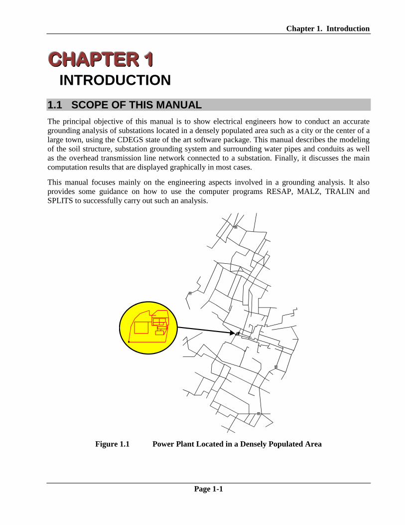
The principal objective of this manual is to show electrical engineers how to conduct an accurate

grounding analysis of substations located in a densely populated area such as a city or the center of a

large town, using the CDEGS state of the art software package. This manual describes the modeling

of the soil structure, substation grounding system and surrounding water pipes and conduits as well

as the overhead transmission line network connected to a substation. Finally, it discusses the main

computation results that are displayed graphically in most cases.

This manual focuses mainly on the engineering aspects involved in a grounding analysis. It also

provides some guidance on how to use the computer programs RESAP, MALZ, TRALIN and

SPLITS to successfully carry out such an analysis.

Figure 1.1 Power Plant Located in a Densely Populated Area


Page 1-2

1.2 EXAMPLE USED AS A REFERENCE

This manual is based upon a two-phase study, performed by SES, of a Power Plant grounding

system. The study, initially a preliminary or exploratory study, has matured into a sophisticated in-

depth study of the conductive performance of the entire grounding network skeleton extending

between the Power Plant and its neighboring substations, which are interconnected via overhead

transmission lines.

1.3 COMPUTER SOFTWARE USED

The study presented in this manual is based on computer simulations performed with the programs

RESAP, MALZ, TRALIN, and SPLITS of the CDEGS Software package. In order to enable the

reader to assimilate and put to practical use the material as quickly as possible, a few computer input

files used in the example analyses are provided with this manual (see Section 1.8 below). The

Windows Toolbox Input Mode and /or SICL (SES Input Command Language) input format have

been selected for these input files to make them easier to understand. Output from the computer

programs, mainly in the form of plots generated by the Windows Output Toolbox (SWOMS) and the

SES Interactive Report & Plot Software processors (such as GraRep), has also been included

wherever possible.

1.4 ORGANIZATION OF THIS MANUAL

This manual is, to a large extent, a detailed example of how to carry out a conductive/grounding

analysis with the aid of the CDEGS computer software. Each chapter describes one step in the

analysis process by showing what was done in the study.

Chapter 2 outlines the methodology followed by the study. The soil resistivity measurement and

interpretation processes using RESAP are discussed in Chapter 3. Chapter 4 describes how to model

metallic conductor networks including substations, water pipes and other conduits. It also illustrates

how to build an input file and how to compute the GPR of a conductor network using the MALZ

program. Chapter 5 describes how to model and compute line parameters using the TRALIN

program. Chapter 6 explains how to use the results obtained in Chapter 5 to build the transmission

line network required by the SPLITS program. SPLITS results are also discussed and displayed in

this chapter. Finally, Chapter 7 presents the overall grounding performance of the Power Plant based

on the computed results obtained from MALZ. It also discusses mitigation measures. Most results

are presented in graphical form.

1.5 SOFTWARE NOTE

This tutorial assumes that the reader is using the Windows version of CDEGS.

1.6 FILE NAMING CONVENTIONS

It is important to know which input and output files are created by the CDEGS software. All CDEGS

input and output files have the following naming convention:


Page 1-3

XY_JobID.Fnn

where XY is a two-letter abbreviation corresponding to the name of the program which created the

file or which will read the file as input. The JobID consists of string of characters and numbers that

is used to label all the files produced during a given CDEGS run. This helps identify the

corresponding input, computation, results and plot files. The nn are two digits used in the extension

to indicate the type of file.

The abbreviations used for the various CDEGS modules are as follows:

Application Abbreviation Application Abbreviation

RESAP RS FCDIST FC

MALT MT HIFREQ HI

MALZ MZ FFTSES FT

TRALIN TR SICL* SC

SPLITS SP CSIRPS* CS

SESTLC TC SESEnviroPlus TR

SESShield LS SESShield-3D SD

GRSPLITS-3D SP ROWCAD RC

* The SICL module is used internally by the Input Toolbox data entry interface. The CSIRPS

module is used internally by the Output Toolbox and GRServer – graphics and report

generating interface.

The following four types of files are often used and discussed when a user requests technical support

for the software:

.F05 Command input file (for engineering applications programs). This is a text file that can

be opened by any text editor (WordPad or Notepad) and can be modified manually by

experienced users.

.F09 Computation results file (for engineering applications programs). This is a text file that

can be opened by any text editor (WordPad or Notepad).

.F21 Computation database file (for engineering applications programs). This is a binary file

that can only be loaded by the CDEGS software for reports and graphics display.

.F33 Computation database file (for engineering applications programs MALZ and HIFREQ

only). This is a binary file that stores the current distribution to recover.

For further details on CDEGS file naming conventions and JobID, please consult CDEGS Help

under Help | Contents | File Naming Conventions.


Page 1-4

1.7 WORKING DIRECTORY

A Working Directory is a directory where all input and output files are created. In this tutorial, we

recommend the following Working Directory:

C: (or D:)\CDEGS Howto\Urban\

You may prefer to use a different working directory. Either way, you should take note of the full

path of your working directory before running CDEGS, as you will need this information to follow

this tutorial.

1.8 INPUT AND OUTPUT FILES USED IN TUTORIAL

There are two ways to use this tutorial: by following the instructions to enter all input data manually

or by loading the input files provided with the tutorial and simply following along.


Page 1-5

All input files used in this tutorial are supplied on your DVD. These files are stored during the

software installation under documents\Howto\CDEGS\Urban (where documents is the SES software

documentation directory, e.g., C:\Users\Public\Documents\SES Software\version, and version is the

version number of your SES Software) Note that this folder is a distinct folder than the SES software

installation directory, e.g, C:\Program Files\SES Software\version (where version is, again, the

version number of your SES Software).

Copying Input Files to Working Directory

For those who prefer to load the input files into the software and simply follow the tutorial, you can

copy all of the files from the documents\Howto\CDEGS\Urban directory to your working directory.

After the tutorial has been completed, you may wish to explore the other How To…Engineering

Manuals which are available as PDF files on the SES Software DVD in the folder \PDF\Howto.

If the files required for this tutorial are missing or have been modified, you will need to manually

copy the originals from the SES Software DVD.Both original input and output files can be found in

the following directories on the SES Software DVD:

Input Files: Examples\Official\HowTo\CDEGS\Urban\inputs

Output Files: Examples\Official\HowTo\CDEGS\Urban\outputs

Note that the files found in both the ‘Inputs’ and the ‘Outputs’ directories should be copied directly

into the working directory, not into subdirectories of the working directory.

Chapter 2. General Outline of the Study

Page 2-1


GENERAL OUTLINE OF THE STUDY

2.1 OBJECTIVES

The principal objective of the study is to determine the voltages inside and outside the Power Plant

following a phase-to-ground fault at the Power Plant. These voltages can then be evaluated in terms

of safety to personnel and the general public and any detrimental effects they may have on

equipment. If these are found to be unacceptable, then various mitigation means can be studied and

implemented.

2.2 MOTIVATION

Before conducting any detailed study of an existing substation, it is always advisable to review

pertinent drawings and documentation, carry out site visits and engage in detailed discussions with

key personnel involved with the design and operation of the substation. Such activities help identify

the best course of action to be taken and the most appropriate methodology for the study.

These steps revealed that the performance of the Power Plant is very likely to be heavily influenced

by the numerous interconnections between the substation's buried metallic pipes and those existing

in its neighborhood, several blocks and even miles away within the city.

Generally, most buried pipes are bonded to the grounding system directly or via the neutral wires of

the distribution system. While the GPR and local touch voltage magnitudes are essentially dictated

by the amount of fault current dissipated locally and by earth structure characteristics, the

magnitudes of touch voltages and potential differences between different parts of metallic structures

and their attenuation along the extensive metallic network are largely a function of the cross section,

length and electrical characteristics of the conductor path taken by the current to return to the source.

In practice, all of these voltages may be excessive and result in unsafe situations or cause operational

disruption. When excessive voltages are the result of an excessive GPR, reducing the resistance of

the grounding system and increasing the number of meshes in the grounding system result in a

reduction of the electrical stresses. Problems associated with potential differences (such as touch

voltages) are reduced by bonding techniques based on topological considerations aimed at

establishing equipotential zones to prevent simultaneous access to metallic parts raised at

significantly different potentials.

All these considerations suggest that an accurate analysis of the Power Plant requires that the entire

metallic network be modeled. However a preliminary, exploratory conservative analysis based on

modeling the Power Plant grounding system alone may reveal that the substation grounding

performance is safe and operationally adequate.

The first step in a study such as this one is therefore to investigate the limiting case scenario where

the majority of the fault current is assumed to dissipate locally (i.e., in the Power Plant grounding


Page 2-2

system and local metallic pipes to which it is connected) in the earth. For this scenario, the nature of

the soil structure and characteristics of its various layers are key parameters in determining the

performance of the grounding system. If the exploratory study reveals that the computed values

exceed the safe limits, then a detailed study is needed to determine whether the excessive levels

result solely from the conservatism of the initial study or if mitigation measures are truly required.

Since the detailed study demonstrates all of the computer modeling required for this type of analysis,

the remainder of this manual discusses a detailed study of the Power Plant.

2.3 METHODOLOGY

To complete the study, the following steps were followed.

1. Soil Resistivity Analysis: Using the RESAP program, the equivalent soil structures, based

on the measured soil resistivity data, were determined. (Chapter 3)

2. Substation Grounding Network and Water Pipe Modeling: A conductor network model

was built, including the Power Plant grounding network, the associated fence and an

extensive water pipe network in the area occupied by the Power Plant, the Substation North,

Plant West, Substation East and Substation South. Furthermore, the Power Plant grounding

impedance was computed using the MALZ program. (Chapter 4)

3. Transmission Line Modeling: The transmission lines connecting the plant substations

mentioned in Step 2 were modeled, and the TRALIN program was used to compute the line

parameters such as self and mutual impedances of the transmission lines. (Chapter 5)

4. Fault Current Determination: Using the Power Plant ground impedance and the line

parameters obtained in Steps 2 and 3, a multi-terminal circuit model was built.

Subsequently, the SPLITS program was used to compute the fault current distribution for a

fault at the Power Plant. (Chapter 6)

5. Computation of Potentials, Touch and Step Voltages: The MALZ program was used to

compute the earth surface potentials, and the touch and step voltages, inside and outside the

Power Plant, using the conductor network built in Step 2, the fault current injected in the

Power Plant grounding network and at other substations as computed in Step 4. (Chapter 7)

In summary, the equivalent soil model is determined, the Power Plant grounding network is modeled

in conjunction with the surrounding water pipes and conduits, and the impedance of the grounding

network is calculated. Next, the transmission lines are modeled and, based on the fault currents

provided, the currents injected into the grounding network and the other substations are computed.

Finally, various electric quantities such as the GPRs of the grounding network, the earth surface

potentials, and the touch and step voltages, inside and outside the Power Plant are examined.

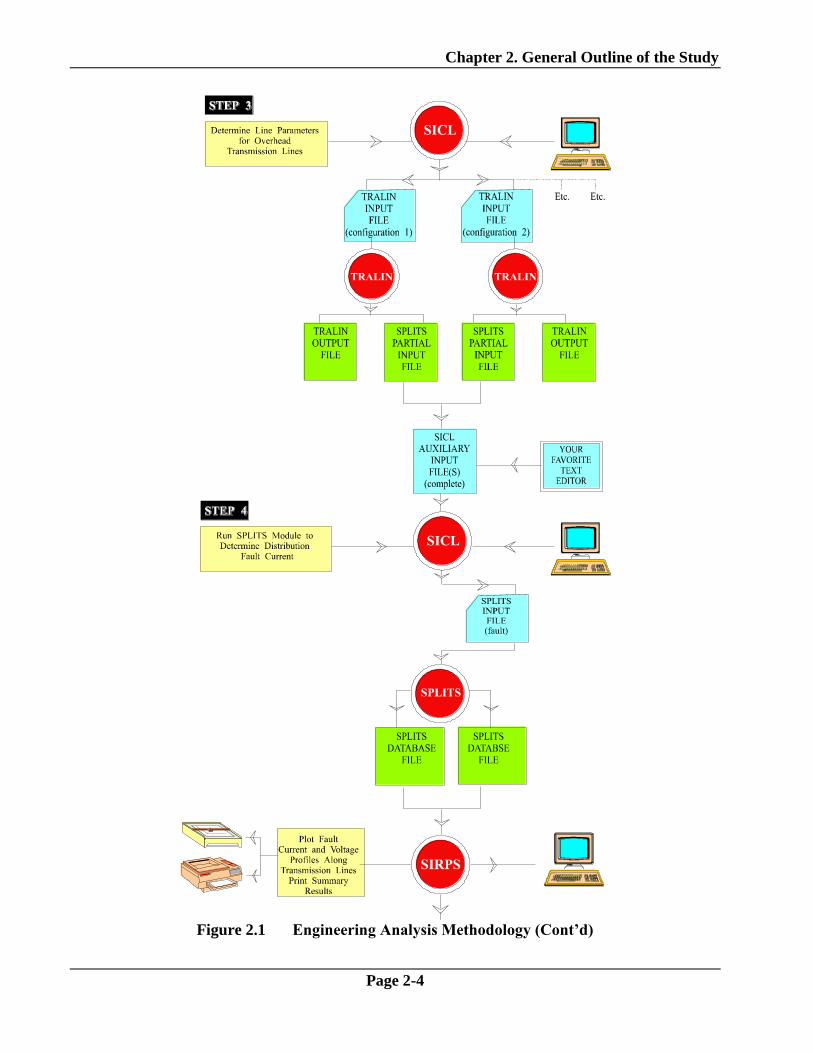
The methodology followed by this study is illustrated in Figure 2.1. Please note that the short-circuit

level selected in this study does not correspond to a real case and is used for illustration and

academic purposes only.


Page 2-3

Figure 2.1 Engineering Analysis Methodology


Page 2-4

Figure 2.1 Engineering Analysis Methodology (Cont’d)


Page 2-5

Figure 2.1 Engineering Analysis Methodology (Cont’d)

Chapter 3. Soil Resistivity Analysis

Page 3-1


SOIL RESISTIVITY ANALYSIS

This chapter presents the soil resistivity analysis. The program used to carry out the analysis is

RESAP.

The RESAP program determines the best combination of layer resistivities and thicknesses for a

multilayer earth model that minimizes the RMS error between the computed and measured apparent

soil resistivity curves.

An equivalent multilayer soil model is obtained using the RESAP program based on soil resistivity

measurements made using the Wenner 4-Point Method along a traverse. The program can obtain

excellent fits to the data without any user intervention.

3.1 MEASUREMENT RESULTS

Usually, when the electrode penetration into the earth is shallow, the relationship between measured

apparent resistances and resistivities can be approximated as follows:

2 aR (a in m)

or

1915. aR (a in feet)

where is the apparent soil resistivity in -m, a is the electrode spacing and R is the measured

apparent resistance in .

In order to accurately determine the grounding performance of a substation with a size comparable to

our site, it is necessary to carry out resistivity measurements along a traverse (preferably two

traverses orthogonal to each other) which extends at least twice the largest dimension of the

substation. In the case of the Power Plant, a traverse length of 1500 or more is required to establish

the soil structure with a reasonable degree of confidence for the computer analysis. Table 3–1 lists

the apparent resistances measured along a traverse and Figure 3.1 is a plot of these data values (dots)

which have been converted into apparent resistivities by RESAP (see next).


Page 3-2

Separation Depth of Depth of Apparent

Between

Probes

Current

Probes

Potential

Probes

Resistance

(V/I)

(feet) (feet) (feet) (ohms)

0.5 0.08 0.08 46.50

1.0 0.33 0.17 19.03

1.5 0.33 0.17 16.06

2.5 0.33 0.17 12.86

4.0 1.0 0.50 11.18

7.0 1.0 0.50 8.55

10.0 1.0 0.50 7.10

15.0 1.5 1.0 5.44

25.0 1.5 1.0 4.05

40.0 1.5 1.0 2.01

70.0 1.5 1.0 0.53

100.0 1.5 1.0 0.17

150.0 1.5 1.0 0.06

250.0 1.5 1.0 0.04

400.0 1.5 1.0 0.03

500.0 1.5 1.0 0.03

Table 3–1 Measured Apparent Resistances of Power Plant Using the Wenner Method

3.2 A FOUR-LAYER SOIL MODEL

A RESAP input file RS_URBRAuto.F05 corresponding to the soil resistance measurement values

listed in Table 3–1 is prepared by using the Windows Input Toolbox. Chapter 3 of the How

To…Engineering Guide titled “A Simple Substation Grounding Analysis” provides detailed

descriptions on how to prepare a RESAP input file using the Windows Input Toolbox and run

RESAP engineering program to obtain an equivalent soil model. Figure 3.1 shows the computed

apparent resistivity curve (dashed line) together with the measured data points (dots). A four-layer

soil model shown in Table 3–2 is obtained.


Page 3-3

10-1 100 101 102 103

Inter-Electrode Spacing (feet)

100

101

102

103

Ap

pa

ren

tR

es

isti

vit

y(O

hm

-me

ters

)

LEGEND

Measured Data

Computed Results Curve

Soil Model

Measurement Method..: Wenner

RMS error...........: 6.27%

Layer Resistivity Thickness

Number (Ohm-m) (Feet )

====== ============== ==============

Air Infinite Infinite

2 41.51522 2.104832

3 282.4221 25.65171

4 1.538804 18.02421

5 44.84925 Infinite

British/Logarithmic X and Y

RESAP <URBRAUTO >

Figure 3.1 Soil Resistivity Data verses Computed Apparent Resistivity

Figure 3.2 Equivalent Four-Layer Soil Model

In theory, the apparent soil resistivity curve should become horizontal at very large and very small

electrode spacings. In practice, however, the portions of the curve just beyond the smallest and the

largest measured electrode spacings are often sloped due to the limited range of measurements. In

this case, engineering judgment must be used to determine the orientations of the curve beyond the

smallest and the largest spacings and ensure that the computed soil resistivity curve will fit the

measured data points within the range of measured spacings.

For example, in Figure 3.1, the measured resistivity at 0.5 spacing is slightly higher than the

measured resistivity at 1 spacing. Being conservative in the interpretation, the measurement at 1


Page 3-4

spacing can be ignored and an assumption made that the measured curve is flat between spacings 0.5

and 1.5. For larger electrode spacings (150), the curve rises rapidly and, at the end of this chapter

(Section 3.4), it will be shown that this sharp rise could be due to the inductive coupling between the

current electrode leads and the voltage electrode leads. It is the responsibility of the user to follow

the procedure described in Section 3.4 to ensure the validity of the measured data. In this chapter,

however, they will be treated as legitimate measurement points in the interpretation process, just to

demonstrate how to handle a valid rise in the measured resistivity curve, should one occur.

Figure 3.1 illustrates that the fit between the computed and the measured soil resisitivity values is

good. Physically, as the probe spacing increases, so does the volume of earth encompassed by the

test current in its passage from one current electrode to the other, and so does the depth of earth

involved in the measurement. The measurements at short electrode spacings correspond to the top

soil layer resistivities and the measurements at large electrode spacings correspond to the deeper soil

layer resistivities.

The shape of the measured data points and computed resistivity curve in Figure 3.1 indicates the

following soil layering:

1. A medium resistivity top layer, corresponding to measurements at electrode spacings ( 2.5).

2. Beneath the top layer, a second layer with a much higher resistivity, as suggested by the

sharp rise in the measured soil resistivities at spacings between 2.5 and 25.

3. A third layer with a resistivity lower than the second layer, because the measured soil

resistivity values at electrode spacings between 100-200 are lower than those of the second

layer.

4. A bottom layer corresponding to the part of the curve that eventually flattens out at very large

spacings (beyond 500'). Even though the measured curve does not extend far enough to show

this section, it should still be accounted for in the analysis.

Note that the number of hills and valleys in the soil resistivity curve (both computed and measured)

does not necessarily correspond to the number of soil layers in the model. It may happen that several

soil layers are responsible for one single peak (or valley) in the soil resistivity curve. If the estimated

soil model has fewer layers than the true soil structure, the fit may never be satisfactory no matter

what resistivities and thicknesses are specified for the estimated model. Therefore, before starting

any iterative improvement of the curve fitting, the user has to analyze the shape of the measured

resistivity curve as described earlier and determine the minimum number of layers in the soil model

to be specified. If no fit can be found after several attempts with various combinations of soil

parameters, a soil model with a greater number of layers than the minimum should be considered.

Note also that the fit obtained using the iterative approach is not necessarily the best fit. Some

computational instability could occur when the measured data contains noise or does not lie on a

smooth curve. In such cases, the user has to remove the noisy points manually from the input file in

order to obtain a good fit. Please consult the on-line help (by pressing F1 key in the Soil-Type screen

in the RESAP Input Toolbox) for further details.


Page 3-5

3.3 OTHER RESAP RUNS

Several other RESAP runs were made, corresponding to resistivity measurements along different

traverses. In the end, an average three-layer soil model representative of the entire range of

measurements was selected. This soil model is used in the remainder of this manual.

Layer Resistivity (-m) Thickness (feet)

Top 44.5 3.43

Central 494 15.4

Bottom 17.4

Table 3–2 Three-Layer Soil Model Used for Grounding Analysis

3.4 POSSIBLE SOURCES OF NOISE IN THE MEASUREMENTS

Besides the procedure for soil resistivity curve fitting, it is important to realize that accurate

measurements constitute the basis for any sound soil resistivity interpretation. It is very important for

a RESAP user to be aware of the possible sources of errors and to take the necessary precautions to

avoid these errors or discard some measurements with non-correctable errors. The main sources of

errors include the following:

Instrument Error

Instrument error can be due to weak batteries or lack of recent calibration. Having additional

instruments on hand to verify the readings of the primary instruments allows this type of error to be

identified.

Electromagnetic Noise Due to Nearby Sources

The most common source of noise originates from electric power systems. Noise at a frequency of

60 Hz and its harmonics can be induced in the potential probe leads by power lines which are

parallel to the leads or at a shallow angle to them. This noise is generated by the electromagnetic

field surrounding the power lines. Ground return currents flowing in the earth from one part of the

power system to another constitute another source of noise. The magnitude of the noise is typically

directly proportional to the probe spacing, whereas the strength of the signal to be measured is

inversely proportional to the probe spacing. Thus, for short probe spacings, noise may be negligible

compared to the strength of the signal, but will eventually become larger than the signal if the probe

spacing increases too much. The magnitude of the noise voltage can be measured between the

potential probes, with the signal generator off. If it is on the same order as the signal, then special

measures must be adopted to filter out the noise from the measurements.

Coupling Between Leads


Page 3-6

As has been mentioned at the beginning of this chapter, the sharp rise in the measured resistivity

curve at large spacings in Figure 3.1 could be due to inductive coupling between the current probe

leads and the potential probe leads. For soil resistivities on the order of 100 -m or more and probe

spacings on the order of 100 feet or less, this inductive coupling is not a significant problem.

However, for larger probe spacings and lower soil resistivities, significant noise problems can be

encountered due to this coupling. The strength of this noise signal is roughly proportional to the

signal frequency. If measurements are made at one frequency and then repeated at a significantly

higher frequency, an inductive coupling problem will be revealed by a considerable difference

between the apparent resistivities measured at the two frequencies. When significant coupling is

experienced, the measured data should be either corrected by subtracting the inductive coupling

component or discarded if not recoverable. If possible, the user can also avoid or mitigate this

problem by working at DC or very low frequencies.

Nearby Buried Metallic Structures

If the resistivity measurements are carried out too close to bare metallic structures, such as water

pipes or grounding systems, then the measured apparent resistivities will be lower than the true

values representative of the actual soil structure. To avoid this problem, the solution is obvious: stay

as far away from bare metallic structures as possible. It is not always easy, however, to do so.

Furthermore, when soil resistivity measurements are being carried out for the analysis of an existing

grounding system, one wants to remain as close as possible to the grounding system, without being

so close that false readings are obtained due to the influence of the grounding system.

Chapter 4. Conductor Network Modeling

Page 4-1


CONDUCTOR NETWORK MODELING

The electric Power Plant and substations are centrally located in the city, near a large river, which

crosses the city from west to east. The Power Plant is interconnected via 69 kV transmission lines to

the Substation East, and electric substations North, West and South. It is surrounded by a metallic

fence that can be contacted by the public and city employees. Several major water lines and two 12"

gas pipelines are present in the Power Plant area and extend to other locations, including a water

treatment plant located about one hundred feet away on the east side of substation. A railway track

and various business offices are located on the north side of the Power Plant. The Power Plant

dimensions are about 800 ft 700 ft.

Because the water and gas pipes are bonded to the grounding system directly and indirectly via

neutral wires of the distribution feeders of the city, the overall ground conductor network extends for

miles around the Power Plant. Therefore, this extensive network must be modeled if accurate results

are required.

Attempts to model in detail every major component of this ground network quickly lead to computer

time and memory limitations. Fortunately, however, it is conservative and reasonably accurate to

model only a skeleton of this network, consisting of the major pipes and metal structures connected

to the Power Plant.

Our main objective in this chapter is to build the ground conductor network and to compute the

Power Plant ground impedance for two cases:

The Power Plant grounding system alone (for reference only).

The entire ground network buried in the extensive area occupied by the Power Plant,

Substation North, Plant West, Substation South and Substation East.

4.1 THE POWER PLANT GROUNDING SYSTEM

The Power Plant grounding network consists of the following major components:

The grounding system of the substation.

The buried portion of the substation metallic fence and ground loops.

The buried portion of the Power Plant property metallic fence and ground loops.

The rebars of the concrete floor of the Power Plant building. This part of the Power Plant is

simulated by a peripheral ground conductor loop. Additional wire meshes were added later

to enhance this simulation.

These components were identified from the Power Plant grounding layout drawings provided by the

city. The lengths of the grounding conductors were measured and the coordinates were obtained


Page 4-2

from the drawings. There are 18 vertical rods in the grounding system. They were not modeled

because they have only a small influence on the performance of this large grounding system.

The detailed Power Plant grounding system including fence loops is shown in Figure 4.1. Rebars in

reinforced concrete can be treated as a very dense ground grid because concrete will exhibit a

resistivity comparable to the local soil in which it is embedded. Again, it would be impractical to

model all the rebars. Hence, a less dense conductor mesh is shown in Figure 4.1. Figure 4.2 shows a

reduced version of the grounding system that was used together with the water pipe network to build

a MALZ input file. Use of the reduced grounding system reduces computation time. For touch

voltages, the reduced grounding system gives higher values than the detailed grounding system and

thus makes the study more conservative. The reduced grounding system will have a slightly higher

ground impedance than that of the detailed grounding system. The difference will be small because

the ground impedance is dependent mainly on the area covered by the grounding grid and is

relatively insensitive to the conductor density of the grid.

Figure 4.1 Detailed Grounding System of the Power Plant


Page 4-3

Figure 4.2 Reduced Grounding System of the Power Plant

4.2 THE PIPE NETWORK OUTSIDE THE POWER PLANT

The underground water pipes outside the Power Plant are identified on the layout drawings provided

by the city. They were sketched on a copy of the city-map from which the coordinates of the pipes

were then obtained. The pipe networks together with the reduced grounding system are shown in

Figure 4.3. It can be seen that the modeled pipe network covers an area of 10 miles 6 miles. There

are eleven different sizes of pipes. The radii of the pipes range from 6" to 33". It should be noted

that in the modeling of the pipe network, pipes with radii smaller than 6" were ignored because some

of them may be PVC pipes. Ignoring these smaller pipes makes the study more conservative. A


Page 4-4

rebar reinforced concrete pipe can be treated as a metallic pipe because its grounding effect is similar

to that of a metallic pipe.

Figure 4.3 Complete Conductor Network: Power Plant Grounding System with Pipe

Network

4.3 THE MALZ INPUT FILES

Once the coordinates of the complete conductor network are obtained, the construction of a MALZ

input file MZ_REDU.F05 is a rather simple matter. The conductors of the grounding system are

modeled as copper conductors. The water pipes are made of steel with a resistivity equal to 17 times

that of copper and a permeability of 300 times that of air. In addition, it is assumed that no coating is

present for any of the water pipes. It should be mentioned that in the actual MALZ run, pipes with


Page 4-5

radii larger than 15" are changed to smaller pipes with radii of 12". This is because the larger pipes

cut the soil layer interface and result in computational problems. For a uniform soil, these problems

do not exist. Two MALZ runs using a uniform soil with changed and unchanged pipe radii revealed

that the results are very close.

The soil model used in the MALZ run is the three-layer soil model in Table 3–2.

The MALZ run corresponding to the complete network shown in Figure 4.3 gives a GPR of –1245.7

+ j 1819.6 volts at the injection point of the grounding system. This value is obtained from the

MALZ output file MZ_REDU.F09 (Searching for string “GPR” will bring you to the appropriate

location quickly). The injection current is 4875 + j 24510 A, which is an approximate estimate of the

total available fault current. Therefore, the impedance of the grounding system at the current

injection point is:

(-1245.7 + j 1819.6)/(4875.0 + j 24510.0) = 0.062 + j 0.063

The injection point was assumed to be located at the lower left corner of the Power Plant as shown in

Figure 4.3.

It should be pointed out that in computing the impedance of the grounding system, one can use any

nominal injection current such as 1000 A. Here we used the approximate total available fault

current.

In order to compare the ground impedances of the detailed and reduced grounding systems, two

more MALZ runs using a uniform soil of 100 -m were carried out.

The MALZ run corresponding to the detailed grounding system leads to an impedance of 0.295 + j

0.086 ohms.

The MALZ run corresponding to the reduced grounding system results in an impedance of 0.309 + j

0.084 ohms.

It can be seen from the preceding results that the difference between the two ground impedances is

less than 5%. When the entire pipe network is considered, this difference will be even smaller.

The ground impedance of the complete network is used in the SPLITS runs as described in Section

6.3

Chapter 5. Computation of Transmission Line Parameters

Page 5-1


COMPUTATION OF TRANSMISSION LINE

PARAMETERS

The touch and step voltages associated with the grounding network are directly proportional to the

portion of fault current discharged directly into the soil. It is therefore critical to determine how

much of the fault current returns via the skywires of the transmission lines feeding the Power Plant.

In order to be able to determine the actual fault current split, the overhead transmission conductor

network must be modeled as described in Chapter 6. Before this however, it is necessary to calculate

accurately transmission line parameters such as self and mutual impedances and capacitances

between transmission line conductors at various transmission line span locations with varying

configurations.

This is done in this chapter, which shows how to compute the transmission line parameters using

program TRALIN. The resulting parameters will be used to build the input file for program SPLITS

to compute the fault current distribution.

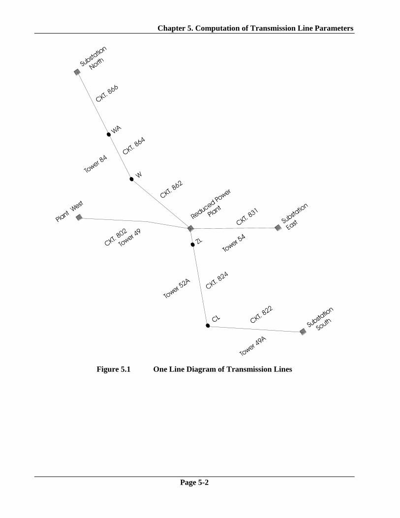
5.1 TRALIN INPUT FILE

A simple single line diagram of the transmission lines running between the Power Plant, Substation

North, Plant West, Substation South and Substation East is shown in Figure 5.1. Typical

transmission line cross sections as provided by the city have been chosen for the transmission lines

between the Power Plant and the other substations and plants. Tower 84 is a representative structure

between the Power Plant and Substation North; Tower 49 is a typical structure between the Power

Plant and Plant West; Tower 54 represents the structures between the Power Plant and Substation

East; and Towers 52A and 49A depict typical structures between the Power Plant and Substation

South (See Figure 5.1 for an indication of where these structures are located). The cross sections

corresponding to these representative towers are shown in Figure 5.2 to Figure 5.6. It should be

noted that the heights of the conductors indicated in the figures are average values accounting for a

sag of 18.

Five TRALIN input files (TR_TWR84.F05, TR_TWR49.F05, TR_TWR54.F05, TR_TW52a.F05

and TR_TW49a.F05) were built corresponding to the five representative towers. The phase

conductors are 795 kcmil ACSR 26/7 Drake and the skywires are 3/8" EHS. The coordinates of the

conductors are specified using the GROUP command in the TRALIN input files. The characteristics

of the conductors are specified by the STRANDS command. See the TRALIN manual for details of

the commands used in the input files.


Page 5-2

Figure 5.1 One Line Diagram of Transmission Lines


Page 5-3

Figure 5.2 Tower 84: Representative Structures Between Power Plant and Substation

North.

Figure 5.3 Tower 49: Representative Structures Between Power Plant and Plant West.


Page 5-4

Figure 5.4 Tower 54: Representative Structures Between Power Plant and Substation

East.

Figure 5.5 Tower 52A: Representative Structures Between Power Plant and Substation

South.


Page 5-5

Figure 5.6 Tower 49A: Representative Structures Between Power Plant and Substation

South.

5.2 TRALIN OUTPUT

By running TRALIN, several output files were obtained. One of the output files is TR_JOBID.F27

(where "JobID" is the job identification used to label the runs).

This file contains line parameters in the form of SPLITS input file commands around which a

complete SPLITS input file can be prepared. Five TRALIN output files are obtained corresponding

to the five different cross sections. It should be noted that in these files the series and mutual

impedances are in /mile and the shunt impedances are in -miles. They are converted into "ohms

per span" in the SPLITS input file using the "span-scaling" option as explained in the next chapter.

Chapter 6. Computation of Fault Current Distribution

Page 6-1


COMPUTATION OF FAULT CURRENT

DISTRIBUTION

The TRALIN runs discussed in Chapter 5 produced the line parameters needed to construct the

overhead transmission line network specification in the SPLITS input file. Figure 6.1 shows the

circuit model that was used to compute the fault current distribution for a ground fault at the Power

Plant. The average span length (distance between two adjacent towers) is 300 feet. Based on the

provided transmission line lengths between the Power Plant and other substations, there are 29 spans

from the Power Plant to Substation North, 52 spans from the Power Plant to Plant West, 43 spans

from the Power Plant to Substation East, and 64 spans from Power Plant to Substation South. For

simplicity, only the faulted phase conductor was modeled with a connection to its source. It would

have been a simple matter to include the other phases. This however would have been an

unnecessary sophistication in this context.

Substation

East

(EARTH)

Plant WestSubstation

North

Reduced Power

Plant

(Central Substation)

Substation

South

Phase A Phase B

Phase C

0.00.0

15 (Tower Impedance)

0.1

0.10.1

0.10.062 + j 0.063

Skywire

Equivalent Source

(Thevenin)

Impedance

Figure 6.1 Transmission Line Circuit Model


Page 6-2

6.1 SPLITS INPUT FILE

In the input file for the initial SPLITS run (SP_SGL1.F05), whose run identification is SGL1, the

impedance values corresponding to one mile are transformed into values corresponding to a 300 feet

span length by the SPAN-SCALING command and the span-scaling factor 0.05682

(300/5280 = 0.05682) at the end of the SECTION command. The central site is chosen to be the

Power Plant and there are four terminals specified in the input file, namely Substation North, Plant

West, Substation East and Substation South. Since a single phase fault is simulated, only one phase

conductor and the neutral wire are needed. However, the other two phase conductors in the input file

were not removed. Instead, zero voltages and infinite source impedances were specified for these

two phase conductors. The effect of this is equivalent to removing them. The command line

"GRID, OBSERVATION, 0.000001, 0.000001, 0.0" specifies the central site ground impedance as

0.000001+j0.00001 . This is because the fault current data provided by the city electrical

department is computed assuming that the Power Plant ground impedance is zero. Phase 4 represents

the skywire which has a typical shunt impedance of 15 . The value of 15 is the assumed ground

resistance of each of the towers modeled. It is a reasonable estimate based on the type of soil

structure found around the Power Plant. When the tower ground resistance is increased to 50 , the

fault current results decrease by about 4 percent.

Note that the source impedance of each terminal has been set to zero, meaning that the terminal is a

very strong (infinite) source of power.

6.2 SOURCE IMPEDANCE CALCULATION

In the first SPLITS run, SGL1, the phase conductor fault currents from each substation terminal are

as follows:

Substation North 6058.7 -79.96° A

Plant West 9985.3 -77.32° A

Substation East 14076.0 -77.73° A

Substation South 5196.4 -77.89° A

The fault currents provided by the city electrical department are:


Plant West 2299.9 -84.0° A



From the two sets of fault currents and source voltages, the correct equivalent terminal source

impedances can now be determined in order that the computed fault currents in a subsequent SPLITS

run match those provided by the city. Note that since the angles of the provided currents are a few

degrees smaller than those of the SPLITS currents, -5° is added to the source voltage angle and to the

angles of the SPLITS currents when computing the source impedances. This source voltage angle of

-5° will also be used in the subsequent SPLITS runs and the resulting SPLITS currents are expected


Page 6-3

to be close to the provided currents, both in magnitude and angle. Since in SPLITS run SGL1 the

source impedances are almost zero (0.00001 + j0.0 ), the equivalent line impedance as seen from

the Power Plant will be the ratio of the source voltage to the fault current. Take the Substation

North, for example:

39.8 -5.0° kV/6058.7 -84.96° A = 6.569179.96°

is the equivalent line impedance. It should be noted that 39.8 kV is the phase-to-ground voltage of

the 69 kV transmission line. The total circuit impedance (source impedance + equivalent line

impedance) based on the fault current value provided by the city is:

39.8 -5.0° kV / 4330.5 -84.0° A = 9.1906 78°

Hence the source impedance is:

9.1906 78° - 6.5691 79.956° = 0.77 + j2.52

The source impedances for all terminals are obtained in a similar manner. The final results are as

follows:

Substation North 0.77 + j2.52

Plant West 3.40 + j12.88

Substation East 0.11 + j0.87

Substation South 1.05 + j3.32

These source impedances are used in SPLITS run SGL2 whose input file is SP_SGL2.F05. The fault

currents obtained from SPLITS run SGL2 are:


Plant West 2300.0 -80.698° A



At this point, the currents from the SPLITS run SGL2 are very close to the fault currents provided by

the city electrical department.

Please note that the two SPLITS runs illustrated above can be reduced into a single SPLITS run by

using VIEnergizations at each terminal (a new feature in SPLITS). By specifying the source voltages

(V) and the fault currents (I) from the city electrical department at the same time, SPLITS program

will automatically determine appropriate source impedances at each terminal.

6.3 FINAL SPLITS RUN

The previous chapter describes how the correct source impedances were obtained, as indicated by

the close match between the computed fault currents and the corresponding currents provided by the


Page 6-4

city. The computed ground impedance of the central site (the Power Plant) can now be used to

simulate the real situation. The ground impedance is 0.062 + j0.063 and was computed as

described in Section 4.3.

From the final SPLITS run SGL3, the total fault current injected into the Power Plant grounding

system was obtained, as well as the currents discharged into the grounding system of each terminal

and each transmission line tower. The ground currents at each substation or plant are listed below:

The Power Plant: 17550 -89.86° A

Substation North: 3880.7 94.85° A

Plant West: 2051.2 96.30° A

Substation East: 9580.4 92.92° A

Substation South: 3190.6 95.89° A

The angle of the Power Plant current has approximately 180° difference with those of the other

substation currents. This fact indicates that the Power Plant current is out of phase with the

substation currents, as expected.

These currents will be used in Chapter 7 to determine the performance of the grounding system. The

terminal ground impedances (shown as EARTH in Figure 6.1) were assumed to be 0.1 , which is a

typical low value (conservative assumption). In fact, when 0.000001 is used instead of 0.1 , the

currents in the terminal grounds only change by about 4% and the current at the central site remains

almost identical. The substations along the transmission lines are not modeled. Since the ground

impedances of these intermediate substations are usually lower than the tower impedances, removal

of these substations will make the current in the central site higher because less current will flow into

the tower structure replacements of the substations through the skywire.

Chapter 7. Performance Analysis of the Grounding System

Page 7-1


PERFORMANCE ANALYSIS OF THE

GROUNDING SYSTEM

The computer model of the conductor network that consists of the grounding system and the

surrounding water pipes has been built. As well, the currents injected into the grounding system and

other substations in the case of a fault occurring at the Power Plant have now been computed. In this

chapter, the electric quantities that define the performance of the grounding network are now

examined. These electric quantities include the GPR of the grounding system, earth surface

potentials and touch and step voltages. The engineering computer program required for this analysis

is MALZ, which has the capability to handle large grounding networks including solid or hollow

conductors and bare or coated pipes in complex soil structures. The post-processing program SIRPS

is also used to obtain insightful plots of the computation results.

7.1 THE EQUIVALENT SOIL MODEL

In Chapter 4, the impedance of the grounding system was computed using a 3-layer soil model. By

changing the 3-layer soil model to a 100 -m uniform soil, a larger value of the impedance is

obtained. Since, for a uniform soil, the grounding system impedance is almost proportional to the

soil resistivity, it is easy to determine that a 76 -m uniform soil provides approximately the same

impedance as for the 3-layer soil case. A 76 -m uniform soil will be used in this study because this

will reduce the MALZ run time considerably. The whole grounding system together with the water

pipes covers such an extensive area that it would take many hours to complete some MALZ runs in

multi-layered soils.

7.2 MALZ INPUT FILE

A MALZ input file (MZ_RETU7.F05) with five energization busses (points) where the currents are

injected is used. These currents correspond to the fault current values discharged (or collected) by

the substation and plant grounding systems as computed in the previous chapter (Section 6.3). Figure

7.1 shows the complete conductor network with the injection currents.

7.3 COMPUTED RESULTS

Figure 7.2 shows a perspective view of the earth surface potentials in the vicinity of the Power Plant

(the area in Figure 4.2). Figure 7.3 shows numerous two dimensional plots of the reach touch

voltages which are defined as the difference between earth surface potentials and the GPR of a

conductor 5 feet away from the earth surface observation point. This is a conservative value

compared with the usual criteria of a 3 feet distance between the conductor and the earth surface

point. The large number of plots shown in this figure correspond to various profiles taken inside and


Page 7-2

nearby outside the Power Plant. Although one has difficulty seeing individual profiles, this figure

has the advantage of establishing the envelope of the maximum reach touch voltages observed in the

area covered by the profiles. Figure 7.4 shows the same reach touch voltages using a two-

dimensional spot map of the reach touch voltage magnitudes in the area covered by the profiles. It

can be seen that the high touch voltages occur around the left side and bottom of the fence. The

highest reach touch voltage is about 370 volts, and occurs outside the fence. Figure 7.5 shows the

maximum step voltages in the area covered by the profiles. It can be seen that the step voltages are

much smaller than the reach touch voltages.

Figure 7.1 Locations of Injection Currents


Page 7-3

Distance (feet)

Distance from Origin of Profile (Ft)

Po

ten

tia

lP

rofi

leM

ag

nit

ud

e(V

olt

s)

Scalar Potentials/Scalar Potentials [ID:RETU07 @ f=60.0000 Hz ]

0 200 400 600 8000

134

269

403

538

672

500

1000

1500

2000

Figure 7.2 Earth Surface Potentials in the Power Plant Area

0 200 400 600 800


0

100

200

300

400

R-T

ou

ch

Vo

lta

ge

Ma

gn

.(V

olt

s)

[Wo

rs]

Scalar Potentials/Reach Touch Voltages/Worst Spherical

V = 176 voltstouch_threshold

Figure 7.3 Reach Touch Voltage Profiles in the Vicinity of the Power Plant Area. Use

“Worst Spherical” and 5 ft “Search Radius for Reference GPR”.


Page 7-4

-200 300 800

X AXIS (FEET)

-200

300

800

YA

XIS

(FE

ET

)

R-Touch Voltage Magn. (Volts) [Wors]

Scalar Potentials/Reach Touch Voltages/Worst Spherical [ID:RETU07 @ f=60.0000 Hz ]

LEGEND

Maximum Value : 367.025

Minimum Value : 0.00

367.03

330.32

293.62

256.92

220.22

183.51

146.81

110.11

73.41

36.70

Figure 7.4 Two Dimensional Spot Depiction of Reach Touch Voltage Magnitudes in the

Vicinity of the Power Plant Area

0 200 400 600 800


0

50

100

150

Ste

pV

olt

ag

e-W

ors

tM

ag

nit

ud

e(V

olt

s)

Scalar Potentials/Step Voltages (Spherical)/Worst Spherical

Figure 7.5 Step Voltage Profiles in the Vicinity of the Power Plant Area


Page 7-5

7.4 SAFETY ASSESSMENT

For a fault clearing time of "t" seconds and a body resistance of 1 k the safe touch and step

voltages are given by the following expressions:

Vtouch_threshold = 116 + 0.174C

t s s

Vstep_threshold = 116 + 0.696C

t s s

where s represents the resistivity of the earth surface layer of soil and Cs is a correction factor

which is 1 when no surface covering layers exist. At the Power Plant where no special surface

covering materials are used, s is about 50 -m. Therefore we get:

Vtouch_threshold = 176 volts and Vstep_threshold = 213 volts

Clearly then, there are locations inside and outside the Power Plant where safety may be

compromised during ground faults because of high touch voltages. Some form of mitigation is

therefore necessary.

7.5 MITIGATIVE MEASURES

One of the simplest mitigative measures consists of covering the soil surface of the Power Plant with

a thin layer of high resistivity material such as crushed rock. This layer, with a thickness of about 6",

should extend at least 3 feet outside the Power Plant property fence to ensure public safety. The

resistivity of such a layer should be at least equal to 1000 -m (when wet) in order to render touch

voltages of 400 volts acceptable. This solution, however, is not practical in a Power Plant where its

presence may be intrusive and inconvenient for plant employees walking between various locations

in the Power Plant. Moreover, it may also introduce new maintenance problems and long term

integrity inspection problems.

Another more permanent and less apparent solution would be to reinforce the grounding system by

adding more ground conductors at all required locations. This solution is examined next.

Figure 7.6 shows an enhanced version of the grounding grid with additional conductors. First, it

should be noted that only a portion of the neighboring pipe network outside the Power Plant has been

modeled here. This conservative step was taken to avoid exceeding the capacity of the MALZ

program, while keeping computation time reasonable. A MALZ input file MZ_USMLR.F05

corresponding to the enhanced Power Plant grounding grid is prepared. Note also that the number of

conductors modeled has increased significantly because of the numerous new conductors introduced

inside the Power Plant. The total area covered by the ground network is 4000 ft 4000 ft. Note also

the absence of conductors at locations where trenching would be impractical or costly, i.e., below

concrete floors, at the old water treatment basins, etc. At such locations, however, the presence of


Page 7-6

metallic structures and slabs or rebars in concrete should hopefully provide safe equipotential

surfaces.

Figure 7.6 Complete Ground Network with Mitigation at the Power Plant

The computation results corresponding to this case are shown in Figure 7.7 to Figure 7.9. The

maximum GPR is 1483 volts and occurs at the fault current injection point. Figure 7.7 is a

perspective view of the earth surface potentials in the vicinity of the Power Plant. Figure 7.8 shows

the envelope of the maximum reach touch voltages in the same vicinity, while Figure 7.9 depicts the

same reach touch voltages using a spot map of the reach touch voltage magnitudes. Figure 7.8

clearly indicates that reach touch voltages are all below 160 volts except at two locations. One of

these locations corresponds to the area at the middle of the top of the fence. The other location

corresponds to the area at the bottom right corner of the fence. Both of the reach touch voltage

peaks occur outside the fence. If any metal pipes exist in these locations, which are connected to the

grounding system, the reach touch voltage peaks would be reduced.


Page 7-7

Distance (feet)


Po

ten

tia

lP

rofi

leM

ag

nit

ud

e(V

olt

s)

Scalar Potentials/Scalar Potentials [ID:USMLRF @ f=60.0000 Hz ]

0 200 400 600 8000

134

269

403

538

672

700

900

1100

1300

1500

Figure 7.7 Earth Surface Potentials in the Mitigated Power Plant Area

0 200 400 600 800


0

50

100

150

200

250

R-T

ou

ch

Vo

lta

ge

Ma

gn

.(V

olt

s)

[Wo

rs]

Scalar Potentials/Reach Touch Voltages/Worst Spherical

V touch_threshold = 176 volts

Figure 7.8 Reach Touch Voltage Profiles in the Vicinity of the Mitigated Power Plant

Area


Page 7-8

-200 300 800

X AXIS (FEET)

-200

300

800

YA

XIS

(FE

ET

)

R-Touch Voltage Magn. (Volts) [Wors]

Scalar Potentials/Reach Touch Voltages/Worst Spherical [ID:USMLRF @ f=60.0000 Hz ]

LEGEND

Maximum Value : 218.817

Minimum Value : 0.00

218.82

196.94

175.05

153.17

131.29

109.41

87.53

65.65

43.76

21.88

Figure 7.9 Two-Dimensional Spot Depiction of Reach Touch Voltage Magnitudes in the

Vicinity of the Mitigated the Power Plant Area

Chapter 8. Conclusions

Page 8-1


CONCLUSIONS

This concludes our concise instructions on how to conduct an accurate grounding analysis of

substations located in a densely populated area using the RESAP, MALZ, TRALIN and SPLITS

engineering modules.

Only a few of the many features of the software have been used in this tutorial. You should try the

many other options available to familiarize yourself with the CDEGS software package. Your SES

Software DVD also contains a wealth of information stored under the PDF directory. There you will

find the Getting Started with SES Software Packages manual (\PDF\getstart.pdf) which contains

useful information on the CDEGS environment. You will also find other How To…Engineering

Guides, Annual Users’ Group Meeting Proceedings and much more. All Help documents are also

available online.

Notes

NOTES